Embed Size (px)
Citation preview

–12
–2
017
-07-
03
–m
ain
–
Softwaretechnik / Software-Engineering
Lecture 12: Proto-OCL,
Modularisation & Design Patterns
2017-07-03
Prof. Dr. Andreas Podelski, Dr. Bernd Westphal
Albert-Ludwigs-Universität Freiburg, Germany
Topic Area Architecture & Design: Content–
12–
20
17-0
7-0
3–
Sb
lock
con
ten
t–
2/66
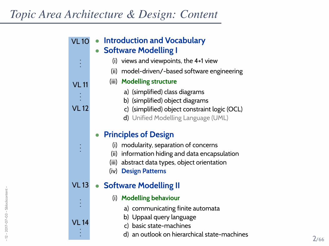
• Introduction and Vocabulary• Software Modelling I
(i) views and viewpoints, the 4+1 view
(ii) model-driven/-based software engineering
(iii) Modelling structure
a) (simplified) class diagrams
b) (simplified) object diagrams
c) (simplified) object constraint logic (OCL)
d) Unified Modelling Language (UML)
• Principles of Design(i) modularity, separation of concerns
(ii) information hiding and data encapsulation
(iii) abstract data types, object orientation
(iv) Design Patterns
• Software Modelling II
(i) Modelling behaviour
a) communicating finite automata
b) Uppaal query language
c) basic state-machines
d) an outlook on hierarchical state-machines
VL 10
...
VL 11...
VL 12
...
VL 13
...
VL 14...

Content–
12–
20
17-0
7-0
3–
Sco
nte
nt
–
3/66
• Proto-OCL
• syntax, semantics,
• Proto-OCL vs. OCL.
• Proto-OCL vs. Software
• An outlook on UML
• Principles of (Good) Design
• modularity, separation of concerns
• information hiding and data encapsulation
• abstract data types, object orientation
• . . .by example
• Architecture Patterns
• Layered Architectures, Pipe-Filter,Model-View-Controller.
• Design Patterns
• Strategy, Examples
• Libraries and Frameworks

–12
–2
017
-07-
03
–m
ain
–
4/66
Partial vs. Complete Object Diagrams–
11–
20
17-0
6-2
6–
So
d–
39/51
• By now we discussed “object diagram represents system state”:
{1C 7� {p 7� �, n 7� {5C}},5C 7� {p 7� �, n 7� �},1D 7� {p 7� {5C}, x 7� 23}}
�1C : C
p = �
5C : C
p = �
n = �
1D : D
x = 23
n p
What about the other way round. . . ?
• Object diagrams can be partial, e.g.
1C : C 5C : C 1D : D
x = 23
nor 1C : C 5C : C 1D : D
� we may omit information.
• Is the following object diagram partial or complete?
1C : C
p = �
5C : C
p = �
n = �
1D : D
x = 23
n p
• If an object diagram
• has values for all attributes of all objects in the diagram, and
• if we say that it is meant to be complete
then we can uniquely reconstruct a system state �.

–12
–2
017
-07-
03
–m
ain
–
5/66
Special Case: Anonymous Objects–
11–
20
17-0
6-2
6–
So
d–
40/51
If the object diagram
1C : C
p = �
: C
p = �
n = �
: D
x = 23
n p
is considered as complete, then it denotes the set of all system states
{1C 7� {p 7� �, n 7� {c}}}, c 7� {p 7� �, n 7� �}, d 7� {p 7� {c}, x 7� 23}}
where c � D(C), d � D(D), c 6= 1C .
Intuition: different boxes represent different objects.

Content–
12–
20
17-0
7-0
3–
Sco
nte
nt
–
6/66
• Proto-OCL
• syntax, semantics,
• Proto-OCL vs. OCL.
• Proto-OCL vs. Software
• An outlook on UML
• Principles of (Good) Design
• modularity, separation of concerns
• information hiding and data encapsulation
• abstract data types, object orientation
• . . .by example
• Architecture Patterns
• Layered Architectures, Pipe-Filter,Model-View-Controller.
• Design Patterns
• Strategy, Examples
• Libraries and Frameworks

Towards Object Constraint Logic (OCL)
— “Proto-OCL” —
–12
–2
017
-07-
03
–m
ain
–
7/66

Motivation–
12–
20
17-0
7-0
3–
So
cl–
8/66
C
D A
c 0,1
a
0,1
• How do I precisely, formally tell my developers that
All D-instances having a link to the same C objectshould have links to the same A.
• That is, the following system state is forbidden in the software:
: A : D : C : D : Aa c c a
Note: formally, it is a proper system state.
• Use (Proto-)OCL: “Dear developers, please only use system states which satisfy:”
∀ d1 ∈ allInstancesC • ∀ d2 ∈ allInstancesC • c(d1) = c(d2) =⇒ a(d1) = a(d2)

Constraints on System States–
12–
20
17-0
7-0
3–
So
cl–
9/66
Cx : Int
• Example: for all C-instances, x should never have the value 27.
∀ c ∈ allInstancesC • x(c) 6= 27
• Proto-OCL Syntax wrt. signature (T,C, V, atr , F,mth ), c is a logical variable, C ∈ C :
F ::= c : τC
| allInstancesC : 2τC
| v(F ) : τC → τ⊥, if v : τ ∈ atr(C)
| v(F ) : τC → τD, if v : D0,1 ∈ atr(C)
| v(F ) : τC → 2τD , if v : D∗ ∈ atr(C)
| f(F1, . . . , Fn) : τ1 × · · · × τn → τ, if f : τ1 × · · · × τn → τ
| ∀ c ∈ F1 • F2 : τC × 2τC ×B⊥ → B⊥
• The formula above in prefix normal form: ∀ c ∈ allInstancesC• 6= (x(c), 27)

Semantics–
12–
20
17-0
7-0
3–
So
cl–
10/66
• Proto-OCL Types:
• IJτCK = D(C) ∪̇ {⊥}, IJτ⊥K = D(τ) ∪̇ {⊥}, IJ2τC K = D(C∗) ∪̇ {⊥}
• IJB⊥K = {true, false} ∪̇ {⊥}, IJZ⊥K = Z ∪̇ {⊥}
• Functions:
• We assume fI given for each function symbol f (→ in a minute).
• Proto-OCL Semantics (interpretation function):
• IJcK(σ, β) = β(c) (assuming β is a type-consistent valuation of the logical variables),
• IJallInstancesCK(σ, β) = dom(σ) ∩ D(C),
• IJv(F )K(σ, β) =
{
σ (IJF K(σ, β)) (v) , if IJF K(σ, β) ∈ dom(σ)
⊥ , otherwise(if not v : C0,1)
• IJv(F )K(σ, β) =
{
σ(u′)(v) , if IJF K(σ, β) = {u′} ⊆ dom(σ)
⊥ , otherwise(if v : C0,1)
• IJf(F1, . . . , Fn)K(σ, β) = fI(IJF1K(σ, β), . . . , IJFnK(σ, β)),
• IJ∀ c ∈ F1 • F2K(σ, β) =
true , if IJF2K(σ, β[c := u]) = true for all u ∈ IJF1K(σ, β)
false , if IJF2K(σ, β[c := u]) = false for some u ∈ IJF1K(σ, β)
⊥ , otherwise

Semantics Cont’d–
12–
20
17-0
7-0
3–
So
cl–
11/66
• Proto-OCL is a three-valued logic: a formula evaluates to true, false, or ⊥.
• Example: ∧I(·, ·) : {true, false,⊥} × {true, false,⊥} → {true, false,⊥} is defined as follows:
x1 true true true false false false ⊥ ⊥ ⊥x2 true false ⊥ true false ⊥ true false ⊥∧I(x1, x2) true false ⊥ false false false ⊥ false ⊥
We assume common logical connectives ¬,∧,∨, . . . with canonical 3-valued interpretation.
• Example: +I(·, ·) : (Z ∪̇ {⊥})× (Z ∪̇ {⊥}) → Z ∪̇ {⊥}
+I(x1, x2) =
{
x1 + x2 , if x1 6= ⊥ and x2 6= ⊥
⊥ , otherwise
We assume common arithmetic operations −, /, ∗, . . .
and relation symbols >,<,≤, . . . with monotone 3-valued interpretation.
• And we assume the special unary function symbol isUndefined :
isUndefinedI(x) =
{
true , if x = ⊥,
false , otherwise
isUndefinedI
is definite: it never yields ⊥.

Example: Evaluate Formula for System State–
12–
20
17-0
7-0
3–
So
cl–
12/66
σ :1C : C
x = 13
Cx : Int
∀ c ∈ allInstancesC • x(c) 6= 27
• Recall prefix notation: ∀ c ∈ allInstancesC • 6=(x(c), 27)
Note: 6= is a binary function symbol, 27 is a 0-ary function symbol.
• Example:
IJ∀ c ∈ allInstancesC • 6=(x(c), 27)K(σ, ∅) = true, because. . .
IJ 6=(x(c), 27)K(σ, β), β := ∅[c := 1C ] = {c 7→ 1C}
= 6=I( IJx(c)K(σ, β), IJ27K(σ, β) )
= 6=I( σ( IJcK(σ, β) )(x), 27I )
= 6=I( σ( β(c) )(x), 27I )
= 6=I( σ( 1C )(x), 27I )
= 6=I( 13, 27 ) = true . . . and 1C is the only C-object in σ: IJallInstancesCK(σ, ∅) = {1C}.

More Interesting Example–
12–
20
17-0
7-0
3–
So
cl–
13/66
σ :1C : C
x = 13|
n Cx : Int n
0..1
∀ c : allInstancesC • x(n(c)) 6= 27
• Similar to the previous slide, we need the value of
IJx(n(c))K(σ, β), β = {c 7→ 1C}
• IJcK(σ, β) = β(c) = 1C
• IJn(c)K(σ, β) = ⊥ since σ( IJcK(σ, β) )(n) = ∅ 6= {u′} by rule
IJv(F )K(σ, β) =
{
u′ , if IJF K(σ, β) ∈ dom(σ) and σ(IJF K(σ, β))(v) = {u′}
⊥ , otherwise(if v : C0,1)
• IJx(n(c))K(σ, β) = ⊥ since IJn(c)K(σ, β) = ⊥ by rule
IJv(F )K(σ, β) =
{
σ (IJF K(σ, β)) (v) , if IJF K(σ, β) ∈ dom(σ)
⊥ , otherwise(if not v : C0,1)

More Interesting Example–
12–
20
17-0
7-0
3–
So
cl–
13/66
σ :1C : C
x = 13|
n Cx : Int n
0..1
∀ c : C • x(n(c)) 6= 27
• Similar to the previous slide, we need the value of
σ ( σ( IJcK(σ, β) )(n) ) (x)
• IJcK(σ, β) = β(c) = 1C
• σ( IJcK(σ, β) )(n) = σ( 1C )(n) = ∅
• σ ( σ( IJcK(σ, β) )(n) ) (x) = ⊥
by the following rule:
IJv(F )K(σ, β) =
{
σ(u′)(v) , if IJF K(σ, β) = {u′} ⊆ dom(σ)
⊥ , otherwise(if v : C0,1)

Object Constraint Language (OCL)–
12–
20
17-0
7-0
3–
So
cl–
14/66
OCL is the same — just with less readable (?) syntax.
Literature: (OMG, 2006; Warmer and Kleppe, 1999).

Examples (from lecture “Softwaretechnik 2008”)
–12
–2
017
-07-
03
–S
ocl
–
15/66
TeamMember
name : String
age : Integer
name : String
Location
participants
2..* meetings
*title : String
numParticipants : Integer
start : Date
duration: Time
Meeting
move(newStart : Date)
1
*
context Meeting
inv: self.participants->size() =
numParticipants
context Location
inv: name="Lobby" implies
meeting->isEmpty()
Pro
f.D
r.P.
Th
iem
ann
,htt
p:/
/p
rog
lan
g.in
form
atik
.un
i-fr
eib
urg
.de
/te
ach
ing
/sw
t/2
00
8/

Literature–
12–
20
17-0
7-0
3–
So
cl–
16/66
Date: May 2006
Object Constraint LanguageOMG Available Specification
Version 2.0
formal/06-05-01

Where To Put OCL Constraints?–
12–
20
17-0
7-0
3–
So
cl–
17/66
• Notes: A UML note is a diagram element of the form
text
text can principally be everything, in particular comments and constraints.
Sometimes, content is explicitly classified for clarity:OCL:
F
• Conventions:
C. . .. . .
F
stands for
C. . .. . .
∀ self ∈ allInstancesC • F

Content–
12–
20
17-0
7-0
3–
Sco
nte
nt
–
18/66
• Proto-OCL
• syntax, semantics,
• Proto-OCL vs. OCL.
• Proto-OCL vs. Software
• An outlook on UML
• Principles of (Good) Design
• modularity, separation of concerns
• information hiding and data encapsulation
• abstract data types, object orientation
• . . .by example
• Architecture Patterns
• Layered Architectures, Pipe-Filter,Model-View-Controller.
• Design Patterns
• Strategy, Examples
• Libraries and Frameworks

Putting It All Together
–12
–2
017
-07-
03
–m
ain
–
19/66

Modelling Structure with Class Diagrams–
12–
20
17-0
7-0
3–
Sal
lto
ge
the
r–
20/66
Definition. Software is a finite description S of a (possibly infinite) set JSK of
(finite or infinite) computation paths of the form σ0α1
−→ σ1α2
−→ σ2 · · · where
• σi ∈ Σ, i ∈ N0, is called state (or configuration), and
• αi ∈ A, i ∈ N0, is called action (or event).
The (possibly partial) function J · K : S 7→ JSK is called interpretation of S.
• The set of states Σ could be the set of system states as defined by a class diagram, e.g.
Σ := ΣD
S S :C
x : Int
• A corresponding computation path of a software S could be
27C : C
x = 0
τ−→ 27C : C
x = 1
τ−→ 27C : C
x = 3
τ−→ 27C : C
x = 4
τ−→ . . .
• If a requirement is formalised by the Proto-OCL constraint
F = ∀ c ∈ allInstancesC • x(c) < 4
then S does not satisfy the requirement.

More General: Software vs. Proto-OCL–
12–
20
17-0
7-0
3–
Sal
lto
ge
the
r–
21/66
• Let S be an object system signature and D a structure.
• Let S be a software with
• states Σ ⊆ ΣD
S , and
• computation paths JSK.
• Let F be a Proto-OCL constraint over S .
• We say JSK satisfies F , denoted by JSK |= F , if and only if for all
σ0
α1−−→ σ1
α2−−→ σ2 · · · ∈ JSK
and all i ∈ N0,IJF K(σi, ∅) = true.
• We say JSK does not satisfy F , denoted by JSK 6|= F , if and only if there exists
σ0
α1−−→ σ1
α2−−→ σ2 · · · ∈ JSK and i ∈ N0, such that IJF K(σi, ∅) = false.
• Note: ¬(JSK 6|= F ) does not imply JSK |= F .

Tell Them What You’ve Told Them. . .–
12–
20
17-0
7-0
3–
Stt
wy
tt–
22/66
• Class Diagrams can be used to graphically
• visualise code,
• define an object system structure S .
• An Object System Structure S (together with a structure D )
• defines a set of system states ΣD
S .
• A System State σ ∈ ΣD
S
• can be visualised by an object diagram.
• Proto-OCL constraints can be evaluated on system states.
• A software over ΣD
S satisfies a Proto-OCL constraint F if and onlyif F evaluates to true in all system states of all the software’s com-putation paths.

Content–
12–
20
17-0
7-0
3–
Sco
nte
nt
–
23/66
• Proto-OCL
• syntax, semantics,
• Proto-OCL vs. OCL.
• Proto-OCL vs. Software
• An outlook on UML
• Principles of (Good) Design
• modularity, separation of concerns
• information hiding and data encapsulation
• abstract data types, object orientation
• . . .by example
• Architecture Patterns
• Layered Architectures, Pipe-Filter,Model-View-Controller.
• Design Patterns
• Strategy, Examples
• Libraries and Frameworks

–12
–2
017
-07-
03
–m
ain
–
24/66
Once Again, Please–
10–
20
17-0
6-2
2–
Sd
esi
ntr
o–
39/60
System
Software System
Component
Software Component
Module
Interface
Component Interfaceconsists of 1 or more
"
isa
isa
may be a
has
isan
Software Architecture
Architecture
Architectural Description
Design
software architecture — The software architecture of a program or computing system is thestructure or structures of the system which comprise software elements, the externally visi-ble properties of those elements, and the relationships among them. (Bass et al., 2003)
isan
is described by
is the result of

–12
–2
017
-07-
03
–m
ain
–
25/66
Goals and Relevance of Design–
10–
20
17-0
6-2
2–
Sd
esi
ntr
o–
40/60
• The structure of something is the set of relations between its parts.
• Something not built from (recognisable) parts is called unstructured.
Design. . .
(i) structures a system into manageable units (yields software architecture),
(ii) determines the approach for realising the required software,
(iii) provides hierarchical structuring into a manageable number of unitsat each hierarchy level.
Oversimplified process model “Design”:
req.
designdesign
arch.
designer
design
module
spec.
impl.impl.
code
programmer
implementation

–12
–2
017
-07-
03
–m
ain
–
26/66

Principles of (Architectural) Design
–12
–2
017
-07-
03
–m
ain
–
27/66

Overview–
12–
20
17-0
7-0
3–
Sd
esp
rin
c–
28/66
1.) Modularisation
• split software into units / components of manageable size
• provide well-defined interface
2.) Separation of Concerns
• each component should be responsible for a particular area of tasks
• group data and operation on that data; functional aspects; functional vs. technical;functionality and interaction
3.) Information Hiding
• the “need to know principle” / information hiding
• users (e.g. other developers) need not necessarily know the algorithm and helper datawhich realise the component’s interface
4.) Data Encapsulation
• offer operations to access component data,instead of accessing data (variables, files, etc.) directly
→ many programming languages and systems offer means to enforce (some of) theseprinciples technically; use these means.

1.) Modularisation–
12–
20
17-0
7-0
3–
Sd
esp
rin
c–
29/66
modular decomposition — The process of breaking a system into compo-nents to facilitate design and development; an element of modular program-ming. IEEE 610.12 (1990)
modularity — The degree to which a system or computer program is com-posed of discrete components such that a change to one component hasminimal impact on other components. IEEE 610.12 (1990)
• So, modularity is a property of an architecture.
• Goals of modular decomposition:
• The structure of each module should be simple and easily comprehensible.
• The implementation of a module should be exchangeable;information on the implementation of other modules should not be necessary.The other modules should not be affected by implementation exchanges.
• Modules should be designed such that expected changesdo not require modifications of the module interface.
• Bigger changes should be the result of a set of minor changes.As long as the interface does not change,it should be possible to test old and new versions of a module together.

2.) Separation of Concerns–
12–
20
17-0
7-0
3–
Sd
esp
rin
c–
30/66
• Separation of concerns is a fundamental principle in software engineering:
• each component should be responsible for a particular area of tasks,
• components which try to cover different task areas tend to be unnecessarily complex,thus hard to understand and maintain.
• Criteria for separation/grouping:
• in object oriented design, data andoperations on that data are groupedinto classes,
• sometimes, functional aspects(features) like printing are realised asseparate components,
• separate functional and technicalcomponents,
Example: logical flow of (logical) messages
in a communication protocol (functional)
vs. exchange of (physical) messages using
a certain technology (technical).
• assign flexible or variablefunctionality to own components.Example: different networking technology
(wireless, etc.)
• assign functionality which is expectedto need extensions or changes laterto own components.
• separate system functionality andinteraction
Example: most prominently graphical
user interfaces (GUI), also file input/output

3.) Information Hiding–
12–
20
17-0
7-0
3–
Sd
esp
rin
c–
31/66
• By now, we only discussed the grouping of data and operations.
One should also consider accessibility.
• The “need to know principle” is called information hiding in SW engineering. (Parnas, 1972)
information hiding— A software development technique in which each module’s inter-
faces reveal as little as possible about the module’s inner workings, and other modules
are prevented from using information about the module that is not in the module’s in-
terface specification. IEEE 610.12 (1990)
• Note: what is hidden is information which other components need not know(e.g., how data is stored and accessed, how operations are implemented).
In other words: information hiding is about making explicit for one componentwhich data or operations other components may use of this component.
• Advantages / goals:
• Hidden solutions may be changed without other components noticing,as long as the visible behaviour stays the same (e.g. the employed sorting algorithm).
IOW: other components cannot (unintentionally) depend on details they are not supposed to.
• Components can be verified / validated in isolation.

4.) Data Encapsulation–
12–
20
17-0
7-0
3–
Sd
esp
rin
c–
32/66
• Similar direction: data encapsulation (examples later).
• Do not access data (variables, files, etc.) directly where needed, but encapsulate the data ina component which offers operations to access (read, write, etc.) the data.
Real-World Example: Users do not write to bank accounts directly, only bank clerks do.
• Information hiding and data encapsulation — when enforced technically (examples later) —usually come at the price of worse efficiency.
• It is more efficient to read a component’s data directlythan calling an operation to provide the value: there is an overhead of one operation call.
• Knowing how a component works internally may enable more efficient operation.
Example: if a sequence of data items is stored as a singly-linked list, accessing the data items inlist-order may be more efficient than accessing them in reverse order by position.
Good modules give usage hints in their documentation (e.g. C++ standard library).
Example: if an implementation stores intermediate results at a certain place, it may be temptingto “quickly” read that place when the intermediate results is needed in a different context.
→ maintenance nightmare — If the result is needed in another context,add a corresponding operation explicitly to the interface.
Yet with today’s hardware and programming languages, this is hardly an issue any more;at the time of (Parnas, 1972), it clearly was.

A Classification of Modules (Nagl, 1990)
–12
–2
017
-07-
03
–S
de
spri
nc
–
33/66
• functional modules
• group computations which belong together logically,
• do not have “memory” or state, that is, behaviour of offered functionality does not depend on priorprogram evolution,
• Examples: mathematical functions, transformations
• data object modules
• realise encapsulation of data,
• a data module hides kind and structure of data, interface offers operations to manipulateencapsulated data
• Examples: modules encapsulating global configuration data, databases
• data type modules
• implement a user-defined data type in form of an abstract data type (ADT)
• allows to create and use as many exemplars of the data type
• Example: game object
• In an object-oriented design,
• classes are data type modules,
• data object modules correspond to classes offering only class methods or singletons (→ later),
• functional modules occur seldom, one example is Java’s class Math.

Content–
12–
20
17-0
7-0
3–
Sco
nte
nt
–
34/66
• Proto-OCL
• syntax, semantics,
• Proto-OCL vs. OCL.
• Proto-OCL vs. Software
• An outlook on UML
• Principles of (Good) Design
• modularity, separation of concerns
• information hiding and data encapsulation
• abstract data types, object orientation
• . . .by example
• Architecture Patterns
• Layered Architectures, Pipe-Filter,Model-View-Controller.
• Design Patterns
• Strategy, Examples
• Libraries and Frameworks

Architecture Patterns
–12
–2
017
-07-
03
–m
ain
–
35/66

Introduction–
12–
20
17-0
7-0
3–
Sar
ch–
36/66
• Over decades of software engineering,many clever, proved and tested designsof solutions for particular problems emerged.
• Question: can we generalise, document and re-use these designs?
• Goals:
• “don’t re-invent the wheel”,
• benefit from “clever”, from “proven and tested”, and from “solution”.
architectural pattern — An architectural pattern expresses a fundamentalstructural organization schema for software systems.
It provides a set of predefined subsystems, specifies their responsibilities, andincludes rules and guidelines for organizing the relationships between them.
Buschmann et al. (1996)

Introduction Cont’d–
12–
20
17-0
7-0
3–
Sar
ch–
37/66
architectural pattern — An architectural pattern expresses a fundamentalstructural organization schema for software systems.
It provides a set of predefined subsystems, specifies their responsibilities, andincludes rules and guidelines for organizing the relationships between them.
Buschmann et al. (1996)
• Using an architectural pattern
• implies certain characteristics or properties of the software(construction, extendibility, communication, dependencies, etc.),
• determines structures on a high level of the architecture,thus is typically a central and fundamental design decision.
• The information that (where, how, . . . ) a well-known architecture / design patternis used in a given software can
• make comprehension and maintenance significantly easier,
• avoid errors.

Layered Architectures
–12
–2
017
-07-
03
–m
ain
–
38/66

Example: Layered Architectures–
12–
20
17-0
7-0
3–
Sla
yere
d–
39/66
• (Züllighoven, 2005):
A layer whose components only interact with componentsof their direct neighbour layers is called protocol-based layer.
A protocol-based layer hides all layers beneath itand defines a protocol which is (only) used by the layers directly above.
• Example: The ISO/OSI reference model.
7. Application
6. Presentation
5. Session
4. Transport
3. Network
2. Data link
1. Physical
7. Application
6. Presentation
5. Session
4. Transport
3. Network
2. Data link
1. Physical
data
packets
frames
bits

Example: Layered Architectures Cont’d–
12–
20
17-0
7-0
3–
Sla
yere
d–
40/66
• Object-oriented layer: interacts with layers directly (and possibly further) above and below.
• Rules: the components of a layer may use
• only components of the protocol-based layer directly beneath, or
• all components of layers further beneath.
GNOME etc.
Applications
GTK+
GDK ATK
Cairo GLib
GIOPango

Example: Three-Tier Architecture–
12–
20
17-0
7-0
3–
Sla
yere
d–
41/66
Desktop Host
presentation tier
Application Server
(business) logic tier
data tier
Database Server
DBMS
(Ludewig and Lichter, 2013)
• presentation layer (or tier):
user interface; presents information obtained from
the logic layer to the user, controls interaction with
the user, i.e. requests actions at the logic layer ac-
cording to user inputs.
• logic layer:
core system functionality; layer is designed without
information about the presentation layer, may only
read/write data according to data layer interface.
• data layer:
persistent data storage; hides information about
how data is organised, read, and written, offers par-
ticular chunks of information in a form useful for the
logic layer.
• Examples: Web-shop, business software (enterprise resource planning), etc.

Layered Architectures: Discussion–
12–
20
17-0
7-0
3–
Sla
yere
d–
42/66
7. Application
6. Presentation
5. Session
4. Transport
3. Network
2. Data link
1. Physical
7. Application
6. Presentation
5. Session
4. Transport
3. Network
2. Data link
1. Physical
data
packets
frames
bits
GNOME etc.
Applications
GTK+
GDK ATK
Cairo GLib
GIOPango
Desktop Host
presentation tier
Application Server
(business) logic tier
data tier
Database Server
DBMS
(Ludewig and Lichter, 2013)
• Advantages:
• protocol-based:only neighouring layers are coupled, i.e. components of these layers interact,
• coupling is low, data usually encapsulated,
• changes have local effect (only neighbouring layers affected),
• protocol-based: distributed implementation often easy.
• Disadvantages:
• performance (as usual) — nowadays often not a problem.

Pipe-Filter
–12
–2
017
-07-
03
–m
ain
–
43/66

Example: Pipe-Filter–
12–
20
17-0
7-0
3–
Sp
ipe
–
44/66
Example: Compiler
lexical analysis(lexer)
syntactical analysis(parser)
semanticalanalysis
codegeneration
ASCII Tokens AST dAST
Sourcecode
Objectcode
Errormessages

Example: Pipe-Filter–
12–
20
17-0
7-0
3–
Sp
ipe
–
44/66
Example: Compiler
lexical analysis(lexer)
syntactical analysis(parser)
semanticalanalysis
codegeneration
ASCII Tokens AST dAST
Sourcecode
Objectcode
Errormessages
Example: UNIX Pipes
ls -l | grep Sarch.tex | awk ’{ print $5 }’
• Disadvantages:
• if the filters use a common data exchange format, all filters may need changesif the format is changed, or need to employ (costly) conversions.
• filters do not use global data, in particular not to handle error conditions.

Model-View-Controller
–12
–2
017
-07-
03
–m
ain
–
45/66

Example: Model-View-Controller–
12–
20
17-0
7-0
3–
Sm
vc–
46/66
controller view
model
seesuses
change ofvisualisation
manipulationof data
notification ofupdates
access todata
htt
ps:
//co
mm
on
s.w
ikim
ed
ia.o
rg/
wik
i/F
ile:M
asch
ine
nle
itst
and
_K
WZ
.jpg
De
rge
nau
e,C
C-B
Y-S
A-2
.5

Example: Model-View-Controller–
12–
20
17-0
7-0
3–
Sm
vc–
46/66
controller view
model
seesuses
change ofvisualisation
manipulationof data
notification ofupdates
access todata
htt
ps:
//co
mm
on
s.w
ikim
ed
ia.o
rg/
wik
i/F
ile:M
asch
ine
nle
itst
and
_K
WZ
.jpg
De
rge
nau
e,C
C-B
Y-S
A-2
.5

Example: Model-View-Controller–
12–
20
17-0
7-0
3–
Sm
vc–
46/66
controller view
model
seesuses
change ofvisualisation
manipulationof data
notification ofupdates
access todata
htt
ps:
//co
mm
on
s.w
ikim
ed
ia.o
rg/
wik
i/F
ile:M
asch
ine
nle
itst
and
_K
WZ
.jpg
De
rge
nau
e,C
C-B
Y-S
A-2
.5
• Advantages:
• one model can serve multiple view/controller pairs;
• view/controller pairs can beadded and removed at runtime;
• model visualisation alwaysup-to-date in all views;
• distributed implementation (more or less) easily.
• Disadvantages:
• if the view needs a lot of data, updating the view can be inefficient.

Design Patterns
–12
–2
017
-07-
03
–m
ain
–
47/66

Design Patterns–
12–
20
17-0
7-0
3–
Sd
esp
at–
48/66
• In a sense the same as architectural patterns, but on a lower scale.
• Often traced back to (Alexander et al., 1977; Alexander, 1979).
Design patterns ... are descriptions of communicating objects and classes that are cus-tomized to solve a general design problem in a particular context.
A design pattern names, abstracts, and identifies the key aspects of a common design
structure that make it useful for creating a reusable object-oriented design.
(Gamma et al., 1995)

Tell Them What You’ve Told Them. . .–
12–
20
17-0
7-0
3–
Stt
wy
tt2
–
61/66
• Architecture & Design Patterns
• allow re-use of practice-proven designs,
• promise easier comprehension and maintenance.
• Notable Architecture Patterns
• Layered Architecture,
• Pipe-Filter,
• Model-View-Controller.
• Design Patterns: read (Gamma et al., 1995)
• Rule-of-thumb:
• library modules are called from user-code,
• framework modules call user-code.

References
–12
–2
017
-07-
03
–m
ain
–
62/66

References–
12–
20
17-0
7-0
3–
mai
n–
63/66
Alexander, C. (1979). The Timeless Way of Building. Oxford University Press.
Alexander, C., Ishikawa, S., and Silverstein, M. (1977). A Pattern Language – Towns, Buildings, Construction. Oxford University Press.
Booch, G. (1993). Object-oriented Analysis and Design with Applications. Prentice-Hall.
Buschmann, F., Meunier, R., Rohnert, H., Sommerlad, E., and Stal, M. (1996). Pattern-Oriented Software Architecture – A System of Patterns. John Wiley &Sons.
Dobing, B. and Parsons, J. (2006). How UML is used. Communications of the ACM, 49(5):109–114.
Gamma, E., Helm, R., Johnsson, R., and Vlissides, J. (1995). Design Patterns – Elements of Reusable Object-Oriented Software. Addison-Wesley.
Harel, D. (1987). Statecharts: A visual formalism for complex systems. Science of Computer Programming, 8(3):231–274.
Harel, D., Lachover, H., et al. (1990). Statemate: A working environment for the development of complex reactive systems. IEEE Transactions onSoftware Engineering, 16(4):403–414.
IEEE (1990). IEEE Standard Glossary of Software Engineering Terminology. Std 610.12-1990.
Jacobson, I., Christerson, M., and Jonsson, P. (1992). Object-Oriented Software Engineering - A Use Case Driven Approach. Addison-Wesley.
JHotDraw (2007). http://www.jhotdraw.org.
Ludewig, J. and Lichter, H. (2013). Software Engineering. dpunkt.verlag, 3. edition.
Nagl, M. (1990). Softwaretechnik: Methodisches Programmieren im Großen. Springer-Verlag.
OMG (2006). Object Constraint Language, version 2.0. Technical Report formal/06-05-01.
OMG (2007). Unified modeling language: Superstructure, version 2.1.2. Technical Report formal/07-11-02.
Parnas, D. L. (1972). On the criteria to be used in decomposing systems into modules. Commun. ACM, 15(12):1053–1058.
Rumbaugh, J., Blaha, M., Premerlani, W., Eddy, F., and Lorensen, W. (1990). Object-Oriented Modeling and Design. Prentice Hall.
Warmer, J. and Kleppe, A. (1999). The Object Constraint Language. Addison-Wesley.
Züllighoven, H. (2005). Object-Oriented Construction Handbook - Developing Application-Oriented Software with the Tools and Materials Approach.dpunkt.verlag/Morgan Kaufmann.

Content–
12–
20
17-0
7-0
3–
Sco
nte
nt
–
64/66
• Proto-OCL
• syntax, semantics,
• Proto-OCL vs. OCL.
• Proto-OCL vs. Software
• An outlook on UML
• Principles of (Good) Design
• modularity, separation of concerns
• information hiding and data encapsulation
• abstract data types, object orientation
• . . .by example
• Architecture Patterns
• Layered Architectures, Pipe-Filter,Model-View-Controller.
• Design Patterns
• Strategy, Examples
• Libraries and Frameworks

A Brief History of the Unified Modelling Language (UML)–
12–
20
17-0
7-0
3–
Su
mlo
utl
oo
k–
65/66
• Boxes/lines and finite automata are used to visualise software for ages.
• 1970’s, Software Crisis™— Idea: learn from engineering disciplines to handle growing complexity.
Modelling languages: Flowcharts, Nassi-Shneiderman, Entity-Relation Diagrams
• Mid 1980’s: Statecharts (Harel, 1987), StateMate™ (Harel et al., 1990)
• Early 1990’s, advent of Object-Oriented-Analysis/Design/Programming— Inflation of notations and methods, most prominent:
• Object-Modeling Technique (OMT)(Rumbaugh et al., 1990)
htt
p:/
/w
ikim
ed
ia.o
rg(C
Cn
c-sa
3.0
,Use
r:A
utu
mn
Sn
ow
)
htt
p:/
/w
ikim
ed
ia.o
rg(C
Cn
c-sa
3.0
,U
ser:
Au
tum
nS
no
w)

A Brief History of the Unified Modelling Language (UML)–
12–
20
17-0
7-0
3–
Su
mlo
utl
oo
k–
65/66
• Boxes/lines and finite automata are used to visualise software for ages.
• 1970’s, Software Crisis™— Idea: learn from engineering disciplines to handle growing complexity.
Modelling languages: Flowcharts, Nassi-Shneiderman, Entity-Relation Diagrams
• Mid 1980’s: Statecharts (Harel, 1987), StateMate™ (Harel et al., 1990)
• Early 1990’s, advent of Object-Oriented-Analysis/Design/Programming— Inflation of notations and methods, most prominent:
• Object-Modeling Technique (OMT)(Rumbaugh et al., 1990)
• Booch Method and Notation(Booch, 1993)
htt
p:/
/w
ikim
ed
ia.o
rg(P
ub
licd
om
ain
,Jo
han
ne
sFa
solt
)

A Brief History of the Unified Modelling Language (UML)–
12–
20
17-0
7-0
3–
Su
mlo
utl
oo
k–
65/66
• Boxes/lines and finite automata are used to visualise software for ages.
• 1970’s, Software Crisis™— Idea: learn from engineering disciplines to handle growing complexity.
Modelling languages: Flowcharts, Nassi-Shneiderman, Entity-Relation Diagrams
• Mid 1980’s: Statecharts (Harel, 1987), StateMate™ (Harel et al., 1990)
• Early 1990’s, advent of Object-Oriented-Analysis/Design/Programming— Inflation of notations and methods, most prominent:
• Object-Modeling Technique (OMT)(Rumbaugh et al., 1990)
• Booch Method and Notation(Booch, 1993)
• Object-Oriented Software Engineering (OOSE)(Jacobson et al., 1992)
use case model
domainobjectmodel
analysismodel
designmodel
class. . .
implementationmodel
. . .
testingmodel
may be expressed in terms of
structured by
realized by
implemented by
tested in
Each “persuasion” selling books, tools, seminars. . .

A Brief History of the Unified Modelling Language (UML)–
12–
20
17-0
7-0
3–
Su
mlo
utl
oo
k–
65/66
• Boxes/lines and finite automata are used to visualise software for ages.
• 1970’s, Software Crisis™— Idea: learn from engineering disciplines to handle growing complexity.
Modelling languages: Flowcharts, Nassi-Shneiderman, Entity-Relation Diagrams
• Mid 1980’s: Statecharts (Harel, 1987), StateMate™ (Harel et al., 1990)
• Early 1990’s, advent of Object-Oriented-Analysis/Design/Programming— Inflation of notations and methods, most prominent:
• Object-Modeling Technique (OMT)(Rumbaugh et al., 1990)
• Booch Method and Notation(Booch, 1993)
• Object-Oriented Software Engineering (OOSE)(Jacobson et al., 1992)
Each “persuasion” selling books, tools, seminars. . .
• Late 1990’s: joint effort of “the three amigos” UML 0.x and 1.x
Standards published by Object Management Group (OMG), “international, open membership,not-for-profit computer industry consortium”. Much criticised for lack of formality.
• Since 2005: UML 2.x, split into infra- and superstructure documents.

UML Overview (OMG, 2007, 684)
–12
–2
017
-07-
03
–S
um
lou
tlo
ok
–
66/66
Figure A.5 - The taxonomy of structure and behavior diagram
Diagram
StructureDiagram
BehaviorDiagram
InteractionDiagram
Use CaseDiagram
ActivityDiagram
CompositeStructure Diagram
Class DiagramComponent
Diagram
DeploymentDiagram
SequenceDiagram
InteractionOverviewDiagram
ObjectDiagram
State MachineDiagram
PackageDiagram
CommunicationDiagram
TimingDiagram
OCL
Dobing and Parsons (2006)