Lecture 1Macroeconomic Modeling:From Keynes and the Classics to DSGE

Randall Romero Aguilar, PhDI Semestre 2017Last updated: March 12, 2017

Universidad de Costa RicaEC3201 - Teoría Macroeconómica 2

Table of contents

1. Introduction

2. The Classical model

3. The Keynesian model

4. The Neoclassical Synthesis

5. The Rational Expectations Critique

6. Lucas and rational expectations

7. DSGE, RBC, New Keynesian

Introduction

Macroeconomics: work in progress

Macroeconomics is not an exact science but anapplied one where ideas, theories, and models areconstantly evaluated against the facts, and oftenmodified or rejected…Macroeconomics is thus theresult of a sustained process of construction, of aninteraction between ideas and events. Whatmacroeconomists believe today is the result of anevolutionary process in which they have eliminatedthose ideas that failed and kept those that appear toexplain reality well.

Blanchard 1997

1

Same objectives, different approaches

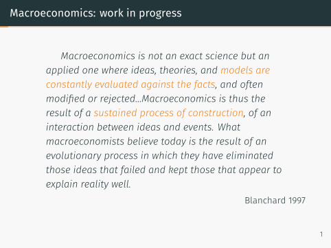
There is wide agreement about the major goals ofeconomic policy: high employment, stable prices, andrapid growth. There is less agreement that thesegoals are mutually compatible or, among those whoregard them as incompatible, about the terms atwhich they can and should be substituted for oneanother. There is least agreement about the role thatvarious instruments of policy can and should play inachieving the several goals.

Friedman 1968

2

Macroeconomics controversy

One view and school of thought, associated withKeynes, Keynesians and new Keynesians, is that theprivate economy is subject to co-ordination failuresthat can produce excessive levels of unemploymentand excessive fluctuations in real activity. The otherview, attributed to classical economists, and espousedby monetarists and equilibrium business cycletheorists, is that the private economy reaches as goodan equilibrium as is possible given government policy.

Fischer 1988

3

Keynesian perspective

Involuntary unemployment can exist and, without governmentassistance, any adjustment toward “full employment” is likelyto be slow and to involve cycles and overshoots, eitherbecause

• the economy has multiple equilibria, only one of whichinvolves full employment;

• there is only one equilibrium, but the economic system isunstable without policy.

4

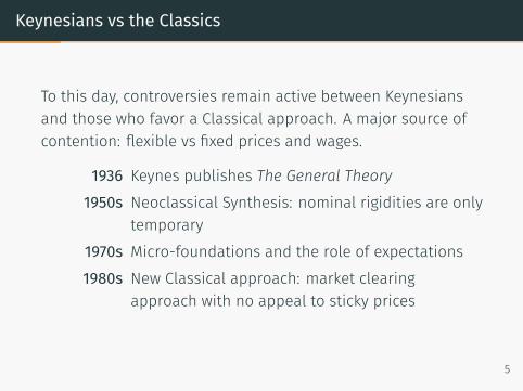
Keynesians vs the Classics

To this day, controversies remain active between Keynesiansand those who favor a Classical approach. A major source ofcontention: flexible vs fixed prices and wages.

1936 Keynes publishes The General Theory1950s Neoclassical Synthesis: nominal rigidities are only

temporary1970s Micro-foundations and the role of expectations1980s New Classical approach: market clearing

approach with no appeal to sticky prices

5

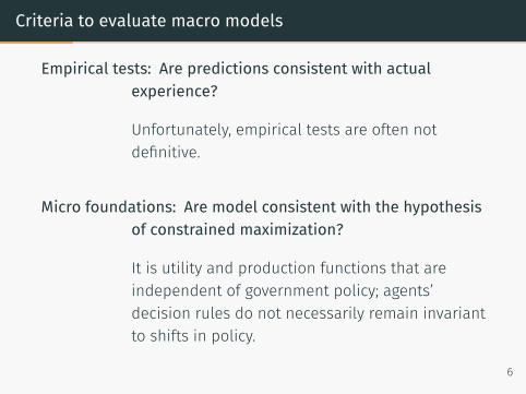
Criteria to evaluate macro models

Empirical tests: Are predictions consistent with actualexperience?

Unfortunately, empirical tests are often notdefinitive.

Micro foundations: Are model consistent with the hypothesisof constrained maximization?

It is utility and production functions that areindependent of government policy; agents’decision rules do not necessarily remain invariantto shifts in policy.

6

Two stages to making macro models

1. Derive the structural equations, which define the macromodel, by presenting a set of constrained maximizationexercises

2. Use the set of structural equations to derive the solutionor reduce-form equations and perform the counterfactualexercises.

Since the 1970s, the two stages are considered simultaneously:structural equations make reference to the properties of theoverall system (e.g. rational expectations).

7

The Classical model

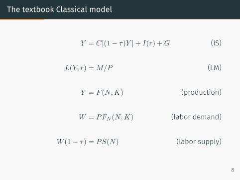
The textbook Classical model

Y = C[(1− τ)Y ] + I(r) +G (IS)

L(Y, r) = M/P (LM)

Y = F (N,K) (production)

W = PFN (N,K) (labor demand)

W (1− τ) = PS(N) (labor supply)

8

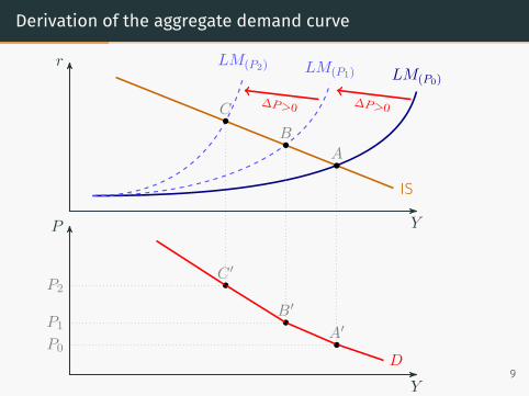
Derivation of the aggregate demand curve

r

Y

IS

LM(P0)

P

Y

A

A′P0

LM(P1)

B

B′P1

∆P>0

LM(P2)

C

C ′P2

∆P>0

D9

Classical dichotomy

There are five endogenous variables: Y,N, r, P,W .

• The real variables (N,Y ) are determined solely on thebasis of aggregate supply relationships (factor market andproduction function), while...

• the demand considerations (the IS and LM curves)determined the nominal variables (r,W,P ) residually.

10

Aggregate demand and supply curves

P

Y

D(M,G, τ)

S(K, τ) • Classical dichotomyfollows from the verticalS(K, τ)

• A policy ofbalanced-budgetreduction in the size ofgovernment makes sense:higher output and lowerprices can follow tax cuts.

11

The Classical Model

Y

N

W

N

Y

Y

P

Y

45◦

PFN

PSN1−τ

S

D1

D112

The Keynesian model

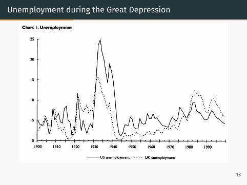
Unemployment during the Great Depression Britton Macroeconomics and history 107

Chart I. Unemployment

25 r

20

15

10

I ' I 1 Iv' I 1 I 1 I 1 I 1 I ■"!' 1 I 1 I ■ I 1 I 1 I 1 I 1 I ■ I 1 I 1 I ' I 1900 1910 1920 1930 1940 1950 I 960 1970 1980 1990

US unemployment UK unemployment

25 r

I 1 I 1 II 1 I 1 I 1 I 1 I '"V ' I ■ I ■ I 1 I ' I ■ I ■ I ■ I ' I ■ I 1900 1910 1920 1930 1940 1950 I 960 1970 1980 1990

US unemployment UK unemployment

Chart 2. Inflation

1900 1910 1920 1930 1940 1950 I 960 1970 1980 1990

US inflation UK inflation

1900 1910 1920 1930 1940 1950 I 960 1970 1980 1990

US inflation UK inflation

This content downloaded from 140.254.87.149 on Thu, 28 Jul 2016 06:21:50 UTCAll use subject to http://about.jstor.org/terms

13

The Great Depression

Country Depressionbegan

Recoverybegins

Industrial production% decline

USA 1929q3 1933q2 46.8UK 1930q1 1931q4 16.2Germany 1928q1 1932q3 41.8France 1930q2 1932q3 31.3Italy 1929q3 1933q1 33.0

Belgium 1929q3 1932q4 30.6Netherlands 1929q4 1933q2 37.4Denmark 1930q4 1933q2 16.5Sweden 1930q2 1932q3 10.3Czechoslovakia 1929q4 1932q3 40.4

Poland 1929q1 1933q2 46.6Canada 1929q2 1933q2 42.4Argentina 1929q2 1932q1 17.0Brazil 1928q3 1931q4 7.0Japan 1930q1 1932q3 8.5

Source: C. Romer (2004)14

Just wait for the storm to pass?

If, after the American civil war, the American dollarhad been stabilised and defined by law at 10 per centbelow its present value, it would be safe to assumethat [the quantity of money] and [the price level]would now be just 10 per cent greater than theyactually are and that the present values of [thevelocity of circulation and the reserve ratio] would beentirely unaffected. But this long run is a misleadingguide to current affairs. In the long run we are alldead. Economists set themselves too easy, toouseless, a task if in tempestuous seasons they canonly tell us that when the storm is long past theocean is flat again.

Keynes 1923, Tract on Monetary Reform15

Keynes and the Great Depression

• The history of modern macroeconomicsstarts with the publication of JohnMaynard Keynes’s General Theory ofEmployment, Interest, and Money in 1936.

• The General Theory is in fact businesscycle theory that emphasizes effectivedemand (aggregate demand): Effectivedemand determines output.

John MaynardKeynes

16

Keynes contributions

Keynes built the building blocks of modern macroeconomics:

• The relation of consumption, to income and the multipliereffects

• Liquidity preference in the demand for money thatexplains how monetary policy affect interest rates andaggregate demand

• The importance of expectations in affecting consumptionand investment; and shifts in expectations (animal spirits)behind shifts in demand and output

17

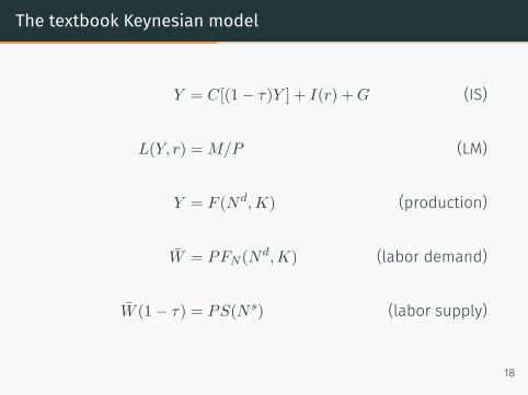
The textbook Keynesian model

Y = C[(1− τ)Y ] + I(r) +G (IS)

L(Y, r) = M/P (LM)

Y = F (Nd,K) (production)

W = PFN (Nd,K) (labor demand)

W (1− τ) = PS(N s) (labor supply)

18

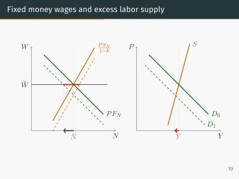
Fixed money wages and excess labor supply

W

N

PFN

PSN1−k

W

N

P

Y

S

D0

Y

D1

19

Unemployment in the Keynesian model

• Unemployment occurs in the Keynesian model because ofwage rigidity.

• It can be reduced by any of the following policies1. increasing government spending,2. increasing the money supply, or3. reducing the money wage

20

The Neoclassical Synthesis

The Neoclassical Synthesis

• By the 1950s, a consensus, called theneoclassical synthesis, had emerged.

• The IS-LM model, developed earlier byJohn Hicks and Alvin Hansen, was used toformalize Keynes’s ideas.

• Modigliani and Friedman independentlydeveloped the theory of consumptionthat emphasizes the importance ofexpectations in determining currentconsumption decision.

Franco Modigliani

Milton Friedman

21

The Neoclassical Synthesis (2)

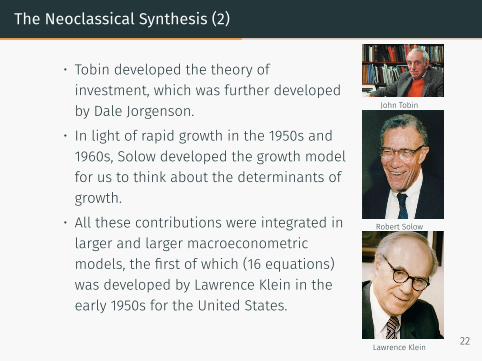
• Tobin developed the theory ofinvestment, which was further developedby Dale Jorgenson.

• In light of rapid growth in the 1950s and1960s, Solow developed the growth modelfor us to think about the determinants ofgrowth.

• All these contributions were integrated inlarger and larger macroeconometricmodels, the first of which (16 equations)was developed by Lawrence Klein in theearly 1950s for the United States.

John Tobin

Robert Solow

Lawrence Klein22

The Neoclassical Synthesis (3)

• The most impressive effort was the construction of theMPS model developed during the 1960s as an expandedversion of the IS-LM model, plus a Phillips curvemechanism.

• In the 1960s, there were heated debates between“Keynesians” and “monetarists”, centering around threeissues:

1. the effectiveness of monetary versus fiscal policy,2. the Phillips curve, and3. the role of policy.

• Keynes’s emphasis on fiscal rather than monetary policywas challenged by the opposite view of Friedman.

23

The Phillips curve

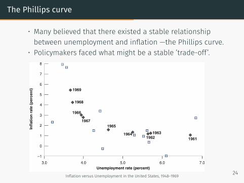
• Many believed that there existed a stable relationshipbetween unemployment and inflation —the Phillips curve.

• Policymakers faced what might be a stable ’trade-off’.

Inflation versus Unemployment in the United States, 1948–1969 24

Monetarism

• Friedman and Phelps also challenged theKeynesian view of a reliable trade-offbetween unemployment and inflation,even in the long run.

• In contrast to the Keynesians’ call for anactive role of policy, Friedman argued forthe use of simple rules, such as steadymoney growth.

• This debate on the role ofmacroeconomic policy has not beensettled.

Milton Friedman

Edmund Phelps

25

Good-by Phillips curve?

• The Phillips curve: view of economics as engineering; itbecame the centre piece of econometric models.

• It was, in subsequent years, to prove hopelessly unreliable

Inflation versus Unemployment in the United States, 1970–2010

26

The Rational Expectations Critique

The Rational Expectations Critique

• In the early 1970s, Lucas, Sargent and Barro led astrong attack against mainstream macroeconomics.

• Lucas and Sargent’s main argument was based onthree implications of rational expectations, all highlydamaging to Keynesian macroeconomics:

• Existing macroeconomic models could not be used todesign policy, known as the Lucas critique.

• With rational expectations, only unanticipatedchanges in money should affect output.

• Game theory, rather than optimal control in Keynesianmodels, was the right tool to design policy.

Robert Lucas

Thomas Sargent

Robert Barro

27

The Rational Expectations Critique (2)

• The role of rational expectations has been integratedin different markets:

• Hall showed that if consumers are foresighted, thenconsumption behavior became random walk.

• Dornbusch showed that the large swings in exchangerates under flexible exchange rates were fullyconsistent with rationality rather than the result ofspeculation by irrational investors

• Fischer and Taylor showed that, due to staggering ofwage and price decisions, the adjustment of pricesand wages in response to changes in unemploymentcan be slow even under rational expectations.

• By the end of the 1980s, the rational-expectationscritique had led to an overhaul of macroeconomics.

Rudiger Dornbusch

Stanley Fischer

John Taylor28

Keynesians vs Classical: The role of money

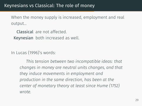
When the money supply is increased, employment and realoutput...

Classical are not affected.Keynesian both increased as well.

In Lucas (1996)’s words:

This tension between two incompatible ideas: thatchanges in money are neutral units changes, and thatthey induce movements in employment andproduction in the same direction, has been at thecenter of monetary theory at least since Hume (1752)wrote.

29

Estimating the effect of money on output

Suppose we estimate the relationship between output andmoney by

yt = y0 + α0mt + α1mt−1 + c1zt + c2zt−1 + ut

Here, systemic variations in the money supply affect output.

If central bank wants to reduce fluctuations in real output(assuming it forecasts that zt = 0) it sets the money supply to

mt = −α1

α0mt−1 −

c2α0

zt−1 + vt

= π1mt−1 + π2zt−1 + vt (policy rule)

30

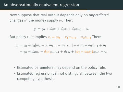
An observationally equivalent regression

Now suppose that real output depends only on unpredictedchanges in the money supply vt. Then:

yt = y0 + d0vt + d1zt + d2zt−1 + ut

But policy rule implies vt = mt − π1mt−1 − π2zt−1.Then:

yt = y0 + d0[mt − π1mt−1 − π2zt−1] + d1zt + d2zt−1 + ut

= y0 + d0mt − d0π1mt−1 + d1zt + (d2 − d0π2)zt−1 + ut

• Estimated parameters may depend on the policy rule.• Estimated regression cannot distinguish between the twocompeting hypothesis.

31

Lucas and rational expectations

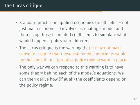
The Lucas critique

• Standard practice in applied economics (in all fields – notjust macroeconomics) involves estimating a model andthen using those estimated coefficients to simulate whatwould happen if policy were different.

• The Lucas critique is the warning that it may not makesense to assume that those estimated coefficients wouldbe the same if an alternative policy regime were in place.

• The only way we can respond to this warning is to havesome theory behind each of the model’s equations. Wecan then derive how (if at all) the coefficients depend onthe policy regime.

32

The role of expectations

• Early work in macroeconomics involved a bold simplifyingassumption – that economic agents have staticexpectations concerning the model’s endogenousvariables.

• Conflicting assumptions:• individuals took great pains to pursue a detailed planwhen deciding how much to consume and how to operatetheir firms.

• these same individuals were quite content to just presumethat many important variables that affect their decisionswill never change

• By 1970, macro theorists had come to regard thisapproach as unappealing.

33

Four approaches to modelling expectations

• Static expectations: Individuals are always surprised byany changes, and so they make systematic forecast errors.

• Adaptive expectations: Individuals forecast eachendogenous variable by assuming that the future valuewill be a weighted average of past values for that variable.

• Perfect foresight: Individuals are so adept at revising theirforecasts in the light of new information that they nevermake any forecast errors.

• Rational expectations: Individuals understand theprobability distributions of shocks affecting the economy,so their subjective expectations is consistent with themathematical expectation implied by the model.

34

DSGE, RBC, New Keynesian

Developments in Macroeconomics up to the 2009 Crisis

• From the late 1980s to the crisis, the new classicalsdeveloped the real business cycle (RBC) models based ontwo premises:

• Macroeconomic models should be constructed fromexplicit microfoundations.

• Most fluctuations until the 1970s were the results ofimperfections, of deviations of actual output from a slowlymoving potential level of output.

35

Developments in Macroeconomics up to the 2009 Crisis

• New Keynesians recognized rational expectations, butbelieved that much remained to be learned about thenature of market imperfections and their implications formacroeconomic fluctuations.

• Their work included studying the nature and implicationsof nominal rigidities, and the menu cost, and efficiencywages.

• Michael Woodford and Jordi Gali built the new Keynesianmodel that embodies utility and profit maximization,rational expectations, and nominal rigidities.

• Since the late 1980s, contributions to growth theory wentunder the name of new growth theory, led by Robert Lucasand Paul Romer.

36

DSGE: Dynamic stochastic general equilibrium

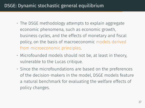
• The DSGE methodology attempts to explain aggregateeconomic phenomena, such as economic growth,business cycles, and the effects of monetary and fiscalpolicy, on the basis of macroeconomic models derivedfrom microeconomic principles.

• Microfounded models should not be, at least in theory,vulnerable to the Lucas critique.

• Since the microfoundations are based on the preferencesof the decision-makers in the model, DSGE models featurea natural benchmark for evaluating the welfare effects ofpolicy changes.

37

Components of a DSGE

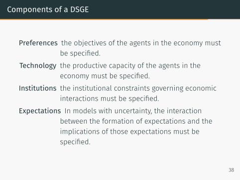
Preferences the objectives of the agents in the economy mustbe specified.

Technology the productive capacity of the agents in theeconomy must be specified.

Institutions the institutional constraints governing economicinteractions must be specified.

Expectations In models with uncertainty, the interactionbetween the formation of expectations and theimplications of those expectations must bespecified.

38

Models and questions

Basic DSGE models are based on three kinds of models:

• the Solow model• the Ramsey model• the overlapping generations model.

There are three kind of questions of interest:

• Transitional dynamics• Economic fluctuations that are caused by supply anddemand shocks.

• Implications of heterogeneous agents: incomedistribution.

39

Schools of DSGE modeling

At present two competing schools of thought form the bulk ofDSGE modeling:

RealBusinessCycle

theory builds on the neoclassical growth model(assumes flexible prices) to study how real shocksto the economy might cause business cyclefluctuations.

New-Keynesian

DSGE

models build on a structure similar to RBC models,but instead assume that prices are set bymonopolistically competitive firms, and cannot beinstantaneously and costlessly adjusted.

40

RBC: Real business cycle

During the years following the seminal papers of Kydland andPrescott (1982) and Prescott (1986), RBC theory provided themain framework for the analysis of economic fluctuations andbecame the core of macroeconomic theory.

The RBC revolution rested in three basic claims:

• The efficiency of business cycles.• The importance of technology shocks as a source ofeconomic fluctuation.

• The limited role of monetary factors.

41

The New Keynesian Model

The New Keynesian modelling approach combines the DSGEstructure characteristic of RBC models with assumptions thatdepart from those in classical monetary models:

• Monopolistic competition• Nominal rigidities• Short run non-neutrality of monetary policy

42

First Lessons for Macroeconomics after the Crisis

• The crisis reflects a major failure of macroeconomics torealize that a relatively small shock like the decrease inU.S. housing prices, could lead to a major financial andmacroeconomic global crisis.

• Much of the work to understand the crisis was carried outoutside macroeconomics, in the fields of finance orcorporate finance.

• Researchers have turned their attention to the financialsystem, the nature of macro financial linkages, andintegration of those pieces into large macroeconomicmodels.

43

References

Blanchard, Olivier (2017). Macroeconomics. 7th ed. Pearson.isbn: 978-0133780581.

Scarth, William (2014). Macroeconomics. The Development ofModern Methods for Policy Analysis. Edward ElgarPublishing Limited. isbn: 978-1-78195-388-4.

Snowdon, Brian and Howard R. Vane (2005). ModernMacroeconomics. Its Origins, Development and Current State.Edward Elgar Publishing Limited. isbn: 1-84542-208-2.

Walsh, Carl E. (2010). Monetary Theory and Policy. 3rd ed. MITPress. isbn: 978-0262-013772.

44