Embed Size (px)
Citation preview

Lecture 1: Introduction to Spatial Econometric
Professor: Mauricio Sarrias
Universidad Católica del Norte
September 7, 2017

1 Introduction to Spatial EconometricMandatory ReadingWhy do We Need Spatial EconometricSpatial Heterogeneity and DependenceSpatial Autocorrelation
2 Spatial Weight MatrixDefinitionWeights Based on BoundariesFrom Contiguity to the W MatrixWeights Based on DistanceRow StandardizationSpatial LagHigher-Order Spatial Neighbors
3 Examples of Weight Matrices in RCreating Contiguity NeighborsCreating Distance-Based
4 Testing for Spatial AutocorrelationIndicators of spatial associationMoran’s I
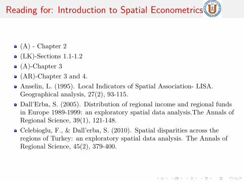
Reading for: Introduction to Spatial Econometrics
(A) - Chapter 2(LK)-Sections 1.1-1.2(A)-Chapter 3(AR)-Chapter 3 and 4.Anselin, L. (1995). Local Indicators of Spatial Association- LISA.Geographical analysis, 27(2), 93-115.Dall’Erba, S. (2005). Distribution of regional income and regional fundsin Europe 1989-1999: an exploratory spatial data analysis.The Annals ofRegional Science, 39(1), 121-148.Celebioglu, F., & Dall’erba, S. (2010). Spatial disparities across theregions of Turkey: an exploratory spatial data analysis. The Annals ofRegional Science, 45(2), 379-400.

1 Introduction to Spatial EconometricMandatory ReadingWhy do We Need Spatial EconometricSpatial Heterogeneity and DependenceSpatial Autocorrelation
2 Spatial Weight MatrixDefinitionWeights Based on BoundariesFrom Contiguity to the W MatrixWeights Based on DistanceRow StandardizationSpatial LagHigher-Order Spatial Neighbors
3 Examples of Weight Matrices in RCreating Contiguity NeighborsCreating Distance-Based
4 Testing for Spatial AutocorrelationIndicators of spatial associationMoran’s I

Why do We Need Spatial Econometric
Important aspect when studying spatial units (cities, regions, countries)
Potential relationships and interactions between them.Example: Modeling pollution:
Analyze regions as independent units?No, regions are spatially interrelated by ecological and economicinteractions.Existence of environmental externalities:
and increase in i’s pollution will affect the pollution in neighbors regions,but the impact will be lower for more distance regions.

Why do We Need Spatial Econometric
Important aspect when studying spatial units (cities, regions, countries)Potential relationships and interactions between them.
Example: Modeling pollution:
Analyze regions as independent units?No, regions are spatially interrelated by ecological and economicinteractions.Existence of environmental externalities:
and increase in i’s pollution will affect the pollution in neighbors regions,but the impact will be lower for more distance regions.

Why do We Need Spatial Econometric
Important aspect when studying spatial units (cities, regions, countries)Potential relationships and interactions between them.
Example: Modeling pollution:Analyze regions as independent units?
No, regions are spatially interrelated by ecological and economicinteractions.Existence of environmental externalities:
and increase in i’s pollution will affect the pollution in neighbors regions,but the impact will be lower for more distance regions.

Why do We Need Spatial Econometric
Important aspect when studying spatial units (cities, regions, countries)Potential relationships and interactions between them.
Example: Modeling pollution:Analyze regions as independent units?No, regions are spatially interrelated by ecological and economicinteractions.
Existence of environmental externalities:
and increase in i’s pollution will affect the pollution in neighbors regions,but the impact will be lower for more distance regions.

Why do We Need Spatial Econometric
Important aspect when studying spatial units (cities, regions, countries)Potential relationships and interactions between them.
Example: Modeling pollution:Analyze regions as independent units?No, regions are spatially interrelated by ecological and economicinteractions.Existence of environmental externalities:
and increase in i’s pollution will affect the pollution in neighbors regions,but the impact will be lower for more distance regions.

Figure: Environmental Externalities
R1 R2 R3 R4 R5

Distance Matters
Key Point:First law of geography of Waldo Tobler: “everything is related to everythingelse”, but near things are more related than distant things
This first law is the foundation of the fundamental concepts of spatialdependence and spatial autocorrelation.

1 Introduction to Spatial EconometricMandatory ReadingWhy do We Need Spatial EconometricSpatial Heterogeneity and DependenceSpatial Autocorrelation
2 Spatial Weight MatrixDefinitionWeights Based on BoundariesFrom Contiguity to the W MatrixWeights Based on DistanceRow StandardizationSpatial LagHigher-Order Spatial Neighbors
3 Examples of Weight Matrices in RCreating Contiguity NeighborsCreating Distance-Based
4 Testing for Spatial AutocorrelationIndicators of spatial associationMoran’s I

Why do We Need Spatial Econometric
Spatial econometric deals with spatial effects(I) Spatial heterogeneity
(II) Spatial dependence
Definition (Spatial heterogeneity)Spatial heterogeneity relates to a differentiation of the effects of space over thesample units. Formally, for spatial unit i:
yi = f(xi)i + εi =⇒ yi = βixi + εi
Lack of stability over the geographical space.
Definition (Spatial dependence)What happens in i depends on what happens in j. Formally,
yi = f(yi, yj) + εi,∀i 6= j.

Why do We Need Spatial Econometric
Spatial econometric deals with spatial effects
(I) Spatial heterogeneity
(II) Spatial dependence
Definition (Spatial heterogeneity)Spatial heterogeneity relates to a differentiation of the effects of space over thesample units. Formally, for spatial unit i:
yi = f(xi)i + εi =⇒ yi = βixi + εi
Lack of stability over the geographical space.
Definition (Spatial dependence)What happens in i depends on what happens in j. Formally,
yi = f(yi, yj) + εi,∀i 6= j.
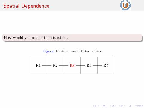
Spatial Dependence
How would you model this situation?
Figure: Environmental Externalities
R1 R2 R3 R4 R5

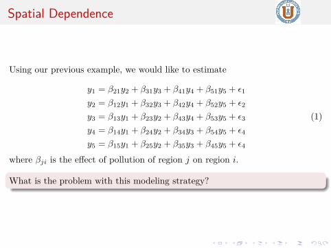
Spatial Dependence
Using our previous example, we would like to estimate
y1 = β21y2 + β31y3 + β41y4 + β51y5 + ε1
y2 = β12y1 + β32y3 + β42y4 + β52y5 + ε2
y3 = β13y1 + β23y2 + β43y4 + β53y5 + ε3
y4 = β14y1 + β24y2 + β34y3 + β54y5 + ε4
y5 = β15y1 + β25y2 + β35y3 + β45y5 + ε4
(1)
where βji is the effect of pollution of region j on region i.
What is the problem with this modeling strategy?

Spatial Dependence
Under standard econometric modeling, it is impossible to model spatialdependency.

1 Introduction to Spatial EconometricMandatory ReadingWhy do We Need Spatial EconometricSpatial Heterogeneity and DependenceSpatial Autocorrelation
2 Spatial Weight MatrixDefinitionWeights Based on BoundariesFrom Contiguity to the W MatrixWeights Based on DistanceRow StandardizationSpatial LagHigher-Order Spatial Neighbors
3 Examples of Weight Matrices in RCreating Contiguity NeighborsCreating Distance-Based
4 Testing for Spatial AutocorrelationIndicators of spatial associationMoran’s I

Spatial Autocorrelation
Autocorrelation =⇒ the correlation of a variables with itself
Time series: the values of a variable at time t depends on the value of thesame variable at time t− 1.Space: the correlation between the value of the variable at two differentlocations.
Definition (Spatial Autocorrelation)Correlation between the same attribute at two (or more) differentlocations.Coincidence of values similarity with location similarity.Under spatial dependency it is not possible to change the location of thevalues of certain variable without affecting the information in the sample.It can be positive and negative.

Spatial Autocorrelation
Autocorrelation =⇒ the correlation of a variables with itselfTime series: the values of a variable at time t depends on the value of thesame variable at time t− 1.
Space: the correlation between the value of the variable at two differentlocations.
Definition (Spatial Autocorrelation)Correlation between the same attribute at two (or more) differentlocations.Coincidence of values similarity with location similarity.Under spatial dependency it is not possible to change the location of thevalues of certain variable without affecting the information in the sample.It can be positive and negative.

Spatial Autocorrelation
Autocorrelation =⇒ the correlation of a variables with itselfTime series: the values of a variable at time t depends on the value of thesame variable at time t− 1.Space: the correlation between the value of the variable at two differentlocations.
Definition (Spatial Autocorrelation)Correlation between the same attribute at two (or more) differentlocations.Coincidence of values similarity with location similarity.Under spatial dependency it is not possible to change the location of thevalues of certain variable without affecting the information in the sample.It can be positive and negative.

Spatial Autocorrelation
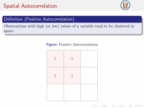
Definition (Positive Autocorrelation)Observations with high (or low) values of a variable tend to be clustered inspace.
Figure: Positive Autocorrelation
1 1
1 1
Spatial Autocorrelation
Definition (Positive Autocorrelation)Observations with high (or low) values of a variable tend to be clustered inspace.
Figure: Positive Autocorrelation
1 1
1 1

Spatial Autocorrelation
Definition (Negative Autocorrelation)Locations tend to be surrounded by neighbors having very dissimilar values.
Figure: Negative Autocorrelation
1 1
1
1 1

Spatial Autocorrelation
Definition (Negative Autocorrelation)Locations tend to be surrounded by neighbors having very dissimilar values.
Figure: Negative Autocorrelation
1 1
1
1 1

Spatial Autocorrelation: Another ExamplePositive Spatial Autocorrelation Negative Spatial Autocorrelation

Spatial Autocorrelation
Definition (Spatial Randomness)When none of the two situations occurs.

Spatial Autocorrelation
Two main sources of spatial autocorrelation (Anselin, 1988):Measurement errors.Importance of Space.
The second source is of much more interest.
Why the space matters?
The essence of regional sciences and new economic geography is thatlocation and distance matter.What is observed at one point is determined by what happen elsewhere inthe system.

First Law of Geography Again
Tobler’s First Law of GeographyEverything depends on everything else, but closer things more so
Important ideas:
Existence of Spatial Dependence.Structure of Spatial Dependence
Distance decay.Closeness = Similarities.

First Law of Geography Again
Tobler’s First Law of GeographyEverything depends on everything else, but closer things more so
Important ideas:Existence of Spatial Dependence.
Structure of Spatial Dependence
Distance decay.Closeness = Similarities.
First Law of Geography Again
Tobler’s First Law of GeographyEverything depends on everything else, but closer things more so
Important ideas:Existence of Spatial Dependence.Structure of Spatial Dependence
Distance decay.Closeness = Similarities.

First Law of Geography Again
Tobler’s First Law of GeographyEverything depends on everything else, but closer things more so
Important ideas:Existence of Spatial Dependence.Structure of Spatial Dependence
Distance decay.
Closeness = Similarities.

First Law of Geography Again
Tobler’s First Law of GeographyEverything depends on everything else, but closer things more so
Important ideas:Existence of Spatial Dependence.Structure of Spatial Dependence
Distance decay.Closeness = Similarities.

1 Introduction to Spatial EconometricMandatory ReadingWhy do We Need Spatial EconometricSpatial Heterogeneity and DependenceSpatial Autocorrelation
2 Spatial Weight MatrixDefinitionWeights Based on BoundariesFrom Contiguity to the W MatrixWeights Based on DistanceRow StandardizationSpatial LagHigher-Order Spatial Neighbors
3 Examples of Weight Matrices in RCreating Contiguity NeighborsCreating Distance-Based
4 Testing for Spatial AutocorrelationIndicators of spatial associationMoran’s I

Spatial Weight Matrix
One crucial issue in spatial econometric is the problem of formallyincorporating spatial dependence into the model.
Question?What would be a good criteria to define closeness in space? Or, in otherwords, how to determine which other units in the system influence the oneunder consideration?
Spatial Weight Matrix
The device typically used in spatial analysis is the so-called spatial weightmatrix, or simply W matrix.Impose a structure in terms of what are the neighbors for each location.Assigns weights that measure the intensity of the relationship among pairof spatial units.Not necessarily symmetric.
Spatial Weight Matrix
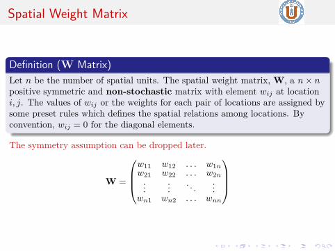
Definition (W Matrix)Let n be the number of spatial units. The spatial weight matrix, W, a n× npositive symmetric and non-stochastic matrix with element wij at locationi, j. The values of wij or the weights for each pair of locations are assigned bysome preset rules which defines the spatial relations among locations. Byconvention, wij = 0 for the diagonal elements.
The symmetry assumption can be dropped later.
W =
w11 w12 . . . w1nw21 w22 . . . w2n...
.... . .
...wn1 wn2 . . . wnn

Spatial Weight Matrix
Two main approaches:1 Contiguity.2 Based on distance

1 Introduction to Spatial EconometricMandatory ReadingWhy do We Need Spatial EconometricSpatial Heterogeneity and DependenceSpatial Autocorrelation
2 Spatial Weight MatrixDefinitionWeights Based on BoundariesFrom Contiguity to the W MatrixWeights Based on DistanceRow StandardizationSpatial LagHigher-Order Spatial Neighbors
3 Examples of Weight Matrices in RCreating Contiguity NeighborsCreating Distance-Based
4 Testing for Spatial AutocorrelationIndicators of spatial associationMoran’s I

Weights Based on Boundaries
The availability of polygon or lattice data permits the construction ofcontiguity-based spatial weight matrices. A typical specification of thecontiguity relationship in the spatial weight matrix is
wij ={
1 if i and j are contiguous0 if i and j are not contiguous
(2)
1 Binary Contiguity:Rook criterion (Common Border)Bishop criterion (Common Vertex)Queen criterion (Either common border or vertex)

Rook Contiguity
How are the neighbors of region 5?
Figure: Rook Contiguity
1 2 3
4 5 6
7 8 9

Rook Contiguity
Figure: Rook Contiguity
1 2 3
4 5 6
7 8 9
Common border: 2, 4, 5, 6

Rook Contiguity
Figure: Rook Contiguity
1 2 3
4 5 6
7 8 9
Common border: 2, 4, 5, 6

Bishop Contiguity
Figure: Bishop Contiguity
1 2 3
4 5 6
7 8 9
Common vertex: 1, 3, 7, 9

Bishop Contiguity
Figure: Bishop Contiguity
1 2 3
4 5 6
7 8 9
Common vertex: 1, 3, 7, 9

Queen Contiguity
Figure: Queen Contiguity
1 2 3
4 5 6
7 8 9
Common vertex and border: 1, 2, 3, 4, 6, 7, 8, 9.

Queen Contiguity
Figure: Queen Contiguity
1 2 3
4 5 6
7 8 9
Common vertex and border: 1, 2, 3, 4, 6, 7, 8, 9.

1 Introduction to Spatial EconometricMandatory ReadingWhy do We Need Spatial EconometricSpatial Heterogeneity and DependenceSpatial Autocorrelation
2 Spatial Weight MatrixDefinitionWeights Based on BoundariesFrom Contiguity to the W MatrixWeights Based on DistanceRow StandardizationSpatial LagHigher-Order Spatial Neighbors
3 Examples of Weight Matrices in RCreating Contiguity NeighborsCreating Distance-Based
4 Testing for Spatial AutocorrelationIndicators of spatial associationMoran’s I

Rook Contiguity
1 2 3
4 5 6
7 8 9
W =
0 1 0 1 0 0 0 0 01 0 1 0 1 0 0 0 00 1 0 0 0 1 0 0 01 0 0 0 1 0 1 0 00 1 0 1 0 1 0 1 00 0 1 0 1 0 0 0 10 0 0 1 0 0 0 1 00 0 0 0 1 0 1 0 10 0 0 0 0 1 0 1 0

Bishop Contiguity
1 2 3
4 5 6
7 8 9
W =
0 0 0 0 1 0 0 0 00 0 0 1 0 1 0 0 00 0 0 0 1 0 0 0 00 1 0 0 0 0 0 1 01 0 1 0 0 0 1 0 10 1 0 0 0 0 0 1 00 0 0 0 1 0 0 0 00 0 0 1 0 1 0 0 00 0 0 0 1 0 0 0 0

1 Introduction to Spatial EconometricMandatory ReadingWhy do We Need Spatial EconometricSpatial Heterogeneity and DependenceSpatial Autocorrelation
2 Spatial Weight MatrixDefinitionWeights Based on BoundariesFrom Contiguity to the W MatrixWeights Based on DistanceRow StandardizationSpatial LagHigher-Order Spatial Neighbors
3 Examples of Weight Matrices in RCreating Contiguity NeighborsCreating Distance-Based
4 Testing for Spatial AutocorrelationIndicators of spatial associationMoran’s I

W based on distance
Weights may be also defined as a function of the distance between regioni and j, dij .dij is usually computed as the distance between their centroids (or otherimportant unit).Let xi an xj be the longitud and yi and yj the latitude coordinates forregion i and j, respectively:
Distance Metric
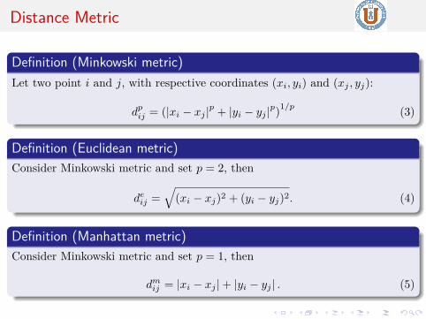
Definition (Minkowski metric)Let two point i and j, with respective coordinates (xi, yi) and (xj , yj):
dpij = (|xi − xj |p + |yi − yj |p)1/p (3)
Definition (Euclidean metric)Consider Minkowski metric and set p = 2, then
deij =
√(xi − xj)2 + (yi − yj)2. (4)
Definition (Manhattan metric)Consider Minkowski metric and set p = 1, then
dmij = |xi − xj |+ |yi − yj | . (5)

Distance Metric
Euclidean distance is not necessarily the shortest distance if you take intoaccount the curvature of the earth.
Definition (Great Circle Distance)Let two point i and j, with respective coordinates (xi, yi) and (xj , yj):
dcdij = r × arccos−1 [cos |xi − xj | cos yi cos yj + sin yi sin yj ] (6)
where r is the Earth’s radius. The arc distance is obtained in miles withr = 3959 and in kilometers with r = 6371.

W based on distance
Inverse distance:
wij ={
1dαij
if i 6= j
0 if i = j(7)
Typically, α = 1 or α = 2.Negative exponential model:
wij = exp(−dij
α
)(8)

W based on distance
k-nearest neighbors: We explicitly limit the number of neighbors.
wij ={
1 if centroid of j is one of the k nearest centroids to that of i0 otherwise
(9)Threshold Distance (Distance Band Weights): In contrast to thek-nearest neighbors method, the threshold distance specifies that anregion i is neighbor of j if the distance between them is less than aspecified maximum distance:
wij ={
1 if 0 ≤ dij ≤ dmax
0 if dij > dmax
(10)
To avoid isolates that would result from too stringent a critical distance,the distance must be chosen such that each location has at least oneneighbor. Such a distance conforms to a max-min criterion, i.e., it is thelargest of the nearest neighbor distances.

1 Introduction to Spatial EconometricMandatory ReadingWhy do We Need Spatial EconometricSpatial Heterogeneity and DependenceSpatial Autocorrelation
2 Spatial Weight MatrixDefinitionWeights Based on BoundariesFrom Contiguity to the W MatrixWeights Based on DistanceRow StandardizationSpatial LagHigher-Order Spatial Neighbors
3 Examples of Weight Matrices in RCreating Contiguity NeighborsCreating Distance-Based
4 Testing for Spatial AutocorrelationIndicators of spatial associationMoran’s I

Row standardization
W’s are used to compute weighted averages in which more weight isplaced on nearby observations than on distant observations.
The elements of a row-standardized weights matrix equal
wsij = wij∑
j wij.
This ensures that all weights are between 0 and 1 and facilities theinterpretation of operation with the weights matrix as an averaging ofneighboring values.Under row-standardization, the element of each row sum to unity.The row-standardized weights matrix also ensures that the spatialparameter in many spatial stochastic processes are comparable betweenmodels.Under row-standardization the matrices are not longer symmetric!.

Row standardization
W’s are used to compute weighted averages in which more weight isplaced on nearby observations than on distant observations.The elements of a row-standardized weights matrix equal
wsij = wij∑
j wij.
This ensures that all weights are between 0 and 1 and facilities theinterpretation of operation with the weights matrix as an averaging ofneighboring values.
Under row-standardization, the element of each row sum to unity.The row-standardized weights matrix also ensures that the spatialparameter in many spatial stochastic processes are comparable betweenmodels.Under row-standardization the matrices are not longer symmetric!.

Row standardization
W’s are used to compute weighted averages in which more weight isplaced on nearby observations than on distant observations.The elements of a row-standardized weights matrix equal
wsij = wij∑
j wij.
This ensures that all weights are between 0 and 1 and facilities theinterpretation of operation with the weights matrix as an averaging ofneighboring values.Under row-standardization, the element of each row sum to unity.
The row-standardized weights matrix also ensures that the spatialparameter in many spatial stochastic processes are comparable betweenmodels.Under row-standardization the matrices are not longer symmetric!.

Row standardization
W’s are used to compute weighted averages in which more weight isplaced on nearby observations than on distant observations.The elements of a row-standardized weights matrix equal
wsij = wij∑
j wij.
This ensures that all weights are between 0 and 1 and facilities theinterpretation of operation with the weights matrix as an averaging ofneighboring values.Under row-standardization, the element of each row sum to unity.The row-standardized weights matrix also ensures that the spatialparameter in many spatial stochastic processes are comparable betweenmodels.
Under row-standardization the matrices are not longer symmetric!.

Row standardization
W’s are used to compute weighted averages in which more weight isplaced on nearby observations than on distant observations.The elements of a row-standardized weights matrix equal
wsij = wij∑
j wij.
This ensures that all weights are between 0 and 1 and facilities theinterpretation of operation with the weights matrix as an averaging ofneighboring values.Under row-standardization, the element of each row sum to unity.The row-standardized weights matrix also ensures that the spatialparameter in many spatial stochastic processes are comparable betweenmodels.Under row-standardization the matrices are not longer symmetric!.

Row standardization
The row-standardized matrix is also known in the literature as therow-stochastic matrix:
Definition (Row-stochastic Matrix)A real n× n matrix A is called Markov matrix, or row-stochastic matrixif
1 aij ≥ 0 for 1 ≤ i, j ≤ n;2∑n
j=1 aij = 1 for 1 ≤ i ≤ n
An important characteristic of the row-stochastic matrix is related to its eigenvalues:
Theorem (Eigenvalues of row-stochastic Matrix)
Every eigenvalue ωi of a row-stochastic Matrix satisfies |ω| ≤ 1
Therefore, the eigenvalues of the row-stochastic (i.e., row-normalized, rowstandardized or Markov) neighborhood matrix Ws are in the range [−1,+1].

1 Introduction to Spatial EconometricMandatory ReadingWhy do We Need Spatial EconometricSpatial Heterogeneity and DependenceSpatial Autocorrelation
2 Spatial Weight MatrixDefinitionWeights Based on BoundariesFrom Contiguity to the W MatrixWeights Based on DistanceRow StandardizationSpatial LagHigher-Order Spatial Neighbors
3 Examples of Weight Matrices in RCreating Contiguity NeighborsCreating Distance-Based
4 Testing for Spatial AutocorrelationIndicators of spatial associationMoran’s I

Spatial Lag
The spatial lag operator takes the form yL = Wy with dimension n× 1, whereeach element is given by yLi =
∑j wijyj , i.e., a weighted average of the y
values in the neighbor of i.For example:
Wy =(
0 1 01 0 10 1 0
)(105030
)=(
5010 + 30
50
)(11)
Using a row-standardized weight matrix:
Wsy =(
0 1 00.5 0 0.50 1 0
)(105030
)=(
505 + 15
50
)(12)
Therefore, when W is standardized, each element (Wy)i is interpreted as aweighted average of the y values for i’s neighbors.

1 Introduction to Spatial EconometricMandatory ReadingWhy do We Need Spatial EconometricSpatial Heterogeneity and DependenceSpatial Autocorrelation
2 Spatial Weight MatrixDefinitionWeights Based on BoundariesFrom Contiguity to the W MatrixWeights Based on DistanceRow StandardizationSpatial LagHigher-Order Spatial Neighbors
3 Examples of Weight Matrices in RCreating Contiguity NeighborsCreating Distance-Based
4 Testing for Spatial AutocorrelationIndicators of spatial associationMoran’s I

Higher-Order Neighbors
How to define higher-order neighbors?We might be interested in the neighbors of the neighbors of spatial unit i.
We define the higher-order spatial weigh matrix l as Wl.Spatial weight of order l = 2 is given by W2 = WW.Spatial weight of order l = 3 is given by W3 = WWW.
As an illustration consider the following structure for our previousexample:
W =
0 1 0 0 01 0 1 0 00 1 0 1 00 0 1 0 10 0 0 1 0
(13)

Higher-Order NeighborsThen W2 = WW based on the 5× 5 first-order contiguity matrix W from(13) is:
W2 =
1 0 1 0 00 2 0 1 01 0 2 0 10 1 0 2 00 0 1 0 1
(14)
Figure: Higher-Order Neighbors
R1 R2 R3 R4 R5
R1 R2 R3 R4 R5

1 Introduction to Spatial EconometricMandatory ReadingWhy do We Need Spatial EconometricSpatial Heterogeneity and DependenceSpatial Autocorrelation
2 Spatial Weight MatrixDefinitionWeights Based on BoundariesFrom Contiguity to the W MatrixWeights Based on DistanceRow StandardizationSpatial LagHigher-Order Spatial Neighbors
3 Examples of Weight Matrices in RCreating Contiguity NeighborsCreating Distance-Based
4 Testing for Spatial AutocorrelationIndicators of spatial associationMoran’s I

Examples in R
Creating spatial weight matrices by hand is tedious (and almostimpossible).However, there exists several statistical software that allow us to createthem in a very simply fashion.First, we need the shape file, which has geographical information:
It is a digital vector storage for storing geometric location and associatedattribute information
Mandatory files:.shp: shape format; the feature geometry itself,.shx: shape index format; a positional index of the feature geometry toallow seeking forwards and backwards quickly,.dbf: attribute format; columnar attributes for each shape, in dBase IVformat.
Examples in R
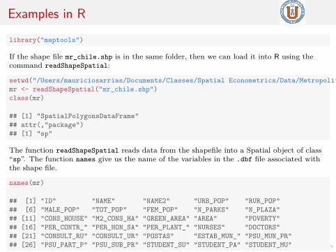
library("maptools")
If the shape file mr_chile.shp is in the same folder, then we can load it into R using thecommand readShapeSpatial:
setwd("/Users/mauriciosarrias/Documents/Classes/Spatial Econometrics/Data/MetropolitanRegion")mr <- readShapeSpatial("mr_chile.shp")class(mr)
## [1] "SpatialPolygonsDataFrame"## attr(,"package")## [1] "sp"
The function readShapeSpatial reads data from the shapefile into a Spatial object of class“sp”. The function names give us the name of the variables in the .dbf file associated withthe shape file.
names(mr)
## [1] "ID" "NAME" "NAME2" "URB_POP" "RUR_POP"## [6] "MALE_POP" "TOT_POP" "FEM_POP" "N_PARKS" "N_PLAZA"## [11] "CONS_HOUSE" "M2_CONS_HA" "GREEN_AREA" "AREA" "POVERTY"## [16] "PER_CONTR_" "PER_HON_SA" "PER_PLANT_" "NURSES" "DOCTORS"## [21] "CONSULT_RU" "CONSULT_UR" "POSTAS" "ESTAB_MUN_" "PSU_MUN_PR"## [26] "PSU_PART_P" "PSU_SUB_PR" "STUDENT_SU" "STUDENT_PA" "STUDENT_MU"

Examples in R
plot(mr, main = "Metropolitan Region-Chile", axes = TRUE)
−71.5 −71.0 −70.5 −70.0
−34
.5−
34.0
−33
.5−
33.0
Metropolitan Region−Chile
W in R
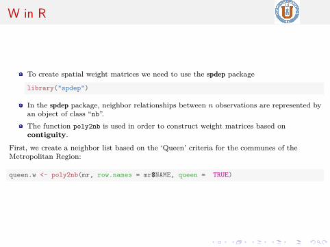
To create spatial weight matrices we need to use the spdep package
library("spdep")
In the spdep package, neighbor relationships between n observations are represented byan object of class “nb”.The function poly2nb is used in order to construct weight matrices based oncontiguity.
First, we create a neighbor list based on the ‘Queen’ criteria for the communes of theMetropolitan Region:
queen.w <- poly2nb(mr, row.names = mr$NAME, queen = TRUE)

W in R
summary(queen.w)
## Neighbour list object:## Number of regions: 52## Number of nonzero links: 292## Percentage nonzero weights: 10.79882## Average number of links: 5.615385## Link number distribution:#### 2 3 4 5 6 7 8 9 10 12## 3 2 7 15 10 10 2 1 1 1## 3 least connected regions:## Tiltil San Pedro Maria Pinto with 2 links## 1 most connected region:## San Bernardo with 12 links

W in RTo transform the list into an actual matrix W, we can use the function nb2listw:
queen.wl <- nb2listw(queen.w, style = "W")summary(queen.wl)
## Characteristics of weights list object:## Neighbour list object:## Number of regions: 52## Number of nonzero links: 292## Percentage nonzero weights: 10.79882## Average number of links: 5.615385## Link number distribution:#### 2 3 4 5 6 7 8 9 10 12## 3 2 7 15 10 10 2 1 1 1## 3 least connected regions:## Tiltil San Pedro Maria Pinto with 2 links## 1 most connected region:## San Bernardo with 12 links#### Weights style: W## Weights constants summary:## n nn S0 S1 S2## W 52 2704 52 19.76751 216.466

W in R
Now, we construct a binary matrix using the Rook criteria:
# Rook Wrook.w <- poly2nb(mr, row.names = mr$NAME, queen = FALSE)summary(rook.w)
## Neighbour list object:## Number of regions: 52## Number of nonzero links: 272## Percentage nonzero weights: 10.05917## Average number of links: 5.230769## Link number distribution:#### 2 3 4 5 6 7 8 9 10## 3 3 12 16 7 6 2 1 2## 3 least connected regions:## Tiltil San Pedro Maria Pinto with 2 links## 2 most connected regions:## Santiago San Bernardo with 10 links

W in RFinally, we can plot the weight matrices using the following set of commands.
# Plot Queen and Rook W Matricesplot(mr, border = "grey")plot(queen.w, coordinates(mr), add = TRUE, col = "red")plot(rook.w, coordinates(mr), add = TRUE, col = "yellow")

1 Introduction to Spatial EconometricMandatory ReadingWhy do We Need Spatial EconometricSpatial Heterogeneity and DependenceSpatial Autocorrelation
2 Spatial Weight MatrixDefinitionWeights Based on BoundariesFrom Contiguity to the W MatrixWeights Based on DistanceRow StandardizationSpatial LagHigher-Order Spatial Neighbors
3 Examples of Weight Matrices in RCreating Contiguity NeighborsCreating Distance-Based
4 Testing for Spatial AutocorrelationIndicators of spatial associationMoran’s I

W in RFirst, we extract coordinates: We now construct spatial weight matrices using the k-nearestneighbors criteria.
# K-neighborscoords <- coordinates(mr) # coordinates of centroidshead(coords, 5) # show coordinates
## [,1] [,2]## 0 -70.65599 -33.45406## 1 -70.71742 -33.50027## 2 -70.74504 -33.42278## 3 -70.67735 -33.38372## 4 -70.67640 -33.56294
k1neigh <- knearneigh(coords, k = 1, longlat = TRUE) # 1-nearest neighbork2neigh <- knearneigh(coords, k = 2, longlat = TRUE) # 2-nearest neighbor
The function coords extract the spatial coordinates from the shape file, whereas thefunction knearneigh return a matrix with the indices of points belonging to the set ofthe k-nearest neighbors of each other.The argument k indicates the number of nearest neighbors to be returned.If point coordinates are longitude-latitude decimal degrees, then distances aremeasured in kilometers if longlat = TRUE, if TRUE great circle distances are used.objects k1neigh and k2neigh are of class knn.

W in RWeight matrices based on inverse distance can be computed in the following way:
# Inverse weight matrixdist.mat <- as.matrix(dist(coords, method = "euclidean"))dist.mat[1:5, 1:5]
## 0 1 2 3 4## 0 0.00000000 0.07687010 0.09438408 0.07350782 0.11078109## 1 0.07687010 0.00000000 0.08226867 0.12324109 0.07489489## 2 0.09438408 0.08226867 0.00000000 0.07814455 0.15606360## 3 0.07350782 0.12324109 0.07814455 0.00000000 0.17922003## 4 0.11078109 0.07489489 0.15606360 0.17922003 0.00000000
dist.mat.inv <- 1 / dist.mat # 1 / d_{ij}diag(dist.mat.inv) <- 0 # 0 in the diagonaldist.mat.inv[1:5, 1:5]
## 0 1 2 3 4## 0 0.000000 13.008960 10.595007 13.603994 9.026811## 1 13.008960 0.000000 12.155295 8.114177 13.352046## 2 10.595007 12.155295 0.000000 12.796797 6.407644## 3 13.603994 8.114177 12.796797 0.000000 5.579733## 4 9.026811 13.352046 6.407644 5.579733 0.000000

W in R
# Standardized inverse weight matrixdist.mat.inve <- mat2listw(dist.mat.inv, style = "W", row.names = mr$NAME)summary(dist.mat.inve)
## Characteristics of weights list object:## Neighbour list object:## Number of regions: 52## Number of nonzero links: 2652## Percentage nonzero weights: 98.07692## Average number of links: 51## Link number distribution:#### 51## 52## 52 least connected regions:## Santiago Cerillos Cerro Navia Conchali El Bosque Estacion Central La Cisterna La Florida La Granja La Pintana La Reina Lo Espejo Lo Prado Macul Nunoa Pedro Aguirre Cerda Penalolen Providencia Quinta Normal Recoleta Renca San Joaquin San Miguel San Ramon Independencia Puente Alto Las Condes Vitacura Quilicura Huechuraba Maipu Pudahuel San Bernardo Tiltil Lampa Colina Lo Barnechea Pirque Paine Buin Alhue Melipilla San Pedro Maria Pinto Curacavi Penaflor Calera de Tango Padre Hurtado El Monte Talagante Isla de Maipo San Jose de Maipo with 51 links## 52 most connected regions:## Santiago Cerillos Cerro Navia Conchali El Bosque Estacion Central La Cisterna La Florida La Granja La Pintana La Reina Lo Espejo Lo Prado Macul Nunoa Pedro Aguirre Cerda Penalolen Providencia Quinta Normal Recoleta Renca San Joaquin San Miguel San Ramon Independencia Puente Alto Las Condes Vitacura Quilicura Huechuraba Maipu Pudahuel San Bernardo Tiltil Lampa Colina Lo Barnechea Pirque Paine Buin Alhue Melipilla San Pedro Maria Pinto Curacavi Penaflor Calera de Tango Padre Hurtado El Monte Talagante Isla de Maipo San Jose de Maipo with 51 links#### Weights style: W## Weights constants summary:## n nn S0 S1 S2## W 52 2704 52 2.902384 214.3332

W in R
Queen 1−Neigh
2−Neigh Inverse Distance
1 Introduction to Spatial EconometricMandatory ReadingWhy do We Need Spatial EconometricSpatial Heterogeneity and DependenceSpatial Autocorrelation
2 Spatial Weight MatrixDefinitionWeights Based on BoundariesFrom Contiguity to the W MatrixWeights Based on DistanceRow StandardizationSpatial LagHigher-Order Spatial Neighbors
3 Examples of Weight Matrices in RCreating Contiguity NeighborsCreating Distance-Based
4 Testing for Spatial AutocorrelationIndicators of spatial associationMoran’s I

Global Autocorrelation
Indicators of spatial association1 Global Autocorrelation2 Local Autocorrelation
Definition (Global Autocorrelation)It is a measure of overall clustering in the data. It yields only one statistic tosummarize the whole study area (Homogeneity).
1 Moran’s I.2 Gery’s C.3 Getis and Ord’s G(d)
Definition (Local Autocorrelation)A measure of spatial autocorrelation for each individual location.
Local Indices for spatial Spatial Analysis (LISA)
1 Introduction to Spatial EconometricMandatory ReadingWhy do We Need Spatial EconometricSpatial Heterogeneity and DependenceSpatial Autocorrelation
2 Spatial Weight MatrixDefinitionWeights Based on BoundariesFrom Contiguity to the W MatrixWeights Based on DistanceRow StandardizationSpatial LagHigher-Order Spatial Neighbors
3 Examples of Weight Matrices in RCreating Contiguity NeighborsCreating Distance-Based
4 Testing for Spatial AutocorrelationIndicators of spatial associationMoran’s I

Moran’s I
This statistic is given by:
I =∑n
i=1∑n
j=1,j 6=i wij (xi − x) (xj − x)S0∑n
i=1 (xi − x)2/n
=n∑n
i=1∑n
j=1 wij (xi − x) (xj − x)S0∑n
i=1 (xi − x)2
(15)where S0 =
∑ni=1∑n
j=1 wij and wij is an element of the spatial weight matrixthat measures spatial distance or connectivity between regions i and j. Inmatrix form:
I = n
S0
z′Wzz′z (16)
where z = x− x. If the W matrix is row standardized, then:
I = z′Wszz′z (17)
because S0 = n. Values range from -1 (perfect dispersion) to +1 (perfectcorrelation). A zero value indicates a random spatial pattern.

Moran ScatterplotA very useful tool for understanding the Moran’s I test
−2 −1 0 1 2 3
−1.
00.
01.
02.
0
x
Wx
4:1
4:3
4:53:6
Quadrant IQuadrant II
Quadrant III
Quadrant IV

Moran’s I
Note that:βOLS =
∑i(xi − x)(yi − y)∑
i(xi − x)2
Therefore?
RemarkI is equivalent to the slope coefficient of a linear regression of the spatial lagWx on the observation vector x measured in deviation from their means. Itis, however, not equivalent to the slope of x on Wx which would be a morenatural way.

Moran’s I
H0: x is spatially independent, the observed x are assigned at randomamong locations. (I is close to zero)H1: X is not spatially independent. (I is not zero)
Moran’s I
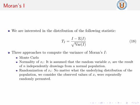
We are interested in the distribution of the following statistic:
TI = I − E(I)√Var(I)
(18)
Three approaches to compute the variance of Moran’s I:Monte CarloNormality of xi: It is assumed that the random variable xi are the resultof n independently drawings from a normal population.Randomization of xi: No matter what the underlying distribution of thepopulation, we consider the observed values of xi were repeatedlyrandomly permuted.

Moran’s I
Theorem (Moran’s I Under Normality)
Assume that {xi} = {x1, x2, ..., xn} are independent and distributed asN(µ, σ2), but µ and σ2 are unknown. Then:
E (I) = − 1n− 1 (19)
and
E(I2) = n2S1 − nS2 + 3S2
0S2
0(n2 − 1) (20)
where S0 =∑n
i=1∑n
j=1 wij, S1 =∑n
i=1∑n
j=1(wij + wji)2/2,S2 =
∑ni=1(wi. + w.i)2, where wi. =
∑nj=1 wij and wi. =
∑nj=1 wji Then:
Var (I) = E(I2)− E (I)2 (21)

Moran’s ITheorem 17 gives the moments of Moran’s I under randomization.
Theorem (Moran’s I Under Randomization)
Under permutation, we have:
E (I) = − 1n− 1 (22)
and
E(I2) =
n[(n2 − 3n+ 3
)S1 − nS2 + 3S2
0]− b2
[(n2 − n
)S1 − 2nS2 + 6S2
0]
(n− 1)(n− 2)(n− 3)S20
(23)where S0 =
∑ni=1∑n
j=1 wij, S1 =∑n
i=1∑n
j=1(wij + wji)2/2,S2 =
∑ni=1(wi. + w.i)2, where wi. =
∑nj=1 wij and wi. =
∑nj=1 wji.Then:
Var (I) = E(I2)− E (I)2 (24)
It is important to note that the expected value of Moran’s I under normalityand randomization is the same.

Monte Carlo
Normality and randomization? We can use a Monte Carlo simulationTo test a null hypothesis H0 we specify a test statistic T such that largevalues of T are evidence against H0.
H0 : no spatial autocorrelation.Let T have observed value tobs. We generally want to calculate:
p = Pr(T ≥ tobs|H0) (25)
We need the distribution of T when H0 is true to evaluate this probability.


Monte Carlo
Theorem (Moran’s’ I Monte Carlo Test)The procedure is the following:
1 Rearrange the spatial data by shuffling their location and compute theMoran’s I S times. This will create the distribution under H0.
2 Let I∗1 , I∗2 , ..., I∗S be the Moran’s I for each time. A consistent Monte Carlop-value is then:
p =1 +
∑Ss=1 1(I∗s ≥ Iobs)S + 1 (26)
3 For tests at the α level or at 100(1− α)% confidence intervals, there arereasons for choosing S so that α(S + 1) is an integer. For example, useS = 999 for confidence intervals and hypothesis tests when α = 0.05.

Inference
Inference:If I > E(I), then a spatial unit tends to be connected by locations withsimilar attributes: Spatial clustering (low/low or high/high). Thestrength of positive spatial autocorrelation tends to increase withI − E(I).If I < E(I) observations will tend to have dissimilar values from theirneighbors: Negative spatial autocorrelation (low/high or high/low)
Application
Lab1A.R
Lab1B.R

Reading for next Class
Dall’Erba, S. (2005). Distribution of regional income and regional fundsin Europe 1989-1999: an exploratory spatial data analysis.The Annals ofRegional Science, 39(1), 121-148.Celebioglu, F., & Dall’erba, S. (2010). Spatial disparities across theregions of Turkey: an exploratory spatial data analysis. The Annals ofRegional Science, 45(2), 379-400.