lec05 new 13 - KTH · valued and G(s) is a matrix (i.e. a matrix-valued function of s). EL2520 Control Theory and Practice Mikael Johansson [email protected] Quiz: transfer matrices

1

EL2520 Control Theory and Practice Mikael Johansson [email protected]

EL2520 Control Theory and Practice

Lecture 5: Multivariable systems

Mikael Johansson School of Electrical Engineering KTH, Stockholm, Sweden


So far…

SISO control revisited: •  Signal norms, system gains and the small gain theorem •  The closed-loop system and the design problem

–  Characterized by six transfer functions: need to look at all! –  Fundamental limitations and waterbed effect.

•  Loop shaping to satisfy sensitivity function specifications.

r

n

u z

w

-F

GFr

wu

y


From now and on: MIMO

Linear systems with multiple inputs and multiple outputs •  Basic properties of multivariable systems •  State-space theory, state feedback and observers •  Decentralized and decoupled control •  Robust loop shaping •  H2 and H1 optimal control

The final part of the course considers systems with constraints


Today’s lecture

Basic properties of multivariable systems •  Transfer matrices •  Block diagram calculations •  Gains and directions •  The multivariable frequency response •  Poles and zeros Chapters 2-3 in the textbook.

2


Transfer matrices

The Laplace transform X(s) of a signal x(t) is defined by Given a linear system and assuming u(t)=0 for t<0 and x(0)=0, If system has multiple inputs and outputs, Y and U are vector- valued and G(s) is a matrix (i.e. a matrix-valued function of s).


Quiz: transfer matrices

1. What is the transfer matrix G(s) for the system How does G(s) change when 2. Input two also affects the first state:

3. The second state also affects output one:

4. The second state influences the first:

Answer and observations

1. Independent subsystems à (block)diagonal transfer matrix 2., 3. Couplings à nondiagonal G(s). Different A, B, C can give same G(s) 4. 1.-4. have the same poles (eigenvalues of A). Hard to see from G(s)


G(s) =

✓ 1s+1 00 1

s+1

◆

G(s) =

✓ 1s+1

1s+1

0 1s+1

◆

G(s) =

✓ 1s+1 � 1

(s+1)2

0 1s+1

◆


Example: series connection

Linear system viewed as interconnected multivariable systems We see that Y(s)=GZ(s)Z(s)= GZ(s)GU(s)U(s). Note that – order matters!

GZGU GUGZ

3


Block diagram calculations

Have to be careful when manipulating block diagrams. Example. Let wu,w,n=0 and derive transfer matrix from r to z so

r

n

u z

w

-F

GFr

wu

y


Quiz: the closed-loop MIMO system

Determine the sensitivity and complementary sensitivity for the linear multivariable system Recall: S is transfer matrix from wàz, T is transfer matrix from -nàz Additional question: What is the relation between S and T?

r

n

u z

w

-F

GFr

wu

y


Today’s lecture

Basic properties of multivariable systems •  Transfer matrices •  Block diagram calculations •  Gains and directions •  The multivariable frequency response •  Poles and zeros


Frequency response and system gain

For a scalar linear system G(s) driven by u(t)=sin(wt), (after transients have died out). So The system gain (cf. Lecture 1) is defined as Attained for sinusoidal input with frequency w such that |G(iw)|=||G||∞ Q: What are the corresponding results for multivariable systems?

4


Operator norm of linear mapping

Consider the linear mapping (x, y, A complex-valued) Since we have So Where are called the singular values of A.


The singular value decomposition A matrix A 2 Cm£ r (with r<m, rank(A)=r), can be represented by its singular value decomposition (SVD) where •  The positive scalars are the singular values of A •  vi are the input singular vectors of A, V*V=I •  ui are the output singular vectors of A, U*U=I

�i


SVD interpretation

Interpretation: linear mapping y=Ax can be decomposed as •  compute coefficients of x along input directions vi •  scale coefficients by •  reconstitute along output directions ui

Since an input in the vr direction is amplified the most. It generates an output in the direction of ur (typically different from vr).

�i

�1 · · · �r


Example

A U ⌃ V

x = v1

5


The multivariable frequency response

For a linear multivariable system Y(s)=G(s)U(s), we have Since this is a linear mapping, with equality if U(iw) parallell w. corresponding input singular vector. For example, only if U(iw) parallell with input singular vector corresponding to


As for scalar systems, we can use Parseval’s theorem to find where Note: Worst-case input is sinusoidal at the frequency that attains the supremum, but its components are appropriately scaled and phase shifted (as specified by the input singular vector of ) Note: the infinity norm computes the maximum amplifications across frequency (sup w) and input directions ( )

The system gain


Example: heat exchanger

Objective: control outlet temperatures Tc, TH by manipulating the flows qC, qH Model:


Singular values of heat exchanger

System gain: ||G||∞=31 dB (=37)

6


Heat exchanger steady-state

Singular value decomposition reveals •  Maximum effect input (input singular vector corresponding to )

•  Minimum effect input (corresponding to )


Heat exchanger step responses

Input direction has dramatic effect! (agrees with physical intuition) Note: large difference in time-scales!


What is the bandwidth of the system? No single value, but a range. Depends on input directions.

Singular values and bandwidths


Today’s lecture

Basic properties of multivariable systems •  Transfer matrices •  Block diagram calculations •  Gains and directions •  The multivariable frequency response •  Poles and zeros

7


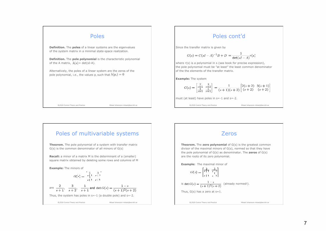
Poles

Definition. The poles of a linear systems are the eigenvalues of the system matrix in a minimal state-space realization. Definition. The pole polynomial is the characteristic polynomial of the A matrix, = det(sI-A). Alternatively, the poles of a linear system are the zeros of the pole polynomial, i.e., the values pi such that

�(s)

�(pi) = 0


Poles cont’d

Since the transfer matrix is given by where r(s) is a polynomial in s (see book for precise expression), the pole polynomial must be ”at least” the least common denominator of the the elements of the transfer matrix. Example: The system must (at least) have poles in s=-1 and s=-2.


Poles of multivariable systems

Theorem. The pole polynomial of a system with transfer matrix G(s) is the common denominator of all minors of G(s) Recall: a minor of a matrix M is the determinant of a (smaller) square matrix obtained by deleting some rows and columns of M Example: The minors of are Thus, the system has poles in s=-1 (a double pole) and s=-2.


Zeros

Theorem. The zero polynomial of G(s) is the greatest common divisor of the maximal minors of G(s), normed so that they have the pole polynomial of G(s) as denominator. The zeros of G(s) are the roots of its zero polynomial. Example: The maximal minor of is (already normed!). Thus, G(s) has a zero at s=1.

8


Notes on poles and zeros For scalar system G(s) with poles pi and zeros zi, For a multivariable system, directions matter! For a system with pole p, there exist vectors up, vp: Similarly, a zero at zi implies the existence of vectors uz, vz: As for scalar systems, a zero at s=z implies that there exists a signal on the form u(t)=vze-zt for t¸ 0, and u(t)=0 for t<0, and initial values x(0)=xz so that y(t)=0 for t¸ 0

Zeroes and directions

Example. Although none of the elements of has a zero, the system has a non-minimum phase zero for s=1. By the SVD we find uz and vz as the second columns of U and V, respectively.


G(1) =

�0.894 �0.4472�0.4472 0.8944

� 1.5811 0

0 0

� �0.7071 �0.7071�0.7071 0.7071

�⇤

uTz G(s)vz =

�0.44720.8944

�T 2s+1

3s+2

1s+1

1s+1

� �0.70710.7071

�⇤= 0.3162

(1� s)

s2 + 3s+ 2

Zeroes and directions

Example cont’d. Simulating the system with input (-1,1) yields A clear non-minimum phase effect!


0 1 2 3 4 5 6 7 8 9 10−0.6

−0.4

−0.2

0

0.2

Time

Oup

uts

1 an

d 2


Summary

An introduction to multivariable linear systems: •  Block diagram manipulations (order matters!) •  System gain (directions matter!) •  Poles and zeros

More next week!

Documents

lec05 new 13 - KTH · valued and G(s) is a matrix (i.e. a matrix-valued function of s). EL2520 Control Theory and Practice Mikael Johansson [email protected] Quiz: transfer matrices