Learning with general recurrent neural networks

Guy Isely

Feedforward neural networks are “timeless”

664 Chapter 40

Output Units

/ k / CCOXO

Processing Unit

b

Total Input E

Figure 1 (a) Schematic model of a processing unit receiving inputs from other processing units. (b) Transformation between summed inputs and output of a processing unit, as given by Eq. 2.

speech. The model, which we call NETtalk, demon- strates that a relatively small network can capture most of the significant regularities in English pronunciation as well as absorb many of the irregularities. NETtalk can be trained on any dialect of any language and the resulting network can be implemented directly in hardware.

We will first describe the network architecture and the learning algorithm that we used, and then present the results obtained from simulations. Finally, we dis- cuss the computational complexity of NETtalk and some of its biological implications.

Network ~rchitecture

Processing Units The network is composed of processing units that non- linearly transform their summed, continuous-valued inputs, as illustrated in Fig. 1. The connection strength, or weight, linking one unit to another unit can be a positive or negative real value, representing either an excitatory or an inhibitory influence of the first unit on the output of the second unit. Each unit also has a threshold which is subtracted from the summed input. The threshold is implemented as weight from a unit that has a fixed value of 1 so that the same notation and learning algorithm can also be applied to the thresholds as well as the weights. The output of the ith unit is determined by first summing all of its inputs

E i = 1 WijP j j

(1)

where wij is the weight from the jth to the ith unit, and then applying a sigmoidal transformation

H ~ d d e n Units

Input Uni ts

Figure 2 Schematic drawing of the network architecture. Input units are shown on the bottom of the pyramid, with 7 groups of 29 units in each group. Each hidden unit in the intermediate layer receives inputs from all of the input units on the bottom layer, and in turn sends its output to all 26 units in the output layer. An example of an input string of letters is shown below the inputs groups, and the correct output phoneme for the middle letter is shown above the output layer. For 80 hidden units, which were used for the corpus of continuous informal speech, there was a total of 309 units and 18,629 weights in the network, including a variable threshold for each unit.

as shown in Fig. 1. The network used in NETtalk is hierarchically

arranged into three layers of units: an input layer, an output layer and an intermediate or "hidden" layer, as illustrated in Fig. 2. Information flows through the network from bottom to top. First the letters units at the base are clamped, then the states of the hidden units are determined by Eqs. 1 & 2, and finally, the states of the phoneme units at the top are determined (30).

Representations of Letters and Phonemes There are seven groups of units in the input layer, and one group of units in each of the other two layers. Each input group encodes one letter of the input text, so that strings of seven letters are presented to the input units at any one time. The desired output of the network is the correct phoneme, or contrastive speech sound, associated with the center, or fourth, letter of this seven letter "window". The other six letters (three on either side of the center letter) provide a partial context for this decision. The test is stepped through the window letter-by-letter. At each step, the network computes a phoneme, and after each word the weights are adjusted according to how closely the computed ~ronunciation matches the correct one.

The letters and phonemes are represented in differ- ent ways. The letters are represented locally within

t?

Some problems with a feedforward model of temporal processes

• Computational cost grows with temporal duration modeled

• Can’t capture long-time contextual dependencies in sequences

• Networks don’t have persistent state— “noise correlations” might be state!

Hopfield networks have fixed-point attractor dynamics

• Dynamics are gradient descent on an energy function (the lyapunov function)

• Autonomous after initial input

• Guaranteed to converge to a stable fixed point due to symmetric connectivity matrix

Can we you use gradient descent to train general RNNs?

Yes, yes we can!

…but there’s a wrinkle.

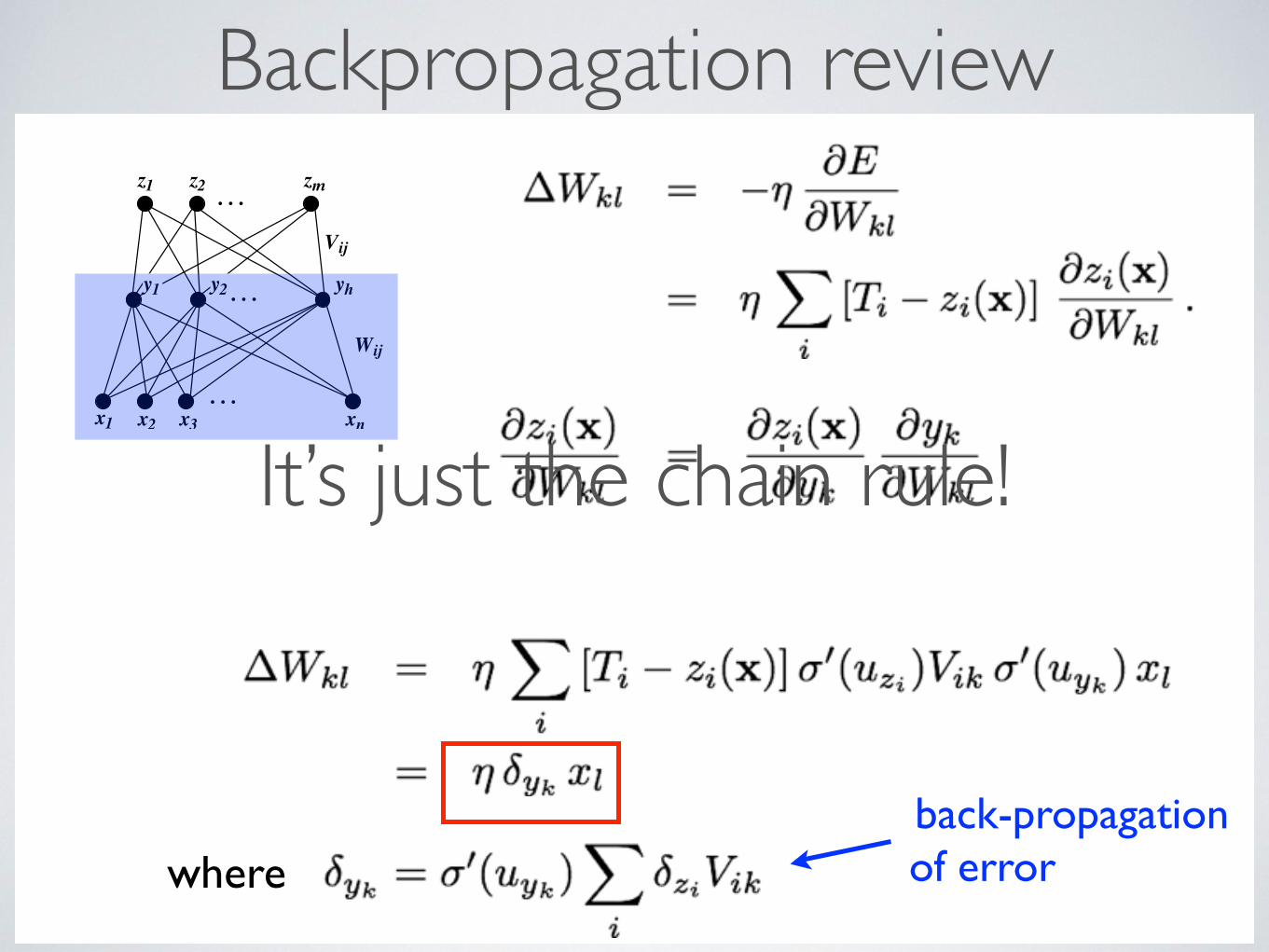
Backpropagation reviewLearning rule for hidden layer

. . .x1 x2 x3 xn

. . .

Wij

. . .

y1 y2 yh

Vij

z1 z2 zmoutput

"hidden units"

input

whereback-propagation!of error

It’s just the chain rule!

Can we apply backpropagation directly to an RNN?

• Not exactly— the gradient of a RNN’s error function w.r.t. to the weights depends on the network’s state at all previous time steps.

• But we can unravel the network structure in time to get a feedforward network and perform backprop on this network.

• This is called backpropagation through time (BPTT).

Realtime recurrent learning (Williams and Zipser 1989)

•

• We can run the recurrence relation underlying the gradient computation forward in time!

• Downside: BPTT is O(tn2) per time step but RTRL is O(n3) per time step— prohibitive for large networks!

@y(t)

@Wr= diag(�0(y(t)))W> · @y(t� 1)

@Wr

Intermission (aka neural network winter)

Reservoir computing

Harnessing Nonlinearity: PredictingChaotic Systems and Saving Energyin Wireless Communication

Herbert Jaeger* and Harald Haas

We present a method for learning nonlinear systems, echo state networks(ESNs). ESNs employ artificial recurrent neural networks in a way that hasrecently been proposed independently as a learning mechanism in biologicalbrains. The learning method is computationally efficient and easy to use. Ona benchmark task of predicting a chaotic time series, accuracy is improved bya factor of 2400 over previous techniques. The potential for engineering ap-plications is illustrated by equalizing a communication channel, where the signalerror rate is improved by two orders of magnitude.

Nonlinear dynamical systems abound in thesciences and in engineering. If one wishes tosimulate, predict, filter, classify, or control sucha system, one needs an executable system mod-el. However, it is often infeasible to obtainanalytical models. In such cases, one has toresort to black-box models, which ignore theinternal physical mechanisms and instead re-produce only the outwardly observable input-output behavior of the target system.

If the target system is linear, efficientmethods for black-box modeling are avail-able. Most technical systems, however, be-come nonlinear if operated at higher opera-tional points (that is, closer to saturation).Although this might lead to cheaper and moreenergy-efficient designs, it is not done be-cause the resulting nonlinearities cannot beharnessed. Many biomechanical systems usetheir full dynamic range (up to saturation)and thereby become lightweight, energy effi-cient, and thoroughly nonlinear.

Here, we present an approach to learn-ing black-box models of nonlinear systems,echo state networks (ESNs). An ESN is anartificial recurrent neural network (RNN).RNNs are characterized by feedback (“re-current”) loops in their synaptic connectionpathways. They can maintain an ongoingactivation even in the absence of input andthus exhibit dynamic memory. Biologicalneural networks are typically recurrent.Like biological neural networks, an artifi-cial RNN can learn to mimic a targetsystem—in principle, with arbitrary accu-racy (1). Several learning algorithms areknown (2!4) that incrementally adapt thesynaptic weights of an RNN in order totune it toward the target system. Thesealgorithms have not been widely employedin technical applications because of slow

convergence and suboptimal solutions (5,6). The ESN approach differs from thesemethods in that a large RNN is used (on theorder of 50 to 1000 neurons; previous tech-niques typically use 5 to 30 neurons) and inthat only the synaptic connections from theRNN to the output readout neurons aremodified by learning; previous techniquestune all synaptic connections (Fig. 1). Be-cause there are no cyclic dependencies be-tween the trained readout connections,training an ESN becomes a simple linearregression task.

We illustrate the ESN approach on atask of chaotic time series prediction (Fig.2) (7). The Mackey-Glass system (MGS)(8) is a standard benchmark system for timeseries prediction studies. It generates a sub-tly irregular time series (Fig. 2A). Theprediction task has two steps: (i) using aninitial teacher sequence generated by theoriginal MGS to learn a black-box model Mof the generating system, and (ii) using Mto predict the value of the sequence somesteps ahead.

First, we created a random RNN with1000 neurons (called the “reservoir”) and oneoutput neuron. The output neuron wasequipped with random connections thatproject back into the reservoir (Fig. 2B). A3000-step teacher sequence d(1), . . .,d(3000) was generated from the MGS equa-tion and fed into the output neuron. Thisexcited the internal neurons through the out-put feedback connections. After an initialtransient period, they started to exhibit sys-tematic individual variations of the teachersequence (Fig. 2B).

The fact that the internal neurons displaysystematic variants of the exciting externalsignal is constitutional for ESNs: The internalneurons must work as “echo functions” forthe driving signal. Not every randomly gen-erated RNN has this property, but it caneffectively be built into a reservoir (support-ing online text).

It is important that the echo signals berichly varied. This was ensured by a sparseinterconnectivity of 1% within the reservoir.This condition lets the reservoir decomposeinto many loosely coupled subsystems, estab-lishing a richly structured reservoir of excit-able dynamics.

After time n " 3000, output connectionweights wi (i " 1, . . . , 1000) were computed(dashed arrows in Fig. 2B) from the last 2000steps n " 1001, . . . , 3000 of the training runsuch that the training error

MSEtrain"1/2000!n"1001

3000 "d(n)!!i ! 1

1000

w i xi(n)#2

was minimized [xi(n), activation of the ithinternal neuron at time n]. This is a simplelinear regression.

With the new wi in place, the ESN wasdisconnected from the teacher after step 3000and left running freely. A bidirectional dy-namical interplay of the network-generatedoutput signal with the internal signals xi(n)unfolded. The output signal y(n) was createdfrom the internal neuron activation signalsxi(n) through the trained connections wi, by

y(n)"#i"1

1000wixi$n). Conversely, the internal

signals were echoed from that output signalthrough the fixed output feedback connec-tions (supporting online text).

For testing, an 84-step continuationd(3001), . . . , d(3084) of the original signalwas computed for reference. The networkoutput y(3084) was compared with the cor-rect continuation d(3084). Averaged over 100independent trials, a normalized root meansquare error

NRMSE " "!j"1

100

(dj(3084) ! yj$3084))2/100%2&#1/2

'10!4.2

was obtained (dj and yj teacher and network

International University Bremen, Bremen D-28759,Germany.

*To whom correspondence should be addressed. E-mail: h.jaeger@iu-bremen.de

Fig. 1. (A) Schema of previous approaches toRNN learning. (B) Schema of ESN approach.Solid bold arrows, fixed synaptic connections;dotted arrows, adjustable connections. Bothapproaches aim at minimizing the error d(n) –y(n), where y(n) is the network output and d(n)is the teacher time series observed from thetarget system.

R E P O R T S

2 APRIL 2004 VOL 304 SCIENCE www.sciencemag.org78

on

Mar

ch 8

, 201

3w

ww

.sci

ence

mag

.org

Dow

nloa

ded

from

Echo State Networks (Jaeger & Haas 2004) 2540 Wolfgang Maass, Thomas Natschlager, and Henry Markram

0

20

40

input�pattern�"one"

0

45

90

135

liquid�response

0

25

50

readout�response

0

1

correctness

0 0.1 0.2 0.3 0.4 0.5

0

1

certainty

time�[s]

0

45

90

135

liquid�response

ne

uron

�#

0

25

50

readout�response

ne

uron�#

0

1

correctness

0 0.1 0.2 0.3 0.4 0.5

0

1

certainty

time�[s]

0

20

40

input�pattern�"zero"

neu

ro

n�#

6 Exploring the Computational Power of Models for NeuralMicrocircuit

As a érst test of its computational power, this simple generic circuit was ap-plied to a previously considered classiécation task (Hopéeld & Brody, 2001),where spoken words were represented by noise-corrupted spatiotemporalspike patterns over a rather long time interval (40-channel spike patternsover 0.5 sec). This classiécation task had been solved in Hopéeld and Brody(2001) by a network of neurons designed for this task (relying on unknown

Liquid State Machines (Maass et al. 2002)

Ideas from Echo State Networks

• Use an unoptimized random sparsely connected recurrent reservoir and do a linear readout.

• Only optimize the readout weights.

• Use teacher forcing to achieve appropriately tuned the reservoir dynamics

BPTT returns (with a vengeance)

Where to next?• Address vanishing/exploding sensitivity problem with network

units designed for specific temporal dynamics (e.g. Long Short Term Memory)

• Move beyond gradient descent based approaches to optimizing network parameters

• Incorporate addition biophysical features of real networks (e.g. STDP, metabotropic receptor dynamics, gap junctions, dendritic non-linearities)