Embed Size (px)
Citation preview

Learning with Big Data I: Divide and Conquer
lti
lti ablc
28 July 2014 – LxMLS
Chris Dyer
No data like more data!
(Banko and Brill, ACL 2001) (Brants et al., EMNLP 2007)
Training Instances
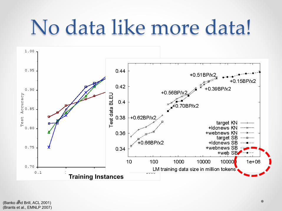
Problem
#(t) ~ n0 × 2t/(2 years)~Moore’s law (~ power/CPU)
#(t) ~ m0 × 3.2t/(2 years)~Hard disk capacity
We can represent more data than we can centrally process ... and this will
only get worse in the future.

Solution • Partition training data into subsets
o Core concept: data shards o Algorithms that work primarily “inside” shards and communicate minimally o Nodes is a graph, edges represent communication pathways
• Alternative solutions o Reduce data points by instance selection (e.g. core sets) o Dimensionality reduction / compression
• Related problems o Large numbers of dimensions (horizontal partitioning)
• Model is too big to fit in memory o Large numbers of related tasks
• every Gmail user has his own opinion about what is spam
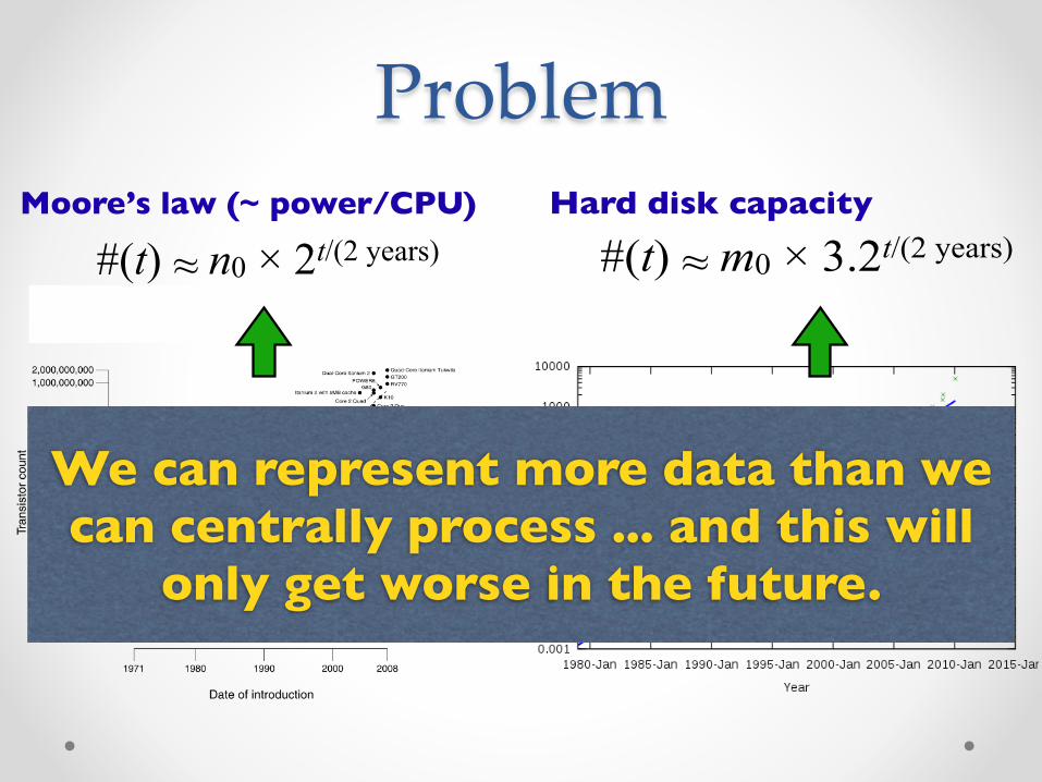
Outline • MapReduce • Design patterns for MapReduce
• Batch Learning Algorithms on MapReduce • Distributed Online Algorithms
+ simple, distributed programming models cheap commodity clusters
= data-intensive computing for all
MapReduce

Divide and Conquer “Work”
w1 w2 w3
r1 r2 r3
“Result”
“worker”
“worker”
“worker”
Partition
Combine
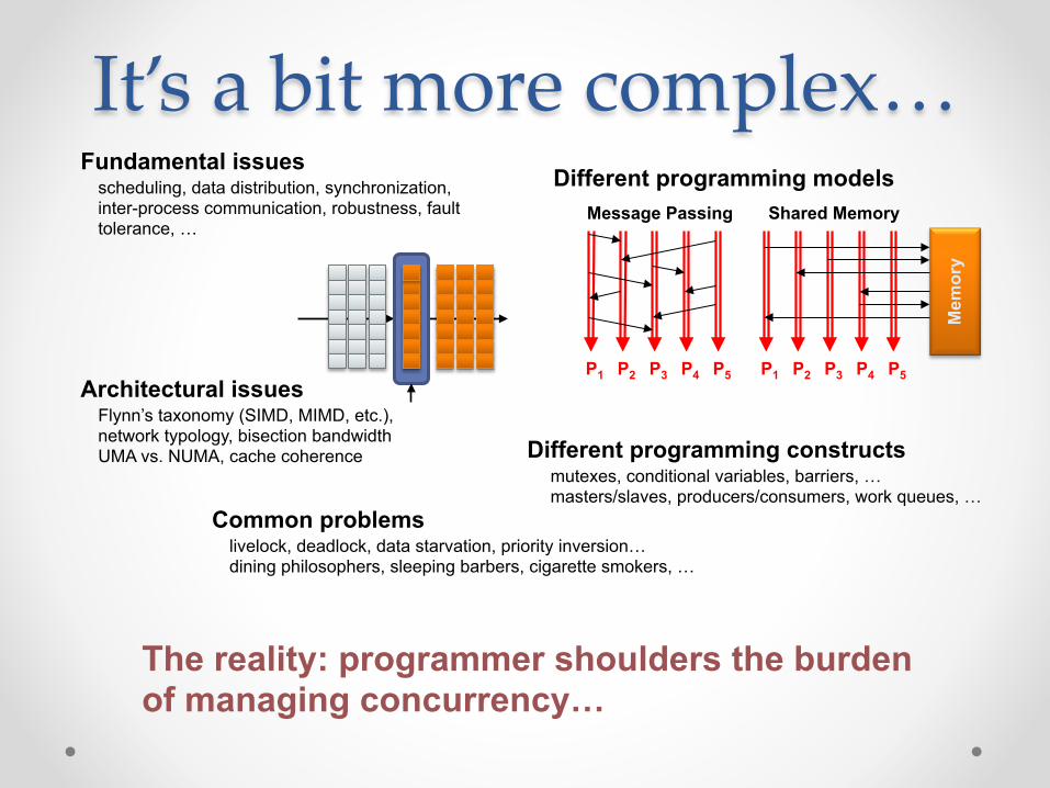
It’s a bit more complex… Message Passing
P1 P2 P3 P4 P5
Shared Memory
P1 P2 P3 P4 P5
Mem
ory
Different programming models
Different programming constructs mutexes, conditional variables, barriers, … masters/slaves, producers/consumers, work queues, …
Fundamental issues scheduling, data distribution, synchronization, inter-process communication, robustness, fault tolerance, …
Common problems livelock, deadlock, data starvation, priority inversion… dining philosophers, sleeping barbers, cigarette smokers, …
Architectural issues Flynn’s taxonomy (SIMD, MIMD, etc.), network typology, bisection bandwidth UMA vs. NUMA, cache coherence
The reality: programmer shoulders the burden of managing concurrency…

Source: Ricardo Guimarães Herrmann
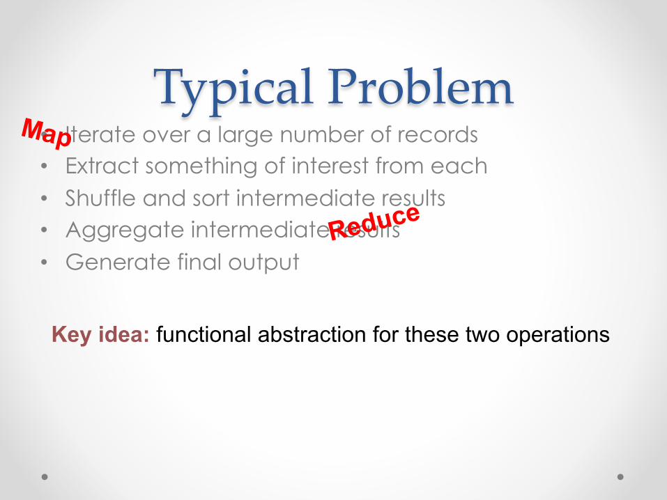
Typical Problem • Iterate over a large number of records • Extract something of interest from each • Shuffle and sort intermediate results • Aggregate intermediate results • Generate final output
Key idea: functional abstraction for these two operations
Map
Reduce

g g g g g
f f f f f Map
Fold
Map
Reduce
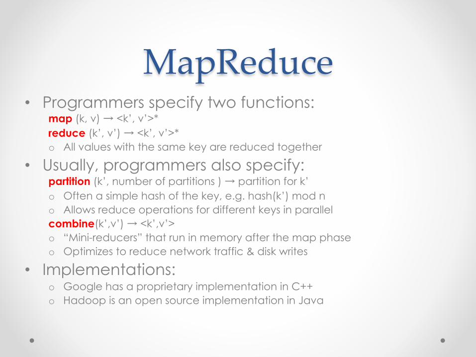
MapReduce • Programmers specify two functions:
map (k, v) → <k’, v’>* reduce (k’, v’) → <k’, v’>* o All values with the same key are reduced together
• Usually, programmers also specify: partition (k’, number of partitions ) → partition for k’ o Often a simple hash of the key, e.g. hash(k’) mod n o Allows reduce operations for different keys in parallel combine(k’,v’) → <k’,v’> o “Mini-reducers” that run in memory after the map phase o Optimizes to reduce network traffic & disk writes
• Implementations: o Google has a proprietary implementation in C++ o Hadoop is an open source implementation in Java

map map map map
Shuffle and Sort: aggregate values by keys
reduce reduce reduce
k1 k2 k3 k4 k5 k6 v1 v2 v3 v4 v5 v6
b a 1 2 c c 3 6 a c 5 2 b c 7 9
a 1 5 b 2 7 c 2 3 6 9
r1 s1 r2 s2 r3 s3
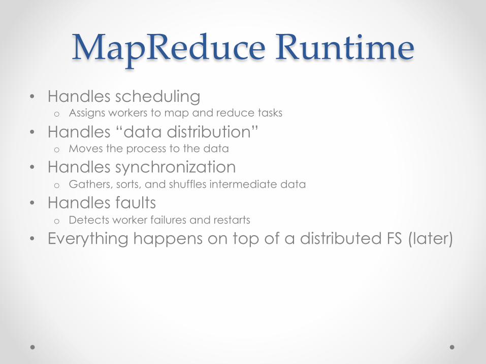
MapReduce Runtime • Handles scheduling
o Assigns workers to map and reduce tasks
• Handles “data distribution” o Moves the process to the data
• Handles synchronization o Gathers, sorts, and shuffles intermediate data
• Handles faults o Detects worker failures and restarts
• Everything happens on top of a distributed FS (later)

“Hello World”: Word Count
Map(String input_key, String input_value): // input_key: document name // input_value: document contents for each word w in input_values: EmitIntermediate(w, "1"); Reduce(String key, Iterator intermediate_values): // key: a word, same for input and output // intermediate_values: a list of counts int result = 0; for each v in intermediate_values: result += ParseInt(v); Emit(AsString(result));

split 0 split 1 split 2 split 3 split 4
worker
worker
worker
worker
worker
Master
User Program
output file 0
output file 1
(1) fork (1) fork (1) fork
(2) assign map (2) assign reduce
(3) read (4) local write
(5) remote read (6) write
Input files
Map phase
Intermediate files (on local disk)
Reduce phase
Output files
Redrawn from Dean and Ghemawat (OSDI 2004)
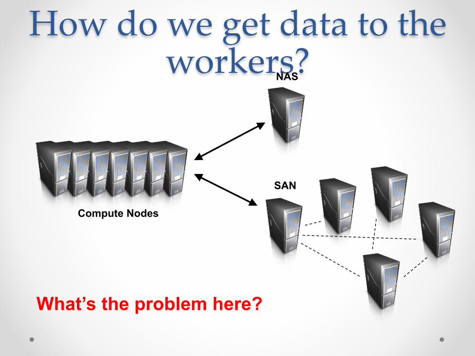
How do we get data to the workers?
Compute Nodes
NAS
SAN
What’s the problem here?

Distributed File System • Don’t move data to workers… Move workers to the
data! o Store data on the local disks for nodes in the cluster o Start up the workers on the node that has the data local
• Why? o Not enough RAM to hold all the data in memory o Disk access is slow, disk throughput is good
• A distributed file system is the answer o GFS (Google File System) o HDFS for Hadoop (= GFS clone)
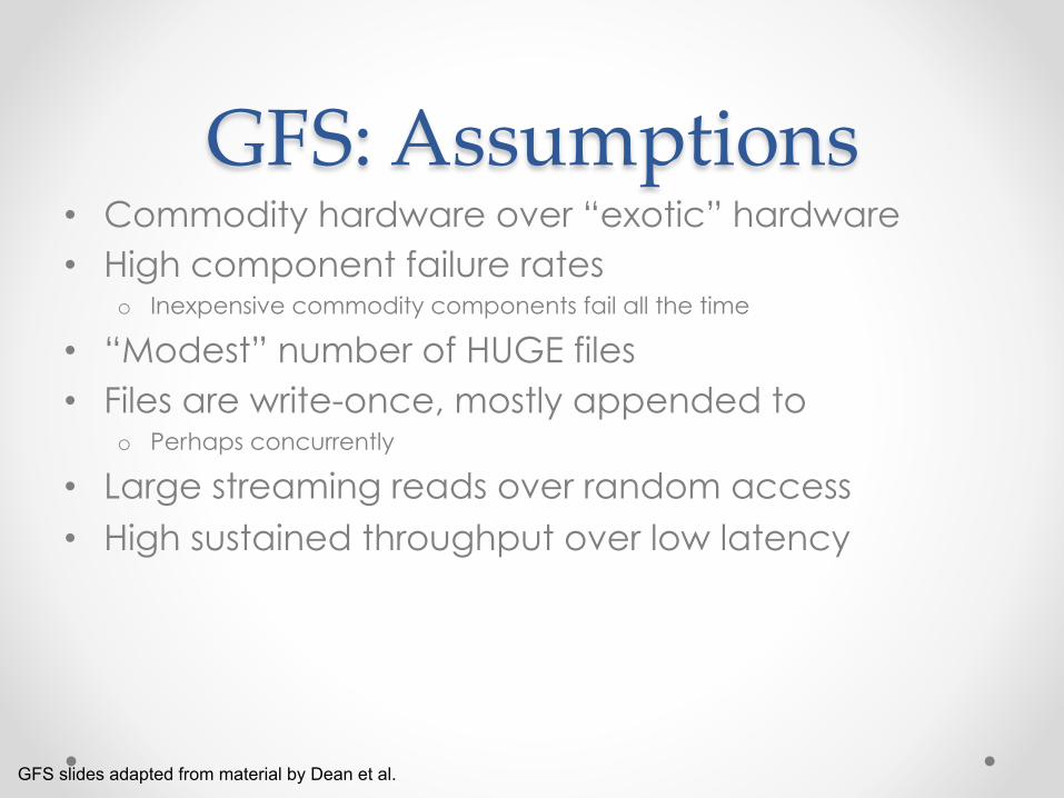
GFS: Assumptions • Commodity hardware over “exotic” hardware • High component failure rates
o Inexpensive commodity components fail all the time
• “Modest” number of HUGE files • Files are write-once, mostly appended to
o Perhaps concurrently
• Large streaming reads over random access • High sustained throughput over low latency
GFS slides adapted from material by Dean et al.
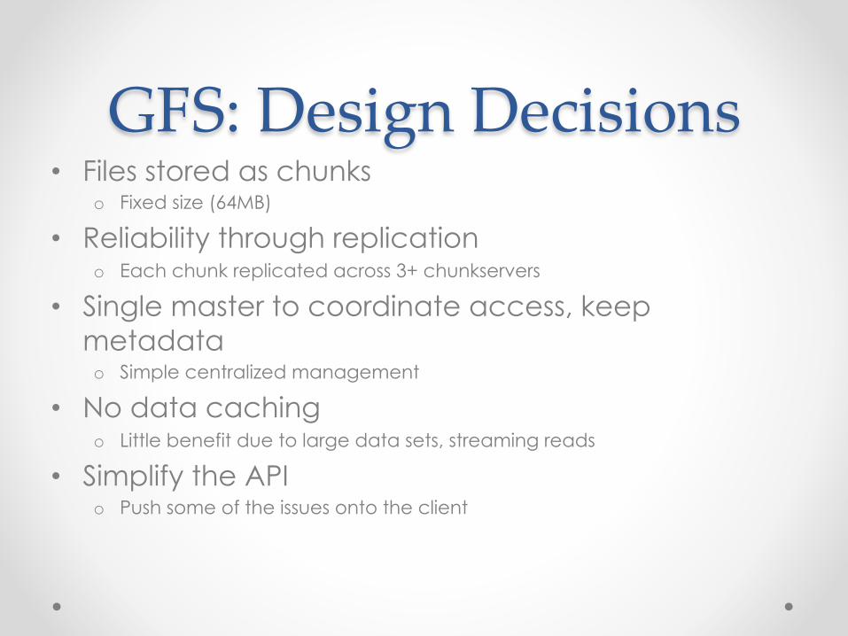
GFS: Design Decisions • Files stored as chunks
o Fixed size (64MB)
• Reliability through replication o Each chunk replicated across 3+ chunkservers
• Single master to coordinate access, keep metadata o Simple centralized management
• No data caching o Little benefit due to large data sets, streaming reads
• Simplify the API o Push some of the issues onto the client
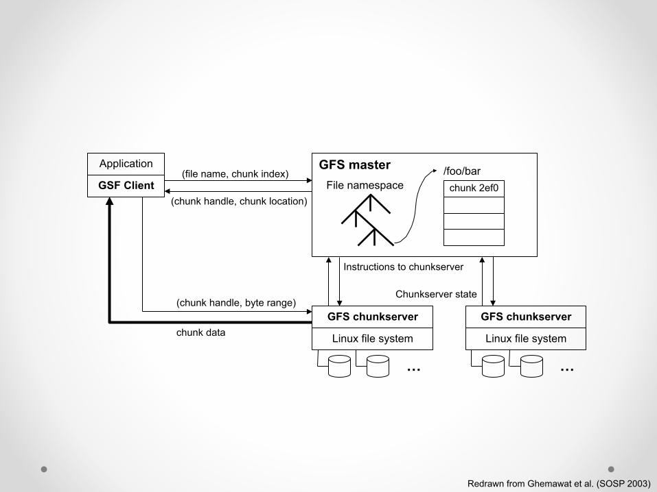
Redrawn from Ghemawat et al. (SOSP 2003)
Application
GSF Client
GFS master File namespace
/foo/bar chunk 2ef0
GFS chunkserver
Linux file system
…
GFS chunkserver
Linux file system
…
(file name, chunk index)
(chunk handle, chunk location)
Instructions to chunkserver
Chunkserver state (chunk handle, byte range)
chunk data

Master’s Responsibilities • Metadata storage • Namespace management/locking • Periodic communication with chunkservers • Chunk creation, replication, rebalancing • Garbage collection

Questions?
MapReduce “killer app”: Graph Algorithms

Graph Algorithms: Topics • Introduction to graph algorithms and graph
representations • Single Source Shortest Path (SSSP) problem
o Refresher: Dijkstra’s algorithm o Breadth-First Search with MapReduce
• PageRank
What’s a graph? • G = (V,E), where
o V represents the set of vertices (nodes) o E represents the set of edges (links) o Both vertices and edges may contain additional information
• Different types of graphs: o Directed vs. undirected edges o Presence or absence of cycles o …
Some Graph Problems • Finding shortest paths
o Routing Internet traffic and UPS trucks
• Finding minimum spanning trees o Telco laying down fiber
• Finding Max Flow o Airline scheduling
• Identify “special” nodes and communities o Breaking up terrorist cells, spread of swine/avian/… flu
• Bipartite matching o Monster.com, Match.com
• And of course... PageRank
Representing Graphs • G = (V, E)
o A poor representation for computational purposes
• Two common representations o Adjacency matrix o Adjacency list
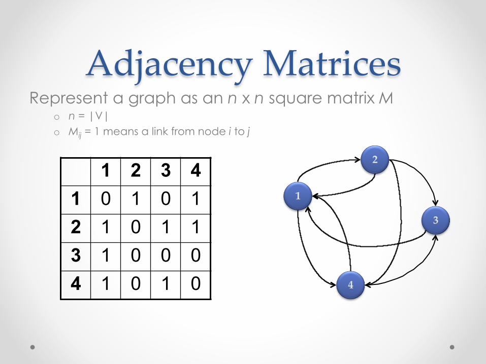
Adjacency Matrices Represent a graph as an n x n square matrix M
o n = |V| o Mij = 1 means a link from node i to j
1 2 3 4 1 0 1 0 1 2 1 0 1 1 3 1 0 0 0 4 1 0 1 0
1
2
3
4

Adjacency Lists Take adjacency matrices… and throw away all the
zeros
1 2 3 4 1 0 1 0 1 2 1 0 1 1 3 1 0 0 0 4 1 0 1 0
1: 2, 4 2: 1, 3, 4 3: 1 4: 1, 3
Adjacency Lists: Critique • Advantages:
o Much more compact representation o Easy to compute over outlinks o Graph structure can be broken up and distributed
• Disadvantages: o Much more difficult to compute over inlinks
Single Source Shortest Path
• Problem: find shortest path from a source node to one or more target nodes
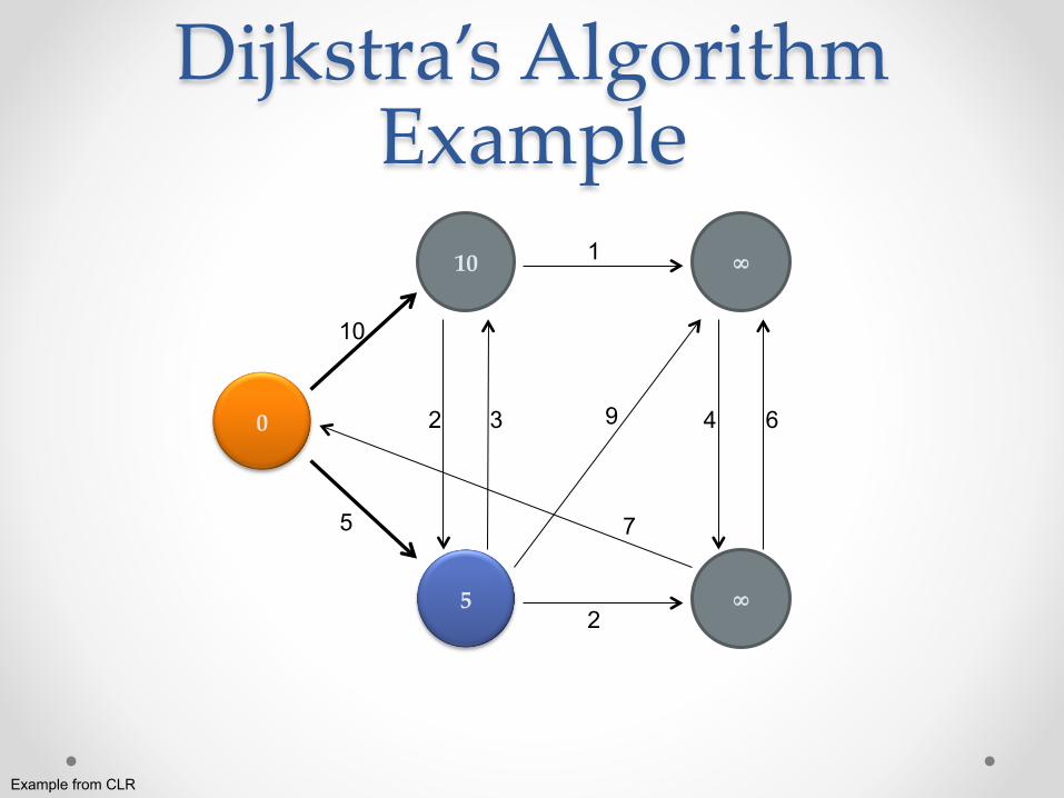
• First, a refresher: Dijkstra’s Algorithm

Dijkstra’s Algorithm Example
0
∞
∞
∞
∞
10
5
2 3
2
1
9
7
4 6
Example from CLR
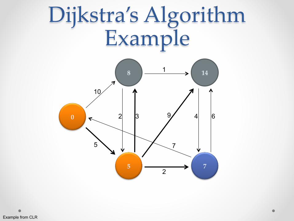
Dijkstra’s Algorithm Example
0
10
5
∞
∞
10
5
2 3
2
1
9
7
4 6
Example from CLR
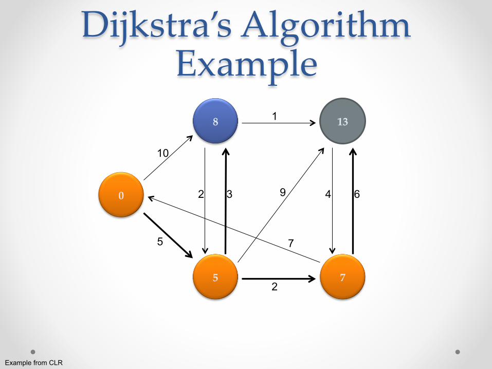
Dijkstra’s Algorithm Example
0
8
5
14
7
10
5
2 3
2
1
9
7
4 6
Example from CLR
Dijkstra’s Algorithm Example
0
8
5
13
7
10
5
2 3
2
1
9
7
4 6
Example from CLR

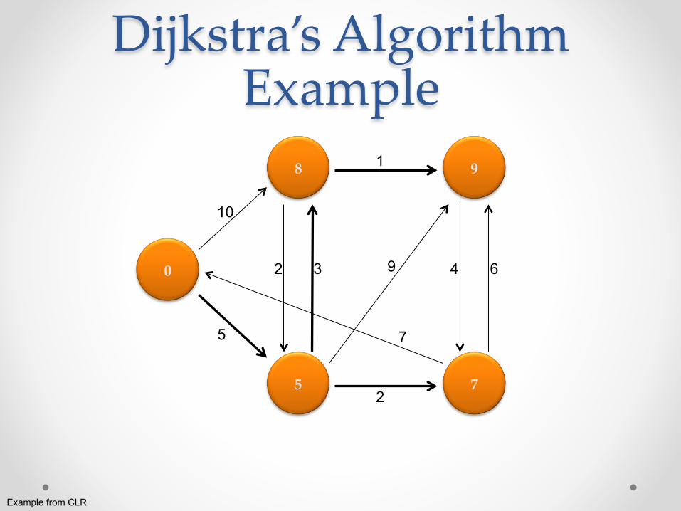
Dijkstra’s Algorithm Example
0
8
5
9
7
10
5
2 3
2
1
9
7
4 6
Example from CLR
Dijkstra’s Algorithm Example
0
8
5
9
7
10
5
2 3
2
1
9
7
4 6
Example from CLR
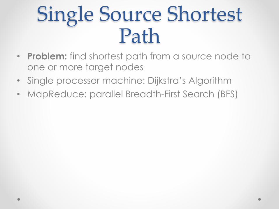
Single Source Shortest Path
• Problem: find shortest path from a source node to one or more target nodes
• Single processor machine: Dijkstra’s Algorithm • MapReduce: parallel Breadth-First Search (BFS)

Finding the Shortest Path • First, consider equal edge weights • Solution to the problem can be defined inductively • Here’s the intuition:
o DistanceTo(startNode) = 0 o For all nodes n directly reachable from startNode,
DistanceTo(n) = 1
o For all nodes n reachable from some other set of nodes S, DistanceTo(n) = 1 + min(DistanceTo(m), m ∈ S)

From Intuition to Algorithm
• A map task receives o Key: node n o Value: D (distance from start), points-to (list of nodes reachable from n)
• ∀p ∈ points-to: emit (p, D+1) • The reduce task gathers possible distances to a
given p and selects the minimum one

Multiple Iterations Needed
• This MapReduce task advances the “known frontier” by one hop o Subsequent iterations include more reachable nodes as frontier advances o Multiple iterations are needed to explore entire graph o Feed output back into the same MapReduce task
• Preserving graph structure: o Problem: Where did the points-to list go? o Solution: Mapper emits (n, points-to) as well

Visualizing Parallel BFS 1
2 2
2 3
3
3 3
4
4
Termination • Does the algorithm ever terminate?
o Eventually, all nodes will be discovered, all edges will be considered (in a connected graph)
• When do we stop?

Weighted Edges • Now add positive weights to the edges • Simple change: points-to list in map task includes a
weight w for each pointed-to node o emit (p, D+wp) instead of (p, D+1) for each node p
• Does this ever terminate? o Yes! Eventually, no better distances will be found. When distance is the
same, we stop o Mapper should emit (n, D) to ensure that “current distance” is carried into
the reducer

Comparison to Dijkstra • Dijkstra’s algorithm is more efficient
o At any step it only pursues edges from the minimum-cost path inside the frontier
• MapReduce explores all paths in parallel o Divide and conquer o Throw more hardware at the problem
General Approach • MapReduce is adept at manipulating graphs
o Store graphs as adjacency lists
• Graph algorithms with for MapReduce: o Each map task receives a node and its outlinks o Map task compute some function of the link structure, emits value with
target as the key o Reduce task collects keys (target nodes) and aggregates
• Iterate multiple MapReduce cycles until some termination condition o Remember to “pass” graph structure from one iteration to next

Random Walks Over the Web
• Model: o User starts at a random Web page o User randomly clicks on links, surfing from page to page
• PageRank = the amount of time that will be spent on any given page
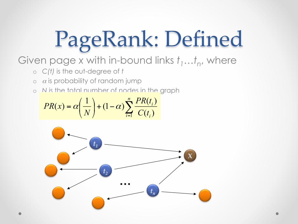
PageRank: Defined Given page x with in-bound links t1…tn, where
o C(t) is the out-degree of t o α is probability of random jump o N is the total number of nodes in the graph
∑=
−+⎟⎠
⎞⎜⎝
⎛=n
i i
i
tCtPR
NxPR
1 )()()1(1)( αα
X
t1
t2
tn …

Computing PageRank • Properties of PageRank
o Can be computed iteratively o Effects at each iteration is local
• Sketch of algorithm: o Start with seed PRi values o Each page distributes PRi “credit” to all pages it links to o Each target page adds up “credit” from multiple in-bound links to
compute PRi+1
o Iterate until values converge

PageRank in MapReduce Map: distribute PageRank “credit” to link targets
...
Reduce: gather up PageRank “credit” from multiple sources to compute new PageRank value
Iterate until convergence

PageRank: Issues • Is PageRank guaranteed to converge? How
quickly? • What is the “correct” value of α, and how sensitive is
the algorithm to it? • What about dangling links? • How do you know when to stop?

Graph algorithms in MapReduce
• General approach o Store graphs as adjacency lists (node, points-to, points-to …) o Mappers receive (node, points-to*) tuples o Map task computes some function of the link structure o Output key is usually the target node in the adjacency list representation o Mapper typically outputs the graph structure as well
• Iterate multiple MapReduce cycles until some convergence criterion is met

Questions?

MapReduce Algorithm Design

Managing Dependencies • Remember: Mappers run in isolation
o You have no idea in what order the mappers run o You have no idea on what node the mappers run o You have no idea when each mapper finishes
• Tools for synchronization: o Ability to hold state in reducer across multiple key-value pairs o Sorting function for keys o Partitioner o Cleverly-constructed data structures

Motivating Example • Term co-occurrence matrix for a text collection
o M = N x N matrix (N = vocabulary size) o Mij: number of times i and j co-occur in some context
(for concreteness, let’s say context = sentence)
• Why? o Distributional profiles as a way of measuring semantic distance o Semantic distance useful for many language processing tasks
“You shall know a word by the company it keeps” (Firth, 1957)
e.g., Mohammad and Hirst (EMNLP, 2006)

MapReduce: Large Counting Problems
• Term co-occurrence matrix for a text collection = specific instance of a large counting problem o A large event space (number of terms) o A large number of events (the collection itself) o Goal: keep track of interesting statistics about the events
• Basic approach o Mappers generate partial counts o Reducers aggregate partial counts
How do we aggregate partial counts efficiently?
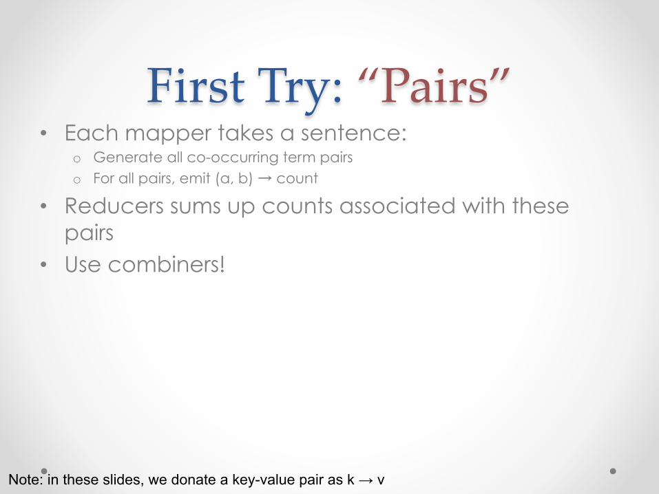
First Try: “Pairs” • Each mapper takes a sentence:
o Generate all co-occurring term pairs o For all pairs, emit (a, b) → count
• Reducers sums up counts associated with these pairs
• Use combiners!
Note: in these slides, we donate a key-value pair as k → v

“Pairs” Analysis • Advantages
o Easy to implement, easy to understand
• Disadvantages o Lots of pairs to sort and shuffle around (upper bound?)
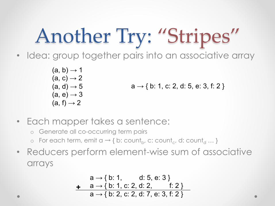
Another Try: “Stripes” • Idea: group together pairs into an associative array
• Each mapper takes a sentence: o Generate all co-occurring term pairs o For each term, emit a → { b: countb, c: countc, d: countd … }
• Reducers perform element-wise sum of associative arrays
(a, b) → 1 (a, c) → 2 (a, d) → 5 (a, e) → 3 (a, f) → 2
a → { b: 1, c: 2, d: 5, e: 3, f: 2 }
a → { b: 1, d: 5, e: 3 } a → { b: 1, c: 2, d: 2, f: 2 } a → { b: 2, c: 2, d: 7, e: 3, f: 2 }
+

“Stripes” Analysis • Advantages
o Far less sorting and shuffling of key-value pairs o Can make better use of combiners
• Disadvantages o More difficult to implement o Underlying object is more heavyweight o Fundamental limitation in terms of size of event space

Cluster size: 38 cores Data Source: Associated Press Worldstream (APW) of the English Gigaword Corpus (v3), which contains 2.27 million documents (1.8 GB compressed, 5.7 GB uncompressed)

Relative frequency estimates
• How do we compute relative frequencies from counts?
• Why do we want to do this? • How do we do this with MapReduce?
∑==
')',(count),(count
)(count),(count)|(
BBABA
ABAABP
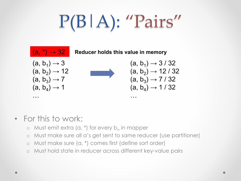
P(B|A): “Pairs”
• For this to work: o Must emit extra (a, *) for every bn in mapper o Must make sure all a’s get sent to same reducer (use partitioner) o Must make sure (a, *) comes first (define sort order) o Must hold state in reducer across different key-value pairs
(a, b1) → 3 (a, b2) → 12 (a, b3) → 7 (a, b4) → 1 …
(a, *) → 32
(a, b1) → 3 / 32 (a, b2) → 12 / 32 (a, b3) → 7 / 32 (a, b4) → 1 / 32 …
Reducer holds this value in memory

P(B|A): “Stripes”
• Easy! o One pass to compute (a, *) o Another pass to directly compute f(B|A)
a → {b1:3, b2 :12, b3 :7, b4 :1, … }
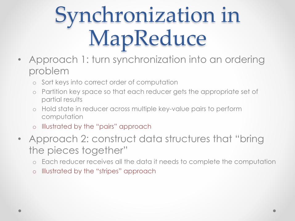
Synchronization in MapReduce
• Approach 1: turn synchronization into an ordering problem o Sort keys into correct order of computation o Partition key space so that each reducer gets the appropriate set of
partial results o Hold state in reducer across multiple key-value pairs to perform
computation
o Illustrated by the “pairs” approach
• Approach 2: construct data structures that “bring the pieces together” o Each reducer receives all the data it needs to complete the computation o Illustrated by the “stripes” approach

Issues and Tradeoffs • Number of key-value pairs
o Object creation overhead o Time for sorting and shuffling pairs across the network o In Hadoop, every object emitted from a mapper is written to disk
• Size of each key-value pair o De/serialization overhead
• Combiners make a big difference! o RAM vs. disk and network o Arrange data to maximize opportunities to aggregate partial results

Batch Learning Algorithms in MR

Batch Learning Algorithms
• Expectation maximization o Gaussian mixtures / k-means o Forward-backward learning for HMMs
• Gradient-ascent based learning o Computing (gradient, objective) using MapReduce o Optimization questions
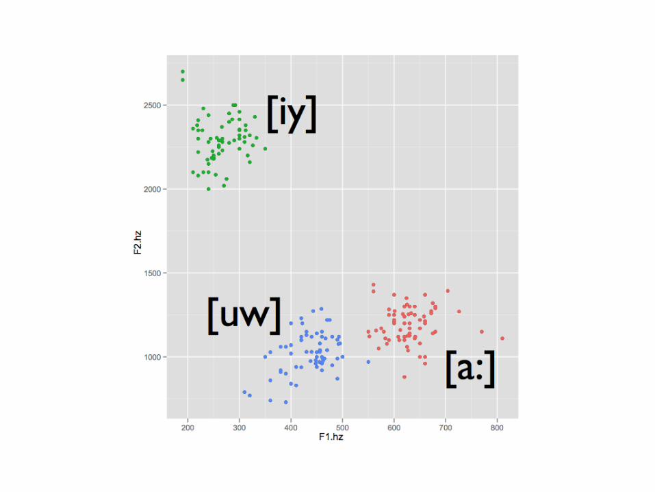


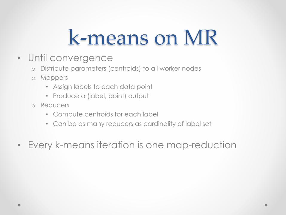
k-‐‑means on MR • Until convergence
o Distribute parameters (centroids) to all worker nodes o Mappers
• Assign labels to each data point • Produce a (label, point) output
o Reducers • Compute centroids for each label
• Can be as many reducers as cardinality of label set
• Every k-means iteration is one map-reduction
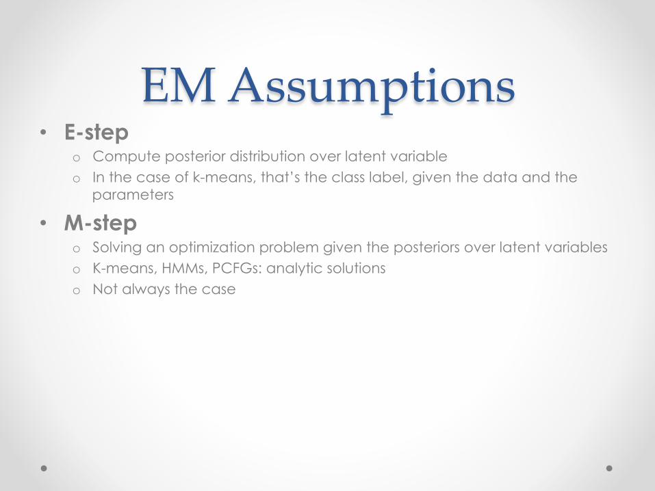
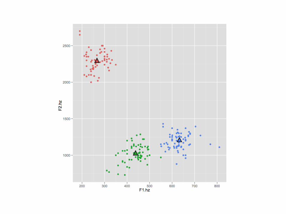
EM Assumptions • E-step
o Compute posterior distribution over latent variable o In the case of k-means, that’s the class label, given the data and the
parameters
• M-step o Solving an optimization problem given the posteriors over latent variables o K-means, HMMs, PCFGs: analytic solutions o Not always the case
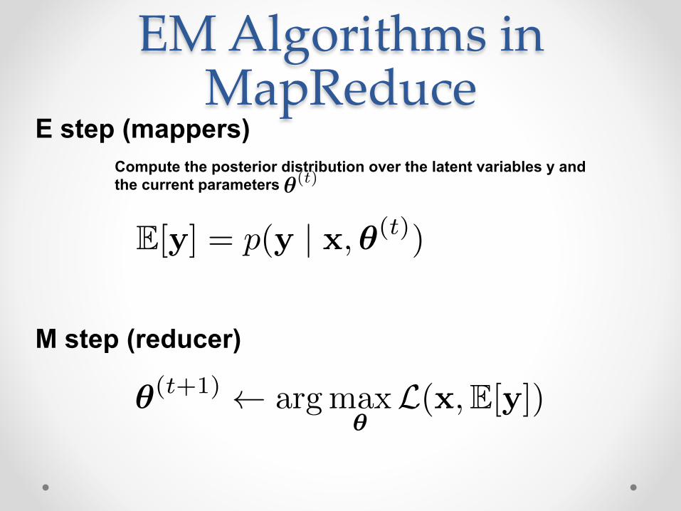
Compute the posterior distribution over the latent variables y and the current parameters
E step (mappers)
M step (reducer)
EM Algorithms in MapReduce
✓(t)
✓(t+1) argmax
✓L(x,E[y])
E[y] = p(y | x,✓(t))

Compute the posterior distribution over the latent variables y and the current parameters
EM Algorithms in MapReduce
✓(t)
Cluster labels Data points
✓(t+1) argmax
✓L(x,E[y])
E[y] = p(y | x,✓(t))
E step (mappers)
M step (reducer)
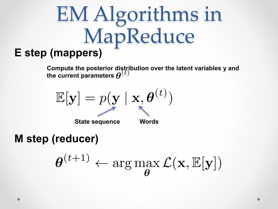
Compute the posterior distribution over the latent variables y and the current parameters
EM Algorithms in MapReduce
✓(t)
State sequence Words
✓(t+1) argmax
✓L(x,E[y])
E[y] = p(y | x,✓(t))
E step (mappers)
M step (reducer)

Compute the expected log likelihood with respect to the conditional distribution of the latent variables with respect to the observed data.
E step
Expectations are just sums of function evaluation over an event times that event’s probability: perfect for MapReduce!
Mappers compute model likelihood given small pieces of the training data (scale EM to large data sets!)
EM Algorithms in MapReduce
E[y] = p(y | x,✓(t))
M step
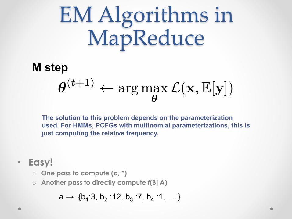
The solution to this problem depends on the parameterization used. For HMMs, PCFGs with multinomial parameterizations, this is just computing the relative frequency.
EM Algorithms in MapReduce
✓(t+1) argmax
✓L(x,E[y])
• Easy! o One pass to compute (a, *) o Another pass to directly compute f(B|A)
a → {b1:3, b2 :12, b3 :7, b4 :1, … }
Challenges • Each iteration of EM is one MapReduce job • Mappers require the current model parameters
o Certain models may be very large o Optimization: any particular piece of the training data probably depends
on only a small subset of these parameters
• Reducers may aggregate data from many mappers o Optimization: Make smart use of combiners!

Log-‐‑linear Models • NLP’s favorite discriminative model:
• Applied successfully to classificiation, POS tagging, parsing, MT, word segmentation, named entity recognition, LM… o Make use of millions of features (hi’s) o Features may overlap o Global optimum easily reachable, assuming no latent variables
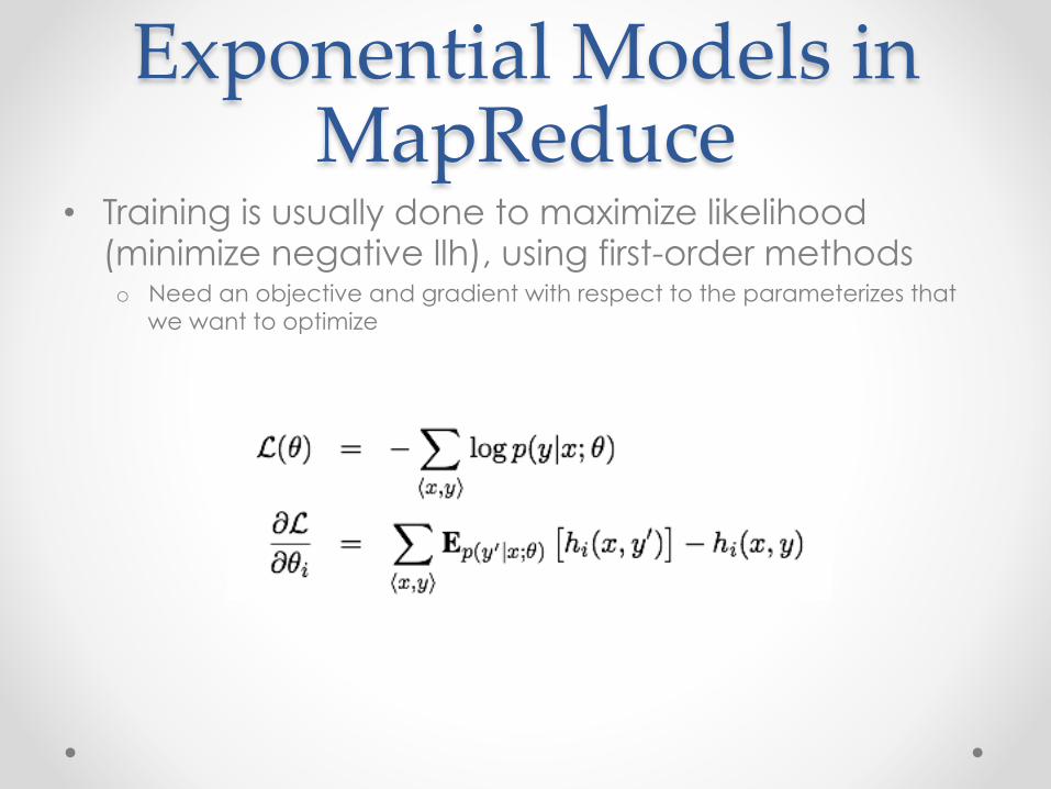
Exponential Models in MapReduce
• Training is usually done to maximize likelihood (minimize negative llh), using first-order methods o Need an objective and gradient with respect to the parameterizes that
we want to optimize

Exponential Models in MapReduce
• How do we compute these in MapReduce?
As seen with EM: expectations map nicely onto the MR paradigm.
Each mapper computes two quantities: the LLH of a training instance <x,y> under the current model and the contribution to the gradient.
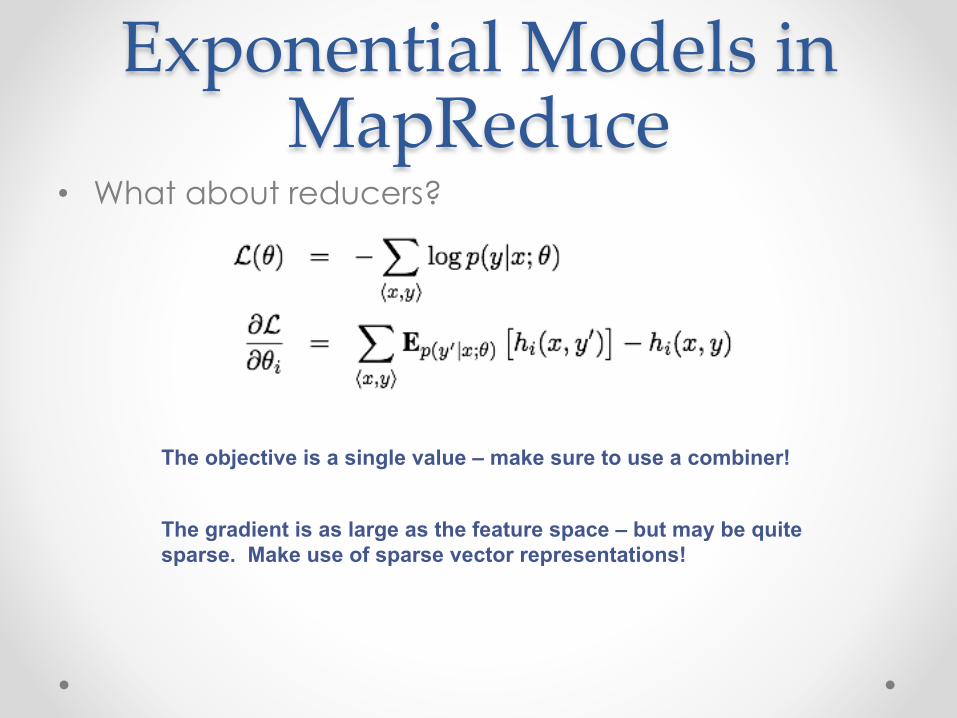
Exponential Models in MapReduce
• What about reducers?
The objective is a single value – make sure to use a combiner!
The gradient is as large as the feature space – but may be quite sparse. Make use of sparse vector representations!
Exponential Models in MapReduce
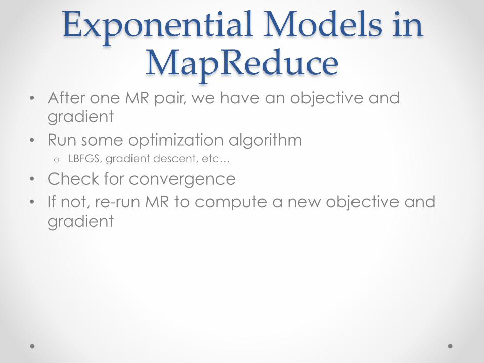
• After one MR pair, we have an objective and gradient
• Run some optimization algorithm o LBFGS, gradient descent, etc…
• Check for convergence • If not, re-run MR to compute a new objective and
gradient

Challenges • Each iteration of training is one MapReduce job • Mappers require the current model parameters • Reducers may aggregate data from many
mappers • Optimization algorithm (LBFGS for example) may
require the full gradient o This is okay for millions of features o What about billions? o …or trillions?

Case study: statistical machine translation
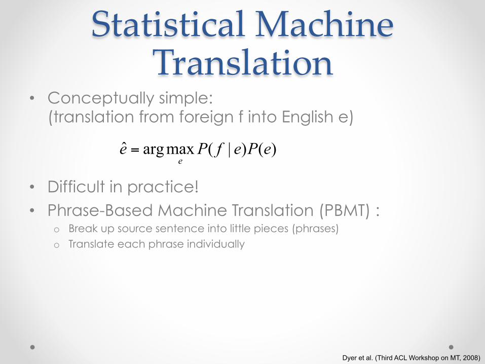
Statistical Machine Translation
• Conceptually simple: (translation from foreign f into English e)
• Difficult in practice! • Phrase-Based Machine Translation (PBMT) :
o Break up source sentence into little pieces (phrases) o Translate each phrase individually
)()|(maxargˆ ePefPee
=
Dyer et al. (Third ACL Workshop on MT, 2008)

Maria no dio una bofetada a la bruja verde
Mary not
did not
no
did not give
give a slap to the witch green
slap
slap
a slap
to the
to
the
green witch
the witch
by
Example from Koehn (2006)
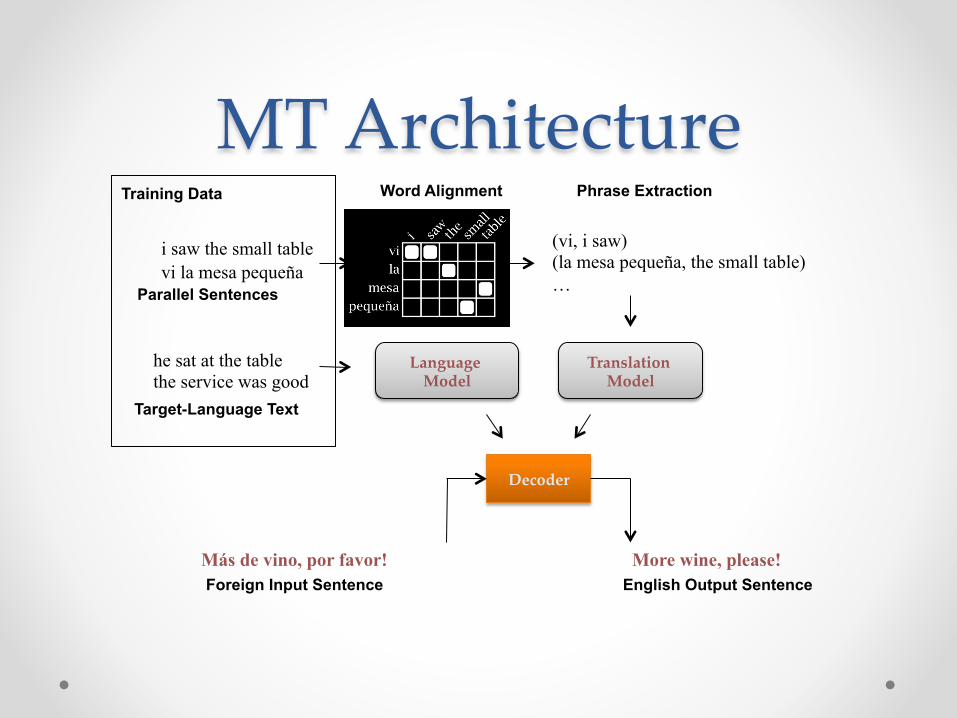
i saw the small table vi la mesa pequeña
(vi, i saw) (la mesa pequeña, the small table) … Parallel Sentences
Word Alignment Phrase Extraction
he sat at the table the service was good
Target-Language Text
Translation Model
Language Model
Decoder
Foreign Input Sentence English Output Sentence Más de vino, por favor! More wine, please!
Training Data
MT Architecture
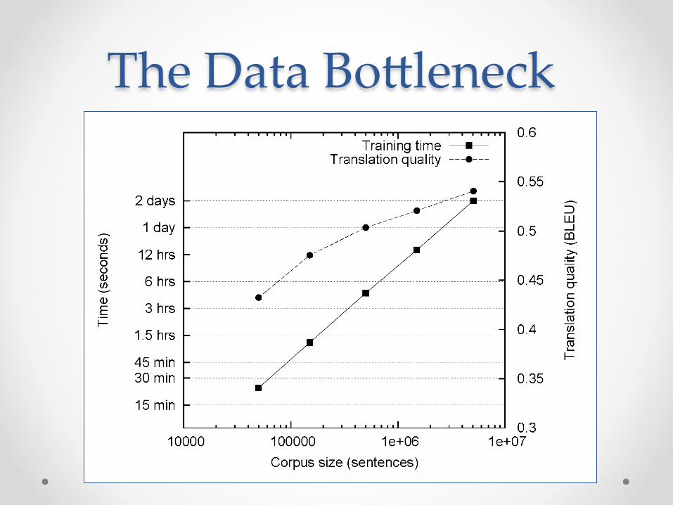
The Data Bo]leneck
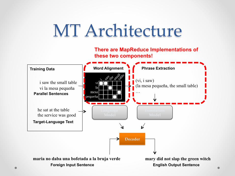
i saw the small table vi la mesa pequeña
(vi, i saw) (la mesa pequeña, the small table) … Parallel Sentences
Word Alignment Phrase Extraction
he sat at the table the service was good
Target-Language Text
Translation Model
Language Model
Decoder
Foreign Input Sentence English Output Sentence maria no daba una bofetada a la bruja verde mary did not slap the green witch
Training Data
MT Architecture There are MapReduce Implementations of these two components!

Alignment with HMMs
Mary slapped the green witch
Mary deu um tapa a bruxa verde 1 2 3 4 5 6 7
Vogel et al. (1996)
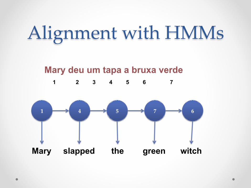
Alignment with HMMs
1 4 5 7 6
Mary slapped the green witch
Mary deu um tapa a bruxa verde 1 2 3 4 5 6 7
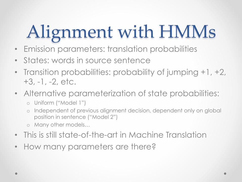
Alignment with HMMs • Emission parameters: translation probabilities • States: words in source sentence • Transition probabilities: probability of jumping +1, +2,
+3, -1, -2, etc. • Alternative parameterization of state probabilities:
o Uniform (“Model 1”) o Independent of previous alignment decision, dependent only on global
position in sentence (“Model 2”) o Many other models…
• This is still state-of-the-art in Machine Translation • How many parameters are there?

HMM Alignment: Giza
Single-core commodity server
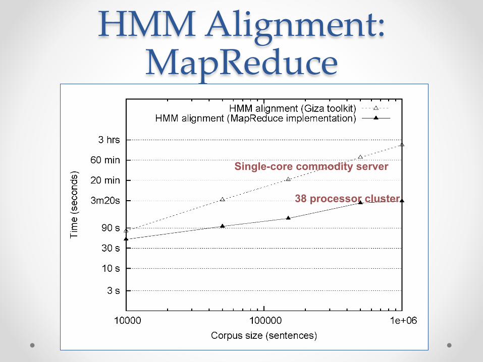
HMM Alignment: MapReduce
38 processor cluster
Single-core commodity server

HMM Alignment: MapReduce
38 processor cluster
1/38 Single-core commodity server

Online Learning Algorithms in MR
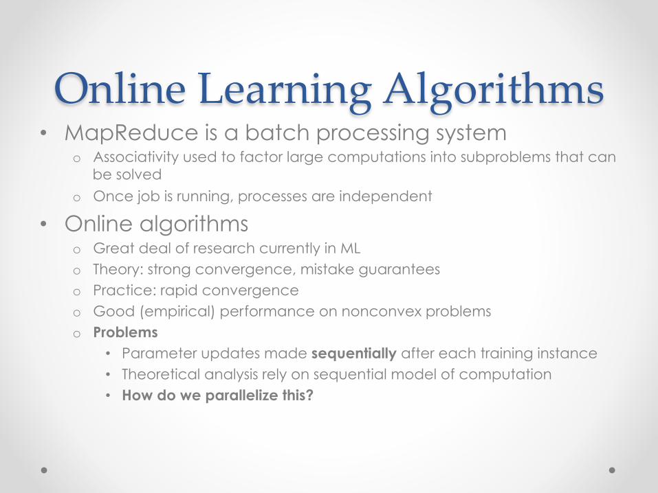
Online Learning Algorithms • MapReduce is a batch processing system
o Associativity used to factor large computations into subproblems that can be solved
o Once job is running, processes are independent
• Online algorithms o Great deal of research currently in ML o Theory: strong convergence, mistake guarantees o Practice: rapid convergence o Good (empirical) performance on nonconvex problems o Problems
• Parameter updates made sequentially after each training instance • Theoretical analysis rely on sequential model of computation • How do we parallelize this?

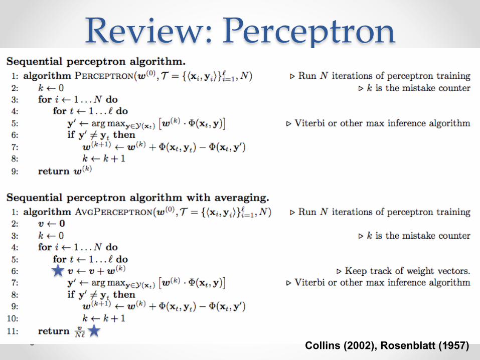
Review: Perceptron
Collins (2002), Rosenblatt (1957)
Review: Perceptron
Collins (2002), Rosenblatt (1957)
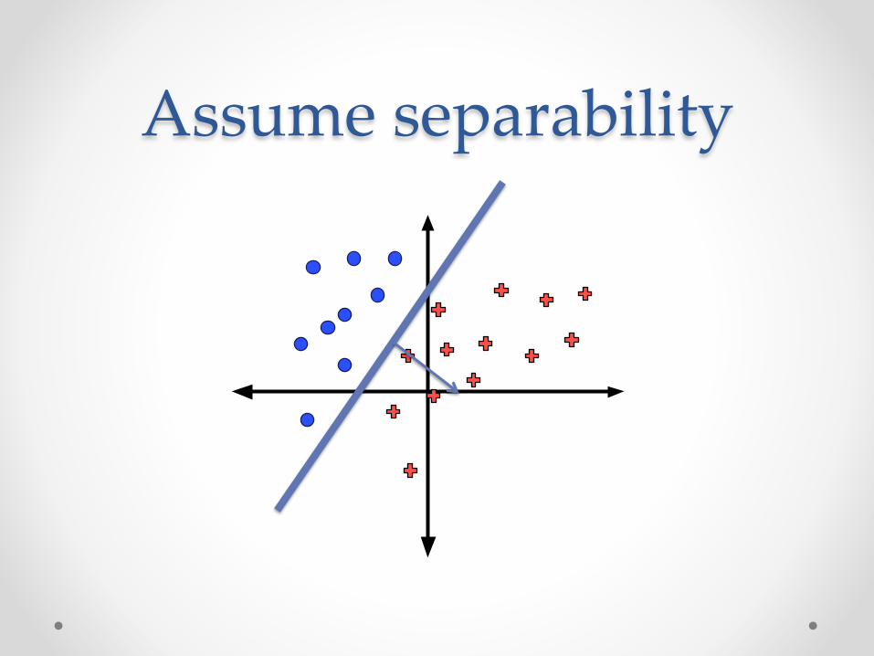
Assume separability

Algorithm 1: Parameter Mixing • Inspired by the averaged perceptron, let’s run P
perceptrons on shards of the data • Return the average parameters
Return average parameters from P runs
McDonald, Hall, & Mann (NAACL, 2010)

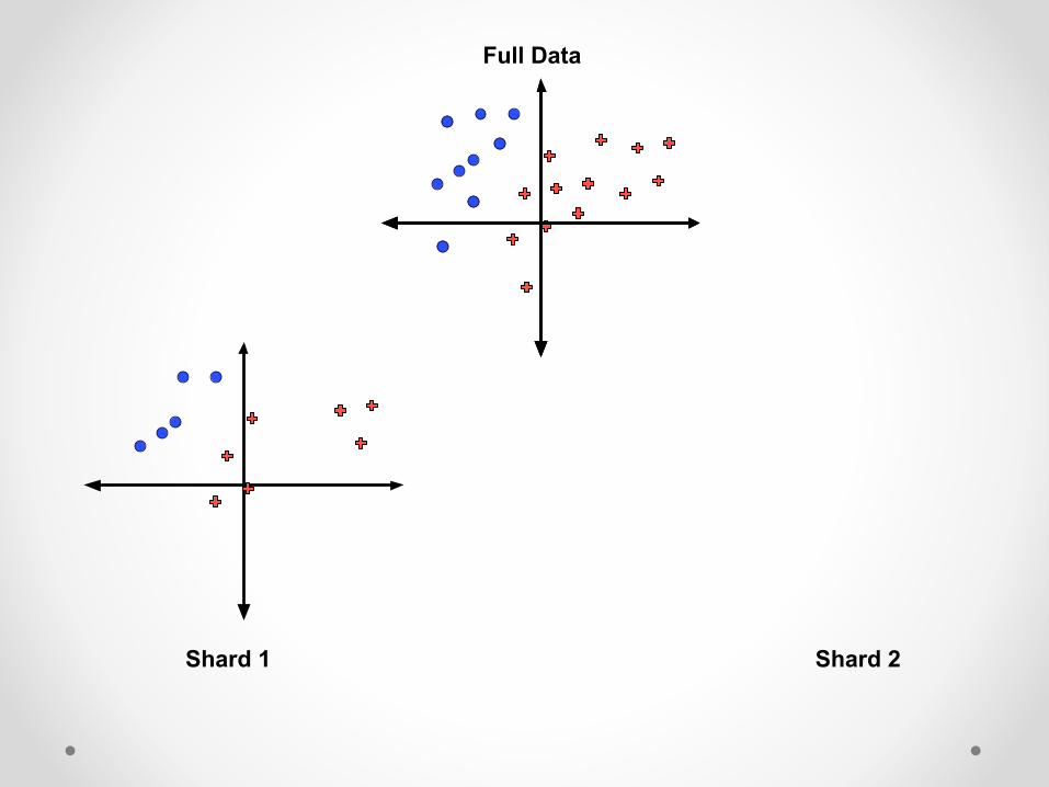
Full Data
Shard 1 Shard 2
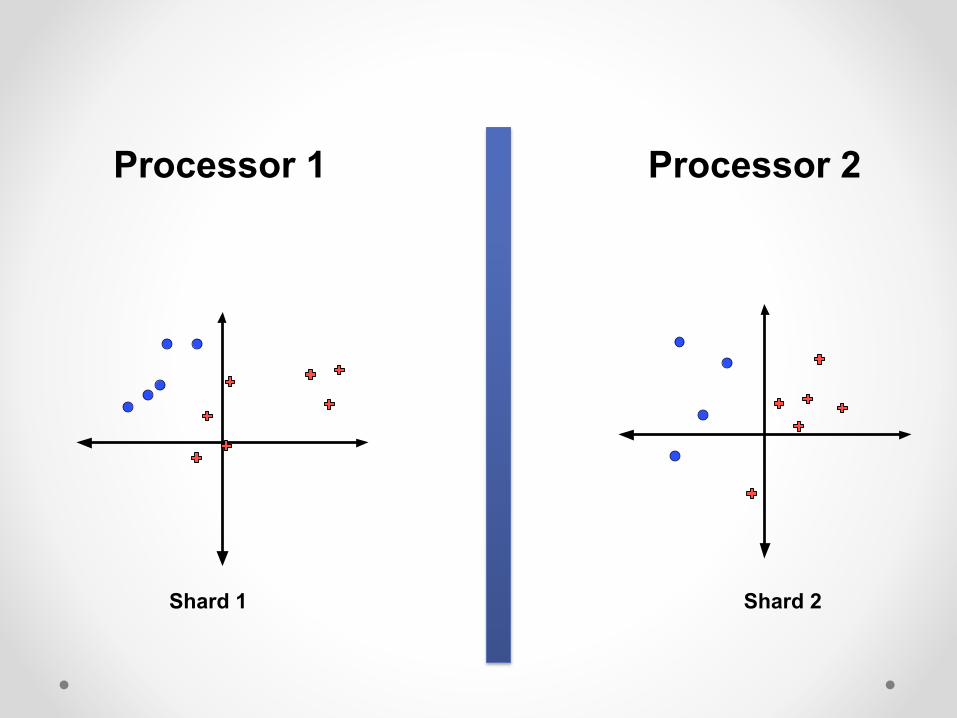
Shard 1 Shard 2
Processor 1 Processor 2
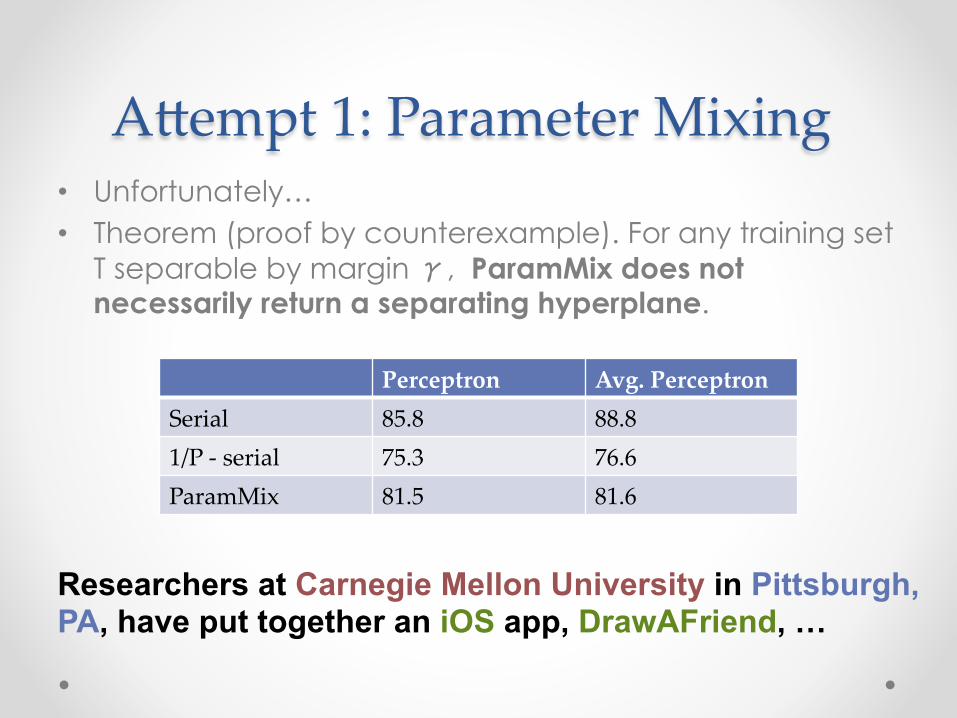
A]empt 1: Parameter Mixing • Unfortunately… • Theorem (proof by counterexample). For any training set
T separable by margin γ, ParamMix does not necessarily return a separating hyperplane.
Perceptron Avg. Perceptron Serial 85.8 88.8 1/P -‐‑ serial 75.3 76.6 ParamMix 81.5 81.6
Researchers at Carnegie Mellon University in Pittsburgh, PA, have put together an iOS app, DrawAFriend, …
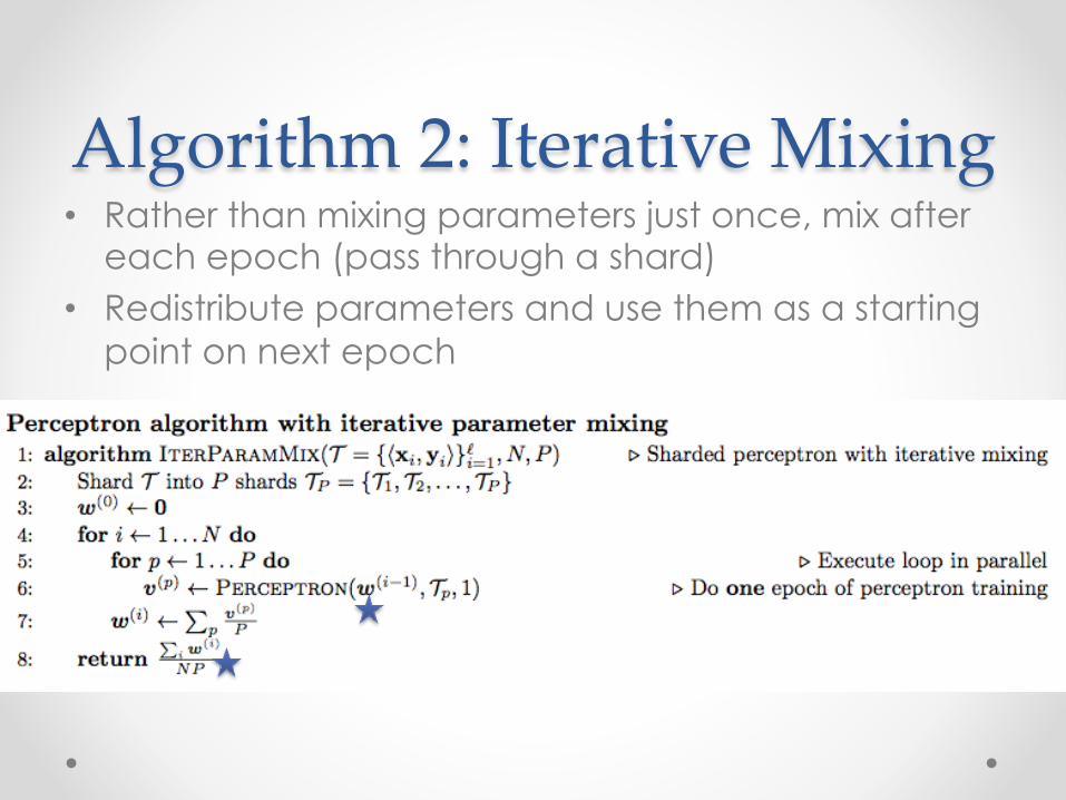
Algorithm 2: Iterative Mixing • Rather than mixing parameters just once, mix after
each epoch (pass through a shard) • Redistribute parameters and use them as a starting
point on next epoch
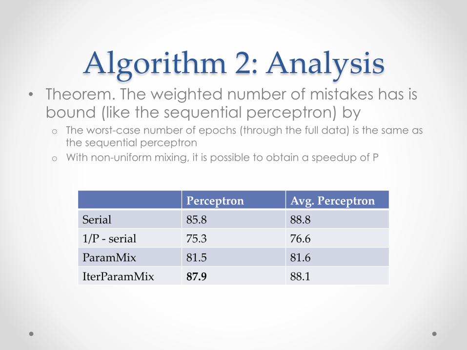
Algorithm 2: Analysis • Theorem. The weighted number of mistakes has is
bound (like the sequential perceptron) by o The worst-case number of epochs (through the full data) is the same as
the sequential perceptron o With non-uniform mixing, it is possible to obtain a speedup of P
Perceptron Avg. Perceptron Serial 85.8 88.8 1/P -‐‑ serial 75.3 76.6 ParamMix 81.5 81.6 IterParamMix 87.9 88.1
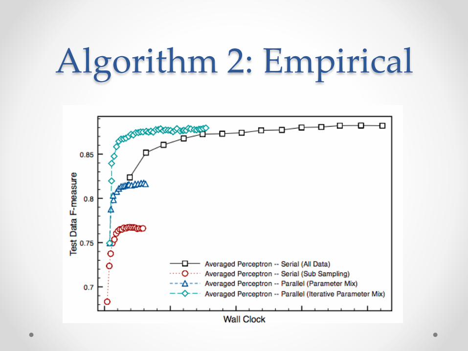
Algorithm 2: Empirical
Summary • Two approaches to learning
o Batch: process the entire dataset and make a single update o Online: sequential updates
• Online learning is hard to realize in a distributed (parallelized) environment o Parameter mixing approaches offer a theoretically sound solution with
practical performance guarantees o Generalizations to log-loss and MIRA loss have also been explored o Conceptually some workers have “stale parameters” that eventually
(after a number of synchronizations) reflect the true state of the learner
• Other challenges (next couple of days) o Large numbers of parameters (randomized representations) o Large numbers of related tasks (multitask learning)

Obrigado!