Learning towards Minimum Hyperspherical Energy

Weiyang Liu1,*, Rongmei Lin2,*, Zhen Liu1,*, Lixin Liu3,*, Zhiding Yu4, Bo Dai1,5, Le Song1,6

1Georgia Institute of Technology 2Emory University3South China University of Technology 4NVIDIA 5Google Brain 6Ant Financial

Abstract

Neural networks are a powerful class of nonlinear functions that can be trainedend-to-end on various applications. While the over-parametrization nature inmany neural networks renders the ability to fit complex functions and the strongrepresentation power to handle challenging tasks, it also leads to highly correlatedneurons that can hurt the generalization ability and incur unnecessary computationcost. As a result, how to regularize the network to avoid undesired representationredundancy becomes an important issue. To this end, we draw inspiration from awell-known problem in physics – Thomson problem, where one seeks to find a statethat distributes N electrons on a unit sphere as evenly as possible with minimumpotential energy. In light of this intuition, we reduce the redundancy regularizationproblem to generic energy minimization, and propose a minimum hypersphericalenergy (MHE) objective as generic regularization for neural networks. We alsopropose a few novel variants of MHE, and provide some insights from a theoreticalpoint of view. Finally, we apply neural networks with MHE regularization toseveral challenging tasks. Extensive experiments demonstrate the effectiveness ofour intuition, by showing the superior performance with MHE regularization.

1 Introduction

The recent success of deep neural networks has led to its wide applications in a variety of tasks. Withthe over-parametrization nature and deep layered architecture, current deep networks [15, 47, 43]are able to achieve impressive performance on large-scale problems. Despite such success, havingredundant and highly correlated neurons (e.g., weights of kernels/filters in convolutional neuralnetworks (CNNs)) caused by over-parametrization presents an issue [38, 42], which motivated a seriesof influential works in network compression [11, 1] and parameter-efficient network architectures [17,20, 64]. These works either compress the network by pruning redundant neurons or directly modifythe network architecture, aiming to achieve comparable performance while using fewer parameters.Yet, it remains an open problem to find a unified and principled theory that guides the networkcompression in the context of optimal generalization ability.

Another stream of works seeks to further release the network generalization power by alleviatingredundancy through diversification [59, 58, 5, 37] as rigorously analyzed by [61]. Most of theseworks address the redundancy problem by enforcing relatively large diversity between pairwiseprojection bases via regularization. Our work broadly falls into this category by sharing similarhigh-level target, but the spirit and motivation behind our proposed models are distinct. In particular,there is a recent trend of studies that feature the significance of angular learning at both loss andconvolution levels [30, 29, 31, 28], based on the observation that the angles in deep embeddingslearned by CNNs tend to encode semantic difference. The key intuition is that angles preserve themost abundant and discriminative information for visual recognition. As a result, hypersphericalgeodesic distances between neurons naturally play a key role in this context, and thus, it is intuitivelydesired to impose discrimination by keeping their projections on the hypersphere as far away from

* indicates equal contributions. Correspondence to: Weiyang Liu <wyliu@gatech.edu>.

32nd Conference on Neural Information Processing Systems (NeurIPS 2018), Montréal, Canada.

arX

iv:1

805.

0929

8v8

[cs

.LG

] 5

Mar

201

9

each other as possible. While the concept of imposing large angular diversities was also consideredin [61, 59, 58, 37], they do not consider diversity in terms of global equidistribution of embeddingson the hypersphere, which fails to achieve the state-of-the-art performances.

Given the above motivation, we draw inspiration from a well-known physics problem, called Thomsonproblem [49, 44]. The goal of Thomson problem is to determine the minimum electrostatic potentialenergy configuration of N mutually-repelling electrons on the surface of a unit sphere. We identifythe intrinsic resemblance between the Thomson problem and our target, in the sense that diversifyingneurons can be seen as searching for an optimal configuration of electron locations. Similarly, wecharacterize the diversity for a group of neurons by defining a generic hyperspherical potential energyusing their pairwise relationship. Higher energy implies higher redundancy, while lower energyindicates that these neurons are more diverse and more uniformly spaced. To reduce the redundancyof neurons and improve the neural networks, we propose a novel minimum hyperspherical energy(MHE) regularization framework, where the diversity of neurons is promoted by minimizing thehyperspherical energy in each layer. As verified by comprehensive experiments on multiple tasks,MHE is able to consistently improve the generalization power of neural networks.

Orthonormal MHE Half-space MHE

Figure 1: Orthonormal, MHE and half-space MHE regularization.The red dots denote the neurons optimized by the gradient of thecorresponding regularization. The rightmost pink dots denotethe virtual negative neurons. We randomly initialize the weightsof 10 neurons on a 3D Sphere and optimize them with SGD.

MHE faces different situations when it isapplied to hidden layers and output lay-ers. For hidden layers, applying MHEstraightforwardly may still encouragesome degree of redundancy since it willproduce co-linear bases pointing to op-posite directions (see Fig. 1 middle). Inorder to avoid such redundancy, we pro-pose the half-space MHE which con-structs a group of virtual neurons andminimize the hyperspherical energy ofboth existing and virtual neurons. Foroutput layers, MHE aims to distributethe classifier neurons1 as uniformly aspossible to improve the inter-class feature separability. Different from MHE in hidden layers, classi-fier neurons should be distributed in the full space for the best classification performance [30, 29].An intuitive comparison among the widely used orthonormal regularization, the proposed MHE andhalf-space MHE is provided in Fig. 1. One can observe that both MHE and half-space MHE are ableto uniformly distribute the neurons over the hypersphere and half-space hypershpere, respectively. Incontrast, conventional orthonormal regularization tends to group neurons closer, especially when thenumber of neurons is greater than the dimension.MHE is originally defined on Euclidean distance, as indicated in Thomson problem. However, wefurther consider minimizing hyperspherical energy defined with respect to angular distance, which wewill refer to as angular-MHE (A-MHE) in the following paper. In addition, we give some theoreticalinsights of MHE regularization, by discussing the asymptotic behavior and generalization error.Last, we apply MHE regularization to multiple vision tasks, including generic object recognition,class-imbalance learning, and face recognition. In the experiments, we show that MHE is architecture-agnostic and can considerably improve the generalization ability.

2 Related WorksDiversity regularization is shown useful in sparse coding [33, 36], ensemble learning [27, 25], self-paced learning [22], metric learning [60], etc. Early studies in sparse coding [33, 36] show that thegeneralization ability of codebook can be improved via diversity regularization, where the diversityis often modeled using the (empirical) covariance matrix. More recently, a series of studies havefeatured diversity regularization in neural networks [61, 59, 58, 5, 37, 57], where regularization ismostly achieved via promoting large angle/orthogonality, or reducing covariance between bases. Ourwork differs from these studies by formulating the diversity of neurons on the entire hypersphere,therefore promoting diversity from a more global, top-down perspective.Methods other than diversity-promoting regularization have been widely proposed to improveCNNs [45, 21, 34, 31] and generative adversarial nets (GANs) [4, 35]. MHE can be regardedas a complement that can be applied on top of these methods.

1Classifier neurons are the projection bases of the last layer (i.e., output layer) before input to softmax.

2

3 Learning Neurons towards Minimum Hyperspherical Energy3.1 Formulation of Minimum Hyperspherical EnergyMinimum hyperspherical energy defines an equilibrium state of the configuration of neuron’s direc-tions. We argue that the power of neural representation of each layer can be characterized by thehyperspherical energy of its neurons, and therefore a minimal energy configuration of neurons caninduce better generalization. Before delving into details, we first define the hyperspherical energyfunctional for N neurons (i.e., kernels) with (d+1)-dimension WN ={w1, · · · ,wN ∈Rd+1} as

Es,d(wi|Ni=1) =

N∑i=1

N∑j=1,j 6=i

fs(‖wi − wj‖

)=

{ ∑i 6=j ‖wi − wj‖−s , s > 0∑i 6=j log

(‖wi − wj‖−1 ), s = 0

, (1)

where ‖·‖ denotes Euclidean distance, fs(·) is a decreasing real-valued function, and wi=wi

‖wi‖is the i-th neuron weight projected onto the unit hypersphere Sd={w∈Rd+1| ‖w‖=1}. We alsodenote WN ={w1, · · · , wN ∈Sd}, and Es=Es,d(wi|Ni=1) for short. There are plenty of choices forfs(·), but in this paper we use fs(z) = z−s, s > 0, known as Riesz s-kernels. Particularly, as s→ 0,z−s→s log(z−1)+1, which is an affine transformation of log(z−1). It follows that optimizing thelogarithmic hyperspherical energy E0 =

∑i 6=j log(‖wi−wj‖−1) is essentially the limiting case of

optimizing the hyperspherical energy Es. We therefore define f0(z)=log(z−1) for convenience.

The goal of the MHE criterion is to minimize the energy in Eq. (1) by varying the orientations of theneuron weights w1, · · · ,wN . To be precise, we solve an optimization problem: minWN

Es withs ≥ 0. In particular, when s=0, we solve the logarithmic energy minimization problem:

argminWN

E0 = argminWN

exp(E0) = argmaxWN

∏i 6=j

‖wi − wj‖ , (2)

in which we essentially maximize the product of Euclidean distances. E0, E1 and E2 have interestingyet profound connections. Note that Thomson problem corresponds to minimizing E1, which is aNP-hard problem. Therefore in practice we can only compute its approximate solution by heuristics.In neural networks, such a differentiable objective can be directly optimized via gradient descent.

3.2 Logarithmic Hyperspherical Energy E0 as a RelaxationOptimizing the original energy in Eq. (1) is equivalent to optimizing its logarithmic form logEs.To efficiently solve this difficult optimization problem, we can instead optimize the lower bound oflogEs as a surrogate energy, by applying Jensen’s inequality:

argminWN

{Elog :=

N∑i=1

N∑j=1,j 6=i

log

(fs(‖wi − wj‖

))}(3)

With fs(z)=z−s, s>0, we observe that Elog becomes sE0 =s∑i 6=j log(‖wi−wj‖−1), which is

identical to the logarithmic hyperspherical energy E0 up to a multiplicative factor s. Therefore,minimizing E0 can also be viewed as a relaxation of minimizing Es for s>0.

3.3 MHE as Regularization for Neural NetworksNow that we have introduced the formulation of MHE, we propose MHE regularization for neuralnetworks. In supervised neural network learning, the entire objective function is shown as follows:

L =1

m

m∑j=1

`(〈wouti ,xj〉ci=1,yj)︸ ︷︷ ︸

training data fitting

+ λh ·L−1∑j=1

1

Nj(Nj − 1){Es}j︸ ︷︷ ︸

Th: hyperspherical energy for hidden layers

+λo ·1

NL(NL − 1)Es(w

outi |ci=1)︸ ︷︷ ︸

To: hyperspherical energy for output layer

(4)

where xi is the feature of the i-th training sample entering the output layer, wouti is the classifier

neuron for the i-th class in the output fully-connected layer and wouti denotes its normalized version.

{Es}i denotes the hyperspherical energy for the neurons in the i-th layer. c is the number of classes,m is the batch size, L is the number of layers of the neural network, and Ni is the number of neuronsin the i-th layer. Es(w

outi |ci=1) denotes the hyperspherical energy of neurons {wout

1 , · · · , woutc }.

The `2 weight decay is omitted here for simplicity, but we will use it in practice. An alternativeinterpretation of MHE regularization from a decoupled view is given in Section 3.7 and Appendix C.MHE has different effects and interpretations in regularizing hidden layers and output layers.

MHE for hidden layers. To make neurons in the hidden layers more discriminative and less redun-dant, we propose to use MHE as a form of regularization. MHE encourages the normalized neurons to

3

be uniformly distributed on a unit hypersphere, which is partially inspired by the observation in [31]that angular difference in neurons preserves semantic (label-related) information. To some extent,MHE maximizes the average angular difference between neurons (specifically, the hypersphericalenergy of neurons in every hidden layer). For instance, in CNNs we minimize the hyperpshericalenergy of kernels in convolutional and fully-connected layers except the output layer.

MHE for output layers. For the output layer, we propose to enhance the inter-class feature separa-bility with MHE to learn discriminative and well-separated features. For classification tasks, MHEregularization is complementary to the softmax cross-entropy loss in CNNs. The softmax loss focusesmore on the intra-class compactness, while MHE encourages the inter-class separability. Therefore,MHE on output layers can induce features with better generalization power.

3.4 MHE in Half Space

Original MHE Half-space MHE

w1

w2

w1

w2

-w1

-w2

^

^

^

^

^

^

Figure 2: Half-space MHE.

Directly applying the MHE formulation may still encouter someredundancy. An example in Fig. 2, with two neurons in a 2-dimensional space, illustrates this potential issue. Directly im-posing the original MHE regularization leads to a solution thattwo neurons are colinear but with opposite directions. To avoidsuch redundancy, we propose the half-space MHE regularizationwhich constructs some virtual neurons and minimizes the hyper-spherical energy of both original and virtual neurons together.Specifically, half-space MHE constructs a colinear virtual neuron with opposite direction for everyexisting neuron. Therefore, we end up with minimizing the hyperspherical energy with 2Ni neuronsin the i-th layer (i.e., minimizing Es({wk,−wk}|2Ni

k=1)). This half-space variant will encourage theneurons to be less correlated and less redundant, as illustrated in Fig. 2. Note that, half-space MHEcan only be used in hidden layers, because the colinear neurons do not constitute redundancy in outputlayers, as shown in [30]. Nevertheless, colinearity is usually not likely to happen in high-dimensionalspaces, especially when the neurons are optimized to fit training data. This may be the reason that theoriginal MHE regularization still consistently improves the baselines.

3.5 MHE beyond Euclidean DistanceThe hyperspherical energy is originally defined based on the Euclidean distance on a hypersphere,which can be viewed as an angular measure. In addition to Euclidean distance, we further considerthe geodesic distance on a unit hypersphere as a distance measure for neurons, which is exactlythe same as the angle between neurons. Specifically, we consider to use arccos(w>i wj) to replace‖wi−wj‖ in hyperspherical energies. Following this idea, we propose angular MHE (A-MHE) as asimple extension, where the hyperspherical energy is rewritten as:

Eas,d(wi|Ni=1) =

N∑i=1

N∑j=1,j 6=i

fs(arccos(w>i wj)

)=

{ ∑i6=j arccos(w

>i wj)

−s, s > 0∑i6=j log

(arccos(w>i wj)

−1), s = 0

(5)

which can be viewed as redefining MHE based on geodesic distance on hyperspheres (i.e., angle), andcan be used as an alternative to the original hyperspherical energy Es in Eq. (4). Note that, A-MHEcan also be learned in full-space or half-space, leading to similar variants as original MHE. The keydifference between MHE and A-MHE lies in the optimization dynamics, because their gradients w.r.tthe neuron weights are quite different. A-MHE is also more computationally expensive than MHE.

3.6 Mini-batch Approximation for MHEWith a large number of neurons in one layer, calculating MHE can be computationally expensive as itrequires computing the pair-wise distances between neurons. To address this issue, we propose themini-batch version of MHE to approximate the MHE (either original or half-space) objective.Mini-batch approximation for MHE on hidden layers. For hidden layers, mini-batch approxima-tion iteratively takes a random batch of neurons as input and minimizes their hyperspherical energyas an approximation to the MHE. Note that the gradient of the mini-batch objective is an unbiasedestimation of the original gradient of MHE.Data-dependent mini-batch approximation for output layers. For the output layer, the data-dependent mini-batch approximation iteratively takes the classifier neurons corresponding to theclasses that exist in mini-batches. It minimizes 1

m(N−1)∑mi=1

∑Nj=1,j 6=yi fs(‖wyi − wj‖) in each

iteration, where yi denotes the class label of the i-th sample in each mini-batch, m is the mini-batchsize, and N is the number of neurons (in one particular layer).

4

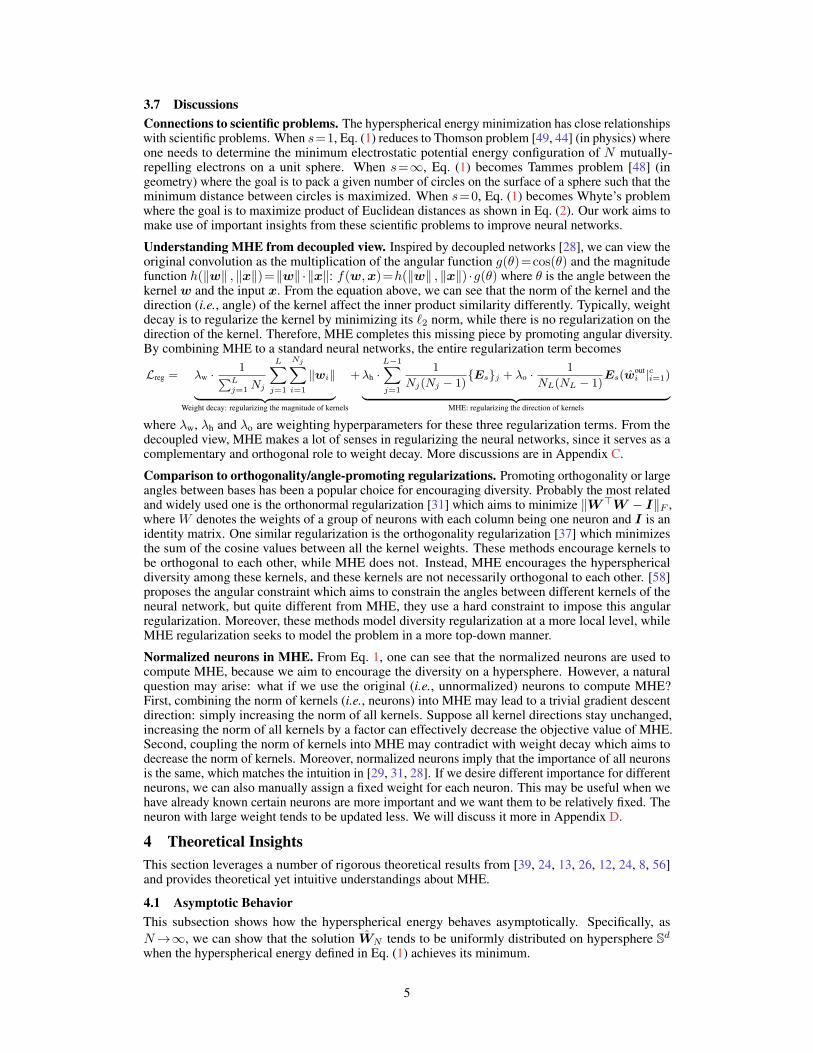
3.7 DiscussionsConnections to scientific problems. The hyperspherical energy minimization has close relationshipswith scientific problems. When s=1, Eq. (1) reduces to Thomson problem [49, 44] (in physics) whereone needs to determine the minimum electrostatic potential energy configuration of N mutually-repelling electrons on a unit sphere. When s=∞, Eq. (1) becomes Tammes problem [48] (ingeometry) where the goal is to pack a given number of circles on the surface of a sphere such that theminimum distance between circles is maximized. When s=0, Eq. (1) becomes Whyte’s problemwhere the goal is to maximize product of Euclidean distances as shown in Eq. (2). Our work aims tomake use of important insights from these scientific problems to improve neural networks.

Understanding MHE from decoupled view. Inspired by decoupled networks [28], we can view theoriginal convolution as the multiplication of the angular function g(θ)=cos(θ) and the magnitudefunction h(‖w‖ , ‖x‖)=‖w‖·‖x‖: f(w,x)=h(‖w‖ , ‖x‖) ·g(θ) where θ is the angle between thekernel w and the input x. From the equation above, we can see that the norm of the kernel and thedirection (i.e., angle) of the kernel affect the inner product similarity differently. Typically, weightdecay is to regularize the kernel by minimizing its `2 norm, while there is no regularization on thedirection of the kernel. Therefore, MHE completes this missing piece by promoting angular diversity.By combining MHE to a standard neural networks, the entire regularization term becomes

Lreg = λw ·1∑L

j=1Nj

L∑j=1

Nj∑i=1

‖wi‖︸ ︷︷ ︸Weight decay: regularizing the magnitude of kernels

+λh ·L−1∑j=1

1

Nj(Nj − 1){Es}j + λo ·

1

NL(NL − 1)Es(w

outi |ci=1)︸ ︷︷ ︸

MHE: regularizing the direction of kernels

where λw, λh and λo are weighting hyperparameters for these three regularization terms. From thedecoupled view, MHE makes a lot of senses in regularizing the neural networks, since it serves as acomplementary and orthogonal role to weight decay. More discussions are in Appendix C.

Comparison to orthogonality/angle-promoting regularizations. Promoting orthogonality or largeangles between bases has been a popular choice for encouraging diversity. Probably the most relatedand widely used one is the orthonormal regularization [31] which aims to minimize ‖W>W − I‖F ,where W denotes the weights of a group of neurons with each column being one neuron and I is anidentity matrix. One similar regularization is the orthogonality regularization [37] which minimizesthe sum of the cosine values between all the kernel weights. These methods encourage kernels tobe orthogonal to each other, while MHE does not. Instead, MHE encourages the hypersphericaldiversity among these kernels, and these kernels are not necessarily orthogonal to each other. [58]proposes the angular constraint which aims to constrain the angles between different kernels of theneural network, but quite different from MHE, they use a hard constraint to impose this angularregularization. Moreover, these methods model diversity regularization at a more local level, whileMHE regularization seeks to model the problem in a more top-down manner.

Normalized neurons in MHE. From Eq. 1, one can see that the normalized neurons are used tocompute MHE, because we aim to encourage the diversity on a hypersphere. However, a naturalquestion may arise: what if we use the original (i.e., unnormalized) neurons to compute MHE?First, combining the norm of kernels (i.e., neurons) into MHE may lead to a trivial gradient descentdirection: simply increasing the norm of all kernels. Suppose all kernel directions stay unchanged,increasing the norm of all kernels by a factor can effectively decrease the objective value of MHE.Second, coupling the norm of kernels into MHE may contradict with weight decay which aims todecrease the norm of kernels. Moreover, normalized neurons imply that the importance of all neuronsis the same, which matches the intuition in [29, 31, 28]. If we desire different importance for differentneurons, we can also manually assign a fixed weight for each neuron. This may be useful when wehave already known certain neurons are more important and we want them to be relatively fixed. Theneuron with large weight tends to be updated less. We will discuss it more in Appendix D.

4 Theoretical InsightsThis section leverages a number of rigorous theoretical results from [39, 24, 13, 26, 12, 24, 8, 56]and provides theoretical yet intuitive understandings about MHE.

4.1 Asymptotic BehaviorThis subsection shows how the hyperspherical energy behaves asymptotically. Specifically, asN→∞, we can show that the solution WN tends to be uniformly distributed on hypersphere Sdwhen the hyperspherical energy defined in Eq. (1) achieves its minimum.

5

Definition 1 (minimal hyperspherical s-energy). We define the minimal s-energy for N points on theunit hypersphere Sd={w∈Rd+1| ‖w‖=1} as

εs,d(N) := infWN⊂Sd

Es,d(wi|Ni=1) (6)

where the infimum is taken over all possible WN on Sd. Any configuration of WN to attain theinfimum is called an s-extremal configuration. Usually εs,d(N)=∞ if N is greater than d andεs,d(N)=0 if N=0, 1.

We discuss the asymptotic behavior (N→∞) in three cases: 0<s<d, s=d, and s>d. We first writethe energy integral as Is(µ)=

∫∫Sd×Sd ‖u−v‖−sdµ(u)dµ(v), which is taken over all probability

measure µ supported on Sd. With 0<s<d, Is(µ) is minimal when µ is the spherical measureσd=Hd(·)|Sd/Hd(Sd) on Sd, where Hd(·) denotes the d-dimensional Hausdorff measure. Whens≥d, Is(µ) becomes infinity, which therefore requires different analysis. In general, we can say alls-extremal configurations asymptotically converge to uniform distribution on a hypersphere, as statedin Theorem 1. This asymptotic behavior has been heavily studied in [39, 24, 13].

Theorem 1 (asymptotic uniform distribution on hypersphere). Any sequence of optimal s-energyconfigurations (W ?

N )|∞2 ⊂Sd is asymptotically uniformly distributed on Sd in the sense of the weak-star topology of measures, namely

1

N

∑v∈W ?

N

δv → σd, as N →∞ (7)

where δv denotes the unit point mass at v, and σd is the spherical measure on Sd.

Theorem 2 (asymptotics of the minimal hyperspherical s-energy). We have that limN→∞εs,d(N)p(N)

exists for the minimal s-energy. For 0<s<d, p(N)=N2. For s=d, p(N)=N2 logN . For s>d,p(N)=N1+s/d. Particularly if 0<s<d, we have limN→∞

εs,d(N)N2 =Is(σ

d).

Theorem 2 tells us the growth power of the minimal hyperspherical s-energy when N goes to infinity.Therefore, different potential power s leads to different optimization dynamics. In the light ofthe behavior of the energy integral, MHE regularization will focus more on local influence fromneighborhood neurons instead of global influences from all the neurons as the power s increases.

4.2 Generalization and OptimalityAs proved in [56], in one-hidden-layer neural network, the diversity of neurons can effectivelyeliminate the spurious local minima despite the non-convexity in learning dynamics of neuralnetworks. Following such an argument, our MHE regularization, which encourages the diversity ofneurons, naturally matches the theoretical intuition in [56], and effectively promotes the generalizationof neural networks. While hyperspherical energy is minimized such that neurons become diverse onhyperspheres, the hyperspherical diversity is closely related to the generalization error.

More specifically, in a one-hidden-layer neural network f(x)=∑nk=1 vkσ(W>

k x) with leastsquares loss L(f)= 1

2m

∑mi=1(yi−f(xi))

2, we can compute its gradient w.r.t Wk as ∂L∂Wk

=1m

∑mi=1(f(xi)−yi)vkσ′(W>

k xi)xi. (σ(·) is the nonlinear activation function and σ′(·) is itssubgradient. x∈ is the training sample. Wk denotes the weights of hidden layer and vk is theweights of output layer.) Subsequently, we can rewrite this gradient as a matrix form: ∂L

∂W =D ·rwhere D∈Rdn×m,D{di−d+1:di,j}=viσ

′(W>i xj)xj ∈Rd and r∈Rm, ri= 1

mf(xi)−yi. Further,we can obtain the inequality ‖r‖≤ 1

λmin(D)‖∂L∂W ‖. ‖r‖ is actually the training error. To make the

training error small, we need to lower bound λmin(D) away from zero. From [56, 3], one can knowthat the lower bound of λmin(D) is directly related to the hyperspherical diversity of neurons. Afterbounding the training error, it is easy to bound the generalization error using Rademachar complexity.

5 Applications and Experiments5.1 Improving Network GeneralizationFirst, we perform ablation study and some exploratory experiments on MHE. Then we apply MHE tolarge-scale object recognition and class-imbalance learning. For all the experiments on CIFAR-10 andCIFAR-100 in the paper, we use moderate data augmentation, following [15, 28]. For ImageNet-2012,we follow the same data augmentation in [31]. We train all the networks using SGD with momentum0.9, and the network initialization follows [14]. All the networks use BN [21] and ReLU if nototherwise specified. Experimental details are given in each subsection and Appendix A.

6

5.1.1 Ablation Study and Exploratory Experiments

Method CIFAR-10 CIFAR-100s=2 s=1 s=0 s=2 s=1 s=0

MHE 6.22 6.74 6.44 27.15 27.09 26.16Half-space MHE 6.28 6.54 6.30 25.61 26.30 26.18

A-MHE 6.21 6.77 6.45 26.17 27.31 27.90Half-space A-MHE 6.52 6.49 6.44 26.03 26.52 26.47

Baseline 7.75 28.13

Table 1: Testing error (%) of different MHE on CIFAR-10/100.

Variants of MHE. We evaluate all dif-ferent variants of MHE on CIFAR-10and CIFAR-100, including original MHE(with the power s=0, 1, 2) and half-spaceMHE (with the power s=0, 1, 2) withboth Euclidean and angular distance. Inthis experiment, all methods use CNN-9(see Appendix A). The results in Table 1 show that all the variants of MHE perform consistently betterthan the baseline. Specifically, the half-space MHE has more significant performance gain comparedto the other MHE variants, and MHE with Euclidean and angular distance perform similarly. Ingeneral, MHE with s=2 performs best among s=0, 1, 2. In the following experiments, we use s=2and Euclidean distance for both MHE and half-space MHE by default if not otherwise specified.

Method 16/32/64 32/64/128 64/128/256 128/256/512 256/512/1024

Baseline 47.72 38.64 28.13 24.95 25.45MHE 36.84 30.05 26.75 24.05 23.14

Half-space MHE 35.16 29.33 25.96 23.38 21.83

Table 2: Testing error (%) of different width on CIFAR-100.

Network width. We evaluate MHE withdifferent network width. We use CNN-9as our base network, and change its filternumber in Conv1.x, Conv2.x and Conv3.x(see Appendix A) to 16/32/64, 32/64/128,64/128/256, 128/256/512 and 256/512/1024. Results in Table 2 show that both MHE and half-spaceMHE consistently outperform the baseline, showing stronger generalization. Interestingly, both MHEand half-space MHE have more significant gain while the filter number is smaller in each layer, indi-cating that MHE can help the network to make better use of the neurons. In general, half-space MHEperforms consistently better than MHE, showing the necessity of reducing colinearity redundancyamong neurons. Both MHE and half-space MHE outperform the baseline with a huge margin whilethe network is either very wide or very narrow, showing the superiority in improving generalization.

Method CNN-6 CNN-9 CNN-15

Baseline 32.08 28.13 N/CMHE 28.16 26.75 26.9

Half-space MHE 27.56 25.96 25.84

Table 3: Testing error (%) of differentdepth on CIFAR-100. N/C: not converged.

Network depth. We perform experiments with different net-work depth to better evaluate the performance of MHE. Wefix the filter number in Conv1.x, Conv2.x and Conv3.x to 64,128 and 256, respectively. We compare 6-layer CNN, 9-layerCNN and 15-layer CNN. The results are given in Table 3.Both MHE and half-space MHE perform significantly betterthan the baseline. More interestingly, baseline CNN-15 can not converge, while CNN-15 is ableto converge reasonably well if we use MHE to regularize the network. Moreover, we also see thathalf-space MHE can consistently show better generalization than MHE with different network depth.

Method H O H O H O×√ √

×√√

MHE 26.85 26.55 26.16Half-space MHE N/A 26.28 25.61

A-MHE 27.8 26.56 26.17Half-space A-MHE N/A 26.64 26.03

Baseline 28.13

Table 4: Ablation study on CIFAR-100.

Ablation study. Since the current MHE regularizes the neuronsin the hidden layers and the output layer simultaneously, weperform ablation study for MHE to further investigate wherethe gain comes from. This experiment uses the CNN-9. Theresults are given in Table 4. “H” means that we apply MHEto all the hidden layers, while “O” means that we apply MHEto the output layer. Because the half-space MHE can not beapplied to the output layer, so there is “N/A” in the table. In general, we find that applying MHEto both the hidden layers and the output layer yields the best performance, and using MHE in thehidden layers usually produces better accuracy than using MHE in the output layer.

10-2 100 10225

25.5

26

26.5

27

27.5

28

BaselineMHE (O)MHE (H)HS-MHE (H)

10110-1

Value of Hyperparameter

Test

ing

Erro

r on

CIF

AR

-100

(%)

Figure 3: Hyperparameter.

Hyperparameter experiment. We evaluate how the selection of hy-perparameter affects the performance. We experiment with differenthyperparameters from 10−2 to 102 on CIFAR-100 with the CNN-9.HS-MHE denotes the half-space MHE. We evaluate MHE variants byseparately applying MHE to the output layer (“O”), MHE to the hiddenlayers (“H”), and the half-space MHE to the hidden layers (“H”). Theresults in Fig. 3 show that our MHE is not very hyperparameter-sensitiveand can consistently beat the baseline by a considerable margin. One canobserve that MHE’s hyperparameter works well from 10−2 to 102 andtherefore is easy to set. In contrast, the hyperparameter of weight decaycould be more sensitive than MHE. Half-space MHE can consistentlyoutperform the original MHE under all different hyperparameter settings. Interestingly, applyingMHE only to hidden layers can achieve better accuracy than applying MHE only to output layers.

7

Method CIFAR-10 CIFAR-100

ResNet-110-original [15] 6.61 25.16ResNet-1001 [16] 4.92 22.71

ResNet-1001 (64 batch) [16] 4.64 -

baseline 5.19 22.87MHE 4.72 22.19

Half-space MHE 4.66 22.04

Table 5: Error (%) of ResNet-32.

MHE for ResNets. Besides the standard CNN, we alsoevaluate MHE on ResNet-32 to show that our MHE isarchitecture-agnostic and can improve accuracy on multi-ple types of architectures. Besides ResNets, MHE can alsobe applied to GoogleNet [47], SphereNets [31] (the exper-imental results are given in Appendix E), DenseNet [18],etc. Detailed architecture settings are given in Appendix A.The results on CIFAR-10 and CIFAR-100 are given in Table 5. One can observe that applying MHE toResNet also achieves considerable improvements, showing that MHE is generally useful for differentarchitectures. Most importantly, adding MHE regularization will not affect the original architecturesettings, and it can readily improve the network generalization at a neglectable computational cost.

5.1.2 Large-scale Object RecognitionMethod ResNet-18 ResNet-34

baseline 32.95 30.04Orthogonal [37] 32.65 29.74

Orthnormal 32.61 29.75MHE 32.50 29.60

Half-space MHE 32.45 29.50

Table 6: Top1 error (%) on ImageNet.

We evaluate MHE on large-scale ImageNet-2012 datasets. Specif-ically, we perform experiment using ResNets, and then reportthe top-1 validation error (center crop) in Table 6. From the re-sults, we still observe that both MHE and half-space MHE yieldconsistently better recognition accuracy than the baseline and theorthonormal regularization (after tuning its hyperparameter). Tobetter evaluate the consistency of MHE’s performance gain, we use two ResNets with differentdepth: ResNet-18 and ResNet-34. On these two different networks, both MHE and half-space MHEoutperform the baseline by a significant margin, showing consistently better generalization power.Moreover, half-space MHE performs slightly better than full-space MHE as expected.

5.1.3 Class-imbalance Learning

(a) CNN without MHE (b) CNN with MHE

Figure 4: Class-imbalance learning on MNIST.

Because MHE aims to maximize the hyperspherical mar-gin between different classifier neurons in the outputlayer, we can naturally apply MHE to class-imbalancelearning where the number of training samples in differ-ent classes is imbalanced. We demonstrate the power ofMHE in class-imbalance learning through a toy exper-iment. We first randomly throw away 98% training datafor digit 0 in MNIST (only 100 samples are preservedfor digit 0), and then train a 6-layer CNN on this imbal-ance MNIST. To visualize the learned features, we setthe output feature dimension as 2. The features and classifier neurons on the full training set arevisualized in Fig. 4 where each color denotes a digit and red arrows are the normalized classifierneurons. Although we train the network on the imbalanced training set, we visualize the features ofthe full training set for better demonstration. The visualization for the full testing set is also given inAppendix H. From Fig. 4, one can see that the CNN without MHE tends to ignore the imbalancedclass (digit 0) and the learned classifier neuron is highly biased to another digit. In contrast, the CNNwith MHE can learn reasonably separable distribution even if digit 0 only has 2% samples comparedto the other classes. Using MHE in this toy setting can readily improve the accuracy on the full testingset from 88.5% to 98%. Most importantly, the classifier neuron for digit 0 is also properly learned,similar to the one learned on the balanced dataset. Note that, half-space MHE can not be applied tothe classifier neurons, because the classifier neurons usually need to occupy the full feature space.

Method Single Err. (S) Multiple

Baseline 9.80 30.40 12.00Orthonormal 8.34 26.80 10.80

MHE 7.98 25.80 10.25Half-space MHE 7.90 26.40 9.59

A-MHE 7.96 26.00 9.88Half-space A-MHE 7.59 25.90 9.89

Table 7: Error on imbalanced CIFAR-10.

We experiment MHE in two data imbalance settings onCIFAR-10: 1) single class imbalance (S) - All classes havethe same number of images but one single class has signif-icantly less number, and 2) multiple class imbalance (M) -The number of images decreases as the class index decreasesfrom 9 to 0. We use CNN-9 for all the compared regular-izations. Detailed setups are provided in Appendix A. InTable 7, we report the error rate on the whole testing set. In addition, we report the error rate (denotedby Err. (S)) on the imbalance class (single imbalance setting) in the full testing set. From the results,one can observe that CNN-9 with MHE is able to effectively perform recognition when classes areimbalanced. Even only given a small portion of training data in a few classes, CNN-9 with MHE canachieve very competitive accuracy on the full testing set, showing MHE’s superior generalizationpower. Moreover, we also provide experimental results on imbalanced CIFAR-100 in Appendix H.

8

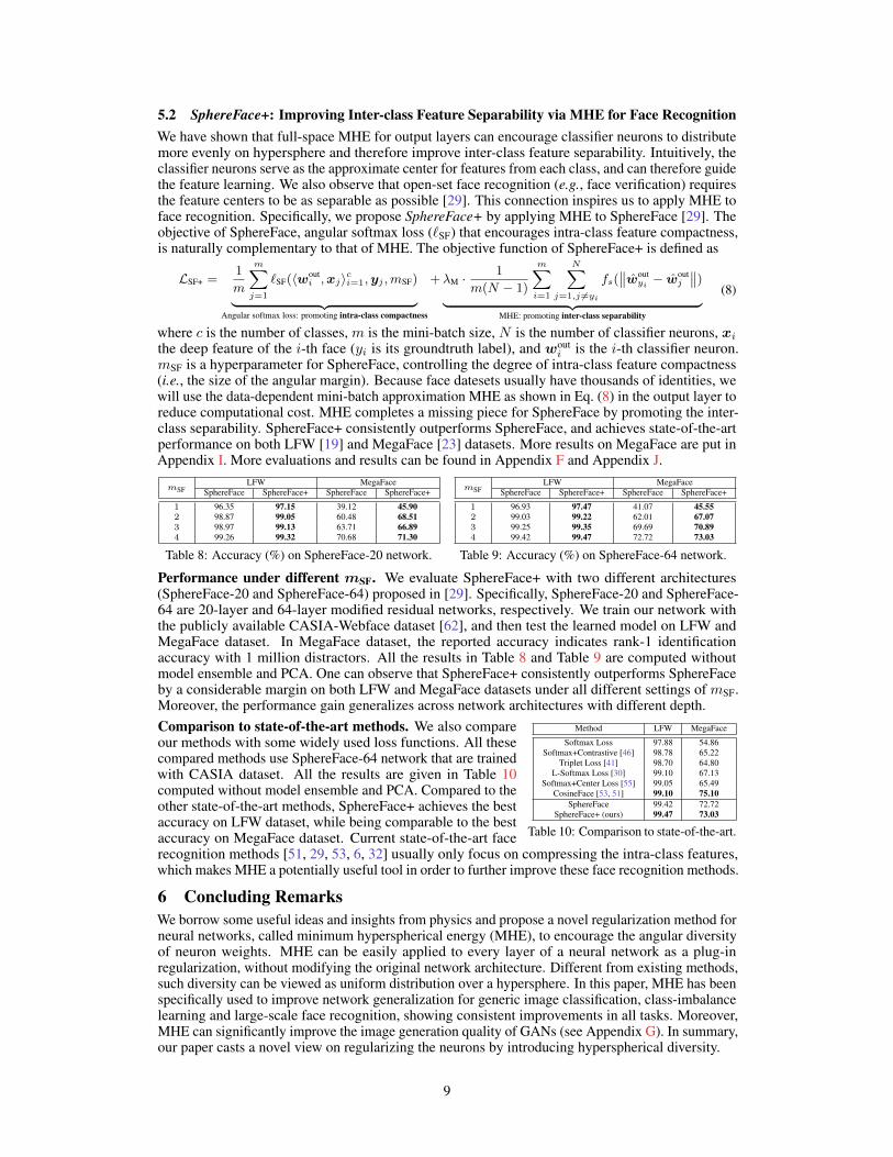
5.2 SphereFace+: Improving Inter-class Feature Separability via MHE for Face RecognitionWe have shown that full-space MHE for output layers can encourage classifier neurons to distributemore evenly on hypersphere and therefore improve inter-class feature separability. Intuitively, theclassifier neurons serve as the approximate center for features from each class, and can therefore guidethe feature learning. We also observe that open-set face recognition (e.g., face verification) requiresthe feature centers to be as separable as possible [29]. This connection inspires us to apply MHE toface recognition. Specifically, we propose SphereFace+ by applying MHE to SphereFace [29]. Theobjective of SphereFace, angular softmax loss (`SF) that encourages intra-class feature compactness,is naturally complementary to that of MHE. The objective function of SphereFace+ is defined as

LSF+ =1

m

m∑j=1

`SF(〈wouti ,xj〉ci=1,yj ,mSF)︸ ︷︷ ︸

Angular softmax loss: promoting intra-class compactness

+λM ·1

m(N − 1)

m∑i=1

N∑j=1,j 6=yi

fs(∥∥wout

yi − woutj

∥∥)︸ ︷︷ ︸MHE: promoting inter-class separability

(8)

where c is the number of classes, m is the mini-batch size, N is the number of classifier neurons, xithe deep feature of the i-th face (yi is its groundtruth label), and wout

i is the i-th classifier neuron.mSF is a hyperparameter for SphereFace, controlling the degree of intra-class feature compactness(i.e., the size of the angular margin). Because face datesets usually have thousands of identities, wewill use the data-dependent mini-batch approximation MHE as shown in Eq. (8) in the output layer toreduce computational cost. MHE completes a missing piece for SphereFace by promoting the inter-class separability. SphereFace+ consistently outperforms SphereFace, and achieves state-of-the-artperformance on both LFW [19] and MegaFace [23] datasets. More results on MegaFace are put inAppendix I. More evaluations and results can be found in Appendix F and Appendix J.

mSFLFW MegaFace

SphereFace SphereFace+ SphereFace SphereFace+

1 96.35 97.15 39.12 45.902 98.87 99.05 60.48 68.513 98.97 99.13 63.71 66.894 99.26 99.32 70.68 71.30

Table 8: Accuracy (%) on SphereFace-20 network.

mSFLFW MegaFace

SphereFace SphereFace+ SphereFace SphereFace+

1 96.93 97.47 41.07 45.552 99.03 99.22 62.01 67.073 99.25 99.35 69.69 70.894 99.42 99.47 72.72 73.03

Table 9: Accuracy (%) on SphereFace-64 network.

Performance under different mSF. We evaluate SphereFace+ with two different architectures(SphereFace-20 and SphereFace-64) proposed in [29]. Specifically, SphereFace-20 and SphereFace-64 are 20-layer and 64-layer modified residual networks, respectively. We train our network withthe publicly available CASIA-Webface dataset [62], and then test the learned model on LFW andMegaFace dataset. In MegaFace dataset, the reported accuracy indicates rank-1 identificationaccuracy with 1 million distractors. All the results in Table 8 and Table 9 are computed withoutmodel ensemble and PCA. One can observe that SphereFace+ consistently outperforms SphereFaceby a considerable margin on both LFW and MegaFace datasets under all different settings of mSF.Moreover, the performance gain generalizes across network architectures with different depth.

Method LFW MegaFace

Softmax Loss 97.88 54.86Softmax+Contrastive [46] 98.78 65.22

Triplet Loss [41] 98.70 64.80L-Softmax Loss [30] 99.10 67.13

Softmax+Center Loss [55] 99.05 65.49CosineFace [53, 51] 99.10 75.10

SphereFace 99.42 72.72SphereFace+ (ours) 99.47 73.03

Table 10: Comparison to state-of-the-art.

Comparison to state-of-the-art methods. We also compareour methods with some widely used loss functions. All thesecompared methods use SphereFace-64 network that are trainedwith CASIA dataset. All the results are given in Table 10computed without model ensemble and PCA. Compared to theother state-of-the-art methods, SphereFace+ achieves the bestaccuracy on LFW dataset, while being comparable to the bestaccuracy on MegaFace dataset. Current state-of-the-art facerecognition methods [51, 29, 53, 6, 32] usually only focus on compressing the intra-class features,which makes MHE a potentially useful tool in order to further improve these face recognition methods.

6 Concluding RemarksWe borrow some useful ideas and insights from physics and propose a novel regularization method forneural networks, called minimum hyperspherical energy (MHE), to encourage the angular diversityof neuron weights. MHE can be easily applied to every layer of a neural network as a plug-inregularization, without modifying the original network architecture. Different from existing methods,such diversity can be viewed as uniform distribution over a hypersphere. In this paper, MHE has beenspecifically used to improve network generalization for generic image classification, class-imbalancelearning and large-scale face recognition, showing consistent improvements in all tasks. Moreover,MHE can significantly improve the image generation quality of GANs (see Appendix G). In summary,our paper casts a novel view on regularizing the neurons by introducing hyperspherical diversity.

9

Acknowledgements

This project was supported in part by NSF IIS-1218749, NIH BIGDATA 1R01GM108341, NSFCAREER IIS-1350983, NSF IIS-1639792 EAGER, NSF IIS-1841351 EAGER, NSF CCF-1836822,NSF CNS-1704701, ONR N00014-15-1-2340, Intel ISTC, NVIDIA, Amazon AWS and Siemens.We would like to thank NVIDIA corporation for donating Titan Xp GPUs to support our research.We also thank Tuo Zhao for the valuable discussions and suggestions.

References[1] Alireza Aghasi, Nam Nguyen, and Justin Romberg. Net-trim: A layer-wise convex pruning of deep neural

networks. In NIPS, 2017. 1

[2] Jimmy Lei Ba, Jamie Ryan Kiros, and Geoffrey E Hinton. Layer normalization. arXiv preprintarXiv:1607.06450, 2016. 20

[3] Dmitriy Bilyk and Michael T Lacey. One-bit sensing, discrepancy and stolarsky’s principle. Sbornik:Mathematics, 208(6):744, 2017. 6

[4] Andrew Brock, Theodore Lim, James M Ritchie, and Nick Weston. Neural photo editing with introspectiveadversarial networks. In ICLR, 2017. 2, 20

[5] Michael Cogswell, Faruk Ahmed, Ross Girshick, Larry Zitnick, and Dhruv Batra. Reducing overfitting indeep networks by decorrelating representations. In ICLR, 2016. 1, 2

[6] Jiankang Deng, Jia Guo, and Stefanos Zafeiriou. Arcface: Additive angular margin loss for deep facerecognition. arXiv preprint arXiv:1801.07698, 2018. 9

[7] Ian Goodfellow, Jean Pouget-Abadie, Mehdi Mirza, Bing Xu, David Warde-Farley, Sherjil Ozair, AaronCourville, and Yoshua Bengio. Generative adversarial nets. In NIPS, 2014. 20

[8] Mario Götz and Edward B Saff. Note on d—extremal configurations for the sphere in r d+1. In RecentProgress in Multivariate Approximation, pages 159–162. Springer, 2001. 5, 15

[9] Ishaan Gulrajani, Faruk Ahmed, Martin Arjovsky, Vincent Dumoulin, and Aaron C Courville. Improvedtraining of wasserstein gans. In NIPS, 2017. 20

[10] Yandong Guo, Lei Zhang, Yuxiao Hu, Xiaodong He, and Jianfeng Gao. Ms-celeb-1m: A dataset andbenchmark for large-scale face recognition. In ECCV, 2016. 25

[11] Song Han, Huizi Mao, and William J Dally. Deep compression: Compressing deep neural networks withpruning, trained quantization and huffman coding. In ICLR, 2016. 1

[12] DP Hardin and EB Saff. Minimal riesz energy point configurations for rectifiable d-dimensional manifolds.arXiv preprint math-ph/0311024, 2003. 5, 15

[13] DP Hardin and EB Saff. Discretizing manifolds via minimum energy points. Notices of the AMS,51(10):1186–1194, 2004. 5, 6

[14] Kaiming He, Xiangyu Zhang, Shaoqing Ren, and Jian Sun. Delving deep into rectifiers: Surpassinghuman-level performance on imagenet classification. In ICCV, 2015. 6

[15] Kaiming He, Xiangyu Zhang, Shaoqing Ren, and Jian Sun. Deep residual learning for image recognition.In CVPR, 2016. 1, 6, 8, 13

[16] Kaiming He, Xiangyu Zhang, Shaoqing Ren, and Jian Sun. Identity mappings in deep residual networks.In ECCV, 2016. 8

[17] Andrew G Howard, Menglong Zhu, Bo Chen, Dmitry Kalenichenko, Weijun Wang, Tobias Weyand, MarcoAndreetto, and Hartwig Adam. Mobilenets: Efficient convolutional neural networks for mobile visionapplications. arXiv preprint arXiv:1704.04861, 2017. 1

[18] Gao Huang, Zhuang Liu, Laurens Van Der Maaten, and Kilian Q Weinberger. Densely connectedconvolutional networks. In CVPR, 2017. 8

[19] Gary B Huang, Manu Ramesh, Tamara Berg, and Erik Learned-Miller. Labeled faces in the wild: Adatabase for studying face recognition in unconstrained environments. Technical report, Technical Report,2007. 9

10

[20] Forrest N Iandola, Song Han, Matthew W Moskewicz, Khalid Ashraf, William J Dally, and Kurt Keutzer.Squeezenet: Alexnet-level accuracy with 50x fewer parameters and< 0.5 mb model size. arXiv preprintarXiv:1602.07360, 2016. 1

[21] Sergey Ioffe and Christian Szegedy. Batch normalization: Accelerating deep network training by reducinginternal covariate shift. In ICML, 2015. 2, 6, 20

[22] Lu Jiang, Deyu Meng, Shoou-I Yu, Zhenzhong Lan, Shiguang Shan, and Alexander Hauptmann. Self-pacedlearning with diversity. In NIPS, 2014. 2

[23] Ira Kemelmacher-Shlizerman, Steven M Seitz, Daniel Miller, and Evan Brossard. The megaface benchmark:1 million faces for recognition at scale. In CVPR, 2016. 9

[24] Arno Kuijlaars and E Saff. Asymptotics for minimal discrete energy on the sphere. Transactions of theAmerican Mathematical Society, 350(2):523–538, 1998. 5, 6, 15

[25] Ludmila I Kuncheva and Christopher J Whitaker. Measures of diversity in classifier ensembles and theirrelationship with the ensemble accuracy. Machine learning, 51(2):181–207, 2003. 2

[26] Naum Samouilovich Landkof. Foundations of modern potential theory, volume 180. Springer, 1972. 5, 15

[27] Nan Li, Yang Yu, and Zhi-Hua Zhou. Diversity regularized ensemble pruning. In Joint EuropeanConference on Machine Learning and Knowledge Discovery in Databases, 2012. 2

[28] Weiyang Liu, Zhen Liu, Zhiding Yu, Bo Dai, Rongmei Lin, Yisen Wang, James M Rehg, and Le Song.Decoupled networks. CVPR, 2018. 1, 5, 6, 16

[29] Weiyang Liu, Yandong Wen, Zhiding Yu, Ming Li, Bhiksha Raj, and Le Song. Sphereface: Deephypersphere embedding for face recognition. In CVPR, 2017. 1, 2, 5, 9, 14, 19, 25

[30] Weiyang Liu, Yandong Wen, Zhiding Yu, and Meng Yang. Large-margin softmax loss for convolutionalneural networks. In ICML, 2016. 1, 2, 4, 9, 22

[31] Weiyang Liu, Yan-Ming Zhang, Xingguo Li, Zhiding Yu, Bo Dai, Tuo Zhao, and Le Song. Deephyperspherical learning. In NIPS, 2017. 1, 2, 4, 5, 6, 8, 16, 18

[32] Yu Liu, Hongyang Li, and Xiaogang Wang. Rethinking feature discrimination and polymerization forlarge-scale recognition. arXiv preprint arXiv:1710.00870, 2017. 9

[33] Julien Mairal, Francis Bach, Jean Ponce, and Guillermo Sapiro. Online dictionary learning for sparsecoding. In ICML, 2009. 2

[34] Dmytro Mishkin and Jiri Matas. All you need is a good init. In ICLR, 2016. 2

[35] Takeru Miyato, Toshiki Kataoka, Masanori Koyama, and Yuichi Yoshida. Spectral normalization forgenerative adversarial networks. In ICLR, 2018. 2, 20

[36] Ignacio Ramirez, Pablo Sprechmann, and Guillermo Sapiro. Classification and clustering via dictionarylearning with structured incoherence and shared features. In CVPR, 2010. 2

[37] Pau Rodríguez, Jordi Gonzalez, Guillem Cucurull, Josep M Gonfaus, and Xavier Roca. Regularizing cnnswith locally constrained decorrelations. In ICLR, 2017. 1, 2, 5, 8

[38] Aruni RoyChowdhury, Prakhar Sharma, Erik Learned-Miller, and Aruni Roy. Reducing duplicate filters indeep neural networks. In NIPS workshop on Deep Learning: Bridging Theory and Practice, 2017. 1

[39] Edward B Saff and Amo BJ Kuijlaars. Distributing many points on a sphere. The mathematical intelligencer,19(1):5–11, 1997. 5, 6

[40] Tim Salimans and Diederik P Kingma. Weight normalization: A simple reparameterization to acceleratetraining of deep neural networks. In NIPS, 2016. 20

[41] Florian Schroff, Dmitry Kalenichenko, and James Philbin. Facenet: A unified embedding for facerecognition and clustering. In CVPR, 2015. 9

[42] Wenling Shang, Kihyuk Sohn, Diogo Almeida, and Honglak Lee. Understanding and improving convolu-tional neural networks via concatenated rectified linear units. In ICML, 2016. 1

[43] Karen Simonyan and Andrew Zisserman. Very deep convolutional networks for large-scale image recogni-tion. arXiv:1409.1556, 2014. 1

11

[44] Steve Smale. Mathematical problems for the next century. The mathematical intelligencer, 20(2):7–15,1998. 2, 5

[45] Nitish Srivastava, Geoffrey Hinton, Alex Krizhevsky, Ilya Sutskever, and Ruslan Salakhutdinov. Dropout:A simple way to prevent neural networks from overfitting. JMLR, 15(1):1929–1958, 2014. 2

[46] Yi Sun, Xiaogang Wang, and Xiaoou Tang. Deep learning face representation from predicting 10,000classes. In CVPR, 2014. 9

[47] Christian Szegedy, Wei Liu, Yangqing Jia, Pierre Sermanet, Scott Reed, Dragomir Anguelov, DumitruErhan, Vincent Vanhoucke, and Andrew Rabinovich. Going deeper with convolutions. In CVPR, 2015. 1,8

[48] Pieter Merkus Lambertus Tammes. On the origin of number and arrangement of the places of exit on thesurface of pollen-grains. Recueil des travaux botaniques néerlandais, 27(1):1–84, 1930. 5

[49] Joseph John Thomson. Xxiv. on the structure of the atom: an investigation of the stability and periodsof oscillation of a number of corpuscles arranged at equal intervals around the circumference of a circle;with application of the results to the theory of atomic structure. The London, Edinburgh, and DublinPhilosophical Magazine and Journal of Science, 7(39):237–265, 1904. 2, 5

[50] Fei Wang, Liren Chen, Cheng Li, Shiyao Huang, Yanjie Chen, Chen Qian, and Chen Change Loy. Thedevil of face recognition is in the noise. In ECCV, 2018. 25

[51] Feng Wang, Weiyang Liu, Haijun Liu, and Jian Cheng. Additive margin softmax for face verification.arXiv preprint arXiv:1801.05599, 2018. 9, 19

[52] Feng Wang, Xiang Xiang, Jian Cheng, and Alan L Yuille. Normface: L2 hypersphere embedding for faceverification. arXiv preprint arXiv:1704.06369, 2017. 19

[53] Hao Wang, Yitong Wang, Zheng Zhou, Xing Ji, Zhifeng Li, Dihong Gong, Jingchao Zhou, and Wei Liu.Cosface: Large margin cosine loss for deep face recognition. arXiv preprint arXiv:1801.09414, 2018. 9, 14

[54] David Warde-Farley and Yoshua Bengio. Improving generative adversarial networks with denoising featurematching. In ICLR, 2017. 20

[55] Yandong Wen, Kaipeng Zhang, Zhifeng Li, and Yu Qiao. A discriminative feature learning approach fordeep face recognition. In ECCV, 2016. 9

[56] Bo Xie, Yingyu Liang, and Le Song. Diverse neural network learns true target functions. arXiv preprintarXiv:1611.03131, 2016. 5, 6

[57] Di Xie, Jiang Xiong, and Shiliang Pu. All you need is beyond a good init: Exploring better solution for train-ing extremely deep convolutional neural networks with orthonormality and modulation. arXiv:1703.01827,2017. 2

[58] Pengtao Xie, Yuntian Deng, Yi Zhou, Abhimanu Kumar, Yaoliang Yu, James Zou, and Eric P Xing.Learning latent space models with angular constraints. In ICML, 2017. 1, 2, 5

[59] Pengtao Xie, Aarti Singh, and Eric P Xing. Uncorrelation and evenness: a new diversity-promotingregularizer. In ICML, 2017. 1, 2

[60] Pengtao Xie, Wei Wu, Yichen Zhu, and Eric P Xing. Orthogonality-promoting distance metric learning:convex relaxation and theoretical analysis. In ICML, 2018. 2

[61] Pengtao Xie, Jun Zhu, and Eric Xing. Diversity-promoting bayesian learning of latent variable models. InICML, 2016. 1, 2

[62] Dong Yi, Zhen Lei, Shengcai Liao, and Stan Z Li. Learning face representation from scratch.arXiv:1411.7923, 2014. 9

[63] Kaipeng Zhang, Zhanpeng Zhang, Zhifeng Li, and Yu Qiao. Joint face detection and alignment usingmultitask cascaded convolutional networks. IEEE Signal Processing Letters, 23(10):1499–1503, 2016. 14

[64] Xiangyu Zhang, Xinyu Zhou, Mengxiao Lin, and Jian Sun. Shufflenet: An extremely efficient convolutionalneural network for mobile devices. arXiv preprint arXiv:1707.01083, 2017. 1

12

AppendixA Experimental Details

Layer CNN-6 CNN-9 CNN-15

Conv1.x [3×3, 64]×2 [3×3, 64]×3 [3×3, 64]×5Pool1 2×2 Max Pooling, Stride 2

Conv2.x [3×3, 128]×2 [3×3, 128]×3 [3×3, 128]×5Pool2 2×2 Max Pooling, Stride 2

Conv3.x [3×3, 256]×2 [3×3, 256]×3 [3×3, 256]×5Pool3 2×2 Max Pooling, Stride 2

Fully Connected 256 256 256

Table 11: Our plain CNN architectures with different convolutional layers. Conv1.x, Conv2.x and Conv3.xdenote convolution units that may contain multiple convolution layers. E.g., [3×3, 64]×3 denotes 3 cascadedconvolution layers with 64 filters of size 3×3.

Layer ResNet-32 for CIFAR-10/100 ResNet-18 for ImageNet-2012 ResNet-34 for ImageNet-2012

Conv0.x N/A [7×7, 64], Stride 23×3, Max Pooling, Stride 2

[7×7, 64], Stride 23×3, Max Pooling, Stride 2

Conv1.x

[3×3, 64]×1[3× 3, 64

3× 3, 64

]× 5

[3× 3, 64

3× 3, 64

]× 2

[3× 3, 64

3× 3, 64

]× 3

Conv2.x

[3× 3, 128

3× 3, 128

]× 5

[3× 3, 128

3× 3, 128

]× 2

[3× 3, 128

3× 3, 128

]× 4

Conv3.x

[3× 3, 256

3× 3, 256

]× 5

[3× 3, 256

3× 3, 256

]× 2

[3× 3, 256

3× 3, 256

]× 6

Conv4.x N/A

[3× 3, 512

3× 3, 512

]× 2

[3× 3, 512

3× 3, 512

]× 3

Average Pooling

Table 12: Our ResNet architectures with different convolutional layers. Conv0.x, Conv1.x, Conv2.x, Conv3.xand Conv4.x denote convolution units that may contain multiple convolutional layers, and residual units areshown in double-column brackets. Conv1.x, Conv2.x and Conv3.x usually operate on different size featuremaps. These networks are essentially the same as [15], but some may have a different number of filters in eachlayer. The downsampling is performed by convolutions with a stride of 2. E.g., [3×3, 64]×4 denotes 4 cascadedconvolution layers with 64 filters of size 3×3, and S2 denotes stride 2.

General settings. The network architectures used in the paper are elaborated in Table 11 Table 12.For CIFAR-10 and CIFAR-100, we use batch size 128. We start with learning rate 0.1, divide it by 10at 20k, 30k and 37.5k iterations, and terminate training at 42.5k iterations. For ImageNet-2012, weuse batch size 64 and start with learning rate 0.1. The learning rate is divided by 10 at 150k, 300kand 400k iterations, and the training is terminated at 500k iterations. Note that, for all the comparedmethods, we always use the best possible hyperparameters to make sure that the comparison is fair.The baseline has exactly the same architecture and training settings as the one that MHE uses, andthe only difference is an additional MHE regularization. For full-space MHE in hidden layers, we setλh as 10 for all experiments. For half-space MHE in hidden layers, we set λh as 1 for all experiments.For MHE in output layers, we set λo as 1 for all experiments. We use 1e−5 for the orthonormalregularization. If not otherwise specified, standard `2 weight decay (1e−4) is applied to all the neuralnetwork including baselines and the networks that use MHE regularization. A very minor issue forthe hyperparameters λh is that it may increase as the number of layers increases, so we can potentiallyfurther divide the hyperspherical energy for the hidden layers by the number of layers. It will probablychange the current optimal hyperparameter setting by a constant multiplier. For notation simplicity,we do not explicitly write out the weight decay term in the loss function in the main paper. Note that,all the neuron weights in the neural networks used in the paper are not normalized (unless otherwisespecified), but the MHE will normalize the neuron weights while computing the regularization loss.As a result, MHE does not need to modify any component of the original neural networks, and it cansimply be viewed as an extra regularization loss that can boost the performance. Because half-spacevariants can only applied to the hidden layers, both original MHE and its half-space version apply thefull-space MHE to the output layer by default. The difference between MHE and half-space MHEare only in the regularization for the hidden layers.Class-imbalance learning. There are 50000 training images in the original CIFAR-10 dataset, with5000 images per class. For the single class imbalance setting, we keep original images of class

13

1-9 and randomly throw away 90% images of class 0. The total number of training images in thissetting is 45500. For the multiple class imbalance setting, we set the number of each class equalsto 500×(class_index+1). For instance, class 0 has 500 images, class 1 has 1000 images and class9 has 5000 images. The total number of training images in this setting is 27500. Note that, bothhalf-space MHE and half-space A-MHE in Table 7 and Table 8 mean that the half-space variantshave been applied to the hidden layers. For the output layer (i.e., classifier neurons), only full-spaceMHE can be used.SphereFace+. SphereFace+ uses the same face detection and alignment method [63] asSphereFace [29]. The testing protocol on LFW and MegaFace is also the same as SphereFace.We use exactly the same preprocessing as in the SphereFace repository. Detailed network archi-tecture settings of SphereFace-20 and SphereFace-64 can be found in [29]. Specifically, we usefull-space MHE with Euclidean distance and s = 2 in the output layer. Essentially, we treat MHEas an additional loss function which aims to enlarge the inter-class angular distance of features andserves a complementary role to the angular softmax in SphereFace. Note that, for the results ofCosineFace [53], we directly use the results (with the same training settings and without using featurenormalization) reported in the paper. Since ours also does not perform feature normalization, it is afair comparison. With feature normalization, we find that the performance of SphereFace+ will alsobe improved significantly. However, feature normalization makes the results more tricky, because itwill involve another hyperparameter that controls the projection radius of feature normalization.

In order to reduce the training difficulty, we adopt a new training strategy. Specifically, we first train amodel using the original SphereFace, and then use the new loss function proposed in Eq. 8 to finetunethe pretrained SphereFace model. Note that, only the results for face recognition are obtained usingthis training strategy.

14

B Proof of Theorem 1 and Theorem 2

Theorem 1 and Theorem 2 are natural results from classic potential theory [26] and sphericalconfiguration [12, 24, 8]. We discuss the asymptotic behavior (N→∞) in three cases: 0<s<d,s=d, and s>d. We first write the energy integral as

Is(µ) =

∫∫Sd×Sd

‖u− v‖−sdµ(u)dµ(v), (9)

which is taken over all probability measure µ supported on Sd. With 0<s<d, Is(µ) is minimal whenµ is the spherical measure σd=Hd(·)|Sd/Hd(Sd) on Sd, where Hd(·) denotes the d-dimensionalHausdorff measure. When s≥d, Is(µ) becomes infinity, which therefore requires different analysis.

First, the classic potential theory [26] can directly give the following results for the case where0 < s < d:Lemma 1. If 0 < s < d,

limN→∞

εs,d(N)

N2= Is(

Hd(·)|SdHd(Sd)

), (10)

where Is is defined in the main paper. Moreover, any sequence of optimal hyperspherical s-enerygyconfigurations (W ?

N )|∞2 ⊂Sd is asymptotically uniformly distributed in the sense that for the weak-star topology measures,

1

N

∑v∈W ?

N

δv → σd, as N →∞ (11)

where δv denotes the unit point mass at v, and σd is the spherical measure on Sd.

which directly concludes Theorem 1 and Theorem 2 in the case of 0 < s < d.

For the case where s = d, we have from [24, 8] the following results:Lemma 2. Let Bd := B(0, 1) be the closed unit ball in Rd. For s = d,

limN→∞

εs,d(N)

N2 logN=Hd(Bd)Hd(Sd)

=1

d

Γ(d+12 )

√πΓ(d2 )

, (12)

and any sequence (W ?N )|∞2 ⊂Sd of optimal s-energy configurations satisfies Eq. 11.

which concludes the case of s = d. Therefore, we are left with the case where s > d. For this case,we can use the results from [12]:Lemma 3. Let A ⊂ Rd be compact with Hd(A) > 0, and WN = {xk,N}Ni=1 be a sequence ofasymptotically optimal N -point configurations in A in the sense that for some s > d,

limN→∞

Es(WN )

N1+s/d=

Cs,dHd(A)s/d

(13)

or

limN→∞

Es(WN )

N2 logN=Hd(Bd)Hd(A)

. (14)

where Cs,d is a finite positive constant independent of A. Let δx be the unit point mass at the point x.Then in the weak-star topology of measures we have

1

N

N∑i=1

δxi,N→ H

d(·)|AHd(A)

, asN →∞. (15)

The results naturally prove the case of s > d. Combining these three lemmas, we have provedTheorem 1 and Theorem 2.

15

C Understanding MHE from Decoupled View

Inspired by decoupled networks [28], we can view the original convolution as the multiplication ofthe angular function g(θ)=cos(θ) and the magnitude function h(‖w‖ , ‖x‖)=‖w‖·‖x‖:

f(w,x) = h(‖w‖ , ‖x‖) · g(θ)

=(‖w‖ · ‖x‖

)·(

cos(θ)) (16)

where θ is the angle between the kernel w and the input x. From the equation above, we can see thatthe norm of the kernel and the direction (i.e., angle) of the kernel affect the inner product similaritydifferently. Typically, weight decay is to regularize the kernel by minimizing its `2 norm, whilethere is no regularization on the direction of the kernel. Therefore, MHE is able to complete thismissing piece by promoting angular diversity. By combining MHE to a standard neural networks(e.g., CNNs), the regularization term becomes

Lreg = λw ·1∑L

j=1Nj

L∑j=1

Nj∑i=1

‖wi‖︸ ︷︷ ︸Weight decay: regularizing the magnitude of kernels

+λh ·L−1∑j=1

1

Nj(Nj − 1){Es}j + λo ·

1

NL(NL − 1)Es(w

outi |ci=1)︸ ︷︷ ︸

MHE: regularizing the direction of kernels

(17)where xi is the feature of the i-th training sample entering the output layer, wout

i is the classifierneuron for the i-th class in the output fully-connected layer and wout

i denotes its normalized version.{Es}i denotes the hyperspherical energy for the neurons in the i-th layer. c is the number of classes,m is the batch size, L is the number of layers of the neural network, and Ni is the number of neuronsin the i-th layer. Es(w

outi |ci=1) denotes the hyperspherical energy of neurons {wout

1 , · · · , woutc } in the

output layer. λw, λh and λo are weighting hyperparameters for these three regularization terms.

From the decoupled view, we can see that MHE is actually very meaningful in regularizing the neuralnetworks, and it also serves as a complementary role to weight decay. According to [28] (usingclassifier neurons as an intuitive example), weight decay is used to regularize the intra-class variation,while MHE is used to regularize the inter-class semantic difference. In such sense, MHE completesan important missing piece for the standard neural networks by regularizing the directions of neurons(i.e., kernels). In contrast, the standard neural networks only have weight decay as a regularizationfor the norm of neurons.

Weight decay can help to prevent the network from overfitting and improve the generalization.Similarly, MHE can serve as a similar role, and we argue that MHE is very likely to be more crucialthan weight decay in avoiding overfitting and improving generalization. Our intuition comes fromSphereNets [31] which shows that the magnitude of kernels is not important for object recognition.Therefore, the directions of the kernels are directly related to the semantic discrimination of the neuralnetworks, and MHE is designed to regularize the directions of kernels by imposing the hypersphericaldiversity. To conclude, MHE provides a novel hyperspherical perspective for regularizing neuralnetworks.

16

D Weighted MHE

In this section, we do a preliminary study for weighted MHE. To be clear, weighted MHE is tocompute MHE with neurons with different fixed weights. Taking Euclidean distance MHE as anexample, weighted MHE can be formulated as:

Es,d(βiwi|Ni=1) =

N∑i=1

N∑j=1,j 6=i

fs(‖βiwi − βjwj‖

)=

{ ∑i6=j ‖βiwi − βjwj‖−s , s > 0∑i6=j log

(‖βiwi − βjwj‖−1 ), s = 0

,

(18)where βi is a constant weight for the neuron wi. We perform a toy experiment to see how theseweights βi can affect the neuron distribution on 3-dimensional sphere. Specifically, we follow thesame setting as Fig. 1, and apply weighted MHE to 10 normalized vectors in 3-dimensional space.We experiment two settings: (1) only one neuron w1 has different weight β1 than the other 9 neurons;(2) two neurons w1,w2 have different weight β1, β2 than the other 8 neurons. For the first setting,we visualize the cases where β1 = 1, 2, 4, 10 and βi = 1, 10 ≥ i ≥ 2. The visualization results areshown in Fig. 5. For the second setting, we visualize the cases where β1 = β2 = 1, 2, 4, 10 andβi = 1, 10 ≥ i ≥ 3. The visualization results are shown in Fig. 6. In these visualization experiments,we only use the gradient of weighted MHE to update the randomly initialized neurons. Note that, forall experiments, the random seed is fixed.

(a) β1=1 (b) β1=2 (c) β1=4 (d) β1=10

Figure 5: The visualization of normalized neurons after applying weighted MHE in the first setting. Theblue-green square dots denote the trajectory (history of the iterates) of neuron w1 with β1 = 1, 2, 4, 10, whilethe red dots denote the neurons with βi = 1, i 6= 1. The final neuron w1 is connected to the origin with a solidblue line. The dash line is used to connected the trajectory.

(a) β1=β2=1 (b) β1=β2=2 (c) β1=β2=4 (d) β1=β2=10

Figure 6: The visualization of normalized neurons after applying weighted MHE in the second setting. The blue-green square dots denote the trajectory of neuron w1 with β1 = 1, 2, 4, 10, the pure green square dots denote thetrajectory of neuron w2 with β2 = 1, 2, 4, 10, and the red dots denote the neurons with βi = 1, i 6= 1, 2. Thefinal neurons w1 and w2 are connected to the origin with a solid blue line and a solid green line, respectively.The dash line is used to connected the trajectory.

From both Fig. 5 and Fig. 6, one can observe that the neurons with larger β tend to be more “fixed”(unlikely to move), and the neurons with smaller β tend to move more flexibly. This can also beinterpreted as the neurons with larger β being more important. Such phenomena indicate that wecan control the flexibility of the neurons under the learning dynamics of MHE. There is one scenariowhere weighted MHE may be very useful. Suppose we have known that some neurons are alreadywell learned (e.g., some filters from a pretrained model) and we do not want these neurons to beupdated dramatically, then we can use the weighted MHE and set a larger β for these neurons.

17

E Regularizing SphereNets with MHE

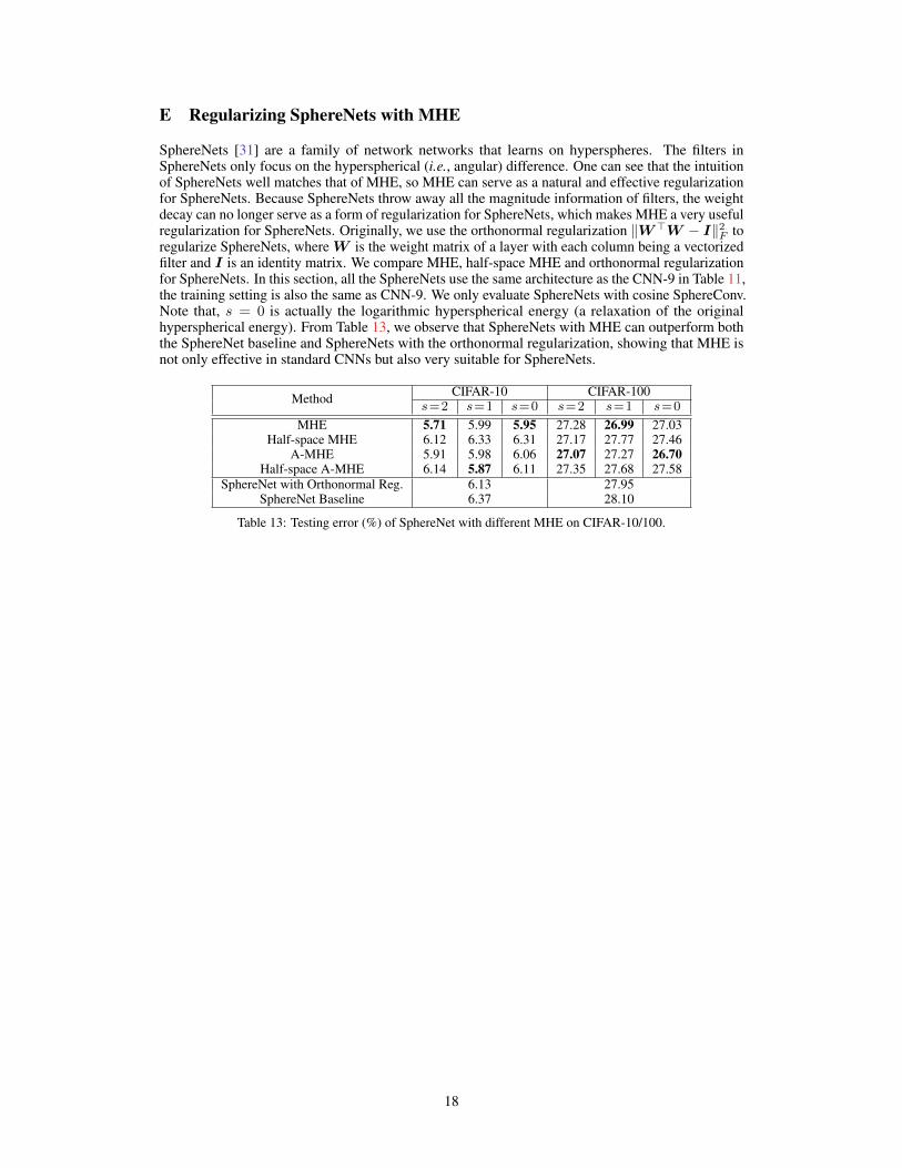
SphereNets [31] are a family of network networks that learns on hyperspheres. The filters inSphereNets only focus on the hyperspherical (i.e., angular) difference. One can see that the intuitionof SphereNets well matches that of MHE, so MHE can serve as a natural and effective regularizationfor SphereNets. Because SphereNets throw away all the magnitude information of filters, the weightdecay can no longer serve as a form of regularization for SphereNets, which makes MHE a very usefulregularization for SphereNets. Originally, we use the orthonormal regularization ‖W>W − I‖2F toregularize SphereNets, where W is the weight matrix of a layer with each column being a vectorizedfilter and I is an identity matrix. We compare MHE, half-space MHE and orthonormal regularizationfor SphereNets. In this section, all the SphereNets use the same architecture as the CNN-9 in Table 11,the training setting is also the same as CNN-9. We only evaluate SphereNets with cosine SphereConv.Note that, s = 0 is actually the logarithmic hyperspherical energy (a relaxation of the originalhyperspherical energy). From Table 13, we observe that SphereNets with MHE can outperform boththe SphereNet baseline and SphereNets with the orthonormal regularization, showing that MHE isnot only effective in standard CNNs but also very suitable for SphereNets.

Method CIFAR-10 CIFAR-100s=2 s=1 s=0 s=2 s=1 s=0

MHE 5.71 5.99 5.95 27.28 26.99 27.03Half-space MHE 6.12 6.33 6.31 27.17 27.77 27.46

A-MHE 5.91 5.98 6.06 27.07 27.27 26.70Half-space A-MHE 6.14 5.87 6.11 27.35 27.68 27.58

SphereNet with Orthonormal Reg. 6.13 27.95SphereNet Baseline 6.37 28.10

Table 13: Testing error (%) of SphereNet with different MHE on CIFAR-10/100.

18

F Improving AM-Softmax with MHE

We also perform some preliminary experiments for applying MHE to additive margin softmaxloss [51] which is a recently proposed well-performing objective function for face recognition. Theloss function of AM-Softmax is given as follows:

LAMS = − 1

n

n∑i=1

loges·(cosθ(xi,wyi

)−mAMS

)

es·(cosθ(xi,wyi

)−mAMS

)+∑cj=1,j 6=yi e

s·cosθ(xi,wj)

(19)

where yi is the label of the training sample xi, n is the mini-batch size, mAMS is the hyperparameterthat controls the degree of angular margin, and θ(xi,wj) denotes the angle between the training samplexi and the classifier neuron wj . s is the hyperparameter that controls the projection radius of featurenormalization [52, 51]. Similar to our SphereFace+, we combine full-space MHE to the outputlayer to improve the inter-class feature separability. It is essentially following the same intuition ofSphereFace+ by adding an additional loss function to AM-Softmax loss.

Experiments. We perform a preliminary experiment to study the benefits of MHE for improving AM-Softmax loss. We use the SphereFace-20 network and trained on CASIA-WebFace dataset (trainingsettings are exactly the same as SphereFace+ in the main paper and [29]). The hyperparameterss,mAMS for AM-Softmax loss exactly follow the best setting in [51]. AM-Softmax achieves 99.26%accuracy on LFW, while combining MHE with AM-Softmax yields 99.37% accuracy on LFW.Such performance gain is actually very significant in face verification, which further validates thesuperiority of MHE.

19

G Improving GANs with MHE

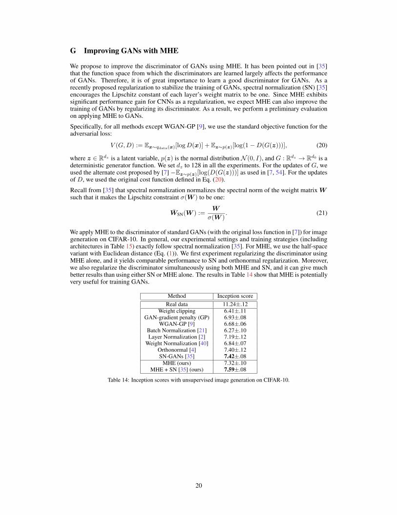
We propose to improve the discriminator of GANs using MHE. It has been pointed out in [35]that the function space from which the discriminators are learned largely affects the performanceof GANs. Therefore, it is of great importance to learn a good discriminator for GANs. As arecently proposed regularization to stabilize the training of GANs, spectral normalization (SN) [35]encourages the Lipschitz constant of each layer’s weight matrix to be one. Since MHE exhibitssignificant performance gain for CNNs as a regularization, we expect MHE can also improve thetraining of GANs by regularizing its discriminator. As a result, we perform a preliminary evaluationon applying MHE to GANs.

Specifically, for all methods except WGAN-GP [9], we use the standard objective function for theadversarial loss:

V (G,D) := Ex∼qdata(x)[logD(x)] + Ez∼p(z)[log(1−D(G(z)))], (20)

where z ∈ Rdz is a latent variable, p(z) is the normal distribution N (0, I), and G : Rdz → Rd0 is adeterministic generator function. We set dz to 128 in all the experiments. For the updates of G, weused the alternate cost proposed by [7] −Ez∼p(z)[log(D(G(z)))] as used in [7, 54]. For the updatesof D, we used the original cost function defined in Eq. (20).

Recall from [35] that spectral normalization normalizes the spectral norm of the weight matrix Wsuch that it makes the Lipschitz constraint σ(W ) to be one:

WSN(W ) :=W

σ(W ). (21)

We apply MHE to the discriminator of standard GANs (with the original loss function in [7]) for imagegeneration on CIFAR-10. In general, our experimental settings and training strategies (includingarchitectures in Table 15) exactly follow spectral normalization [35]. For MHE, we use the half-spacevariant with Euclidean distance (Eq. (1)). We first experiment regularizing the discriminator usingMHE alone, and it yields comparable performance to SN and orthonormal regularization. Moreover,we also regularize the discriminator simultaneously using both MHE and SN, and it can give muchbetter results than using either SN or MHE alone. The results in Table 14 show that MHE is potentiallyvery useful for training GANs.

Method Inception scoreReal data 11.24±.12

Weight clipping 6.41±.11GAN-gradient penalty (GP) 6.93±.08

WGAN-GP [9] 6.68±.06Batch Normalization [21] 6.27±.10Layer Normalization [2] 7.19±.12

Weight Normalization [40] 6.84±.07Orthonormal [4] 7.40±.12SN-GANs [35] 7.42±.08

MHE (ours) 7.32±.10MHE + SN [35] (ours) 7.59±.08

Table 14: Inception scores with unsupervised image generation on CIFAR-10.

20

G.1 Network Architecture for GAN

We give the detailed network architectures in Table 15 that are used in our experiments for thegenerator and the discriminator.

Table 15: Our CNN architectures for image Generation on CIFAR-10. The slopes of all leaky ReLU (lReLU)functions in the networks are set to 0.1.

z ∈ R128 ∼ N (0, I)dense→Mg ×Mg × 512

4×4, stride=2 deconv. BN 256 ReLU4×4, stride=2 deconv. BN 128 ReLU4×4, stride=2 deconv. BN 64 ReLU

3×3, stride=1 conv. 3 Tanh

(a) Generator (Mg = 4 for CIFAR10).

RGB image x ∈ RM×M×3

3×3, stride=1 conv 64 lReLU4×4, stride=2 conv 64 lReLU

3×3, stride=1 conv 128 lReLU4×4, stride=2 conv 128 lReLU3×3, stride=1 conv 256 lReLU4×4, stride=2 conv 256 lReLU3×3, stride=1 conv. 512 lReLU

dense→ 1

(b) Discriminator (M = 32 CIFAR10).

G.2 Comparison of Random Generated Images

We provide some randomly generated images for comparison between baseline GAN and GANregularized by both MHE and SN. The generated images are shown in Fig. 7.

Baseline GAN GAN with MHE and SNDatasetFigure 7: Results of generated images.

21

H More Results on Class-imbalance Learning

H.1 Class-imbalance learning on CIFAR-100

We perform additional experiments on CIFAR-100 to further validate the effectiveness of MHE inclass-imbalance learning. In the CNN used in the experiment, we only apply MHE (i.e., full-spaceMHE) to the output layer, and use MHE or half-space MHE in the hidden layers. In general, theexperimental settings are the same as the main paper. We still use CNN-9 (which is a 9-layer CNNfrom Table 11) in the experiment. Slightly differently from CIFAR-10 in the main paper, the twodata imbalance settings on CIFAR-100 include 1) 10-class imbalance (denoted as Single in Table 16)- All classes have the same number of images but 10 classes (index from 0 to 9) have significantlyless number (only 10% training samples compared to the other normal classes), and 2) multiple classimbalance (denoted by Multiple in Table 16) - The number of images decreases as the class indexdecreases from 99 to 0. For the multiple class imbalance setting, we set the number of each classequals to 5×(class_index+1). Experiment details are similar to the CIFAR-10 experiment, whichis specified in Appendix A. The results in Table 16 show that MHE consistently improves CNNsin class-imbalance learning on CIFAR-100. In most cases, half-space MHE performs better thanfull-space MHE.

Method Single MultipleBaseline 31.43 38.39

Orthonormal 30.75 37.89MHE 29.30 37.07

Half-space MHE 29.40 36.52A-MHE 30.16 37.54

Half-space A-MHE 29.60 37.07

Table 16: Error rate (%) on imbalanced CIFAR-100.

H.2 2D CNN Feature Visualization

(a) CNN without MHE (Training Set) (b) CNN with MHE (Training Set)

(c) CNN without MHE (Testing Set) (d) CNN features with MHE (Testing Set)

Figure 8: 2D CNN features with or without MHE on both training set and testing set. The features are computedby setting the output feature dimension as 2, similar to [30]. Each point denotes the 2D feature of a data point,and each color denotes a class. The red arrows are the classifier neurons of the output layer.

22

The experimental settings are the same as the main paper. We supplement the 2D feature visualizationon testing set in Fig. 8. The visualized features on both training set and testing set well demonstratethe superiority of MHE in class-imbalance learning. In the CNN without MHE, the classifier neuronof the imbalanced training data is highly biased towards another class, and therefore can not beproperly learned. In contrast, the CNN with MHE can learn uniformly distributed classifier neurons,which greatly improves the network’s generalization ability.

23

I More results of SphereFace+ on Megaface Challenge

We give more experimental results of SphereFace+ on Megaface challenge. The results in Table 17evaluate SphereFace+ under different mSF and show that SphereFace+ consistently outperforms theSphereFace baseline. It indicates that MHE also enhances the verification rate on Megaface challenge.Our results of Identification Rate vs. Distractors Size and ROC curve are showed in Fig. 9 and Fig. 10,respectively.

mSF SphereFace SphereFace+1 42.46 52.022 71.79 80.943 76.34 80.584 82.56 83.39

Table 17: Megaface Verification Rate (%) of SphereFace+ under Res-20

101 102 103 104 105 106

#distractorsRes20 / Rank-1

40

60

80

100

Iden

tific

atio

n R

ate

(%)

101 102 103 104 105 106

#distractorsRes20 / Rank-10

40

60

80

100

Iden

tific

atio

n R

ate

(%)

SphereFace (m=1)SphereFace+ (m=1)SphereFace (m=2)SphereFace+ (m=2)SphereFace (m=3)SphereFace+ (m=3)SphereFace (m=4)SphereFace+ (m=4)

Figure 9: Rank-1/Rank-10 Identification Performance on Megaface.

10-6 10-5 10-4 10-3 10-2 10-1

False Positive RateRes20 / 1M distractors

0.4

0.5

0.6

0.7

0.8

0.9

1

True

Pos

itive

Rat

e

10-5 10-4 10-3 10-2 10-1

False Positive RateRes20 / 10k distractors

0.4

0.5

0.6

0.7

0.8

0.9

1

True

Pos

itive

Rat

e

SphereFace (m=1)SphereFace+ (m=1)SphereFace (m=2)SphereFace+ (m=2)SphereFace (m=3)SphereFace+ (m=3)SphereFace (m=4)SphereFace+ (m=4)

Figure 10: ROC Curve with 1M/10k Distractors on Megaface.

24

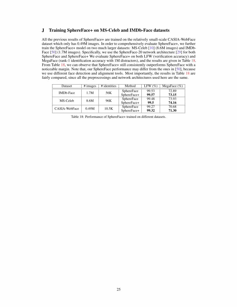
J Training SphereFace+ on MS-Celeb and IMDb-Face datasets

All the previous results of SphereFace+ are trained on the relatively small-scale CASIA-WebFacedataset which only has 0.49M images. In order to comprehensively evaluate SphereFace+, we furthertrain the SphereFace+ model on two much larger datasets: MS-Celeb [10] (8.6M images) and IMDb-Face [50] (1.7M images). Specifically, we use the SphereFace-20 network architecture [29] for bothSphereFace and SphereFace+ We evaluate SphereFace+ on both LFW (verification accuracy) andMegaFace (rank-1 identification accuracy with 1M distractors), and the results are given in Table 18.From Table 18, we can observe that SphereFace+ still consistently outperforms SphereFace with anoticeable margin. Note that, our SphereFace performance may differ from the ones in [50], becausewe use different face detection and alignment tools. Most importantly, the results in Table 18 arefairly compared, since all the preprocessings and network architectures used here are the same.

Dataset # images # identities Method LFW (%) MegaFace (%)

IMDb-Face 1.7M 56K SphereFace 99.53 72.89SphereFace+ 99.57 73.15

MS-Celeb 8.6M 96K SphereFace 99.48 73.93SphereFace+ 99.5 74.16

CASIA-WebFace 0.49M 10.5K SphereFace 99.27 70.68SphereFace+ 99.32 71.30

Table 18: Performance of SphereFace+ trained on different datasets.

25