Learning to Solve Nonlinear Least Squares

for Monocular Stereo

Ronald Clark1, Michael Bloesch1, Jan Czarnowski1, Stefan Leutenegger1, and

Andrew J. Davison1

Dyson Robotics Lab, Imperial College London, London, SW7 2AZ, UK

{ronald.clark, michael.bloesch, jan.czarnowski, s.leutenegger,

a.davison}@imperial.ac.ukhttps://www.imperial.ac.uk/dyson-robotics-lab/projects/

Abstract. Sum-of-squares objective functions are very popular in computer vi-

sion algorithms. However, these objective functions are not always easy to op-

timize. The underlying assumptions made by solvers are often not satisfied and

many problems are inherently ill-posed. In this paper, we propose a neural non-

linear least squares optimization algorithm which learns to effectively optimize

these cost functions. The proposed solver requires no hand-crafted regularizers

or priors as these are implicitly learned from the data. We apply our method to

the problem of motion stereo ie. jointly estimating the motion and scene geom-

etry from pairs of images of a monocular sequence. We show that our learned

optimizer is able to efficiently and effectively solve this challenging optimization

problem.

Keywords: Optimization · SLAM · Least Squares · Gauss-Newton · Levenberg-

Marquadt

1 Introduction

Most algorithms in computer vision use some form of optimization to obtain a solution

that best satisfies some objective function for the problem at hand. The optimization

method itself can be seen as simply an intelligent means of searching the solution space

for the answer, possibly exploiting the specific structure of the objective function to

guide the search.

One particularly interesting form of objective function is one that is composed of a

sum of many squared residual terms.

E =1

2

∑

j

r2j (x) (1)

where rj is the j-th residual term and E is the optimization objective.

In most cases the residual terms are a nonlinear function of the optimization vari-

ables and problems with this type of objective function are called nonlinear least square

(NLLS) problems (NLSPs). NLSPs can be efficiently solved using second-order meth-

ods [12].

2 Clark, et al.

However, the success in finding a good solution also depends on the characteristics

of the problem itself. The set of residual functions can be likened to a system of equa-

tions with their solution at zero, rj(x) = 0. If the number of variables in this system

is larger than the number of equations then the system is underdetermined, if they are

equal then it is well-determined and if there are more equations than variables then it

is overdetermined. Well-posed problems need to satisfy three conditions: 1) a solution

must exist 2) there must be a unique solution and 3) the solution must be continuous as

a function of its parameters [19].

Undetermined problems are ill-posed as they have infinitely many solutions and

therefore no unique solution exists. To cope with this, traditional optimizers use hand-

crafted regularizers and priors to make the ill-posed problem well-posed.

In this paper we aim to utilize strong and well-developed ideas from traditional

nonlinear least squares solvers and integrate these with the promising new learning-

based approaches. In doing so, we seek to capitalize on the ability of neural network-

based methods to learn robust data-driven priors, and a traditional optimization-based

approach to obtain refined solutions of high-precision. In particular, we propose to learn

how to compute the update based on the current residual and Jacobian (and some extra

parameters) to make the NLLS optimization algorithm more efficient and more robust

to high noise.

We apply our optimizer to the problem of estimating the pose and depths of pairs of

frames from a monocular image sequence known as monocular stereo as illustrated in

Fig. 1.

To summarise, the contributions of our paper are the following:

1. We propose an end-to-end trainable optimization method that builds upon the pow-

erful approximate Hessian-based optimization approaches to NLLS problems.

2. The implicit learning of priors and regularizers for least squares problems directly

from data.

3. The first approach to use a learned optimizer for efficiently minimizing photometric

residuals for monocular stereo reconstruction.

Compared to existing learning-based approaches, our method is designed to produce

predictions that are accurate and photometrically consistent.

The rest of the paper is structured as follows. First we outline related work on dense

reconstruction using traditional and learning-based approaches. We then visit some pre-

liminaries such as the structure of traditional Gauss-Newton optimizers for nonlinear

least square problems. We then introduce our proposed system and finally carry out an

evaluation of our method in terms of structure and motion accuracy on a number of

sequences from publicly available datasets.

2 Related Work

Optimization for SLAM In visual SLAM we are faced with the problem of estimating

both the geometry of the scene and the motion of the camera. This is most often formu-

lated as an optimization over the pixel depths and transformation parameters between

pairs of frames. The cost function comprises some form of reprojection error which

Learning to Solve Underdetermined NLSPs 3

may be formulated either in terms of geometric or photometric residuals. Geometric

residuals require the correspondence of points to be known and thus are only feasi-

ble for sparse recostructions. Photometric residuals are formulated in terms of intensity

differences and can be computed across the entire image. However, this photometric

optimization is difficult as the photometric residuals have high noise levels and vari-

ous strategies have been proposed to cope with this. In DTAM [15], for example, this

is accomplished by formulating a cost volume and integrating the residuals from mul-

tiple frames before performing the optimization. Even then, the residuals need to be

combined with a TV-L1 regularization term to ensure noise does not dominate the re-

construction. Other approaches, such as LSD-SLAM [9], operate only on high-gradient

pixels where the signal-to-noise ratio of the photometric residual is high. Even so, none

of these systems are able to estimate the geometry and motion in a single joint optimiza-

tion. Rather, they resort to an approach which swithches between independently opti-

mizing the motion parameters and then the depths in an alternating fashion. CodeSLAM

[2] overcomes this problem by using an autoencoder to compress the scene geometry

into a small optimizable code, allowing for the joint optimization of both the geometry

and motion.

Learning for Monocular Stereo There has been much interest recently in using

end-to-end learning to estimate the motion of a camera [6, 5, 22] and reconstruct scenes

from monocular images [8]. Most of these [8, 23] are based on feed-forward inference

networks. The training signal for these networks can be obtained in many ways. The

first approaches were based on a fully-supervised learning signal where labelled depth

and pose information were used. Subsequent works have shown that the networks can

be learned in a self-supervised manner using a learning signal derived, for example,

from photometric error of pixel-wise reprojection [23], from the consistency of rays

projected into a common volume [20] or even using an adversarial signal by modelling

the image formation process in a GAN framework [4]. Even so, these approaches only

utilize the photometric consistency in an offline manner, i.e. during training, and do not

attempt to optimize it online as is common in traditional dense reconstruction methods.

To this extent, some works such as [21], have demonstrated that it is beneficial to

include multiple views and a recurrent refinement procedure in the reconstruction pro-

cess. Their network, comprising three stages, is closely related to the structure which we

build on in this work. The first stage consists of a bootstrap network which produces a

Fig. 1. Overview of our system for jointly optimizing a nonlinear least squares objective

4 Clark, et al.

rough low-resolution prediction; the second stage consists of an iterative network which

iteratively refines the bootstrap prediction; and finally a refinement network which com-

putes a refined and upscaled depth map.

In this paper, we adopt the same structure but formalize the iterative network as an

optimization designed to enforce multiview photometric consistency where the boot-

strap network acts as an initialization of the optimization and the refinement acts as

an upscaling. In essence, our reconstruction is based on an optimization procedure that

is itself optimized using data. This is commonly referred to in the machine-learning

literature as a meta-learned optimizer.

Meta-learning and Learning to Optimize A popular and very promising avenue

of research which has been receiving increasing attention is that of meta-learned op-

timizers. Such approaches have shown great utility in performing few-shot learning

without overfitting [17], for optimizing GANS which are traditionally very difficult to

train [14], for optimizing general black box functions [3] and even for solving difficult

combinatorial problems [7]. Perhaps the most important advantage is to learn data-

driven regularization as demonstrated in [16] where the authors use a partially learned

optimization approach for solving ill-posed inverse problems. In [13], the authors train

through a multi-step inverse compositional Lukas Kanade algorithm for aligning 2D

images. In our method, we utilize a learned multi-step optimization model by using a

recurrent network to compute the update steps for the optimization variables. While

most approaches that attempt to learn optimization updates, such as [3], have only used

knowledge about the objective and first-order gradient information, we exploit the least-

square structure of our problem and forward the full Jacobian matrix to provide the net-

work with richer information. Our approach is – to the best of our knowledge – the first

to use second-order approximations of the objective to learn optimization updates.

3 Preliminaries

3.1 Nonlinear Least Squares Solvers

Many optimization problems have an objective that takes the form of a sum of squared

residual terms, E = 1

2

∑

j r2j (x) where rj is the j-th residual term and E is the opti-

mization objective. As such, much research has been devoted to finding efficient solvers

for problems of this form. Two of the most successful and widely used approaches are

the Gauss-Newton (GN) and Levenberg-Marquadt (LM) methods. Both of these are

second-order, iterative optimization methods. However, instead of computing the true

Hessian, they exploit the least-squares structure of the objective to compute an approx-

imate Hessian that is used in the updates. Given an initial estimate of the variables, x0,

these approaches compute updates to the optimization variable in the attempt to find a

better solution, xi, at each step i. The incremental update, ∆xi is computed by solving

a linear least squares problem which is formed by linearising the residual at the current

estimate r(xi +∆xi) ≈ ri + Ji∆xi [12], with the abbreviations:

ri = r(xi), Ji =dr

dx

∣

∣

∣

∣

x=xi

. (2)

Learning to Solve Underdetermined NLSPs 5

Using the linearized residual, the optimal update can be found as the solution to the

quadratic problem [12]

∆xi = argmin∆xi

1

2||ri + Ji∆xi||

2. (3)

The well known Normal equations to this can be computed analytically by differenti-

ating the problem and equating to zero. The update step used in GN is then given by

solving:

JTi Ji∆xi = −JT

i ri (4)

By comparing this to Newton’s method which requires the computation of the true

Hessian H(xi) for finding updates [10], we see that the GN method effectively approx-

imates H(xi) using JTi Ji, which is usually more efficient to compute. LM extends GN

by adding a damping factor λ to the update ∆xi = −(JTi Ji + λ diag(JT

i Ji))−1JT

i rito better condition the updates and make the optimization more robust [10].

In our proposed approach, we build on the GN method by not restricting the updates

to be a static function of Ji. Compared to LM which adaptively sets a single parameter,

λ, we compute the entire update step by using a neural network which has as its input

the full Jacobian Ji. The details of this are described in Section 4.2.

3.2 Warping and Photometric Cost Function

The warping function we use for the least squares cost function is similar to the loss used

in the usupervised training in [23]. The warping is based on a spatial transformer which

first transforms the coordinates of points in the target view to points in the source view

and then samples the source view. The 4x4 transformation matrix, Tt→s is obtained by

applying an exponential map to the output of the network, i.e. Tt→s = exp (p×) where

p (bold face) is the relative pose represented as a six-vector and ps (non-bold face) is

the pixel location in the source image and pt (non-bold face) is a pixel location in the

target image (consistent with the notation in the paper)

ps ∼ KTt→sDt(pt)K−1pt (5)

Using these warped coordinates, a synthesized image Is(p) is obtained through bi-

linear sampling of the the source view at the locations ps computed in Eqn. 5. The least

squares loss function from which we derive J is then,

L =∑

p

||It(p)− Is(p)||2 , (6)

where It and Is are the source and target intensity images and the residual cor-

responding to each pixel is rp = It(p) − Is(p). The elements of the Jcaobian of

the warping function, J, can be easily computed using autodiff (in Tensorflow simply

tf.gradients(res[i],x)) for each residual. However, to speed up our imple-

mentation we anylytically compute the elements of the Jacobian in our computation

graph.

6 Clark, et al.

4 Model

The model is built around the optimization of the photometric consistency of the depth

and motion predictions for a short sequence of input images. Each sequence of images

has a single “target” keyframe (which we choose as the first frame) for which we opti-

mize the depth values. In all cases, we operate on inverse depths, z = 1

dfor better han-

dling of large depths values. Our model additionally seeks to optimize for the relative

transformations between each source frame s in the sequence and the target keyframe

t, pt→s. The full model consists of three stages. All iterative optimization procedures

require an initial starting point and thus the initialization stage serves the purpose of

predicting a good initial estimate. The optimization stage consists of a learned opti-

mizer which benefits from explicitly computed residuals and Jacobians. To make the

optimization computationally tractable, the optimization network operates on a down-

sampled version of the input and exploits the sparsity of the problem. The final stage of

the network upsamples the prediction to the original resolution. The networks (includ-

ing those of the optimizer) are trained using a supervised loss. We now describe each

of the three network components in detail.

Algorithm 1 Neuro-Adaptive Nonlinear Least Squares

Require: Residual function r(x), image sequence I1, I2, . . .

x0 ← fθ0(I1, I2, . . .)for i = 0, 1, . . . N − 1 do

∆xi,hi+1 ← fθ (Φ(Ji, ri),hi)if ||∆xi|| < ǫ then

return xi

end if

xi+1 ← xi +∆xi

end for

4.1 Initialization Network

The purpose of the initialization network is to predict a suitable starting point for the

optimization stage. We provide the initialization network with both RGB images and

thereby allow it to leverage stereopsis. The architecture of this stage is a simple con-

volutional network. For this stage we use 3 convolutions with stride 2, one convolution

with stride 1 and one upsamplings + convolutional layers. This results in the output of

the network being downscaled by a factor of 4 for feeding into the optimization stage.

The network also produces an initial pose using a fully connected layer branched from

the central layers of the network. Thus the output of the initialization stage consists of

an initial depth image and pose.

4.2 Neuro-Adaptive Nonlinear Least Squares

The learnt optimization procedure is outlined in Algorithm 1. The optimization net-

work attempts to optimize the photometric objective E(x) where x = (z,p) are the

Learning to Solve Underdetermined NLSPs 7

optimization variables (inverse depths z and pose p). The objective E(x) is a nonlinear

least squares expression defined in terms of the photometric residual vector r(x)

E(x) =1

2||r(x)||2. (7)

The updates of the parameters to be optimized, x, follow a standard iterative opti-

mization scheme, i.e.

xi+1 = xi +∆xi. (8)

In our case, the updates ∆xi are predicted using a Long Short Term Memory Recurrent

Neural Network (LSTM-RNN) [11]. In order to compute the Jacobian we use auto-

matic differentiation available in the Tensorflow library [1]. Using the automatic differ-

entiation operation, we add operations to the Tensorflow computation graph [1] which

compute the Jacobian of our residual vector with respect to the dense depth and motion.

As the structure of the Jacobian often exhibits problem specific properties, we apply a

transformation to the Jacobian, Φ(Ji, ri) before feeding this Jacobian into our network.

The operation Φ may involve element-wise matrix operations such as gather or other

operations which simplify the Jacobian input. The operations we use for the problems

addressed in this paper are detailed in Section 4.3.

To allow for the computation of parameter updates which are not restricted to those

derived from the approximate Hessian, we turn to the powerful function approximation

ability of the LSTM-RNN [11] to learn the final parameter update operation from data.

As the number of coordinates are likely to be very large for most optimization problems,

[3] propose to use one LSTM-RNN for each coordinate. For our problem, we have

Jacobians with high spatial correlations and thus we replace the coordinate-wise LSTM

with a convolutional LSTM. The per-iteration updates, ∆xi are predicted by a network

which in this case is an LSTM-RNN,[

∆xi

hi+1

]

= LSTMcell (Φ(Ji, ri), hi,xi; θ) , (9)

where θ are the parameters of the networks and LSTMcell is a standard LSTM cell

update function with hidden layer hi.

4.3 The Jacobian input structure

Each type of least squares cost function gives rise to a special Jacobian structure. The

input function, Φ(J, r), to our network serves two purposes; one functional and the

other structural. Firstly, Φ serves to compute the approximate Hessian as is done with

the classical Gauss-Newton optimization method:

Φ(J, r) = [JTJ, r]. (10)

The structure of Φ(J, r) is shown in Figure 2. We note that we choose not to compute

the full (JTJ)−1J as this adds additional computational complexity to the operation

which is repeated many times during training. We also compress the sparse JTJ into a

compact form as illustrated in Figure 2. The output of this restructuring yields the same

image shape as the image. The compressed structure allows efficient processing of the

matrix.

8 Clark, et al.

Fig. 2. The block-sparsity structure of J and JTJ for the depth and egomotion estimation prob-

lem.

4.4 Upscaling Network

As the optimization network operates on low-resolution predictions, an upscaling net-

work is used to produce outputs of the desired size. The upscaling network consists of a

series of bilinear upsampling layers concatenated with convolutions and acts as a super-

resolution network. The input to the upscaling network consists of the low-resolution

depth prediction and the RGB image.

5 Loss Function

In this section we describe the loss function which we use to train the network weights

of all three stages of our model.

The current state-of-the-art depth and motion prediction networks still rely on la-

belled images to provide a strong learning signal. We include a loss term based on

labelled ground truth inverse depth images z,

Ldepth(x) =1

wh‖z− z‖1 (11)

with image width w and height h, and where z is the predicted inverse depth image.

We also use a loss term based on the relative pose between the source (s) and target

(t) frame, p = (tt→s, αt→s) with translation tt→s and rotation vector αt→s from

ground-truth data,

Lpose(x) =∑

s

‖αt→s − αt→s‖1 + ‖tt→s − tt→s‖1 (12)

Note that this loss function need not be a sum of squares and can be computed using any

other form using eg. L1 etc. The final loss function consists of a weighted combination

of the individual loss terms:

Ltot(θ) =∑

i

wposeLpose(xi(θ)) + wdepthLdepth(xi(θ)). (13)

Learning to Solve Underdetermined NLSPs 9

Note that our objective here includes the ground-truth inverse depth which we do not

have access to when computing the residuals r (and then the Jacobian J) in the recurrent

optimization network in Section 4.2.

The optimization network is never directly privy to the ground truth depth and poses,

it only benefits from these by what is learned in the network parameters during training.

In this manner, we have a system which is trained offline to best minimize our objec-

tive online. During the offline training phase, our system learns robust priors for the

optimization by using the large amounts of labelled data. During the online phase our

system optimizes for photometric consistency only but is able to utilize the knowledge

it has learned during the offline training to better condition the optimization process.

6 Training

During the training, we unroll our iterative optimization network for a set number of

steps and backpropogate the loss through the network weights, θ. In order to find the

parameters of the optimizer network, the meta-loss, Ltot(θ), is minimized using the

ADAM optimizer where the total meta-loss is computed as the loss summed over the N

iterations of the learned optimization (see Eq. 13). For each step i in the optimization

process we update the state xi of the optimization network according to Eqn. 8.

As our loss depends on variables which are updated recurrently over a number of

timesteps, we use backpropogation through time to train the network. Backpropogation

through time unrolls each step and updates the parameters by computing the gradients

through the unrolled network. In our experiments we unroll our optimization for 15

steps.

We find that training the whole network at once is difficult and thus train the initial-

ization network first before adding the optimization stage.

7 Evaluation

In this section we evaluate the proposed method on both synthetic and real datasets.

We aim to determine the efficiency of our approach i.e. how quickly it converges to an

optimum and how it compares to a network which does not explicitly incorporate the

problem structure in its iterations.

7.1 Synthetic data experiments

In this section we evaluate the performance of our proposed method on a number of

least squares curve fitting problems. We experiment on curves parameterized by two

variables, x = (a, b). We chose a set of four functions to use for our experiment as

follows

y = x exp(at) + x exp(bt) + ǫ, (14)

y = sin(at+ b) + ǫ, (15)

y = sinc(at+ b) + ǫ, (16)

10 Clark, et al.

y = N (t|µ = a, σ = b) (fitting a Gaussian) (17)

For these experiments we generate the data by randomly sampling one of four para-

metric functions (Eqn. 14 to Eqn. 17) as well as the two parameters a and b. For the

training data we add noise ǫ ∼ N (0, 0.1) to the true function values. In Figure 3 we

show the results on a test set of sampled functions. Figure 3 a) shows the fitted func-

tion after 5 iterations (of a total of 15 iterations) for our method and standard LM. The

learned approach clearly outperforms LM in terms of speed of convergence. In Figure

3 b) we see the learned errors vs LM for all steps in the optimization, where again, the

learned method clearly outperforms LM.

0 5 10 15 20 25 30

0.0

0.5

1.0

1.5

2.0Original data

NeuNo

LM

Iteration

Obje

cti

ve

1 3 5 7 9

Iteration no.

0.0

0.1

0.2

0.3

0.4

Obje

cti

ve

Proposed

LM

0.0 0.1 0.2 0.3 0.4 0.5

Levenberg-Marquadt error

0.0

0.1

0.2

0.3

0.4

0.5

NeuN

o E

rror

Fig. 3. Comparison between our method and standard least squares for fitting parametric func-

tions to noisy data with a least-squares objective. In a) the fitted functions limited to 5 iterations

is shown, in b) the error as a function of iteration no. is shown for 10 test functions and in c) the

LM error is plotted against the error of the proposed method for all iterations.

7.2 Real-world test: depth and pose estimation

In this section we test the ability of our proposed method on estimating the depth and

egomotion of a moving camera. To provide a fair evaluation of the proposed approach,

we use the same evaluation procedure as in [21] and report the same baselines, where

oracle uses MVS with known poses, SIFT uses sparse-feature for correspondences, FF

uses optical flow, Matlab uses the KLT tracker in Matlab as the basis of a bundle-

adjusted reconstruction.

7.3 Metrics

We evaluate the performance of our approach on the depth as well as the motion predic-

tion performance. For depth prediction we use the absolute, scale-invariant and relative

performance metrics.

7.4 Datasets

The datasets which we use to evaluate the network consist of both indoor and outdoor

scenes. For all the datasets, the camera undergoes free 6-DoF motion. To train our

network we use images from all the datasets partitioned into testing and training sets.

Learning to Solve Underdetermined NLSPs 11

Fig. 4. Qualitative results on two challenging indoor scenes using only two frames. The figure

shows the last 5 iterations of 15 of the optimization network. Even with this wide baseline, and

only two frames, our method is able to optimize the photometric error reliably.

MVS The multiview stereo dataset consists of a collection of scenes obtained using

struction from motion software followed by dense multi-view stereo reconstruction.

We use the same training/test split as in [21]. The training set of images used included

“Citywall”, “Achteckturm” and “Breisach” scenes with “Person-Hall”, “Graham-Hall”,

and “South-Building” for testing.

TUM The TUM RGB-D dataset consists of Kinect-captured RGB-D image sequences

with ground truth poses obtained from a Vicon system. It comprises a total of 19 se-

quences with 45356 images. We use the same test / train split as in [21] with 80 held-out

images for test.

Sun3D The SUN3D dataset consists of scenes reconstructed using RGB-D structure-

from-motion. The dataset has a variety of indoor scenes, with absolute scale and con-

sists of 10,000 individual images. The poses are less accurate than the TUM dataset as

they were obtained using an RGB-D reconstruction.

A qualitative evaluation of our method compared to standard multiview stereo and

DeMoN [21] is shown in Figure 5. Our method produces depth maps with sharper struc-

tures compared to DeMoN, even with a lower output resolution. Compared to COLMAP

[18] our reconstruction is more dense and does not include as many outlier pixels. Nu-

merical results on the testing data-sets are shown in Table 1. As is evident from the

12 Clark, et al.

Img1 Img2 Ours DeMoN GTImg1 Img2 Ours DeMoN GT

Img1 Img2 Ours DeMoN GTImg1 Img2 Ours DeMoN GT

Fig. 5. Qualitative results on the NYU dataset. Compared to DeMoN our network has fewer

”hallucinations” of structures which do not exist in the scene.

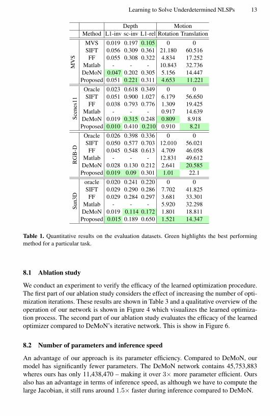
Table, our learned optimization approach outperforms most of the traditional baseline

approaches, and performs better or on par with DeMoN on most cases. This may be

due to our architectural choice as we do not include any alternating flow and depth

predictions.

8 Discussion

In the context of optimisation, our network-based updates accomplish something which

a classical optimisation approach cannot in that it is able to reliably optimise a large

under-determined system with implicitly learned priors.

Table 2. Summary of the performance of our

Neuro-Adaptive optimisation compared to stan-

dard LM. Table indicates the best performing

method for criteria.Problem Size

Small Medium Large

Accuracy Ours Ours Ours

Memory Tie Ours Ours

Speed Tie Ours Ours

For a large under-determined problem

like in the depth and motion case, stan-

dard Levenberg-Marquadt (LM) fails to

improve the objective and the required

sparse matrix inversion for a JTJ with

≈ 91K non-zero elements (128 × 96

size image) takes 532ms, compared to

our network forward pass which takes

25ms. For small, overdetermined prob-

lems LM does work and for this reason,

in Section 7.1, we have compared our approach to LM on a small curve fitting prob-

lem and found that our approach significantly outperforms it in terms of accuracy and

convergence rate. For the small problem, the matrix inversion in the standard approach

(LM) is very quick but we are also able to use a smaller network so our time per-iteration

is tie with LM. This is summarised in Table 8.

Learning to Solve Underdetermined NLSPs 13

Depth Motion

Method L1-inv sc-inv L1-rel Rotation Translation

MV

S

MVS 0.019 0.197 0.105 0 0

SIFT 0.056 0.309 0.361 21.180 60.516

FF 0.055 0.308 0.322 4.834 17.252

Matlab - - - 10.843 32.736

DeMoN 0.047 0.202 0.305 5.156 14.447

Proposed 0.051 0.221 0.311 4.653 11.221S

cen

es1

1

Oracle 0.023 0.618 0.349 0 0

SIFT 0.051 0.900 1.027 6.179 56.650

FF 0.038 0.793 0.776 1.309 19.425

Matlab - - - 0.917 14.639

DeMoN 0.019 0.315 0.248 0.809 8.918

Proposed 0.010 0.410 0.210 0.910 8.21

RG

B-D

Oracle 0.026 0.398 0.336 0 0

SIFT 0.050 0.577 0.703 12.010 56.021

FF 0.045 0.548 0.613 4.709 46.058

Matlab - - - 12.831 49.612

DeMoN 0.028 0.130 0.212 2.641 20.585

Proposed 0.019 0.09 0.301 1.01 22.1

Su

n3

D

oracle 0.020 0.241 0.220 0 0

SIFT 0.029 0.290 0.286 7.702 41.825

FF 0.029 0.284 0.297 3.681 33.301

Matlab - - - 5.920 32.298

DeMoN 0.019 0.114 0.172 1.801 18.811

Proposed 0.015 0.189 0.650 1.521 14.347

Table 1. Quantitative results on the evaluation datasets. Green highlights the best performing

method for a particular task.

8.1 Ablation study

We conduct an experiment to verify the efficacy of the learned optimization procedure.

The first part of our ablation study considers the effect of increasing the number of opti-

mization iterations. These results are shown in Table 3 and a qualitative overview of the

operation of our network is shown in Figure 4 which visualizes the learned optimiza-

tion process. The second part of our ablation study evaluates the efficacy of the learned

optimizer compared to DeMoN’s iterative network. This is show in Figure 6.

8.2 Number of parameters and inference speed

An advantage of our approach is its parameter efficiency. Compared to DeMoN, our

model has significantly fewer parameters. The DeMoN network contains 45,753,883

wheres ours has only 11,438,470 – making it over 3× more parameter efficient. Ours

also has an advantage in terms of inference speed, as although we have to compute the

large Jacobian, it still runs around 1.5× faster during inference compared to DeMoN.

14 Clark, et al.

Depth Motion

Method L1-inv sc-inv L1-rel Rotation Translation

RG

B-D

Initialization 0.260 0.360 0.315 2.290 27.40

Opt (5 steps) 0.220 0.15 0.308 2.11 25.63

Opt (10 steps) 0.21 0.12 0.310 1.23 24.91

Opt (15 steps) 0.019 0.09 0.301 1.01 22.14

Table 3. Results of the ablation study to evaluate the performance of the optimization iterations.

1 2 3 4 5 6

Iteration No.

0

0.005

0.01

0.015

0.02

0.025

0.03

0.035

0.04

0.045

L1-i

nv

Err

or

on

SU

N3D

DeMon .

Ours

(Std RNN)

Fig. 6. Comparison between our learned optimizer and the (larger) RNN refinement network from

DeMon.

9 Conclusion

In this paper we have presented an approach for robustly solving nonlinear least squares

optimization problems by integrating deep neural models with traditional knowledge of

the optimization structure. Our method is based on a novel neuro-adaptive nonlinear

least squares optimizer which is trained to robustly optimize the residuals. Although

it is generally applicable to any least squares problem, we have demonstrated the pro-

posed method on the real-world problem of computing depth and egomotion for frames

of a monocular video sequence. Our method can cope with images captured from a

wide baseline. In future work we plan to investigate means of increasing the number

of residuals that are optimized and thereby achieve an even more detailed prediction.

We also plan to further study the interplay between the recurrent neural network and

optimization structure and want to investigate the use of predicted confidence estimates

in the learned optimization.

References

1. Abadi, M., Agarwal, A., Barham, P., Brevdo, E., Chen, Z., Citro, C., Corrado, G.S., Davis,

A., Dean, J., Devin, M., et al.: Tensorflow: Large-scale machine learning on heterogeneous

distributed systems. arXiv preprint arXiv:1603.04467 (2016)

Learning to Solve Underdetermined NLSPs 15

2. Bloesch, M., Czarnowski, J., Clark, R., Leutenegger, S., Davison, A.J.: CodeSLAM — learn-

ing a compact, optimisable representation for dense visual SLAM. In: Proceedings of the

IEEE Conference on Computer Vision and Pattern Recognition (CVPR) (2018)

3. Chen, Y., Hoffman, M.W., Colmenarejo, S.G., Denil, M., Lillicrap, T.P., Botvinick, M.,

de Freitas, N.: Learning to learn without gradient descent by gradient descent. In: Proceed-

ings of the 34th International Conference on Machine Learning. vol. 70, pp. 748–756. PMLR

(06–11 Aug 2017)

4. Choy, C.B., Xu, D., Gwak, J., Chen, K., Savarese, S.: 3d-r2n2: A unified approach for single

and multi-view 3d object reconstruction. In: Proceedings of the European Conference on

Computer Vision (ECCV) (2016)

5. Clark, R., Wang, S., Wen, H., Markham, A., Trigoni, N.: VidLoc: A deep spatio-temporal

model for 6-dof video-clip relocalization. In: Proceedings of the IEEE Conference on Com-

puter Vision and Pattern Recognition (CVPR) (2017)

6. Clark, R., Wang, S., Wen, H., Markham, A., Trigoni, N.: VINet: Visual-inertial odometry

as a sequence-to-sequence learning problem. In: Proceedings of the National Conference on

Artificial Intelligence (AAAI) (2017)

7. Dai, H., Khalil, E.B., Zhang, Y., Dilkina, B., Song, L.: Learning combinatorial optimization

algorithms over graphs. arXiv preprint arXiv:1704.01665 (2017)

8. Eigen, D., Fergus, R.: Predicting Depth, Surface Normals and Semantic Labels with a Com-

mon Multi-Scale Convolutional Architecture. In: Proceedings of the International Confer-

ence on Computer Vision (ICCV) (2015)

9. Engel, J., Schoeps, T., Cremers, D.: LSD-SLAM: Large-scale direct monocular SLAM. In:

Proceedings of the European Conference on Computer Vision (ECCV) (2014)

10. Fletcher, R.: Practical methods of optimization. John Wiley & Sons (2013)

11. Hochreiter, S., Younger, A.S., Conwell, P.R.: Learning to Learn Using Gradient Descent, pp.

87–94 (2001)

12. Kelley, C.T.: Iterative methods for optimization, vol. 18. Siam (1999)

13. Lin, C.H., Lucey, S.: Inverse compositional spatial transformer networks. arXiv preprint

arXiv:1612.03897 (2016)

14. Metz, L., Poole, B., Pfau, D., Sohl-Dickstein, J.: Unrolled generative adversarial networks.

arXiv preprint arXiv:1611.02163 (2016)

15. Newcombe, R.A., Izadi, S., Hilliges, O., Molyneaux, D., Kim, D., Davison, A.J., Kohli, P.,

Shotton, J., Hodges, S., Fitzgibbon, A.: KinectFusion: Real-Time Dense Surface Mapping

and Tracking. In: Proceedings of the International Symposium on Mixed and Augmented

Reality (ISMAR) (2011)

16. Oktem, O., Adler, J.: Solving ill-posed inverse problems using iterative deep neural networks.

Inverse Problems (2017)

17. Ravi, S., Larochelle, H.: Optimization as a model for few-shot learning. International Con-

ference on Learning Representations (ICLR) (2016)

18. Schonberger, J.L., Zheng, E., Pollefeys, M., Frahm, J.M.: Pixelwise view selection for un-

structured multi-view stereo. In: European Conference on Computer Vision (ECCV) (2016)

19. Tikhonov, A., Arsenin, V.: Solutions of ill-posed problems. Winston, Washington,DC (1977)

20. Tulsiani, S., Zhou, T., Efros, A.A., Malik, J.: Multi-view supervision for single-view re-

construction via differentiable ray consistency. In: Proceedings of the IEEE Conference on

Computer Vision and Pattern Recognition (CVPR) (2017)

21. Ummenhofer, B., Zhou, H., Uhrig, J., Mayer, N., Ilg, E., Dosovitskiy, A., Brox, T.: Demon:

Depth and motion network for learning monocular stereo. In: Proceedings of the IEEE Con-

ference on Computer Vision and Pattern Recognition (CVPR)

22. Wang, S., Clark, R., Wen, H., Trigoni, N.: DeepVO: Towards end to end visual odometry

with deep recurrent convolutional neural networks. In: Proceedings of the IEEE International

Conference on Robotics and Automation (ICRA) (2017)

16 Clark, et al.

23. Zhou, T., Brown, M., Snavely, N., Lowe, D.G.: Unsupervised learning of depth and ego-

motion from video. In: Proceedings of the IEEE Conference on Computer Vision and Pattern

Recognition (CVPR) (2017)