Learning to Search Better than Your TeacherLearning to Search Better than Your Teacher)=0.2y y y x Î X e Î Y, l(y e)=0.0 e Î Y, l(y e e Î Y, l(y e)=0.8 Figure 2. An example search

Learning to Search Better than Your Teacher

Kai-Wei Chang [email protected]

University of Illinois at Urbana Champaign, IL

Akshay Krishnamurthy [email protected]

Carnegie Mellon University, Pittsburgh, PA

Alekh Agarwal [email protected]

Microsoft Research, New York, NY

Hal Daume III [email protected]

University of Maryland, College Park, MD, USA

John Langford [email protected]

Microsoft Research, New York, NY

AbstractMethods for learning to search for structured prediction typically imitate a reference policy, with existing theoret-ical guarantees demonstrating low regret compared to that reference. This is unsatisfactory in many applicationswhere the reference policy is suboptimal and the goal of learning is to improve upon it. Can learning to searchwork even when the reference is poor?

We provide a new learning to search algorithm, LOLS, which does well relative to the reference policy, butadditionally guarantees low regret compared to deviations from the learned policy: a local-optimality guarantee.Consequently, LOLS can improve upon the reference policy, unlike previous algorithms. This enables us todevelop structured contextual bandits, a partial information structured prediction setting with many potentialapplications.

1. IntroductionIn structured prediction problems, a learner makes joint predictions over a set of interdependent output variables and ob-serves a joint loss. For example, in a parsing task, the output is a parse tree over a sentence. Achieving optimal performancecommonly requires the prediction of each output variable to depend on neighboring variables. One approach to structuredprediction is learning to search (L2S) (Collins & Roark, 2004; Daume III & Marcu, 2005; Daume III et al., 2009; Rosset al., 2011; Doppa et al., 2014; Ross & Bagnell, 2014), which solves the problem by:

1. converting structured prediction into a search problem with specified search space and actions;2. defining structured features over each state to capture the interdependency between output variables;3. constructing a reference policy based on training data;4. learning a policy that imitates the reference policy.

Empirically, L2S approaches have been shown to be competitive with other structured prediction approaches both in ac-curacy and running time (see e.g. Daume III et al. (2014)). Theoretically, existing L2S algorithms guarantee that if the

arX

iv:1

502.

0220

6v2

[cs

.LG

] 2

0 M

ay 2

015


[ ]

. . .

[N ]

. . .

[N V ]

. . .

[N V V],loss=1

[N V N],loss=0[N N ][V ]

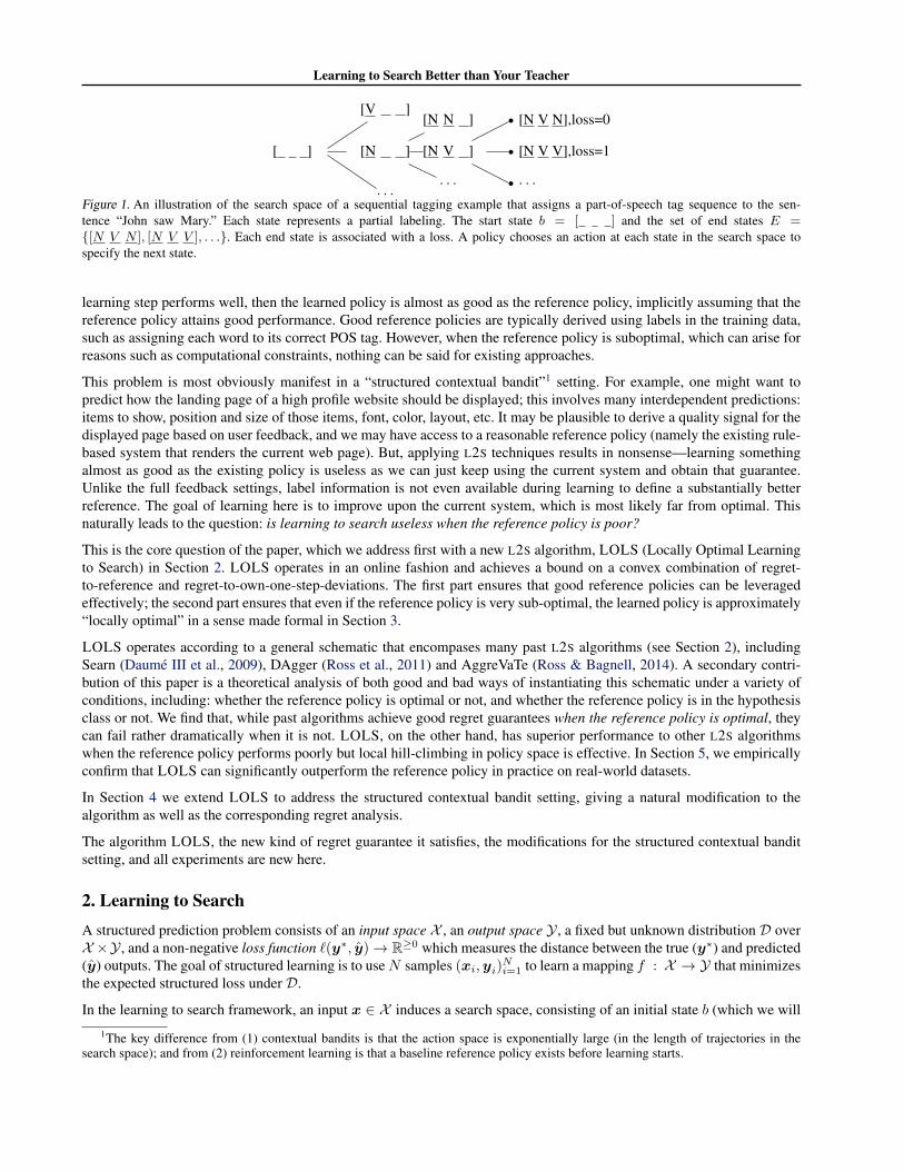
Figure 1. An illustration of the search space of a sequential tagging example that assigns a part-of-speech tag sequence to the sen-tence “John saw Mary.” Each state represents a partial labeling. The start state b = [ ] and the set of end states E =[N V N ], [N V V ], . . .. Each end state is associated with a loss. A policy chooses an action at each state in the search space tospecify the next state.

learning step performs well, then the learned policy is almost as good as the reference policy, implicitly assuming that thereference policy attains good performance. Good reference policies are typically derived using labels in the training data,such as assigning each word to its correct POS tag. However, when the reference policy is suboptimal, which can arise forreasons such as computational constraints, nothing can be said for existing approaches.

This problem is most obviously manifest in a “structured contextual bandit”1 setting. For example, one might want topredict how the landing page of a high profile website should be displayed; this involves many interdependent predictions:items to show, position and size of those items, font, color, layout, etc. It may be plausible to derive a quality signal for thedisplayed page based on user feedback, and we may have access to a reasonable reference policy (namely the existing rule-based system that renders the current web page). But, applying L2S techniques results in nonsense—learning somethingalmost as good as the existing policy is useless as we can just keep using the current system and obtain that guarantee.Unlike the full feedback settings, label information is not even available during learning to define a substantially betterreference. The goal of learning here is to improve upon the current system, which is most likely far from optimal. Thisnaturally leads to the question: is learning to search useless when the reference policy is poor?

This is the core question of the paper, which we address first with a new L2S algorithm, LOLS (Locally Optimal Learningto Search) in Section 2. LOLS operates in an online fashion and achieves a bound on a convex combination of regret-to-reference and regret-to-own-one-step-deviations. The first part ensures that good reference policies can be leveragedeffectively; the second part ensures that even if the reference policy is very sub-optimal, the learned policy is approximately“locally optimal” in a sense made formal in Section 3.

LOLS operates according to a general schematic that encompases many past L2S algorithms (see Section 2), includingSearn (Daume III et al., 2009), DAgger (Ross et al., 2011) and AggreVaTe (Ross & Bagnell, 2014). A secondary contri-bution of this paper is a theoretical analysis of both good and bad ways of instantiating this schematic under a variety ofconditions, including: whether the reference policy is optimal or not, and whether the reference policy is in the hypothesisclass or not. We find that, while past algorithms achieve good regret guarantees when the reference policy is optimal, theycan fail rather dramatically when it is not. LOLS, on the other hand, has superior performance to other L2S algorithmswhen the reference policy performs poorly but local hill-climbing in policy space is effective. In Section 5, we empiricallyconfirm that LOLS can significantly outperform the reference policy in practice on real-world datasets.

In Section 4 we extend LOLS to address the structured contextual bandit setting, giving a natural modification to thealgorithm as well as the corresponding regret analysis.

The algorithm LOLS, the new kind of regret guarantee it satisfies, the modifications for the structured contextual banditsetting, and all experiments are new here.

2. Learning to SearchA structured prediction problem consists of an input space X , an output space Y , a fixed but unknown distribution D overX ×Y , and a non-negative loss function `(y∗, y)→ R≥0 which measures the distance between the true (y∗) and predicted(y) outputs. The goal of structured learning is to useN samples (xi,yi)

Ni=1 to learn a mapping f : X → Y that minimizes

the expected structured loss under D.

In the learning to search framework, an input x ∈ X induces a search space, consisting of an initial state b (which we will

1The key difference from (1) contextual bandits is that the action space is exponentially large (in the length of trajectories in thesearch space); and from (2) reinforcement learning is that a baseline reference policy exists before learning starts.


s r e

e

e

rollin

rollout one-step

deviations

x Xy

eY, l(y

e)=0.0

yeY, l(y

e)=0.2

yeY, l(y

e)=0.8

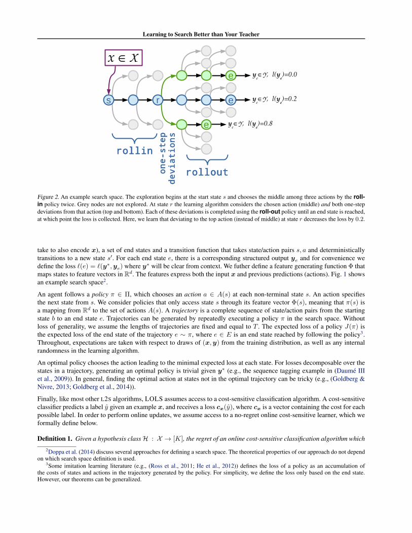
Figure 2. An example search space. The exploration begins at the start state s and chooses the middle among three actions by the roll-in policy twice. Grey nodes are not explored. At state r the learning algorithm considers the chosen action (middle) and both one-stepdeviations from that action (top and bottom). Each of these deviations is completed using the roll-out policy until an end state is reached,at which point the loss is collected. Here, we learn that deviating to the top action (instead of middle) at state r decreases the loss by 0.2.

take to also encode x), a set of end states and a transition function that takes state/action pairs s, a and deterministicallytransitions to a new state s′. For each end state e, there is a corresponding structured output ye and for convenience wedefine the loss `(e) = `(y∗,ye) where y∗ will be clear from context. We futher define a feature generating function Φ thatmaps states to feature vectors in Rd. The features express both the input x and previous predictions (actions). Fig. 1 showsan example search space2.

An agent follows a policy π ∈ Π, which chooses an action a ∈ A(s) at each non-terminal state s. An action specifiesthe next state from s. We consider policies that only access state s through its feature vector Φ(s), meaning that π(s) isa mapping from Rd to the set of actions A(s). A trajectory is a complete sequence of state/action pairs from the startingstate b to an end state e. Trajectories can be generated by repeatedly executing a policy π in the search space. Withoutloss of generality, we assume the lengths of trajectories are fixed and equal to T . The expected loss of a policy J(π) isthe expected loss of the end state of the trajectory e ∼ π, where e ∈ E is an end state reached by following the policy3.Throughout, expectations are taken with respect to draws of (x,y) from the training distribution, as well as any internalrandomness in the learning algorithm.

An optimal policy chooses the action leading to the minimal expected loss at each state. For losses decomposable over thestates in a trajectory, generating an optimal policy is trivial given y∗ (e.g., the sequence tagging example in (Daume IIIet al., 2009)). In general, finding the optimal action at states not in the optimal trajectory can be tricky (e.g., (Goldberg &Nivre, 2013; Goldberg et al., 2014)).

Finally, like most other L2S algorithms, LOLS assumes access to a cost-sensitive classification algorithm. A cost-sensitiveclassifier predicts a label y given an example x, and receives a loss cx(y), where cx is a vector containing the cost for eachpossible label. In order to perform online updates, we assume access to a no-regret online cost-sensitive learner, which weformally define below.

Definition 1. Given a hypothesis classH : X → [K], the regret of an online cost-sensitive classification algorithm which

2Doppa et al. (2014) discuss several approaches for defining a search space. The theoretical properties of our approach do not dependon which search space definition is used.

3Some imitation learning literature (e.g., (Ross et al., 2011; He et al., 2012)) defines the loss of a policy as an accumulation ofthe costs of states and actions in the trajectory generated by the policy. For simplicity, we define the loss only based on the end state.However, our theorems can be generalized.


Algorithm 1 Locally Optimal Learning to Search (LOLS)Require: Dataset xi,yiNi=1 drawn from D and β ≥ 0: a mixture parameter for roll-out.

1: Initialize a policy π0.2: for all i ∈ 1, 2, . . . , N (loop over each instance) do3: Generate a reference policy πref based on yi.4: Initialize Γ = ∅.5: for all t ∈ 0, 1, 2, . . . , T − 1 do6: Roll-in by executing πin

i = πi for t rounds and reach st.7: for all a ∈ A(st) do8: Let πout

i =πref with probability β, otherwise πi.9: Evaluate cost ci,t(a) by rolling-out with πout

i for T − t− 1 steps.10: end for11: Generate a feature vector Φ(xi, st).12: Set Γ = Γ ∪ 〈ci,t,Φ(xi, st)〉.13: end for14: πi+1 ← Train(πi,Γ) (Update).15: end for16: Return the average policy across π0, π1, . . . πN .

produces hypotheses h1, . . . , hM on cost-sensitive example sequence (x1, c1), . . . , (xM , cM ) is

RegretCSM =

M∑m=1

cm(hm(xm))−minh∈H

M∑m=1

cm(h(xm)). (1)

An algorithm is no-regret if RegretCSM = o(M).

Such no-regret guarantees can be obtained, for instance, by applying the SECOC technique (Langford & Beygelzimer,2005) on top of any importance weighted binary classification algorithm that operates in an online fashion, examples beingthe perceptron algorithm or online ridge regression.

LOLS (see Algorithm 1) learns a policy π ∈ Π to approximately minimize J(π),4 assuming access to a reference policyπref (which may or may not be optimal). The algorithm proceeds in an online fashion generating a sequence of learnedpolicies π0, π1, π2, . . .. At round i, a structured sample (xi,yi) is observed, and the configuration of a search space isgenerated along with the reference policy πref. Based on (xi,yi), LOLS constructs T cost-sensitive multiclass examplesusing a roll-in policy πin

i and a roll-out policy πouti . The roll-in policy is used to generate an initial trajectory and the roll-out

policy is used to derive the expected loss. More specifically, for each decision point t ∈ [0, T ), LOLS executes πini for t

rounds reaching a state st ∼ πini . Then, a cost-sensitive multiclass example is generated using the features Φ(st). Classes

in the multiclass example correspond to available actions in state st. The cost c(a) assigned to action a is the difference inloss between taking action a and the best action.

c(a) = `(e(a))−mina′

`(e(a′)), (2)

where e(a) is the end state reached with rollout by πouti after taking action a in state st. LOLS collects the T examples from

the different roll-out points and feeds the set of examples Γ into an online cost-sensitive multiclass learner, thereby updatingthe learned policy from πi to πi+1. By default, we use the learned policy πi for roll-in and a mixture policy for roll-out.For each roll-out, the mixture policy either executes πref to an end-state with probability β or πi with probability 1 − β.LOLS converts into a batch algorithm with a standard online-to-batch conversion where the final model π is generated byaveraging πi across all rounds (i.e., picking one of π1, . . . πN uniformly at random).

4 We can parameterize the policy π using a weight vector w ∈ Rd such that a cost-sensitive classifier can be used to choose an actionbased on the features at each state. We do not consider using different weight vectors at different states.


roll-out→

↓ roll-inReference Mixture Learned

Reference Inconsistent

Learned Not locally opt. Good RL

Table 1. Effect of different roll-in and roll-out policies. The strategies marked with “Inconsistent” might generate a learned policy witha large structured regret, and the strategies marked with “Not locally opt.” could be much worse than its one step deviation. The strategymarked with “RL” reduces the structure learning problem to a reinforcement learning problem, which is much harder. The strategymarked with “Good” is favored.

s1

s3

e4, 0fe3, 100eb

s2

e2, 10de1, 0c

a

(a) πini =πout

i =πref

s1

s3

e4, 0fe3, 100ea

s2

e2, 10de1, 0c

a

(b) πini = πref, repre-

sentation constrained

s1

s3

e4, 0de3, 1+εcb

s2

e2, 1−εde1, 1c

a

(c) πouti =πref

Figure 3. Counterexamples of πini = πref and πout

i = πref. All three examples have 7 states. The loss of each end state is specified in thefigure. A policy chooses actions to traverse through the search space until it reaches an end state. Legal policies are bit-vectors, so that apolicy with a weight on a goes up in s1 of Figure 3(a) while a weight on b sends it down. Since features uniquely identify actions of thepolicy in this case, we just mark the edges with corresponding features for simplicity. The reference policy is bold-faced. In Figure 3(b),the features are the same on either branch from s1, so that the learned policy can do no better than pick randomly between the two. InFigure 3(c), states s2 and s3 share the same feature set (i.e., Φ(s2) = Φ(s3)). Therefore, a policy chooses the same set of actions atstates s2 and s3. Please see text for details.

3. Theoretical AnalysisIn this section, we analyze LOLS and answer the questions raised in Section 1. Throughout this section we use π to denotethe average policy obtained by first choosing n ∈ [1, N ] uniformly at random and then acting according to πn.We beginwith discussing the choices of roll-in and roll-out policies. Table 1 summarizes the results of using different strategies forroll-in and roll-out.

3.1. The Bad Choices

An obvious bad choice is roll-in and roll-out with the learned policy, because the learner is blind to the reference policy. Itreduces the structured learning problem to a reinforcement learning problem, which is much harder. To build intuition, weshow two other bad cases.

Roll-in with πref is bad. Roll-in with a reference policy causes the state distribution to be unrealistically good. As a result,the learned policy never learns to correct for previous mistakes, performing poorly when testing. A related discussion canbe found at Theorem 2.1 in (Ross & Bagnell, 2010). We show a theorem below.

Theorem 1. For πini = πref, there is a distribution D over (x,y) such that the induced cost-sensitive regret RegretCS

M =o(M) but J(π)− J(πref) = Ω(1).

Proof. We demonstrate examples where the claim is true.

We start with the case where πouti = πin

i = πref. In this case, suppose we have one structured example, whose searchspace is defined as in Figure 3(a). From state s1, there are two possible actions: a and b (we will use actions and featuresinterchangeably since features uniquely identify actions here); the (optimal) reference policy takes action a. From state s2,there are again two actions (c and d); the reference takes c. Finally, even though the reference policy would never visit s3,from that state it chooses action f . When rolling in with πref, the cost-sensitive examples are generated only at state s1 (ifwe take a one-step deviation on s1) and s2 but never at s3 (since that would require a two deviations, one at s1 and one


at s3). As a result, we can never learn how to make predictions at state s3. Furthermore, under a rollout with πref, bothactions from state s1 lead to a loss of zero. The learner can therefore learn to take action c at state s2 and b at state s1, andachieve zero cost-sensitive regret, thereby “thinking” it is doing a good job. Unfortunately, when this policy is actually run,it performs as badly as possible (by taking action e half the time in s3), which results in the large structured regret.

Next we consider the case where πouti is either the learned policy or a mixture with πref. When applied to the example in

Figure 3(b), our feature representation is not expressive enough to differentiate between the two actions at state s1, so thelearned policy can do no better than pick randomly between the top and bottom branches from this state. The algorithmeither rolls in with πref on s1 and generates a cost-sensitive example at s2, or generates a cost-sensitive example on s1 andthen completes a roll out with πout

i . Crucially, the algorithm still never generates a cost-sensitive example at the state s3

(since it would have already taken a one-step deviation to reach s3 and is constrained to do a roll out from s3). As a result,if the learned policy were to choose the action e in s3, it leads to a zero cost-sensitive regret but large structured regret.

Despite these negative results, rolling in with the learned policy is robust to both the above failure modes. In Figure 3(a), ifthe learned policy picks action b in state s1, then we can roll in to the state s3, then generate a cost-sensitive example andlearn that f is a better action than e. Similarly, we also observe a cost-sensitive example in s3 in the example of Figure 3(b),which clearly demonstrates the benefits of rolling in with the learned policy as opposed to πref.

Roll-out with πref is bad if πref is not optimal. When the reference policy is not optimal or the reference policy is not inthe hypothesis class, roll-out with πref can make the learner blind to compounding errors. The following theorem holds. Westate this in terms of “local optimality”: a policy is locally optimal if changing any one decision it makes never improvesits performance.

Theorem 2. For πouti = πref, there is a distribution D over (x,y) such that the induced cost-sensitive regret RegretCS

M =o(M) but π has arbitrarily large structured regret to one-step deviations.

Proof. Suppose we have only one structured example, whose search space is defined as in Figure 3(c) and the referencepolicy chooses a or c depending on the node. If we roll-out with πref, we observe expected losses 1 and 1 + ε for actionsa and b at state s1, respectively. Therefore, the policy with zero cost-sensitive classification regret chooses actions a and ddepending on the node. However, a one step deviation (a → b) does radically better and can be learned by instead rollingout with a mixture policy.

The above theorems show the bad cases and motivate a good L2S algorithm which generates a learned policy that competeswith the reference policy and deviations from the learned policy. In the following section, we show that Algorithm 1 is suchan algorithm.

3.2. Regret Guarantees

Let Qπ(st, a) represent the expected loss of executing action a at state st and then executing policy π until reaching an endstate. T is the number of decisions required before reaching an end state. For notational simplicity, we use Qπ(st, π

′) as ashorthand forQπ(st, π

′(st)), where π′(st) is the action that π′ takes at state st. Finally, we use dtπ to denote the distributionover states at time t when acting according to the policy π. The expected loss of a policy is:

J(π) = Es∼dtπ [Qπ(s, π)] , (3)

for any t ∈ [0, T ]. In words, this is the expected cost of rolling in with π up to some time t, taking π’s action at time t andthen completing the roll out with π.

Our main regret guarantee for Algorithm 1 shows that LOLS minimizes a combination of regret to the reference policy πref

and regret its own one-step deviations. In order to concisely present the result, we present an additional definition whichcaptures the regret of our approach:

δN =1

NT

N∑i=1

T∑t=1

Es∼dtπi

[Qπ

outi (s, πi)−

(βmin

aQπ

ref(s, a) + (1− β) min

aQπi(s, a)

)], (4)

where πouti = βπref + (1 − β)πi is the mixture policy used to roll-out in Algorithm 1. With these definitions in place, we

can now state our main result for Algorithm 1.


Theorem 3. Let δN be as defined in Equation 4. The averaged policy π generated by running N steps of Algorithm 1 witha mixing parameter β satisfies

β(J(π)− J(πref)) + (1− β)

T∑t=1

(J(π)−min

π∈ΠEs∼dtπ [Qπ(s, π)]

)≤ TδN .

It might appear that the LHS of the theorem combines one term which is constant to another scaling with T . We pointthe reader to Lemma 1 in the appendix to see why the terms are comparable in magnitude. Note that the theorem does notassume anything about the quality of the reference policy, and it might be arbitrarily suboptimal. Assuming that Algorithm 1uses a no-regret cost-sensitive classification algorithm (recall Definition 1), the first term in the definition of δN convergesto

`∗ = minπ∈Π

1

NT

N∑i=1

T∑t=1

Es∼dtπi [Qπouti (s, π)].

This observation is formalized in the next corollary.

Corollary 1. Suppose we use a no-regret cost-sensitive classifier in Algorithm 1. As N →∞, δN → δclass, where

δclass = `∗ − 1

NT

∑i,t

Es∼dtπi

[βmin

aQπ

ref(s, a) + (1− β) min

aQπi(s, a)

].

When we have β = 1, so that LOLS becomes almost identical to AGGREVATE (Ross & Bagnell, 2014), δclass arisessolely due to the policy class Π being restricted. For other values of β ∈ (0, 1), the asymptotic gap does not always vanisheven if the policy class is unrestricted, since `∗ amounts to obtaining minaQ

πouti (s, a) in each state. This corresponds to

taking a minimum of an average rather than the average of the corresponding minimum values.

In order to avoid this asymptotic gap, it seems desirable to have regrets to reference policy and one-step deviations con-trolled individually, which is equivalent to having the guarantee of Theorem 3 for all values of β in [0, 1] rather than aspecific one. As we show in the next section, guaranteeing a regret bound to one-step deviations when the reference pol-icy is arbitrarily bad is rather tricky and can take an exponentially long time. Understanding structures where this can bedone more tractably is an important question for future research. Nevertheless, the result of Theorem 3 has interestingconsequences in several settings, some of which we discuss next.

1. The second term on the left in the theorem is always non-negative by definition, so the conclusion of Theorem 3 isat least as powerful as existing regret guarantee to reference policy when β = 1. Since the previous works in thisarea (Daume III et al., 2009; Ross et al., 2011; Ross & Bagnell, 2014) have only studied regret guarantees to thereference policy, the quantity we’re studying is strictly more difficult.

2. The asymptotic regret incurred by using a mixture policy for roll-out might be larger than that using the referencepolicy alone, when the reference policy is near-optimal. How the combination of these factors manifests in practice isempirically evaluated in Section 5.

3. When the reference policy is optimal, the first term is non-negative. Consequently, the theorem demonstrates that ouralgorithm competes with one-step deviations in this case. This is true irrespective of whether πref is in the policy classΠ or not.

4. When the reference policy is very suboptimal, then the first term can be negative. In this case, the regret to one-stepdeviations can be large despite the guarantee of Theorem 3, since the first negative term allows the second term tobe large while the sum stays bounded. However, when the first term is significantly negative, then the learned policyhas already improved upon the reference policy substantially! This ability to improve upon a poor reference policy byusing a mixture policy for rolling out is an important distinction for Algorithm 1 compared with previous approaches.

Overall, Theorem 3 shows that the learned policy is either competitive with the reference policy and nearly locally optimal,or improves substantially upon the reference policy.


3.3. Hardness of local optimality

In this section we demonstrate that the process of reaching a local optimum (under one-step deviations) can be exponentiallyslow when the initial starting policy is arbitrary. This reflects the hardness of learning to search problems when equippedwith a poor reference policy, even if local rather than global optimality is considered a yardstick. We establish this lowerbound for a class of algorithms substantially more powerful than LOLS. We start by defining a search space and a policyclass. Our search space consists of trajectories of length T , with 2 actions available at each step of the trajectory. We use 0and 1 to index the two actions. We consider policies whose only feature in a state is the depth of the state in the trajectory,meaning that the action taken by any policy π in a state st depends only on t. Consequently, each policy can be indexedby a bit string of length T . For instance, the policy 0100 . . . 0 executes action 0 in the first step of any trajectory, action 1in the second step and 0 at all other levels. It is easily seen that two policies are one-step deviations of each other if thecorresponding bit strings have a Hamming distance of 1.

To establish a lower bound, consider the following powerful algorithmic pattern. Given a current policy π, the algorithmexamines the cost J(π′) for all the one-step deviations π′ of π. It then chooses the policy with the smallest cost as its newlearned policy. Note that access to the actual costs J(π) makes this algorithm more powerful than existing L2S algorithms,which can only estimate costs of policies through rollouts on individual examples. Suppose this algorithm starts from aninitial policy π0. How long does it take for the algorithm to reach a policy πi which is locally optimal compared with allits one-step deviations? We next present a lower bound for algorithms of this style.Theorem 4. Consider any algorithm which updates policies only by moving from the current policy to a one-step deviation.Then there is a search space, a policy class and a cost function where the any such algorithm must make Ω(2T ) updatesbefore reaching a locally optimal policy. Specifically, the lower bound also applies to Algorithm 1.

The result shows that competing with the seemingly reasonable benchmark of one-step deviations may be very challengingfrom an algorithmic perspective, at least without assumptions on the search space, policy class, loss function, or startingpolicy. For instance, the construction used to prove Theorem 4 does not apply to Hamming loss.

4. Structured Contextual BanditWe now show that a variant of LOLS can be run in a “structured contextual bandit” setting, where only the loss of a singlestructured label can be observed. As mentioned, this setting has applications to webpage layout, personalized search, andseveral other domains.

At each round, the learner is given an input example x, makes a prediction y and suffers structured loss `(y∗, y). Weassume that the structured losses lie in the interval [0, 1], that the search space has depth T and that there are at most Kactions available at each state. As before, the algorithm has access to a policy class Π, and also to a reference policy πref. Itis important to emphasize that the reference policy does not have access to the true label, and the goal is improving on thereference policy.

Our approach is based on the ε-greedy algorithm which is a common strategy in partial feedback problems. Upon receivingan example xi, the algorithm randomly chooses whether to explore or exploit on this example. With probability 1− ε, thealgorithm chooses to exploit and follows the recommendation of the current learned policy. With the remaining probability,the algorithm performs a randomized variant of the LOLS update. A detailed description is given in Algorithm 2.

We assess the algorithm’s performance via a measure of regret, where the comparator is a mixture of the reference policyand the best one-step deviation. Let πi be the averaged policy based on all policies in I at round i. yie is the predicted labelin either step 9 or step 14 of Algorithm 2. The average regret is defined as:

Regret =1

N

N∑i=1

(E[`(y∗i ,yie)]− βE[`(y∗i ,yieref

)]− (1− β)

T∑t=1

minπ∈Π

Es∼dtπi [Qπi(s, π)]

)Recalling our earlier definition of δi (4), we bound on the regret of Algorithm 2 with a proof in the appendix.Theorem 5. Algorithm 2 with parameter ε satisfies:

Regret ≤ ε+1

N

N∑i=1

δni ,


Algorithm 2 Structured Contextual Bandit LearningRequire: Examples xiNi=1, reference policy πref, exploration probability ε and mixture parameter β ≥ 0.

1: Initialize a policy π0, and set I = ∅.2: for all i = 1, 2, . . . , N (loop over each instance) do3: Obtain the example xi, set explore = 1 with probability ε, set ni = |I|.4: if explore then5: Pick random time t ∈ 0, 1, . . . , T − 1.6: Roll-in by executing πin

i = πni for t rounds and reach st.7: Pick random action at ∈ A(st); let K = |A(st)|.8: Let πout

i = πref with probability β, otherwise πni .9: Roll-out with πout

i for T − t− 1 steps to evaluate

c(a) = K`(e(at))1[a = at].

10: Generate a feature vector Φ(xi, st).11: πni+1 ← Train(πni , c,Φ(xi, st)).12: Augment I = I ∪ πni+113: else14: Follow the trajectory of a policy π drawn randomly from I to an end state e, predict the corresponding structured

output yie.15: end if16: end for

With a no-regret learning algorithm, we expect

δi ≤ δclass + cK

√log |Π|i

, (5)

where |Π| is the cardinality of the policy class. This leads to the following corollary with a proof in the appendix.

Corollary 2. In the setup of Theorem 5, suppose further that the underlying no-regret learner satisfies (5). Then withprobability at least 1− 2/(N5K2T 2 log(N |Π|))3,

Regret = O

((KT )2/3 3

√log(N |Π|)

N+ Tδclass

).

5. ExperimentsThis section shows that LOLS is able to improve upon a suboptimal reference policy and provides empirical evidence tosupport the analysis in Section 3. We conducted experiments on the following three applications.

Cost-Sensitive Multiclass classification. For each cost-sensitive multiclass sample, each choice of label has an associatedcost. The search space for this task is a binary search tree. The root of the tree corresponds to the whole set of labels. Werecursively split the set of labels in half, until each subset contains only one label. A trajectory through the search space is apath from root-to-leaf in this tree. The loss of the end state is defined by the cost. An optimal reference policy can lead theagent to the end state with the minimal cost. We also show results of using a bad reference policy which arbitrarily choosesan action at each state. The experiments are conducted on KDDCup 99 dataset5 generated from a computer networkintrusion detection task. The dataset contains 5 classes, 4, 898, 431 training and 311, 029 test instances.

Part of speech tagging. The search space for POS tagging is left-to-right prediction. Under Hamming loss the trivialoptimal reference policy simply chooses the correct part of speech for each word. We train on 38k sentences and test on11k from the Penn Treebank (Marcus et al., 1993). One can construct suboptimal or even bad reference policies, but underHamming loss these are all equivalent to the optimal policy because roll-outs by any fixed policy will incur exactly thesame loss and the learner can immediately learn from one-step deviations.

5http://kdd.ics.uci.edu/databases/kddcup99/kddcup99.html

http://kdd.ics.uci.edu/databases/kddcup99/kddcup99.html


roll-out→↓ roll-in Reference Mixture Learned

Reference is optimalReference 0.282 0.282 0.279Learned 0.267 0.266 0.266

Reference is badReference 1.670 1.664 0.316Learned 0.266 0.266 0.266

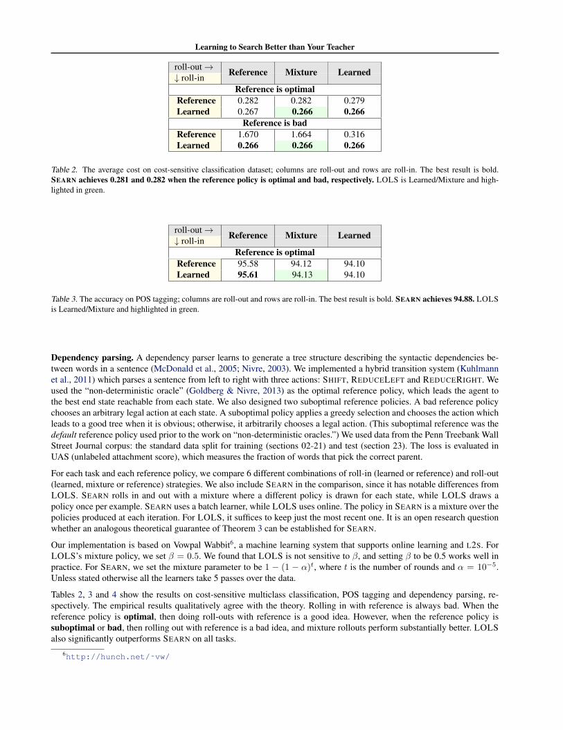
Table 2. The average cost on cost-sensitive classification dataset; columns are roll-out and rows are roll-in. The best result is bold.SEARN achieves 0.281 and 0.282 when the reference policy is optimal and bad, respectively. LOLS is Learned/Mixture and high-lighted in green.



Table 3. The accuracy on POS tagging; columns are roll-out and rows are roll-in. The best result is bold. SEARN achieves 94.88. LOLSis Learned/Mixture and highlighted in green.

Dependency parsing. A dependency parser learns to generate a tree structure describing the syntactic dependencies be-tween words in a sentence (McDonald et al., 2005; Nivre, 2003). We implemented a hybrid transition system (Kuhlmannet al., 2011) which parses a sentence from left to right with three actions: SHIFT, REDUCELEFT and REDUCERIGHT. Weused the “non-deterministic oracle” (Goldberg & Nivre, 2013) as the optimal reference policy, which leads the agent tothe best end state reachable from each state. We also designed two suboptimal reference policies. A bad reference policychooses an arbitrary legal action at each state. A suboptimal policy applies a greedy selection and chooses the action whichleads to a good tree when it is obvious; otherwise, it arbitrarily chooses a legal action. (This suboptimal reference was thedefault reference policy used prior to the work on “non-deterministic oracles.”) We used data from the Penn Treebank WallStreet Journal corpus: the standard data split for training (sections 02-21) and test (section 23). The loss is evaluated inUAS (unlabeled attachment score), which measures the fraction of words that pick the correct parent.

For each task and each reference policy, we compare 6 different combinations of roll-in (learned or reference) and roll-out(learned, mixture or reference) strategies. We also include SEARN in the comparison, since it has notable differences fromLOLS. SEARN rolls in and out with a mixture where a different policy is drawn for each state, while LOLS draws apolicy once per example. SEARN uses a batch learner, while LOLS uses online. The policy in SEARN is a mixture over thepolicies produced at each iteration. For LOLS, it suffices to keep just the most recent one. It is an open research questionwhether an analogous theoretical guarantee of Theorem 3 can be established for SEARN.

Our implementation is based on Vowpal Wabbit6, a machine learning system that supports online learning and L2S. ForLOLS’s mixture policy, we set β = 0.5. We found that LOLS is not sensitive to β, and setting β to be 0.5 works well inpractice. For SEARN, we set the mixture parameter to be 1 − (1 − α)t, where t is the number of rounds and α = 10−5.Unless stated otherwise all the learners take 5 passes over the data.

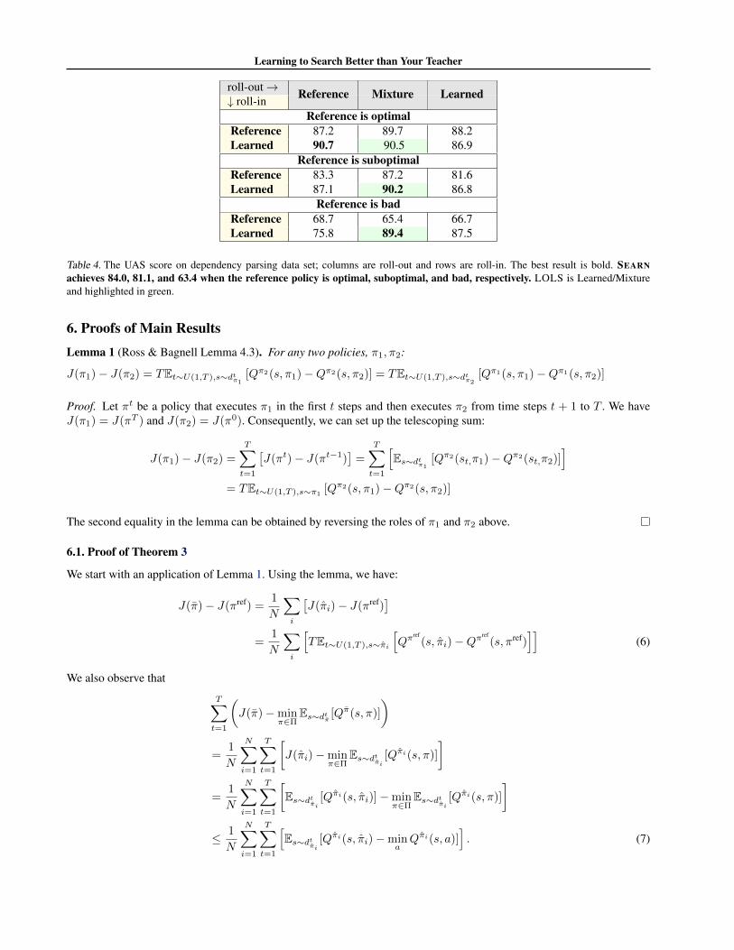
Tables 2, 3 and 4 show the results on cost-sensitive multiclass classification, POS tagging and dependency parsing, re-spectively. The empirical results qualitatively agree with the theory. Rolling in with reference is always bad. When thereference policy is optimal, then doing roll-outs with reference is a good idea. However, when the reference policy issuboptimal or bad, then rolling out with reference is a bad idea, and mixture rollouts perform substantially better. LOLSalso significantly outperforms SEARN on all tasks.

6http://hunch.net/˜vw/

http://hunch.net/~vw/




Reference is suboptimalReference 83.3 87.2 81.6Learned 87.1 90.2 86.8

Reference is badReference 68.7 65.4 66.7Learned 75.8 89.4 87.5

Table 4. The UAS score on dependency parsing data set; columns are roll-out and rows are roll-in. The best result is bold. SEARNachieves 84.0, 81.1, and 63.4 when the reference policy is optimal, suboptimal, and bad, respectively. LOLS is Learned/Mixtureand highlighted in green.

6. Proofs of Main ResultsLemma 1 (Ross & Bagnell Lemma 4.3). For any two policies, π1, π2:

J(π1)− J(π2) = TEt∼U(1,T ),s∼dtπ1[Qπ2(s, π1)−Qπ2(s, π2)] = TEt∼U(1,T ),s∼dtπ2

[Qπ1(s, π1)−Qπ1(s, π2)]

Proof. Let πt be a policy that executes π1 in the first t steps and then executes π2 from time steps t + 1 to T . We haveJ(π1) = J(πT ) and J(π2) = J(π0). Consequently, we can set up the telescoping sum:

J(π1)− J(π2) =

T∑t=1

[J(πt)− J(πt−1)

]=

T∑t=1

[Es∼dtπ1

[Qπ2(st,π1)−Qπ2(st,π2)]]

= TEt∼U(1,T ),s∼π1[Qπ2(s, π1)−Qπ2(s, π2)]

The second equality in the lemma can be obtained by reversing the roles of π1 and π2 above.

6.1. Proof of Theorem 3

We start with an application of Lemma 1. Using the lemma, we have:

J(π)− J(πref) =1

N

∑i

[J(πi)− J(πref)

]=

1

N

∑i

[TEt∼U(1,T ),s∼πi

[Qπ

ref(s, πi)−Qπ

ref(s, πref)

]](6)

We also observe that

T∑t=1

(J(π)−min


)

=1

N

N∑i=1

T∑t=1

[J(πi)−min

π∈ΠEs∼dtπi [Q

πi(s, π)]

]

=1

N

N∑i=1

T∑t=1

[Es∼dtπi [Q

πi(s, πi)]−minπ∈Π

Es∼dtπi [Qπi(s, π)]

]

≤ 1

N

N∑i=1

T∑t=1

[Es∼dtπi [Q

πi(s, πi)−minaQπi(s, a)]

]. (7)


Combining the above bounds from Equations 6 and 7, we see that

β(J(π)− J(πref)

)+ (1− β)

T∑t=1

(J(π)−min


)

≤ 1

N

N∑i=1

T∑t=1

Es∼dtπi

[β(Qπ

ref(s, πi)−Qπ

ref(s, πref)

)+ (1− β)

(Qπi(s, πi)−min

aQπi(s, a)

)]=

1

N

N∑i=1

T∑t=1

Es∼dtπi

[Qπ

outi (s, πi)− βQπ

ref(s, πref)− (1− β) min

aQπi(s, a)

]≤ 1

N

N∑i=1

T∑t=1

Es∼dtπi

[Qπ

outi (s, πi)− βmin

aQπ

ref(s, a)− (1− β) min

aQπi(s, a)

]

6.2. Proof of Corollary 1

The proof is fairly straightforward from definitions. By definition of no-regret, it is immediate that the gap

N∑i=1

T∑t=1

E [ci,t(πi(st))− ci,t(π(st))] = o(NT ), (8)

for all policies π ∈ Π, where we recall that ci,t is the cost-vector over the actions on round i when we do roll-outs from thetth decision point. Let Ei denote the conditional expectation on round i, conditioned on the previous rounds in Algorithm 1.Then it is easily seen that

Ei[ci,t(a)] = Ei[`(ei,t(a))−min

a′`(ei,t(a

′))

],

with ei,t being the end-state reached on completing the roll-out with the policy πouti on round i, when action a was taken

on the decision point t. Recalling that we rolled in following the trajectory of πini , this expectation further simplifies to

Ei[ci,t(a)] = Es∼dtπi

[Qπ

outi (s, a)

]− Ei

[mina′

`(ei,t(a′))

].

Now taking expectations in Equation 8 and combining with the above observation, we obtain that for any policy π ∈ Π,

N∑i=1

T∑t=1

E [ci,t(πi(st))− ci,t(π(st))]

=

N∑i=1

T∑t=1

Es∼dtπi

[Qπ

outi (s, πi(s))−Qπ

outi (s, π(s))

]= o(NT ).

Taking the best policy π ∈ Π and dividing through by NT completes the proof.

6.3. Proof sketch of Theorem 5

(Sketch only) We decompose the analysis over exploration and exploitation rounds. For the exploration rounds, we boundthe regret by its maximum possible value of 1. To control the regret on the exploitation rounds, we focus on the updatesperformed during exploration.

The cost vector c(a) used at an exploration round i satisfies

Ei[c(a)] = Ei [K`(e(at))1[a = at]]

= Et∼U(0:T−1),s∼dtπni

[Qπ

outi (s, a)

],


Corollary 1. Since the cost vector is identical in expectation as that used in Algorithm 1, the proof of theorem 3, which onlydepends on expectations, can be reused to prove a result similar to theorem 3 for the exploration rounds. That is, letting πito be the averaged policy over all the policies in I at exploration round i, we have the bound

β(J(πi)− J(πref)) + (1− β)

T∑t=1

(J(π)−min


)≤ Tδi,

where δi is as defined in Equation 4.

On the exploitation rounds, we can now invoke this guarantee. Recalling that we have ni exploration rounds until round i,the expected regret at an exploitation round i is at most δni . Thus the overall regret of the algorithm is at most

Regret ≤ ε+1

N

N∑i=1

δni ,

which completes the proof.

6.4. Proof of corollary 2

We start by substituting Equation 5 in the regret bound of Theorem 5. This yields

Regret ≤ ε+T

Nδclass +

cKT

N

N∑i=1

√log |Π|ni

.

We would like to further replace ni with its expectation which is εi. However, this does not yield a valid upper bounddirectly. Instead, we apply a Chernoff bound to the quantity ni, which is a sum of i i.i.d. Bernoulli random variables withmean ε. Consequently, we have

P (ni ≤ (1− γ)εi) ≤ exp

(−γ

2εi

2

)≤ exp(−εi/8),

for γ = 1/2. Let i0 = 16 logN/ε+ 1. Then we can sum the failure probabilities above for all i ≥ i0 and obtain

N∑i=i0

P (ni ≤ εi/2) ≤N∑i=i0

exp(−εi/8) ≤∞∑i=i0

exp(−εi/8)

≤ exp(−εi0/8)

1− exp(−ε/8)

=exp(−2 logN)

exp(ε/8)− 1≤ 8

N2ε,

where the last inequality uses 1 + x ≤ exp(x). Consequently, we can now allow a regret of 1 on the first i0 rounds, andcontrol the regret on the remaining rounds using ni ≤ εi/2. Doing so, we see that with probability at least 1− 2/(N2ε)

Regret ≤ ε+i0N

+T

Nδclass +

cKT

N

N∑i=1

√2 log |Π|

εi

≤ ε+16 logN + ε

Nε+T

Nδclass +

8cKT log |Π|εN

Choosing ε = (KT )2/3(log(N |Π|)/N)1/3 completes the proof.

6.5. Proof of Theorem 4

The proof follows from results in combinatorics. The dynamics of algorithms considered here can be thought of as a paththrough a graph where the vertices are the corners of the boolean hypercube in T dimensions with two vertices at Hamming


1

10

0

0 0 0 0

01

1 1 1 1

111

000

001 010 100

011 101 110

111

000

001 010 100

011 101 110

111

000

001 010 100

011 101 110

(a) (b) (c) (d)

Figure 4. Pictorial illustration of the proof elements of Theorem 4. Panel (a) depicts the actions chosen by policy 000. Selected action ineach state is indicated in bold. Panels (b) through (d) depict various stages as the algorithm updates the policy to its one-step deviations,starting from the policy 000. Each policy that the algorithm selects is depicted by a shaded circle, with the arrows marking the movesof the algorithm. Current policy is the shaded circle with a bold boundary. Dashed lines denote the potential one-step deviations that thealgorithm can move to and crossed policies are those which have higher costs than the current policy (see text for details).

distance 1 sharing an edge. We demonstrate that there is a cost function such that the algorithm is forced to traverse a longpath before reaching a local optimum. Without loss of generality, assume that the algorithm always moves to a one-stepdeviation with the lowest cost since otherwise longer paths exist.

To gain some intuition, first consider T = 3 which is depicted in Figure 4. Suppose the algorithm starts from the policy000 then moves to the policy 001. If the algorithm picks the best amongst the one-step deviations, we know that J(001) ≤minJ(000), J(010), J(100), placing constraints on the costs of these policies which force the algorithm to not visit anyof these policies later. Similarly, if the algorithm moves to the policy 011 next, we obtain a further constraint J(011) <minJ(101), J(001). It is easy to check that the only feasible move (corresponding to policies not crossed in Figure 4(c))which decreases the cost under these constraints is to the policy 111 and then 110, at which point the algorithm attainslocal optimality since no more moves that decrease the cost are possible. In general, at any step i of the path, the policyπi is a one-step deviation of πi−1 and at least 2 or more steps away from πj for j < i − 1. The policy never moves to aneighbor of an ancestor (excluding the immediate parent) in the path.

This property is the key element to understand more generally. Suppose we have a current path π1 → π2 . . .→ πi−1 → πi.Since we picked the best neighbor of πj as πj+1, πi+1 cannot be a neighbor of any πj for j < i. Consequently, themaximum number of updates the algorithm must make is given by the length of the longest such path on a hypercube,where each vertex (other than start and end) neighbors exactly two other vertices on the path. This is called the snake-in-the-box problem in combinatorics, and arises in the study of error correcting codes. It is shown by Abbott & Katchalski(1988) that the length of longest such path is Θ(2T ). With monotonically decreasing costs for policies in the path andmaximal cost for all policies not in the path, the traversal time is Θ(2T ).

Finally, it might appear that Algorithm 1 is capable of moving to policies which are not just one-step deviations of thecurrently learned policy, since it performs updates on “mini-batches” of T cost-sensitive examples. However, on this lowerbound instance, Algorithm 1 will be forced to follow one-step deviations only due to the structure of the cost function. Forinstance, from the policy 000 when we assign maximal cost to policies 010 and 100 in our example, this corresponds tomaking the cost of taking action 1 on first and second step very large in the induced cost-sensitive problem. Consequently,001 is the policy which minimizes the cost-sensitive loss even when all the T roll-outs are accumulated, implying thealgorithm is forced to traverse the same long path to local optimality.

AcknowledgementsPart of this work was carried out while Kai-Wei, Akshay and Hal were visiting Microsoft Research.

ReferencesAbbott, H.L and Katchalski, M. On the snake in the box problem. Journal of Combinatorial Theory, Series B, 45(1):13 –

24, 1988.

Cesa-Bianchi, N. and Lugosi, G. Prediction, Learning, and Games. Cambridge University Press, 2006.

Collins, Michael and Roark, Brian. Incremental parsing with the perceptron algorithm. In Proceedings of the Conference


of the Association for Computational Linguistics (ACL), 2004.

Daume III, Hal and Marcu, Daniel. Learning as search optimization: Approximate large margin methods for structuredprediction. In Proceedings of the International Conference on Machine Learning (ICML), 2005.

Daume III, Hal, Langford, John, and Marcu, Daniel. Search-based structured prediction. Machine Learning Journal, 2009.

Daume III, Hal, Langford, John, and Ross, Stephane. Efficient programmable learning to search. arXiv:1406.1837, 2014.

Doppa, Janardhan Rao, Fern, Alan, and Tadepalli, Prasad. HC-Search: A learning framework for search-based structuredprediction. Journal of Artificial Intelligence Research (JAIR), 50, 2014.

Goldberg, Yoav and Nivre, Joakim. Training deterministic parsers with non-deterministic oracles. Transactions of theACL, 1, 2013.

Goldberg, Yoav, Sartorio, Francesco, and Satta, Giorgio. A tabular method for dynamic oracles in transition-based parsing.Transactions of the ACL, 2, 2014.

He, He, Daume III, Hal, and Eisner, Jason. Imitation learning by coaching. In Neural Information Processing Systems(NIPS), 2012.

Kuhlmann, Marco, Gomez-Rodrıguez, Carlos, and Satta, Giorgio. Dynamic programming algorithms for transition-baseddependency parsers. In Proceedings of the 49th Annual Meeting of the Association for Computational Linguistics:Human Language Technologies-Volume 1, pp. 673–682. Association for Computational Linguistics, 2011.

Langford, John and Beygelzimer, Alina. Sensitive error correcting output codes. In Learning Theory, pp. 158–172.Springer, 2005.

Marcus, Mitch, Marcinkiewicz, Mary Ann, and Santorini, Beatrice. Building a large annotated corpus of English: ThePenn Treebank. Computational Linguistics, 19(2):313–330, 1993.

McDonald, Ryan, Pereira, Fernando, Ribarov, Kiril, and Hajic, Jan. Non-projective dependency parsing using spanningtree algorithms. In Proceedings of the Joint Conference on Human Language Technology Conference and EmpiricalMethods in Natural Language Processing (HLT/EMNLP), 2005.

Nivre, Joakim. An efficient algorithm for projective dependency parsing. In International Workshop on Parsing Technolo-gies (IWPT), pp. 149–160, 2003.

Ross, Stephane and Bagnell, J. Andrew. Efficient reductions for imitation learning. In Proceedings of the Workshop onArtificial Intelligence and Statistics (AI-Stats), 2010.

Ross, Stephane and Bagnell, J. Andrew. Reinforcement and imitation learning via interactive no-regret learning.arXiv:1406.5979, 2014.

Ross, Stephane, Gordon, Geoff J., and Bagnell, J. Andrew. A reduction of imitation learning and structured prediction tono-regret online learning. In Proceedings of the Workshop on Artificial Intelligence and Statistics (AI-Stats), 2011.

Zinkevich, Martin. Online convex programming and generalized infinitesimal gradient ascent. In Proceedings of theInternational Conference on Machine Learning (ICML), 2003.


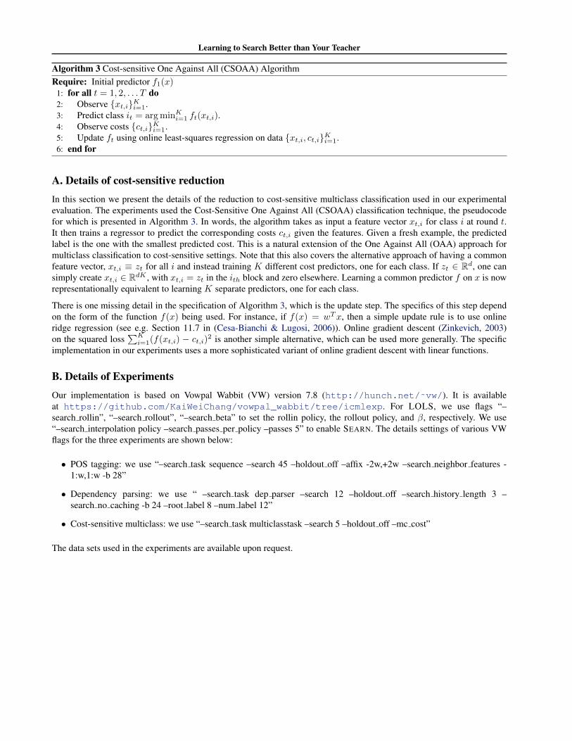
Algorithm 3 Cost-sensitive One Against All (CSOAA) AlgorithmRequire: Initial predictor f1(x)

1: for all t = 1, 2, . . . T do2: Observe xt,iKi=1.3: Predict class it = arg minKi=1 ft(xt,i).4: Observe costs ct,iKi=1.5: Update ft using online least-squares regression on data xt,i, ct,iKi=1.6: end for

A. Details of cost-sensitive reductionIn this section we present the details of the reduction to cost-sensitive multiclass classification used in our experimentalevaluation. The experiments used the Cost-Sensitive One Against All (CSOAA) classification technique, the pseudocodefor which is presented in Algorithm 3. In words, the algorithm takes as input a feature vector xt,i for class i at round t.It then trains a regressor to predict the corresponding costs ct,i given the features. Given a fresh example, the predictedlabel is the one with the smallest predicted cost. This is a natural extension of the One Against All (OAA) approach formulticlass classification to cost-sensitive settings. Note that this also covers the alternative approach of having a commonfeature vector, xt,i ≡ zt for all i and instead training K different cost predictors, one for each class. If zt ∈ Rd, one cansimply create xt,i ∈ RdK , with xt,i = zt in the ith block and zero elsewhere. Learning a common predictor f on x is nowrepresentationally equivalent to learning K separate predictors, one for each class.

There is one missing detail in the specification of Algorithm 3, which is the update step. The specifics of this step dependon the form of the function f(x) being used. For instance, if f(x) = wTx, then a simple update rule is to use onlineridge regression (see e.g. Section 11.7 in (Cesa-Bianchi & Lugosi, 2006)). Online gradient descent (Zinkevich, 2003)on the squared loss

∑Ki=1(f(xt,i) − ct,i)2 is another simple alternative, which can be used more generally. The specific

implementation in our experiments uses a more sophisticated variant of online gradient descent with linear functions.

B. Details of ExperimentsOur implementation is based on Vowpal Wabbit (VW) version 7.8 (http://hunch.net/˜vw/). It is availableat https://github.com/KaiWeiChang/vowpal_wabbit/tree/icmlexp. For LOLS, we use flags “–search rollin”, “–search rollout”, “–search beta” to set the rollin policy, the rollout policy, and β, respectively. We use“–search interpolation policy –search passes per policy –passes 5” to enable SEARN. The details settings of various VWflags for the three experiments are shown below:

• POS tagging: we use “–search task sequence –search 45 –holdout off –affix -2w,+2w –search neighbor features -1:w,1:w -b 28”

• Dependency parsing: we use “ –search task dep parser –search 12 –holdout off –search history length 3 –search no caching -b 24 –root label 8 –num label 12”

• Cost-sensitive multiclass: we use “–search task multiclasstask –search 5 –holdout off –mc cost”

The data sets used in the experiments are available upon request.

http://hunch.net/~vw/

https://github.com/KaiWeiChang/vowpal_wabbit/tree/icmlexp

Documents

Learning to Search Better than Your TeacherLearning to Search Better than Your Teacher)=0.2y y y x Î X e Î Y, l(y e)=0.0 e Î Y, l(y e e Î Y, l(y e)=0.8 Figure 2. An example search