Learning Through Noticing: Theory and

Experimental Evidence in Farming∗

Rema Hanna

Harvard University, NBER and BREAD

Sendhil Mullainathan

Harvard University and BREAD

Joshua Schwartzstein

Dartmouth College

April 18, 2014

Abstract

We consider a model of technological learning under which people “learn through noticing”:they choose which input dimensions to attend to and subsequently learn about from availabledata. Using this model, we show how people with a great deal of experience may persistentlybe off the production frontier because they fail to notice important features of the data that theypossess. We also develop predictions on when these learning failures are likely to occur, aswell as on the types of interventions that can help people learn. We test the model’s predictionsin a field experiment with seaweed farmers. The survey data reveal that these farmers do notattend to pod size, a particular input dimension. Experimental trials suggest that farmers areparticularly far from optimizing this dimension. Furthermore, consistent with the model, wefind that simply having access to the experimental data does not induce learning. Instead,behavioral changes occur only after the farmers are presented with summaries that highlightpreviously unattended-to relationships in the data. JEL codes: D03, D83, O13, O14, O30, Q16

∗We thank Daniel Benjamin, Matthew Gentzkow, Marina Halac, Andy Newman, Ted O’Donoghue, Tim Og-den, Matthew Rabin, Andrei Shleifer, and four anonymous referees for extremely helpful comments, as well asseminar participants at the Behavioural Decision Theory Conference, Berkeley, BREAD, BU, Chicago Booth,Cornell, Duke, Harvard/MIT, the NBER Organizational Economics Meeting, and SITE. We thank the Interna-tional Finance Corporation for financial support. E-mail: rema_hanna@ksg.harvard.edu, mullain@fas.harvard.edu,josh.schwartzstein@dartmouth.edu.

1

1 Introduction

Many production functions are not known ex ante. Instead, they are learned, both from personal

experiences (Gittins 1979; Arrow 1962; Jovanovic and Nyarko 1996; Foster and Rosenzweig 1995)

and from those of others (Besley and Case 1993, 1994; Banerjee 1992; Bikhchandani et al. 1992;

Munshi 2004; Conley and Udry 2010). While diverse, existing learning models share a common

assumption: the key input for learning is informative data.

Many examples, however, defy this assumption. For many years, doctors had the data that

they needed to prevent operating room infections, but the importance of a sterile operating room

was not recognized until the germ theory of disease was accepted (Nuland 2004; Gawande 2004).

Indian textile manufacturers failed to adopt key management practices, such as having an unclut-

tered factory floor, despite exposure to natural variation that pointed to their importance (Bloom et

al. 2013). Even experienced teachers do not adopt the best teaching practices (Allen et al. 2011).

These examples all imply that learning is not just about the data that you possess, but what you

notice in those data. In fact, we may not learn from the data that we ourselves generate.

In this paper, we use Schwartzstein’s (2014) model of selective attention to build a model

of learning through noticing and test its predictions in a field experiment with seaweed farmers.1

The model highlights an important constraint on learning. A farmer planting a crop faces a slew

of potential features that might affect production – crop spacing, the time of planting, the amount

and timing of the water employed, the pressure of the soil on the seedlings, and so on. He cannot

possibly attend to everything (Kahneman 1973): his attention is limited (or effortful), while the

number of potentially important variables is large. Since he can only learn about the dimensions

that he notices (or attends to), this choice becomes a key input into the learning process.

In the model, the farmer allocates attention in a “Savage rational” way: he optimally chooses

1While the model presented in this paper is specific to issues related to technological use, Schwartzstein (2014)presents a general model of belief formation when agents are selectively attentive. The approach of modeling economicagents as responding only to a subset of available information dates back to at least Simon (1955). Nelson and Winter(1982) consider how bounded rationality (or “evolutionary processes”) impact technological change. For more recentapproaches to modeling limited attention in economic settings, see Sims (2003), Bordalo et al. (2012, 2013), Koszegiand Szeidl (2013), and Gabaix (2013).

2

what to attend to as a Bayesian, given his prior beliefs and the costs of paying attention. Consistent

with the above examples, even with substantial experience – and even with lots of readily available

data – a farmer may not approach the productivity frontier. Despite the (subjective) optimality as-

sumption, an interesting feedback loop arises: a farmer who initally believes that a truly important

dimension is unlikely to matter will not attend to it, and consequently will not learn whether it does

matter. This failure to learn stems from not focusing on aspects of the data that could contradict

a false belief. When the technology is incongruent with the farmer’s priors, the losses from such

sub-optimization can be arbitrarily large.

While other models of incomplete learning also accommodate the idea that people can persis-

tently be far from the productivity frontier, our model predicts where these failures should occur.

Learning failures should be concentrated on dimensions where the agents report ignorance, i.e.,

where they cannot answer key questions about what they precisely do (or have done) along those

dimensions. Most other theories of mis-optimization (arising from over-confidence, false beliefs,

unawareness, etc.) have little to say about this “failure to notice” variable.

To test the model’s predictions, we conducted a field experiment with seaweed farmers in

Indonesia. Seaweed is farmed by attaching strands (“pods”) to lines submerged in the ocean. As

in the model, a large number of dimensions affect yield. To look for failures to notice, we directly

asked farmers about their own production techniques. Farmers are quite knowledgeable and have

clear opinions about many dimensions: almost all farmers had an opinion about the length of their

typical line, the typical distance between their lines, the optimal distance between their knots (i.e.,

pods), the optimal distance between lines, and the optimal cycle length. On the other hand, most

do not recognize a role for one key dimension: about 85 percent do not know the size of their pods

and will not venture a guess about what the optimal size might be.2

To test whether this apparent failure to notice translates into a learning failure, we conducted

experiments on the farmers’ own plots, varying both pod size and pod (or “knot”) spacing. On pod

2Many other dimensions might be important: For example, the strength of the tide, the time of day, the temperature,the tightness with which pods are attached, the strain of pods used, etc. could matter. In our analysis, we largely focuson two or three dimensions for parsimony, but actual demands on attention are much greater.

3

spacing, which almost all farmers had an opinion about, our findings suggest that they were close

to the optimum. In contrast, on pod size – which few farmers had an opinion about – our findings

suggest they were far from it.

Further support for the model comes from examining farmers’ response to the trial. The

model suggests that simply participating in the trials may not change the farmers’ behavior with

respect to pod size.3 Intuitively, the farmers’ own inattentive behavior generates an experiment of

sorts every season – random variation in pod sizing – and the trial presents farmers with similar

data that they already had access to, but did not learn from. Consistent with this idea, we find little

change in pod size following participation in the trial. However, the model suggests an alternative

way to induce learning: to provide a summary of the data that explicitly highlights neglected rela-

tionships. Consistent with this prediction, we find that farmers changed their production methods

after we presented them with the trial data on yield broken down by pod size from their own plots.

Beyond the analysis of seaweed farming, we extend the model to illustrate how greater ex-

perience with related technologies can predictably increase the likelihood of learning failures and

make precise a notion of “complexity” of the current technology that can also induce failures.

The potential costs of experience and the role of complexity are consistent with folk wisdom and

evidence on technology adoption and use (e.g., Rogers 2003), but to our knowledge have largely

remained theoretically unexplored.

The model also has broader implications for understanding which types of interventions can

help individuals learn. In most learning models, providing more data induces learning. Our model

and experimental results, in contrast, suggest that simply providing more data can have little impact

on behavior if data availability is not a first order problem. Our findings shed light on why some

agricultural extension activities are ineffective, or only moderately effective in the long run (e.g.,

Kilby 1962; Leibenstein 1966; Duflo, Kremer and Robinson 2008b). At the opposite extreme, our

3Strictly speaking, this is a prediction of the model under the assumption that merely being asked to participatedoes not, by itself, significantly alter farmers’ beliefs about the importance of pod size, which we had prior reasonto believe would be true (as we discuss below). It also relies on an assumption that it is not significantly easier forthe farmers to learn relationships from the raw trial data than from the data they are typically exposed to, which alsoseems plausible given the experimental design.

4

model and experimental results show how one can induce learning without providing new data

by simply providing summaries highlighting previously unattended-to relationships in the agents’

own data. This result aligns with growing evidence that interventions that encourage agents to

attend more closely to available data can profitably impact behavior in diverse contexts ranging

from car manufacturing (Liker 2004), to teaching (Allen et al. 2011), to shopkeeping (Beaman,

Magruder, and Robinson 2014).

The paper proceeds as follows. Section 2 presents the baseline model of learning through

noticing and develops the empirical predictions. Section 3 describes the experiment, while Section

4 provides its results. Section 5 explores other potential applications and extends the model to

develop comparative static predictions on the prevelance of failures to notice and resulting failures

to learn. Section 6 concludes.

2 Model

2.1 Setup

We present a stylized model of learning through noticing. We present it for the case of a farmer

to make it concrete, but reinterpret it for other contexts, such as management or education, in

Section 5. A farmer plants the same crop for two periods, t ∈ {1,2}. He works on a continuous

sets of plots indexed by l ∈ [0,1]. To capture the idea that the constraint on learning comes from

having many things to pay attention to, his production technology has many dimensions that might

matter. Specifically, for each of his plots l, the farmer chooses an N-dimensional vector of inputs,

x = (x1,x2, . . .xN), where each x j is drawn from a finite set X j, and where we denote the set of

possible x by X .

Given the input bundle x ∈ X , the dollar value of net yield (total yield net of the costs of

5

inputs) for the farmer from a plot l at time t is:

ylt = f (x|θ)+ εlt =N

∑j=1

f j(x j|θ j)+ εlt , (1)

where θ = (θ1, . . . ,θN) is some fixed parameter of the technology (described below) and εlt ∼

N (0,σ2ε ) is a mean zero shock that is independent across plots of land and time.4

2.1.1 Beliefs

Since the model focuses on how inattention impacts learning, we assume that the farmer initially

does not know the parameters of the production function: he must learn θ = (θ1, . . . ,θN) through

experience.

The farmer begins with some prior beliefs about θ , where we denote a generic value by

θ . We assume that while many dimensions could be relevant for production, only a few of them

actually are. To capture this, we assume that the farmer attaches prior weight π j ∈ (0,1) to input

j being relevant and the remaining weight, (1−π j), to input j being irrelevant. Specifically, the

farmer’s prior holds that:

f j(x j|θ j) =

0 if input j is irrelevant

θ j(x j)∼N (0,ν2), i.i.d across x j ∈ X j if input j is relevant.(2)

We assume ν2 > 0 and that the prior uncertainty is independent across dimensions, meaning that

knowledge of how to set input j does not help the farmer set input j′. Under these assumptions,

when input j is irrelevant, it does not matter how x j is set. When input j is relevant, with probability

one some particular level of x j produces the greatest output. But the farmer does not initially know

which one because the exact θ j is unknown and must be learned.

4Note that l and t appear symmetrically in Equation (1). For the purpose of forming beliefs about the underlyingtechnology (θ ), it does not matter whether the farmer learns through many observations across plots at a fixed time,or through many observations over time on a fixed plot. Equation (1) also reflects a simplifying assumption that thepayoff function is separable across input dimensions, allowing us to separately analyze the farmer’s decisions acrossdimensions.

6

2.1.2 Costly Attention

To this standard learning problem, we add limited attention. The farmer makes a zero-one decision

of whether or not to attend to a given input. Let at ∈ {0,1}N denote a vector that encodes which

dimensions the farmer attends to in period t, where a jt = 1 if and only if he attends to dimension j

in period t. For each input dimension he attends to, he faces a cost e, reflecting the shadow cost of

mental energy and time.

Inattention operates in two ways. First, when the farmer does not attend to input j, a “default

action” is taken, which we capture simply as a uniform distribution over the possible values of

that input: X j. Thus, the farmer’s actions are random in the absence of attention. When a farmer

attends to an input, he chooses its level.

Second, if the farmer does not attend to an input, he also does not notice the set level(s). Thus,

in period 2, instead of knowing the values x jl1 which were actually chosen, he only remembers:

x jl1 =

x jl1 if a j1 = 1

∅ if a j1 = 0.(3)

Notationally, we write the full second-period history as h = (yl1,xl1)l∈[0,1], which is what the

farmer would recall if he were perfectly attentive, and h = (yl1, xl1)l∈[0,1], as the recalled history.5

In our seaweed application, if the farmer does not attend to pod size, he both creates random

variation by virtue of not focusing on this dimension when cutting raw seaweed into pods and

does not know the know the specific pod sizes that were set, making it harder for him to learn a

relationship between pod size and output.

5Under the interpretation that y measures the dollar value of yield net of input costs, we are implicitly assumingthat the farmer knows the total input costs even if he does not attend to certain input choices. By analogy, we mayknow our total monthly spending without knowing our spending by category, e.g., food or clothing.

7

2.1.3 The Farmer’s Problem

The farmer is risk-neutral and maximizes the expected undiscounted sum of net payoffs – yield

minus attentional costs – across the two periods. To simplify the presentation by allowing us to

drop the l subscript, we restrict the farmer to strategies that are symmetric across plots in a given

period, but allow him to mix over input choices. When it does not cause confusion, we abuse

notation and let x jt both denote the farmer’s choice along dimension j at time t if he attends to that

input, and the default uniform distribution over possible input levels when he does not attend.

This simple model captures a basic learning problem. In the first period, the farmer makes

choices that trade off the future benefits of experimentation against maximizing current expected

payoffs. In the second period, the farmer simply chooses to maximize current expected payoffs.6

2.2 Results

We first ask when the farmer will end up at the productivity frontier. For a technology (θ ) and

given cost of attention (e), let x∗j denote a (statically) optimal input choice along dimension j.

More precisely, x∗j maximizes f j(x j|θ j) whenever dimension j is worth attending to, i.e., whenever

the payoff from setting the optimal input along dimension j and incurring the attentional cost to

do so, maxx j f j(x j|θ j)− e, exceeds the payoff from not attending to the input and thus randomly

setting it, 1|X j|∑x′j

f j(x′j|θ j). Whenever dimension j is not worth attending to, x∗j equals the default

uniform distribution over X j (with an obvious abuse of notation). To make the problem interesting,

we assume that there is at least one dimension that is worth paying attention to, as otherwise the

farmer will necessarily end up at the frontier.

To more broadly understand when the farmer ends up at the productivity frontier, we focus

on second period choices.

6The model’s assumption of two periods, but many plots, implies that experimentation will occur across plotsin a fixed time period, rather than over time. Thus, we can avoid tangential issues that arise in settings with multi-period experimentation, such as considering the degree to which agents are sophisticated in updating given missinginformation (Schwartzstein 2014). That there are a continuum of plots also simplifies matters by allowing us to abstractfrom noise in the learning process; the farmer can in principle perfectly learn the technology in a single period. Thiswill allow us to focus on how inattention, rather than incomplete information, contributes to incomplete learning.

8

Proposition 1.

1. When there are no costs of attention (e = 0), the farmer learns to optimize every dimension:

in the second (terminal) period he chooses x j2 = x∗j for all j.

2. With costs of attention (e > 0),

(a) The farmer may not learn to optimize certain dimensions: For every technology θ ,

there exists a collection of prior weights πi > 0, i = 1 . . . ,N, such that in the second

period he chooses x j2 6= x∗j for some input j.

(b) Losses from not optimizing are unboundedly large: For every constant K ∈ R+, there

exists a technology θ and collection of prior weights πi > 0, i = 1 . . . ,N, such that in

the second period the farmer chooses x j2 6= x∗j for some j and, by doing so, loses at

least K.

3. The farmer does not learn to optimize a dimension only if he did not attend to it in the first

period: in the second period he chooses x j2 6= x∗j only if a j1 = 0.

Proof. See Online Appendix A for all proofs. �

The first part of Proposition 1 replicates the standard result of learning by doing models that,

with no costs of attention, learning is primarily a function of experience and enough of it guar-

antees optimal technology use (e.g., Arrow 1962; Nelson and Phelps 1966; Schultz 1975). This

intuition is invoked – at least implicitly – in arguments that learning by doing is not an impor-

tant determinant of adoption for old technologies in which individuals have abundant experience

(Foster and Rosenzweig 2010).

The second part of the proposition in contrast shows that, with costs of attention, failures to

notice can lead to failures to learn and these failures can lead to arbitrarily large payoff losses. The

basic idea is simple: inattention is self-confirming (Schwartzstein 2014). If the farmer initially

falsely believes an input is not worth attending to, he will not notice the information that proves

9

him wrong and will continue not attending to the input even if it is very important.7 As the proof

of Proposition 1 makes clear, the farmer fails to learn to optimize dimension j when the dimension

matters, but he places sufficiently low prior weight π j on it mattering. Resulting errors can be

arbitrarily large: the constant K need not be in any way proportional to the cost of attention,

so even very small attentional costs can produce large losses. The final part of the proposition

says that optimization failures come directly from noticing failures in our model. This makes the

model testable by placing an empirically verifiable restriction that a farmer fails to optimize on a

dimension j only if x jl1 =∅ on that dimension.8

Proposition 1 yields the following testable predictions:

Prediction P1 Agents may fail to attend to some dimensions.

Prediction P2 Agents may persistently choose sub-optimal input levels along some dimensions.

Prediction P3 Agents only persistently choose sub-optimal input levels along dimensions they do

not attend to, which can be identified by measuring recall.

To develop further predictions, remember that inattention has two consequences: a failure to

precisely set input levels and a failure to notice and recall what they are. These two effects work in

different directions. Failing to remember clearly impedes learning. However, failing to precisely

set input levels can help learning: when the farmer does not attend to an input, he inadvertently

experiments and generates valuable data. Since he does not notice this data, he does not capitalize

on it. But this distinction has an interesting implication.

Specifically, suppose that in period 2 a farmer could have access to summary statistics about

his own data from period 1, for example because an extension officer calculates and presents the

farmer with such information. What effect would this have? One way to model this is to suppose

that, for each input j, the farmer is told the level x∗j ∈ X j that achieved the greatest yield in period 1,

7The logic is similar to why individuals can maintain incorrect beliefs about the payoff consequences to actionsthat have rarely been tried in bandit problems (Gittins 1979) and in self-confirming equilibria (Fudenberg and Levine1993), and why these incorrect beliefs in turn support sub-optimal decisions.

8Similarly, under the assumption that farmers do not measure and consequently randomly select inputs alongdimensions they do not pay attention to, identifying dimensions along which farmers persistently use a wide variety ofinput levels will also predict failures to notice and resulting failures to learn. Likewise, identifying dimensions alongwhich farmers cannot recall the empirical relationship between the input level and the payoff will predict such failures.

10

as well as the corresponding sample average y j(x∗j).9 Since the cost of tracking the input relative to

yield on measure 1 of plots of land is e, it is natural to assume that the cost of attending to a single

statistic (y j(x∗j), x∗j) is much lower, which for simplicity we will take to equal zero. To emphasize

the impact of receiving a summary about data the farmer would generate on his own, suppose that

receiving it comes as a complete surprise: when choosing how to farm and what to attend to in

the first period he does not anticipate that he will later be provided with this summary. However,

suppose that he understands how the summary is constructed, i.e., that he correctly interprets the

summary given his prior over θ and the objective likelihood function of the summary.

Proposition 2. If the farmer has access to summary information ((y j(x∗j), x∗j)

Nj=1) prior to making

second period decisions, then he learns to optimize every dimension j: he chooses x j2 = x∗j for all

j.

The intuition behind Proposition 2 is simple: together with h, (y j(x∗j), x∗j) is a sufficient

statistic relative to the farmer’s second-period decision along dimension j, i.e., he will make the

same choice on that dimension whether he knows all of h or just h and (y j(x∗j), x∗j).

Proposition 2 demonstrates that, in the model, learning failures do not result from a lack of

readily available data (or from a doctrinaire prior that does not allow for learning), but rather from

a failure to attend to important details of the data.10 Summarizing features of the data that the

farmer had seen but failed to notice can thus be useful.

The value of summaries relies on the farmer facing costs of paying attention and not attending

9Specifically, letting L j(x j) ={

l ∈ [0,1] : x jl1 = x j}

denote the set of plots of land where the farmer uses inputlevel x j in the first period, the sample average payoff conditional on using that input equals:

y j(x j) =1

|L(x j)|

∫l∈L(x j)

yl1dl =1

|L(x j)|

∫l∈L(x j)

f j(x j|θ j)+ ∑k 6= j

fk(xkl1|θk)+ εl1dl

= f j(x j|θ j)+ ∑k 6= j

fk(σk1|θk),

where σk1 ∈ ∆(Xk) denotes the distribution over input levels in Xk implied by the farmer’s first period strategy. x∗j isthen defined as a maximizer of y j(·), where any ties are arbitrarily broken.

10The stark finding of Proposition 2 – that any failure to learn stems solely from failing to extract information fromavailable data, rather than a lack of exposure – relies on the richness of the environment, e.g., that there is a continuumof plots. The key point is more general: Given the data that he generates, the inattentive farmer could benefit fromprocessing those data differently when he did not attend to important input dimensions when forming beliefs.

11

to some dimensions on his own, as Proposition 1 demonstrates that the farmer will otherwise learn

to optimize independent of receiving a summary. In fact, combining the two propositions yields

the simple corollary that the farmer will react to the summary only along dimensions he does not

attend to in its absence. The model may thus rationalize certain extension or consulting activities

that do not help agents collect new data, but rather to record and highlight relationships in those

data. For the purpose of the main empirical exercise, we have the following predictions:

Prediction P4 Agents may fail to optimize along neglected dimensions, even though they are gen-

erating the data that would allow them to optimize.

Prediction P5 Summaries generated from the agents’ own data can change their behavior.

2.3 Comparison with Alternative Approaches

We briefly contrast our model with alternative approaches. First, a model in which an agent exoge-

neously fails to optimize along certain dimensions would be simpler, but would problematically be

consistent with every kind of learning failure. In contrast, our model allows for testable predictions

about when an agent will fail to optimize, for example when he cannot answer questions about what

he does. Second, a more extreme form of not noticing –unawareness– could also produce failures

to learn, where unawareness means that an agent does not even realize that a dimension exists.

Conversely, our model predicts that an agent may persistently fail to optimize along important di-

mensions he is aware of when a technology is prior incongruent– failures to learn come from not

appreciating the importance of variables instead of from neglecting their existence entirely. For

example, in contrast to models of unawareness, doctors were dismissive of practices like hand-

washing long after it was hypothesized that there could be empirical relationships between doctors

washing their hands and outcomes like maternal deaths (Nuland 2004). The germ theory of dis-

ease was important for getting doctors to appreciate such relationships. Third, the predictions of

our model are distinct from those of “bandit models” (Gittins 1979), models of self-confirming

equilibria (Fudenberg and Levine 1993), or “local” models of learning by doing (Conley and Udry

2010). While such models also allow for persistent failures to optimize, in those models a lack of

12

data explains learning failures. When the binding constraint is instead a failure to notice, the main

bottleneck is not one of data collection, but rather data processing.

Finally, models of “rational inattention” (e.g., Sims 2003 or Gabaix 2013) also model atten-

tional costs, but further assume a form of rational expectations in which agents know what is worth

attending to, rather than having to learn what to attend to through experience. This assumption

implies that the size of learning failures resulting from inattention is bound by attentional costs. In

contrast, Proposition 1 shows that potential losses from not noticing are unboundedly large in our

model: our model can shed light on big deviations from optimality.

2.4 Applying the Model

The analysis suggests an exercise with the following steps: (i) find a multi-dimensional setting

with experienced agents, (ii) predict or measure what agents attend to, (iii) assess whether agents

are optimizing, (iv) assess whether agents could achieve a higher payoff given data available to

them, and (v) conduct an “attentional intervention.”

For (i), we prefer a setting in which the first order reason behind any incomplete learning

is compellingly a failure to notice rather than a lack of available information. Situations with

experienced farmers, using mostly old technologies (e.g., fertilizer) fits this description; situations

in which a new technology has just been introduced (e.g., hybrid seeds in the 1920s) may be more

fruitfully analyzed through the lens of more traditional models of technology adoption and use.

For (ii), we would like to collect data that can be used to predict or measure which dimen-

sions of the production process agents do or do not pay attention to, which, when combined with

knowledge of the production function, can be used to predict whether agents are optimizing. Such

data can include survey responses detailing agents’ beliefs about how they have set inputs along

various production dimensions in the past (allowing agents to reveal their knowledge on those in-

puts), their beliefs about what constitutes best practices, and data on how they actually set inputs.

For (iii) and (iv), we want to collect or generate data that can be used to analyze whether

agents are optimizing given data available to them, and whether they do a poorer job optimizing

13

dimensions they appear not to pay attention to. To perform this exercise, Proposition 2 suggests

that it may suffice to analyze data that the agent generates herself.

For (v), we want to perform an intervention that involves presenting information in a way

that helps agents learn relationships that they would not learn on their own, and examine whether

the intervention affects agents’ behavior and resulting payoffs. From Proposition 2, such an in-

tervention can involve providing a summary of how different input choices along unattended-to

dimensions (identified by (ii)) have empirically influenced the payoff-relevant output, given data

agents in principle have available to them.

The seaweed experiment, detailed below, follows the steps laid out above and tests predic-

tions P1-P5. The model generates testable predictions beyond P1-P5 that can be explored by

following additional exercises. Section 5 details some of these predictions and exercises.

3 The Seaweed Experiment

3.1 Setting

Our experiment takes place with seaweed farmers in the Nusa Penida district in Indonesia. Sea-

weed farming exhibits key features of an ideal setting discussed in Section 2.4: it involves experi-

enced agents who have had many opportunities to learn – they have grown seaweed since the early

1980s, with many crop cycles in each year – but where the production technology involves many

dimensions.

Most farmers in the area that we study follow what is called “the bottom method”: in each

plot, a farmer drives wooden stakes in the shallow bottom of the ocean, and then attaches lines

across the stakes. He then takes raw seaweed from the last harvest and cuts it into pods.11 A

farmer then plants these pods at a given interval on the lines. After planting, farmers tend their

crops (remove debris, etc.). About 35 to 40 days later, they harvest the seaweed, dry it, and then

11Most farmers initally grew a variety called spinosum, but some have moved to a different strain called cottoniidue to buyer advice as well as government and NGO extension programs.

14

sell it to local buyers.

While seemingly straightforward, this process requires decisions on many different dimen-

sions along the way, ranging from whether to use the bottom method or other methods, to how

long to wait before harvesting, and even to where and how to dry it. We focus primarily on three

dimensions. We explore the farmers’ decisions on the distance between lines and distance between

pods, which influence how much sunlight and nutrients the pods have access to, as well as the

degree to which they are exposed to waves. Additionally, we look at the size of the pods that the

farmers plant, which may influence the growth of the pods for numerous reasons; for example,

bigger seedlings may result in higher yields in still water, but may be more likely to break (or be

lost completely) in ocean locations that face significant waves.

Seaweed farming shares essential features with farming other crop types, where the many

different decisions over inputs add up to determine yields, making it plausible that insights from our

study could generalize. Prior to our study, there were already indications that some farmers may

not have been optimizing, as their methods differed from local extension officers’ recommended

practices.

3.2 Experimental Design

From June 2007 to December 2007, we administered a survey that we use to elicit which dimen-

sions of the seaweed production process the farmers pay attention to (see Appendix Figure I for

the project timeline). From a census of about 2706 farmers located in seven villages (24 hamlets)

commissioned by us in 2006, we drew a random sample of 500 farmers for the baseline survey,

stratified by hamlet. Out of these, 489 were located and participated in the baseline survey (see

Appendix Figure II). The baseline survey consisted of two parts: (1) a questionnaire that covered

demographics, income, and farming methods, and (2) a “show and tell” where the enumerators

visited the farmers’ plots to measure and document actual farming methods (see Section 3.3 for

the data description).

From the list of farmers that participated in the baseline survey, we randomly selected 117 to

15

participate in an experimental trial to determine the optimal pod size for one of their plots (stratified

by hamlet), as well as the optimal distance between pods for a subset of those farmers. This trial

allows us to analyze whether farmers are optimizing, and whether they do a poorer job optimizing

dimensions they seem not to pay attention to. The trials occurred between July 2007 – March

2008, shortly after the baseline was conducted for each farmer. Each farmer was told that, with his

assistance, enumerators would vary the seaweed production methods across ten lines within one

of his plots, and that he would be presented with the results afterwards. All of the farmers that we

approached participated in the trials and were compensated for doing so in two ways. First, we

provided the necessary inputs for planting the lines and guaranteed a given income from each line

so that the farmers would at least break even. Second, we provided a small gift (worth $1) to each

farmer to account for his time.

Participating farmers were randomly assigned into one of two treatments: sort (65 farmers)

and weight (52 farmers). The sort treatment was built around the idea that each farmer had sub-

stantial variation in pod size within his own plot (see Figure I for the distribution of sizes within

farmers’ own plots in this treatment). Given this variation, we wanted to understand whether a

farmer could achieve higher yields by systematically using a specific size within the support of

those he already used. Each farmer was asked to cut pods as he usually would and then the pods

were sorted into three groups. Working with the farmer, the enumerators attached the pods into the

lines by group (3 lines with small pods, 4 lines with medium pods, and 3 lines with large pods).

The lines were then planted in the farmer’s plot.

Despite the wide range of pod sizes used within a given farmer’s plot, it is still possible that

he could do better by moving to a size outside that range. The weight treatment was designed to

address this issue by testing a broader set of initial pod sizes. To generate variation, the pod weights

were initially set at 40g to 140g (in intervals of 20g) for the first few trials. However, in order to

better reflect the ranges of weights used by the farmers, the weights were changed to 90g-180g for

spinosum and 90g-210g for cottonii (both in intervals of 30g).12 The pods of different sizes were

12We ensured that the actual weights of the pods that were planted were within 10 grams of the target weight, andso it is best to think of these as bins around these averages. This adds some noise to the weight categories, biasing us

16

randomly distributed across about 10 lines of each farmer’s plot, with the enumerator recording

the placement of each pod. The farmers were present for the trials and saw where each pod was

planted on the lines.

In the weight treatment, we also tested whether farmers optimized distance between pods.

We compared two distances, 15cm and 20cm, since the average distance between pods at baseline

was around 15cm and past technical assistance programs had suggested larger spacing.

All farmers were told to normally maintain their plots. The enumerators returned to reweigh

the seedlings twice while in the sea: once around day 14, and once again around day 28. On

around day 35, the seaweed was harvested and weighed for the last time. Farmers had access to

all of the raw data generated by the trials: They saw or helped with planting, weighing, harvesting,

and recording the results.

From April to May, 2008, we conducted the first follow-up surveys, which were designed to

test whether farmers changed any of their methods as a result of trial participation. These changes

would have happened in the cycle after the trial: farmers would have had time to incorporate

anything they learned on their own from the trial into the next cycle. Surveys were conducted with

a subsample of 232 farmers, which included all of the farmers who participated in the trials, as well

as an additional set of farmers who were randomly selected from the baseline as a control group;

231 farmers completed the survey.

From May to June, 2008, the enumerators gave each farmer a summary table that provided

information on his returns from different methods and highlighted which method yielded the high-

est return on his plot.13 The enumerators talked through the results with each farmer, describing

the average pod size that he typically used and the difference between that size and his optimal

one. (Note that the optimal pod size for the sort trials was defined as the average size of pods

in the optimal group – small, medium, or large.) Each farmer in the weight treatment was also

told whether his optimal distance between pods was 15cm or 20cm. Appendix Figure III provides

examples of summary tables.

against finding different effects by weight.13We worked with a local NGO to design a simple, easy to understand table to summarize the trial results.

17

About two months after we gave the results to the farmers (July – August 2008), we con-

ducted a second follow-up survey to learn if they changed their methods as a result of having

received their trial results, allowing us to examine whether presenting farmers with summaries

generated from data they had already seen affects their behavior. Out of the original 232 farmers,

221 were found.

3.3 Data, Sample Statistics, and Randomization Check

3.3.1 Data

Baseline Survey: The baseline consisted of two parts. First, we presented each farmer with a

questionnaire to collect detailed information on demographics (e.g. household size, education),

income, farming experience, and current farming practices – labor costs, capital inputs, technolo-

gies employed, difference in methods based on seasonality and plot location, crop yields, etc. – as

well as beliefs on optimal farming methods. We additionally collected data on both “learning” and

“experimentation.” The learning questions focused on issues such as where the farmer gains his

knowledge on production methods and where he goes to learn new techniques. The experimenta-

tion questions focused on issues like whether the farmer ever experiments with different techniques

and, if yes, with which sorts of techniques, and whether he changes his production methods all at

once or via a step-wise process.

Second, we conducted a “show and tell” to document each farmer’s actual production meth-

ods. During the show and tell, we collected information on the types of lines used, the sizes

of a random sample of pods, the distances between a random sample of seedlings, the distances

between seaweed lines, and so forth.

Experimental Trial Results: We compiled data from each of the experimental trials, document-

ing plot locations, the placement of pods within a plot, and pod sizes at each of the weighings.

Thus, we can compute the yield and the return from each pod.

18

Follow-up Surveys: The two follow-up surveys (one conducted after the trial and the other af-

ter providing the summaries) collected information on farmers’ self-reported changes in farming

techniques. The surveys also measured actual changes in techniques using the “show and tell”

module.

3.3.2 Baseline Sample Statistics and Randomization Check

Table I presents baseline demographic characteristics and baseline seaweed farming practices.

Panel A illustrates that most farmers (83 percent) were literate. Panel B documents that, on aver-

age, the farmers had been farming seaweed for about 18 years, with about half reporting that they

learned how to farm from their parents. Panel B also shows that, at baseline, the mean enumer-

ator measured pod size was about 106 grams, while both the average distance between pods and

between lines was about 15 cm.

In Online Appendix Table I, we provide a randomization check across the control and both

treatment groups. We test for differences across the groups on ten baseline demographic and

farming variables. As illustrated in Columns 4 through 6, only 3 out of the 30 comparisons we

consider are significant at the 10 percent level, which is consistent with chance.

4 Experimental Results

4.1 Results from the Baseline Survey and the Experimental Trial

The theoretical framework suggests that some farmers will not keep track of input dimensions

that influence returns. Table II presents baseline survey responses for 489 farmers. Panels A

and B document self-reported current and optimal methods, respectively. Column 1 presents the

percentage of farmers who were unable to provide an answer, while Column 2 provides the means

and standard deviations of self reports conditional on answering.

19

Result 1: Farmers only attend to certain dimensions of the production function

Consistent with prediction P1, a vast majority of farmers were inattentive to some input dimen-

sions, particularly pod size. Following Equation (3), we measure farmers’ attention by eliciting

self reports on current practices. Eighty six percent could not provide an answer for their current

pod size at baseline (Table II, Column 1 of Panel A), while 87 percent of farmers did not even

want to hazard a guess about what the optimal pod size should be (Panel B).14 Since many farmers

failed to notice key facts about their pod sizes, it is perhaps unsurprising that a broad range of sizes

is observed both within (see Figure I) and across (see Figure II) farmers.15

On the other hand, farmers were more attentive to other input dimensions. They appeared

attentive to both the distance between knots that secure the pods to a line and the distance between

lines. Unlike pod size, most farmers (98 to 99 percent) provided an answer for their distance

between lines (Panel A) and similarly many had an opinion about the optimal distance between

both the knots and lines (Panel B). Given that the farmers appeared relatively more attentive to

the distance between knots and lines than to pod size, we might expect that the actual distances

employed would exhibit less variance than the pod sizes. Indeed, the coefficient of variation for

the distance between lines (0.13) and pods (0.10) is much smaller than that for pod size (0.27),

indicating that the practices for these inputs were relatively less variable across farmers.

Results 2 and 3: Farmers are not optimizing, and seem to do a relatively poor job optimizing

unattended-to dimensions

Predictions P2 and P3 hold that farmers may be off the productivity frontier and that learning

failures will be concentrated along dimensions they do not attend to. Given the above results, this

suggests that farmers will be especially far from optimizing pod size. For the 117 farmers that

participated in the experimental trials, we have data on optimal pod size. Table III summarizes

14The enumerators reported to us that many farmers could not answer these questions, even when probed.15Online Appendix Figures IA and IB separately present the across-farmer distribution of baseline pod sizes for

cottonii and spinosum growers, respectively.

20

the predicted percentage income gain from switching to trial recommendations.16 Panel A reports

this estimate for farmers in the sort treatment, providing information on both the predicted gain

a farmer could achieve by changing the size of each pod from his baseline average to his best

performing size, as well as the predicted gain by changing the size of each pod from his worst

performing size to his best among sizes used at baseline. Panel A also provides information on

p-values from F-tests of the null that yield does not vary in pod sizes used at baseline for farmers

in the sort treatment. Panel B then presents the predicted income gain a farmer could achieve by

changing the size of each pod from his baseline average to his best performing size in the weight

treatment, as well as information on p-values from F-tests of the null that yield does not vary in

pod sizes used in this treatment. We provide the estimated median across farmers in Column 1,

and provide the confidence interval of the estimate in Column 2.17

On net, the results indicate that farmers are potentially forgoing large income gains by not

noticing and optimizing pod size.18 In the sort treatment, the median estimated percentage income

gain by moving from the average to the best performing size is 7.06 percent, while the median

estimated gain by moving from the worst to the best is 23.3 percent (Panel A). In the weight

treatment, the estimated gain by moving from the baseline average to the best size is 37.87 percent

(Panel B). The potential gains are comparable to estimates of the gains to switching from the

lower-yielding spinosum to the higher-yielding cottonii strain, where many farmers were induced

to switch strains due to a combination of buyer advice and extension services.19 The gains are

also large when compared to Indonesia’s transfer programs: Alatas et al. (2012) find that the

unconditional cash transfer program (PKH) is equivalent to 3.5-13 percent of the poor’s yearly

consumption, while the rice subsidy program is equivalent to 7.4 percent.

16We do not have follow-up data on income or yields; we compute predicted changes to income based on resultsfrom the trials. To do so, we make several strong assumptions. First, we assume that past seaweed prices are consistentwith the future ones, which may be unrealistic as the prices may fall if all farmers increase their yields. Second, weassume that farmers do not change other methods (have fewer cycles, harvest earlier, etc.) if their yields change. Thus,this evidence should be viewed more as suggestive, rather than causal.

17Given the wide heterogeneity in the results, the median is likely a better measure of what is typical than the mean.18In the sort treatment, about half the farmers were told that their most productive bin was their largest bin, while

about 30 percent were told that it was their smallest. In the weight treatment, about 55 percent were told that theyshould increase their initial sizes.

19See, for example, http://www.fao.org/docrep/x5819e/x5819e06.htm, Table 6.

21

Given the wide heterogeneity in returns, illustrated in Online Appendix Figure II, many

individual farmers could even potentially increase their incomes by much more than what is typical

across the farmers. Most strikingly, the gains from the sort treatment suggest that farmers would

have done much better by systematically using a specific size within the support of those they

already used. This fact indicates that it is unlikely that farmers’ failure to optimize purely reflects

a failure of experimentation, and is consistent with prediction P4 that farmers fail to optimize given

their own data when they do not attend to important dimensions.20

Turning to the precision of these estimates, each trial had around 300 pods per farmer so

we have a reasonable number of observations to calculate these returns. In the sort treatment, we

estimated a regression of yield on size dummies (small, medium, large) for each farmer separately,

where the median p-value from F-tests of the null that pod size does not matter among sizes used

at baseline – i.e., that the coefficients on the dummies are all equal – is .01 across farmers (Table

III, Panel A). Figure III presents the distribution of these p-values across farmers. While there is

some variability across farmers in the precision with which we can reject the null that pod size

does not matter among sizes used at baseline, p-values bunch in the range [0, .01]. The story is

even clearer in the weight treatment, where, for every farmer, we can reject the null that pod size

does not matter at a .01 significance level (Table III, Panel B). In fact, for every farmer, the p-value

from the F-test is estimated at 0 up to four decimal places.

Farmers appear to perform better in setting their distance between pods – a dimension they

seemed to notice at baseline. Results from the weight treatment indicate that, for 80 percent of

farmers, the optimal distance between pods was 15cm. Given that most farmers were at 15cm to

begin with, these data suggest that very few farmers would do better by changing to 20cm.21

Overall, the findings suggest that many farmers failed to notice pod size and were not op-

timizing size, while many farmers noticed distance between pods and may have been optimizing

20However, comparing the gains-from-switching estimates across the sort and weight treatments indicates that farm-ers may have done even better by moving to a size outside of the support of those already used, which can be interpretedas suggesting that a lack of experimentation also contributes to a failure to optimize.

21Also, given the apparent heterogeneity in the optimal size across farmers (Online Appendix Figure III), thissuggests that there is more heterogeneity across farmers in the optimal size than the optimal distance between pods.

22

distance (at least within the support of distances that we tested). These results – consistent with

predictions P2 and P3 – suggest that inattention contributes to a failure to optimize and hinders

learning by doing. We next analyze responses to the trial to further examine prediction P4 and to

test prediction P5.

4.2 Results Following the Experimental Trial

The model suggests that farmers should respond more to participating in the trial plus receiving

the summary than to participating in the trial by itself. In fact, consistent with prediction P4, we

may not expect trial participation by itself to have much of an effect on future behavior: farmers’

own behavior generated an experiment of sorts every season – their failure to notice size created

random variation in pod sizing – and the trial presents farmers with data that is similar to what they

already had access to, but incompletely learned from. Following prediction P5, farmers should be

more likely to respond when they are also presented with a summary of the trials’ findings, as the

summary is easier to process.22

To explore these hypotheses, we estimate the following model for each farmer i in hamlet v:

Yivt = β0 +β1F1t +β2F2t +β3Trialiv +β4Trialiv ·F1t +β5Trialiv ·F2t +αv +ηivt , (4)

where Yivt is a production choice at time t, F1t is an indicator variable that denotes the first follow-

up after the experimental trial, F2t is an indicator variable that denotes the second follow-up after

the summary findings were presented to farmers, and Trialiv is an indicator variable that denotes

trial participation. We also include a hamlet fixed effect, αv, as the randomization was stratified

22The prediction that farmers will respond more to the trial plus the summary than to the trial by itself implicitlyrelies in part on an assumption that simply being asked to participate in the trial does not significantly draw farmers’attention to pod size – i.e., being asked to participate does not lead farmers to significantly update the probability theyplace on pod size mattering, πsize. While similar assumptions may not hold in other contexts (e.g., Zwane et al. 2011),it appears reasonable in this context. Few farmers in other parts of Indonesia previously took up NGO advice on podsize. Indeed, this was one of the reasons that we became interested in running the current experiment in the first place.In fact, very few farmers at baseline (roughly 10 percent) indicated that they would change their farming methods inresponse to an NGO or government recommendation, or in response to advice from a friend (Online Appendix TableII), while far more farmers (roughly 40 percent) indicated that they would change their practices in response to resultsfrom other plots. These results suggest a hesitation among these farmers to take advice at face value.

23

along this dimension.23 There are two key parameters of interest: β4 provides the effect of partici-

pating in the trial prior to obtaining the summary of the findings, while β5 provides the effect after

the summary is provided.

Table IV presents the regression results. In Columns 1 and 2, the outcome of interest is the

self-reported measure of whether the farmer has made any changes in his production techniques.

Column 1 reports the coefficient estimates from Equation (4), while Column 2 reports the estimates

from a model that additionally includes farmer fixed effects. Columns 3 and 4 replicate the analysis

in the first two columns, but with the enumerator measured pod size as the outcome. We estimate

all models using OLS and all standard errors are clustered by farmer.

Results 4 and 5: Farmers do not respond to simply participating in the experimental trials,

but react to the summaries

Consistent with predictions P4 and P5, we find that simply participating in the experimental trials

had little impact on farmers’ subsequent production decisions, while observing the summaries

was effective. We do not find a significant effect of trial participation on self-reported changes

to farming techniques, prior to when farmers received the summarized results (Table IV, Column

1). However, after receiving the summaries, about 16 percent more farmers reported changing a

technique, which is about one and a half times the mean of the dependent variable (Column 1).

Adding farmer fixed effects does not significantly alter the coefficient (Column 2). Note, however,

that a test comparing β4 and β5 fails to reject the null hypothesis of equality at conventional levels

(p-value = 0.1483 in Column 1 and p-value= 0.2209 in Column 2). It is possible that some of the

results from this self-reported measure may be driven by farmers wanting to please the enumerators

after participating in the trial, though this is unlikely as the control group also received regular

visits from enumerators to both survey and measure their farming practices. We next turn to the

enumerator measured results, which are less likely to suffer from this type of bias.

We do not find a significant effect of trial participation on enumerator measured pod sizes,

23The inclusion of a hamlet fixed effect does not significantly influence the results.

24

prior to when farmers received the summarized results (Columns 3 and 4).24 After receiving the

summaries, however, members of the treatment group increased their pod sizes by about 7 grams

(on average) relative to the control. This is significant at the 10 percent level in the basic specifi-

cation (Column 3) and the positive sign is consistent with the average trial recommendation. The

coefficient estimate remains roughly the same (7.3 grams) when including farmer fixed effects,

but the significance level falls below conventional levels (p-value = 0.14) due to an increase in the

standard error (Column 4). Nevertheless, we reject the null that the coefficients are equal (β4 = β5)

with p-values of 0.0033 (Column 3) and 0.0154 (Column 4). While farmers did not appear to at-

tend to pod size prior to the trials, providing summary information on their optimal size seems to

have changed their behavior.25

We next separately explore the impact of participating in the sort and weight treatments.

Specifically, we modify the basic model to include separate dummy variables for participating

in the sort and weight treatments and interact these variables with the indicators for follow-up

status. Table V presents the results. In Columns 1 and 2 the outcome of interest is the self-

reported measure of whether the farmer has made any changes in his production techniques, in

Columns 3 and 4 it is enumerator-measured pod size, and in Columns 5 and 6 it is enumerator-

measured distance between pods (recall that we only experimented with this distance in the weight

treatment). The results in Columns 1-4 are similar to what we found in the model that did not

distinguish between the treatments: simple participation in the trial had little impact on farmers’

decisions, while participation plus receiving the summary impacted both self-reported production

techniques (Columns 1 and 2) and enumerator-measured pod sizes (Columns 3 and 4), though the

24There is a statistically significant negative coefficient on “After Trial” and “After Summary Data” in Columns 3and 4, suggesting that, on average, control farmers used larger pods at baseline. Common shocks to productivity couldbe responsible for such a trend. For example, since pods are cut from raw seaweed from the previous harvest it ispossible that common shocks led to high yields in the harvest before the baseline, which in turn led to bigger podseven if farmers did not attend to – nor precisely measure – them.

25In Online Appendix Table III, we disaggregate the results by whether farmers were told to increase or decreasetheir pod size in the follow-ups. To do so, we interact the interaction of the treatment and follow-up variables with anindicator variable denoting whether the farmer was told to increase their pod size. We observe that farmers who weretold to increase pod size did so both after the first and second follow-up. However, it is possible that this is simplycapturing the fact that if farmers are randomizing with respect to pod size, those who "should go bigger" are those whohad abnormally low draws of their pod sizes at baseline. Thus, in expectation, those farmers would in fact go biggerthe next period even if they continue to randomize, making these results difficult to interpret.

25

last effect is statistically significant only in the sort treatment.26

Finally, we find no effect of either simple trial participation or receiving the summaries on

enumerator-measured distance between pods (Columns 5 and 6). This is consistent with the model:

Unlike pod size, farmers appear to have previously noticed distance, had beliefs on the optimal

distance, and tended to be at the optimum (at least within the support of distances tested in the

trial). As a result, we would not expect large changes in distance as a result of either participating

in the trial or receiving its results. Note, however, that while this result is consistent with the model,

the insignificant result on distance could also be driven by the smaller sample size.

4.3 Alternative Explanations

While the experimental findings track the theory, other explanations are possible. First, perhaps

we missed important costs and the farmers’ pod size strategies are optimal. For example, perhaps

carefully cutting pods to a particular size is costly in terms of labor effort. However, if farmers

believed that they were at the optimum, there would be no reason for them to react to the treatment.

Their reactions suggest that they felt that they were not opimizing based on the trial data.

A second explanation is that maybe the farmers are simply innumerate or face computational

constraints. They could not learn from participating in the trial – or even from the natural data

variation – because they could not perfom the neccessary calculations.27 However, 83 percent of

farmers are literate. The fact that they perform well on distance also suggests that numeracy is not

the main constraint or it would be problematic along this dimension as well.

Third, perhaps the variation in size is too small to detect (at least without a measuring tech-

nology, e.g., a scale). This too seems unlikely: pod size variation is large, where the average

range of sizes used by a given farmer in the sort treatment is 39 grams, or roughly a third of the

average size. This is roughly equivalent to the size of 8 nickels or 19 grapes. Such variation is

26We also tested whether treatment effects differed by years of seaweed farming (experience) or education, and wedo not observe differences. However, one possibility is that we do not have sufficient variation in these variables orsufficient power size to adequately test for such heterogeneous treatment effects.

27Recent experimental evidence suggests that computational constraints can impede learning in laboratory games,providing another rationale for why summaries can be effective (Fudenberg and Peysakhovich 2013).

26

likely detectable by sight or feel, especially considering the acuity required for many agricultural

tasks, like applying fertilizers or pesticides.28 Variation in yield across the range of sizes typically

used is similarly large, as indicated by the large implied percentage income changes presented in

Table III. Converting these numbers into percentage gains in grams, the median percentage gain

to moving from the worst to the recommended size is over 30 percent in the sort treatment, for

example. Finally, we saw that farmers do not react to the data generated by the experimental trials,

even though they were present for (and helped with) the weighing and recording of results.29

Perhaps the biggest stumbling block for these (and other) explanations is the link between

failures to learn and self-reported knowledge. The theory makes a clear prediction: failures to learn

will be centered on dimensions that individuals lack knowledge of, as in the case of pod size. While

other explanations may explain learning failures– even from experiments that people participate in

– it is less clear why those failures would be linked to what is noticed. Limited attention appears

to be the most plausible explanation of this key fact.

5 Extensions

5.1 Other Applications

Though the model was cast as one of farming, it applies more generally to tasks where agents learn

which input choices x maximize a payoff-relevant output y. In this section, we sketch a few other

applications. The goal is not to argue definitively that the model explains a particular set of stylized

facts, but to highlight facts consistent with the model, and to suggest how future experiments or

data collection exercises could test our interpretation. Note that a prerequisite to applying a model

28Indeed, research on perception indicates that people can detect much smaller differences. For example, laboratoryevidence on weight perception suggests that people can detect changes that amount to at least 2% of an initial weight.As an illustration, people can accurately detect the difference between 100g and 102g and the difference between 200gand 204g (Teghtsoonian 1971).

29While farmers knew they would be presented with the summary information – which would have attenuated anyincentive to attend to the relationship between pod size and yield in the raw trial data – they also knew there would bea lag in receiving the summary, meaning that they still had some incentive to attend if they thought pod size mattered,as this could allow them to improve their practices in the interim.

27

of noticing is to be more precise about the possible, granular decisions that go into production.

The use of “fertilizer” cannot be summarized by “dollars spent on fertilizer.” Rather, the individual

choices that need to be made, such as when it is applied, how to space applications, and so on need

to be specified. A model of noticing only matters when there are details to notice.

Management

To maximize product quality (y), the managerial process involves many nuanced choices (x): ex-

actly how to monitor worker effort, what to look for to determine whether a machine needs pre-

ventive maintenance, whether to worry about the cleanliness of the shop floor, and so on. Bloom et

al. (2013) examine managerial choices for a set of Indian textile plants. They give free consulting

advice to a randomly selected subset. The advice is interesting because it does not suggest any

new physical technology, but simply helps managers think about their production processes differ-

ently. In the simplest economic frameworks, where firms optimize given available technologies (at

least given sufficient experience), we would expect this type of advice to have little to no impact.

Instead, Bloom et al. (2013) find a large, 17 percent, increase in productivity in the treated plants.

Why does consulting help so much? This puzzle is magnified considering that much of the

advice appears aimed at getting firms to act on readily available data. One piece of advice, for

example, was to record defect rates by design. Another was to clean up trash from the shop floor,

where floor cleanliness naturally varies over time and the relationship between cleanliness and

output could have been gleaned from the plant’s own data. Our interpretation is that managers

could have acted on such relationships, had only they known to look. The managers were stuck in

noticing traps.30 31

30The well known Toyota problem-solving system also appears to be based on the idea that managers often do notnotice important relationships in existing data (Liker, 2004). The “father” of the Toyota Problem Solving System,Taiichi Ohno, would require trainees to stand in a circle drawn on the floor of a plant and observe highly routinizedjobs (e.g., install a headlamp) over and over again until they could devise improvements. This is arguably all aboutattention: the “Ohno circles” do not encourage workers to gather new data, but rather to extract more information fromalready available data.

31A question is why consultants could not simply tell managers what to pay attention to. Indeed, Bloom et al.(2013) find that giving recommendations is not as effective as also having implementation phases, in which some ofthe recommended practices are also demonstrated. Trust may explain this result if people fear deception or believe thatthe consultants do not understand the complexities of production. Theory suggests a role for simple communication

28

A simple twist on this experiment, suggested by Proposition 1, would allow for a test of this

interpretation. In seaweed, the tell-tale sign was that farmers did not even know their pod size. One

could similarly ask managers questions about the features suggested in the consultation, prior to

providing the advice. For example, does the manager know how often the factory floor is cleaned?

Our model suggests that optimization failures are concentrated on dimensions where the answer is

“I don’t know.” This approach would also allow the analyst to predict heterogeneity of treatment

effects of the consulting advice, since plant managers may not have the same priors and thereby

fail to notice different features.

Education

A teacher who aims to maximize student achievement (y) needs to consider many variables (x):

the intensity with which he covers various subjects, the ways in which he tests students, how he

interacts with students, etc. Here also, recent studies show that even experienced teachers are

not on the educational production frontier. In an evocative study by Allen et al (2011), teachers

review video recordings of their own classes, with an expert pointing out various details. This

simple intervention showed large effects on measured student achievement in the year following

completion of the intervention. The magnitude of the effect is equivalent to moving a student from

the 50th to the 59th percentile in test scores.

Our interpretation is that this intervention pointed out relationships in the teachers’ own data

that they failed to notice.32 For example, a teacher might have neglected how the precise way in

which he handles students’ questions impacts their engagement. However, in the process of review-

ing video tapes, experts may have also communicated new information (such as “other teachers do

this”). A way to extend the intervention to test whether inattention underlies the original failure

to optimize would be to first survey teachers about their own class behaviors. One could then

videotape teachers both pre- and post-intervention, code up their practices on various dimensions,

(to influence π j), but only when receivers trust the advice enough so that it substantially moves their beliefs.32Allen et al. themselves describe a major part of the intervention as having teachers “observe [video clips of] his

or her behavior and student reactions and to respond to consultant prompts by noting the connection between the two”(Allen et al. [2011], page 1035).

29

and see whether the intervention improves their teaching on the dimensions that they appear not to

attend to as measured by the pre-intervention surveys.

Extension

Agricultural extension services demonstrate profitable technologies on farmers’ own plots to en-

courage adoption. Duflo, Kremer and Robinson (2008b) demonstrate how ineffective extension

services can be. They find that farmers who observed a fertilizer trial on their own plot or a neigh-

bor’s plot initially showed modest increases in fertilizer use, but this did not last.33

In our framework, a problem of extension is that farmers may not know what to notice

while watching demonstrations. We illustrate this with a simple extension of the model in Online

Appendix B. The result is that farmers can (correctly) believe from the demonstration that the

technology is profitable but falsely believe that they learned how to use it. Indeed, they may

not notice the dimensions necessary for proper use. The result can be a pattern of adoption and

decay, like that found in the Duflo et al. (2008b) study.34 Farmers give up on using fertilizer

because it does not produce the yields they thought it would. The model suggests a way of testing

this mechanism: by eliciting farmers’ beliefs about the demonstrator’s actions along various input

dimensions. The model predicts a greater decay effect when farmers do not accurately recall what

the demonstrator did along essential dimensions.

Surgery

A final example comes from considering a surgeon who aims to maximize the post-operation

health of a patient (y) through a multitude of choices (x), including her effort (e.g., how hard she

concentrates, how much time she spends on the surgery), her alertness (e.g., the time of day the

operation is scheduled, how many surgeries she does in a row), and how she interacts with the

rest of the operating team (e.g., does she make sure everybody knows each others’ name, do they

33Note that fertilizer use appears to be profitable in this setting (Duflo, Kremer and Robinson 2008a).34Similar patterns of adoption then decay following demonstration trials have been found for other technologies as

well, such as improved cooking stoves (Hanna, Duflo, and Greenstone 2012).

30

discuss the case prior to operation). It is natural that she may not attend to some important factors.

The evidence suggests that introducing checklists can reduce the incidence of complications.

For example, Haynes et al. (2009) find that introducing a 19-item surgical safety checklist in

eight hospitals reduced the rate of death in the 30 days following noncardiac surgery from 1.5

percent before the checklist was introduced to 0.8 percent afterwards, and more general inpatient

complications from 11 to 7 percent. Checklists surely deal with simple forgetfulness: people

forget a step that they know they should take. However, they may also help counteract selective

inattention. Take a common checklist item: asking surgeons to ensure that all team members are

introduced by name and role prior to skin incision. This can facilitate team communication, but

when faced with more direct “medical” details, it is easy to imagine that surgeons under-value and

fail to notice this one. The checklist can force attention on this detail. To explore this hypothesis, it

would be useful to measure surgeons’ beliefs about the importance of the differing checklist items.

The model suggests that benefits of the checklists in part stem from including items that surgeons

may believe are less important than they turn out to be.

5.2 Predicting Learning Failures

Our approach has been to bring empirical rigor to the model by exploiting the prediction that

failures to optimize should go hand-in-hand with measured failures to notice. This largely leaves

open the question of how we might ex ante predict failures to notice and resulting failures to learn

based on features of technologies or environments. In the context of seaweed farming, for example,

could we have ex ante predicted that farmers would notice the distance between pods, but not pod

size? Here we sketch some possible ideas.

First, agents’ past experiences with technologies can create blinders. Online Appendix B

considers an extension of the model where the farmer sequentially uses different technologies and

his beliefs about whether an input dimension is likely to be important depends on his experiences

with earlier technologies. The key result is that experience has a potential cost: previous experience

31

with a similar technology may “teach” the farmer to attend to the “wrong” things.35 In the context

of seaweed farming, for example, other agricultural experiences may have played a role in why

farmers attend to distance between pods, but not pod size: it could be that the size of a plant’s seed

typically does not affect yield, while the distance between seeds does.

Second, the complexity of the technology – which we equate with the the number of di-

mensions N – creates greater demands on noticing. Suppose technologies are drawn from some

distribution where a given input j matters with independent probability p. Further, suppose the

agent’s priors are drawn from some distribution such that the farmer believes input j is likely

to be important (π j = πH ∈ (0,1)) with independent probability q and likely to be unimportant

(π j = πL < πH) with the remaining probability. Then, the likelihood that the farmer initially be-

lieves that some important input is unlikely to matter is [1− (pq+(1− p))N ], which is increasing

in N and tends towards 1 as N→ ∞. Intuitively, the agent will miss at least one important input as

the number of inputs increases.

Third, greater noise in the relationship between the input and outcome can make the person

less likely to attend to the input since any given observation is less informative about the sytematic

part of the relationship. The empirical work above suggests more heterogeneity in optimal pod

size than optimal distance between pods across farmers. While slightly outside the formal model

that abstracts from social learning, such “noise” implies a lower value of attending to data from

neighbors’ plots and a greater attentional cost of learning the importance of size.36

Finally, the person may be more likely to attend to inputs that are naturally recorded, and

relate those inputs to the outcome. Indeed, some dimensions need neither attention nor memory

35Rogers (2003) presents an example on the introduction of tractors in northern India, taken from Carter (1994).Tractors replaced bullocks as a way to power farms and provide transportation, but these tractors typically quicklybroke down. Farmers did not perform routine maintence, such as cleaning air filters and replacing oil filters. Moreover,they placed blankets over the tractors’ hoods in cold weather, which can lead the engines to overheat. They did thisdespite a foreign consultant who advised the farmers on maintainence routines. One possibility for the farmers’persistent (mis)-behavior is that they transferred knowledge from their prior experience: bullocks did not require airfilters to be cleaned or oil filters to be changed, but they did need to be protected from harsh winter weather. Themodel makes the further prediction that, all else equal, farmers would have been more likely to learn to properly usetractors if they did not previously use a different technology, like bullocks, as a source of power.

36While greater noise can also matter in standard learning models since it impacts the speed with which relationshipscan be learned (e.g., Munshi 2004), it may matter much more when people are inattentive: greater noise can completelyshut down learning by making it (subjectively) not worthwhile to attend.

32

to recollect. For example, even at the time of harvest, the distance between pods is still easily

observable. The original pod size, however, can no longer be recovered simply by looking at the

lines at harvest time. The farmer would have to remember the pod’s size from the start of the

season to relate it to the outcome.

6 Conclusion

In this paper, we propose an alternative hypothesis for learning failures: they stem not only from

insufficient data, but from people insufficiently attending to key features of the data that they

possess. This perspective has important implications for how we think about the role of experience

in learning, particularly challenging the standard intuition that experience guarantees effective

technology use: while experience with a technology leads to improved performance along noticed

dimensions, it can have little impact along other dimensions that are important, but neglected.

Experience with a related technology can even have detrimental effects on learning when the input

dimensions that are important across the technologies importantly fail to overlap. The model

similarly provides insights into educational interventions, suggesting they are useful not only for

new technologies, but also for existing technologies when there are indications that people are

insufficiently attentive to key aspects of production. It also suggests ways of improving these

interventions: there can be large benefits from moving away from just providing more data to also

helping individuals understand the relationships in the data they that already have.

We test the model in the context of seaweed farming, showing that the farmers fail to op-

timize along input dimensions that they do not notice, but that helping them “see” relationships

along those dimensions impacts their input choices. Looking forward, the model provides a frame-

work for future empirical work in this area. It highlights the benefits of studies aimed at better

understanding what predicts inattention to some dimensions while suggesting factors to look for,

including previous experience with incongruent technologies. Similarly, research could further

explore what gets people to start noticing important dimensions, for example the conditions under

33

which communication between asymmetrically informed parties leads to better outcomes.

At the broadest level, the paper suggests a more nuanced view of human capital. Human cap-

ital is not summarized by exposure to data or experience: Embodied in individuals is information

about what to notice and what to neglect.

Harvard University, NBER and BREAD

Harvard University and BREAD

Dartmouth College

34

References

Alatas, Vivi, Banerjee, Abhijit, Hanna, Rema, Olken, Benjamin, and Tobias, Julia. “Targeting

the Poor: Evidence from a Field Experiment in Indonesia.” American Economic Review 102.4

(2012): 1206–40.

Allen, Joseph P., Pianta, Robert C., Gregory, Anne, Mikami, Amori Yee, and Lun, Janetta. “An

Interaction-based Approach to Enhancing Secondary School Instruction and Student Achieve-

ment.” Science 333.6045 (2011): 1034–1037.

Arrow, Kenneth J. “The Economic Implications of Learning by Doing.” The Review of Economic

Studies 29.3 (1962): 155–173.

Banerjee, Abhijit. “A Simple Model of Herd Behavior.” Quarterly Journal of Economics 107.3

(1992): 797–817.

Beaman, Lori, Magruder, Jeremy, and Robinson, Jonathan. “Minding Small Change: Limited

Attention Among Small Firms in Kenya.” Journal of Development Economics Forthcoming,

2014.

Besley, Timothy and Case, Anne. “Modeling Technology Adoption in Developing Countries.”

American Economic Review 83.2 (1993): 396–402.

———. “Diffusion as a Learning Process: Evidence from HYV Cotton.”, 1994. Mimeo, Princeton

University.

Bikhchandani, Sushil, Hirshleifer, David, and Welch, Ivo. “A Theory of Fads, Fashion, Custom,

and Cultural Change as Informational Cascades.” Journal of Political Economy 100.5 (1992):

992–1026.

Bloom, Nicholas, Eifert, Benn, Mahajan, Aprajit, McKenzie, David, and Roberts, John. “Does

Management Matter: Evidence from India.” Quarterly Journal of Economics 128.1 (2013):

1–51.

35

Bordalo, Pedro, Gennaioli, Nicola, and Shleifer, Andrei. “Salience Theory of Choice Under Risk.”

Quarterly Journal of Economics 127.3 (2012): 1243–1285.

———. “Salience and Consumer Choice.” Journal of Political Economy 121.5 (2013): 803–843.

Carter, Thomas. “The Process of Change: Tools for the Change Agent.” Tech. rep., National Dairy

Development Board, Anand, India, 1994.

Conley, Timothy G. and Udry, Christopher R. “Learning About a New Technology: Pineapple in

Ghana.” American Economic Review 100.1 (2010): 35–69.

Duflo, Esther, Kremer, Michael, and Robinson, Jonathan. “How High are Rates of Return to Fer-

tilizer? Evidence from Field Experiments in Kenya.” American Economic Review 98.2 (2008a):

482–488.

———. “Why Don’t Farmers Use Fertilizer? Experimental Evidence from Kenya.”, 2008b.

Mimeo, MIT.

Foster, Andrew D. and Rosenzweig, Mark R. “Learning by Doing and Learning from Others:

Human Capital and Technical Change in Agriculture.” Journal of Political Economy 103.6

(1995): 1176–1209.

———. “Microeconomics of Technology Adoption.” Annual Reviews of Economics 2.1 (2010):

395–424.

Fudenberg, Drew and Levine, David K. “Self-Confirming Equilibrium.” Econometrica 61.3

(1993): 523–545.

Fudenberg, Drew and Peysakhovich, Alexander. “Recency, Records and Recaps: The Effect of

Feedback on Behavior in a Simple Decision Problem.”, 2013. Mimeo, Harvard University.

Gabaix, Xavier. “A Sparsity-Based Model of Bounded Rationality.”, 2013. Mimeo, NYU.

36

Gawande, Atul. “On Washing Hands.” New England Journal of Medicine 350.13 (2004): 1283–

1286.

Gittins, J.C. “Bandit Processes and Dynamic Allocation Indices.” Journal of the Royal Statistical

Society. Series B (Methodological) 41.2 (1979): 148–177.

Hanna, Rema, Duflo, Esther, and Greenstone, Michael. “Up in Smoke: the Influence of House-

hold Behavior on the Long-run Impact of Improved Cooking Stoves.”, 2012. Mimeo, Harvard

University.

Haynes, Alex B., Weiser, Thomas G., Berry, William R., Lipsitz, Stuart R., et al. “A Surgical

Safety Checklist to Reduce Morbidity and Mortality in a Global Population.” New England

Journal of Medicine 360.5 (2009): 491–499.

Jovanovic, Boyan and Nyarko, Yaw. “Learning by Doing and the Choice of Technology.” Econo-

metrica 64.6 (1996): 1299–1310.

Kahneman, Daniel. Attention and Effort. Upper Saddle River, NJ: Prentice-Hall Inc., 1973.

Kilby, Peter. “Organization and Productivity in Backward Economies.” Quarterly Journal of

Economics 76.2 (1962): 303–310.

Koszegi, Botond and Szeidl, Adam. “A model of Focusing in Economic Choice.” The Quarterly

Journal of Economics 128.1 (2013): 53–104.

Leibenstein, Harvey. “Allocative Efficiency vs." X-Efficiency".” American Economic Review 56.3

(1966): 392–415.

Liker, Jeffrey K. The Toyota Way. McGraw-Hill, 2004.

Munshi, Kaivan. “Social Learning in a Heterogeneous Population: Technology Diffusion in the

Indian Green Revolution.” Journal of Development Economics 73.1 (2004): 185–213.

37

Nelson, Richard R. and Phelps, Edmund S. “Investment in Humans, Technological Diffusion, and

Economic Growth.” American Economic Review 56.1/2 (1966): 69–75.

Nelson, Richard R. and Winter, Sidney G. An Evolutionary Theory of Economic Change. Cam-

bridge, MA: Harvard University Press, 1982.

Nuland, Sherwin B. The Doctors’ Plague: Germs, Childbed Fever, and the Strange Story of Ignac

Semmelweis. New York, NY: WW Norton & Company, 2004.

Rogers, Everett. Diffusion of Innovations. New York, NY: Simon and Schuster, 2003, 5 ed.

Schultz, Theodore W. “The Value of the Ability to Deal with Disequilibria.” Journal of Economic

Literature 13.3 (1975): 827–846.

Schwartzstein, Joshua. “Selective Attention and Learning.” Journal of the European Economic

Association Forthcoming, 2014.

Simon, Herbert. “A Behavioral Model of Rational Choice.” The Quarterly Journal of Economics

69.1 (1955): 99–118.

Sims, Christopher A. “Implications of Rational Inattention.” Journal of Monetary Economics 50.3

(2003): 665–690.

Teghtsoonian, Robert. “On the Exponents in Stevens’ Law and the Constant in Ekman’s Law.”

Psychological Review 78.1 (1971): 71–80.

Zwane, Alix P., Zinman, Jonathan, Van Dusen, Eric, Pariente, William, Null, Clair, Miguel, Ed-

ward, Kremer, Michael, Karlan, Dean S., Hornbeck, Richard, Giné, Xavier, et al. “Being

Surveyed can Change Later Behavior and Related Parameter Estimates.” Proceedings of the

National Academy of Sciences 108.5 (2011): 1821–1826.

38

Mean

Standard D

eviationN

(1)(2)

(3)Panel A: D

emographic C

haracteristicsM

onthly Per Capita Expenditures (Indonesian R

ph)369,542

348,367487

Age of H

H H

ead (Years)

43.0811.87

474N

umber of A

ssets8.09

3.23487

HH

Head is Literate

0.830.38

480

Panel B: Seaweed Farm

ing PracticesY

ears Farming Seaw

eed18.36

7.15475

Learned to Farm Seaw

eed from Parents

0.500.50

487H

as a Loan from Person to W

hom Sells Seaw

eed0.28

0.45353

Num

ber of Days in Previous C

ycle36.74

7.75487

Mean D

istance Betw

een Lines at Baseline (Enum

erator Measured; cm

)15.47

1.96486

Mean D

istance Betw

een Pods at Baseline (Enum

erator Measured; cm

)15.20

1.47486

Mean Pod Size at B

aseline (Enumerator M

easured; grams)

105.7428.72

487C

ottonii Strand0.34

0.47487

Table I: B

aseline Dem

ographic Characteristics and Farm

ing Practices

Notes: This table provides sam

ple statistics on the farmers' dem

ographic characteristics and seaweed farm

ing practices from the baseline survey.

Percent Unable to Provide Answer Perceived Mean

(1) (2)

Typical Pod Size (Grams) 86% 118.11[57.01]

Typical Length of Line (Cm) 2% 5.05[1.04]

Typical Distance Between Lines (Cm) 1% 16.49[3.14]

Optimal Pod Size (Grams) 87% 148.26[248.45]

Optimal Distance Between Knots (Cm) 2% 15.97[2.84]

Optimal Distance Between Lines (Cm) 2% 16.39[3.01]

Optimal Cycle Length (Days) 1% 37.43[7.14]

Table II: Baseline Survey Responses on Process and Practices

Panel A: Self-Reported Current Production Methods

Panel B: Self-Reported Optimal Production Methods

Notes: This table provides sample statistics on 489 farmers' responses from the baseline survey. Standard deviations are in brackets. Column 2 provides mean responses conditional on answering.

Median95 Percent Confidence

Interval(1) (2)

Gain to Moving from Average to Recommendation 7.06 [ 2.92 ,14.19]Gain to Moving from Worst to Recommendation 23.3 [19.00, 28.18]P-Value From F-Test of Equality of Coefficients 0.01

Gain to Moving from Average to Recommendation 37.87 [23.60, 58.86]P-Value From F-Test of Equality of Coefficients 0

Table III: Estimated Percent Income Gain from Switching to Trial Recommendations

Panel A: Sort Treatment Group

Panel B: Weight Treatment Group

Notes: In the sort treatment, the F-tests come from separate farmer-level regressions of yield on the three size dummies (small, medium, large), where the null is that the coefficients on the dummies are equal. The F-tests in the weight treatment are constructed analagously.

(1)(2)

(3)(4)

Trial Participation-0.084

-2.184(0.051)

(3.610)A

fter Trial-0.146

-0.148-11.333

-11.661(0.048)***

(0.057)**(3.003)***

(3.578)***A

fter Summ

ary Data

-0.145-0.150

-13.587-13.859

(0.050)***(0.061)**

(2.896)***(3.496)***

Trial Participation * After Trial

0.0720.079

-2.051-1.550

(0.060)(0.071)

(4.411)(5.306)

Trial Participation * After Sum

mary D

ata0.162

0.1716.951

7.316(0.069)**

(0.084)**(4.095)*

(4.982)

Ham

let Fixed EffectsX

XFarm

er Fixed EffectsX

X

Observations

684684

684684

F-Statistic2.10

1.518.79

5.95P-V

alue0.148

0.2210.003

0.015

Mean of D

ependent Variable for the Control G

roup:A

fter Trial 0.10

0.1097.68

97.68A

fter Summ

ary Data

0.110.11

95.3995.39

Table IV

: Effect of T

rial Participation on Self-Reported T

echniques and Measured Pod Size

Changed Farm

ing TechniquesPod Size (G

rams)

Notes:

Thistable

providesthe

coefficientestim

atesof

theeffect

oftreatm

enton

farming

methods

afterthe

trial(follow

-up1)

andafter

observingthe

summ

arydata

(follow-up

2),conditionalonbaseline

farming

methods.

Thetrialparticipation

dumm

yindicatesthatthe

farmer

belongsineitherthe

sortorweighttreatm

entgroup.C

hangedFarm

ingTechniquesincludesself-reported

changesinpod

sizesanddistances,

while

PodSize

isenum

eratorm

easured.A

llregressions

areestim

atedusing

OLS

andstandard

errorsare

clusteredat

thefarm

erlevel.

Statistical significance is denoted by: *** p<0.01, ** p<0.05, * p<0.10.

Test for Equality of Coefficients on Trial Participation * After Trial and Trial Participation * After Sum

mary:

(1)(2)

(3)(4)

(5)(6)

Sort * After Trial

0.0890.100

3.9444.657

(0.065)(0.077)

(4.461)(5.310)

Weight * A

fter Trial0.052

0.053-9.257

-8.9290.289

0.304(0.075)

(0.089)(6.610)

(7.882)(0.328)

(0.387)Sort * A

fter Summ

ary Data

0.1410.153

10.90811.768

(0.075)*(0.091)*

(4.418)**(5.286)**

Weight * A

fter Summ

ary Data

0.1870.192

2.1852.093

0.2260.172

(0.095)*(0.114)*

(5.819)(7.002)

(0.303)(0.362)

Ham

let Fixed EffectsX

XX

Farmer Fixed Effects

XX

X

Observations

684684

684684

499499

Mean of D

ependent Variable for the Control G

roup:A

fter Trial0.10

0.1097.68

97.6815.39

15.39A

fter Summ

ary Data

0.110.11

95.3995.39

15.2715.27

Table V

: Effect of T

rial Participation in Sort Versus W

eight Treatm

entsC

hanged Farming Techniques

Pod Size (Gram

s)D

istance Betw

een Pods (Cm

)

Notes:

Thistable

providesthe

coefficientestimates

oftheeffectofthe

differenttreatments

onfarm

ingm

ethodsafterthe

trial(follow-up

1)andafterobserving

thesum

mary

data(follow

-up2),conditionalon

baselinefarm

ingm

ethods.C

hangedFarm

ingTechniques

includesself-reported

changesin

podsizes

anddistances,

while

PodSize

andD

istanceB

etween

Podsare

enumeratorm

easured.A

llregressionsareestim

atedusing

OLS

andstandard

errorsare

clusteredatthe

farmerlevel.

Statistical significance is denoted by: *** p<0.01, ** p<0.05, * p<0.10.

Figure I: Within Farmer Variation in Baseline Pod Size

Notes: This figure documents the within farmer variation in baseline pod sizes. For each farmer, it shows theaverage size within the small and the large bin in the sort treatment, where farmers are sorted according to theaverage size in their small bin.

0 20 40 60 80

100 120 140 160 180 200

1 6 11 16 21 26 31 36 41 46 51 56 61 Farmers in the Sort Treatment, Sorted by Minimum Weight in the Sort Treatment

Small Bin Large Bin

Figure II: Distribution of Baseline Pod Sizes (in Grams)

0.0

05.0

1.0

15.0

2.0

25De

nsity

0 100 200 300Pod Size

kernel = epanechnikov, bandwidth = 4.5961

Figure III: Distribution of P-V

alues from Farm

er-Level T

ests of Whether Pod Size M

atters in the Sort T

reatment

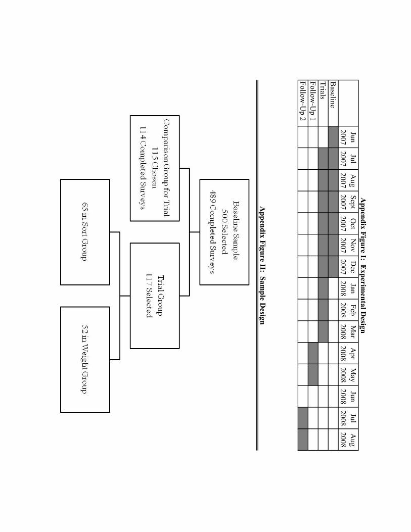
JunJul

Aug

SeptO

ctN

ovD

ecJan

FebM

arA

prM

ayJun

JulA

ug2007

20072007

20072007

20072007

20082008

20082008

20082008

20082008

Baseline

TrialsFollow

-Up 1

Follow-U

p 2

Appendix Figure I: E

xperimental D

esign

Appendix Figure II: Sam

ple Design

A. Weight Example

B. Sort Example

Appendix Figure III: Examples of Summarized Trial Results