HAL Id: hal-00114106https://hal.archives-ouvertes.fr/hal-00114106

Submitted on 15 Nov 2006

HAL is a multi-disciplinary open accessarchive for the deposit and dissemination of sci-entific research documents, whether they are pub-lished or not. The documents may come fromteaching and research institutions in France orabroad, or from public or private research centers.

L’archive ouverte pluridisciplinaire HAL, estdestinée au dépôt et à la diffusion de documentsscientifiques de niveau recherche, publiés ou non,émanant des établissements d’enseignement et derecherche français ou étrangers, des laboratoirespublics ou privés.

Learning Stochastic Edit Distance: application inhandwritten character recognition

Jose Oncina, Marc Sebban

To cite this version:Jose Oncina, Marc Sebban. Learning Stochastic Edit Distance: application in handwritten characterrecognition. Pattern Recognition, Elsevier, 2006, 39, pp.1575-1587. <hal-00114106>

Learning Stochastic Edit Distance: application inhandwritten character recognition ?

Jose Oncinaa,1 Marc Sebbanb,2

a Departamento de Lenguajes y Sistemas Informaticos, Universidad de Alicante, E-03071Alicante (Spain)

b EURISE, Universite de Saint-Etienne, 23 rue du Docteur Paul Michelon, 42023Saint-Eienne (France)

Abstract

Many pattern recognition algorithms are based on the nearest neighbour search and usethe well known edit distance, for which the primitive edit costs are usually fixed in ad-vance. In this article, we aim at learning anunbiasedstochastic edit distance in the formof a finite-state transducer from a corpus of (input,output) pairs of strings. Contrary to theother standard methods, which generally use the Expectation Maximisation algorithm, ouralgorithm learns a transducer independently on the marginal probability distribution of theinput strings. Such an unbiased way to proceed requires to optimise the parameters of aconditional transducer instead of ajoint one. We apply our new model in the context ofhandwritten digit recognition. We show, carrying out a large series of experiments, that italways outperforms the standard edit distance.

Key words: Stochastic Edit Distance, Finite-State Transducers, Handwritten characterrecognition

? This work was supported in part by the IST Programme of the European Community,under the PASCAL Network of Excellence, IST-2002-506778. This publicationonly reflectsthe authors’ views.

Email addresses:oncina@dlsi.ua.es (Jose Oncina ),marc.sebban@univ-st-etienne.fr (Marc Sebban ).1 The author thanks the Generalitat Valenciana for partial support of this work throughproject GV04B-631, this work was also supported by the Spanish CICyT trough projectTIC2003-08496-C04, partially supported by the EU ERDF.2 This work was done when the author visited the Departamento de Lenguajes y SistemasInformaticos of the University of Alicante, Spain. The visit was sponsored by the SpanishMinistry of Education trough project SAB2003-0067.

Preprint submitted to Elsevier Science 15 March 2006

1 Introduction

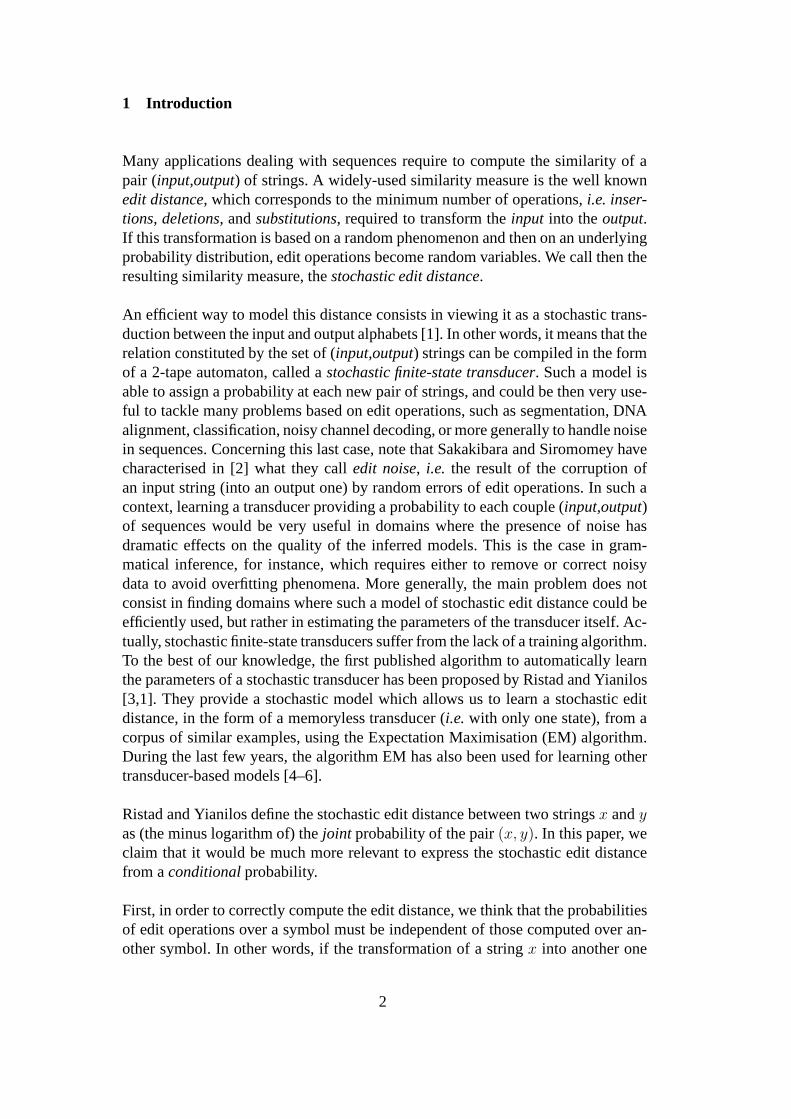
Many applications dealing with sequences require to compute the similarity of apair (input,output) of strings. A widely-used similarity measure is the well knownedit distance, which corresponds to the minimum number of operations,i.e. inser-tions, deletions, andsubstitutions, required to transform theinput into theoutput.If this transformation is based on a random phenomenon and then on an underlyingprobability distribution, edit operations become random variables. We call then theresulting similarity measure, thestochastic edit distance.

An efficient way to model this distance consists in viewing itas a stochastic trans-duction between the input and output alphabets [1]. In otherwords, it means that therelation constituted by the set of (input,output) strings can be compiled in the formof a 2-tape automaton, called astochastic finite-state transducer. Such a model isable to assign a probability at each new pair of strings, and could be then very use-ful to tackle many problems based on edit operations, such assegmentation, DNAalignment, classification, noisy channel decoding, or moregenerally to handle noisein sequences. Concerning this last case, note that Sakakibara and Siromomey havecharacterised in [2] what they calledit noise, i.e. the result of the corruption ofan input string (into an output one) by random errors of edit operations. In such acontext, learning a transducer providing a probability to each couple (input,output)of sequences would be very useful in domains where the presence of noise hasdramatic effects on the quality of the inferred models. Thisis the case in gram-matical inference, for instance, which requires either to remove or correct noisydata to avoid overfitting phenomena. More generally, the main problem does notconsist in finding domains where such a model of stochastic edit distance could beefficiently used, but rather in estimating the parameters ofthe transducer itself. Ac-tually, stochastic finite-state transducers suffer from the lack of a training algorithm.To the best of our knowledge, the first published algorithm toautomatically learnthe parameters of a stochastic transducer has been proposedby Ristad and Yianilos[3,1]. They provide a stochastic model which allows us to learn a stochastic editdistance, in the form of a memoryless transducer (i.e. with only one state), from acorpus of similar examples, using the Expectation Maximisation (EM) algorithm.During the last few years, the algorithm EM has also been usedfor learning othertransducer-based models [4–6].

Ristad and Yianilos define the stochastic edit distance between two stringsx andyas (the minus logarithm of) thejoint probability of the pair(x, y). In this paper, weclaim that it would be much more relevant to express the stochastic edit distancefrom aconditionalprobability.

First, in order to correctly compute the edit distance, we think that the probabilitiesof edit operations over a symbol must be independent of thosecomputed over an-other symbol. In other words, if the transformation of a string x into another one

2

y does not require many edit operations, it is expected that the probability of thesubstitution of a symbol by itself should be high. But, as thesum of the probabili-ties of all edit operations is one, then the probability of the substitution of anothersymbol by itself can not obviously be too large. Thus, by using a joint distribution(summing to 1), one generates an awkward dependence betweenedit operations.

Moreover, we think that the primitive edit costs of the edit distance must be in-dependent of thea priori distribution p(x) of the input strings. However,p(x)can be directly deduced from the joint distributionp(x, y), as follows:p(x) =∑

y∈Y ∗ p(x, y), whereY ∗ is the set of all finite strings over the output alphabetY . This means that this information is totally included in thejoint distribution. Bydefining the stochastic edit distance as a function of the joint probability, as donein [1], the edit costs are then dependent ofp(x). However, if we use a conditionaldistribution, this dependence is removed, since it is impossible to obtainp(x) fromp(y|x) alone.

Finally, although it is sensible and practical to model the stochastic edit distanceby a memoryless transducer, it is possible that thea priori distributionp(x) maynot be modelled by such a very simple structure. Thus, by learning a transducerdefining the joint distributionp(x, y), its parameters can converge to compromisevalues and not to the true ones. This can have dramatic effects from an applicationstandpoint. Actually, a widely-used solution to find an optimal output stringy ac-cording to an input onex consists in first learning the joint distribution transducerand later deducing the conditional transducer dividing byp(x) (more precisely byits estimates over the learning set). Such a strategy is thenirrelevant for the reasonwe mentioned above.

In this paper we have developed a way to learn directly the conditional transducer.After some definitions and notations (Section 2), we introduce in Section 3 thelearning principle of the stochastic edit distance proposed by Ristad and Yianilos[3,1]. Then, by simulating different theoretical joint distributions, we show that theunique way, using their algorithm, to find them consists in sampling a learning setof (x, y) pairs according to the marginal distribution (i.e. over the input strings)of the target joint distribution itself. Moreover, we show that for all othera prioridistribution, the difference between the target and the learned models increases.To free the method from this bias, one mustdirectly learn at each iteration of thealgorithm EM the conditional distributionp(y|x). Achieving this task requires tomodify Ristad and Yianilos’s framework. That is the goal of Section 4. Finally, inSection 5, we carry out a large series of experiments on handwritten digit recogni-tion. Through more than 1 million of tests, we show the relevance of our new modelin comparison with the standard edit distance.

3

2 Classic String Edit Distance

An alphabetX is a finite nonempty set of symbols.X∗ denotes the set of all finitestrings overX. Letx ∈ X∗ be an arbitrary string of length|x| over the alphabetX.In the following, unless stated otherwise, symbols are indicated bya, b, . . . , stringsbyu, v, . . . , z, and the empty string byε. R

+ is the set of non negative reals. Letf(·)be a function, from which[f(x)]π(x,... ) is equal tof(x) if the predicateπ(x, . . . )holds and 0 otherwise, wherex is a (set of) dummy variable(s).

A string edit distance is characterised by a triple(X, Y, ce) consisting of the finitealphabetsX and Y and the primitive cost functionce : E → R

+ whereE =Es ∪ Ed ∪ Ei is the alphabet of primitive edit operations,Es = X × Y , is the setof substitutions,Ed = X × {ε} is the set of deletions,Ei = {ε} × Y is the set ofinsertions. Each such triple(X, Y, ce) induces a distance functiond : X∗ × Y ∗ →R

+ that maps a pair of strings to a non negative real value. The edit distanced(x, y)between two stringsx ∈ X andy ∈ Y is defined recursively as:

d(x, y) = min

[ce(a, b) + d(x′, y′)]x=x′a∧y=y′b

[ce(a, ε) + d(x′, y)]x=x′a

[ce(ε, y) + dc(x, y′)]y=y′b

Note thatd(x, y) can be computed inO(|x| · |y|) time using dynamic programming.

3 Stochastic Edit Distance and Memoryless Transducers

If the edit operations are achieved according to a random process, the edit distanceis then called thestochastic edit distance, and notedds(x, y). Since the underlyingprobability distribution is unknown, one solution consists in learning the primitiveedit costs by means of a suited model. In this paper, we used memoryless transduc-ers. Transducers are currently used in many applications ranging from lexical anal-ysers, language and speech processing, etc. They are able tohandle large amountof data, in the form of pairs of (x, y) sequences, in a reasonable time complexity.Moreover, assuming that edit operations are randomly and independently achieved(that is the case in the edit noise [2]), a memoryless transducer is sufficient to modelthe stochastic edit distance.

4

3.1 Joint Memoryless Transducers

A joint memoryless transducer defines a joint probability distribution over the pairsof strings. It is denoted by a tuple(X, Y, c, γ) whereX is the input alphabet,Y isthe output alphabet,c is theprimitive joint probability function,c : E → [0, 1] andγ is the probability of the termination symbol of a string. As(ε, ε) 6∈ E, in order tosimplify the notations, we are going to usec(ε, ε) andγ as synonyms.

Let us assume for the moment that we know the probability function c (in fact,we will learn it later). We are then able to compute the joint probability p(x, y)of a pair of strings(x, y). Actually, the joint probabilityp : X∗ × Y ∗ → [0, 1]of the stringsx, y can be recursively computed by means of an auxiliary function(forward)α : X∗ × Y ∗ → R

+ as:

α(x, y) = [1]x=ε∧y=ε

+ [c(a, b) · α(x′, y′)]x=x′a∧y=y′b

+ [c(a, ε) · α(x′, y)]x=x′a

+ [c(ε, b) · α(x, y′)]y=y′b.

And then,

p(x, y) = α(x, y)γ.

In a symmetric way,p(x, y) can be recursively computed by means of an auxiliaryfunction (backward)β : X∗ × Y ∗ → R

+ as:

β(x, y) = [1]x=ε∧y=ε

+ [c(a, b) · β(x′, y′)]x=ax′∧y=by′

+ [c(a, ε) · β(x′, y)]x=ax′

+ [c(ε, b) · β(x, y′)]y=by′ .

And then,

p(x, y) = β(x, y)γ.

Both functions (forward and backward) can be computed inO(|x| · |y|) time usinga dynamic programming technique. This model defines a probability distributionover the pairs (x, y) of strings. More precisely,

∑

x∈X∗

∑

y∈Y ∗

p(x, y) = 1,

5

that is achieved if the following conditions are fulfilled [1],

γ > 0, c(a, b), c(ε, b), c(a, ε) ≥ 0 ∀a ∈ X, b ∈ Y∑

a∈X∪{ε}b∈Y ∪{ε}

c(a, b) = 1

Givenp(x, y), we can then compute, as mentioned in [1], the stochastic edit dis-tance betweenx andy. Actually, the stochastic edit distanceds(x, y) is defined asbeing the negative logarithm of the probability of the string pairp(x, y) accordingto the memoryless stochastic transducer.

ds(x, y) = − log p(x, y), ∀x ∈ X∗, ∀y ∈ Y ∗

In order to computeds(x, y), a remaining step consists in learning the parametersc(a, b) of the memoryless transducer,i.e. the primitive edit costs.

3.2 Optimisation of the parameters of the joint memoryless transducer

Let S be a finite set of (x, y) pairs ofsimilar strings. Ristad and Yianilos [1] pro-pose to use the expectation-maximisation (EM) algorithm tofind the optimal jointstochastic transducer. The EM algorithm consists in two steps (expectation andmaximisation) that are repeated until a convergence criterion is achieved.

Given an auxiliary(|X| + 1) × (|Y | + 1) matrix δ, the expectation step can bedescribed as follows:∀a ∈ X, b ∈ Y ,

δ(a, b) =∑

(xax′,yby′)∈S

α(x, y)c(a, b)β(x′, y′)γ

p(xax′, yby′)

δ(ε, b) =∑

(xx′,yby′)∈S

α(x, y)c(ε, b)β(x′, y′)γ

p(xx′, yby′)

δ(a, ε) =∑

(xax′,yy′)∈S

α(x, y)c(a, ε)β(x′, y′)γ

p(xax′, yy′)

δ(ε, ε) =∑

(x,y)∈S

α(x, y)γ

p(x, y)= |S|,

and the maximisation:

c(a, b) =δ(a, b)

N∀a ∈ X ∪ {ε}, ∀b ∈ Y ∪ {ε}

6

c∗(a, b) ε a b c d c∗(a)

ε 0.00 0.05 0.08 0.02 0.02 0.17

a 0.01 0.04 0.01 0.01 0.01 0.08

b 0.02 0.01 0.16 0.04 0.01 0.24

c 0.01 0.02 0.01 0.15 0.00 0.19

d 0.01 0.01 0.01 0.01 0.28 0.32Table 1Target joint distributionc∗(a, b) and its corresponding marginal distributionc∗(a).

where

N =∑

a∈X∪{ε}b∈Y ∪{ε}

δ(a, b).

3.3 Limits of Ristad and Yianilos’s algorithm

To analyse the ability of Ristad and Yianilos’s algorithm tocorrectly estimate theparameters of a target joint memoryless transducer, we haveimplemented it andcarried out a series of experiments. Since the joint distributionp(x, y) is a functionof the learned edit costsc(a, b), we only focused here on the functionc of thetransducer.

The experimental setup was the following. We simulated a target joint memory-less transducer from the alphabetsX = Y = {a, b, c, d}, such as∀a ∈ X ∪{ε}, ∀b ∈ Y ∪ {ε}, the target model is able to return the primitive theoreticaljoint probabilityc∗(a, b). The target joint distribution we used is described in Ta-ble 13 . The marginal distributionc∗(a) can be deduced from this target such that:c∗(a) =

∑

b∈X∪{ε} c∗(a, b).

Then, we sampled an increasing set of learning input strings(from 0 to 4000 se-quences) of variable length generated from a given probability distribution p(a)over the input alphabetX. In order to simplify, we modelled this distribution inthe form of an automaton with only one state4 and |X| output transitions withrandomly chosen probabilities satisfying that

∑

a∈X p(a) + p(#) = 1, wherep(#)corresponds to the probability of a termination symbol of a string (see Figure 1).

3 Note that we carried out many series of experiments with various target joint distribu-tions, and all the results we obtained follow the same behaviour as the one presented in thissection.4 Here also, we tested other configurations leading to the sameresults.

7

p(#)

a: p(a)b: p(b)c: p(c)d: p(d)

Fig. 1. Automaton used for generating the input sequences. The probabilityp(#) corre-sponds to the probability of a termination symbol of a string, or in other words the proba-bility of the state to be final.

We used different settings for this automaton to analyse theimpact of the inputdistributionp(a) on the learned joint model. Then, given an input sequencex (gen-erated from this automaton) and the target joint distribution c∗(a, b), we sampleda corresponding outputy. Finally, the setS of generated (x, y) pairs was used byRistad and Yianilos’s algorithm to learn an estimated primitive joint distributionc(a, b).

We compared the target and the learned distributions to analyse the behaviour ofthe algorithm to correctly assess the parameters of the target joint distribution. Wecomputed an average difference between the both, defined as follows:

d(c, c∗) =

∑

a∈X∪{ε}

∑

b∈Y ∪{ε} |c(a, b) − c∗(a, b)|

2

Normalised in this way,d(c, c∗) is a value in the range[0, 1]. Figure 2 shows thebehaviour of this difference according to various configurations of the automatonof Figure 1. We can note that the unique way to converge towards a difference nearfrom 0 consists in using the marginal distributionc∗(a) of the target for generatingthe input strings. For all the other ways, the difference becomes very large.

As we said at the beginning of this article, we can easily explain this behaviour. Bylearning the primitive joint probability functionc(a, b), Ristad and Yianilos learnat the same time the marginal distributionc(a). The learned edit costs (and thestochastic edit distance) are then dependent of thea priori distribution of the in-put strings, that is obviously awkward. To free of this statistical bias, we have tolearn the primitive conditional probability function independently of the marginaldistribution. That is the goal of the next section.

8

0

0.05

0.1

0.15

0.2

0.25

0.3

0.35

0.4

0.45

500 1000 1500 2000 2500 3000 3500 4000

Dis

tanc

e be

twee

n th

eore

tical

and

lear

nt tr

ansd

ucer

s

Number of Strings

a (0.08) b (0.24) c (0.19) d (0.32) # (0.17) a (0.06) b (0.28) c (0.03) d (0.32) # (0.31) a (0.07) b (0.28) c (0.01) d (0.40) # (0.24) a (0.12) b (0.15) c (0.26) d (0.14) # (0.32) a (0.28) b (0.23) c (0.15) d (0.02) # (0.32)

Fig. 2. Average difference between the target and the learned distributions according tovarious generations of the input strings.

4 Unbiased Learning of a Conditional Memoryless Transducer

A conditional memoryless transducer is denoted by a tuple(X, Y, c, γ) whereX isthe input alphabet,Y is the output alphabet,c is the primitive conditional probabil-ity function c : E → [0, 1] andγ is the probability of the termination symbol of astring. As in the joint case, since(ε, ε) 6∈ E, in order to simplify the notation weuseγ andc(ε|ε) as synonyms.

The probabilityp : X∗ × Y ∗ → [0, 1] of the stringy assuming the input one wasa x (notedp(y|x)) can be recursively computed by means of an auxiliary function(forward)α : X∗ × Y ∗ → R

+ as:

α(y|x) = [1]x=ε∧y=ε

+ [c(b|a) · α(y′|x′)]x=x′a∧y=y′b

+ [c(ε|a) · α(y|x′)]x=x′a

+ [c(b|ε) · α(y′|x)]y=y′b.

And then,

p(y|x) = α(y|x)γ.

In a symmetric way,p(y|x) can be recursively computed by means of an auxiliary

9

function (backward)β : X∗ × Y ∗ → R+ as:

β(y|x) = [1]x=ε∧y=ε

+ [c(b|a) · β(y′|x′)]x=ax′∧y=by′

+ [c(ε|a) · β(y|x′)]x=ax′

+ [c(b|ε) · β(y′|x)]y=by′ .

And then,

p(y|x) = β(y|x)γ.

As in the joint case, both functions can be computed inO(|x| · |y|) time using a dy-namic programming technique. In this model a probability distribution is assignedconditionally to each input string. Then

∑

y∈Y ∗

p(y|x) ∈ {1, 0} ∀x ∈ X∗.

The0 is in the case the input stringx is not in the domain of the function5 . It canbe show (see Annex) that the normalisation of each conditional distribution can beachieved if the following conditions over the functionc and the parameterγ arefulfilled,

γ > 0, c(b|a), c(b|ε), c(ε|a) ≥ 0 ∀a ∈ X, b ∈ Y (1)∑

b∈Y

c(b|ε) +∑

b∈Y

c(b|a) + c(ε|a) = 1 ∀a ∈ X (2)

∑

b∈Y

c(b|ε) + γ = 1 (3)

As in the joint case, the expectation-maximisation algorithm can be used in orderthe find the optimal parameters. The expectation step deals with the computationof the matrixδ:

δ(b|a) =∑

(xax′,yby′)∈S

α(y|x)c(b|a)β(y′|x′)γ

p(yby′|xax′)

δ(b|ε) =∑

(xx′,yby′)∈S

α(y|x)c(b|ε)β(y′|x′)γ

p(yby′|xx′)

δ(ε|a) =∑

(xax′,yy′)∈S

α(y|x)c(ε|a)β(y′|x′)γ

p(yy′|xax′)

δ(ε|ε) =∑

(x,y)∈S

α(y|x)γ

p(y|x)= |S|.

5 If p(x) = 0 thenp(x, y) = 0 and asp(y|x) = p(x,y)p(x) we have a0

0 indeterminism. We

chose to solve it taking00 = 0, in order to maintain∑

y∈Y ∗ p(y|x) finite.

10

The maximisation step allows us to deduce the current edit costs.

c(b|ε) =δ(b|ε)

Nγ =

N − N(ε)

N

c(b|a) =δ(b|a)

N(a)

N − N(ε)

Nc(ε|a) =

δ(ε|a)

N(a)

N − N(ε)

N

where:

N =∑

a∈X∪{ε}b∈Y ∪{ε}

δ(b|a) N(ε) =∑

b∈Y

δ(b|ε) N(a) =∑

b∈Y ∪{ε}

δ(b|a)

For further details about these two stages see Annex 2.

We carried out experiments to assess the relevance of our newlearning algorithmto correctly estimate the parameters of target transducers. We followed exactly thesame experimental setup as the one of Section 3.3, except to the definition of ourdifferenced(c, c∗). Actually, as we said before, our new framework estimates|X|conditional distributions. Sod(c, c∗) is defined as follows :

d(c, c∗) =(A + B |X|)

2 |X|

where

A =∑

a∈X

∑

b∈Y ∪{ε}

|c(b|a) − c∗(b|a)|

and

B =∑

b∈Y ∪{ε}

|c(b|ε) − c∗(b|ε)|

The results are shown in Figure 3. We can make the two following remarks. First,the different curves clearly show that the convergence toward the target distributionis independent of the distribution of the input strings. Using different parameterconfigurations of the automaton of Figure 1, the behaviour ofour algorithm re-mains the same,i.e the difference between the learned and the target conditionaldistributions tends to 0. Second, we can note thatd(c, c∗) rapidly decreases,i.e. thealgorithm requires few learning examples to learn the target.

11

0

0.02

0.04

0.06

0.08

0.1

0.12

0.14

0.16

0.18

500 1000 1500 2000 2500 3000 3500 4000

Dis

tanc

e be

twee

n th

eore

tical

and

lear

nt tr

ansd

ucer

s

Number of Strings

a (0.10) b (0.17) c (0.26) d (0.20) # (0.28) a (0.09) b (0.29) c (0.04) d (0.27) # (0.31) a (0.15) b (0.18) c (0.32) d (0.15) # (0.20) a (0.23) b (0.32) c (0.13) d (0.05) # (0.27) a (0.18) b (0.23) c (0.16) d (0.15) # (0.28)

Fig. 3. Average difference between the target and the learned conditional distributions ac-cording to various generations of the input strings.

start

Primitives

2

34

5

6

70 1

"2"=2222224324444466656565432222222466666666660000212121210076666546600210

Fig. 4. Example of string coding character.

5 Application to the handwritten character recognition

5.1 Description of the database - Constitution of the set of pairs

In order to assess the relevance of our model in a pattern recognition task, weapplied it on the real world problem of handwritten digit classification. We used

12

the NIST Special Database 3 of the National Institute of Standards and Technology,already used in several articles such as [7–9]. This database consists in 128× 128bitmap images of handwritten digits and letters. In this series of experiments, weonly focus on digits written by 100 different writers. Each class of digit (from 0to 9) has about 1,000 instances, then the whole database we used contains about10,000 handwritten digits. As we will explain later, a part of them will be used asa learning setLS, the remaining digits being kept in a test sampleTS. Since ourmodel handles strings, we coded each digit as an octal string, following the featureextraction algorithm proposed in [7]. It consists in scanning the bitmap left-to-rightand starting from the top. When the first pixel is found, it follows the border of thecharacter until it returns to the first pixel. During this traversal, the algorithm buildsa string with the absolute direction of the next pixel in the border. Fig. 4 describesan example on a given “2”. The vector of features in the form ofa octal string ispresented at the bottom of the figure.

As presenting throughout this article, our method requiresa set of (input,output)pairs of strings for learning the probabilistic transducer. As we claimed before, thededuced stochastic edit distance can then be efficiently used for classification, se-quence alignment, or noise correction. While it is rather clear in this last case thatpairs in the form of (noisy,unnoisy) strings constitute themost relevant way to learnan edit distance useful in a noise correction model, what must they represent in apattern recognition task, with various classes, such as in handwritten digit classi-fication? As already proposed in [1], a possible solution consists in building pairsof “similar” strings that describe the possible variationsor distortions between in-stances of each class. Such pairs can be drawn by an expert of the area. In thisseries of experiments on handwritten digits, we decided rather to automaticallybuild pairs of (input,output) strings, where an input is a learning string ofLS, andthe output is a prototype of the input. We used as prototype the corresponding 1-nearest-neighbour inLS of each input. On the one hand, this choice is motivatedfrom an algorithmic standpoint. Actually, with a learning set constituted of|LS|examples, such a strategy does not increase the complexity of the algorithm using|LS| pairs of strings too. On the other hand, by attributing the nearest digit to eachcharacter, we ensure to model the main possible distortionsbetween digits in eachclass.

Note that we could have used other ways to construct string pairs. A solution wouldbe to generate all pairs in the same class. Beyond large complexity costs, this strat-egy would not be relevant in such a digit recognition task. Actually, the classes ofdigits are intrinsically multimodal. For example a zero canbe written either with anopen loop or a closed one. In this case, the string that represents an “open” zero cannot be considered as a distortion of a “closed” zero, but rather as a different manner(a sort of sub-class) to design this digit. That explains that a nearest-neighbor basedstrategy is much more relevant.

To achieve this task, we used here a classic edit distance forcomputing the nearest-

13

neighbour,i.e. with the same edit cost for an insertion, deletion or a substitution.The objective is then to learn a stochastic transducer that allows to optimise theconditional probabilitiesp(output/input).

5.2 Experimental setup

We claim that learning the primitive edit costs of an edit distance in the form ofa conditional transducer is more relevant not only than learning a joint transducer,but also than fixing these costs in advance by an expert. Therefore, in the followingseries of experiments, we aim at comparing our approach (i) to the one of Ristad andYianilos, and (ii) to the classic edit distance. The experimental setup, graphicallydescribed in Fig. 5, is the following:

(1) Learning Stage• Step 1: each seti of digits (i = 0, .., 9) is divided in two parts: a learning set

LSi and a test setTSi.• Step 2: from eachLSi, we build a set of string pairsPSi in the form(x, NN(x)),∀x ∈ LSi, whereNN(x) = argminy∈LSi−{x}dE(x, y) (dE is the classicedit distance).

• Step 3: we learn a uniqueconditionaltransducer from∪iPSi.• Step 4: we learn a uniquejoint transducer from∪iPSi.

(2) Test Stage• Step 5: we classify each test digitx′ ∈ ∪iTSi,

· by the classi of the learning stringy ∈ ∪iLSi maximisingp(y|x′)(using the conditional transducer)

· by the classi of the learning stringy ∈ ∪iLSi maximisingp(x′, y)(using the joint transducer)

· by the classi of its nearest-neighbourNN(x′) ∈ ∪iLSi

Using the previous experimental setup, we can then compare the three approachesunder exactly the same conditions. Actually, during the test stage, each algorithmuses:

• one matrix concerning the primitive edit operations (ana priori fixed matrix ofedit costsfor the nearest-neighbour algorithm, a learned matrix ofedit probabil-ities for the two others),

• the union of the learning setsLSi.• the classic edit distance algorithm (for the nearest-neighbour algorithm), or its

probabilistic version (for the others).

Note that for the standard edit distance, we used two different matrices of edit costs.The first one is the most classic one,i.e. each edit operation has the same cost(here, 1). According to [8], a more relevant strategy would consist in taking costsproportionally to the relative angle between the directions used for describing a

14

Class 0

Class 1

Class 9

.

.

.

.

.

.

TS0

LS

LS1

TS9

LS9

01

X’0N’

X’

...

X

X0N

X’11

...

X’1N’

X11

...

X1N

X’

X’9N’

91X

...

X9N

91

01

...

...

01

0N

PS0

0

0N

PS

11 11

1N 1N

...

...

PS

1

9

91 91

9N 9N

.

.

. .

.

.

STEP 1 STEP 2

STEP 3

Conditional Transducer

Learning

STEP 4

STEP 5

a conditional transducer

Accuracy using

a joint transducer

Accuracy using

the Nearest−Neighbor

Accuracy using

(X , NN( X ))01

(X , NN( X ))

(X , NN( X ))

(X , NN( X ))

(X , NN( X ))

(X , NN( X ))

1TS

Joint Transducer

Learning

Algorithm

Nearest−Neighbor

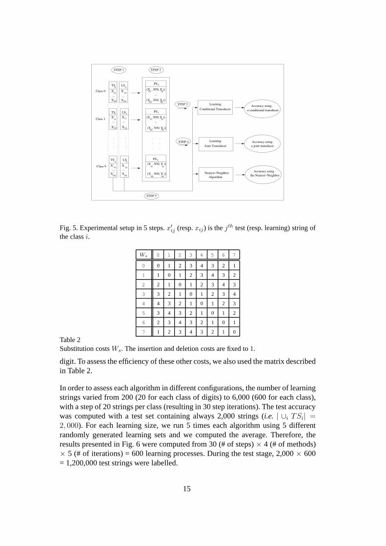
Fig. 5. Experimental setup in 5 steps.x′ij (resp.xij) is thejth test (resp. learning) string of

the classi.

Ws 0 1 2 3 4 5 6 7

0 0 1 2 3 4 3 2 1

1 1 0 1 2 3 4 3 2

2 2 1 0 1 2 3 4 3

3 3 2 1 0 1 2 3 4

4 4 3 2 1 0 1 2 3

5 3 4 3 2 1 0 1 2

6 2 3 4 3 2 1 0 1

7 1 2 3 4 3 2 1 0

Table 2Substitution costsWs. The insertion and deletion costs are fixed to1.

digit. To assess the efficiency of these other costs, we also used the matrix describedin Table 2.

In order to assess each algorithm in different configurations, the number of learningstrings varied from 200 (20 for each class of digits) to 6,000(600 for each class),with a step of 20 strings per class (resulting in 30 step iterations). The test accuracywas computed with a test set containing always 2,000 strings(i.e. | ∪i TSi| =2, 000). For each learning size, we run 5 times each algorithm using5 differentrandomly generated learning sets and we computed the average. Therefore, theresults presented in Fig. 6 were computed from 30 (# of steps)× 4 (# of methods)× 5 (# of iterations) = 600 learning processes. During the teststage, 2,000× 600= 1,200,000 test strings were labelled.

15

82

84

86

88

90

92

94

96

98

100

0 1000 2000 3000 4000 5000 6000

Tes

t Acc

urac

y

Number of Learning Pairs

Learned ED with a Conditional TransducerClassic ED (using costs of Table 2)

Classic ED (using costs 111)Learned ED with a Joint Transducer

Fig. 6. Test accuracy on the handwritten digits.

5.3 Results and Discussion

From Fig. 6, we can make the following remarks.

First of all, learning an edit distance in the form of a conditional transducer is in-disputably relevant to achieve a pattern recognition task.Whatever the size of thelearning set, the test accuracy obtained using the stochastic edit distance is higherthan the others. However, note that the difference decreases logically with the sizeof the learning set. Actually, from a theoretical standpoint, lim|LS|→∞P (d(x, NN(x)) >ε) = 0, ∀ε > 0. In other words, it means that whatever the distance we choose,when the number of examples increases, the nearest-neighbour of an examplextends to bex itself. Interestingly, we can also note that for reaching approximatelythe same accuracy rate, the standard edit distance (using costs of Table 2) needsmuch more learning strings, and therefore requires a highertime complexity, thanour approach.

Second, the results obtained with Ristad and Yianilos’s method are logical andeasily interpretable. When the number of learning string pair is small, all the draw-backs we already mentioned in the first part of this paper occur. Actually, whilea nearest-neighbour is always a string belonging to the learning set, many learn-ing strings are not present in the current (small) set of nearest-neighbours. There-

16

0

0.1

0.2

0.3

0.4

0.5

0.6

0.7

0.8

0.9

0 1000 2000 3000 4000 5000 6000

Var

ianc

e

Number of Learning Pairs

Learned ED with a Conditional TransducerClassic ED (using costs of Table 2)

Fig. 7. Evolution of the variance throughout the iterations.

fore, while all these strings (inputs and outputs) come fromthe same set of digits(∪iLSi), the distribution over the outputs (the nearest-neighbours) is not the sameas the distribution over the inputs (the learning strings).Of course, this bias de-creases with the rise of the learning set size, but not sufficiently in this series ofexperiments for improving the performances of the classic edit distance.

Moreover, as already noted in [8], the use of the matrix of costs of Table 2 providesbetter results than the naıve configuration consisting in using the same cost forthe three edit operations. Even if the difference is not important between the twocurves, the first one is always higher than the second. However, it is not sufficientto beat the learned edit distance with a conditional transducer. To assess the levelof stability of the approaches, we have computed a measure ofdispersion on theresults provided by the standard edit distance (with costs of Table 2) and our learneddistance. Fig. 7 shows the behaviour of the variance of the test accuracy throughoutthe iterations. Interestingly, we can note that in the largemajority of the cases, ourmethod gives a smaller variance.

17

6 Conclusion

In this paper, we proposed a relevant approach for learning the stochastic edit dis-tance in the form of a memoryless transducer. While the standard techniques aim atlearning a joint distribution over the edit operations, we showed that such a strategyinduces a bias in the form of a statistical dependence on the input string distribu-tion. We overcame this drawback by directly learning a conditional distribution ofthe primitive edit costs. The experimental results on a handwritten digit recognitiontask bring to the fore the interest of our approach.

We think that this work deserves further investigations. First, we believe that theway to build the pairs of strings can be efficiently improved.So far, we used as pro-totype, the nearest-neighbour of each learning string. Thek-nearest-neighbours, orclustering-based strategies should be studied in our future works. We have also tostudy an adaptive strategy which would update the learning set of pairs by using ateach iteration of the EM algorithm the edit costs learned during the previous stage.Second, beyond its good behaviour for dealing with a classification task, our modelcan be also particularly suited for handling noisy data. Actually, it can be used tocorrect noisy learning instances before any inference process. Moreover, we alsoplan to extend our work on semi-structured data, such as trees. One of our ob-jective consists in improving classification performancesfor applications in musicretrieval, which handles tree-based representations for identifying new melodies.

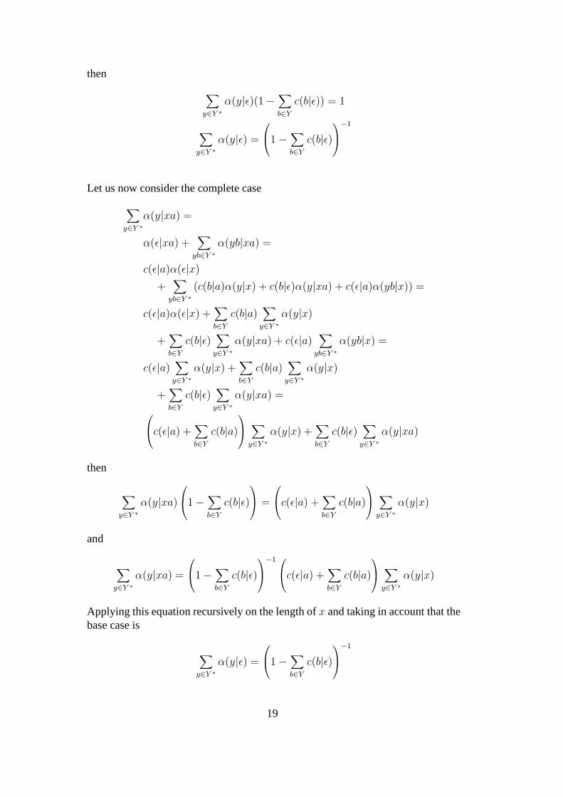
Annex 1

We are going to show that eq. 1, 2 and 3 are sufficient to satisfy

∑

y∈Y ∗

p(y|x) = 1.

Let us first consider the case whenx = ε.

∑

y∈Y ∗

α(y|ε) = 1 +∑

yb∈Y ∗

α(yb|ε)

= 1 +∑

yb∈Y ∗

c(b|ε)α(y|ε)

= 1 +∑

b∈Y

c(b|ε)∑

y∈Y ∗

α(y|ε)

18

then

∑

y∈Y ∗

α(y|ε)(1−∑

b∈Y

c(b|ε)) = 1

∑

y∈Y ∗

α(y|ε) =

1 −∑

b∈Y

c(b|ε)

−1

Let us now consider the complete case

∑

y∈Y ∗

α(y|xa) =

α(ε|xa) +∑

yb∈Y ∗

α(yb|xa) =

c(ε|a)α(ε|x)

+∑

yb∈Y ∗

(c(b|a)α(y|x) + c(b|ε)α(y|xa) + c(ε|a)α(yb|x)) =

c(ε|a)α(ε|x) +∑

b∈Y

c(b|a)∑

y∈Y ∗

α(y|x)

+∑

b∈Y

c(b|ε)∑

y∈Y ∗

α(y|xa) + c(ε|a)∑

yb∈Y ∗

α(yb|x) =

c(ε|a)∑

y∈Y ∗

α(y|x) +∑

b∈Y

c(b|a)∑

y∈Y ∗

α(y|x)

+∑

b∈Y

c(b|ε)∑

y∈Y ∗

α(y|xa) =

c(ε|a) +∑

b∈Y

c(b|a)

∑

y∈Y ∗

α(y|x) +∑

b∈Y

c(b|ε)∑

y∈Y ∗

α(y|xa)

then

∑

y∈Y ∗

α(y|xa)

1 −∑

b∈Y

c(b|ε)

=

c(ε|a) +∑

b∈Y

c(b|a)

∑

y∈Y ∗

α(y|x)

and

∑

y∈Y ∗

α(y|xa) =

1 −∑

b∈Y

c(b|ε)

−1

c(ε|a) +∑

b∈Y

c(b|a)

∑

y∈Y ∗

α(y|x)

Applying this equation recursively on the length ofx and taking in account that thebase case is

∑

y∈Y ∗

α(y|ε) =

1 −∑

b∈Y

c(b|ε)

−1

19

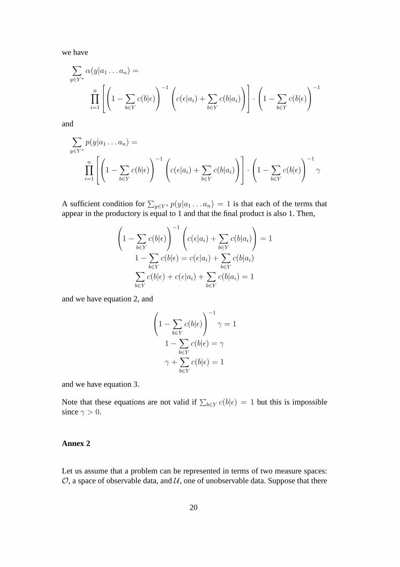
we have

∑

y∈Y ∗

α(y|a1 . . . an) =

n∏

i=1

1 −∑

b∈Y

c(b|ε)

−1

c(ε|ai) +∑

b∈Y

c(b|ai)

·

1 −∑

b∈Y

c(b|ε)

−1

and

∑

y∈Y ∗

p(y|a1 . . . an) =

n∏

i=1

1 −∑

b∈Y

c(b|ε)

−1

c(ε|ai) +∑

b∈Y

c(b|ai)

·

1 −∑

b∈Y

c(b|ε)

−1

γ

A sufficient condition for∑

y∈Y ∗ p(y|a1 . . . an) = 1 is that each of the terms thatappear in the productory is equal to 1 and that the final product is also 1. Then,

1 −∑

b∈Y

c(b|ε)

−1

c(ε|ai) +∑

b∈Y

c(b|ai)

= 1

1 −∑

b∈Y

c(b|ε) = c(ε|ai) +∑

b∈Y

c(b|ai)

∑

b∈Y

c(b|ε) + c(ε|ai) +∑

b∈Y

c(b|ai) = 1

and we have equation 2, and

1 −∑

b∈Y

c(b|ε)

−1

γ = 1

1 −∑

b∈Y

c(b|ε) = γ

γ +∑

b∈Y

c(b|ε) = 1

and we have equation 3.

Note that these equations are not valid if∑

b∈Y c(b|ε) = 1 but this is impossiblesinceγ > 0.

Annex 2

Let us assume that a problem can be represented in terms of twomeasure spaces:O, a space of observable data, andU , one of unobservable data. Suppose that there

20

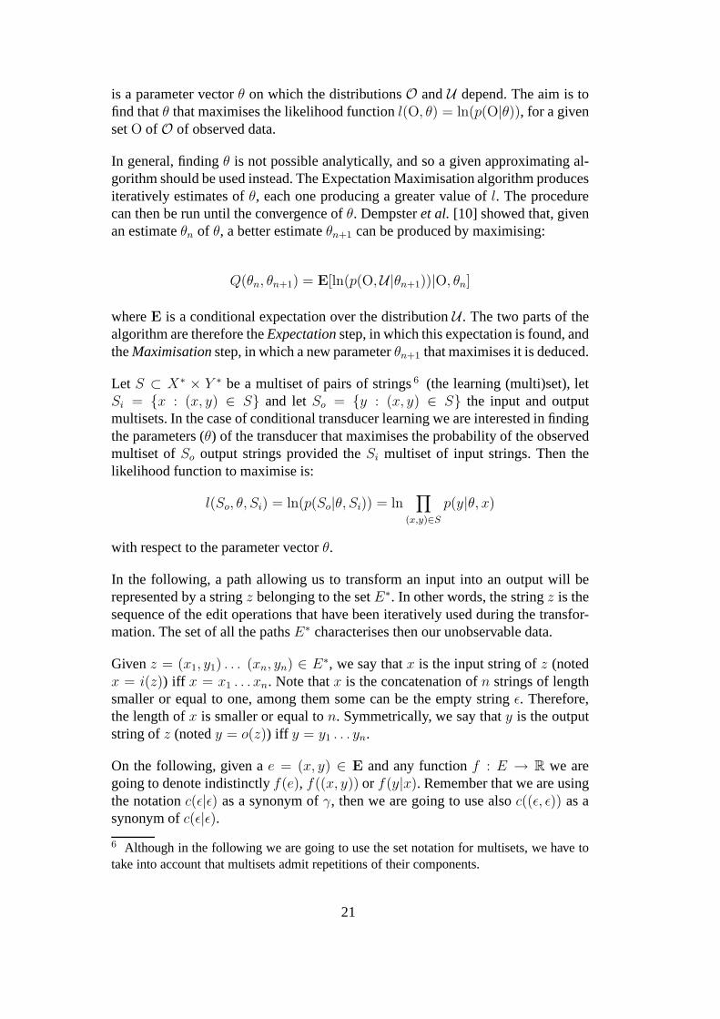
is a parameter vectorθ on which the distributionsO andU depend. The aim is tofind thatθ that maximises the likelihood functionl(O, θ) = ln(p(O|θ)), for a givensetO of O of observed data.

In general, findingθ is not possible analytically, and so a given approximating al-gorithm should be used instead. The Expectation Maximisation algorithm producesiteratively estimates ofθ, each one producing a greater value ofl. The procedurecan then be run until the convergence ofθ. Dempsteret al. [10] showed that, givenan estimateθn of θ, a better estimateθn+1 can be produced by maximising:

Q(θn, θn+1) = E[ln(p(O,U|θn+1))|O, θn]

whereE is a conditional expectation over the distributionU . The two parts of thealgorithm are therefore theExpectationstep, in which this expectation is found, andtheMaximisationstep, in which a new parameterθn+1 that maximises it is deduced.

Let S ⊂ X∗ × Y ∗ be a multiset of pairs of strings6 (the learning (multi)set), letSi = {x : (x, y) ∈ S} and letSo = {y : (x, y) ∈ S} the input and outputmultisets. In the case of conditional transducer learning we are interested in findingthe parameters (θ) of the transducer that maximises the probability of the observedmultiset ofSo output strings provided theSi multiset of input strings. Then thelikelihood function to maximise is:

l(So, θ, Si) = ln(p(So|θ, Si)) = ln∏

(x,y)∈S

p(y|θ, x)

with respect to the parameter vectorθ.

In the following, a path allowing us to transform an input into an output will berepresented by a stringz belonging to the setE∗. In other words, the stringz is thesequence of the edit operations that have been iteratively used during the transfor-mation. The set of all the pathsE∗ characterises then our unobservable data.

Givenz = (x1, y1) . . . (xn, yn) ∈ E∗, we say thatx is the input string ofz (notedx = i(z)) iff x = x1 . . . xn. Note thatx is the concatenation ofn strings of lengthsmaller or equal to one, among them some can be the empty string ε. Therefore,the length ofx is smaller or equal ton. Symmetrically, we say thaty is the outputstring ofz (notedy = o(z)) iff y = y1 . . . yn.

On the following, given ae = (x, y) ∈ E and any functionf : E → R we aregoing to denote indistinctlyf(e), f((x, y)) or f(y|x). Remember that we are usingthe notationc(ε|ε) as a synonym ofγ, then we are going to use alsoc((ε, ε)) as asynonym ofc(ε|ε).

6 Although in the following we are going to use the set notationfor multisets, we have totake into account that multisets admit repetitions of theircomponents.

21

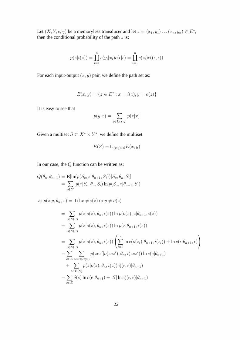
Let (X, Y, c, γ) be a memoryless transducer and letz = (x1, y1) . . . (xn, yn) ∈ E∗,then the conditional probability of the pathz is:

p(z|i(z)) =n

∏

i=1

c(yi|xi)c(ε|ε) =n

∏

i=1

c(zi)c((ε, ε))

For each input-output(x, y) pair, we define the path set as:

E(x, y) = {z ∈ E∗ : x = i(z), y = o(z)}

It is easy to see that

p(y|x) =∑

z∈E(x,y)

p(z|x)

Given a multisetS ⊂ X∗ × Y ∗, we define the multiset

E(S) = ∪(x,y)∈SE(x, y)

In our case, theQ function can be written as:

Q(θn, θn+1) = E[ln(p(So, z|θn+1, Si))|So, θn, Si]

=∑

z∈E∗

p(z|So, θn, Si) ln p(So, z|θn+1, Si)

asp(z|y, θn, x) = 0 if x 6= i(z) or y 6= o(z)

=∑

z∈E(S)

p(z|o(z), θn, i(z)) ln p(o(z), z|θn+1, i(z))

=∑

z∈E(S)

p(z|o(z), θn, i(z)) ln p(z|θn+1, i(z))

=∑

z∈E(S)

p(z|o(z), θn, i(z))

|z|∑

i=0

ln c(o(zi)|θn+1, i(zi)) + ln c(ε|θn+1, ε)

=∑

e∈E

∑

zez′∈E(S)

p(zez′|o(zez′), θn, i(zez′)) ln c(e|θn+1)

+∑

z∈E(S)

p(z|o(z), θn, i(z))c((ε, ε)|θn+1)

=∑

e∈E

δ(c) ln c(e|θn+1) + |S| ln c((ε, ε)|θn+1)

22

where

δ(e) =∑

zez′∈E(S)

p(zez′|o(zez′), θn, i(zez′))

=∑

zez′∈E(S)

p(o(zez′), zez′|θn, i(zez′))

p(o(zez′)|θn, i(zez′))

=∑

zez′∈E(S)

p(zez′|θn, i(zez′))

p(o(zez′)|θn, i(zez′))

Giving

δ(b|a) =∑

(xax′,yby′)∈S

α(y|x)c(b|a)β(y′|x′)γ

p(yby′|xax′)

δ(b|ε) =∑

(xx′,yby′)∈S

α(y|x)c(b|ε)β(y′|x′)γ

p(yby′|xx′)

δ(ε|a) =∑

(xax′,yy′)∈S

α(y|x)c(ε|a)β(y′|x′)γ

p(yy′|xax′)

as required.

Now we have to chooseθn+1 that minimises theQ(θn, θn+1) function with therestrictions:

∑

b∈Y

c((a, b)|θn+1) +∑

b∈Y

c((ε, b)|θn+1) + c((a, ε)|θn+1) = 1, ∀a ∈ X

∑

b∈Y

c((ε, b)| θn+1) + c((ε, ε)|θn+1) = 1

Using the Lagrange multipliers

L =∑

e∈E

δ(e) ln c(e|θn+1) + |S| ln c((ε, ε)|θn+1)

−∑

a∈X

µa

∑

b∈Y

c((a, b)|θn+1) +∑

b∈Y

c((ε, b)|θn+1) + c((a, ε)|θn+1) − 1

− µ

∑

b∈Y

c((ε, b)|θn+1) + c((ε, ε)|θn+1) − 1

23

Computing the derivatives and equating to zero we have:

c((a, b)|θn+1) =δ((a, b))

µa

c((ε, b)|θn+1) =δ((ε, b))

∑

a µa + µ

c((a, ε)|θn+1) =δ((a, ε))

µa

c((ε, ε)|θn+1) =|S|

µ

Substituting in the normalisation equation we obtain:

∑

b δ((ε, b))∑

a µa + µ+

∑

b δ((a, b))

µa

+δ((a, ε))

µa

= 1, ∀a ∈ X∑

b δ((ε, b))∑

a µa + µ+

|S|

µ= 1

Now we have a system with|X|+ 1 equations and|X|+ 1 unknowns. It is easy tosee that

µ = |S|N

N − N(ε)µa = N(a)

N

N − N(ε)

with

N =∑

e∈E

δ(e) + |S| N(ε) =∑

b∈Y

δ((ε, b)) N(a) =∑

b∈Y ∪{ε}

δ((a, b))

is a solution to the system.

References

[1] E. S. Ristad, P. N. Yianilos, Learning string-edit distance, IEEE Trans. Pattern Anal.Mach. Intell. 20 (5) (1998) 522–532.

[2] Y. Sakakibara, R. Siromoney, A noise model on learning sets of strings, in: COLT ’92:Proceedings of the fifth annual workshop on Computational learning theory, 1992, pp.295–302.

[3] E. S. Ristad, P. N. Yianilos, Finite growth models, Tech.Rep. CS-TR-533-96,Princeton University Computer Science Department (1996).

[4] F. Casacuberta, Probabilistic estimation of stochastic regular syntax-directedtranslation schemes, in: Proceedings of th VIth Spanish Symposium on PatternRecognition and Image Analysis, 1995, pp. 201–207.

24

[5] A. Clark, Memory-based learning of morphology with stochastic transducers, in:Proceedings of the Annual meeting of the association for computational linguistic,2002.

[6] J. Eisner, Parameter estimation for probabilistic finite-state transducers, in:Proceedings of the Annual meeting of the association for computational linguistic,2002, pp. 1–8.

[7] E. Gomez, L. Mico, J. Oncina, Testing the linear approximating eliminating searchalgorithm in handwritten character recognition tasks, in:VI Symposium Nacional dereconocimiento de Formas y Analisis de Imagenes, 1995, pp. 212–217.

[8] L. Mico, J. Oncina, Comparison of fast nearest neighbour classifiers for handwrittencharacter recognition, Pattern Recognition Letters 19 (1998) 351–356.

[9] J. R. Rico-Juan, L. Mico, Comparison of aesa and laesa search algorithms using stringand tree-edit-distances, Pattern Recognition Letters 24 (2003) 1417–1426.

[10] A. Dempster, M. Laird, D. Rubin, Maximun likelihood from incomplete data via theem algorithm, J. R. Stat. Soc. B (39) (1977) 1–38.

25