Learning from Noise:Evidence from India’s IPO Lotteries⇤

Santosh Anagol† Vimal Balasubramaniam‡ Tarun Ramadorai§

March 7, 2019

Abstract

We study a natural experiment in which 1.5 million investors participate in allocationlotteries for Indian IPO stocks. Randomized IPO gains cause winning investors to substantiallyincrease portfolio trading volume in non-IPO stocks relative to lottery losers; the effects aresymmetrically negative for experienced losses. Investors who have received multiple past IPOallocations show smaller responses, suggesting learning/selection moderates responses to noiseshocks. We discuss theoretical models of learning and the extent to which each can rationalizeour empirical results.

⇤We gratefully acknowledge the Alfred P. Sloan Foundation for financial support, and the use of the Universityof Oxford Advanced Research Computing (ARC) and the Imperial College London High-Performance Computing(HPC) facilities for processing. We thank Sushant Vale for dedicated research assistance, and Samar Banwat, NickBarberis, John Campbell, Nicola Gennaioli, Rawley Heimer, Rajesh Jatekar, Karthik Muralidharan, Stefan Nagel,Nayana Ovalekar, Bhupendra Patel, Benjamin Ranish, P.S. Reddy, Paul Rosenbaum, Shubho Roy, Andrei Shleifer,Susan Thomas, Shing-Yi Wang and seminar participants at the Saıd Business School, Imperial College Business School,IGIDR Emerging Markets Finance conference, Federal Reserve Board, and the NBER Household Finance SummerInstitute for useful comments and conversations.

†Anagol: Wharton School of Business, Business Economics and Public Policy Department, University of Pennsyl-vania. Email: anagol@wharton.upenn.edu

‡Balasubramaniam: Warwick Business School, University of Warwick, Scarman Road, Coventry CV4 7AL, UK.Email: vimal.balasubramaniam@wbs.ac.uk

§(Corresponding author) Ramadorai: Imperial College London, and CEPR. Email: t.ramadorai@imperial.ac.ukPhone: +44 (0) 20 7594 9910

1 IntroductionSubstantial evidence shows that economic agents learn from experience. These findings form a

core rationale for economists’ use of the rational utility maximizing agent model as a benchmark

even in complicated and dynamic decision environments. The workhorse economic model of

learning assumes that agents learn optimally via Bayes’ rule, carefully distinguishing signals from

noise in past experiences. Nonetheless, accumulating evidence suggests that agents learn differently

from this characterization: when making a wide range of economic decisions, agents seem to

be influenced by both the signal and noise components of their past experiences (Malmendier

and Nagel, 2011; Barberis, Greenwood, Jin, and Shleifer, 2015; Kuchler and Zafar, 2015; Fuster,

Laibson, and Mendel, 2010; Malmendier and Nagel, 2015).

In this paper, we present evidence on how randomly experienced noise affects behavior in a

field setting with experienced participants. We then explore which of the many proposed theoretical

mechanisms that link random uninformative shocks to economic agents’ responses is best able to

explain the observed responses to noise.

We begin by introducing a new research design to estimate the causal relationship between

experienced noise and future behavior, exploiting the fact that (owing to excess demand) shares in

initial public offerings (IPOs) are often allocated to retail investors using randomized lotteries. By

comparing allocated versus non-allocated investors, we can identify the causal effect of the random

shock of experiencing gains or losses on their future behavior in the market.

We apply this research design to India1, where we have data from 54 different IPOs in which

1Regarding external validity, in Appendix Figure A.4. we show that the distribution of account values and tradingexperience of our IPO lottery applicants are similar to these distributions in the full sample of Indian investors, and alsosimilar to individual investors in the United States (suitably adjusted for GDP per capita differences).

1

1.5 million retail investor accounts experienced randomized allocation in lotteries between 2007

and 2012. For all 469,288 treatment and 1,093,422 control accounts, we are able to track the details

of investment in their equity portfolios on a monthly basis both prior to and following treatment.2

Our major finding in this paper is that investors’ randomly assigned return experiences in the

IPO lottery cause important changes in behavior in their non-IPO portfolios. More specifically,

we find that the exogenous shock of receiving a gain in an IPO security strongly increases treated

investors’ trading volume. That is, winning a positive return IPO lottery makes the investor far more

likely to both buy and sell stocks other than the IPO stock itself. Symmetrically, a loss in the IPO

security decreases the intensity of investors’ stock trading.3 The magnitudes are large–the average

experienced gain amounts to a 3.5% increase in the investor’s portfolio, which results in an average

increase of 7.2% in trading volume (in stocks other than the IPO) over the subsequent six months

relative to the control group.

We are careful to rule out the possibility that wealth effects or rebalancing4 are the main driver

of our results. First, the value of the gain IPO winners get (US$ 62 on average) is small relative

to the fact that investors must put US$ 1,750 in an escrow account to participate in the IPO in the

first place. This fact makes it unlikely that winning the IPO lottery is somehow relieving a wealth

2While our specific data and analysis focus on India, we also note that this research design could be applied tomany countries that use lottery systems to allocate IPO shares, including Bangladesh, Brazil, China, Germany, HongKong, Singapore, Sweden, and Taiwan. In addition, several brokerages, such as TD Ameritrade, E-Trade and Fidelity inthe United States, allocate shares to individual investors using random assignment or cut-off rules in trading activity orportfolio values; our methodology could also be applied to data from such individual brokerages.

3These results are estimated removing the direct allocation of the IPO stock that treatment accounts have becausethey were “winners” of the lottery.

4For example, it is difficult to explain how rebalancing would predict trading volume decreases in response to aloss in the randomly allocated IPO stock, as we find. If our results were simply explained by investors rebalancingtowards optimal portfolios, losses experienced on IPOs with initial negative returns should also increase trading volumeas simple predictions on rebalancing are symmetric across loss and gain domains. Moreover, the magnitude of thetrading volume increases appear an order of magnitude larger than the size of the gain or loss in the IPO stock, meaningthat rebalancing cannot explain the size of the effects that we detect.

2

constraint that causes a change in behavior across lottery winners and losers. Second, while the

effects of experience appear to be stronger for smaller accounts, we find that even for investors with

average portfolio sizes in excess of US $10,000, the same small gains in IPO lotteries continue to

produce economically and statistically significant effects. These results also suggest that randomly

experienced noise exerts a powerful influence on investor behavior, even on sophisticated investors.5

The important feature of the explicit randomization in our research design is that it allows us

to rule out unobservable investor or time-varying characteristics that simultaneously drive IPO

investment performance and other trading outcomes. To be more specific, consider a study finding

similar results using a different (“observational”) research design, in which trading volume is simply

regressed on all past experiences of positive IPO returns. A perfectly reasonable interpretation

of similar results obtained from this observational approach would be that smart investors select

into successful IPOs, and rationally infer that they have high skill at investing, which in turn

results in these investors trading more in future. Ruling out such an interpretation would require

strong assumptions, namely, that past IPO experiences are orthogonal to all unobservable investor

characteristics (such as innate IPO investing skill, risk aversion, taste for gambling, and discount

rates) that might also determine future trading volume. In contrast, our randomization-based

research design allows us to cut through the effect of unobservables, and focus on the causal impact

of experienced noise on future behavior.6

5Wealth is generally considered to be highly correlated with sophistication in work on household finance (see, forexample, Campbell, 2006).

6We discuss these issues in greater detail later in the paper, where we also highlight how some of our other resultsconnect to and verify evidence on reinforcement learning in IPO markets from non-randomized research designs inprior work (see Kaustia and Knupfer, 2008; Chiang, Hirshleifer, Qian, and Sherman, 2011)

3

In addition to our main result connecting randomly experienced returns with future trading

volume, we also find that the exogenous shock of receiving a gain in an IPO security has other

impacts on investors. First, we find that investors who are randomly allotted IPO shares that rise

in value are significantly more likely to apply for future IPOs, whereas those that are randomly

allotted IPOs that fall in value are less likely to do so. These results add further credibility to the

naıve reinforcement learning results documented in previous non-randomized settings (see Kaustia

and Knupfer, 2008; Chiang, Hirshleifer, Qian, and Sherman, 2011). Second, we find that randomly

experienced gains also cause treated investors to tilt their portfolios towards the industry sector

of the randomly allocated IPO security. For example, when investors randomly experience a gain

from an IPO of a tech sector firm, they increase their portfolio allocation (over and above the

IPO allocation) to the tech sector. Symmetrically, a loss in the IPO security decreases investors’

allocation to the sector of the IPO.

We explore the extent to which various theories can simultaneously explain the full set of

empirical results. It is clear that multiple underlying theoretical mechanisms may be well be at play

in our results; our focus here is laying out the set of reasonable explanations and discussing what

assumptions are required for each to generate our full set of results. While we discuss a broader

set of models in greater detail in the paper, we briefly discuss three prominent sets of models here.

The first set of models falls under the broad umbrella of reinforcement learning, where the positive

experience of randomly winning a positive return IPO causes investors to pursue specific future

actions that they believe are closely related to the positive stimulus. The second set of models focus

on the effects of the lottery affecting agents’ attention allocation, where in particular, we consider

the possibility that an investor’s attention to their entire portfolio increases after random positive

experiences in the narrower IPO domain. Finally, a third set of models explore whether agents learn

4

from noise, i.e., agents mistakenly use Bayes rule to learn either about the market environment, or

about their own ability to operate in this environment, from the random, uninformative shock of

winning an IPO lottery. In all three cases, we argue that we can reject standard versions of these

models where the effects of narrow experiences, such as randomly winning an IPO lottery, are

limited only to subsequent choices in that same narrow sphere.

Taken together, we believe our results are best explained by agents learning from random

experiences about their own ability to operate in the market environment. We find that a model in

which agents learn from noise in this manner is able to rationalize our results, especially on trading

volume, because perceived updates to the agent’s signal precision imply that future signals are seen

as more informative. This in turn predicts that the agent randomly experiencing gains will be more

likely to react to future incoming signals, trading more in response to their arrival.7

The literature on learning and trading has discussed traders rationally learning about their own

ability, as well as biases in such rational learning which lead to overconfidence (Gervais and Odean,

2001; Seru, Shumway, and Stoffman, 2010; Linnainmaa, 2011; Gao, Shi, and Zhao, 2018). The

analysis in this paper is complementary, because by construction, differences in outcomes across

treatment and control solely arise from responses to noise rather than informative signals. Put

differently, when agents learn about their own ability from experienced noise in our setting, they

misinterpret this experienced noise as useful information about their own skill. We note that IPO

lottery players choose which IPO lotteries to participate in–this adds plausibility to this explanation,

as Langer (1975) and Langer and Roth (1975) present lab experimental evidence that infusing a

7We also explore the extent to which these results vary with the distribution of all returns that the agent hasexperienced prior to the shock (a simple way to measure the agent’s priors), and find additional evidence to support thepredictions of this model.

5

gambling context with some element of choice increases the subjects tendency to interpret random

outcomes as reflective of their own choices (the “illusion of control.”). In the financial market

context, Daniel, Hirshleifer, and Teoh (2002) propose a theory where investors’ confidence increases

more in response to positive outcomes versus negative outcomes, and argue this theory can explain

short-run run momentum and earnings drift, among other market anomalies.

In the final section of the paper, we empirically explore how investors’ responses to random

shocks vary with the extent of their prior participation in the IPO market. We are interested in

whether investors can “learn” by experiencing these shocks multiple times that there is, in fact,

nothing to learn from such random shocks. Even without any deep introspection on the part

of investors, any additional shock for such experienced investors may have smaller effects as

they become jaded. Of course, another possibility is that investors might just select into having

more IPO experiences, and the factors determining such selection could be correlated with their

responsiveness. For example, investors with a better understanding of how the lottery works might

choose to experience more IPOs, and also respond less to the shock of winning the lottery.

Rather than distinguishing these two mechanisms, i.e., learning and selection, we simply focus

on the the relationship between the level of past experience and the response to the random shock.

We find a clear negative relationship–investors with four or more past IPO experiences no longer

respond to their next random IPO lottery win by increasing their future probability of applying to

IPOs. There is a similar linear decline in the response of trading volume to winning subsequent

IPO lotteries, though the effect does not die off to zero even after four or more IPO experiences.

Whether the result is causal or a result of selection, we find a striking attenuation in the response to

the random shock of winning the lottery with the level of past experience.

Past experience in the IPO market could simply proxy for sophistication. This might be measured

6

by time spent in the market as a whole (i.e., “age” in the market), levels of trading activity, or

portfolio size. When we re-estimate the effect sizes accounting for this possibility, we find that

reductions in the response of investors occur primarily within, rather than across, age, portfolio size,

or trading intensity group bins, along the dimension of the number of past IPO experiences. Put

differently, the attenuation in the effect of winning the lottery occurs with past experiences in the

IPO domain rather than with the other measures of sophistication. These patterns are interesting

in light of prior work on the relationship between experience and market anomalies (as in List,

2011, 2003, 2004), and suggest that theories of learning in market settings might profitably focus

on the number of times a particular action is performed, rather than on the role of time or changes

in broader measures of sophistication.

The next section describes the natural experiment that we study, describing the details of the

Indian IPO lottery process. Section (3) describes the data that we employ, Section (4) describes how

we estimate treatment effects on investment behavior using these lotteries, Section (5) describes

the results, Section (6) presents and discusses theoretical explanations, Section (7) explores the

heterogeneity of our estimated treatment effects, and finally, Section (8) concludes.

2 The Experiment: India’s IPO LotteriesOur identification strategy is to analyze investor responses to randomly experienced returns

using a natural experiment, namely, the Indian retail investor IPO lottery. This lottery arises in

situations in which an IPO is oversubscribed, and the use of a proportional allocation rule to allocate

shares would violate the minimum lot size set by the firm. In such cases, regulation mandates that

a lottery is run to give investors their proportional allocation in expectation. The outcome of the

lottery is that some investors receive the minimum lot size of shares (this is the treatment group)

7

and others receive no shares (the control group).

Indian IPO regulations require that a firm must set aside 30% or 35% of its shares (depending

on the type of issue) to be available for allocation to retail investors at the time of IPO. For the

purposes of the regulation, “retail investors” are defined as those with expressed share demands

beneath a pre-set value.8 At the end of the sample period that we consider, this pre-set value was set

by the regulator at Rs. 200,000 (roughly US $3,400); this value has varied over time.9

The share allocation process in an Indian IPO begins with the lead investment bank, which sets

an indicative range of prices. The upper bound of this range (the “ceiling price”) cannot be more

than 20% higher than the lower bound (or “floor price”). Importantly, a minimum number of shares

(the “minimum lot size”) that can be purchased at IPO is also determined at this time. All IPO bids

(and ultimately, share allocations) are constrained to be integer multiples of this minimum lot size,

known as “share categories”.

Retail investors can submit two types of bids for IPO shares. The simplest type of bid is a

“cutoff” bid, where the retail investor commits to purchasing a stated multiple of the minimum lot

size at the final issue price that the firm chooses within the price band. To submit a cutoff bid, the

retail investor must deposit an amount into an escrow account, which is equal to the ceiling of the

price band multiplied by the desired number of shares. If the investor is allotted shares, and the final

8In practice, each brokerage account is counted as an individual retail investor for the purposes of the regulation,meaning that a single investor could in practice exceed this threshold by subscribing using multiple different brokerageaccounts. However, this is not a concern for us as we can identify any such behavior in our data. This is because ourdata are aggregated across all brokerage accounts associated with the anonymized tax identification number of theinvestor.

9The Indian regulator, SEBI, introduced the definition of a retail investor on August 14, 2003 and capped theamount that retail investors could invest at Rs. 50,000 per brokerage account per IPO. This limit was increased to Rs.100,000 on March 29, 2005, and once again increased to Rs. 200,000 on November 12, 2010. This regulatory definitiontechnically permits institutions to be classified as retail when investing amounts smaller than the limit, but over oursample period, we verify using independent account classifications from the depositories that this hardly ever occurs,and accounts for a tiny proportion of retail investment in IPOs. We simply remove these aberrations from our analysis.

8

issue price is less than the ceiling price, the difference between the deposited and required amounts

is refunded to the investor. In our sample 93% of IPO applicants elect to submit cut-off bids.

Alternatively, retail investors have the option to submit a “full demand schedule,” i.e., the

number of lots that they would like to purchase at each possible price within the indicative range.

As in the case of the cutoff bid, the investor once again deposits the maximum monetary amount

consistent with their demand schedule at the time of submitting their bid. If the bid is successful

and the investor is allotted shares, the order will be filled at the investor’s stated share demand

associated with the final issue price, and a refund is processed for the difference between the final

price and the amount placed in escrow–7% of our sample submits full demand schedules.

Once all bids have been submitted, the firm and investors jointly determine the level of retail

(and total) investor oversubscription. The two inputs to this are total retail demand, and the firm’s

total supply of shares to retail investors, including any excess supply from other investor types (for

example, if employees and/or non-institutional investors participate in amounts less than they are

offered, this can “overflow” into additional retail supply).10

To be more precise, retail oversubscription is defined as the ratio of total retail demand for a

firm’s shares to total supply of shares by the firm to retail investors, i.e., the total number of shares

made available by the firm for retail investors to purchase. There are then three possible cases:

1. Retail oversubscription is less than or equal to one. In this case, all retail investors are allotted

shares according to their demand schedules.

10Of course, total firm supply is restricted by the overall number of shares that the firm decides to issue, which isfixed prior to the commencement of the application process for the IPO.

9

2. Retail oversubscription is greater than one, and shares can be allocated to investors in

proportion to their stated demands (share categories) without any violation of the minimum

lot size constraint. There is no lottery involved in this case.

3. Retail oversubscription is far greater than one (the issue is substantially oversubscribed), and

a number of investors in each share category under a proportional allocation scheme would

receive an allocation which is lower than the minimum lot size. This constraint cannot be

violated by law, and therefore, all such investors within each share category are entered into a

lottery. In this lottery, the probability of receiving the minimum lot size is proportional to the

number of shares in the original bid.

This third case, in which the lottery takes place, constitutes the natural experiment that we study.

Far from being an unusual occurrence, in our sample alone (which does not even cover all IPOs in

the Indian market over the sample period), roughly 1.5 million Indian investors participate in such

lotteries over the 2007 to 2012 period in the set of 54 IPOs in our sample. Note that the minimum

allocation (minimum lot size times issue price), along with the listing return, i.e., the difference

between the price at listing and the issue price, together determine the experimental stakes. The

minimum allocation of shares is the base on which gains and losses for the treatment group are

accrued, relative to the control group. A more formal description of the process can be found in

subsections A.2, A.3, and A.4 of the online appendix to Anagol, Balasubramaniam, and Ramadorai

(2018). We illustrate the process with a specific example from an Indian IPO in Appendix Section 1.

3 DataTo understand the causal effects of randomly experienced returns on investment behavior in

this setting, we require two major sources of data. First, we need data on the full set of investors

10

who applied for each IPO, i.e., both successful and unsuccessful applicants. These data are used

to define our treatment and control groups. Second, we require investor-level data on portfolio

allocations and trades to measure how investing behavior changes in response to the treatment, i.e.,

the noisy return shock in the IPO lottery.

Data on IPO Applications: When an individual investor applies to receive shares in an Indian IPO

their application is routed through a registrar. In the event of heavy oversubscription leading to a

randomized allotment of shares, the registrar will, in consultation with one of the stock exchanges,

perform the randomization to determine which investors are allocated. We obtain data on the full set

of applicants to 54 Indian IPOs over the period from 2007 to 2012 from one of India’s largest share

registrars. This registrar handled the largest number of IPOs by any one firm in India since 2006,

covering roughly a quarter of all IPOs between 2002 and 2012, and roughly a third of all IPOs over

our sample period.

For each IPO in our sample, we observe whether or not the applicant was allocated shares, the

share category c in which they applied, the geographic location of the applicant by pin-code,11 the

type of bid placed by the applicant (cutoff bid or full demand schedule), the share depository in

which the applicant has an account (more on this below), whether the applicant was an employee of

the firm, and other application characteristics such as whether the application was supported by a

blocked amount at a bank.12

11PIN codes in India are postal codes managed and administered by the Indian Postal Service department of theGovernment of India. They are similar to zipcodes in the US, or postcodes in the UK, although they cover a largerregion in India.

12An application supported by blocked amount (ASBA) investor is one who has agreed to block the applicationmoney in a bank account which will be refunded should she not be allocated the shares in an IPO. The alternative ispaying by cheque, i.e., in either case, the money is placed in escrow prior to the allotment process, but in the case ofASBA, any refunds are processed a few days faster.

11

Data on IPO Applicants’ Equity Portfolios: Our second major data source allows us to charac-

terize the equity investing behavior of these IPO applicants. We obtain these data from a broader

sample of information on investor equity portfolios from Central Depository Services Limited

(CDSL). Alongside the other major depository, National Securities Depositories Limited (NSDL),

CDSL facilitates the regulatory requirement that settlement of all listed shares traded in the stock

market must occur in electronic form. CDSL has a significant market share–in terms of total assets

tracked, roughly 20%, and in terms of the number of accounts, roughly 40%, with the remainder

in NSDL. While we do also have access to the NSDL data (these data are used extensively and

carefully described in Campbell et al., 2014, 2018), we are only able to link the CDSL data with the

IPO allocation information, as we describe below.

The sensitive nature of these data mean that there are certain limitations on the demographic

information provided to us. While we are able to identify monthly stock holdings and transactions

records at the account level in all equity securities in CDSL, we have sparse demographic information

on the account holders. The information we do have includes the pincode in which the investor

is located, as well as the investor type. The investor type variable classifies accounts as beneficial

owners, domestic financial institutions, domestic non-financial institutions, foreign institutions,

foreign nationals, government, and retail accounts. This paper studies only the category of retail

accounts, as the IPO lottery only applies to this group of investors.

As described in Campbell, Ramadorai, and Ranish (2014), the share of direct household equity

ownership in India in total equity investment is very large (roughly 80%-95%) relative to the share of

indirect equity holdings using mutual funds, unit trusts, and unit-linked insurance plans. This means

that we observe roughly the entire equity portfolio of the household in our analysis, allowing us to

interpret the treatment effects that we estimate as effects on household equity portfolio choice. This,

12

among other things, helps to distinguish our study of investment behavior from those attempting

to detect effects of experienced returns on trading, rather than investment behavior, such as Seru,

Shumway, and Stoffman (2010) and Strahilevitz, Odean, and Barber (2011).

Constructing the Final Sample: In order to match the application data to the CDSL data on

household equity portfolio choice, we obtain a mapping table between the anonymous identification

numbers of household accounts from both data sources. We verify the accuracy of the match by

checking common geographic information fields provided by both data providers such as state and

pincode.

Every applicant for an IPO must register (or already have) an account with either of the two

depositories (CDSL and NSDL), as electronic transfer of allocated shares in an IPO is mandatory.

We observe all applicants to IPOs managed by the registrar with accounts in CDSL. This means

that we can observe those that applied for an IPO and were allotted in the lottery, i.e., the treatment

group, as well as those that applied, but due to randomized allocation did not get allocated any share

in an IPO. The latter group is the universe of counterfactuals in the IPO randomized lottery, i.e., the

control group.

All CDSL trading accounts are associated with a tax related permanent account number (PAN),

and regulation requires that an investor with a given PAN number can only apply once for any

given IPO.13 Consistent with this, we observe that there are no two trading accounts in any single

IPO that are associated with the same (anonymized) PAN number. Thus no investor account may

simultaneously belong to both the control and treatment group, or be allocated twice in the same IPO.

13In July 2007 it became mandatory that all applicants provide their PAN information in IPO applications. SEBIcircular No.MRD/DoP/Cir-05/2007 came into force on April 27, 2007. Accessed at http://goo.gl/OB61M2 on 19 Sep2014.

13

However, it is possible that a household with multiple members with different PAN numbers could

submit multiple applications for a given IPO in an attempt to increase the household’s likelihood of

treatment. While we do not have a direct way to control for this possibility, given our sample size,

we do not believe that this is likely to affect our inferences materially.

Finally, since our data additionally permit us to observe all allocations made to investors in

IPOs after the selection process managed by share registry firms in CDSL data, we also observe

allotments (but not applications) to particular household accounts in IPOs not managed by the

registrar who provides us data. We also use these data in some of our analysis below.

Summary Statistics: Between March 2007 and March 2012, the common sample period for our

matched dataset, we observe 85 IPOs (of a total of roughly 240). Our sample coverage closely tracks

aggregate IPO waves, with a severe decline in 2009, and high numbers of IPOs in 2008 and 2010

(Appendix Figure A.1). In our sample of 85 IPOs, 54 IPOs have at least one share category with a

randomized lottery allocation, compared to the universe of 176 IPOs with randomized allocations

over the period.14

Panel A of Table 1 presents summary statistics on the 54 IPOs with randomized allotments in

our sample. The majority of IPOs in our sample, 31, are in the manufacturing sector, with 17 in the

service sector, 4 in the technology sector, and 2 in the retail sector. The table shows that the IPOs in

our sample account for 22% of all IPOs over this period by number, and US $ 2.65 BN or roughly

8% of total IPO value over the period, varying from a low of 0.72% of total IPO capital in 2009 to a

high of roughly 25% in 2011.

14We only consider IPOs that both undertake a randomized allocation and are mentioned in public sources such aswww.chittorgarh.com in our analysis.

14

Between 32% and 35% of shares in these IPOs are allocated to retail investors who are not

employees of the IPO firm.15 The average IPO in our sample is 12 times oversubscribed, leading to

an average of 8,691 treatment accounts and 20,248 control accounts per IPO, for a total of 1,562,710

accounts in our experiment. We observe a total of 383 randomized share categories (or experiments)

across 54 IPOs.16

Of the total number of 383 experiments, 323 experienced positive first-day listing gains in the

stock market, and 60 experienced negative first-day listing gains. We naturally expect different

results based on whether an IPO delivered a positive or negative experience. As a result, in the

majority of our analysis, we focus on IPOs with positive first day returns as our main sample. We

also discuss and contrast the results that we obtained using the 60 share categories from the 14 IPOs

with negative first-day returns in the results, but do so separately from our primary analysis.

Appendix Figure A.2 plots the mean and distribution of first-day returns for our 54 IPOs across

the five years of our sample. The figure shows that our sample contains significant dispersion

in randomly experienced returns, with IPOs generating both large negative (< �50%) and large

positive returns (> 150%) and a range in-between. The second panel shows the first day variability

of the IPO stocks in our sample, measured by the first day high price minus the first day low price

divided by the issue price. The IPO stocks in the sample also show large dispersion in first day

return volatility, with intra-day dispersion of 50% not uncommon.

15This is slightly below the mandatory 35% allocation to retail investors because we do not include employees inthis calculation as employees are not randomly assigned shares. For further details, refer to subsection A.2 of the onlineappendix in Anagol, Balasubramaniam, and Ramadorai (2018).

16Each IPO may have several share categories or experiments, as explained in Section 2. A share category is aparticular lot size for which retail investors bid, and in any given IPO, investors can bid for any number of shares thatare multiples of the minimum lot size.

15

Panel B of Table 1 characterizes the treatment experience the investors in our analysis received

upon being randomly chosen to receive IPO shares. Column (1) of the table shows the mean across

all investors in the treatment groups or IPOs in our 383 share category experiments for each of the

variables listed in the row headers.17 Columns (2) through (6) present the percentile of each variable

in terms of the distribution across all of the experiments.18

On average, applicants put approximately US$1,750 in escrow to apply for the IPOs in our

sample, although this amount varies substantially from US$ 155 to 2,093 based on the number of

shares for which the investor applied, as well as the issue price of the IPO. The mean probability of

treatment is 36% which also varies substantially across experiments–as discussed earlier, this is

because the probability of treatment is proportional to the number of shares that investors applied

for.

The mean value of the share allotment from the lottery is US$ 150. This is very similar across

all of our experiments–recall that all treatment applicants in a randomized share category receive

the same number of shares, namely, the minimum lot size, regardless of how many shares were

applied for. This implies that within an IPO, the value of allotment is always the same across share

categories; the value of allotments across IPOs also tend to be similar as there tend to be similar

numbers of share categories in total, and the maximum application amount is typically roughly US$

2,500 over the sample period (Rs. 100,000, determined by regulation as the limit for retail investor

classification, as discussed earlier).

17The weighting across the different share categories is done in exactly the same way as in the regression framework.See Section 4 for details.

18We first calculate the mean within each experiment, and then report the corresponding percentile across theexperiments. For example, the median share category experiment had a mean application amount of 791 dollars (firstrow of Panel B, Table 1).

16

We measure the experienced gain to the treatment group, relative to the control group, as the

difference between the IPO issue price and the closing price of the IPO in the market at the end of

the first day’s trading. This assumes that the control group can access the IPO shares only at the

beginning of the first listing day (note that the control group is refunded the money placed in escrow

roughly two trading weeks following the allocation), but we note that the exact measurement of

this gain does not affect our inferences about outcomes except that it affects our estimate of the

magnitude of the stimulus.

Using this definition of the first day gain, the mean treatment across IPOs with positive first-day

returns is a 39% gain relative to the IPO issue price, which translates into a US$ 62 gain at the end

of the first day (ranging from US$ �11 at the 10th percentile to US$ 136 at the 90th percentile).

Despite the average percentage gain on the IPO being large, the absolute dollar gains are small

relative to the application amounts required–this is again because the treatment group only gets

allotted the minimum lot size in the case they win the lottery. They are also relatively small

compared to the cross-sectional mean of the time-series median portfolio value of US$ 1,750. For

comparison purposes, these experimental gains are similar in size to the US$ 300 tax stimulus

payments studied in Parker, Souleles, Johnson, and McClelland (2013). In general the size of

these experimental stakes have two effects. First, it is difficult to interpret any results we find as

arising from wealth effects or portfolio rebalancing given the low fraction of total invested equity

portfolio wealth that these experimental gains represent. Second, and more generally, the smaller

the experimental stakes, the greater the bias against finding any strong results from winning the IPO

lottery.

17

4 Estimating Responses to NoiseAs mentioned earlier, we can view each randomized share category in each IPO as a separate

experiment with a different probability of being allotted shares. The idea of our empirical specifica-

tion is to pool all of these experiments to maximize statistical power, while ensuring that we exploit

only the randomized variation of treatment status within each IPO share category.19

Intuitively, this approach proceeds by stacking the different applicants from all of the experi-

ments together into a single dataset, and then including a fixed effect for each experiment. These

experiment-level fixed effects ensure that our identification of the treatment effect stems solely from

the random variation in treatment within each experiment.

In particular, we estimate the causal effect of the experience of winning an IPO lottery on an

outcome variable by estimating the cross-sectional regression in each (event) month t:

yi jct = a +rt Isuccessi jc=1 + g jc +bXi jt + ei jct (1)

Here, yi jct is an outcome variable of interest (for instance, the number of times the individual i

applies for subsequent IPOs) for applicant i in IPO j, share category c, at event month t (we measure

time in relation to the month of the lottery). Isuccessi jc=1 is an indicator variable that takes the value

of 1 if the applicant was successful in the lottery for IPO j in category c (investor is in the treatment

group), and 0 otherwise (investor is in the control group). The coefficients on the indicator variable

rt are the estimated treatment effects in each event-month t. As we discuss more fully below, we

estimate all treatment effects for t 2 [�1, ..0, ..+6] where t = 0 is the month in which the lottery

19Our strategy is similar to that employed in Black, Smith, Berger, and Noel (2003), who estimate the impact of aworker training program that was randomly assigned within 286 different groups of applicants.

18

takes place, with leads and lags around the month of the lottery. Xi jt are account-level control

variables–in our empirical implementation these include dummies for whether the investor bid using

the cutoff or full demand schedule mechanisms, and whether the investor funded the application

using ASBA or cheque payment.

g jc are fixed effects associated with each experiment, i.e., each IPO share category in our sample.

Angrist, Pathak, and Walters (2013) refers to these experiment-level fixed effects as “risk group”

fixed effects. Conditional on the inclusion of these fixed effects, variation in treatment is random,

meaning that the inclusion of controls should have no effect on our point estimates of rt . g jc ensures

that our estimates are identified with variation between winners and losers of the lottery within each

share category, eliminating concerns about selection arising from comparisons of investors across

share categories. Specification (1) identifies rt as the causal impact of the experience of winning

the IPO lottery on the outcome variable yi jct .

Angrist (1998) shows that our estimated treatment effect rt is a weighted average of the treatment

effects from each separate share category experiment. In particular, the weights are constructed as:

wc =rc(1� rc)Nc

Â323k=1 rk(1� rk)Nk

(2)

where rc and Nc are the probability of treatment and sample sizes in share category c, and

we have a total 323 share category experiments. Intuitively, the regression weights give more

importance to experiments in which the probability of treatment is closer to 12 , and experiments

with larger sample sizes. The basic idea is that the “good” experiments are ones in which there

are many accounts in both treatment and control groups. This weighting scheme implies that

19

our regression estimate only exploits random variation in treatment induced by the lotteries, since

treatment versus control comparisons are only performed within share categories and given the fact

that rt is a weighted average of these share-category-specific effects.

The +1 to +6 window identifies the causal impact of the experience on future outcomes.

Estimating equation (1) for time periods before the lottery, i.e., for event-time �1 outcome variable

serves as a useful placebo test. If the lottery is truly randomized, we should find that receiving

treatment at time zero does not, on average, predict outcomes in time periods before treatment was

actually assigned. This placebo test is particularly useful because many outcomes are highly serially

correlated over time, so we would be likely to pick up any selection into treatment (if it exists) by

inspecting the behavior of treatment and control groups in the pre-treatment periods.

Table 2 presents summary statistics and a randomization check comparing our treatment and

control groups. Columns (1) and (2) present the means of variables listed in the row headers

in treatment and control groups respectively, and Column (3) presents the difference across the

two samples with ***,** and * indicating statistically significant differences at the 1%, 5%, and

10% levels.20 All of these variables are measured in the month prior to the treatment IPO. If the

allocation of IPO shares is truly random, we would expect few statistically significant differences

across treatment and control groups prior to the assignment of the IPO shares. Column (4) calculates

the percent of our 383 share category experiments in which the treatment and control groups were

significantly different at the 10% level. Under the null hypothesis that treatment status is random,

20These means are calculated using the weights defined in equation (2), which are the same weights that our mainestimating equation uses to combine the share category by share category experimental results in to one treatment effectestimate.

20

we expect that roughly 10% of these experiments will exhibit a significant difference at the 10%

level. 21

As a simple check to verify whether previous non-experimental results hold in our data, we

look at whether investors randomly allocated IPO shares are more likely to apply for IPOs in the

future. The construction of this outcome variable warrants further explanation. In the case of IPOs

for which our data provider was the registrar, we can directly measure whether or not an account

applied to an IPO in each of periods +1 to +6. For IPOs where our data provider was not the

registrar, we can observe whether the account was allotted shares since we see allotments for the

entire universe of IPOs from the CDSL data. We set the outcome variable to one in either case–if we

see an application for IPOs for which our data provider was the registrar, or if we see an allotment

for IPOs not covered by our registrar–and zero otherwise.22 Table 2 shows that virtually identical

fractions (38%) of both treatment and control investors applied to an IPO with our registrar, or were

allotted shares in an IPO not covered by our registrar, in the month prior to treatment.

The next set of variables describe the trading behavior of our treatment and control samples. We

focus on the total dollar trading volume, calculated as the sum of the value of stocks bought and

sold in a month. We find that the average monthly trading volume is roughly US$ 275 including

zeros. These values are highly skewed, so we transform this variable using the inverse hyperbolic

21We test this with lags upto six months, and the differences between the treat and control group are consistentlystatistically and economically insignificant.

22For the set of IPOs for which we can observe allotments but not applications, our measure is noisy, becausealthough an account had to apply to receive shares, there are also accounts which applied but did not receive shares. Wefocus on this combined measure because it includes all of the information available to us, but we note that our resultslikely underestimate the full impact of IPO experiences on future IPO application behavior.

21

sine function.23 While 29% of accounts made no trades in the month prior to treatment, nearly half

of the accounts observed traded more than US $1,000 in the month prior to treatment. Overall, there

are many investors in the sample that trade substantial amounts.

The next block of rows of Table 2 shows statistics about the distribution of investor portfolio

values and the “age” of investors, i.e., the amount of time they have spent in the market. In

much work in household finance (see, for example, Campbell (2006)), investor wealth is strongly

associated with sophistication, suggesting that any treatment effects that we detect should attenuate

or even disappear for larger accounts. The amount of time investors spend in the market is equally

interesting, in light of important work in this area (see, for example, List, 2003, 2004), which

posits that increasing experience of market interactions should cause market participants to behave

increasingly rationally in these interactions. If this hypothesis is correct, treatment affects should

once again attenuate or even disappear for “aged” accounts relative to “rookie” accounts.

Next, the table shows that 78% of treatment and control investors had an account value greater

than zero in the month prior to the IPO. Portfolio value amounts are also highly skewed so we once

again transform this variable using the inverse hyperbolic sine function. Portfolio values average

US$ 790 including zeros, and are not significantly different across treatment and control accounts.

The next few rows show the fractions of treatment and control accounts that fall into the range

of portfolio values described in the row headers. The distribution of portfolio values is roughly

U-shaped in both treatment and control accounts, with a relatively large number of accounts with

zero value (some of these correspond to new market entrants (rookies), as we identify below), few

23sinh�1(z) = log(z+(z2 +1)1/2). This is a common alternative to the log transformation which has the additionalbenefit of being defined for the whole real line. The transformation is close to being logarithmic for high values of the z

and close to linear for values of z close to zero. See, for example, Burbidge, Magee, and Robb (1988), and Browning,Bourguignon, Chiappori, and Lechene (1994).

22

accounts with portfolio value between US$ 500 and 1,000, and roughly a quarter of the accounts

with portfolio values over US$ 5,000.

In terms of account age at the time of the treatment IPO, approximately 33% of accounts are

less than six months old, 30% are between 7 and 25 months old, and about 37% are over 25 months

old. We later explore how heterogeneity in both portfolio size and account age affects the treatment

effects that we estimate.

Overall, we find that the differences across treatment and control groups are small, and im-

portantly, not statistically significant. The fraction of experiments with greater than ten percent

significance is around ten percent. Given the similarity of treatment and control groups across

this wide set of background characteristics, the IPO shares do appear to be randomly assigned to

investors.

5 Main ResultsTable 3 (Panel A), presents our main estimates of equation 1 for our outcome variables of

interest. Each numbered row delineated by lines in the table corresponds to a distinct outcome

variable, and shows results for a set of applicants for the month t 2 [�1, ...,0, ...,+6] where t = 0

is the month of the lottery. The first set of numbers within each panel shows the coefficients rt ,

which are the estimated treatment effects from the cross-sectional regressions estimated for each

event-time t in the window shown in the column header. The second row of numbers in each panel

shows standard errors. Appendix Table A.6 presents these results with investor level controls for

age in the market, dummies for whether the investor bid using the cutoff or full demand schedule

mechanisms, and whether the investor funded the application using ASBA or cheque payment. As a

result of the randomized allocation process, these controls do not have any meaningful impact on

23

the estimated treatment effects presented in Table 3.

Across our outcome variables of interest, we find that there is one statistically significant

relationship between treatment status in the outcome prior to treatment (event month �1). However,

there is no pattern amongst these coefficients that suggest that the treatment and control groups are

systematically different from one another after including risk-group fixed effects.24

Treatment Effects on Future IPO Subscription: As a simple check, we first attempt to verify

previous non-experimental results (see, for example, Kaustia and Knupfer, 2008; Chiang et al.,

2011) connecting experienced IPO performance to future IPO applications. We check whether

winning the lottery and experiencing a gain affects an investor’s propensity to apply for IPOs in the

subsequent six months.

Row 1 of Table 3 (A) shows that in the month of treatment, accounts that received a randomized

allocation are 0.17 percentage points (p.p.) more likely to apply to an IPO in that month. In the

month after treatment, treated accounts are 0.94 p.p. more likely to have applied for an IPO, and

this effect is significant at the one percent level. This corresponds to a roughly 2% increase in the

probability of applying for an IPO relative to the base rate probability of applying in the control

group (46.36%). The effect size in month two is substantial, raising the probability of applying

relative to the base rate by 3%. The effect sizes in months three through five are smaller in levels

(between 0.19 and 0.32 p.p. when significant), but are similar in magnitude to the effect sizes in

24Note that by chance some of the pre-period treatment effects are likely to show up as significant, but as seen inTable 2, these are not systematic and not particularly economically meaningful.

24

the first few post-treatment months relative to the base rate of applying for IPOs (they all represent

roughly a 2% increase in the base rate of applying). 25 26

Panel B of the table differentiates the effect between IPOs with negative returns, and shows that

the effect is symmetric, i.e., the effect of being allocated an IPO with a negative listing return makes

treated investors less likely to apply for future IPO allocations.27 Taken together, the results in this

table highlight that there is a significant causal effect of randomly receiving gains in an IPO on

future IPO applications, which is an outcome variable most closely associated with the experience,

i.e., winning/losing a lottery having applied to it.

We note here that verifying this result using our randomized setting substantially raises the

bar on any skill-based rational interpretations of previous findings. For example, it is possible

that prior results using non-experimental methods are driven by irrational extrapolation, but it

is equally possible that the result arises from investors in their sample rationally inferring their

innate IPO investing skill when they experience high returns on their IPO investments. Chiang

et al. (2011) attempt to distinguish rational versus learning from noise explanations by arguing that

rational learning will lead to investors making better decisions (better bidding strategies and higher

returns) over time, whereas naıve reinforcement learning will lead to worse performance over time.

However, the general challenge here is selection into participation in future IPOs; if lower ability

investors are the ones who rationally learn the most from previous positive experiences, which is

plausible given these are the investors who have the most to learn, then we would observe a negative

25As mentioned earlier, these are likely underestimates of the true effect as we only observe allotments and notapplications for IPOs that were not handled by our data provider.

26Note that the numbers in brackets show the mean of the outcome for the control group; these typically declineafter the IPO, suggesting some average aggregate trends in the data before and after the IPO event. Our focus is on thedifference between treatment and control groups beyond these aggregate trends.

27Appendix Table A.3 presents results for negative return IPOs separately, in detail.

25

correlation between past positive experiences and future return performance. Our design avoids

these challenges by focusing on randomized variation in experiences, adding further credibility to

the naıve reinforcement learning interpretation of results from previous non-randomized settings.

Treatment Effects on Trading Activity: We next move to testing whether the experience of the

IPO lottery allocation spills over to the investor’s behavior outside the narrow sphere of the IPO

market, i.e., whether the treatment makes investors trade more in stocks other than the IPO stock.

In Row 2 of Table 3 (A) the dependent variable is the inverse hyperbolic sine (IHS) of the total

value of purchase and sale transactions made during the month, excluding the value of trades made

in the IPO stock itself. We find that this measure of trading volume is twice as high for the treatment

group than for the control group in the month of the IPO, and almost 7.5% greater two months

after the IPO. This difference in trading volume reduces as time elapses following the IPO, but the

treatment group still has 3.5% higher trading volume fully six months after the IPO. These effects

are substantial in light of the size of the average experience gain, which is US$ 62, or 3.5% of the

size of the average investor’s portfolio.

One of the possible drivers of the treatment effect on trading volume is that investors might

be rebalancing their portfolios following the gains experienced in the IPO stock. However, under

this explanation, it should occur regardless of whether the returns on the IPO stock are positive or

negative. As we show below, this is not supported in the data, meaning that portfolio rebalancing is

unlikely to be the driver of the patterns that we observe.28

28A growing body of literature also suggests that individual investors are very sluggish rebalancers, demonstratinginertia in this and other markets in which they participate. For instance, see (Calvet, Campbell, and Sodini, 2009) and(Andersen, Campbell, Nielsen, and Ramadorai, 2018).

26

To check this, Figure 1 presents a graphical analysis of the relationship between first-day return

experience and the probability of future IPO participation (Panel A), the inverse-hyperbolic sine

gross transactions value (Panel B), and the likelihood of trading (Panel C). Each triangle is the

average of the experience-effects for each share-category for each IPO on the y�axis and the

first-day returns (in percent) on the x�axis. Share categories with less than 1,000 observations are

excluded from the sample to increase precision.

Across all panels, the Figure clearly shows that the effect size tends to be negative for negative

return IPOs, and positive for positive return IPOs.29 Panel C, Table 3 formally estimates treatment

effects for negative and positive first day return IPOs separately, estimating equation 1 separately

for each sub-sample of IPOs and all of our outcome variables, aggregating over the six months after

the IPO. The Table shows that treated investors are substantially less likely to apply for future IPOs

over the 6 months following the negative treatment (the effect size is larger than the one from the

positive treatment). Given that negative return IPOs cause investors to trade less, but positive return

IPOs cause investors to trade more, it appears unlikely that trading activity is fully explained by the

portfolio rebalancing requirements of investors.30

29We estimate the relationship between trading activity and IPO returns, separately for returns on the positive andnegative domains (Table 3, Panel A, and Appendix Table A.3). We find that there is a positive relationship between IPOreturns and trading activity in the positive return domain, and a symmetric negative relationship in the negative domain,ruling out a V-shaped relationship (Ben-David and Hirshleifer, 2012) in our setting.

30Even though we measure trading activity without the IPO stock, increases in trading volume on their rest of theportfolio may be a result of investors rebalancing their portfolio once they sell their IPO stock holdings. To show thatthe observed results are not mechanical complements to Anagol, Balasubramaniam, and Ramadorai (2018), we estimatethe treatment effect for two types of investors: those who tend to sell their IPO stocks soon after allotment (“flippers”),and those who do not. Table 4 presents these estimates. Panel A, Table 4., shows that past flipping activity by investorsis a significant predictor of flipping in the IPO lottery, soon after allotment. Past flippers are 2.36 times more likely thannon-flippers to sell their IPO lottery win. However, the treatment effect on trading volume (Panels B and C, Table 4) isbroadly similar, with flippers exhibiting a smaller treatment effect than non-flippers, suggesting that these estimatesare not a result of a mechanical relationship between investor decisions on the IPO lottery stock and the rest of theirportfolio.

27

In order to assess whether the rise in trading activity is due to increases in purchase or sale

activity, we separate trading volume into purchase and sale volume and estimate the experience

effects. Appendix Table A.4. presents these results. We find that the effect of winning the IPO

lottery in both purchase and sale transactions are of similar magnitude, and that rise in trading

activity is not driven by one or the other alone. Additionally, Appendix Table A.4. also documents

that increases in trading activity are not solely driven by trading activity in the industry of the IPO

firm.

Treatment Effects on Portfolio Allocation: In Row 3 of Table 3 the dependent variable is

the portfolio weight of the stocks held by the investor in the same industry sector as the IPO

stock, excluding the holding of the IPO stock itself. These industry sectors are defined by the

Indian National Industrial Classification Code (2004), and are a mutually exclusive and collectively

exhaustive categorization of firms in the economy, akin to SIC codes in the US. These classifications

are readily available for all stocks in the dataset from CMIE Prowess, the source of our firm-level

financial data. Using this classification, we use the second highest level of aggregation to classify

firms into 21 sectors, such as consumer goods, information technology, mining, and financial

services.

The table shows that treated investors on average increase their portfolio allocation to the

industry sector of the IPO stock relative to the control group in the months after they win the IPO

lottery. The effect is relatively small–an average 6 basis point increase in the portfolio allocation

to the sector, but precisely estimated. Panel B of the table shows that the sign of the effect is the

same as that of the listing return of the IPO–when the randomly allotted IPO stock has a negative

listing return, treated investors reduce their portfolio allocation to the sector in question relative to

the control group. Indeed, this negative effect is larger than the estimated positive effect, with an 11

28

basis point reduction. These changes in portfolio allocation also arise from the average randomly

experienced gain of 3.5% of portfolio size. While these effects are smaller than those on total

trading volume, they are precisely estimated.

Taken together, apart from the main thrust of the paper, it’s worth highlighting that these findings

that experiences in the IPO stock are able to explain behavior in the remainder of the portfolio

bolsters a small, but growing empirical literature finding that experiences in individual securities

have important spillover effects on the portfolio as a whole (Engelberg et. al 2018, Frydman et. al

2016). Many previous behavioral models assume that investors narrowly frame stocks separately

when evaluating performance (see, for example, Shefrin and Statman (1985); Kahneman and

Tversky (1979), and in this sense do not fully account for the possibility of cross-security effects

within investor portfolios (see, for example, Barberis et al., 2006). For example, current models of

“realization utility,” the idea that investors receive utility jolts at the time of selling an investment,

generally assume that utility is defined at the asset level rather than allowing for the possibility of

cross-asset realization utility effects (see Barberis and Xiong, 2012; Frydman et al., 2014). These

findings suggest that experiences arising from one stock in a portfolio has a causal effect on

decisions regarding other securities, or put differently, we find that there can be contagion effects

even within an investor’s portfolio.

Randomized and Non-Randomized Return Experiences To achieve clean identification of in-

vestor responses to randomly assigned experience, we focus on IPO lotteries. To better understand

what we gain from this natural experiment, it is useful to compare investor responses to randomized

returns with return experiences that investors might acquire outside of such a special setting.

An implicit assumption in much of the finance literature on investor behavior is that past

experienced returns on investor portfolios are essentially exogenous (see, for example, Campbell

29

et al., 2015, Barber and Odean, 2008, and Statman et al., 2006). Comparing randomly and non-

randomly assigned experiences provides a unique way to test this implicit assumption. Appendix

Section 2 presents this comparison by utilising our data on the universe of Indian stock market

investors observed over 120 months. We find that the estimates are higher for non-randomized

experience measures, however, they are fairly close.

While this is reassuring, given the many possible differences between the types of experiences

associated with randomized and non-randomized experience measures, we note that it is important

not to push this result too far. While in this particular sample and this particular setting, the

differences are not particularly extreme, the conceptual distinction between randomized results

and non-randomized results is very clear. There may well be many other settings in the analysis

of investor behavior in which the differences are far more acute, and there is considerable value

to establishing these results in the cleanest possible way, especially if one’s starting prior is that

investors rationally and carefully distinguish signals from noise when trading in the stock market.

6 Theoretical ExplanationsWe have described how the random gains and losses experienced by lottery winners affect

their subsequent behavior relative to that of losers. In this section, we consider a set of potential

theoretical explanations for our empirical results. Our goal is not to arrive at a new theory, but rather,

to carefully evaluate the extent to which existing theories of learning from noise can comprehensively

explain the different aspects of our empirical results.

6.1 Rational Learning Benchmark

It is useful to begin with a brief discussion of how rational learning might operate in the IPO

market, and whether and how IPO experiences might spill over to broader stock market behavior in

30

such a rational setting.

Consider two rational investors investing in an IPO. One randomly wins the IPO lottery and

receives a positive return, and one randomly loses the IPO lottery and does not receive the return.

Given that both investors made the same choice to apply for the IPO (including putting down a real

money deposit plus the transaction costs of applying), a standard rational learning model would

predict no differential in learning between these two investors, as long as they are fully aware of the

random nature of the allocation lottery.

It is worth contrasting this with previous work looking at non-randomized IPO experiences

(Kaustia and Knupfer, 2008; Chiang et al., 2011). In this work, investors who choose to apply to an

IPO are compared with investors who choose not to apply at all. If the IPO subsequently delivers

positive returns, the investor who chose to apply could rationally infer, on the margin, that their

ability to choose positive return IPOs is greater than the investor who chose not to apply for the IPO.

Similarly, the investor who chose not to apply for the (ex-post) high return IPO, could infer that

their skill in picking IPOs, or indeed, in investing more generally, is lower.

The key reason why it is reasonable for the investors to draw such inferences is because the

choice to apply and receive the IPO was not random, i.e., there is meaningful information in the

relationship between the choice to apply and the future outcome. Put differently, because agents

chose whether or not apply to the IPO, it is possible that investment skill differs systematically

between those who applied and those who did not, and rational agents should update based on

which group they have selected to be in.

In the case of randomized IPO experiences, investment skill will be balanced across winners

and losers on average; rational learners should understand this and not update their beliefs about

31

their own skill.31

31Of course, if investors extensively “practice” by making paper trades prior to investing in real IPOs, or indeed,learn at high rates from observing market prices, rational learning predicts that investors should respond little to anyexperience regardless of whether the experience is randomly assigned, as it should barely affect their (well-developed)priors. Our evidence, along with the evidence in (Kaustia and Knupfer, 2008; Chiang et al., 2011), is inconsistent withthis assumption.

32

6.2 Simple Learning Heuristics

Reinforcement Learning: One possibility is that agents that win and lose the lottery are following

a simple reinforcement learning heuristic. When they experience gains, they continue to engage

in the types of behavior that produced the high payoff in the first place; conversely, experiencing

losses causes them to shift away from behavior associated with the low payoff.32

Naıve extrapolation: Another possibility is that agents’ return expectations can be represented as

a moving average of past returns. In some formulations (Barberis, Greenwood, Jin, and Shleifer,

2015), this extrapolation occurs with respect to past observed market returns. In this case, we

consider a related possibility, which is naıve extrapolation of experienced returns.33 This is similar

to reinforcement learning, but differs from it in the length of the period for which the agent persists

with the strategy following the initial experience. In the case of win-stay-lose-shift strategies

(Nowak and Sigmund (1993)), we would see agents responding quickly to recent stimuli, regardless

of the magnitude of past stimuli received. Naıve extrapolation is essentially a smoothed version of

this behavior, with agents responding to an average of past stimuli.

Both reinforcement learning and naıve extrapolation share a number of features that make them

potentially convincing explanations for our results. Both explanations certainly help to explain our

finding that lottery winners who experience gains on the IPO apply to a greater number of future

IPOs, and those that experience losses on the randomly allotted IPO apply to fewer future IPOs

32A related explanation is the tendency of humans to follow “win-stay-lose-shift” strategies, see Nowak and Sigmund(1993).

33We term this “naıve extrapolation,” contrasting this possibility with a more sophisticated version of extrapolationthat we explore below, in which agents treat randomly experienced gains as a signal of stock return performance, andupdate using Bayes’ rule.

33

than the control group of lottery losers. They can also explain the tendency of random positive

experiences to cause portfolio tilts towards the sector of the IPO stock.

The simplest versions of these models constrain the reinforcement learning and extrapolative

expectations behavior to future decisions that are very similar to previous experiences (i.e. I apply

to future IPOs more because I experienced gains in IPOs in the past). These simple models are

silent on the extent to which experienced gains in one segment of a portfolio (say IPOs, recently

purchased stocks vs. long-held stocks, etc.) should spillover to trading activity in general.

For reinforcement learning to explain our results, it is clear that we must expand the scope

of the reinforcement learning behavior to beyond the IPO sphere. In particular, the agent must

naıvely learn from a random positive IPO experience that trading stocks in general is a positive

experience (intuitively updating their beliefs that ”the stock market is a game worth playing.”)34 To

our knowledge there is little work in economics or finance investigating the scope of reinforcement

learning in this rather broad sense; one potential interpretation of our findings is that future

theoretical work should explore this possibility.

For extrapolative expectations to explain our results, we would need to assume that the positive

experience of winning at IPO lottery increases the expectations of returns on stocks available for

purchase (thereby increasing purchases), and lowers the expectations on returns for stocks held

(increasing sales). While we cannot test this assumption directly with data on expectations, it is

unclear why extrapolation would operate in different directions for different types of stocks, and so

we view this approach as less promising for explaining our set of results.

34Note that the agent cannot just learn that buying stocks is a positive experience, because we see agents increasingboth buying and selling behavior.

34

6.3 Mental Accounting

We consider whether agents create a separate “mental account” for their winnings (see, for e.g.,

Thaler (1985) and Barberis and Huang (2001)), and increase their trading volume accordingly, in a

manner reminiscent of the “house money” effect (Thaler and Johnson, 1990).

Of course, a strict version of this story implies that trading volume of all agents should only

vary across, but not within lotteries, since all agents in a given IPO lottery make the same gains

and losses. This is because all IPO lotteries result in winning allocations equal to the minimum lot

size–i.e., winners all receive the same dollar gain in any given IPO. While the strict version of this

explanation doesn’t hold true in our data, Figure 1B does show that the extent of the trading volume

response is positively correlated with the size of the listing gain. We therefore investigate further.

On the y-axis of Figure 2, we plot the cumulative gross transactions value over the six months

following the lottery, but now expressed as a fraction of the portfolio size in the month prior to the

lottery. On the x-axis of the plot is the lottery listing gain, also expressed as as a fraction of total

portfolio size in the month prior to the lottery. Both axes are on a log scale, and the points plot the

averages of all lottery winners in each of our 323 positive listing gain experiments.

If agents simply created a new mental account for their winnings and only used this amount

to trade, scaled trading activity would increase in a manner that was on or below the 45-degree

line in Figure 2, since the scaled winnings from the lottery would be an upper bound for the scaled

trading volume response. Contrary to this explanation, we find that lottery winners in nearly all

experiments trade substantially more than their winnings, suggesting that this version of the mental

accounting story cannot account for all trading activity by lottery winners. That said, we continue to

observe a positive relationship between trading volume and the listing gain, reaffirming our findings

35

in Figure 1.

A more complicated version of the mental accounting story might involve agents trading until

they lose all their gains, meaning that they would trade more than than the total extent of their

winnings, since not every trade results in a 100% loss.

Anagol, Balasubramaniam, and Ramadorai (2018) show that a large proportion of these lottery

winners do not sell their IPO stock, meaning that most lottery winners do not realize their winnings

from the IPO lottery. We therefore check whether there is a difference in the magnitude of trading

between those who realize their gains and those who do not. To do so, we estimate a heterogeneous

treatment effect, differentiating accounts in our sample which sell past IPO stocks within a month

of being allotted the IPO, i.e., whether they are IPO “flippers”.35

Panel A, Table 4, presents evidence that past flipping activity–measured as whether accounts

have ever flipped in the past, or indeed, in the most recent IPO before our lottery–strongly predicts

future flipping activity in the lottery IPO. However, we find that the trading volume response for

predicted flippers and non-flippers (Panels B and C) are broadly similar. Indeed, the point estimates

of the treatment effect for non-flippers are marginally higher than for the flippers who sell the IPO

stock and realize their winnings.

This finding indicates that the mental accounting effect is not the main driver of the results.

Of course, it is possible to come up with a more complicated version of the mental accounting

hypothesis that involves keeping an account of paper (i.e., unrealized) gains and adjusting trading

activity accordingly. However, we note here that paper gains from IPO stocks quickly vanish (in

35Estimating a heterogenous treatment effect is necessary here. This is because it is impossible to condition the sizeof this effect on the outcome variable, i.e., selling the current IPO lottery stock. The reason is that we cannot observeselling behaviour in the IPO that was won, by definition, for the control group, i.e., lottery losers.

36

our sample, this happens on average two months after the initial listing). This makes it difficult to

justify a complex mental accounting hypothesis involving paper gains, as we find that the trading

volume responses persist for at least six months.

6.4 Bayesian Learning From Noise

Yet another possibility is that the random gains or losses that agents experience are misperceived

as informative signals. The natural response in this scenario is for agents to update their prior beliefs

accordingly. Agents in equity markets are generically involved in two types of learning.

First, they learn about the environment in which they operate, i.e., they update their expectations

about the parameters of the return distribution (see, for example, Collin-Dufresne, Johannes, and

Lochstoer (2016); Collard, Mukerji, Sheppard, and Tallon (2018)).

Second, they may also learn about their own ability to operate in the market environment. Prior

research on individual investors has studied learning about ability over time (Gervais and Odean,

2001; Seru, Shumway, and Stoffman, 2010; Linnainmaa, 2011), although this framework is distinct

from our context where we know, by definition, that the initial stimulus for trading outcomes that

separates treatment from control is pure chance and cannot arise from ability. In that sense, our

context is more related to the large literature in psychology on how humans have biases in how

they attribute their outcomes to causal factors, such as skill or chance (Haggag, Pope, Bryant-Lees,

and Bos, 2018; Kelley, 1973), and in particular how they may attribute outcomes in ways that are

favorable to themselves via self-serving biases (Bem, 1965; Fitch, 1970; Blaine and Crocker, 1993).

To better understand whether our results can be rationalized by agents treating the random

experience as an informative signal of either the parameters of the return distribution or of their

own ability (i.e., as an informative signal about their signal precision), we set up a simple portfolio

37

choice problem with exponential utility, normally distributed asset returns and signals, and Bayesian

learning. Using the model, we derive simple predictions and assess the extent to which they are

consistent with our empirical results.36

We consider an agent maximizing exponential utility �exp(�gW ) of terminal wealth W , with

risk aversion coefficient g .

maxq

�exp(�gW ) (3)

s.t.W = r f (W0 �q)+qr (4)

The agent has to allocate initial wealth W0 between a risk-free asset with return r f , and a risky asset

with price normalized to 1, delivering a random gross payoff r. The true distribution of r is N(r,s2r )

and the choice variable q, is the amount invested in the risky asset.

In this setting, the agent does not know the true distribution of the risky asset payoff r. She

begins with a prior distribution and then updates to a posterior distribution based on signals (return

experiences, winning the IPO lottery, etc.). We call the prior distribution of the risky asset payoff r

and assume that this prior distribution is normal with mean payoff vector r0 and variance s20 (i.e.

r ⇠ N(r0,s20 )). For our purposes it is useful to define the precision of the return as r0 =

1s2

0.

Maximizing utility subject to the prior distribution of asset returns, the optimal portfolio

allocation is:

q⇤ =

(r0 � r f )r0

g(5)

36We provide simple results from the case of investment in a single risky asset case here for expositional purposes.Appendix Section 1, generalizes this for settings with more than one risky asset, and provides more detailed explanations.

38

As in standard mean-variance portfolio analysis, the agent allocates greater amounts to the risky

asset when 1) the mean excess return (r0� r f ) increases, and 2) the precision of her signal regarding

returns increases.

6.4.1 Learning about the distribution of market returns

The first case that we consider is that lottery winners experiencing gains or losses interpret the

positive or negative noise shock as an informative signal about the distribution of future returns,

whereas lottery losing agents act as if they receive no such signal. Of course, investors that process

information completely would react to returns on the IPO stock regardless of whether or not they

won the lottery. If this were true, we would expect to find no differences in trading behavior between

winners and losers, which is clearly not borne out in the data.37 We denote the signal by s, and

define it as s = r + e where r can be interpreted as the realized listing return on the randomly

assigned IPO stock, and the noise in the signal e is assumed to be normally distributed with mean

zero and variance s2e . As in Chamley (2004), with Bayesian updating in response to this signal, the

agent’s posterior distribution is N(r1,1r1), with:

r1 = r0 +re (6)

r1 = as+(1�a)r0 (7)

a =rer1

(8)

37Camerer and Ho (1999) Econometrica present a model where agents’ learning involves differential weightingactual versus foregone returns. In the context of that model we are assuming that agents place weights of one and zerorespectively on actual versus forgone payoffs.

39

Posterior signal precision increases as long as the precision of the incoming signal is greater

than zero (i.e., if re > 0).38 The posterior mean return is a weighted average of the signal and the

prior mean return, and the signal gets more weight as the precision of the signal increases relative

to the precision of the prior distribution. Taking the ratio of the portfolio allocation to the market

subsequent to receiving the signal to the portfolio allocation amount prior to receiving the signal,

the allocation to the market increases if and only if:

q1

q0=

r1(r1 � r f )

r0(r0 � r f )=

(r0 +re)(as+(1�a)r0 � r f ))

r0(r0 � r f )> 1. (9)

We know that r0 +re > r0 given the updating rule. For a signal that is larger than the mean of

the prior distribution (i.e., s > r0) we also know that r1 > r0. This implies that agents will increase

their allocation to the risky asset.

Given the average one-day return on IPOs is 42 percent, it seems reasonable to assume that

average signal from winning the IPO is above the investors’ prior expected return. It is clear that if

agents’ learn from their random IPO experience about future IPO returns, then this learning can

explain the increased investment in future IPOs. Under this assumption that the learning from the

IPO returns pertains to the return on the stock market as a whole, the prediction is that lottery

winners in positive return IPOs should increase their allocation to the market; we do not observe

this in the data, suggesting that learning about the level of returns available in the market is not the

main mechanism driving our broader results on the impact of this experience in the IPO market.

38Note that the precision increasing is a consequence of the normal assumption; if returns and signals were assumedbinary, it is possible that precision can decrease (Chamley, 2004). Given that the distribution of stock returns is closerto normal than binary we focus on the more natural case for this context of normal returns.

40

We are also interested in the predictions of this model about the agent’s trading volume. In

this simple model, we interpret trading volume as the magnitude of the change in q⇤ in response

to the arrival of future signals (e.g., any signals the investor might receive in subsequent periods).

We interpret signals here broadly to mean any kind of information or news on the performance of

stocks.

The key result here is that the larger the precision of the prior distribution of the agent, the less

her risky asset share will respond to any given new signal on average. To see this, note that the

relative change in q⇤ can be rewritten as:

q1

q0=

(r0 +re)

r0

( rer0+re

s+ r0r0+re

r0 � r f ))

(r0 � r f )(10)

Two forces make the agent less likely to respond to signals when their prior precision is larger.

First, the difference between the posterior and prior expected return (r0) will be smaller, as a greater

precision r0 means the prior is weighted more heavily in forming the posterior. Second, given r0+rer0

is decreasing in r0, for any given change in posterior return, the agent changes her allocation less.

The point here is that treated agents update their beliefs relative to the control group, meaning

that the posterior signal precision of the treated is r1. This becomes their new prior, and so

comparing the treated agents to the control agents, who continue to have signal precision r0, we

would expect future trading volume of the treated to be lower than that of control agents, given the

discussion in the previous paragraph. This model therefore predicts that lottery winners should trade

less than lottery losers after the noise shock; intuitively, winning the lottery provides information

which (at least weakly) reduces the value of future information in forming trading decisions. This

41

prediction, however, is not supported in the data.

6.4.2 Learning about own ability

We next consider the case in which the agent interprets the randomly experienced gains or losses

from the IPO as a positive or negative shock about their own investment ability. To do so, we assume

that a sensible measure of the agent’s ability is the precision of the signal distribution re ; the higher

the agent’s signal precision, the greater is the agent’s ability. This is a common assumption in the

literature on stock trading (see, for e.g., Gervais and Odean (2001); Linnainmaa (2011)).39

The key prediction is that an agent who believes that the signals he receives are of higher

precision will respond more to any given future signal, i.e., such an agent will trade more.

To see this, we present equation (10) again below:

q1

q0=

(r0 +re)

r0

( rer0+re

s+ r0r0+re

r0 � r f ))

(r0 � r f )

There are two effects of a larger re on the change in optimal portfolio allocation. First, for any

given signal s, the agent updates the mean return of the distribution more when re is larger, because

the posterior of the mean of the return distribution ( rer0+re

s+ r0r0+re

r0) is a weighted average of the

signal and the prior mean distribution. Second, the agent responds more to any changes in the mean

of the return distribution because the precision is higher for any signal (this is conveyed through

the first term (r0+re )r0

of this equation). These two effects imply that responses to signals via trading

activity will be larger for an agent who believes that their signal precision is higher.

39This framework is related to the “hot hands” fallacy (see, e.g., (Gilovich, Vallone, and Tversky, 1985)), whereagents mistakenly interpret randomly experienced successes as time-varying skill. Our model here provides a specificstructure on what it would mean for an agent to update their beliefs about their skill based on the noise shock of winningthe positive return lottery.

42

This prediction is consistent with our findings of both greater buying and selling activity amongst

positive return IPO lottery winners. Furthermore, if (as seems plausible) winning a negative return

IPO lottery reduces the agent’s perceived precision, then the model is also able to explain our finding

that lottery winners of negative return IPOs reduce their buying and selling.

The model can also explain the attenuation in the marginal response to a lottery in an intuitive

fashion–additional perceived signals about the agent’s own ability/signal precision following the

initial one will factor less into their inferences of their signal precision as they learn more in the

usual Bayesian manner. Another positive feature of this model, in contrast with the model in which

agents learn about returns, is that it does not necessarily predict that a winner of a positive IPO

lottery should increase their allocation to the market overall. If we interpret the model strictly as an

alternative to the model in which agents learn about returns, there is no current signal about market

returns conveyed by the IPO return; so the implications are solely about trading volume, since re

will differentially affect the responses only to future signals. Even if we were to relax this strict

assumption and allow that winning an IPO lottery with a positive return signal might also increase

perceived returns, the agent updating about her own ability is exposed to many new signals over

time, and because of their greater precision, will respond to those as well, dampening the effect on

the portfolio allocation overall.

We note that this model is not completely able to explain our results, however, as it cannot

deliver the tilt towards the sector of the treatment IPO. To explain this feature of the data, we

would need an auxiliary assumption such as a warm glow (see, for example, Morewedge et al.,

2009; Bordalo et al., 2012) towards this sector following random gains on the IPO, and the reverse

following losses. Another important consideration is that in the data, the increases in trading volume

caused by the treatment are temporary. If signal precision is perceived to be permanently higher,

43

we would see a long-run level of trading volume that is higher for the treated than for the control

group–we do not have evidence of this in the data. To explain this feature of our results, in the

model of learning about ability, perceived shocks to signal precision must also be temporary rather

than permanent. Put differently, while investors appear to be learning about their own ability from

noise, within a few months, they appear to learn that they have made a mistaken inference about

their ability.

We note that this model may also be driven by winners of IPO lotteries “feeling lucky.” We

interpret here “feeling lucky” as the belief that the decisions the agents’ take will have a causal

(positive) effect on actual realizations. For example, a lottery winner of a positive return believes

that whatever action he takes will cause the desired outcome to occur. It is, of course, very difficult

to distinguish a “feeling lucky” model the agent believes their decisions have causal effects versus

the model we discussed here where agents believe the positive experience improves their signal

precision. We note that past work on “luck” in financial markets has distinguished between settings

where there are essentially arbitrary justifications for luck (i.e. numeric superstition and IPO returns

in China as studied in Hirshleifer, Jian, and Zhang (2016), versus settings where agents believe their

actions have a causal effect on outcomes.

6.4.3 Past Experienced Returns and Priors

In response to a new signal, the model predicts that treated and control agents will update their

portfolios differently on average, which we see in the data. However the model also shows that the

strength of the effect is dependent on a number of other parameters, including the agents’ prior

means and variances of the return distribution. In particular, the prediction is that the strength of

the effect will be higher for those with lower prior mean returns r0, and those with higher prior

variances (lower prior precisions r0).

44

We explore whether this is indeed borne out in the data. To do so, we assume that agents’ priors

are shaped by their past experienced returns on their portfolios. To be more specific, we check

whether the experience effects vary by the mean and variance of past returns of the stocks previously

held by the investors in our sample. These two measures should help predict the extent to which

investors react to the IPO lottery returns, if they were to compare these returns to the mean and

variance of their experienced return distribution.

For every investor in the sample, we compute the mean and variance of the pooled distribution of

daily returns on all securities ever held by the investor, over their holding period for these securities

in the period prior to their entering the lottery.40

Table 4 presents our results on treatment effects by the mean and variance of past return

experiences. Panel A of Table 4 bins investors on the basis of past mean return experiences in

(Columns 1�3)–these columns correspond to those with negative mean returns, low (but positive)

mean returns, and high mean returns defined using the median return experience in sample. Similarly,

low and high variance (Columns 4�5) of past return experiences are defined by the median variance

of past return experience across all investors. We find that winners in the negative mean past return

experience bin increase their trading volume by 10.3 percentage points relative to the lottery losers

in the same bin. This effect monotonically declines to 4.6 percentage points for those in the highest

mean return experience bin. Lottery winners with high precision, i.e., low variance of their past

experienced returns distribution (Column 4), trade 6.9 percentage points more than lottery losers in

40For example, consider an investor entering the lottery in January 2008. If this investor only held stock A betweenJanuary 2007 and April 2007, and stock B between June 2007 and December 2007, we compute the mean and varianceof the pooled daily returns distribution for stocks A and B over the periods during which the investor held these stocks.Appendix Figure A.7. plots the pooled daily returns distribution of all securities in India for our sample period. We notethat the daily mean is 0.16% and the daily variance 0.25%.

45

the same precision bin. With lower precision (high variance, Column 5), lottery winners trade 7.3

percentage points more than lottery losers, and 0.4 percentage points higher than lottery winners

with lower variance in their experienced returns distribution. These effects are consistent with the

predictions of the simple model, i.e., equation (7).

Arguably, these effects are also a function of the extent of time investors have been in the market.

Panel (B) of Table 4 presents these results with age controls, and with both the mean and variance of

the experienced returns distribution as simultaneous explanatory variables. Column (1) in Panel (B)

presents these results for a sub-sample of investors who have been active for at least twelve months

prior to the IPO lottery, and Columns (2) and (3) present the treatment effect after controlling for

age in levels and by interacting with our treatment dummy in equation (1). After controlling for age,

we find once again that the treatment effect declines with higher mean past experienced returns, and

increases with higher variance of past experienced returns.41

We note that this prediction is hard to test because it is difficult to know what precisely shapes

agents’ priors–this gives rise to obvious measurement concerns. Nevertheless, it is interesting to

document that measuring past return experience in the most general way possible lends support to

the simple model that we consider.

41Taking column (3) as our preferred specification, for an investor with 0.17% mean past returns, the treatment effectdeclines by �11.817⇥0.17% ⇠�2 percentage points. Similarly, with a variance of 0.24% for past return experiences,the treatment effect increases by 0.676⇥0.24% ⇠ 0.16 percentage points.

46

6.5 Attention

Winning the IPO lottery may increase the attention that investors pay to their portfolio, and

therefore make them more likely to respond to signals about individual stocks. This could explain

why trading behavior increases. However, one challenge to this interpretation is that winning the

IPO lottery, but then having the IPO stock go down might also plausibly increase attention. Contrary

to this interpretation, we find that lottery winners whose IPO stock loses value appear less likely to

trade in the future. It is of course possible that winning a negative return IPO lottery makes investors

want to pay less attention to their portfolio–to bury their heads in the sand–and any explanation of

our results based on attention would require this assumption.42

One approach to test for whether changes in attention are responsible for our results is to

check whether investors who are more active in the market–defined by their trading intensity in the

market–respond differently to the lottery. The idea is that very active investors likely have a small

attention effect because they are already attending carefully to the market and their portfolios. We

estimate this heterogeneous treatment effect, binning all investors by the average number of trades

executed by investors in the six months prior to the IPO lottery. Lottery winners who trade between

0 and 5 times, on average, every month, increase trading volume by about 7.5 percentage points

more than lottery losers in the same bin. Winners who trade at least 30 times, on average, every

month, also show a rise in trading volume of about 5 percentage points more than lottery losers in

the same bin (Appendix Figure A.6.). This suggests that the results may not be driven solely by

42There is limited empirical evidence to suggest that investors pay more attention to portfolios after good experiences(Karlsson, Loewenstein, and Seppi, 2009).

47

attention paid to the portfolio by investors because of winning the lottery, as investors who likely

have a small treatment effect on attention still have meaningful treatment effects on trading volume.

7 Repeated Experiences and Responses to NoiseThus far, we have provided evidence that the random shock of winning an IPO lottery causes

investors to have increased trading volume, as well as increasing the probability that they apply

for future IPO lotteries. In this section we document an important heterogeneous treatment effect,

namely, how investors’ responses to this random shock vary with their experience in the IPO market.

There are two basic reasons why an investors’ past experience in the IPO market could be related

to the size of their response to this shock, which is essentially pure noise. The first is that investors’

prior experiences in the IPO market could have a causal effect on their future responses to noise.

One causal mechanism could be that investors learn from their prior experiences of winning lotteries

that there is no information contained in the fact that they were randomly allotted shares. Of course,

such “learning” might also reflect the tendency for those who have won past lotteries to simply

respond less to the marginal experience over and above the effect of previous experiences, without

any real introspection about the underlying causes of the experience. In this latter interpretation,

any additional shock for investors who have had many in the past just “shocks” investors less as the

effect wears off.

The second possible reason for expecting a relationship between investors’ past experiences

and the extent of their response to additional experiences is that investors might select into having

more experiences. The factors that determine selection into new experiences also cause investors to

respond less to noise shocks. For example, investors with a better understanding of how the lottery

works might choose to experience more IPOs, and also respond less to the shock of winning the

48

lottery.

Our goal in this analysis is not to distinguish these mechanisms, which would require us to find

exogenous variation in experience. Instead, we focus on how much the effect of winning the lottery

declines with experience, which we understand could occur via both mechanisms. We can also

check how this heterogeneous treatment effect varies across investors’ propensity to apply for future

IPOs and the spillover effects on trading behavior in the non-IPO portfolio of the investor.

Figure 3 presents our main results on the relationship between previous experience and the effect

of winning the lottery. We define past experience in IPOs in three different ways: 1) the number

of random wins experienced by the investor in the past six months; 2) the number of random wins

experienced by the investor in the past 12 months; and 3) the number of random wins experienced

by the investor measured from the beginning of our data. The x-axis bins the sample into investors

who have experienced zero or one experience, two or three experiences, and greater than or equal

to four experiences. For each definition of experience, and for each experience bin, we separately

estimate the treatment effect of winning the lottery.

Panel A of the figure focuses on the probability that an investor will apply for or be allotted a

future IPO in the month after winning the lottery as the outcome variable on the y-axis. The Panel

shows a clear negative relationship between previous experience in the IPO market and investors’

response to the random noise of winning the lottery. Investors with four or more IPO experiences

no longer respond to a marginal IPO lottery win by increasing their future probability of applying

to IPOs. Whether the result is causal or a result of selection, it is quite a striking attenuation in the

response to the random shock of winning the lottery with increasing experience.

Panels B of the figure focuses on trading activity. Panel B shows, like Panel A, that there is

a declining pattern of treatment effects–investors’ trading volumes react less as past experience

49

increases. That said, there is still a statistically significant non-zero increase in trading volume

even for investors with four or more past experiences of winning the lottery. We estimate that this

response on average amounts to four percentage points more trading volume for lottery winners

than for lottery losers.43

Figure 4 separates the treatment effects presented in Figure 3, using the measure of experience

measured since the beginning of the dataset, by three important investor characteristics, namely,

account age in months (first column), portfolio size measured in the month of the IPO lottery

(second column), and trading volume measured in the month of the IPO lottery (third column).

The plots contain a significant amount of information, so it is worth carefully describing the top

left-hand corner plot (Panel A.1) to provide an idea of the basic structure of all of the plots. Along

the x-axis of this plot in Panel A, we still bin the sample into investors who have experienced zero

or one experience, two or three experiences, and greater than or equal to four experiences. However,

the difference is that within each such bin, there are three different sets of investors represented,

namely “young” investors represented as blue squares, averaging 2 months’ total time in the market,

“middle-aged” investors represented by red circles who have spent an average of 16 months in the

market, and “old” investors, represented as green triangles, with an average of 46 months in the

market. Each circle, square, or triangle in Panel A shows the treatment effect for the specific group

on the probability of applying (or being allotted) a future IPO arising from randomly winning the

IPO lottery.

43Appendix Figure A.5 plots the lottery-weighted (as in equation 2) returns and equal-weighted returns experiencedby each experience bin. We find that the returns are very similar across experience bins, and the observed estimates ontrading volume are not merely due to the selection of more experienced investors into lower return IPOs.

50

Having described its basic structure, we can see from Panel A.1 that there is mainly “within”

age group variation in coefficients along the dimension of the number of IPO experiences, and very

little “between” age group variation in coefficient sizes. Put differently, the attenuation in the effect

of winning the lottery occurs with experiences rather than with calendar time spent in the market.

This is important, as it suggests that explanations of the effect of experience on learning might wish

to focus on the number of times an action is performed rather than the time elapsed in a particular

environment. Panel A.2 and A.3 confirm this reasoning when we double sort by portfolio size and

turnover size–in both cases, within-group variation along the dimension of IPO experience is greater

than the across-group variation. Clearly there is something special about the role of actual past

experience when it comes to future interest in repeating the same experience (i.e., investing in the

IPO stock), whether this effect arises from selection or a causal mechanism such as learning.

Panels B.1 to B.3 show similar results to Panel A, with the difference here being that the outcome

variable is now the effect on trading volume in the remainder of investors’ portfolios. Similar to

Figure 3, even in the group of investors with 4 or more past experiences, and regardless of the

double sort variable (i.e., age, portfolio value, or trading volume level), there is still a statistically

significant response of trading volume to the shock of winning the lottery. However, another key

pattern evident in these heterogenous treatment effect results, which also shows up in Panel A of the

figure, is that the negative relationship between past experiences and the treatment effect of winning

the lottery is strongest for young investors, low portfolio value investors, and low trading volume

investors. For the oldest investors, and those with the highest portfolio and trading values, we see a

much weaker decline in treatment effects as experience in the IPO market increases.

While the effect of experience does still seem to matter, one possible interpretation of this

finding is that older, larger, and more active accounts accumulate informative experience, or there

51

may be self-selection of the more informed into multiple IPO lottery experiences, which renders the

narrow experience in the IPO market less important. Appendix Table A.3 presents statistical tests of

these differences and shows that they are by and large statistically significant.

Overall, these results suggest that experience in the market reduces investors’ response to a

noise shock in a directly related behavior (applying to future IPOs), but that portfolio spillover

effects from IPO shock on trading volume persist for investors with substantial experience in the

market. They also shed light on the fact that the extent of direct experience in the domain being

considered seems to be important for the attenuation of the effect, over and above any effects of age,

size, or activity.

8 ConclusionIn this paper, we provide new estimates of how investment behavior changes in response to

random positive and negative shocks to returns. To do so, we exploit a unique institutional setting

in which 1.5 million investors between 2007 and 2012 participate in lotteries for shares in 54 Indian

IPOs. To our knowledge, this is the first paper to estimate the causal effect of randomly experienced

noise on investment behavior using the randomized allotment of real securities.

Investors that experience exogenous gains in IPO stocks respond in a variety of interesting ways.

They become more likely to apply for future IPOs. They exhibit strong portfolio spillover effects, in

the sense that random positive or negative shocks on the IPO stock generate substantial increases or

decreases in trading volume in, and allocations to, the other stocks held in their portfolios. They tilt

their portfolios towards the industry sector of the randomly allotted IPO stock. All of these effects

are symmetric, with negative responses following randomly experienced losses on the IPO stock.

To explain these robust, causally estimated responses to noise, we evaluate a number of existing

52

models of learning from noise. Theories of reinforcement learning, the use of simple heuristics such

as win-stay-lose-switch, and models of extrapolative beliefs all find it difficult to rationalize the big

increases in winning investors’ trading volume, especially since both buy and selling volume rise

considerably. A simple model in which agents misperceive noise as signal and update their priors

about stock returns are also unable to explain our results. However, a model in which the agent

misinterprets random gains and losses as signals about their own ability does help to rationalize the

results–especially the increases in (buy and sell) trading volume–as this type of agent believes that

future signals are more precise, and is likely to trade more. This is intriguing, and suggests that

the powerful effect of experiences on future behavior witnessed in many economic contexts may at

least in part stem from more introspective sources of learning–agents learning about themselves,

rather than solely about the environment in which they operate.

We explore how these responses vary with the number of experiences, measured in a number

of ways, that agents have. We find that the treatment effects are stronger for smaller accounts and

for accounts that have spent less time in the market. But importantly, the most significant type

of repetition associated with reductions in the size of the effect of any additional IPO lottery is

participating in and winning several past IPO lotteries. This suggests that models considering the

role of learning in markets might wish to carefully consider the extent of relevant, narrowly defined

experience in particular domains, in addition to the role of time spent in the market, and the level of

activity in the market.

ReferencesAnagol, S., V. Balasubramaniam, and T. Ramadorai (2018). Endowment effects in the field:

Evidence from India’s IPO lotteries. Review of Economic Studies.Andersen, S., J. Y. Campbell, K. M. Nielsen, and T. Ramadorai (2018). Sources of inaction in

household finance: Evidence from the danish mortgage market.

53

Angrist, J. D. (1998). Estimating the labor market impact of voluntary military service using socialsecurity data on military applicants. Econometrica 66(2), 249–288.

Angrist, J. D., P. A. Pathak, and C. R. Walters (2013). Explaining charter school effectiveness.American Economic Journal: Applied Economics 5(4), 1–27.

Barberis, N., R. Greenwood, L. Jin, and A. Shleifer (2015). X-CAPM: An extrapolative capitalasset pricing model. Journal of Financial Economics 115(1), 1–24.

Barberis, N. and M. Huang (2001). Mental accounting, loss aversion, and individual stock returns.The Journal of Finance 56(4), 1247–1292.

Barberis, N., M. Huang, and R. H. Thaler (2006). Individual preferences, monetary gambles,and stock market participation: A case for narrow framing. The American Economic Review,1069–1090.

Barberis, N. and W. Xiong (2012). Realization utility. Journal of Financial Economics 104(2),251–271.

Bem, D. J. (1965). An experimental analysis of self-persuasion. Journal of Experimental Social

Psychology (1), 199–218.Ben-David, I. and D. Hirshleifer (2012). Are investors really reluctant to realize their losses?

trading responses to past returns and the disposition effect. Review of Financial Studies 25(8),2485–2532.

Black, D. A., J. A. Smith, M. C. Berger, and B. J. Noel (2003). Is the threat of reemploymentservices more effective than the services themselves? evidence from random assignment in theUI system. American Economic Review, 1313–1327.

Blaine, B. and J. Crocker (1993). Self-esteem and self-serving biases in reactions to positive andnegative events: An integrative review. In Self-esteem, pp. 55–85. Springer.

Bordalo, P., N. Gennaioli, and A. Shleifer (2012). Salience in experimental tests of the endowmenteffect. The American Economic Review 102(3), 47–52.

Browning, M., F. Bourguignon, P.-A. Chiappori, and V. Lechene (1994). Income and outcomes: Astructural model of intrahousehold allocation. Journal of political Economy, 1067–1096.

Burbidge, J. B., L. Magee, and A. L. Robb (1988). Alternative transformations to handle extremevalues of the dependent variable. Journal of the American Statistical Association 83(401), pp.123–127.

Calvet, L. E., J. Y. Campbell, and P. Sodini (2009). Fight or flight? portfolio rebalancing byindividual investors. The Quarterly Journal of Economics 124(1), 301–348.

Camerer, C. and T.-H. Ho (1999). Experience-weighted attraction learning in normal form games.Econometrica 67(4), 827–874.

Campbell, J. Y. (2006). Household finance. The Journal of Finance 61(4), 1553–1604.Campbell, J. Y., T. Ramadorai, and B. Ranish (2014, March). Getting better or feeling better? how

equity investors respond to investment experience. Working Paper 20000, National Bureau ofEconomic Research.

Campbell, J. Y., T. Ramadorai, and B. Ranish (2018). Do the rich get richer in the stock market?evidence from india. American Economic Review: Insights.

Chamley, C. (2004). Rational herds: Economic models of social learning. Cambridge UniversityPress.

Chiang, Y.-M., D. Hirshleifer, Y. Qian, and A. E. Sherman (2011). Do investors learn fromexperience? evidence from frequent ipo investors. Review of Financial Studies, 151.

54

Collard, F., S. Mukerji, K. Sheppard, and J.-M. Tallon (2018). Ambiguity and the historical equitypremium. Quantitative Economics 9(2), 945–993.

Collin-Dufresne, P., M. Johannes, and L. A. Lochstoer (2016). Parameter learning in generalequilibrium: The asset pricing implications. American Economic Review 106(3), 664–98.

Daniel, K., D. Hirshleifer, and S. H. Teoh (2002). Investor psychology in capital markets: Evidenceand policy implications. Journal of monetary economics 49(1), 139–209.

Fitch, G. (1970). Effects of self-esteem, perceived performance, and choice on causal attributions.Journal of personality and social psychology 16(2), 311.

Frydman, C., N. Barberis, C. Camerer, P. Bossaerts, and A. Rangel (2014). Using neural data to testa theory of investor behavior: An application to realization utility. The Journal of Finance 69(2),907–946.

Fuster, A., D. Laibson, and B. Mendel (2010). Natural expectations and macroeconomic fluctuations.Journal of Economic Perspectives 24(4), 67–84.

Gao, H., D. Shi, and B. Zhao (2018). Does good luck make people overconfident? evidence from anatural experiment in china.

Gervais, S. and T. Odean (2001). Learning to be overconfident. the Review of financial studies 14(1),1–27.

Gilovich, T., R. Vallone, and A. Tversky (1985). The hot hand in basketball: On the misperceptionof random sequences. Cognitive psychology 17(3), 295–314.

Haggag, K., D. G. Pope, K. B. Bryant-Lees, and M. W. Bos (2018). Attribution bias in consumerchoice. The Review of Economic Studies.

Hirshleifer, D., M. Jian, and H. Zhang (2016). Superstition and financial decision making. Manage-

ment Science 64(1), 235–252.Kahneman, D. and A. Tversky (1979). Prospect theory: An analysis of decision under risk.

Econometrica: Journal of the Econometric Society, 263–291.Karlsson, N., G. Loewenstein, and D. Seppi (2009). The ostrich effect: Selective attention to

information. Journal of Risk and uncertainty 38(2), 95–115.Kaustia, M. and S. Knupfer (2008). Do investors overweight personal experience? evidence from

ipo subscriptions. The Journal of Finance 63(6), 2679–2702.Kelley, H. H. (1973). The processes of causal attribution. American psychologist 28(2), 107.Kuchler, T. and B. Zafar (2015). Personal experiences and expectations about aggregate outcomes.Langer, E. J. (1975). The illusion of control. Journal of personality and social psychology 32(2),

311.Langer, E. J. and J. Roth (1975). Heads I win, tails it’s chance: The illusion of control as a

function of the sequence of outcomes in a purely chance task. Journal of personality and social

psychology 32(6), 951.Linnainmaa, J. T. (2011). Why do (some) households trade so much? The Review of Financial

Studies 24(5), 1630–1666.List, J. A. (2003). Does market experience eliminate market anomalies? Quarterly Journal of

Economics 118(1), 41–71.List, J. A. (2004). Neoclassical theory versus prospect theory: Evidence from the marketplace.

Econometrica 72(2), 615–625.List, J. A. (2011). Does market experience eliminate market anomalies? the case of exogenous

market experience. The American Economic Review 101(3), 313–317.

55

Malmendier, U. and S. Nagel (2011). Depression babies: Do macroeconomic experiences affectrisk taking?*. Quarterly Journal of Economics 126(1).

Malmendier, U. and S. Nagel (2015). Learning from inflation experiences. The Quarterly Journal

of Economics 131(1), 53–87.Morewedge, C. K., L. L. Shu, D. T. Gilbert, and T. D. Wilson (2009). Bad riddance or good rubbish?

ownership and not loss aversion causes the endowment effect. Journal of Experimental Social

Psychology 45(4), 947–951.Nowak, M. and K. Sigmund (1993). A strategy of win-stay, lose-shift that outperforms tit-for-tat in

the prisoner’s dilemma game. Nature 364(6432), 56.Parker, J. A., N. S. Souleles, D. S. Johnson, and R. McClelland (2013). Consumer spending and the

economic stimulus payments of 2008. American Economic Review 103(6), 2530–53.Seru, A., T. Shumway, and N. Stoffman (2010). Learning by trading. Review of Financial

studies 23(2), 705–739.Shefrin, H. and M. Statman (1985). The disposition to sell winners too early and ride losers too

long: Theory and evidence. The Journal of Finance 40(3), pp. 777–790.Strahilevitz, M. A., T. Odean, and B. M. Barber (2011). Once burned, twice shy: How naıve

learning, counterfactuals, and regret affect the repurchase of stocks previously sold. Journal of

Marketing Research 48(SPL), S102–S120.Thaler, R. (1985). Mental accounting and consumer choice. Marketing science 4(3), 199–214.Thaler, R. H. and E. J. Johnson (1990). Gambling with the house money and trying to break even:

The effects of prior outcomes on risky choice. Management science 36(6), 643–660.

56

Figure 1: Experience effects and first-day return experience

This figure presents a scatter plot of the average experience effects at the IPO level on the y�axis, and the first-day returnexperience on the x�axis. The average experience effects for an IPO is computed as the average of the experience-effectsfor each share-category (experiment) for each IPO estimated using equation (1). The first-day return is computed as thepercent returns at the end of the first-day of listing over the issue price of the IPO. Share categories with at least a 1000observations are included in this sample. Panel A shows the scatter plot for the likelihood of applying to future IPOs,Panel B presents the same for the inverse-hyperbolic sine value of the total purchase and sale value of stocks other thanthe treatment IPO, and Panel C shows the scatter-plot for the propensity of undertaking a transaction in stocks otherthan the treatment IPO as a function of first-day returns. Each triangle represents the average effects for the IPOs insample.

Panel A: I(Apply/Allot Future IPO > 0)

0 50 100 150

−4−2

02

46

8

First day returns (%)

Mea

n Ef

fect

size

by

IPO

(%)

Panel B: IHS(Gross transactions value + 1)

0 50 100 150

−50

510

First day returns (%)

Mea

n Ef

fect

size

by

IPO

(%)

Panel C: I(Gross transactions value > 0)

0 50 100 150

020

4060

First day returns (%)

Mea

n Ef

fect

size

by

IPO

(%)

Figure 2: Mental Accounting

This figure presents a scatter plot of the average listing gain as fraction of portfolio size (x-axis) to the average ofcumulative gross transactions value over the six months as a fraction of portfolio size the month before the lottery(y-axis), in log-scale. The off-diagonal line represents all values at which both these variables are equal. Each point onthe scatter plot represents the average for all lottery winners within each of the 323 positive return IPO share categories(experiments) in our sample.

●

●●● ●

●

●

●

●

●

●

●●

●●

●

●

●

●

●●

●●●

●

●●

●

●

●●

● ●

●●

● ●

●●●

●●

●

●●

●●

●●

●●

●●

●

●●

●

●

●

●

●

●

●

●●

●●

●

●

●●

●

●

●●

●

●

●

●● ●●

●

●

●

●●

●

● ●● ●

●●

●●●●

●

●●

●

●

●

●●

●●

●●

●

●●

●●●

●●●●

●

●

●●

●

●● ●●●

●

●●

● ●

●●

●●

●●

●● ●

●

●●

●

●●●●●●

●

●

●

●●

●

●

●

●

●

●●

●

●

●

●

●

●

●

●

●

●

●●

●

●

●

●

●●●

●●

● ●

●●

●●

● ●

●●

●

●●

●

●

● ●●

●●

●

●

●

●

●

●

●

●

● ●

●

●

●●

●

●

●

●●

●●

●

●●

●

●●

●

●

●

●

●●

●●

●

●●

●●

●

●●

●●

●

●●

●●

●

●●

●●●

●

●●

●

●●●

●

●

●

●

●

● ●

●

●

●

●

●

●

●

●

●

●

●

●●

●

●●

●●

●

●● ●●●

● ●

●

●

●

●

●●

●

●●

●

●

●●

●●

●

●

●●

●

0.001 0.100 10.000

0.00

10.

100

10.0

00

Mean(Listing gain/Portfolio size)

Mea

n(G

ross

tran

sact

ions

val

ue/P

ortfo

lio s

ize)

Figure 3: Experience effects and number of past random wins

This figure presents the random IPO experience effect on propensity to apply for future IPOs (Panel A), inverse-hyperbolic sine value of total buy and sell value of stocks other than the treatment IPO (Panel B) and the likelihood oftrading in stocks other than the treatment IPO (Panel C) by the number of past random wins for investors. The estimatesare for a sub-sample of investors who experienced positive listing returns only. The x�axis presents three categories ofpast random wins: [0,1], [2-3] and [�4]. The blue squares present the estimates for random wins in the past six monthsbefore the treatment IPO, red circles for random wins in the past twelve months before the treatment IPO, and greentriangles for all past random wins. Each of these point estimates and the standard errors – represented as dotted linesalongside the point estimate – are obtained from a regression estimate with the corresponding sub-sample of investors,using equation (1).

Panel A: I(Apply/Allot Future IPO > 0)

−1.0

−0.5

0.0

0.5

1.0

1.5

Experience Bins

Effe

ct s

ize (%

)

[0,1] [2,3] >= 4

●

●

●

●

Random wins (6M)Random wins (12M)Random wins (All)

Panel B: I(Gross transactions volume > 0)

−1.0

−0.5

0.0

0.5

1.0

1.5

2.0

Experience Bins

Effe

ct s

ize (%

)

[0,1] [2,3] >= 4

●

●

●

●

Random wins (6M)Random wins (12M)Random wins (All)

59

Figure 4: Experience effects by Age, Portfolio Value and Gross Transactions value

This figure presents the random IPO experience effect on propensity to apply for future IPOs (Panel A), inverse-hyperbolic sine value of total buy and sell value of stocks other than the treatment IPO (Panel B) and the likelihoodof trading in stocks other than the treatment IPO (Panel C) by terciles of age (column 1), portfolio value (column2) and gross transaction value (column 3) at the end of the month before the treatment IPO. The estimates are for asub-sample of investors who experienced positive listing returns only. Blue squares represent the lowest tercile, redcircles the middle tercile and green triangles the highest tercile across the age, portfolio value and gross transactionvalue distribution. Each of these point estimates and the standard errors – represented as dotted lines alongside the pointestimate – are obtained from a regression estimate with the corresponding sub-sample of investors, using equation (1).

1. Age 2. Portfolio Value 3. Gross Transactions ValuePanel A: I(Apply/Allot Future IPO > 0)

−2−1

01

2

Effe

ct s

ize (%

)

[0,1] [2,3] >= 4

●

●

●

●

Young (Mean = 2 months)Middle−aged (Mean = 16 months)Old (Mean = 46 months) −2

−10

12

tmp1

[[1]]$

X1.a

llot

[0,1] [2,3] >= 4

●

●

●

●

Low (Median = $0)Medium (Median = $912)High (Median = $6,548) −2

−10

12

tmp1

[[1]]$

X1.a

llot

[0,1] [2,3] >= 4

●

● ●

●

Low (Median = $0)Medium (Median = $434)High (Median = $2633)

Panel B: I(Gross transactions volume > 0)

−2−1

01

23

Experience Bins

Effe

ct s

ize (%

)

[0,1] [2,3] >= 4

●

● ●

●

Young (Mean = 2 months)Middle−aged (Mean = 16 months)Old (Mean = 46 months) −2

−10

12

3

Experience Bins

tmp1

[[1]]$

X1.a

llot

[0,1] [2,3] >= 4

●

● ●

●

Low (Median = $0)Medium (Median = $912)High (Median = $6,548) −2

−10

12

3

Experience Bins

tmp1

[[1]]$

X1.a

llot

[0,1] [2,3] >= 4

●

● ●

●

Low (Median = $0)Medium (Median = $434)High (Median = $2633)

Table 1: Summary statistics

This table shows summary statistics for individual investors and IPOs in our sample. Panel A reports the IPOcharacteristics between 2007 and 2011, by the number and percent of IPOs in sample, value of IPOs, over-subscriptionratio, number of share categories where shares were allotted to investors randomly, and the distribution of IPOs acrossdifferent sectors over time. Panel B presents treatment characteristics. Column (1) presents the average value for thecharacteristics (in rows), weighted by the experiment (IPO ⇥ share categories) weights as described in Section 4; andcolumns (2–6) presents the cross-sectional distribution across all experiments in sample.

PANEL A: IPO CHARACTERISTICS

2007 2008 2009 2010 2011 AllIPOs in sampleNumber of IPOs in sample 12 10 2 22 8 54Percentage of all IPOs in India 12.04 31.58 11.76 32.84 20.51 22.13Value of IPOs in sample ($ bn) 0.28 0.42 0.03 1.58 0.34 2.65Percentage of total value of IPOs in India 3.00 8.77 0.72 11.01 24.62 7.71Percentage issued (Retail investors excl. employees) 33.01 34.33 34.88 32.71 35.00 33.50Over-subscription ratio 21.95 12.63 2.11 10.10 6.72 12.06No. of randomized share categories (“Experiments”) 109 55 2 177 40 383Total no. of share categories 178 152 28 398 227 983No. of IPOs from different sectorsTechnology 1 1 0 2 0 4Manufacturing 8 6 2 12 3 31Other Services 2 3 0 8 4 17Retail 1 0 0 0 1 2

PANEL B: CHARACTERIZING LOTTERY APPLICATION AND ALLOTMENT EXPERIENCE

Treatment characteristics Percentile across experimentsMean 10 20 50 75 90

(1) (2) (3) (4) (5) (6)Application Amount ($) 1,750 155 343 791 1,397 2,093Probability of Treatment 0.36 0.09 0.20 0.37 0.64 0.84Allotment Value ($) 150 125 130 142 158 169First Day Gain/Loss (%) 39.18 -7.57 6.10 17.13 37.08 87.77First Day Gain/Loss ($) 61.89 -11.14 8.49 24.78 53.03 136.94Median Portfolio Value (t-2,$) 1,748 722 1,088 1,594 2,270 2,999

61

Table 2: Randomization check

This table presents statistical tests of randomness in the allotment of shares within each of our 383 experiments, i.e.,IPO ⇥ share categories. Columns (1) and (2) present the weighted means of the variables in rows for the treatment(“Winner mean”) and control (“Loser mean”) groups respectively. Column (3) presents the difference between (1) and(2), with ***,**,* indicating statistically significant differences at the 1%, 5% and 10% levels. All variables presentedin rows are measured in the month prior to the treatment IPO. Column (4) shows the percent of our share categoryexperiments in which the difference between treatment and control groups were significantly different at the 10% level.N = 1,562,710.

Winner Loser Difference % ExperimentsMean Mean > 10% significance

(1) (2) (3) (4)Applied/Allotted an IPO 0.379 0.379 0.000 8.97Cutoff Bid 0.926 0.925 0.001 10.96IHS Gross Transaction Value 5.619 5.616 0.003 11.45

Gross Transaction Value = 0 0.287 0.288 -0.001 8.97Gross Transaction Value = 0 to 500$ 0.183 0.183 -0.001 9.90Gross Transaction Value = 500 to 1000$ 0.127 0.127 0.000 9.59Gross Transaction Value = 1000 to 5000$ 0.287 0.285 0.002** 14.55Gross Transaction Value > 5000 $ 0.116 0.117 -0.001* 8.97

IHS Portfolio Value 6.673 6.667 0.006 13.05Portfolio Value = 0 0.214 0.215 0.000 10.18Portfolio Value = 0 to 500$ 0.129 0.129 0.000 12.94Portfolio Value = 500 to 1000$ 0.087 0.087 0.000 10.18Portfolio Value = 1000 to 5000$ 0.317 0.317 0.000 8.09Portfolio Value > 5000$ 0.252 0.252 0.000 9.39

No. of Securities Held 9.091 9.013 0.077** 10.96IHS Account Age 3.148 3.143 0.005* 12.53

New Account 0.055 0.055 0.000 5.741 Month old 0.067 0.067 0.000 9.142-6 Months old 0.191 0.192 -0.001 8.877-13 Months old 0.141 0.141 0.000 8.8714-25 Months old 0.167 0.167 0.000 9.92> 25 Months old 0.375 0.373 0.002** 12.01

62

Table 3: Experience effects on Investor behavior

This table presents the main regression estimates of experience effects on investor behavior. In Panel A, for eachoutcome variable (in rows), columns (�1) to (6) presents the mean difference between the treatment and control groupsin event-time for treatment IPOs with positive first day returns. Robust standard errors clustered at the IPO level arepresented in (.), and the mean of the dependent variable for the control group in [.]. Future IPO participation (row1) is measured as a dummy variable with value 1 if the investor applied to or was allotted in an IPO (other than thetreatment IPO) in the event-month, and 0 otherwise. Gross transaction value (row 2) measures the inverse-hyperbolicsine value of the total amount of trading value – calculated as the sum of the value of stocks bought and sold in themonth (other than in the treatment IPO stock). Row 3 presents results for the log of gross transaction value scaledby portfolio value the month before the IPO lottery, and Row 4 presents results for the total number of buy and selltransactions by investors in any given month. Weight in the IPO sector (row 5) measures the portfolio weight in thesame sector as the IPO stock, without the IPO stock. Portfolio size (row 6) measures the log of the total portfolio valuewithout the IPO stock. N = 1,473,073. Estimates for negative return IPOs are presented in Appendix Table A.3. PanelB presents experience effects by positive listing returns (column 1), and negative listing returns (column 2) for all theoutcomes measured in Panel A, cumulatively for the six months after the IPO. ***,**,* indicate statistically significantdifferences at the 1%, 5% and 10% levels respectively.

PANEL A: BY EVENT TIME

Event-time-1 0 1 2 3 4 5 6

1. Future IPO -0.0001 0.0017 0.0094*** 0.0071** 0.0029** 0.0019** 0.0032** 0.0013participation (0.0010) (0.0011) (0.0015) (0.0030) (0.0015) (0.0009) (0.0012) (0.0011)

[0.3786] [0.4850] [0.4636] [0.2242] [0.1283] [0.0959] [0.1341] [0.0605]

2. Gross transaction 0.0034 0.0212** 0.0746*** 0.0742*** 0.0447*** 0.0333*** 0.0345*** 0.0345***value (0.0058) (0.0093) (0.0121) (0.0082) (0.0118) (0.0083) (0.0089) (0.0066)

[1.6807] [1.6114] [1.5832] [0.9868] [0.3052] [0.2147] [0.4525] [0.2522]

3. Gross transaction 0.0008 0.0109* 0.0713*** 0.0578*** 0.0317*** 0.0248*** 0.0228*** 0.0219***value / Portfolio value (t-1) (0.0064) (0.0073) (0.0077) (0.0081) (0.0082) (0.0082) (0.0082) (0.0079)

[0.3295] [0.3453] [0.4392] [0.2314] [0.0834] [0.0615] [0.1134] [0.1028]

4. Gross No. of 0.0025 0.0069* 0.0177*** 0.0158*** 0.0105*** 0.0076*** 0.0060*** 0.070***Transactions (0.0020) (0.0020) (0.0019) (0.0018) (0.0018) (0.0018) (0.0017) (0.0017)

[1.1165] [1.1581] [1.1417] [1.0065] [0.7784] [0.7368] [0.8419] [0.7442]

5. Weight in IPO sector 0.0001 0.0003 0.0001 0.0005* 0.0008*** 0.0009** 0.0008*** 0.0006***(0.0002) (0.0003) (0.0004) (0.0003) (0.0003) (0.0004) (0.0003) (0.0002)[0.0629] [0.0769] [0.0708] [0.0822] [0.0811] [0.0823] [0.0851] [0.0808]

6. Portfolio value 0.0018 -0.0023 -0.0002 0.0025 0.0071 0.0057 0.0065 0.0089(0.0078) (0.0073) (0.0076) (0.0067) (0.0063) (0.0076) (0.0073) (0.0075)[4.1797] [6.3721] [8.0207] [8.7253] [9.0154] [8.0666] [7.6502] [7.5205]

PANEL B: BY IPO CHARACTERISTICS

IPO characteristicsPositive NegativeReturns Returns(1) (2)

1. Future IPO Participation 0.0117*** -0.0142**Time: (t+1) to (t+6) (0.0013) (0.0039)2. Gross Transaction Value 0.0717*** -0.0210Time: (t+1) to (t+6) (0.0071) (0.0192)3. Weight in IPO sector 0.0006*** -0.0011*Time: (t+1) to (t+6) (0.0002) (0.0006)Observations 1,473,073 89,637

63

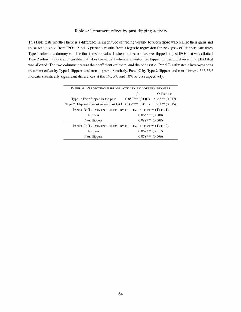
Table 4: Treatment effect by past flipping activity

This table tests whether there is a difference in magnitude of trading volume between those who realize their gains andthose who do not, from IPOs. Panel A presents results from a logistic regression for two types of “flipper” variables.Type 1 refers to a dummy variable that takes the value 1 when an investor has ever flipped in past IPOs that was allotted.Type 2 refers to a dummy variable that takes the value 1 when an investor has flipped in their most recent past IPO thatwas allotted. The two columns present the coefficient estimate, and the odds ratio. Panel B estimates a heterogeneoustreatment effect by Type 1 flippers, and non-flippers. Similarly, Panel C by Type 2 flippers and non-flippers. ***,**,*indicate statistically significant differences at the 1%, 5% and 10% levels respectively.

PANEL A: PREDICTING FLIPPING ACTIVITY BY LOTTERY WINNERS

b Odds ratioType 1: Ever flipped in the past 0.859*** (0.007) 2.36*** (0.017)

Type 2: Flipped in most recent past IPO 0.304*** (0.011) 1.35*** (0.015)PANEL B: TREATMENT EFFECT BY FLIPPING ACTIVITY (TYPE 1)

Flippers 0.065*** (0.008)Non-flippers 0.088*** (0.008)

PANEL C: TREATMENT EFFECT BY FLIPPING ACTIVITY (TYPE 2)Flippers 0.069*** (0.017)

Non-flippers 0.078*** (0.006)

64

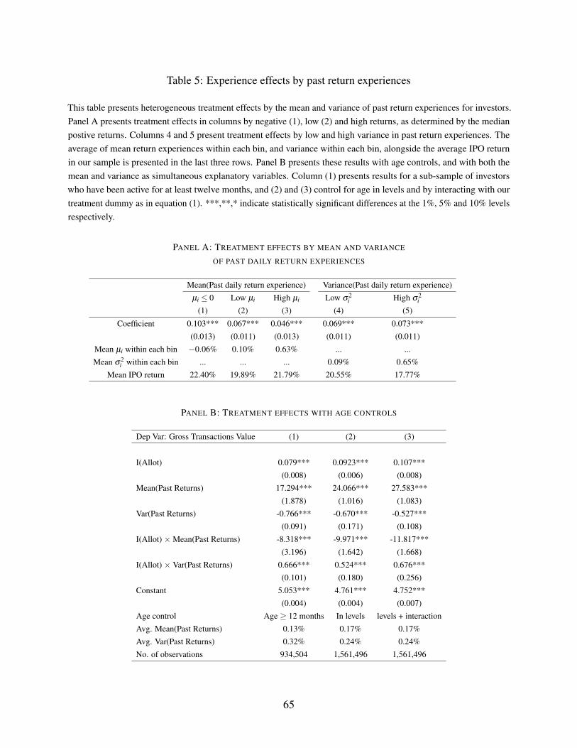
Table 5: Experience effects by past return experiences

This table presents heterogeneous treatment effects by the mean and variance of past return experiences for investors.Panel A presents treatment effects in columns by negative (1), low (2) and high returns, as determined by the medianpostive returns. Columns 4 and 5 present treatment effects by low and high variance in past return experiences. Theaverage of mean return experiences within each bin, and variance within each bin, alongside the average IPO returnin our sample is presented in the last three rows. Panel B presents these results with age controls, and with both themean and variance as simultaneous explanatory variables. Column (1) presents results for a sub-sample of investorswho have been active for at least twelve months, and (2) and (3) control for age in levels and by interacting with ourtreatment dummy as in equation (1). ***,**,* indicate statistically significant differences at the 1%, 5% and 10% levelsrespectively.

PANEL A: TREATMENT EFFECTS BY MEAN AND VARIANCE

OF PAST DAILY RETURN EXPERIENCES

Mean(Past daily return experience) Variance(Past daily return experience)µi 0 Low µi High µi Low s2

iHigh s2

i

(1) (2) (3) (4) (5)Coefficient 0.103*** 0.067*** 0.046*** 0.069*** 0.073***

(0.013) (0.011) (0.013) (0.011) (0.011)Mean µi within each bin �0.06% 0.10% 0.63% ... ...Mean s2

iwithin each bin ... ... ... 0.09% 0.65%

Mean IPO return 22.40% 19.89% 21.79% 20.55% 17.77%

PANEL B: TREATMENT EFFECTS WITH AGE CONTROLS

Dep Var: Gross Transactions Value (1) (2) (3)

I(Allot) 0.079*** 0.0923*** 0.107***(0.008) (0.006) (0.008)

Mean(Past Returns) 17.294*** 24.066*** 27.583***(1.878) (1.016) (1.083)

Var(Past Returns) -0.766*** -0.670*** -0.527***(0.091) (0.171) (0.108)

I(Allot) ⇥ Mean(Past Returns) -8.318*** -9.971*** -11.817***(3.196) (1.642) (1.668)

I(Allot) ⇥ Var(Past Returns) 0.666*** 0.524*** 0.676***(0.101) (0.180) (0.256)

Constant 5.053*** 4.761*** 4.752***(0.004) (0.004) (0.007)

Age control Age � 12 months In levels levels + interactionAvg. Mean(Past Returns) 0.13% 0.17% 0.17%Avg. Var(Past Returns) 0.32% 0.24% 0.24%No. of observations 934,504 1,561,496 1,561,496

65

Online AppendixLearning from Noise: Evidence from India’s IPO Lotteries

Santosh Anagol⇤ Vimal Balasubramaniam† Tarun Ramadorai‡

March 7, 2019

Contents

1 An Example: Barak Valley Cements IPO Allocation Process ii

2 Randomized and Non-Randomized Return Experiences iii

3 Bayesian Learning From Noise: Multiple risky-assets vi3.1 Learning about the distribution of market returns . . . . . . . . . . . . . . . . . . . vii3.2 Learning about own ability . . . . . . . . . . . . . . . . . . . . . . . . . . . . . . . viii

4 Empirical Appendix x

List of FiguresA.1 IPO FREQUENCY . . . . . . . . . . . . . . . . . . . . . . . . . . . . . . . . . . . . . . . . . . . . . . . xivA.2 IPO EXPERIENCE . . . . . . . . . . . . . . . . . . . . . . . . . . . . . . . . . . . . . . . . . . . . . . xvA.3 TOTAL RETAIL TURNOVER IN THE INDIAN STOCK MARKET . . . . . . . . . . . . . . . . . . . . . . . xviA.4 COMPARISON OF LOTTERY SAMPLE TO INDIA AND THE UNITED STATES . . . . . . . . . . . . . . . . xviiA.5 RETURN EXPERIENCE ACROSS EXPERIENCE BINS . . . . . . . . . . . . . . . . . . . . . . . . . . . . . xviiiA.6 TREATMENT EFFECT BY PAST TRADING ACTIVITY . . . . . . . . . . . . . . . . . . . . . . . . . . . . xixA.7 DAILY RETURNS DISTRIBUTION: INDIAN STOCKS 2002 � 2012 . . . . . . . . . . . . . . . . . . . . . xix

List of TablesA.1 Return experience and trading volume: Randomized vs. Non-Randomized Estimates . . . . . . . . . . . ivA.2 EXAMPLE IPO ALLOCATION PROCESS: BARAK VALLEY CEMENT IPO ALLOCATION . . . . . . . . . xA.3 Experience effects for Negative Return IPOs . . . . . . . . . . . . . . . . . . . . . . . . . . . . . . . . . xiA.4 GROSS TRANSACTION VALUE DECOMPOSITION BY PURCHASE AND SALE VALUE, AND IPO SECTOR xiiA.5 STATISTICAL TESTS FOR DIFFERENCES IN MAGNITUDES . . . . . . . . . . . . . . . . . . . . . . . . . xiii⇤Anagol: Wharton School of Business, Business Economics and Public Policy Department, University of Pennsylva-

nia. Email: anagol@wharton.upenn.edu†Balasubramaniam: Warwick Business School, University of Warwick, Scarman Road, Coventry CV4 7AL, UK.

Email: vimal.balasubramaniam@wbs.ac.uk‡(Corresponding author) Ramadorai: Imperial College London, and CEPR. Email: t.ramadorai@imperial.ac.uk

i

1 An Example: Barak Valley Cements IPO Allocation ProcessBarak Valley Cements’ IPO opened for subscription for the two day period October 29, 2007 through

November 1, 2007. The stock was simultaneously listed on the National Stock Exchange (NSE) and

the Bombay Stock Exchange (BSE) on November 23, 2007. The price that lottery winners paid for

the stock, which we refer to as the “issue price” throughout the paper, was Rs. 42 per share. The

price the stock first traded at on the market, which we we refer to as the “listing price,” was 62 rupees

per share. The stock closed on the first day of listing at 56.05 rupees per share, for a 33.45% listing

day gain (note that this gain is the positive shock experienced by those investors randomly allotted

the IPO shares, as we describe more fully below). The retail oversubscription rate v for this issue was

37.62. Given this high v, all retail investors that applied for this IPO were entered into a lottery.

Appendix Table A.1 shows the official retail investor IPO allocation data for Barak Valley Ce-

ments.1 Each row of column (0) of the table shows the share category c, associated with a number of

shares applied for given in column (1), which, given the minimum lot size x = 150 for this offer is just

cx. In this case, the total number of share categories (C) equals 15, meaning that the maximum retail

bid is for 2,250 shares.2 Column (2) of the table shows the total number of retail investor applications

received for each share category, and column (3) is the product of columns (1) and (2). Column (4)

shows the investor allocation under a proportional allocation rule, i.e., cxv . Given that these propor-

tional allocations are all below the minimum lot size of 150 shares, regulation requires the firm to

conduct a lottery to decide share allocations.

Column (5) shows the probability of winning the lottery for each share category c, which is p = cv .

For example, 2.7% of investors that applied for the minimum lot size of 150 shares will receive this

allocation, and the remaining 97.3% of investors applying in this share category will receive no shares.

In contrast, 40.6% of investors in share category c = 15 receive the minimum lot size x = 150 shares.

For this particular IPO, all retail investors are entered into a lottery, and ultimately receive either zero

or 150 shares of the IPO. Column (6) shows the total number of shares ultimately allotted to investors1These data are obtained from http://www.chittorgarh.com/ipo/ipo_boa.asp?a=134.2The number of share categories is capped at 15 here because C = 16 would correspond to 2,400 shares, and a

subscription amount of Rs. 100,800 at the issue price of Rs. 42. This subscription amount would violate the prevailing(in 2007) regulatory maximum retail investor application constraint of Rs. 100,000 rupees per IPO.

ii

in each share category, which is the product of x, column (2), and column (5). Columns (7) and

(8) show the total sizes of the winner and loser groups in each share category for the Barak Valley

Cements IPO lottery, respectively.

It is perhaps easiest to think of our data as comprising a large number of experiments, in which

each experiment is a share category within an IPO. Within each experiment the probability of treatment

is the same for all applicants, and we exploit this source of randomness, combining all of these

experiments together to estimate the causal effect of randomly experiencing the IPO listing return

on future investment behavior. We explain this more fully in the methodology section, following the

data description below.

2 Randomized and Non-Randomized Return ExperiencesTo conduct this comparison between randomized and non-randomized variation in return experiences,

we use two measures of non-randomized return experiences. The first is past returns on investors’

entire portfolios for all investors in the sample. The second is the returns experienced on the purchase

of the most recently selected stock for those investors who made exactly one purchase.

We first draw a 10% random sample from the universe of CDSL investor accounts, observed over

120 months. To explain the outcome of interest y, we then estimate:

yi,t = µi +wt + gRetExpi,t�1 +Xi,t�10b + ei,t (1)

Here, µi are individual fixed effects, wt are calendar month fixed effects, RetExpi,t�1 is a mea-

sure of the previous month’s experienced return, and Xi,t�1 are investor level controls lagged by one

month. The coefficient g is the experience effect estimated using traditional, non-randomized return

experience.

Column 2 of Table A.1 shows results when the measure of experienced returns are the portfolio

returns earned by investor i at the end of month t �1. Column 5 of the table shows results when the

sample is restricted to investors who purchased exactly one stock in month t � 1, meaning that the

measure of experience is the returns on this purchased stock.

iii

Table A.1: Return experience and trading volume:Randomized vs. Non-Randomized Estimates

This table presents a comparison of experience effects estimates using randomized variation in returns experience fromour main empirical specification (equation 1) (columns 1 and 4), with traditional measures of past returns experience suchas portfolio returns (columns 2 and 4) and for a sample of investors who purchased exactly one stock in month t (“Purchasereturns”, columns 3 and 6). Panel A presents the estimates with no additional control variables, without (columns 1–3) andwith (columns 4–6) calendar month fixed-effects. Panel (B) presents the same specification as in Panel (A) with additionalcontrols, including individual fixed-effects. The coefficient for randomized returns (columns 1 and 4) are normalized bymean IPO returns of 42% for comparison, at the end of first full month after listing. Columns 2,3,5 and 6 are estimatedon a 10% random sample from the universe of CDSL investors, observed over 120 months. Robust standard errors inparentheses, and ***,**,* represent statistical significance at 1%, 5% and 10% respectively.

(1) (2) (3) (4) (5) (6)Randomized Portfolio Purchase Randomized Portfolio Purchasereturns returns returns returns returns returns

Panel A: ”Raw” estimatesExperience effect 0.0018*** 0.0049*** 0.0120*** 0.0018*** 0.0040*** 0.0012***

(0.006) (0.000) (0.000) (0.005) (0.000) (0.000)IPO ⇥ Share category Fixed Effects Yes No No Yes No NoCalendar-Month Fixed Effects No No No No Yes Yes

Panel B: Estimates with additional controlsExperience effect 0.0018*** 0.0037*** 0.0021*** 0.0018*** 0.0036*** 0.0023***

(0.005) (0.000) (0.000) (0.005) (0.000) (0.000)IPO ⇥ Share category Fixed Effects Yes No No Yes No NoTime fixed effects No Yes Yes No Yes YesIndividual fixed effects No Yes Yes No Yes YesControl variables (lagged)

Portfolio size No No No Yes Yes YesTrading volume No No No Yes Yes YesAge No No No Yes Yes YesNo. of securities held No No No Yes Yes Yes

N 1,473,073 2,337,002 2,337,002 1,473,073 2,337,002 2,337,002

iv

Panel (A) of Table A.1 presents the estimates of the above regression without including controls

X on the right-hand side, while Panel (B) adds controls measured with a one-month lag. These

controls include portfolio size, trading value, time elapsed since the account was opened (age), and

the number of securities in the portfolio. In some specifications for non-randomized returns, we also

add individual-specific fixed effects.3 As the results are not particularly sensitive to the introduction

of these controls, we mainly discuss Panel (A) below.

In both panels of the table, Columns 1 and 4 just reproduce our main results using randomized

experienced returns to predict the inverse-hyperbolic sine of trading volume in the first full month

after the IPO.4 This is to facilitate ease of comparison between randomized and non-randomized

experience effects.

In Panel (A), Columns 1� 3 do not include calendar-month fixed-effects, while Columns 4� 6

of Panel (A) add calendar-month fixed-effects to the right-hand side. For the randomized return

experiences (moving from Column 1 to Column 4), the inclusion of these fixed effects has little

effect, because the main variation of interest happens within a given IPO (which only happens at

one time). In contrast, the inclusion of calendar-month fixed effects causes a very large difference

when experience is measured using non-randomized returns. The estimated effects reduce by about

18% following the inclusion of time fixed effects when portfolio returns are the experienced return

measure, and by a substantial margin of 90% when the single-stock purchase return is the experience

measure.

It is perhaps not surprising that the portfolio spillover effects of non-experimental returns are

highly sensitive to the inclusion of time fixed effects; any common factors driving returns will con-

found the estimate of experienced return effects, which the time fixed-effects will clear up. The

advantage of the experimental variation in returns delivered by the IPO lotteries is that it enables

portfolio spillover effects to be estimated without such confounds affecting inferences.

3We do not add these for the randomized returns, given that many individuals participate in only one lottery, andincluding them may eliminate the treatment-control balance induced by the experiment. We do analyze how the behaviorof participants varies conditional on the number of lotteries in which they participated in our subsequent analysis, to betterunderstand mechanisms of learning.

4The difference in magnitudes here arises from a scaling factor. To make this specification comparable to the otherswhere a continuous return variable is used, we divide the treatment effect of winning the lottery by 42%, as this is theweighted average return on our IPO lotteries.

v

To compare the point estimates from the randomized and non-randomized return experiences, we

turn to Columns 4� 6 of Panel (B). The experience effect looks quite different depending on the

method of estimation. It is perhaps fairest to compare the magnitudes of the single stock purchase

results (Column 6) with the randomized return experience (Column 4). Here, we can see that the point

estimate for the experience is roughly 28% higher for the non-randomized experience measure than

that generated by the experimental variation.

Though the estimate is higher for the non-randomized experience measure, the main takeaway is

that the two estimates are actually fairly close. This is reassuring, given the many possible differ-

ences between the types of experience associated with randomized and non-randomized experience

measures. Perhaps a good takeaway from this analysis is that it may be reasonable to assume that

selection effects or equilibrium considerations should not much affect inferences about investor re-

sponses to experienced returns.

3 Bayesian Learning From Noise: Multiple risky-assetsConsider an agent maximizing exponential utility �exp(�gW ) of terminal wealth W , with risk aver-

sion coefficient g .

maxq

�exp(�gW ) (2)

s.t.W = r f (W0 � iq)+qz (3)

The agent has to allocate initial wealth W0 between a risk-free asset with return r f , and a risky

asset vector with prices normalized to 1, delivering a random payoff vector of z. The choice variable

is q, the vector of amounts invested in the risky asset. i is a row vector of ones.

The agent does not know the true distribution of the risk asset payoff vector z; he begins with

a prior distribution and then updates to a posterior distribution based on signals (return experiences,

winning the IPO lottery, etc.). We call the prior distribution of the risky asset payoff r and assume that

this prior distribution is jointly normal with mean payoff vector r0 and variance-covariance matrix S0

(i.e. r ⇠ N(r0,S0)). Maximizing utility subject to the prior distribution of asset returns, the optimal

vi

portfolio allocation vector q⇤ = 1g S�1

0 (r0�r f ) =1g L0(r0�r f ), where L0 = S�1

0 is the precision matrix

of the agent’s priors about risky asset returns.

3.1 Learning about the distribution of market returns

The first case that we consider is that agents randomly experiencing gains or losses interpret this as a

signal about returns, whereas lottery losing agents that do not experience these returns act as if they

receive no signal. We denote the signal by s⇠N(r,Se), where Se =L�1e is a matrix of noise variances

and covariances associated with incoming signals.

If this were the case, following the IPO win, treated agents would use Bayes’ rule to calculate the

posterior distribution of returns. SS denotes the posterior variance-covariance matrix of returns, and

rS the posterior mean returns:

SS = S0(S0 +Se)�1Se ,LS = S�1

S . (4)

rS = S0(S0 +Se)�1s+(S0 +Se)

�1Se r0. (5)

Agents would adjust their portfolio to q⇤S = 1g LS(rS � r f ). We can generically consider two po-

tential types of signals. The first is that agents perceive the randomly experienced gains as a sign of

returns on the market. Equivalently, this is a rise in the expected returns of all stocks, i.e., all elements

of rS�r f are positive. The second type of perceived signal is more restricted, to particular stocks (say

those in the sector of the treatment IPO). In this case, some elements of rS � r f are positive, while

others are zero.

In the first case, i.e. a perceived rise in the expected return of all stocks, all elements of q⇤S

should be greater than the corresponding elements of q⇤ as a result of the mean return expectation on

risky assets increasing. Moreover, since the agents’ perceived posterior total precision LS is larger

following the signal, this provides an additional upward kick to q⇤S.

In the second case, i.e., a rise in the perceived expected return of some stocks, some elements of q⇤S

should be greater than the corresponding elements of q⇤, and the agent’s perceived posterior precision

LS is also greater, albeit for only some elements of the matrix.

vii

In both cases, the model yields counterfactual predictions. This is for two reasons. First, as we

know, the average allocation to risky assets for the treated does not rise — and this is predicted by

both types of signals about returns. It is true that a more restricted perceived signal does help to

explain the tilt towards particular sectors, but without a corresponding reduction in the means of other

sectors, or indeed an auxiliary assumption such as mental accounting, it is difficult to rationalize the

observed lack of an increase in the overall portfolio weight to risky assets. The second counterfactual

prediction is perhaps more troubling. Since the agent’s posterior precision LS is higher following the

perceived signal, we should observe that treated agents’ portfolio weights q⇤S react less to any future

incoming signals of either direction, assuming that the post-IPO signal distribution is balanced across

treated and control agents.5 This would predict a drop in future trading volume for the treated agents,

regardless of whether the initial signal was perceived to be positive or negative. This runs strongly

counter to our empirical results.6

3.2 Learning about own ability

We next consider the case in which the agent perceives the randomly experienced gains or losses from

the IPO as a positive or negative shock to their own investment ability.

To do so, we assume that a sensible measure of the agent’s ability is the precision of the signal

distribution, i.e., Le . The greater the signal precision, the greater the agent’s ability. This is a common

assumption in the literature on stock trading (see, for e.g., Gervais and Odean 2001, and Linnainmaa,

2011).

To model agents drawing inferences about their own ability, we consider agents with priors over

Le ⇠ Wishart(n ,L0e), where n is the number of observations about own ability that the agent has

previously experienced. If the treated agent updates their prior about their own ability in response

to a randomly experienced gain (essentially, treating experienced luck as a signal of their own skill),

then the agent will update perceived signal precision as LSe , with some of its elements increasing or

5Intuition is provided by the single risky asset case. If the treated agent’s posterior precision is rS, and the controlagent’s is r , and rS > r , any incoming signal with precision re about returns will be weighted re

rS< re

r by the treatedagent, affecting the distribution of portfolio weights less. This is the standard result about additional informational updatesaffecting posteriors marginally less.

6We note also that any interpretation of the IPO lottery as a shock to the precision of the market return distributionalso delivers the same (counterfactual) implication that the winners will be less responsive to all future signals.

viii

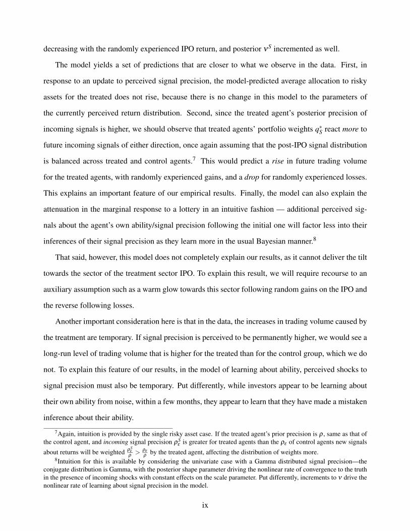
decreasing with the randomly experienced IPO return, and posterior nS incremented as well.

The model yields a set of predictions that are closer to what we observe in the data. First, in

response to an update to perceived signal precision, the model-predicted average allocation to risky

assets for the treated does not rise, because there is no change in this model to the parameters of

the currently perceived return distribution. Second, since the treated agent’s posterior precision of

incoming signals is higher, we should observe that treated agents’ portfolio weights q⇤S react more to

future incoming signals of either direction, once again assuming that the post-IPO signal distribution

is balanced across treated and control agents.7 This would predict a rise in future trading volume

for the treated agents, with randomly experienced gains, and a drop for randomly experienced losses.

This explains an important feature of our empirical results. Finally, the model can also explain the

attenuation in the marginal response to a lottery in an intuitive fashion — additional perceived sig-

nals about the agent’s own ability/signal precision following the initial one will factor less into their

inferences of their signal precision as they learn more in the usual Bayesian manner.8

That said, however, this model does not completely explain our results, as it cannot deliver the tilt

towards the sector of the treatment sector IPO. To explain this result, we will require recourse to an

auxiliary assumption such as a warm glow towards this sector following random gains on the IPO and

the reverse following losses.

Another important consideration here is that in the data, the increases in trading volume caused by

the treatment are temporary. If signal precision is perceived to be permanently higher, we would see a

long-run level of trading volume that is higher for the treated than for the control group, which we do

not. To explain this feature of our results, in the model of learning about ability, perceived shocks to

signal precision must also be temporary. Put differently, while investors appear to be learning about

their own ability from noise, within a few months, they appear to learn that they have made a mistaken

inference about their ability.

7Again, intuition is provided by the single risky asset case. If the treated agent’s prior precision is r , same as that ofthe control agent, and incoming signal precision rS

e is greater for treated agents than the re of control agents new signalsabout returns will be weighted rS

er > re

r by the treated agent, affecting the distribution of weights more.8Intuition for this is available by considering the univariate case with a Gamma distributed signal precision—the

conjugate distribution is Gamma, with the posterior shape parameter driving the nonlinear rate of convergence to the truthin the presence of incoming shocks with constant effects on the scale parameter. Put differently, increments to n drive thenonlinear rate of learning about signal precision in the model.

ix

4 Empirical Appendix

Table A.2: EXAMPLE IPO ALLOCATION PROCESS: BARAK VALLEY CEMENT IPO ALLOCATION

Share Category Shares Bid For # Applications Total Shares Proportional Allocation Win Probability Shares Allocated # Treatment group # Control group(c) (c⇥ x) ac ac ⇥ c⇥ x cx

vcv

cv ⇥ac (1� c

v)⇥ac

(0) (1) (2) (3) (4) (5) (6) (7) (8)1 150 14,052 2,107,800 4 0.027 57,000 380 13,6722 300 9,893 2,967,900 8 0.054 80,250 535 9,3583 450 5,096 2,293,200 12 0.081 61,950 414 4,6824 600 4,850 2,910,000 16 0.108 78,750 525 4,3255 750 2,254 1,690,500 20 0.135 45,750 305 1,9496 900 1,871 1,663,900 24 0.162 45,450 304 1,5677 1050 4,806 5,046,300 28 0.189 136,500 910 3,8968 1200 2,900 3,480,000 32 0.216 94,050 628 2,2729 1350 481 649,350 36 0.244 17,550 117 36410 1500 1,302 1,953,000 41 0.271 52,800 352 95011 1650 266 436,900 45 0.298 11,850 79 18712 1800 317 570,600 49 0.325 15,450 103 21413 1950 174 339,300 53 0.352 9,150 61 11314 2100 356 747,600 57 0.379 20,250 135 22115 2250 20,004 45,009,000 61 0.406 1,217,700 8119 11,885Note: Columns (7) and (8) are obtained after applying the regulation defined rounding off methodology as described in the Online Appendix to Anagol, Balasubramaniam and Ramadorai (2018).

x

Table A.3: Experience effects for Negative Return IPOs

Event-time-1 0 1 2 3 4 5 6

1. Future IPO 0.0041 0.0010 -0.0055* -0.0071** -0.0018 -0.0045** -0.0068*** -0.0023*participation (0.0034) (0.0030) (0.0030) (0.0034) (0.0021) (0.0020) (0.0024) (0.0012)

2. Gross transaction 0.0001 -0.0050 -0.0048 -0.0585** -0.0469* 0.0044 -0.0493** -0.0640**value (0.0249) (0.0238) (0.0225) (0.0266) (0.0276) (0.0278) (0.0250) (0.0265)

3. Gross transaction 0.0008 -0.0039 -0.0037 -0.0574* -0.0458** 0.0054 -0.0482* -0.0628**value / Portfolio value (t-1) (0.0064) (0.0267) (0.0285) (0.0309) (0.0215) (0.0319) (0.0281) (0.0306)

4. Gross No. of -0.0032 -0.0013 -0.0075 -0.0179** -0.0079 -0.0009 -0.0135* -0.0098Transactions (0.0084) (0.0083) (0.0078) (0.0081) (0.0080) (0.0081) (0.0076) (0.0078)

5. Weight in IPO sector -0.0001 0.0007 -0.0001 -0.0004 -0.0006 -0.0006 -0.0009 -0.0013(0.0009) (0.0012) (0.0009) (0.0009) (0.0009) (0.0009) (0.0009) (0.0009)

6. Portfolio value -0.0011 -0.0135 0.0062 -0.0048 -0.0063 0.0112 0.0093 -0.0128(0.0236) (0.0216) (0.0209) (0.0214) (0.0220) (0.0224) (0.0225) (0.0232)

xi

Table A.4: GROSS TRANSACTION VALUE DECOMPOSITIONBY PURCHASE AND SALE VALUE, AND IPO SECTOR

Gross Transactions ValueEvent time Purchase value Sale value Non-IPO Sector IPO Sector

-3 0 0.004 0.006 0.004-2 -0.002 0.008 0.007 -0.002-1 0.007 0.01 0.009 0.0040 0.011* 0.027*** 0.021*** 0.015***1 0.063*** 0.069*** 0.057*** 0.068***2 0.057*** 0.058*** 0.048*** 0.047***3 0.037*** 0.032*** 0.025*** 0.033***4 0.023*** 0.029*** 0.028*** 0.020***5 0.022*** 0.030*** 0.019*** 0.023***6 0.023*** 0.026*** 0.024*** 0.017***

xii

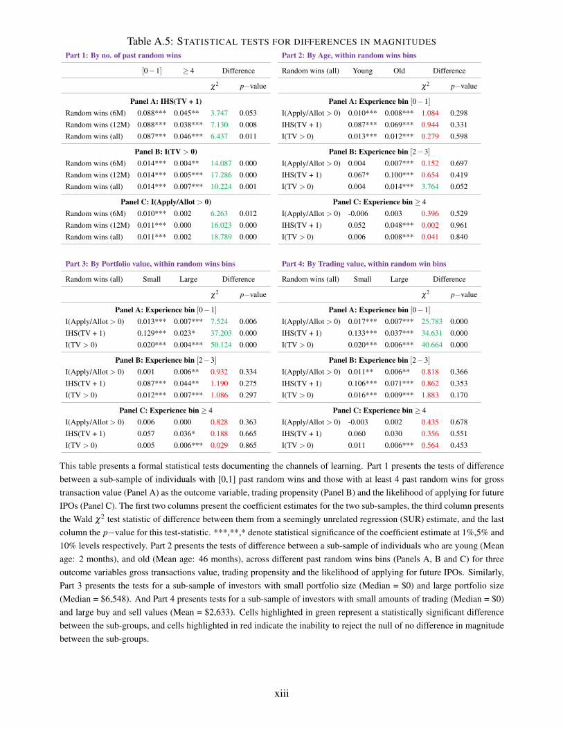
Table A.5: STATISTICAL TESTS FOR DIFFERENCES IN MAGNITUDESPart 1: By no. of past random wins Part 2: By Age, within random wins bins

[0�1] � 4 Difference Random wins (all) Young Old Difference

c2 p�value c2 p�value

Panel A: IHS(TV + 1) Panel A: Experience bin [0�1]Random wins (6M) 0.088*** 0.045** 3.747 0.053 I(Apply/Allot > 0) 0.010*** 0.008*** 1.084 0.298Random wins (12M) 0.088*** 0.038*** 7.130 0.008 IHS(TV + 1) 0.087*** 0.069*** 0.944 0.331Random wins (all) 0.087*** 0.046*** 6.437 0.011 I(TV > 0) 0.013*** 0.012*** 0.279 0.598

Panel B: I(TV > 0) Panel B: Experience bin [2�3]Random wins (6M) 0.014*** 0.004** 14.087 0.000 I(Apply/Allot > 0) 0.004 0.007*** 0.152 0.697Random wins (12M) 0.014*** 0.005*** 17.286 0.000 IHS(TV + 1) 0.067* 0.100*** 0.654 0.419Random wins (all) 0.014*** 0.007*** 10.224 0.001 I(TV > 0) 0.004 0.014*** 3.764 0.052

Panel C: I(Apply/Allot > 0) Panel C: Experience bin � 4Random wins (6M) 0.010*** 0.002 6.263 0.012 I(Apply/Allot > 0) -0.006 0.003 0.396 0.529Random wins (12M) 0.011*** 0.000 16.023 0.000 IHS(TV + 1) 0.052 0.048*** 0.002 0.961Random wins (all) 0.011*** 0.002 18.789 0.000 I(TV > 0) 0.006 0.008*** 0.041 0.840

Part 3: By Portfolio value, within random wins bins Part 4: By Trading value, within random win bins

Random wins (all) Small Large Difference Random wins (all) Small Large Difference

c2 p�value c2 p�value

Panel A: Experience bin [0�1] Panel A: Experience bin [0�1]I(Apply/Allot > 0) 0.013*** 0.007*** 7.524 0.006 I(Apply/Allot > 0) 0.017*** 0.007*** 25.783 0.000IHS(TV + 1) 0.129*** 0.023* 37.203 0.000 IHS(TV + 1) 0.133*** 0.037*** 34.631 0.000I(TV > 0) 0.020*** 0.004*** 50.124 0.000 I(TV > 0) 0.020*** 0.006*** 40.664 0.000

Panel B: Experience bin [2�3] Panel B: Experience bin [2�3]I(Apply/Allot > 0) 0.001 0.006** 0.932 0.334 I(Apply/Allot > 0) 0.011** 0.006** 0.818 0.366IHS(TV + 1) 0.087*** 0.044** 1.190 0.275 IHS(TV + 1) 0.106*** 0.071*** 0.862 0.353I(TV > 0) 0.012*** 0.007*** 1.086 0.297 I(TV > 0) 0.016*** 0.009*** 1.883 0.170

Panel C: Experience bin � 4 Panel C: Experience bin � 4I(Apply/Allot > 0) 0.006 0.000 0.828 0.363 I(Apply/Allot > 0) -0.003 0.002 0.435 0.678IHS(TV + 1) 0.057 0.036* 0.188 0.665 IHS(TV + 1) 0.060 0.030 0.356 0.551I(TV > 0) 0.005 0.006*** 0.029 0.865 I(TV > 0) 0.011 0.006*** 0.564 0.453

This table presents a formal statistical tests documenting the channels of learning. Part 1 presents the tests of differencebetween a sub-sample of individuals with [0,1] past random wins and those with at least 4 past random wins for grosstransaction value (Panel A) as the outcome variable, trading propensity (Panel B) and the likelihood of applying for futureIPOs (Panel C). The first two columns present the coefficient estimates for the two sub-samples, the third column presentsthe Wald c2 test statistic of difference between them from a seemingly unrelated regression (SUR) estimate, and the lastcolumn the p�value for this test-statistic. ***,**,* denote statistical significance of the coefficient estimate at 1%,5% and10% levels respectively. Part 2 presents the tests of difference between a sub-sample of individuals who are young (Meanage: 2 months), and old (Mean age: 46 months), across different past random wins bins (Panels A, B and C) for threeoutcome variables gross transactions value, trading propensity and the likelihood of applying for future IPOs. Similarly,Part 3 presents the tests for a sub-sample of investors with small portfolio size (Median = $0) and large portfolio size(Median = $6,548). And Part 4 presents tests for a sub-sample of investors with small amounts of trading (Median = $0)and large buy and sell values (Mean = $2,633). Cells highlighted in green represent a statistically significant differencebetween the sub-groups, and cells highlighted in red indicate the inability to reject the null of no difference in magnitudebetween the sub-groups.

xiii

Figure A.1: IPO FREQUENCY

OthersSample

No.

of I

POs

05

1015

20

Jan

2007

Mar

200

7M

ay 2

007

Jul 2

007

Sep

2007

Nov

200

7Ja

n 20

08M

ar 2

008

May

200

8Ju

l 200

8Se

p 20

08N

ov 2

008

Jan

2009

Mar

200

9M

ay 2

009

Jul 2

009

Sep

2009

Nov

200

9Ja

n 20

10M

ar 2

010

May

201

0Ju

l 201

0Se

p 20

10N

ov 2

010

Jan

2011

Mar

201

1M

ay 2

011

Jul 2

011

Sep

2011

Nov

201

1

xiv

Figure A.2: IPO EXPERIENCE

First-day returns

2007 2008 2009 2010 2011

−50

050

100

150

First day

:

(Closing

Price

Issue Price

−1)100

●

●

●

●

●

●

●

●

●

●

●

●

●

●

●

●●

●

●

●

●

●

●

●

●

●

●

●●

●

●

●

●●

●●

●

●

●

●●

●

●

●

●●

●

●

●

●

●

●

●

●

[12] [10] [2] [22] [8]

Mean

First-day returns variability

2007 2008 2009 2010 2011

020

4060

80100

120

140

First day

:

High −

Low

Issue Price10

0

●

●

●

●

●

●

●

●●

●

●

● ●

●

●

●

●

●

●●●

●

●

●

●

●

●

●

●●

●

●

●

●

●

●

●

●●

●

●

●

●

●

●●

●

●

●

●

●

●

●

●

[12] [10] [2] [22] [8]

Mean

xv

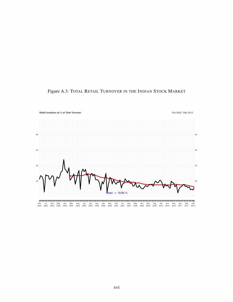
Figure A.3: TOTAL RETAIL TURNOVER IN THE INDIAN STOCK MARKET

Feb2002

Jul2002

Dec2002

May2003

Oct2003

Mar2004

Aug2004

Jan2005

Jun2005

Nov2005

Apr2006

Sep2006

Feb2007

Jul2007

Dec2007

May2008

Oct2008

Mar2009

Aug2009

Jan2010

Jun2010

Nov2010

Apr2011

Sep2011

Feb2012

Retail Investors as % of Total Turnover Feb 2002 / Mar 2012

20

40

60

80

20

40

60

80

Mean = 19.85 %

xvi

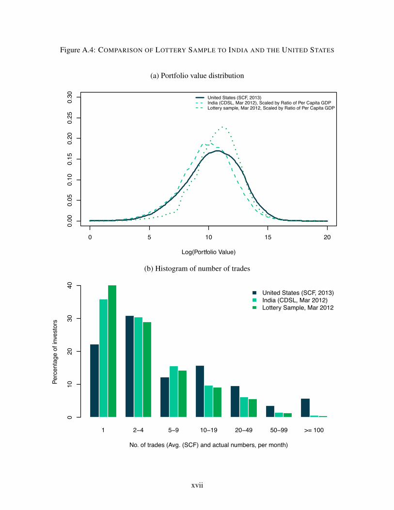
Figure A.4: COMPARISON OF LOTTERY SAMPLE TO INDIA AND THE UNITED STATES

(a) Portfolio value distribution

0 5 10 15 20

0.00

0.05

0.10

0.15

0.20

0.25

0.30

Log(Portfolio Value)

United States (SCF, 2013)India (CDSL, Mar 2012), Scaled by Ratio of Per Capita GDPLottery sample, Mar 2012, Scaled by Ratio of Per Capita GDP

(b) Histogram of number of trades

1 2−4 5−9 10−19 20−49 50−99 >= 100

No. of trades (Avg. (SCF) and actual numbers, per month)

Perc

enta

ge o

f inv

esto

rs

010

2030

40

United States (SCF, 2013)India (CDSL, Mar 2012)Lottery Sample, Mar 2012

xvii

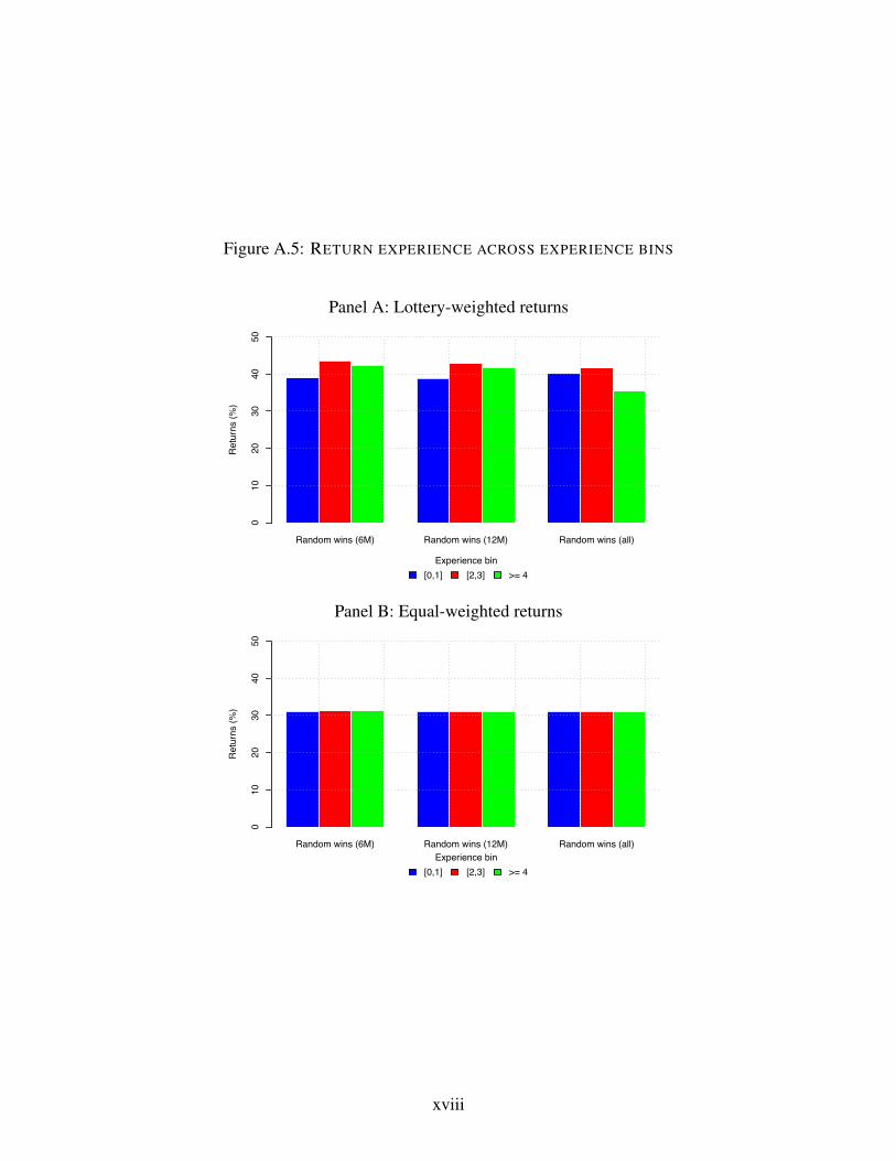
Figure A.5: RETURN EXPERIENCE ACROSS EXPERIENCE BINS

Panel A: Lottery-weighted returns

Random wins (6M) Random wins (12M) Random wins (all)

Ret

urns

(%)

010

2030

4050

Experience bin[0,1] [2,3] >= 4

Panel B: Equal-weighted returns

Random wins (6M) Random wins (12M) Random wins (all)

Ret

urns

(%)

010

2030

4050

Experience bin[0,1] [2,3] >= 4

xviii

Figure A.6: TREATMENT EFFECT BY PAST TRADING ACTIVITY

−0.0

40.

000.

020.

040.

060.

080.

10

[0,5] (5,10] (10,30] > 30

(1,295,438) (139,396) (97,732) (28,038)(1,295,438)No. Obs =

Figure A.7: DAILY RETURNS DISTRIBUTION:INDIAN STOCKS 2002 � 2012

Daily returns − Indian stocks 2002 − 2012

Den

sity

−0.4 −0.2 0.0 0.2 0.4

02

46

810

Mean = 0.16%

Variance = 0.25%

xix