Learning Edition Workbook - reference.digilentinc.com · Learning Edition Workbook Kaitlyn Franz, ... This workbook is designed to help you get started with electronics instrumentation

Learning EditionWorkbook

Kaitlyn Franz, Larissa Swanland,and Norman MacDonald

Getting started with your OpenScope MZthrough an introduction to analog circuits.

Learning EditionWorkbook

Getting started with your OpenScope MZthrough an introduction to analog circuits.

Kaitlyn Franz, Larissa Swanland,and Norman MacDonald

Introduction 3

Introduction

Thank you for backing the Learning Edition of the OpenScope MZ!

This workbook is designed to help you get started with electronics instrumentation. It assumes you have some rudimentary knowledge of electronic prototyping, but no prior experience with instru-mentation. The workbook is designed to briefly dip into various example circuits and highlight key instrumentation tools, all while providing the terminology and resources to learn more.

If you were expecting more of a “basics of electronics” experience, we highly recommend Charles Platt’s Make: Electronics book in order to learn the basics of breadboarding, prototyping, schematic reading, and component identification. If you know the basics of electronics but are trying to learn

4 Introduction

more, then we recommend as a companion to this workbook, Electrical Engineering 101: Everything You Should Have Learned in School...But Probably Didn’t by Darren Ashby. If you are already familiar with using tools such as oscilloscopes, waveform generators, logic analyzers, network analyzers, and power supplies, then consider this a refresher workbook. You will be particularly interested in the beginning sections explaining the OpenScope MZ and our design approach to the tool.

This workbook is laid out into three sections:

Part 1: What is instrumentation, and why do we need it? This is a general overview of the tools on the OpenScope MZ and will help you orient your-self around some key terms.

Part 2: The OpenScope MZ and WaveForms Live - your instrumentation tool.This section will cover setup and taking your first measurement.

Part 3: Let’s get hands-on!A selection of exercises to get you practicing with the OpenScope MZ and introducing you to some Analog Electronic concepts. These exercises were selected in order to give you the widest range of problems you may experience in your electronics journey. Solving these ex-ercises will help you get familiar with all of the OpenScope MZ tools, enabling the use in future projects. Some of them are based deep in theory, but rather than make the entire work-book theory-based, we’ve decided to provide an example and give you the terms and resources to learn more. Every exercise has additional information in a course that we previously made called Real Analog.

In order to follow along with the exercises, you will need to learn the following topics:

• How to use a breadboard• How to read resistor values• How to read capacitor values

We’ve included some handy guides in the appendix on each of these topics. There are also several YouTube tutorials that you can follow that will help you navigate these guides. You’ll find these tutorials listed in the appendix.

We hope you enjoy this workbook, and happy measuring!

Larissa, Kaitlyn and Norman

When asked what the OpenScope MZ is, we usually reply “instrumentation”. But what exactly is instrumentation? Consider some objects that most of you will be familiar with:

• A ruler is a measuring instrument: measures distance in inches or centimeters.

• A scale is a measuring instrument: measures weight in Kg or Lbs.

• A voltmeter is a measuring instrument: measures a single voltage level. (You use this every time you check a battery’s charge.)

• An oscilloscope is also a measuring instrument: measures voltage and plots it over time.

Any type of instrumentation is a tool that helps you quantify and see important values that dictate the function of your project.

For us, we are concerned with electronics instrumentation, or tools that help us see signals and values in electronics. A huge challenge in getting started with electronics is that the world of electronics is largely unseen. It’s often said that electronics instrumentation makes the invisible, visible. After all, electrons are both too small and too fast for us to observe with the naked eye. With modern electronics, there are additional complexities given how integrated (multiple types of electronics combined into a single space) and dense products are.

Part I: What is instrumentation and why do we need it? 5

Part 1:

What is instrumentation, and why do we need it?

6 Part I: What is instrumentation, when do we need it?

We often use the following analogy with new users to help them better understand electronics: Working on electronics projects is a lot like being a surgeon. When a surgeon sees the patient, they see the symptoms from the outside; they see a knee that doesn’t bend quite right or is causing pain. In your project, you may see a motor that doesn’t turn at quite the right speed or even turn at all. A surgeon will likely be able to guess what the problem is, and if they have a lot of experience they might even be correct on the first guess - just like you may be able to make an appropriate guess as to why the motor is malfunctioning. But just as a malfunctioning knee might be caused by the bone, the cartilage, or the muscle, your malfunctioning motor might be caused by the signals coming from your microcontroller, a fried pin on the microcontroller, a fried motor controller, or a broken motor itself. A surgeon will likely use X-rays or an MRI to see the unseen in their patient and determine the exact cause of the injury. The MRI and X-ray are the surgeon’s instruments. You can use an oscilloscope and logic analyzer to see the unseen in your project. First, you can look at the signals coming out of the microcontroller pins: do they seem correct, and are they even there? Then if those are right, look at those coming out of the motor controller: do they look right, and are they even there? You can even use a pattern generator to output the correct motor signals to test the functionality of your motor.

Sure, the surgeon could use exploratory surgery as the first diagnostic tool, but it’s more efficient to use instruments that were created to see the unseen and pinpoint the exact cause of the issue without having to waste time and money. In electronics, instruments can help you pinpoint the exact cause of a strange behavior, and teach you more about the functionality of your project. We have taken apart projects, replaced components, gone through the code, and ramped up our levels of stress and frustration only to take out a scope and discover that one of the pins was fried. What we learned was that taking out the scope should have been the first step.

Much like an X-ray or MRI, instruments help you see the signals that are causing the “symptoms” you see and will decrease the frustration and potential mistakes made during the process of diag-nosing and fixing the issue.

The following are the major tools that we use in electronics:

Prototyping tools: Soldering irons and simulators.

Sources: Power supplies and signal generators.

Meters: Voltmeters and DMMs (digital multimeters).

Scopes: Oscilloscope and analyzers.

Part I: What is instrumentation, when do we need it? 7

We’ve put together the following chart of tools and when to use them. Not all tools you will use are included on the chart, but we highlighted some important ones.

Name Type Explanation When to Use Notes

Soldering Iron

Prototyping To make permanent electrical connections using melted metal.

When you don’t want your components to move.

Hakko, generic ones from eBay, and Metcal are popular brands.

Simulator Prototyping A place to test out components or circuits virtually, like a test drive.

When you need to know the output of a circuit before you build. For example, you are worried about the cost or time spent building a prototype.

LT Spice and Multisim Live are some free simulators that are great for teaching.

PowerSupply

Sources Supplies a constant level of voltage or current. If it’s program-mable, it’s called a programmable power supply.

When you are told you need a certain voltage or current to operate a circuit, component, or project.

Batteries, USB battery packs, wall supplies, or a large benchtop power supply. These can range from a DIY computer power supply to expensive lab equipment.

WaveformGenerator

Sources This is essentially a power supply that has been programmed to output power in a specific pattern (e.g., sine wave, triangle wave, etc.).

When you need signals to stimulate a circuit, or want to ob-serve what happens in an alternating current/voltage situation.

Arbitrary Waveform Generators, Function Generators, or Signal Generators provide similar functionality.

Waveform generators can range from $40-$1800+

Multimeter /Voltmeter

Meters This measures and displays the voltage, current, and sometimes resistance wherever the probes are placed as a single number.

If it only measures voltage, it’s a voltmeter.

When you need to check that your circuit is connected or getting the correct values needed for operation. Best used with fixed power supplies (because the source isn’t changing). If you’ve ever used a battery tester, you’ve used a voltmeter!

You can get a cheap multimeter for under $10 at discount stores. Nicer ones will “auto range” and calculate your units for you.

8 Part I: What is instrumentation, when do we need it?

Name Type Explanation When to Use NotesOscilloscope Scope This measures voltage

and current over time (multiple points). It allows you to “draw” out what is happening with the circuit on a screen. This is best for analog circuits (where the signal isn’t just a high or low). If you took voltmeter mea-surements and plotted them in a graph over time, you would be an oscilloscope.

When you need to understand how your circuit is responding or changing.

You can get a cheap oscilloscope for about $60 or a large profes-sional one for $1500+. Things to notice are the number of channels, bandwidth, and sampling rate.

SpectrumAnalyzer

Scope This plots the amount of each frequency in a signal in a bar graph.

When you need to know what frequen-cies make up your signal (e.g., what is the message fre-quency (data) in your AM radio signal?).

Standalone spectrum analyzers can cost upwards of $20,000 and provide incredible accuracy. Many USB instrumentation devices contain simple spectrum analyzers that can help analyze most signals.

LogicAnalyzer

Scope Reads data as 1 or a 0 (digital), and plots it as a square wave. Depend-ing on the pattern of the pulses, a protocol can be determined and data can be displayed. Think of this tool as a “decoder”.

When you need to see the function of a digital signal such as SPI, I2C, or something going high or low, or when you need to see if data is being transferred correctly, i.e., is your light sensor sending the correct values?

These can range from a cheap $20-$30 microcontroller-based solution to one that is $300-$1000. It just depends on how fast and complicated your signals are.

Logger Scope(ish) Stores information from your scope or meters to a specific location over a long period of time.

When you need to ac-cess the data remotely, at a later time, or log data for long periods of time. Also useful if you need to read really slow signals and graph the points out later.

Data loggers are often tied to a specific sensor, or are bulky and expensive. A desktop datalogger can go for several thousand dollars, and many multi-function USB instrumentation devices contain basic data loggers that get the job done.

...table cont’d

Part 2: The OpenScope MZ and WaveForms Live - your instrumentation tool. 9

If you backed the Kickstarter campaign, you probably watched our video about the OpenScope MZ and have a general idea of what it does. Let’s go into a little more detail.

The OpenScope MZ is a microcontroller-based tool that was designed to turn your computer into an oscilloscope, waveform generator, power supply, simple logic analyzer, basic spectrum analyzer, and a data logger.

Part 2:The OpenScope MZ and WaveForms

Live - your instrumentation tool.

10 Part 2: The OpenScope MZ and WaveForms Live - your instrumentation tool.

So, here’s the setup:

A computer running WaveForms Live (the controlling and visualizing software) is connected to the OpenScope MZ, which does all of the signal generating and signal reading. The wires connect-ed to the OpenScope MZ are used to connect to a circuit. For a more detailed view, let’s take a look at the anatomy of an OpenScope MZ.

OpenScope MZ Specs

The OpenScope’s PIC32MZ microcontroller is the brains of the operation, while its MRF24 Wi-Fi Radio and Serial USB handle the communication between it and your computer. There are various analog circuits that convert the raw information from the flywires into something the microcontroller can digest.

Hardware features:

• 2 oscilloscope channels with 12 bits at 2MHz bandwidth and 6.25 MS/s max sampling rate.

• 1 function generator output with 1MHz bandwidth at 10 MS/s update rate.

• 10 user-programmable pins configurable as either GPIO or as a 10-channel logic analyzer.

• User-programmable power supplies supplying up to 50mA and ± 4V power.

• USB bus-powered or externally powered.

• On-board Wi-Fi.

• Browser-based WaveForms Live multi-instrument software.

• Re-programmable through Arduino IDE or Microchip MPLAB X IDE.


FirmwareThe firmware interacts with the hardware to create the instrument operation, maintain and run calibration, manage communication with USB and Wi-Fi, and storage.

WaveForms Live WaveForms Live is the browser-based user interface that allows you to interact with the Open-Scope locally or via Wi-Fi. It also takes the form of iOS and Android applications.

Digilent AgentThe Digilent Agent manages communication between your computer and the OpenScope MZ; making the connections, setting up the device, and communicating over USB or Wi-Fi.

Setting Up Your OpenScope MZ

Now that you know what your OpenScope is made of, let’s get set up and take a measurement!

Step 1: Make sure you have all the components in place

Before you begin, you’ll need:

• The OpenScope MZ

• A micro USB cable

• Your computer

• Some breadboard wires or staples (2)

Step 2: Download, install, and open the Digilent Agent

The Digilent Agent is a service that runs in the sys-tem tray on Windows, Mac and Linux and enables browser based applications to communicate with Digilent hardware.


• Go to: http://digilent.com/digilentagent

• Download the correct version for your computer

• Go to: www.waveformslive.com

• When you first go to WaveFormsLive.com, you’ll be taken directly to the device manager.

• Install the agent

Step 3: Start up WaveForms Live

...Step 2 cont’d


Step 4: Add your OpenScope MZ

• Click “Add Device”

• Select “Agent” then hit the ‘+’ button.


• Select serial port. If multiple serial ports are showing, you may have to try a few before you succeed.

Windows

Mac OS Linux

...Step 4 cont’d


• If this is the first time you are using your OpenScope MZ, WaveForms Live will prompt you to update the firmware:

• Click “OK”. This will take just a few moments:

• It is always advised that you choose the latest firmware in the event that new tools were added or optimized.

Step 5: Update the firmware


You may see a warning that your device is uncalibrated, at which point you’ll be taken to the calibration wizard.• Get two breadboard wires out of your Analog Parts Kit• Connect DCOUT1 (solid red wire) to OSC1 (solid orange wire)• Connect DCOUT2 (solid white wire) to OSC2 (solid blue wire)

• Click “Begin”. When prompted, save your new calibration information to the “flash” storage location and click “Done”:

• NOTE: While you are still in the configuration menu, take note of your device’s IP address: (You may need this later if you set up Wi-Fi.)

Step 6: Calibrate your OpenScope MZ


• Click the menu button in the top-left corner of the main window, then select “Device Manager”.

• In the Device Manager, click on the device tile for your OpenScope MZ.

• This will bring up the Instrument Panel.

Step 7: Take your first measurement

...Step 6 cont’d


• Note the “PIN” button in the instrument panel.

• This will bring up a useful pin-out diagram, showing you the flywire colors and signal names for your OpenScope MZ.

• Using the pin-out diagram for reference, use a breadboard wire to connect OSC1 to AWG1 (Oscilloscope channel 1 to Arbitrary Waveform Generator channel 1)

• Turn on the Waveform Generator.

Click on the power button to turn on the AWG. The button will turn from grey to blue. Note that Osc Ch1 is turned on by default.

...Step 7 cont’d


• Click “RUN”.

• You can now see the output from the AWG in the oscilloscope window. Try playing with some of the controls to see the resulting changes.

...Step 7 cont’d

Click to change how much time

is shown.

Click to change the voltage

range shown.

Click to move the waveform up and down.

Part 3: Let’s get hands-on! 21

Part 3:

Let’s get hands-on!

In this section, we’ll go through several exercises designed to introduce you to the world of ana-log circuits, teach some basic terminology, and help you familiarize yourself with the tools on the OpenScope MZ. But first, let’s dive into some details on the Analog Parts Kit. This kit will be your companion in this workbook. When we call out a component for an exercise, it will always come from the parts kit unless we explicitly state otherwise. This parts kit has over 160 individual components that includes ICs, amplifiers, sensors, resistors, potentiometers, capacitors, transistors, LEDs, diodes, inductors, and other miscellaneous components. This means this kit can easily work for beginners and experienced users. We’ll use two of the components of this kit in the following exercises.

22 Part 3: Let’s get hands-on!

Analog Parts Kit contents:

Part of getting into a new field or getting to use a new tool is learning the terminology and the basic concepts. One of the most basic concepts is Ohm’s Law.

Exercise 1: Ohm’s law

If you’ve been around electronics or heard any electrical engineer talk about circuits, you’ve prob-ably heard about something called Ohm’s Law. Ohm’s law is essentially the one equation that governs almost all electronics behavior, similar to how the laws of gravity govern much of what happens in the universe. Ohm’s law is:

V = IR

Inspired yet? Let me explain. V stands for voltage (measured in Volts), I stands for current (measured in Amps), and R stands for resistance (measured in Ohms). So, Voltage equals Current multiplied by Resistance. One of the most basic circuits is a voltage applied to a resistor, as seen in Figure 3-1.

Well, we generally know what voltage the power supply is providing, and we know what the resistor value should be based on the color code. But what if we wanted to know the current? We can find out with some manipulation of Ohm’s Law:

I = V/R

Not only can we define the voltage and resistance of our circuit, but we can also find out the current.

This becomes incredibly useful as you run into components that may have current limitations, or where their behavior changes with the current applied. In its original form, we can find the voltage if the current and resistance is known. And we can find the equivalent resistance of an unknown circuit if we know the current and voltage:

R = V/I

Ohm’s law is pretty simple, but it leads to some helpful circuit analysis when combined with Kirch-hoff ’s Voltage Law (KVL) and Kirchhoff ’s Current Law (KCL). These three laws are applied in Nodal and Mesh Analysis, which can be used to find the current and voltages at any point in a circuit. To learn more about any of the laws or circuit analysis techniques mentioned, check out Real Analog.

Now that you know Ohm’s Law, what about power?

Exercise 2: Let’s talk about power

Many circuit components or parts of a project have power limitations instead of current limitations. Sometimes those power limitations will prevent you from damaging a component, and sometimes they just define how much you can get from that particular source or component. Many people go

Figure 3-1 Simple circuit and schematic showing voltage applied to a resistor.



about their projects hoping that they don’t exceed these limitations, or struggle with a project un-aware that the unknown limitation is a power limitation.

There’s another important equation to define circuit behavior, this time it’s for power!

P = IV

Another simple but all-powerful equation (pun intended). This equation means that the voltage multiplied by the current equals the power. Let’s look at this in practice by checking out our simple resistor circuit.

We know the amount of voltage applied to the circuit from our power supply because we set that. We know the resistance based on the resistor color code, so we can determine the current from Ohm’s Law. Since we know the current and the voltage, we can determine the power dissipated across the resistor.

P = I 2R

For more information about power, check out Real Analog.

Now let’s get into some circuits that require the use of an oscilloscope.

Figure 3-2 Our simple resistor circuit.

Exercise 3: RC circuit response

So far all we’ve seen are voltages that could be measured with a DMM. Our circuits haven’t had any time-varying signals or time-varying components. Most circuits in electronics are not this simple. Either the signal will vary with time, or you might have some components with non-linear behavior, like capacitors. In the most basic sense, capacitors slowly collect charge and then slowly discharge over time. But what does that mean in terms of signals? Let’s find out!

We’ll need to build a basic RC circuit, comprised of a resistor and capacitor. You can see the values on the schematic below.

We’ll connect the waveform generator to one side of the resistor and oscilloscope channel 1 to the other side. Connect one side of the capacitor to the oscilloscope, and the other side to a ground.


Figure 3-3 A basic RC circuit.

Figure 3-4 Setting up our RC circuit.

Make sure your settings match the settings seen here.

Click “RUN” and you should see the signal pictured in Figure 3-6.

In electrical engineering terms, the first half of the signal with the trigger on it (the green line) is the Forced response and the second half is the Natural response. In other words, the first section shows the response of the circuit when you suddenly apply a voltage, e.g., the charging of the ca-pacitor. The second section shows the response of the circuit when you remove that voltage, e.g., the discharging of the capacitor.

There are of course a lot of equations and theory that govern the charging and discharging of ca-pacitors, but we won’t get into that here. If you are interested in learning more, Real Analog provides more information on the subject.


Figure 3-5 Setting up WaveForms Live for our RC circuit exercise.

Exercise 4: Take a moment to explore triggers

With the circuit from the previous exercise plugged in and running, let’s take a moment to under-stand triggers. A trigger defines a condition that must be met before the acquisition is started. But what does that mean in practice?

You may have noticed that when we got the OpenScope MZ up and running, the section labeled “Trigger” had a symbol with an arrow pointing up automatically selected. Click the “OFF” button in the trigger setting to turn the trigger off. You’ll see the signal bounce all around the oscilloscope window. Now, re-select the trigger and you’ll see the signal stabilize. This is why triggers are im-portant; they stabilize the signal in the oscilloscope window so that you can see and analyze only the part of the waveform that you care about. Now let’s explore how the trigger settings change the viewpoint on the signal. The previous settings had the symbol with the arrow pointing up selected, and a trigger level of 500mV. The symbol that you select specifies whether the trigger is on the rising edge or on the falling edge. What does this mean? For periodic signals, there will be multiple points where the signal crosses a certain value, so we need to specify whether the trigger is on the rising edge (when the signal is increasing in value) or the falling edge (when the signal is decreasing in value). The trigger level that you enter is the voltage at which the trigger is activated. And where is the trigger visually? In WaveForms Live, the trigger is visualized by a green vertical line. You can drag this back and forth to move the signal around.


Figure 3-6 The output from our RC circuit measurement.

Now, try changing the value to 5.2V. You’ll see the signal move so the trigger is in the part of the waveform that begins to flatten out. You may also notice that the signal starts to move around a bit. This demonstrates the importance of selecting the correct trigger value. Most importantly, the value must be within the vertical range of the signal, or it will never trigger. Next, it should be on a stable (no wiggles) part of the signal, otherwise the small voltage changes caused by noise will move the trigger point around, resulting in a less than stable view of the signal.


Figure 3-7 Our trigger, configured for falling edge.

Figure 3-8 A trigger set in a noisy section of our signal.

Now, change the value to 500 mV and select the symbol with the arrow pointing down, or the fall-ing edge trigger. This will move the trigger to the falling edge, which also happens to be the most stable part of the signal. You should see the signal stabilize enough to take measurements and drop cursors to gain valuable data!

Exercise 5: What if we change the frequency?

In our first example of an RC circuit, we looked at how the circuit responded to a square wave input at a fixed frequency. This is helpful for determining what will happen when we turn the power on and off. But what if we want to know what happens when we apply signals at varying frequencies through our circuit? For signal processing, it’s often helpful to build a circuit that can filter out certain frequencies or noise. With something called a Bode plot, we can determine what frequency signals will go through our circuit and at what amplitude. By plotting all the responses on the same graph, we can quickly build, test, and adjust our circuit.

Let’s return to the simple RC circuit we used before, as seen in Figure 3-4. Make sure the Oscil-loscope in WaveForms Live is stopped, and click on the button with the squiggly line on the right edge of the plot window. This will open the Bode plot, also referred to as the amplitude response. Make sure the settings match the plot below, and hit Run.

Each of the dots represent a frequency that ran through the circuit and was compared to the out-put. Each dot’s X value is the frequency, and the Y value is the ratio of output amplitude to input amplitude in decibels (dB). This circuit shows low-pass behavior since the lower frequencies have


Figure 3-9 The output of our Bode plot.


a value closer to 0 dB, or a ratio of 1. To learn more about Bode Plots and their cutoff frequencies, check out the Real Analog course on that topic.

Exercise 6: Fast Fourier Transform (FFT)

As we’ve discussed previously, most signals in the real world are not made up of a single frequency like a basic sine wave. Instead, they are a combination of other signals at other frequencies. Because of this, sometimes it can be important to see a signal in the frequency domain. The frequency do-main is visualized as a plot with amplitude on the Y-axis, and frequency on the X-axis. This way you can see how much of each frequency is in your signal. FFT plots are commonly found on spectrum analyzers, and are frequently used in audio applications. To demonstrate an FFT plot, we’ll use a well-known type of signal: The square wave. We’ll attach the waveform generator and oscilloscope together and output a 1kHz square wave.

Press the fast Fourier transform (FFT) button to open the FFT window. Adjust the settings so they match the settings seen in Figure 3-11.

Figure 3-10 The setup for our FFT exercise


You can see a large spike at 1kHz along with a bunch of smaller spikes. This makes sense! Square waves are a bunch of sine waves added together. The first spike is the frequency of the square wave and the rest of the spikes are harmonics. To learn more about this topic, check out Real Analog.

Earlier we discussed power, but what if our circuit isn’t getting enough? Is there a way to inject some power into a circuit?

Exercise 7: Operational amplifiers

Sometimes the circuit you build needs more current or voltage than the power supply you have, or you need to up the current or voltage from one stage of the circuit to the next. A common way to inject some more power into a circuit, is with op-amps (Operational Amplifiers). There are a bunch of different ways you can use op-amps to manipulate signals. There are summing amplifiers that add two signals together, difference amplifiers that subtract one signal from another, inverting amplifiers that invert the signal, and the classic non-inverting amplifier. A non-inverting amplifier amplifies the voltage of the signal. How much it amplifies depends on the resistors used. Let’s set one up.

Figure 3-11 The results of our FFT plot.


The IC you see is the OP27 you can find in your parts kit. (You can look at the OP27 datasheet to find a pinout diagram for future use.) This circuit also uses a 2.2kΩ resistor and 1kΩ resistor. As you can see, channel 1 of the power supply is connected to the positive input of the op-amp and channel 2 of the power supply is connected to the negative input. Oscilloscope channel 2 is con-nected to the input of the circuit. Oscilloscope channel 1 connected to the output of the circuit, and the waveform generator supplies the input of the circuit. One of the analog grounds is connected to the ground of the circuit.

As mentioned before, non-inverting amplifiers multiply the input voltage by some value based on the resistors. The exact equation is:

Vout/Vin = (1+R1/R2)

In our circuit R1 is 2.2k and R2 is 1k, so we have a factor of about 3. Input 500mV and you’ll get 1.5V. Let’s see it in action!

Figure 3-12 Our op-amp circuit and schematic.


Enter 4V into channel 1 of the power supply, and -4V into channel 2 of the power supply. Set up the waveform generator to generate a sine wave, with a frequency of 800 Hz, 1V peak to peak, and 0V offset. You should see the output as shown below:

The input signal has an amplitude of 500mV, while the output signal is amplified by a factor of 3 and has an amplitude of 1.5V.

To learn more about the inverting aamplifier and more op-amp circuits, check out Real Analog.

Figure 3-13 The results of our op-amp circuit.

34 Appendix A

One of the most basic and necessary elements of electronics is the solderless breadboard. If you know how solderless breadboards work, go ahead and skip this section. If not, we’re going to take a moment to explore a solderless breadboard with the OpenScope MZ.

First, we’ll explore what is called a node. A single node is just any number of holes that are electri-cally connected. This means that if you apply a voltage to one spot, another spot in the same node will also show that voltage. On a breadboard, a row is one node. Apply a voltage to one side of the row and you’ll see it on the other side.

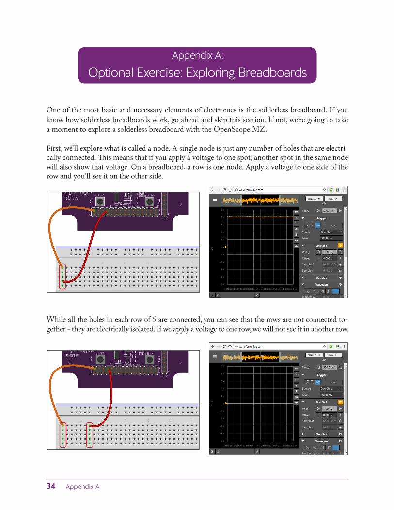
While all the holes in each row of 5 are connected, you can see that the rows are not connected to-gether - they are electrically isolated. If we apply a voltage to one row, we will not see it in another row.

Appendix A:

Optional Exercise: Exploring Breadboards

Appendix A 35

While the main breadboard surface has its nodes connected by rows, the power rails are connected by columns. Apply power to either the blue column or red column and you’ll see holes in that same column have that voltage.

You may have already figured this out since they are not physically connected, but the two power rails on either side of the main breadboard are also electrically isolated.

36 Appendix B

Appendix B:

Resistor Color Code Chart

Examples:

You can also use our app! https://reference.digilentinc.com/tools

Appendix C 37

Appendix C:

How to Read Capacitors

Ceramic Capacitor Electrolytic Capacitor

Another handy resource: http://www.electronics-tutorials.ws/capacitor/cap_3.html

The LEDs on the OpenScope MZ are used to indicate the current status of the OpenScope’s hardware as follows:

• Blue Off: Device is booting and not ready to use.• Blue Flashing: Device is booted and ready to use but Wi-Fi is not connected.• Blue Solid: Device is booted and ready to use and Wi-Fi is connected.• Red Solid - Calibration or acquisition in progress.• All user LEDs Solid - An error has occurred. Reboot the OpenScope MZ.

When connected to a Wi-Fi network, the 3 user LEDs display the last octet of the OpenScope MZ’s IP address by blinking the number of times corresponding to that digit of the last octet in decimal. For example, an OpenScope MZ with an IP address ending in ‘123’ would blink LD1 once, LD2 twice, and LD3 three times.

38 Appendix D

Appendix D:

Troubleshooting

Note: Firmware versions prior to 1.2.0 will not exhibit this LED behavior.

192.168.1.123

You may have noticed (and thought it odd) that throughout this workbook we didn’t just tell you to use the black ground wires. That is because the OpenScope MZ was designed to maximize signal integrity.

In this workbook, we only used the analog inputs of the OpenScope MZ; however, the OpenScope MZ also has digital input channels. If you were to use both the digital channels and the analog channels and used a single black ground wire, you would see noise from the digital channels show up on the analog channels. This is because they share a ground plane within the PCB.

That could be pretty misleading as you take your measurements, so we added two analog grounds. These are the blue wire with the white stripe and the orange wire with the white stripe that we used in the exercises.

As a rule of thumb: if you are using the analog channels, use the analog grounds. If you are using the digital channels, use the black digital ground.

Appendix E 39

Appendix E:

A Note on Grounding

40 Appendix F

Appendix F:

Helpful Links

Real Analog Course Material:https://reference.digilentinc.com/learn/courses/real-analog/start

Capacitor Tutorial:http://www.electronics-tutorials.ws/capacitor/cap_3.html

Resistor Calculator Application:https://reference.digilentinc.com/tools/

Digilent Documentation Wiki:reference.digilentinc.com

Digilent Github:https://github.com/digilent

OpenScope Resource Center:https://reference.digilentinc.com/reference/instrumentation/openscope-mz/start

For any additional questions post on our forum:

forum.digilentinc.com

Learning Edition WorkbookThe OpenScope MZ is an all-in-one WiFi enabled benchtop instrumentation tool. When combined with the software Waveforms Live, the OpenScope MZ turns your computer into an oscilloscope, waveform generator, power supply, simple logic analyzer, basic spectrum analyzer, and a data logger. With this tool, you can make the invisible visible, and you’ll be able to view signals right on your computer’s screen, giving you a clear picture of what is going on in your circuits! This workbook was created to introduce you to the OpenScope MZ, to measuring circuits, and provide you with helpful resources for learning more. We hope this is a jumping o point for your journey with instrumentation!

With this workbook, you should be able to:

• Successfully set up your OpenScope MZ • Take your first measurement • Get familiar with your Analog Parts Kit • Get an introduction to Ohm’s Law • Learn a little bit about power • View an RC circuit response • Explore triggering • View a frequency response • Learn about fast Fourier transforms • Get an intro to operational amplifiers • Learn how and where to get additional resources

Documents

Learning Edition Workbook - reference.digilentinc.com · Learning Edition Workbook Kaitlyn Franz, ... This workbook is designed to help you get started with electronics instrumentation