Learning Curves and Changing Product Attributes: the Case of Wind Turbines

Louis Coulomb and Karsten Neuhoff

February 2006

CWPE 0618 and EPRG 0601

These working papers present preliminary research findings, and you are advised to cite with caution unless you first contact the

author regarding possible amendments.

Learning curves and changing product attributes: the case of wind turbines

December 2005

Louis Coulomb and Karsten Neuhoff1

Abstract:

The heuristic concept of learning curves describes cost reductions as a function of cumulative production. A study of the Liberty shipbuilders suggested that product quality and production scale are other relevant factors that affect costs. Significant changes of attributes of a technology must be corrected when assessing the impact of learning-by-doing. We use an engineering-based model to capture the cost changes of wind turbines that can be attributed to changes in turbine size. We estimate the learning curve and turbine size parameters using more than 1500 price points from 1991 to 2003. The fit between model and empirical data confirms the concept.

1. Introduction The concept of learning curves is based on the empirical observation that costs of a technology fall by a constant proportion with every doubling of cumulative production. The concept was not derived from fundamental principles, but describes a phenomenon that was first identified in aeroplane construction by Wright (1936). The concept implies that expensive new technologies might become cost competitive with conventional technologies once increased application of the technology has provided sufficient learning and hence reduced the cost. This is one of the drivers in many government support programmes for renewable energy technologies. Learning curves are also an integral part of energy sector and macro-economic models that aim to understand the costs of adapting our economies to low carbon futures. 1 Both Faculty of Economics, University of Cambridge. Contact: Karsten.neuhoff@econ.cam.ac.uk. We are grateful for financial support provided by the Carbon Trust and by UK research council under the TSEC programme. We would also like to thank Dr. Martin Junginger (University of Utrecht) for providing us with the bulk of our price data, Michiel Zaaier (TU Delft) for his helpful comments on turbine scaling properties, and Richard Spencer (World Bank) for providing us with our initial data set.

1

Many studies have used the concept of learning curves to assess cost evolutions of, for instance, coal-fired power plants (Joskow and Rose, 1985), ethanol production (Goldemberg, 1996), PV modules (Watanabe, 1999) and wind turbines. Within the latter sector, studies have not only focused on different geographical systems, from global experience curves (Junginger et al., 2005) to country-specific ones (Neij et al., 2003); but also on different system levels, from the price of electricity (Ibenholt, 2002; IEA, 2000) to the price of wind farms ( Klaasen et al, 2003; Junginer et al., 2005), to the price of wind turbines (Durstewitz and Hoppe-Kilpper, 1999; Neij et al, 2003). A good overview of wind energy learning curves can be found in Junginger et al. (2005).

One of the classical examples of learning-by-doing can be found in the WWII Liberty shipbuilders data. Thompson’s (2001) careful analysis of the data revealed the need to compare homogeneous products in learning curve analysis; a significant portion of the ship building productivity increases could not be attributed solely to learning-by-doing, as had previously been assumed, but also to reduced product quality, measured in terms of fracture rates, and changes in available capital. Representing these changes improves the fit with empirical data and the ability to anticipate future cost trends.

Thompson’s analysis illustrates the benefit of careful study of individual technologies. A technology can have multiple attributes; for instance, quality increases availability and reduces maintenance costs; durability reduces the risk of early decommissioning; and innovative technology, such as the new direct-drive (gearless) systems, although generally more expensive for the same power rating, reduces subsequent maintenance costs. Changes in these attributes over time can impact the production costs of turbines, for example, if more expensive materials are used. If changes in these attributes are not reflected in the estimation of a learning-by-doing rate, then results can be biased In the case of wind turbines, the average turbine size has increased from ~27m rotor diameter in 1990 to ~65m rotor diameter in 2003 (based on IEA, 2003). To ensure that the blades do not touch the ground, a higher tower also accompanies the bigger rotor diameter. Increased wind speed at higher tower heights, due to wind shear, increases the potential energy capture of a turbine. When we corrected turbine price data for this effect, the fit with observed price data was not improved proportionally because turbine size has non-linear effects on both turbine costs and energy captured.

For this reason, we propose to use an engineering-based model to correct for the cost changes of wind turbines that can be attributed to the changing turbine size. We break down the turbine into components, with different scaling properties relative to turbine size; for example, the costs of generators varies with the square of the rotor diameter, while the mass of the nacelle, and hence the cost, increases with the cube of the rotor diameter. Weighting the different components with their cost contribution to the turbine gives a non-linear relationship between turbine size and turbine costs, with reference size and reference price as two free parameters. Finally, combining the engineering model with the learning-by-doing

2

function adds the learning curve parameter to the equation. We estimate these three parameters using more than 1500 German list prices, power ratings, tower height and the global installed capacity of wind turbines for each of these years. Using the combined learning-by-doing and engineering model we obtain a good fit for all of the list price data. This confirms the concept of learning curves for energy technologies, but also the necessity of correcting for significant changes in turbine size.

With our approach, we obtain a learning rate of about 12% using the German price data and global cumulative installed capacity for the period 1991-2003. Existing studies that examine learning curves for ex works turbine prices (ISET, 2005; Neij et al, 2003) calculate much lower learning rates (5-6%) based on yearly output-weighted average prices, using cumulative installed capacity for Germany (rather than the global capacity) to explain the price reductions. We consider international interaction in the observation period to be sufficiently active to justify the use of global installed capacity as an explanatory variable for cost reductions also within Germany.

Initially we were puzzled as to why it did not suffice to simply correct turbine prices for the difference in energy delivered at different sizes (based on the power rating) to obtain a good match with list prices. We think that size of wind turbines is a significant attribute that influences the value of a turbine without being properly reflected in the turbine price. There are two main reasons for this.

Firstly, the compound product “wind energy” consists not only of the wind turbines, but also of the complementary aspects of project development, grid connection, system balancing costs etc., which generally decrease (per kW) with increasing turbine size. Investors will therefore not necessarily choose the cheapest turbine but the turbine best suited for surrounding energy system, which includes the incentives created by renewable energy support mechanisms. Recent academic work has addressed some of these concerns by expanding the learning system being considered, calculating learning curves based on the price of wind farms (Klaasen et al, 2002; Junginer et al., 2005) or the tariff price of electricity produced (Ibenholt, 2002; IEA, 2000).

Secondly, the range of turbines that is available in the market has increased over time. Turbine producers have gained experience and gradually increased turbine size. In the early 1990s, this created economies of scale, but in recent years, our analysis suggests dis-economies of scale for wind turbines. Part of the cost reductions from learning-by-doing did not reduce the turbine price but simply allowed for the bigger turbine sizes. Please note that the existence of dis-economies of scale at the turbine level does not imply that the size of current turbines is too large, because such a statement requires an assessment that includes all the costs and benefits of integrating the turbine into the energy system.

Of these two points, only the second will be addressed in this paper, which deals exclusively with scale at the turbine level. We make the simplifying assumption that the production scale has not changed significantly over the last two decades as the continuous

3

increase in turbine size has prevented a shift towards mass production. A few studies have sought to distinguish production-scale effects from learning-effects in various technologies, ranging from PV and wind turbines (Isoard and Soria, 2001), and paper mills (Lundmark, 2003).

The paper is set out as follows: section 2 presents the theory of our combined engineering-learning model. Section 3 details the data used for the analysis; results are presented in section 4 and interpreted in section 5. Section 6 concludes. 2 The model

We first introduce the economic concept of the learning curve using the following

notation: K is the cumulative capacity installed of a technology and c(.) the cost of one

standardised unit of the technology, c0 the intercept for the cost of the initial unit and b the

slope of the learning curve (on a log-log scale): bKcKc 0)( = . (1)

The slope of the learning-by-doing function can be expressed as progress ratio, P: bP 2= (2)

or as the learning rate, L: bL 21−= (3)

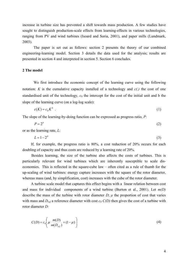
If, for example, the progress ratio is 80%, a cost reduction of 20% occurs for each doubling of capacity and thus costs are reduced by a learning rate of 20%. Besides learning, the size of the turbine also affects the costs of turbines. This is particularly relevant for wind turbines which are inherently susceptible to scale dis-economies. This is reflected in the square-cube law – often cited as a rule of thumb for the up-scaling of wind turbines: energy capture increases with the square of the rotor diameter, whereas mass (and, by simplification, cost) increases with the cube of the rotor diameter. A turbine scale model that captures this effect begins with a linear relation between cost and mass for individual components of a wind turbine (Burton et al., 2001). Let m(D) describe the mass of the turbine with rotor diameter D; μ the proportion of cost that varies with mass and Dref a reference diameter with cost c0 C(D) then gives the cost of a turbine with rotor diameter D:

⎟⎟⎠

⎞⎜⎜⎝

⎛−+= )1(

)()()( 0 μμ

refDmDmcDC (4)

4

The mass function, m(D), is not uniform for the various components of a wind turbine. Following Burton et al. (2001), we assume that the weight of the generator scales with the energy and thus quadratically with D. Assuming a constant tip speed, the rotational speed of the blades decreases proportionally with D, and therefore the torque at the nacelle increases with the cube of D and thus the mass of the rotor and the stress-bearing components of the nacelle also scale with the cube of D. The change of the turbine cost with size can now be described as the sum of the changes to the components. For this purpose, we define xi as the fraction of turbine mass which scales with the rotor diameter with exponent i. As we aim to compare turbines of different sizes, we “normalise” the turbine costs by dividing through captured energy, which scales with the square of D (given in the denominator):

2

1

2

2

3

3

0

1

)(

⎟⎟⎠

⎞⎜⎜⎝

⎛

−+⎟⎟⎠

⎞⎜⎜⎝

⎛+⎟

⎟⎠

⎞⎜⎜⎝

⎛+⎟

⎟⎠

⎞⎜⎜⎝

⎛

=

ref

refrefref

DD

DDx

DDx

DDx

cDc

μμμμ (5)

While there is some variation in the cost share of different components from turbine to turbine, there is no significant shift in the cost structure of turbines with increasing size of the turbine (Hau, 2000); thus, a constant component cost structure can reasonably be assumed for all turbine sizes (see Table 1.). We can now combine the learning curve function (1) with the engineering-based scale model (5):

b

ref

refrefrefK

DD

DDx

DDx

DDx

cDc 2

1

2

2

3

3

0

)1(

)(

⎟⎟⎠

⎞⎜⎜⎝

⎛

⎥⎥

⎦

⎤

⎢⎢

⎣

⎡−+⎟

⎟⎠

⎞⎜⎜⎝

⎛+⎟

⎟⎠

⎞⎜⎜⎝

⎛+⎟

⎟⎠

⎞⎜⎜⎝

⎛

=

μμμμ

(6)

The tower height increases proportionally with the rotor diameter, and wind speed increases with hub height due to wind shear. The typical exponential approximation for the wind speed profile at hub height H, relative to a reference wind speed Vref , at reference height Href is:

α

⎟⎟⎠

⎞⎜⎜⎝

⎛=

refref H

HVHV )( (7)

5

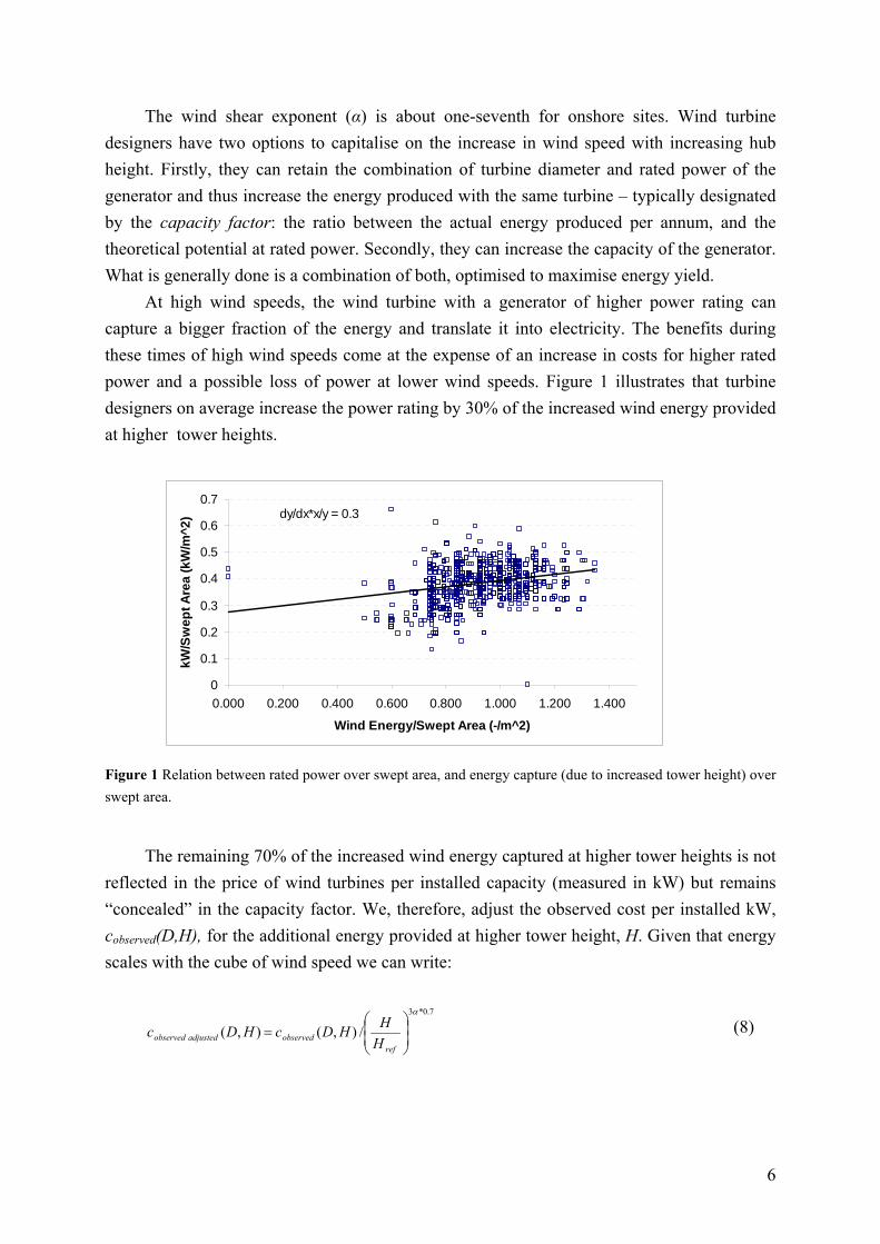
The wind shear exponent (α) is about one-seventh for onshore sites. Wind turbine designers have two options to capitalise on the increase in wind speed with increasing hub height. Firstly, they can retain the combination of turbine diameter and rated power of the generator and thus increase the energy produced with the same turbine – typically designated by the capacity factor: the ratio between the actual energy produced per annum, and the theoretical potential at rated power. Secondly, they can increase the capacity of the generator. What is generally done is a combination of both, optimised to maximise energy yield. At high wind speeds, the wind turbine with a generator of higher power rating can capture a bigger fraction of the energy and translate it into electricity. The benefits during these times of high wind speeds come at the expense of an increase in costs for higher rated power and a possible loss of power at lower wind speeds. Figure 1 illustrates that turbine designers on average increase the power rating by 30% of the increased wind energy provided at higher tower heights.

0

0.1

0.2

0.3

0.4

0.5

0.6

0.7

0.000 0.200 0.400 0.600 0.800 1.000 1.200 1.400

Wind Energy/Swept Area (-/m^2)

kW/S

wep

t Are

a (k

W/m

^2) dy/dx*x/y = 0.3

Figure 1 Relation between rated power over swept area, and energy capture (due to increased tower height) over swept area.

The remaining 70% of the increased wind energy captured at higher tower heights is not reflected in the price of wind turbines per installed capacity (measured in kW) but remains “concealed” in the capacity factor. We, therefore, adjust the observed cost per installed kW, cobserved(D,H), for the additional energy provided at higher tower height, H. Given that energy scales with the cube of wind speed we can write:

7.0*3

/),(),(α

⎟⎟⎠

⎞⎜⎜⎝

⎛=

refobservedadjustedobserved H

HHDcHDc (8)

6

The remaining 30% of increased wind energy captured at higher tower heights is used to increase the power rating by installing bigger generators per area swept by the rotor. We can now adjust (6) accordingly (see the denominator):

b

refref

refrefrefK

HH

DD

DDx

DDx

DDx

cHDc 3.0*32

1

2

2

3

3

0

)1(

),( α

μμμμ

⎟⎟⎠

⎞⎜⎜⎝

⎛⎟⎟⎠

⎞⎜⎜⎝

⎛

⎥⎥

⎦

⎤

⎢⎢

⎣

⎡−+⎟

⎟⎠

⎞⎜⎜⎝

⎛+⎟

⎟⎠

⎞⎜⎜⎝

⎛+⎟

⎟⎠

⎞⎜⎜⎝

⎛

= (9)

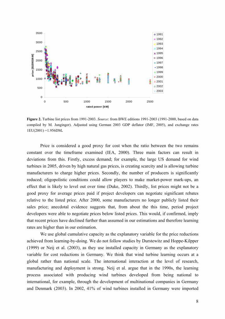
Equations (7) and (9) form the basis of the regression analysis we use to determine the simultaneous learning and turbine scale effects. The 70% of the additional energy captured at higher hub heights is “concealed” in the capacity factor and thus not reflected in the power rating or turbine price. Learning curve analysis based on installed capacity (the sum of turbine rated power; kW) as the energy benchmark - but in which the rated power is not adjusted to account for this effect - omit an important contribution. Other studies avoid this problem by using kWh as the energy benchmark; here, a reference wind site is selected, and the annual theoretical energy production of all turbines that constitute the installed capacity is determined. The problem with the latter approach is that, while it more accurately reflects the progress in energy production, the energy benchmark, kWh, makes comparison with other energy technologies difficult. For this reason in particular, we selected a method in which the kW benchmark is retained, and the additional energy capture is at least partly reflected. 3 Data Our principal data source is list prices from the catalogues of the German Wind Energy association for the period 1991-2003 (BWE). The data set also provides the rotor diameter and tower height for the over 1500 listed turbines (see Figure 2). We exclude all turbines with a rotor diameter of less than 10m: this represents less than 10 data points. These very small turbines have somewhat different engineering characteristics and control characteristics and would thus require additional parameters for their representation. In a robustness test, we included these data points and obtained higher learning rates and a lower reference rotor diameter. Given the sensitivity of the results to these few points and the fact that the bulk of our data lies at approximately 20m rotor diameter and above, we deem it justifiable to exclude these points.

7

0

500

1000

1500

2000

2500

3000

3500

0 500 1000 1500 2000 2500

rated power [kW]

pric

e [E

U200

3/kW

]1991

19921993

19941995

19961997

19981999

20002001

20022003

Figure 2. Turbine list prices from 1991-2003. Source: from BWE editions 1991-2003 (1991-2000, based on data compiled by M. Junginger). Adjusted using German 2003 GDP deflator (IMF, 2005), and exchange rates 1EU(2001) =1.956DM.

Price is considered a good proxy for cost when the ratio between the two remains

constant over the timeframe examined (IEA, 2000). Three main factors can result in deviations from this. Firstly, excess demand; for example, the large US demand for wind turbines in 2005, driven by high natural gas prices, is creating scarcity and is allowing turbine manufacturers to charge higher prices. Secondly, the number of producers is significantly reduced; oligopolistic conditions could allow players to make market-power mark-ups, an effect that is likely to level out over time (Duke, 2002). Thirdly, list prices might not be a good proxy for average prices paid if project developers can negotiate significant rebates relative to the listed price. After 2000, some manufacturers no longer publicly listed their sales price; anecdotal evidence suggests that, from about the this time, period project developers were able to negotiate prices below listed prices. This would, if confirmed, imply that recent prices have declined further than assumed in our estimations and therefore learning rates are higher than in our estimation.

We use global cumulative capacity as the explanatory variable for the price reductions achieved from learning-by-doing. We do not follow studies by Durstewitz and Hoppe-Kilpper (1999) or Neij et al. (2003), as they use installed capacity in Germany as the explanatory variable for cost reductions in Germany. We think that wind turbine learning occurs at a global rather than national scale. The international interaction at the level of research, manufacturing and deployment is strong. Neij et al. argue that in the 1990s, the learning process associated with producing wind turbines developed from being national to international, for example, through the development of multinational companies in Germany and Denmark (2003). In 2002, 41% of wind turbines installed in Germany were imported

8

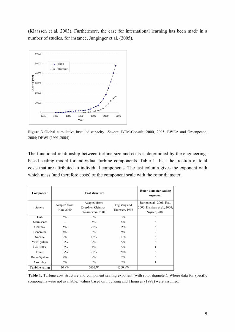
(Klaassen et al, 2003). Furthermore, the case for international learning has been made in a number of studies, for instance, Junginger et al. (2005).

0

10000

20000

30000

40000

50000

60000

1975 1980 1985 1990 1995 2000 2005

Year

Capa

city

(MW

)

global

Germany

Figure 3 Global cumulative installed capacity Source: BTM-Consult, 2000, 2005; EWEA and Greenpeace, 2004; DEWI (1991-2004)

The functional relationship between turbine size and costs is determined by the engineering-based scaling model for individual turbine components. Table 1 lists the fraction of total costs that are attributed to individual components. The last column gives the exponent with which mass (and therefore costs) of the component scale with the rotor diameter.

Component Cost structure Rotor diameter scaling exponent

Source Adapted from:

Hau, 2000

Adapted from: Dresdner Kleinwort Wasserstein, 2001

Fuglsang and Thomsen, 1998

Burton et al., 2001; Hau, 2000; Harrison et al., 2000;

Nijssen, 2000 Hub 5% 3% 3% 3

Main shaft - 5% 5% 3 Gearbox 5% 22% 15% 3

Generator 6% 8% 9% 2 Nacelle 7% 12% 13% 3

Yaw System 12% 2% 5% 3 Controller 13% 4% 5% 1

Tower 17% 20% 20% 3 Brake System 4% 2% 2% 3

Assembly 5% 3% 2% 1

Turbine rating 30 kW 600 kW 1500 kW

Table 1. Turbine cost structure and component scaling exponent (with rotor diameter). Where data for specific components were not available, values based on Fuglsang and Thomsen (1998) were assumed.

9

In our analysis, we assume a cubic relationship between costs of the tower and rotor diameter. Nijsen (2000) argues that tower design is governed principally by fatigue; the cubic relation assumed is a conservative estimate based on the maximum moment at the tower base. We also include assembly and erection costs in the cost model, as they are included in the quoted prices; we assume these scale linearly with rotor diameter.

Table 2 gives the remaining assumptions for the base case of the regression analysis. value Comments μ - Proportion of cost mass dependent

90% Source: Burton et al., 2001

Shear exponent 1/7 Typical for onshore terrain

Minimum rotor diameter 10m The inclusion of these data bias the results towards higher learning rates

Href 50m this value is arbitrary and only affects c0 Quality adjustment ratio 70% See section 2 Cost structure See Table 1 Source: Fuglsang and Thomsen, 1998

Table 2 Base case input parameters

10

0

1000

2000

3000

4000

5000

6000

0 10 20 30 40 50 60 70 80

Rotor diameter (m)

Figure 4. Scale and learning components for the base case

Figure 5. Results of fits for datasets corresponding to specific years

0

1000

2000

3000

4000

5000

6000

0 10 20 30 40 50 60 70 80

Rotor diameter (m)

EU2

003/

kW

1991

0

1000

2000

3000

4000

5000

6000

0 10 20 30 40 50 60 70 80Rotor diameter (m)

EU20

03/k

W

1994

0

1000

2000

3000

4000

5000

6000

0 10 20 30 40 50 60 70 80

Rotor diameter (m)

EU20

03/k

W

1997

0

1000

2000

3000

4000

5000

6000

0 10 20 30 40 50 60 70 80

Rotor diameter (m)

EU

2003

/kW

2000

0

1000

2000

3000

4000

5000

6000

0 10 20 30 40 50 60 70 80

Rotor diameter (m)

EU2

003/

kW

2003

EU

2003

/kW

List PricesEstimator

Only scale

0

1000

2000

3000

4000

5000

6000

0 10 20 30 40 50 60 70 80Rotor diameter (m)

EU

2003

/kW

List Prices

Only Learning

Only learning

11

4. Model analysis We estimate the learning rate and reference diameter for which our model (9) best fits the data, using a non-linear least square estimation. Table 3 gives the estimated reference diameter and learning rates. In the first row, all observation points receive equal weighting. However, both the early and late years of the observation period were characterised by fewer observation points per year. In the second row, observation points are weighted in such a way that the aggregate observations for each year receive the same weighting.

Estimation c0Standard deviation

DrefStandard deviation

b Standard deviation

Log likelihood

Equal weight per observation

4018 570 52.4 1.1 -0.158 0.016 -11137

Equal weight per year

5744 860 50.3 1.1 -0.197 0.017 -11229

Table 3. Regression results for the base case, based on different data weighting approaches

Please note that the log likelihood cannot be compared between these cases, as the

different weighting of observations effectively implies an estimation of a different data set. Figure 4 illustrates that it is difficult to fit all the observed data with a model for only

turbine scale or only learning-by-doing. Figure 5 shows data fits for specific years from 1991 to 2003. Table 4 translates the results from Table 3 into learning rates and a typical power rating. The optimal power rating is based on the rotor diameter for which for the model yields the lowest costs per turbine. Grid connection and planning contribute additional costs, which are less dependent on turbine size. If we assume, for instance, that such costs are € 200,000 per turbine, the optimal turbine size increases (see Table 4).

Estimation learning rate std Optimal power

rating turbine

Optimal power rating turbine +

€200,000 fixed costs

Equal weight per observation

10.4% 1% 400-500 kW 900-1000 kW

Equal weight per year 12.7% 1% 400-500 kW 900-1000 kW

Table 4 Learning rates and optimal power rating

A series of tests have been performed in order to determine the robustness of the

results. They are related to the base case with equal weighting on different years (which implies different weighting of observations within each year).

The first robustness test, Table 5, considers the parameter μ, which represents the proportion of the cost that varies with mass, and hence rotor diameter. Engineering literature suggests that between 75% and 95% of mass is turbine scale dependent (Burton et al, 2001;

12

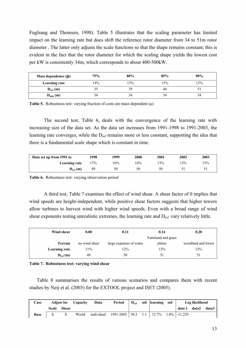
Fuglsang and Thomsen, 1998). Table 5 illustrates that the scaling parameter has limited impact on the learning rate but does shift the reference rotor diameter from 34 to 51m rotor diameter . The latter only adjusts the scale functions so that the shape remains constant; this is evident in the fact that the rotor diameter for which the scaling shape yields the lowest cost per kW is consistently 34m, which corresponds to about 400-500kW.

Mass dependence (μ) 75% 80% 85% 90%

Learning rate 14% 13% 13% 13%

Dref (m) 35 39 44 51

Dmin (m) 34 34 34 34

Table 5. Robustness test: varying fraction of costs are mass dependent (μ)

The second test, Table 6, deals with the convergence of the learning rate with

increasing size of the data set. As the data set increases from 1991-1998 to 1991-2003, the learning rate converges, while the Dref remains more or less constant, supporting the idea that there is a fundamental scale shape which is constant in time.

Data set up from 1991 to 1998 1999 2000 2001 2002 2003 Learning rate 17% 16% 14% 13% 13% 13%

Dref (m) 49 50 50 50 51 51

Table 6. Robustness test: varying observation period

A third test, Table 7 examines the effect of wind shear. A shear factor of 0 implies that

wind speeds are height-independent, while positive shear factors suggests that higher towers allow turbines to harvest wind with higher wind speeds. Even with a broad range of wind shear exponents testing unrealistic extremes, the learning rate and Dref vary relatively little.

Wind shear 0.00 0.11 0.14 0.28

Terrain no wind shear large expanses of waterFarmland and grass

plains woodland and forest Learning rate 11% 12% 13% 13%

Dref (m) 49 50 51 51

Table 7. Robustness test: varying wind shear

Table 8 summarises the results of various scenarios and compares them with recent

studies by Neij et al. (2003) for the EXTOOL project and ISET (2005).

Case Adjust for Capacity Data Period Dref std learning std Log likelihood Scale Shear data 1 data2 data3

Base X X World individual 1991-2003 50.3 1.1 12.7% 1.0% -11,229

13

1 X World individual 1991-2003 49.1 20.9 10.9% 0.9% -11,123 2 X World individual 1991-2003 17.2% 0.5% -11,851 3 World individual 1991-2003 11.0% 1.1% -11,593 4 Germany individual 1991-2003 7.2% 0.6% -11,534

ISET Germany annual av. 1990-2003 5.0% EXTOOL Germany annual av. 1990-2000 6.0% EXTOOL Germany annual av. 1987-2000 4.0%

Table 8 Comparison of different scenario runs with results from recent studies. Note: Extool values are for rated power ≥ 55kW

First, we note a decrease of the log-likelihood value that results from excluding scale

effect as the explanatory variable: in the model with wind shear 622 (base case and case 2), without wind shear 470 (cases 1 and 3). Both differences exceed single digits and therefore the model is significantly poorer in explaining the observations than if these factors were not included. We cannot use the same approach to compare a model with and without shear effect, as the corresponding representations are not nested.

It is interesting to observe that all the models that include wind shear produce significantly higher learning rates. The difference can be explained as follows. Assume a model does not capture the wind shear: it only compares turbines based on their rated power. The model ignores the fact that between 1991 and 2003, tower height has increased significantly, thus exposing wind turbines to higher wind speed and increasing their load factor by approximately 30%.2 In the same period, the global installed wind capacity doubled 4.2 times. This would suggest that, with every doubling of global wind capacity, the load factor increased by 6%. This can also be interpreted as showing that, with every doubling of global installed capacity, the effective costs of wind turbines decreased by an additional 6%. This number roughly corresponds to the impact, which the shear factor has when no scale effect is modelled (case 2 vs. case 3). If the scale effect is modelled, then exclusion of the shear factor has less impact on the learning rate but reduces the fit of the scaling function, as illustrated by the significantly larger standard deviation calculated for Dref.

Both Extool and ISET used the cumulative installed capacity in Germany to explain the evolution of German list prices. Between 1991 and 2003, installed capacity in Germany doubled 7.2 times, as it increased from 0.1GW to 14.6GW. In the same period, global installed capacity only doubled 4.2 times as it increased from 2.2GW to 40.3GW. Thus the learning that can be attributed to any one doubling is smaller if we use the German installed capacity as an explanatory variable, as illustrated by comparison of cases 3 and 4. Once again, changing the input data means that a comparison of the log-likelihood values to determine

2 If we assume rotor diameter corresponds to turbine height and 67% of additional wind energy results in additional wind output (see section 2), then the increase of rotor diameter from 27m to 65m results in an increase of 30% of the load factor. i.e. (1-(65/27)^α*67%)

14

which model fits better is not possible. As discussed above, we decided to use global installed capacity as the input variable for our analysis because of the international, scientific, industrial and market interaction during the observation period. Using the German input data and ignoring scale and shear effects, we observe similar learning rates to those of ISET and EXTOOL (case 4). We note, however, that both these studies first calculate an annual average turbine price by weighting the turbine list prices with the installation volume of each turbine type. The experience curve is then fitted to the annual average prices reducing the regression data set to the numbers examined, i.e. 10-15 values. Much information contained in the diverse set of prices within each year is aggregated, and thus lost, in their study. 5 Conclusions.

We test the heuristic concept of learning by doing with the example of wind turbines. Following the careful analysis of Thompson (2001), we ensure that significant changes in attributes of the turbines are represented in the model. As the size of wind turbines has increased during the observation period, we use an engineering-based model to represent the cost changes as a function of turbine size. In combination with the learning-by-doing model, we obtain an excellent fit with 1500 price observation points for the period 1991-2003. This extends existing literature, which has used output-weighted average annual wind turbine prices and has ignored much of the structure present in the data.

Our estimation shows that with every doubling of global installed capacity, costs of wind turbines per installed capacity have fallen by 10.9%. However, this estimation ignores the fact that bigger turbines are exposed to higher wind speeds at higher tower heights and therefore produce more energy per installed capacity. Allowing the model to correct for this effect, we estimate that costs for wind turbines have fallen by 12.7% with every doubling of installed capacity.

The model also allows us to estimate economies of scale at the unit turbine level. Turbine costs fall with size below approximately 400-500 kW and increase for bigger turbines. Additional costs related to project development, civil works, grid connection etc., only exhibit limited size dependence, and thus increase the optimal size of turbines as part of the overall system. The optimal turbine size from the perspective of a project developer is therefore bigger, as confirmed by the large-scale application of 2MW turbines.

We observe that learning-by-doing in wind turbines has allowed the simultaneous processes of cost reductions and increases in turbine size. This creates two non-convexities that can inhibit competitive markets from developing a new technology. Firstly, the new technology would initially be more expensive because of less historic learning-by-doing and would thus capture a smaller market share. Secondly, if the new technology requires manufacturers to experiment with small turbines and then gradually increase their size, then the economics of scale imply that early turbines are more expensive than later turbines.

15

This study does not propose an optimal turbine size. As has been discussed, such a statement would necessitate the examination of the larger system that describes the cost of producing electricity from wind, which includes not only wind turbines, but the costs of project development, grid connection, foundation works, etc. However, it is conceivable that turbines will converge on an optimal turbine size. Subsequently, we would no longer observe the current dis-economies of scale at the turbine level, resulting in faster cost reductions. Furthermore, the demand for increasing turbine size implied that engineers had to satisfy two objectives: increasing turbine size and reducing costs. At a constant turbine size, more focus can be attributed to cost improvements.

In our study, we do not assess economies of scale in the production of wind turbines, nor changes of quality, durability and availability of wind turbines during the observation period. If these have resulted in significant changes, then additional corrections are required to obtain an unbiased estimate of the learning-by-doing rate. Correcting for turbine size already significantly improves the fit with observed data and further confirms that the heuristic concept of learning by doing provides a good description of the cost evolution of wind turbines. References Boston Consulting Group (1968). Perspectives on experience. Boston Consulting Inc. BTM-Consult ApS. (2004). International Wind Energy Development - World Market Update 2003. BTM-Consult ApS. (2005). Press Release – International Wind Energy Development, World Market Update 2004. 31 March 2005. Burton, T., Sharpe, D. Jenkins and N., Bossanyi, E. (2001). Handbook of Wind Energy. John Wiley and Sons, Ltd. Chichester, UK. BWE, Editions (1991-2003). Windenergie. Osnabrück, Germany, Bundesverband Windenergie. DEWI Online Magazine (1991-2004). Deutsches Windenergie Institut. http://www.dewi.de/dewi_neu/deutsch/themen/magazin/ Dresdner Kleinwort Wasserstein (2001). Power generation in the 21st century, part II: Renewables gaining ground. Duke, R. (2002). Clean energy technology buydowns: Economic theory, analytic tools, and the photovoltaics case. Ph.D. Dissertation, Princeton.

16

Durstewitz, M. and Hoppe-Kilpper, M. (1999). Wind Energy Experience Curve for the German “250 MW Wind-program” . IEA International Workshop on Experience Curves for Policy Making – The Case of Energy Technologies, Stuttgart, Germany. EWEA (2004). Wind Energy – The Facts. European Wind Energy Association, Brussels Belgium. EWEA and Greenpeace (2004). Wind Force 12; a blueprint to achieve 12% of the world’s electricity from wind power by the year 2020. European Wind Energy Association, Brussels Belgium. Fuglsang, P. and Thomsen K. (1998). Cost Optimization of Wind Turbines for Large Scale Offshore Wind Farms. Risoe National Laboratory Report No. R-1000. Risoe National Laboratory, Roskilde Denmark. Goldemberg, J. (1996). The evolution of ethanol costs in Brazil. Energy Policy, 24 (12), 1127-1128. Harrison, R., Hau, E. and Snel, H. (2000). Large Wind Turbines; Design and Economics. John Wile & Sons, Ltd. Chichester. Hau, E. (2000). Windturbines; Fundamentals, Technologies, Application and Economics. Springer Verlag, Berlin. IEA (2000). Experience Curve for Energy Technology Policy. International Energy Agency. Paris, France, IEA (2003). Renewable for Power Generation; Status and Prospects. International Energy Agency. Paris, France, ISET, 2005. Institute für Solare Energieversorgungstechnik e.V. Downloaded from: http://reisi.iset.uni-kassel.de/wind/reisi_dw.html Ibenholt, K. (2002). Explaining Learning Curves for Wind Power. Energy Policy, 30, pp. 1181-1189. Isoard, S. and Soria, A. (2001). Technical change dynamics: evidence from the emerging renewable energy technologies. Energy Economics 23, 2001. 619-636. Joskow, P.L. and Rose, N.L. (1985). The effects of technological change, experience and environmental regulation on the construction cost of coal-burning generating units. Rand Journal of Economics, Vol. 16, No. 1, Spring 1985. Junginger, M., Faaij, A. and Turkenburg, W.C. (2005). Global Experience Curves for Wind Farms. Energy Policy, 33, pp. 133-150. Klaassen, G., Miketa, A., Larsen, K., and Sundqvist, T. (2003). Public R&D and Innovation: The Case of Wind Energy in Denmark, Germany and the United Kingdom. International Institute for Applied Systems Analysis. Laxenburg, Austria.

17

Lundmark, R., (2003). On the existence of learning effects in Swedish kraft paper mills. International Institute of Applied Systems Analysis. Laxenburg, Austria. Morthorst, P.E. (2005). Wind Power – Status and Perspectives. Risoe National Laboratory, Roskilde, Denmark. Neij, L., Dannemand, A.P., Durstewitz, M.,Hoppe-Kilpper, M. and Morthorst, P.E. (2003) Final Report of EXTOOL – Experience Curves: a tool for energy policy programmes assessment. Lund, Sweden. Nijssen (2000). Scaling rules relevant to the Lagewey 50/70 wind turbine: literature study. MSc Thesis report, TU Delft. Thompson, P. (2001). How much did the liberty shipbuilders learn? New evidence for an old case study. Journal of Political Economy, Vol. 29, No. 1, pp.103—137. Watanabe, C. (1999) Industrial dynamism and the creation of a "virtuous cycle" between R&D, market growth and price reduction: The case of PV in Japan, Proceedings of the IEA International Workshop at Stuttgart, Germany, 10-11 May, 1999 World Bank (2002) Statistical Analysis of Wind Farm Cost and Policy Regimes. Working Paper. Asia Alternative Energy Program. Wright, T.P., (1936). Factors Affecting the Cost of Aeroplanes. Journal of Aeronautical Sciences, 3 (4), pp.122-128.

18