Learning-by-Doing, Organizational Forgetting,

and Industry Dynamics∗

David Besanko† Ulrich Doraszelski‡ Yaroslav Kryukov§

Mark Satterthwaite¶

December 21, 2008

Abstract

Learning-by-doing and organizational forgetting have been shown to be importantin a variety of industrial settings. This paper provides a general model of dynamiccompetition that accounts for these economic fundamentals and shows how they shapeindustry structure and dynamics. Previously obtained results regarding the dominanceproperties of firms’ pricing behavior no longer hold in this more general setting. Weshow that forgetting does not simply negate learning. Rather, learning and forgettingare distinct economic forces. In particular, a model with learning and forgetting can giverise to aggressive pricing behavior, market dominance, and multiple equilibria, whereasa model with learning alone cannot.

∗We have greatly benefitted from the comments and suggestions of the Editor, Steve Berry, and twoanonymous referees. We are also indebted to Lanier Benkard, Luis Cabral, Jiawei Chen, Stefano Demichelis,Michaela Draganska, Ken Judd, Pedro Marin, Ariel Pakes, Michael Ryall, Karl Schmedders, Chris Shan-non, Kenneth Simons, Scott Stern, Mike Whinston, and Huseyin Yildirim as well as the participants ofvarious conferences. Guy Arie and Paul Grieco provided excellent research assistance. Besanko and Do-raszelski gratefully acknowledge financial support from the National Science Foundation under Grant No.0615615. Doraszelski further benefitted from the hospitality of the Hoover Institution during the academicyear 2006/07. Kryukov thanks the General Motors Center for Strategy in Management at Northwestern’sKellogg School of Management for support during this project. Satterthwaite acknowledges gratefully thatthis material is based upon work supported by the National Science Foundation under Grant No. 0121541.

†Kellogg School of Management, Northwestern University, Evanston, IL 60208, d-besanko@kellogg.northwestern.edu.

‡Department of Economics, Harvard University, Cambridge, MA 02138, doraszelski@harvard.edu.§Department of Economics, Northwestern University, Evanston, IL 60208, kryukov@northwestern.edu.¶Kellogg School of Management, Northwestern University, Evanston, IL 60208, m-

satterthwaite@kellogg.northwestern.edu.

1 Introduction

Empirical studies provide ample evidence that the marginal cost of production decreaseswith cumulative experience in a variety of industrial settings. This fall in marginal cost isknown as learning-by-doing. More recent empirical studies also suggest that organizationscan forget the know-how gained through learning-by-doing due to labor turnover, periodsof inactivity, and failure to institutionalize tacit knowledge.1 Organizational forgetting hasbeen largely ignored by the theoretical literature. This is problematic because Benkard(2004) shows that organizational forgetting is essential to explain the dynamics in themarket for wide-bodied airframes in the 1970s and 1980s.

In this paper we build on the computational Markov-perfect equilibrium framework ofEricson & Pakes (1995) to analyze how the economic fundamentals of learning-by-doing andorganizational forgetting interact to determine industry structure and dynamics.2 We addorganizational forgetting to Cabral & Riordan’s (1994) (C-R) seminal model of learning-by-doing.3 This seemingly small change has surprisingly large effects. Dynamic competitionwith learning and forgetting is akin to racing down an upward moving escalator. As longas a firm makes sales sufficiently frequently so that the gain in know-how from learningoutstrips the loss in know-how from forgetting, it moves down its learning curve and itsmarginal cost decreases. However, if sales slow down or come to a halt, perhaps becauseof its competitors’ aggressive pricing, then the firm slides back up its learning curve andits marginal cost increases. This cannot happen in the C-R model. Due to this qualitativedifference, organizational forgetting leads to a rich array of pricing behaviors and industrydynamics that the existing literature neither imagined nor explained.

It is often said that learning-by-doing promotes market dominance because it gives amore experienced firm the ability to profitably underprice its less experienced rival andtherefore shut out the competition in the long run. As Dasgupta & Stiglitz (1988) explain:

. . . firm-specific learning encourages the growth of industrial concentration.To be specific, one expects that strong learning possibilities, coupled with vigor-ous competition among rivals, ensures that history matters . . . in the sense that

1See Wright (1936)HIRS:52, DeJong (1957), Alchian (1963), Levy (1965), Kilbridge (1962), Hirschmann(1964), Preston & Keachie (1964), Baloff (1971), Dudley (1972), Zimmerman (1982), Lieberman (1984),Gruber (1992), Irwin & Klenow (1994), Jarmin (1994), Pisano (1994), Bohn (1995), Hatch & Mowery(1998), Thompson (2001), and Thornton & Thompson (2001) for empirical studies of learning-by-doing andArgote, Beckman & Epple (1990), Darr, Argote & Epple (1995), Benkard (2000), Shafer, Nembhard &Uzumeri (2001), and Thompson (2003) for organizational forgetting.

2Dynamic stochastic games and feedback strategies that map states into actions date back at least toShapley (1953). Maskin & Tirole (2001) provide the fundamental theory showing how many subgame perfectequilibria of these games can be represented consistently and robustly as Markov perfect equilibria.

3Prior to the infinite-horizon price-setting model of C-R, the literature had studied learning-by-doingusing finite-horizon quantity-setting models (Spence 1981, Fudenberg & Tirole 1983, Ghemawat & Spence1985, Ross 1986, Dasgupta & Stiglitz 1988, Cabral & Riordan 1997).

2

if a given firm enjoys some initial advantages over its rivals it can, by under-cutting them, capitalize on these advantages in such a way that the advantagesaccumulate over time, rendering rivals incapable of offering effective competitionin the long run . . . (p. 247)

However, if organizational forgetting “undoes” learning-by-doing, then forgetting may be aprocompetitive force and an antidote to market dominance through learning. Two reasonsfor suspecting this come to mind. First, to the extent that the leader has more to forgetthan the follower, forgetting should work to equalize differences between firms. Second,because forgetting makes improvements in competitive position from learning transitory, itshould make firms reluctant to invest in the acquisition of know-how through price cuts. Wereach the opposite conclusion: Organizational forgetting can make firms more aggressiverather than less aggressive. This aggressive pricing behavior, in turn, puts the industry ona path towards market dominance.

In the absence of organizational forgetting, the price that a firm sets reflects two goals.First, by winning a sale, the firm moves down its learning curve. This is the advantage-building motive. Second, the firm prevents its rival from moving down its learning curve.This is the advantage-defending motive. But in the presence of organizational forgettingbidirectional movements through the state space are possible, and this opens up new strate-gic possibilities for building and defending advantage. By winning a sale, a firm makes itselfless vulnerable to forgetting by creating a “buffer stock” of know-how. By winning and deny-ing its rival a buffer stock, the firm also makes its rival more vulnerable to forgetting. Be-cause organizational forgetting reinforces the advantage-building and advantage-defendingmotives in this way, it can create strong incentives to cut prices in order to win the sale.Organizational forgetting is thus a source of aggressive pricing behavior.

While the existing literature has mainly focused on the dominance properties of firms’pricing behaviors, we find that these properties are neither necessary nor sufficient for mar-ket dominance in our more general setting. We therefore go beyond the existing literatureand directly examine the industry dynamics that firms’ pricing behaviors imply. We findthat organizational forgetting is a source of—not an antidote to—market dominance. Ifforgetting is sufficiently weak, then asymmetries may arise but cannot persist. As in theC-R model, learning-by-doing operates as a ratchet: firms inexorably—if at different rates—move towards the bottom of their learning curves where cost parity obtains. If forgetting issufficiently strong, then asymmetries cannot arise in the first place because forgetting stiflesinvestment in learning altogether. But, for intermediate degrees of forgetting, asymmetriesarise and persist. Even extreme asymmetries akin to near-monopoly are possible. This isbecause, in the presence of organizational forgetting, the leader can use price cuts to delayor even stall the follower in moving down its learning curve.

3

Organizational forgetting is also a source of multiple equilibria. If the inflow of know-howinto the industry due to learning is substantially smaller than the outflow of know-how due toforgetting, then it is virtually impossible that both firms reach the bottom of their learningcurves. Conversely, if the inflow is substantially greater than the outflow, then it is virtuallyinevitable that they do reach the bottom. In both cases, the primitives of the model tiedown the equilibrium. This is no longer the case if the inflow roughly balances the outflow.If both firms believe that they cannot profitably coexist at the bottom of their learningcurves, then both cut their prices in the hope of acquiring a competitive advantage earlyon and maintaining it throughout. However, if both firms believe that they can profitablycoexist, then neither cuts its price, thereby ensuring that the anticipated symmetric industrystructure emerges. Consequently, in addition to the degree of forgetting, the equilibriumby itself is an important determinant of pricing behavior and industry dynamics.

Our finding of multiplicity is important for two reasons. First, to our knowledge, allapplications of Ericson & Pakes’s (1995) framework have found a single equilibrium. Pakes& McGuire (1994) (P-M) indeed held that “nonuniqueness does not seem to be a problem”(p. 570). It is therefore striking that we obtain up to nine equilibria for some parameteriza-tions. Second, we show that multiple equilibria in our model arise from firms’ expectationsregarding the value of continued play. Being able to pinpoint the driving force behind mul-tiple equilibria is a first step towards tackling the multiplicity problem that plagues theestimation of dynamic stochastic games and inhibits the use of counterfactuals in policyanalysis.4

In sum, learning-by-doing and organizational forgetting are distinct economic forces.Forgetting, in particular, does not simply negate learning. The unique role forgetting playscomes about because it makes bidirectional movements through the state space possible.Thus the interaction of learning and forgetting can give rise to aggressive pricing behavior,long-run market dominance of varying degrees, and multiple equilibria.

We emphasize that organizational forgetting is not unique in leading to long-run marketdominance. As we show in Section 8, a model of learning-by-doing that incorporates shut-out elements such as a choke price or entry and exit may also do so, much in the wayDasgupta & Stiglitz (1988) describe. Following C-R we exclude shut-out elements from ourbasic model for two reasons. First, the interaction between learning and forgetting is subtleand generates an enormous variety of interesting, even surprising, equilibria. Isolating it istherefore useful theoretically. Second, from an empirical viewpoint, as with Intel and AMDwe may see an apparently stable hierarchy of firms with differing market shares, costs, andprofits. Our model can generate such an outcome, while shut-out model elements favor moreextreme outcomes where either one firm dominates or all firms compete on equal footing.

4See Ackerberg, Benkard, Berry & Pakes (2007) and Pakes (2008) for a discussion of the issue.

4

We also make two methodological contributions. First, we point out a weakness of theP-M algorithm, the major tool for computing equilibria in the literature following Ericson& Pakes (1995). Specifically, we prove that our dynamic stochastic game has equilibriathat the P-M algorithm cannot compute. Roughly speaking, in the presence of multipleequilibria, “in between” two equilibria that it can compute there is one equilibrium it cannot.This severely limits its ability to provide a complete picture of the set of solutions to themodel.

Second, we propose a homotopy or path-following algorithm. The algorithm tracesout the equilibrium correspondence by varying the degree of forgetting. This allows us tocompute equilibria that the P-M algorithm cannot compute. We find that the equilibriumcorrespondence contains a unique path that starts at the equilibrium of the C-R model.Whenever this path bends back on itself and then forward again, there are multiple equilib-ria. In addition, the equilibrium correspondence may contain one or more loops that causeadditional multiplicity. To our knowledge, our paper is the first to describe in detail thestructure of the set of equilibria of a dynamic stochastic game in the tradition of Ericson &Pakes (1995).

The organization of the remainder of the paper is as follows. Sections 2 and 3 describethe model specification and our computational strategy. Section 4 provides an overviewof the equilibrium correspondence. Section 5 analyzes industry dynamics and Section 6characterizes the pricing behavior that drives it. Section 7 describes how organizationalforgetting can lead to multiple equilibria. Section 8 undertakes a number of robustnesschecks. Section 9 summarizes and concludes.

Throughout the paper in presenting our findings we distinguish between results, whichare established numerically through a systematic exploration of a subset of the parameterspace, and propositions, which hold true for the entire parameter space. If a propositionestablishes a possibility through an example, then the example is presented adjacent to theproposition. If the proof of a proposition is deductive, then it is contained in the Appendix.

2 Model

For expositional clarity we focus on the basic model of an industry with two firms andneither entry nor exit; the Online Appendix outlines the general model. Our basic modelis the C-R model with organizational forgetting added and, to allow for our computationalapproach, specific functional forms for demand and cost.

Firms and states. We consider a discrete-time, infinite-horizon dynamic stochastic gameof complete information played by two firms. Firm n ∈ {1, 2} is described by its state

5

en ∈ {1, . . . , M}. A firm’s state indicates its cumulative experience or stock of know-how.By making a sale, a firm can add to its stock of know-how. Following C-R, we use a periodjust long enough for a firm to make a sale.5 As suggested by the empirical studies of Argoteet al. (1990), Darr et al. (1995), Benkard (2000), Shafer et al. (2001), and Thompson (2003)we account for organizational forgetting. Accordingly, the evolution of firm n’s stock ofknow-how is governed by the law of motion

e′n = en + qn − fn,

where e′n and en is firm n’s stock of know-how in the subsequent and current period respec-tively, the random variable qn ∈ {0, 1} indicates whether firm n makes a sale and gains aunit of know-how through learning-by-doing, and the random variable fn ∈ {0, 1} indicateswhether firm n loses a unit of know-how through organizational forgetting.

At any point in time, the industry is characterized by a vector of firms’ states e =(e1, e2) ∈ {1, . . . , M}2. We refer to e as the state of the industry. We use e[2] to denote thevector (e2, e1) constructed by interchanging the stocks of know-how of firms 1 and 2.

Learning-by-doing. Firm n’s marginal cost of production c(en) depends on its stock ofknow-how en through a learning curve

c(en) =

{κeη

n if 1 ≤ en < m,

κmη if m ≤ en ≤ M,

where η = log2 ρ for a progress ratio of ρ ∈ (0, 1]. Marginal cost decreases by 100(1 − ρ)percent as the stock of know-how doubles, so that a lower progress ratio implies a steeperlearning curve. The marginal cost of production at the top of the learning curve, c(1), isκ > 0 and, as in C-R, m represents the stock of know-how at which a firm reaches thebottom of its learning curve.6

Organizational forgetting. We let ∆(en) = Pr(fn = 1) denote the probability thatfirm n loses a unit of know-how through organizational forgetting. We assume that thisprobability is nondecreasing in the firm’s experience level. This has several advantages.First, experimental evidence in the management literature suggests that forgetting by in-dividuals is an increasing function of the current stock of learned knowledge (Bailey 1989).

5A sale may involve a single unit or a batch of units (e.g., 100 aircraft or 10,000 memory chips) that aresold to a single buyer.

6While C-R take the state space to be infinite, i.e., M = ∞ in our notation, they make the additionalassumption that the price that a firm charges does not depend on how far it is beyond the bottom of itslearning curve (p. 1119). This is tantamount to assuming, as we do, that the state space is finite.

6

Second, a direct implication of ∆ (·) increasing is that the expected stock of know-how inthe absence of further learning is a decreasing convex function of time.7 This phenomenon,known in the psychology literature as Jost’s second law, is consistent with experimentalevidence on forgetting by individuals (Wixted & Ebbesen 1991). Third, in the capital-stockmodel employed in empirical work on organizational forgetting, the amount of depreciationis assumed to be proportional to the stock of know-how. Hence, the additional know-howneeded to counteract depreciation must increase with the stock of know-how. Our speci-fication has this feature. However, unlike the capital-stock model, it is consistent with adiscrete state space.8

The specific functional form we employ is

∆(en) = 1− (1− δ)en ,

where δ ∈ [0, 1] is the forgetting rate.9 If δ > 0, then ∆(en) is increasing and concavein en; δ = 0 corresponds to the absence of organizational forgetting, the special case C-Ranalyzed. Other functional forms are plausible, and we explore one of them in the OnlineAppendix.

Demand. The industry draws its customers from a large pool of potential buyers. Ineach period, one buyer enters the market and purchases the good from one of the two firms.The utility that the buyer obtains by purchasing good n is v− pn + εn where pn is the priceof good n, v is a deterministic component of utility, and εn is a stochastic component thatcaptures the idiosyncratic preference for good n of this period’s buyer. Both ε1 and ε2 areunobservable to firms and are independently and identically type 1 extreme value distributedwith location parameter 0 and scale parameter σ > 0. The scale parameter governs thedegree of horizontal product differentiation. As σ → 0, goods become homogeneous.

The buyer purchases the good that gives it the highest utility. Given our distributionalassumptions the probability that firm n makes the sale is given by the logit specification

Dn(p) = Pr(qn = 1) =exp(v−pn

σ )∑2k=1 exp(v−pk

σ )=

11 + exp(pn−p−n

σ ),

where p = (p1, p2) is the vector of prices and p−n denotes the price the other firm charges.Demand effectively depends on differences in prices because we assume, as do C-R, that the

7See the Online Appendix for a proof.8See Benkard (2004) for an alternative approximation to the capital-stock model.9One way to motivate this functional form is to imagine that the stock of know-how is dispersed among

a firm’s workforce. In particular, assume that en is the number of skilled workers and that organizationalforgetting is the result of labor turnover. Then, given a turnover rate of δ, ∆(en) is the probability that atleast one of the en skilled workers leaves the firm.

7

buyer always purchases from one of the two firms in the industry. In Section 8 we discussthe effects of including an outside good in the specification.

State-to-state transitions. From one period to the next, a firm’s stock of know-howmoves up or down or remains constant depending on realized demand qn ∈ {0, 1} andorganizational forgetting fn ∈ {0, 1}. The transition probabilities are

Pr(e′n|en, qn) =

{1−∆(en) if e′n = en + qn,

∆(en) if e′n = en + qn − 1,

where, at the upper and lower boundaries of the state space, we modify the transitionprobabilities to be Pr(M |M, 1) = 1 and Pr(1|1, 0) = 1, respectively. Note that a firm canincrease its stock of know-how only if it makes a sale in the current period, an event thathas probability Dn(e); otherwise it runs the risk that its stock of know-how decreases.

Bellman equation. We define Vn(e) to be the expected net present value of firm n’s cashflows if the industry is currently in state e. The value function Vn : {1, . . . , M}2 → [−V , V ],where V is a sufficiently large constant, is implicitly defined by the Bellman equation

Vn(e) = maxpn

Dn(pn, p−n (e))(pn − c(en)) + β2∑

k=1

Dk(pn, p−n(e))V nk(e), (1)

where p−n(e) is the price charged by the other firm in state e, β ∈ (0, 1) is the discountfactor, and V nk(e) is the expectation of firm n’s value function conditional on the buyerpurchasing the good from firm k ∈ {1, 2} in state e as given by

V n1(e) =e1+1∑

e′1=e1

e2∑

e′2=e2−1

Vn(e′) Pr(e′1|e1, 1)Pr(e′2|e2, 0), (2)

V n2(e) =e1∑

e′1=e1−1

e2+1∑

e′2=e2

Vn(e′) Pr(e′1|e1, 0)Pr(e′2|e2, 1). (3)

The policy function pn : {1, . . . , M}2 → [−p, p], where p is a sufficiently large constant,specifies the price pn(e) that firm n sets in state e.10 Let hn(e, pn, p−n(e),Vn) denote themaximand in the Bellman equation (1). Differentiating it with respect to pn and using theproperties of logit demand we obtain the first-order condition (FOC):

0 =∂hn(·)∂pn

=1σ

Dn(pn, p−n(e))(σ − (pn − c(en))− βV nn(e) + hn(·)

).

10In what follows we assume that p is chosen large enough to not constrain pricing behavior.

8

Differentiating hn(·) a second time yields

∂2hn(·)∂p2

n

=1σ

∂hn(·)∂pn

(2Dn(pn, p−n(e))− 1

)− 1

σDn(pn, p−n(e)).

If the FOC is satisfied, then ∂2hn(·)∂p2

n= − 1

σDn(pn, p−n(e)) < 0. hn(·) is therefore strictlyquasi-concave in pn, so that the pricing decision pn(e) is uniquely determined by the solutionto the FOC (given p−n(e)).

Equilibrium. In our model firms face identical demand and cost primitives. Asymmetriesbetween firms arise endogenously from the effects of their pricing decisions on realizeddemand and organizational forgetting. Hence, we focus attention on symmetric Markovperfect equilibria (MPE). In a symmetric equilibrium the pricing decision taken by firm2 in state e is identical to the pricing decision taken by firm 1 in state e[2], i.e., p2(e) =p1(e[2]), and similarly for the value function. It therefore suffices to determine the valueand policy functions of firm 1. We define V (e) = V1(e) and p(e) = p1(e) for each state e.Further, we let V k(e) = V 1k(e) denote the conditional expectation of firm 1’s value functionand Dk(e) = Dk(p(e), p(e[2])) denote the probability that the buyer purchases from firmk ∈ {1, 2} in state e.

Given this notation, the Bellman equation and FOC can be expressed as

F 1e (V∗,p∗) = −V ∗(e) + D∗

1(e) (p∗(e)− c(e1)) + β2∑

k=1

D∗k(e)V ∗

k(e) = 0, (4)

F 2e (V∗,p∗) = σ − (1−D∗

1(e)) (p∗(e)− c(e1))− βV∗1(e) + β

2∑

k=1

D∗k(e)V ∗

k(e) = 0, (5)

where we use asterisks to denote an equilibrium. The collection of equations (4) and (5) forall states e ∈ {1, . . . , M}2 can be written more compactly as

F(V∗,p∗) =

F 1(1,1) (V∗,p∗)

F 1(2,1) (V∗,p∗)

...F 2

(M,M) (V∗,p∗)

= 0, (6)

where 0 is a (2M2×1) vector of zeros. Any solution to this system of 2M2 equations in 2M2

unknowns V∗ = (V ∗(1, 1), V ∗(2, 1), . . . , V ∗(M, M)) and p∗ = (p∗(1, 1), p∗(2, 1), . . . , p∗(M,M))is a symmetric equilibrium in pure strategies. A slightly modified version of Proposition 2in Doraszelski & Satterthwaite (2008) establishes that such an equilibrium always exists.

9

Baseline parameterization. Since our focus is on how learning-by-doing and organiza-tional forgetting affect pricing behavior, and the industry dynamics this behavior implies,we explore the full range of values for the progress ratio ρ and the forgetting rate δ. To doso, we fix the remaining parameters to their baseline values given below. We specify a gridof 100 equidistant values of ρ ∈ (0, 1]. For each of them, we use the homotopy algorithmdescribed in Section 3 to trace the equilibrium as δ ranges from 0 to 1. Typically thisentails solving the model for a few thousand intermediate values of δ. If an important orinteresting property is true for each of these systematically computed equilibria, then wereport it as a result. In Section 8 we then vary the values of the parameters other than ρ

and δ in order to discuss their influence on the equilibrium and demonstrate the robustnessof our conclusions.

While we explore the full range of values for ρ and δ, we note that most empirical esti-mates of progress ratios are in the range of 0.7 to 0.95 (Dutton & Thomas 1984). However, avery steep learning curve, with ρ much less than 0.7, may also capture a practically relevantsituation. Suppose the first unit of a product is a hand-built prototype and the second unitis a guinea pig for organizing the production line. After this point the gains from learning-by-doing are more or less exhausted and the marginal cost of production is close to zero.11

Benkard (2000) and Argote et al. (1990) have found monthly rates of depreciation rangingfrom 4 to 25 percent of the stock of know-how. In the Online Appendix we show how tomap these estimates that are based on a capital-stock model of organizational forgettinginto in our specification. The implied values of the forgetting rate δ fall below 0.1.

In our baseline parameterization we set M = 30 and m = 15. The marginal cost at thetop of the learning curve κ is equal to 10. For a progress ratio of ρ = 0.85, this implies thatthe marginal cost of production declines from a maximum value of c(1) = 10 to a minimumvalue of c(15) = . . . = c(30) = 5.30. For ρ = 0.15, we have the case of a hand-built prototypewhere the marginal cost of production declines very quickly from c(1) = 10 over c(2) = 1.50and c(3) = 0.49 to c(15) = . . . = c(30) = 0.01.

Turning to demand, we set σ = 1 in our baseline parameterization. To illustrate, in theNash equilibrium of a static price-setting game (obtained by setting β = 0 in our model),the own-price elasticity of demand ranges between −8.86 in state (1, 15) and −2.13 in state(15, 1) for a progress ratio of ρ = 0.85. The cross-price elasticity of firm 1’s demand withrespect to firm 2’s price is 2.41 in state (15, 1) and 7.84 in state (1, 15). For ρ = 0.15 theown-price elasticity ranges between −9.89 and −1.00 and the cross-price elasticity between1.00 and 8.05. These reasonable elasticities suggest that the results reported below are notartifacts of extreme parameterizations.

11To avoid a marginal cost of close to zero, shift the cost function c(en) by τ > 0. While introducing acomponent of marginal cost that is unresponsive to learning-by-doing shifts the policy function by τ , thevalue function and the industry dynamics remain unchanged.

10

We finally set the discount factor to β = 11.05 . It may be thought of as β = ζ

1+r , wherer > 0 is the per-period discount rate and ζ ∈ (0, 1] is the exogenous probability that theindustry survives from one period to the next. Consequently, our baseline parameterizationcorresponds to a variety of scenarios that differ in the length of a period. For example,it corresponds to a period length of one year, a yearly discount rate of 5 percent, andcertain survival. Perhaps more interestingly, it also corresponds to a period length of onemonth, a monthly discount rate of 1 percent (which translates into a 12.68 percent annualdiscount rate), and a monthly survival probability of 0.96. To put this—our focal scenario—in perspective, technology companies such as IBM and Microsoft had costs of capital in therange of 11 to 15 percent per annum in the late 1990s. Further, an industry with a monthlysurvival probability of 0.96 has an expected lifetime of 26.25 months. Thus this scenario isconsistent with a pace of innovative activity that is expected to make the current generationof products obsolete within two to three years.

3 Computation

In this section we first describe a novel algorithm for computing equilibria of dynamicstochastic games that is based on the homotopy method.12 Then, we turn to the P-Malgorithm that is the standard means for computing equilibria in the literature followingEricson & Pakes (1995). We show that it is inadequate for characterizing the set of solutionsto our model although it remains useful for obtaining a starting point for the homotopyalgorithm. A reader who is more interested in the economic implications of learning andforgetting may skip ahead to Section 4 after reading the first part of this section thatintroduces the homotopy algorithm by way of an example.

3.1 Homotopy algorithm

Our goal is to explore the graph of the equilibrium correspondence as the forgetting rate δ

and the progress ratio ρ vary:

F−1 = {(V∗,p∗, δ, ρ)|F(V∗,p∗; δ, ρ) = 0, δ ∈ [0, 1], ρ ∈ (0, 1]} , (7)

where F(·) is the system of equations (6) that defines an equilibrium and we make explicitthat it depends on δ and ρ (recall that we hold fixed the remaining parameters). The graphF−1 is a surface, or set of surfaces, that may have folds. Our homotopy algorithm explores

12See Schmedders (1998, 1999) for an application of the homotopy method to general equilibrium modelswith incomplete asset markets and Berry & Pakes (2007) for an application to estimating demand systems.

11

this graph by taking slices of it for given values of ρ:

F−1 (ρ) = {(V∗,p∗, δ)|F(V∗,p∗; δ, ρ) = 0, δ ∈ [0, 1]} . (8)

The homotopy algorithm starts from a single equilibrium that has already been computedand traces out an entire path of equilibria in F−1 (ρ) by varying δ. The homotopy algorithmis therefore also called a path-following algorithm and δ the homotopy parameter.

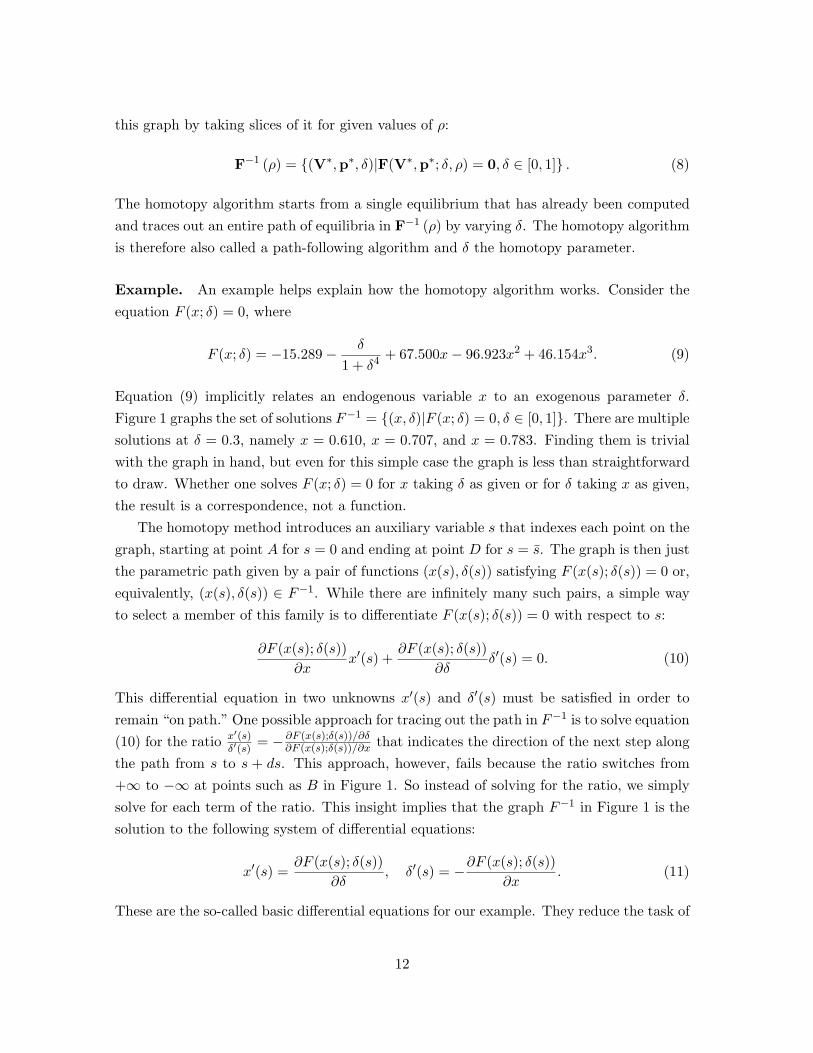
Example. An example helps explain how the homotopy algorithm works. Consider theequation F (x; δ) = 0, where

F (x; δ) = −15.289− δ

1 + δ4 + 67.500x− 96.923x2 + 46.154x3. (9)

Equation (9) implicitly relates an endogenous variable x to an exogenous parameter δ.Figure 1 graphs the set of solutions F−1 = {(x, δ)|F (x; δ) = 0, δ ∈ [0, 1]}. There are multiplesolutions at δ = 0.3, namely x = 0.610, x = 0.707, and x = 0.783. Finding them is trivialwith the graph in hand, but even for this simple case the graph is less than straightforwardto draw. Whether one solves F (x; δ) = 0 for x taking δ as given or for δ taking x as given,the result is a correspondence, not a function.

The homotopy method introduces an auxiliary variable s that indexes each point on thegraph, starting at point A for s = 0 and ending at point D for s = s. The graph is then justthe parametric path given by a pair of functions (x(s), δ(s)) satisfying F (x(s); δ(s)) = 0 or,equivalently, (x(s), δ(s)) ∈ F−1. While there are infinitely many such pairs, a simple wayto select a member of this family is to differentiate F (x(s); δ(s)) = 0 with respect to s:

∂F (x(s); δ(s))∂x

x′(s) +∂F (x(s); δ(s))

∂δδ′(s) = 0. (10)

This differential equation in two unknowns x′(s) and δ′(s) must be satisfied in order toremain “on path.” One possible approach for tracing out the path in F−1 is to solve equation(10) for the ratio x′(s)

δ′(s) = − ∂F (x(s);δ(s))/∂δ∂F (x(s);δ(s))/∂x that indicates the direction of the next step along

the path from s to s + ds. This approach, however, fails because the ratio switches from+∞ to −∞ at points such as B in Figure 1. So instead of solving for the ratio, we simplysolve for each term of the ratio. This insight implies that the graph F−1 in Figure 1 is thesolution to the following system of differential equations:

x′(s) =∂F (x(s); δ(s))

∂δ, δ′(s) = −∂F (x(s); δ(s))

∂x. (11)

These are the so-called basic differential equations for our example. They reduce the task of

12

tracing out the set of solutions to solving a system of differential equations. Given an initialcondition this can be done with a variety of methods (see Chapter 10 of Judd 1998). If δ = 0,then F (x; δ) = 0 is easily solved for x = 0.5, thereby providing an initial condition (pointA in Figure 1). From there the homotopy algorithm uses the basic differential equationsto determine the next step along the path. It continues to follow—step-by-step—the pathuntil it reaches δ = 1 (point D). In our example, the auxiliary variable s is decreasing frompoint A to point D. Therefore, whenever δ′(s) switches sign from negative to positive (pointB), the path is bending backward and there are multiple solutions. Conversely, wheneverthe sign of δ′(s) switches back from positive to negative (point C), the path is bendingforward.

Returning to our model of learning and forgetting, let x = (V∗,p∗) denote the 2M2

endogenous variables. Our goal is to explore F−1 (ρ), a slice of the graph of the equilibriumcorrespondence. Proceeding as in our example, a parametric path is a set of functions(x(s), δ(s)) ∈ F−1 (ρ). Differentiating F(x(s); δ(s), ρ) = 0 with respect to s yields thenecessary conditions for remaining on path:

∂F(x(s); δ(s), ρ)∂x

x′(s) +∂F(x(s); δ(s), ρ)

∂δδ′(s) = 0, (12)

where ∂F(x(s);δ(s),ρ)∂x is the (2M2 × 2M2) Jacobian, x′(s) and ∂F(x(s);δ(s),ρ)

∂δ are (2M2 × 1)vectors, and δ′(s) is a scalar. This system of 2M2 differential equations in the 2M2 + 1unknowns x′i(s), i = 1, . . . , 2M2, and δ′(s) has a solution that obeys the basic differentialequations:

y′i(s) = (−1)i+1 det((

∂F(y(s); ρ)∂y

)

−i

), i = 1, . . . , 2M2 + 1, (13)

where y(s) = (x(s), δ(s)) and the notation (·)−i is used to indicate that the ith column isremoved from the (2M2 × 2M2 + 1) Jacobian ∂F(y(s);ρ)

∂y . Note that equation (13) reducesto equation (11) if x is a scalar instead of a vector. Garcia & Zangwill (1979) and Chapter2 of Zangwill & Garcia (1981) prove that the basic differential equations (13) satisfy theconditions in equation (12).

The homotopy method requires that F(y; ρ) is continuously differentiable with respectto y and that the Jacobian ∂F(y;ρ)

∂y has full rank at all points in F−1(ρ). To appreciate the

importance of regularity, note that if the Jacobian ∂F(y(s);ρ)∂y has less than full rank at some

point y(s), then the determinants of all its (2M2 × 2M2) submatrices are zero. Hence,according to the basic differential equations (13), y′i(s) = 0 for i = 1, . . . , 2M2 + 1, and thealgorithm stalls. On the other hand, with regularity in place, the implicit function theoremensures that F−1(ρ) consists only of continuous paths; paths that suddenly terminate,

13

endless spirals, branch points, isolated equilibria, and continua of equilibria are ruled out(see Chapter 1 of Zangwill & Garcia 1981).

While our assumed functional forms ensure continuous differentiability, we have beenunable to establish regularity analytically. Indeed, we have numerical evidence suggestingthat regularity can fail. In practice, failures of regularity are not a problem as long as theyare confined to isolated points. Because our algorithm computes just a finite number ofpoints along the path, it is extremely unlikely to hit an irregular point.13 We refer thereader to Borkovsky, Doraszelski & Kryukov (2008) for a fuller discussion of this issue anda step-by-step guide to solving dynamic stochastic games using the homotopy method.

As Result 1 in Section 4 shows, we have always been able to trace out a path in F−1(ρ)that starts at the equilibrium for δ = 0 and ends at the equilibrium for δ = 1. Whenever this“main path” folds back on itself, the homotopy algorithm automatically identifies multipleequilibria. This makes it well-suited for models like ours that have multiple equilibria.

Nevertheless, the homotopy algorithm cannot be guaranteed to find all equilibria.14

The slice F−1 (ρ) may contain additional equilibria that are off the main path. Theseequilibria form one or more loops (see Result 1 in Section 4). We have two intuitivelyappealing but potentially fallible ways to try and identify additional equilibria. First, we usea large number of restarts of the P-M algorithm, often trying to “propagate” equilibria from“nearby” parameterizations. Second, and more systematically, just as we can choose δ asthe homotopy parameter while keeping ρ fixed, we can choose ρ while keeping δ fixed. Thisallows us to “crisscross” the parameter space in an orderly fashion by using the equilibria onthe δ-slices as initial conditions to generate ρ-slices. A ρ-slice must either intersect with allδ-slices or lead us to an additional equilibrium that, in turn, gives us an initial condition togenerate an additional δ-slice. We continue this process until all the ρ- and δ-slices “matchup”(for details see Grieco 2008).

3.2 Pakes & McGuire (1994) algorithm

While the homotopy method has advantages in finding multiple equilibria, it cannot standalone. The P-M algorithm (or some other means for solving a system of nonlinear equations)is necessary to compute a starting point for our homotopy algorithm.

Recall that V2(e) = V1(e[2]) and p2(e) = p1(e[2]) for each state e in a symmetric equi-librium and it therefore suffices to determine V and p, the value and policy functions offirm 1. The P-M algorithm is iterative. An iteration cycles through the states in somepredetermined order and updates V and p as it progresses from one iteration to the next.

13Our programs use Hompack (Watson, Billups & Morgan 1987, Watson, Sosonkina, Melville, Morgan &Walker 1997) written in Fortran 90. They are available from the authors upon request.

14Unless the system of equations that defines them happens to be polynomial; see Judd & Schmedders(2004) for some early efforts along this line.

14

The strategic situation firms face in setting prices in state e is similar to a static game ifthe value of continued play is taken as given. The P-M algorithm computes the best replyof firm 1 against p(e[2]) in this game and uses it to update the value and policy functionsof firm 1 in state e.

More formally, let h1(e, p1, p(e[2]),V) be the maximand in the Bellman equation (1)after symmetry is imposed. The best reply of firm 1 against p(e[2]) in state e is given by

G2e(V,p) = arg max

p1

h1(e, p1, p(e[2]),V) (14)

and the value associated with it is

G1e(V,p) = max

p1

h1(e, p1, p(e[2]),V). (15)

Write the collection of equations (14) and (15) for all states e ∈ {1, . . . , M}2 as

G(V,p) =

G1(1,1)(V,p)

G1(2,1)(V,p)

...G2

(M,M)(V,p)

. (16)

Given an initial guess x0 = (V0,p0), the P-M algorithm executes the iteration

xk+1 = G(xk), k = 0, 1, 2, . . . ,

until the changes in the value and policy functions of firm 1 are deemed small (or a failureto converge is diagnosed).

The P-M algorithm does not lend itself to computing multiple equilibria. To identifymore than one equilibrium (for a given parameterization of the model), it must be restartedfrom different initial guesses. But different initial guesses may or may not lead to differentequilibria. This, however, still understates the severity of the problem. Whenever ourdynamic stochastic game has multiple equilibria, the P-M algorithm cannot compute asubstantial fraction of them even if an arbitrarily large number of initial guesses are tried.

The problem is this. The P-M algorithm continues to iterate until it reaches a fixedpoint x = G (x). A necessary condition for convergence is local stability of the fixed point.Consider the (2M2×2M2) Jacobian ∂G(x)

∂x at the fixed point and let %(

∂G(x)∂x

)be its spectral

radius.15 The fixed point is locally stable under the P-M algorithm if %(

∂G(x)∂x

)< 1, i.e., if

15Let A be an arbitrary matrix and ς(A) the set of its eigenvalues. The spectral radius of A is %(A) =max {|λ| : λ ∈ ς(A)}.

15

all eigenvalues are within the complex unit circle. Given local stability, the P-M algorithmconverges provided that the initial guess is close (perhaps very close) to the fixed point.Conversely, if %

(∂G(x)

∂x

)≥ 1, then the fixed point is unstable and the P-M algorithm

cannot compute it. The following proposition identifies a subset of equilibria that the P-Malgorithm cannot compute.

Proposition 1 Let (x(s), δ(s)) ∈ F−1 (ρ) be a parametric path of equilibria. (i) If δ′(s) ≤ 0,

then %

(∂G(x(s))

∂x

∣∣∣(δ(s),ρ)

)≥ 1 and the equilibrium x(s) is unstable under the P-M algorithm.

(ii) Moreover, the equilibrium x(s) remains unstable with either dampening or extrapolationapplied to the P-M algorithm.

Part (i) of Proposition 1 establishes that the P-M algorithm cannot compute equilibriaon any part of the path for which δ′(s) ≤ 0. Whenever δ′(s) switches sign from positiveto negative, the main path connecting the equilibrium at δ = 0 with the equilibrium atδ = 1 bends backward and multiple equilibria arise. Conversely, whenever the sign of δ′(s)switches back from negative to positive, the main path bends forward. Hence, for a fixedforgetting rate δ (s), in between two equilibria for which δ′(s) > 0 lies a third—necessarilyunstable—equilibrium for which δ′(s) ≤ 0. Similarly, a loop has equilibria for which δ′(s) > 0and equilibria for which δ′(s) ≤ 0. Consequently, if we have multiple equilibria (for a givenparameterization of the model), then the P-M algorithm can compute at best 1/2 to 2/3 ofthem.

Dampening and extrapolation are often applied to the P-M algorithm in the hope ofimproving its likelihood or speed of convergence. The iteration

xk+1 = ωG(xk) + (1− ω)xk, k = 0, 1, 2, . . . ,

is said to be dampened if ω ∈ (0, 1) and extrapolated if ω ∈ (1,∞). Part (ii) of Proposition1 establishes the futility of these attempts.16

The ability of the P-M algorithm to provide a reasonably complete picture of the set ofsolutions to the model is limited beyond the scope of Proposition 1. Our numerical analysisindicates that the P-M algorithm cannot compute equilibria on some part of the path forwhich δ′(s) > 0:

Proposition 2 Let (x(s), δ(s)) ∈ F−1 (ρ) be a parametric path of equilibria. Even if δ′(s) >

0 we may have %

(∂G(x(s))

∂x

∣∣∣(δ(s),ρ)

)≥ 1 so that the equilibrium x(s) is unstable under the

P-M algorithm.16Dampening and extrapolation may, of course, still be helpful in computing equilibria for which δ′(s) > 0.

16

In the Online Appendix we prove Proposition 2 by way of an example and illustrate equi-libria of our model that the P-M algorithm cannot compute.

As is well-known, not all Nash equilibria of static games are stable under best reply dy-namics (see Chapter 1 of Fudenberg & Tirole 1991).17 Since the P-M algorithm incorporatesbest reply dynamics, it is reasonable to expect that this limits its usefulness. In the OnlineAppendix we argue that this is not the case. More precisely, we show that, holding fixedthe value of continued play, the best reply dynamics are contractive and therefore convergeto a unique fixed point irrespective of the initial guess. The value function iteration alsois contractive holding fixed the policy function. Hence, each of the two building blocks ofthe P-M algorithm “works.” What makes it impossible to obtain a substantial fraction ofequilibria is the interaction of value function iteration with best reply dynamics.

The P-M algorithm is a pre-Gauss-Jacobi method. The subsequent literature has in-stead sometimes used a pre-Gauss-Seidel method (Benkard 2004, Doraszelski & Judd 2008).Whereas a Gauss-Jacobi method replaces the old guesses for the value and policy functionswith the new guesses at the end of an iteration after all states have been visited, a Gauss-Seidel method updates after each state. This has the advantage that “information” isused as soon as it becomes available (see Chapters 3 and 5 of Judd 1998). We have beenunable to prove that Proposition 1 carries over to this alternative algorithm. We note,however, that the Stein-Rosenberg theorem (see Proposition 6.9 in Section 2.6 of Bertsekas& Tsitsiklis 1997) asserts that for certain systems of linear equations, if the Gauss-Jacobialgorithm fails to converge, then so does the Gauss-Seidel algorithm. Hence, it does notseem reasonable to presume that the Gauss-Seidel variant of the P-M algorithm is immuneto the difficulties the original algorithm suffers.

4 Equilibrium correspondence

This section provides an overview of the equilibrium correspondence. In the absence oforganizational forgetting, C-R establish uniqueness of equilibrium. Theorem 2.2 in C-Rextends to our model:

Proposition 3 If organizational forgetting is either absent (δ = 0) or certain (δ = 1), thenthere is a unique equilibrium.18

The cases of δ = 0 and δ = 1 are special in that they ensure that movements through thestate space are unidirectional. When δ = 0, a firm can never move “backward” to a lower

17More generally, in static games, Nash equilibria of degree −1 are unstable under any Nash dynamics,i.e., dynamics with rest points that coincide with Nash equilibria, including replicator and smooth fictitiousplay dynamics (Demichelis & Germano 2002).

18Proposition 3 pertains to both symmetric and asymmetric equilibria.

17

state and when δ = 1, it can never move “forward” to a higher state. Hence, backwardinduction can be used to establish uniqueness of equilibrium (see Section 7 for details). Incontrast, when δ ∈ (0, 1), a firm can move in either direction. These bidirectional movementsbreak the backward induction and make multiple equilibria possible:

Proposition 4 If organizational forgetting is neither absent (δ = 0) nor certain (δ = 1),then there may be multiple equilibria.

Figure 2 proves the proposition and illustrates the extent of multiplicity. It shows thenumber of equilibria that we have identified for each combination of progress ratio ρ andforgetting rate δ. Darker shades indicate more equilibria. As can be seen, we have foundup to nine equilibria for some values of ρ and δ. Multiplicity is especially pervasive forforgetting rates δ in the empirically relevant range below 0.1.

In dynamic stochastic games with finite actions, Herings & Peeters (2004) have shownthat generically the number of MPE is odd. While they consider both symmetric and asym-metric equilibria, in a two-player game with symmetric primitives such as ours, asymmetricequilibria occur in pairs. Hence, their result immediately implies that generically the num-ber of symmetric equilibria is odd in games with finite actions. Figure 2 suggests that thiscarries over to our setting with continuous actions.

In order to understand the geometry of how multiple equilibria arise we take a close lookat the slices of the graph of the equilibrium correspondence that our homotopy algorithmcomputes.

Result 1 The slice F−1 (ρ) contains a unique path that connects the equilibrium at δ = 0with the equilibrium at δ = 1. In addition, F−1 (ρ) may contain (one or more) loops thatare disjoint from this “main path” and from each other.

Figure 3 illustrates Result 1. To explain this figure, recall that an equilibrium consistsof a value function V∗ and a policy function p∗ and is thus an element of a high-dimensionalspace. To succinctly represent it, we proceed in two steps. First, we use p∗ to constructthe probability distribution over next period’s state e′ given this period’s state e, i.e., thetransition matrix that characterizes the Markov process of industry dynamics. We computethe transient distribution over states in period t, µt(·), starting from state (1, 1) in period 0.This tells us how likely each possible industry structure is in period t, given that both firmsbegan at the top of their learning curves. In addition, we compute the limiting (or ergodic)distribution over states, µ∞(·).19 The transient distributions capture short-run dynamicsand the limiting distribution captures long-run (or steady-state) dynamics.

19Let P be the M2 ×M2 transition matrix. The transient distribution in period t is given by µt = µ0Pt,where µ0 is the 1×M2 initial distribution and Pt the tth matrix power of P. If δ ∈ (0, 1), then the Markovprocess is irreducible because logit demand implies that the probability moving forward is always nonzero.

18

Second, we use the transient distribution over states in period t, µt(·), to compute theexpected Herfindahl index

Ht =∑e

(D∗

1(e)2 + D∗2(e)2

)µt(e).

The time path of Ht summarizes the implications of learning and forgetting for industrydynamics. If the industry evolves asymmetrically, then Ht > 0.5. The maximum expectedHerfindahl index

H∧ = maxt∈{1,...,100}

Ht

is a summary measure of short-run industry concentration. The limiting expected Herfind-ahl index H∞, computed using µ∞(·) instead of µt(·), is a summary measure of long-runindustry concentration. If H∞ > 0.5, then an asymmetric industry structure persists.

In Figure 3 we visualize F−1 (ρ) for a variety of progress ratios by plotting H∧ (dashedline) and H∞ (solid line). As can be seen, multiple equilibria arise whenever the main pathfolds back on itself. Moreover, there is one loop for ρ ∈ {0.75, 0.65, 0.55, 0.15, 0.05}, twoloops for ρ ∈ {0.85, 0.35}, and three loops for ρ = 0.95, thus adding further multiplicity.

Figure 3 is not necessarily a complete picture of the equilibria to our model. As discussedin Section 3.1, no algorithm is guaranteed to find all equilibria. We do find all equilibriaalong the main path and we have been successful in finding a number of loops. But otherloops may exist because, in order to trace out a loop, we must somehow compute at leastone equilibrium on the loop, and doing so is problematic.

Types of equilibria. Despite the multiplicity, the equilibria of our game exhibit thefour typical patterns shown in Figure 4.20 The parameter values are ρ = 0.85 and δ ∈{0, 0.0275, 0.08}; they represent the median progress ratio across a wide array of empiricalstudies combined with the cases of no, low, and high organizational forgetting. One shouldrecognize that the typical patterns, helpful as they are in understanding the range of be-haviors that can occur, lie on a continuum and thus morph into each other in complicatedways as we change the parameter values.

The upper left panel of Figure 4 is typical for what we call a flat equilibrium withoutwell (ρ = 0.85, δ = 0). The policy function is very even over the entire state space. Inparticular, the price that a firm charges in equilibrium is fairly insensitive to its rival’sstock of know-how. The upper right panel shows a flat equilibrium with well (ρ = 0.85,

That is, all its states belong to a single closed communicating class and the 1 × M2 limiting distributionµ∞ solves the system of linear equations µ∞ = µ∞P. If δ = 0 (δ = 1), then there is also a single closedcommunicating class, but its sole member is state (M, M) ((1, 1)).

20The value functions corresponding to the policy functions in Figure 4 can be found in the OnlineAppendix where we also provide tables of the value and policy functions for ease of reference.

19

δ = 0.0275). While the policy function remains even over most of the state space, pricecompetition is intense during the industry’s birth. This manifests itself as a “well” in theneighborhood of state (1, 1).

The lower left panel of Figure 4 exemplifies a trenchy equilibrium (ρ = 0.85, δ = 0.0275).The parameter values are the same as for the flat equilibrium with well, thereby providingan instance of multiplicity.21 The policy function is uneven and exhibits a “trench” alongthe diagonal of the state space. This trench starts in state (1, 1) and extends beyond thebottom of the learning curve in state (m, m) all the way to state (M, M). Hence, in atrenchy equilibrium, price competition between firms with similar stocks of know-how isintense but abates once firms become asymmetric. Finally, the lower right panel illustratesan extra-trenchy equilibrium (ρ = 0.85, δ = 0.08). The policy function has not only adiagonal trench but also trenches parallel to the edges of the state space. In these sidewaystrenches the leader competes aggressively with the follower.

Sunspots. For a progress ratio of ρ = 1 the marginal cost of production is constant atc(1) = . . . = c(M) = κ, and there are no gains from learning-by-doing. It clearly is anequilibrium for firms to disregard their stocks of know-how and set the same prices as in theNash equilibrium of a static price-setting game (obtained by setting β = 0). Since firms’marginal costs are constant, so are the static Nash equilibrium prices. Thus, we have anextreme example of a flat equilibrium with p∗(e) = κ + 2σ = 12 and V ∗(e) = σ

1−β = 21 forall states e ∈ {1, . . . , M}2.

Figure 2 shows that, in case of ρ = 1, there are two more equilibria for a range offorgetting rates δ below 0.1. Since the state of the industry has no bearing on the primitives,we refer to these equilibria as sunspots. One of the sunspots is a trenchy equilibrium whilethe other one is, depending on δ, either a flat or a trenchy equilibrium. In the trenchyequilibrium the industry evolves towards an asymmetric structure where the leader charges alower price than the follower and enjoys a higher probability of making a sale. Consequently,the net present value of cash flows to the leader exceeds that to the follower. The valuein state (1, 1), however, is lower than in the static Nash equilibrium, i.e., V ∗(1, 1) < 21.22

This indicates that value is destroyed as firms fight for dominance.The existence of sunspots and the fact that these equilibria persist for ρ ≈ 1 suggests

that the concept of MPE is richer than one may have thought. Besides describing the21As can be seen in the upper right panel of Figure 3, the main path in F−1(0.85) bends back on itself at

δ = 0.0275, and there are three equilibria for slightly lower values of δ and only one for slightly higher values.This particular parameterization (if not the pattern of behavior it generates) is therefore almost nongenericin that it approximates the isolated occurrence of an even number of equilibria. Due to the limited precisionof our homotopy algorithm, we have indeed been unable to find a third equilibrium.

22For example, if δ = 0.0275, then V ∗(28, 21) = 25.43 and p∗(28, 21) = 12.33 for the leader, V ∗(21, 28) =22.39 and p∗(21, 28) = 12.51 for the follower, and V ∗(1, 1) = 19.36.

20

physical environment of the industry the state serves as a summary of the history of play:A larger stock of know-how indicates that—on average—a firm has won more sales thanits rival, with the likely reason being that the firm has charged lower prices. Hence, byconditioning their current behavior on the state, firms implicitly condition on the historyof play. The difference with a subgame perfect equilibrium is that there firms have theentire history of play at their disposal whereas here they have but a crude indication of it.Nevertheless, “barely” payoff-relevant state variables (such as firms’ stocks of know-how ifρ ≈ 1) open the door for bootstrap-type equilibria as familiar from repeated games to arisein Markov-perfect settings.

In sum, accounting for organizational forgetting in a model of learning-by-doing leadsto multiple equilibria and a rich array of pricing behaviors. In the next section we explorewhat these behaviors entail for industry dynamics, both in the short run and in the longrun.

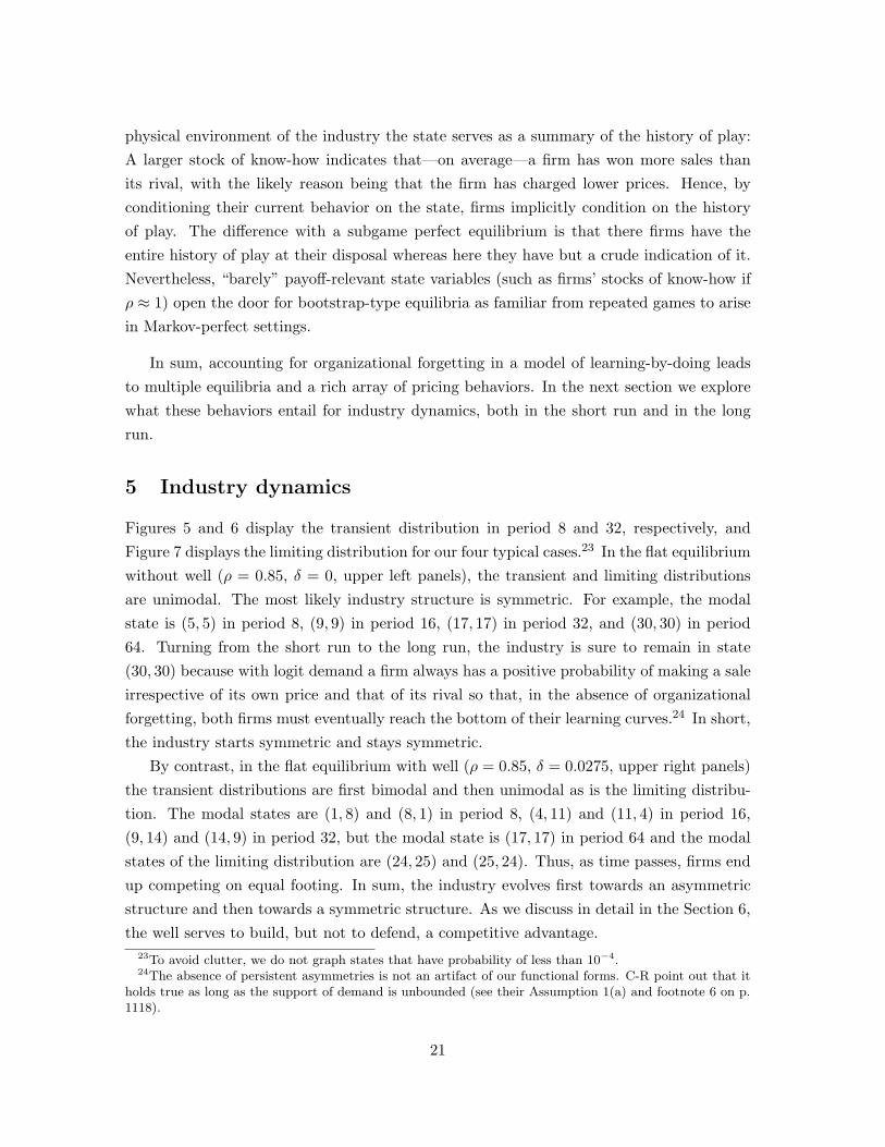
5 Industry dynamics

Figures 5 and 6 display the transient distribution in period 8 and 32, respectively, andFigure 7 displays the limiting distribution for our four typical cases.23 In the flat equilibriumwithout well (ρ = 0.85, δ = 0, upper left panels), the transient and limiting distributionsare unimodal. The most likely industry structure is symmetric. For example, the modalstate is (5, 5) in period 8, (9, 9) in period 16, (17, 17) in period 32, and (30, 30) in period64. Turning from the short run to the long run, the industry is sure to remain in state(30, 30) because with logit demand a firm always has a positive probability of making a saleirrespective of its own price and that of its rival so that, in the absence of organizationalforgetting, both firms must eventually reach the bottom of their learning curves.24 In short,the industry starts symmetric and stays symmetric.

By contrast, in the flat equilibrium with well (ρ = 0.85, δ = 0.0275, upper right panels)the transient distributions are first bimodal and then unimodal as is the limiting distribu-tion. The modal states are (1, 8) and (8, 1) in period 8, (4, 11) and (11, 4) in period 16,(9, 14) and (14, 9) in period 32, but the modal state is (17, 17) in period 64 and the modalstates of the limiting distribution are (24, 25) and (25, 24). Thus, as time passes, firms endup competing on equal footing. In sum, the industry evolves first towards an asymmetricstructure and then towards a symmetric structure. As we discuss in detail in the Section 6,the well serves to build, but not to defend, a competitive advantage.

23To avoid clutter, we do not graph states that have probability of less than 10−4.24The absence of persistent asymmetries is not an artifact of our functional forms. C-R point out that it

holds true as long as the support of demand is unbounded (see their Assumption 1(a) and footnote 6 on p.1118).

21

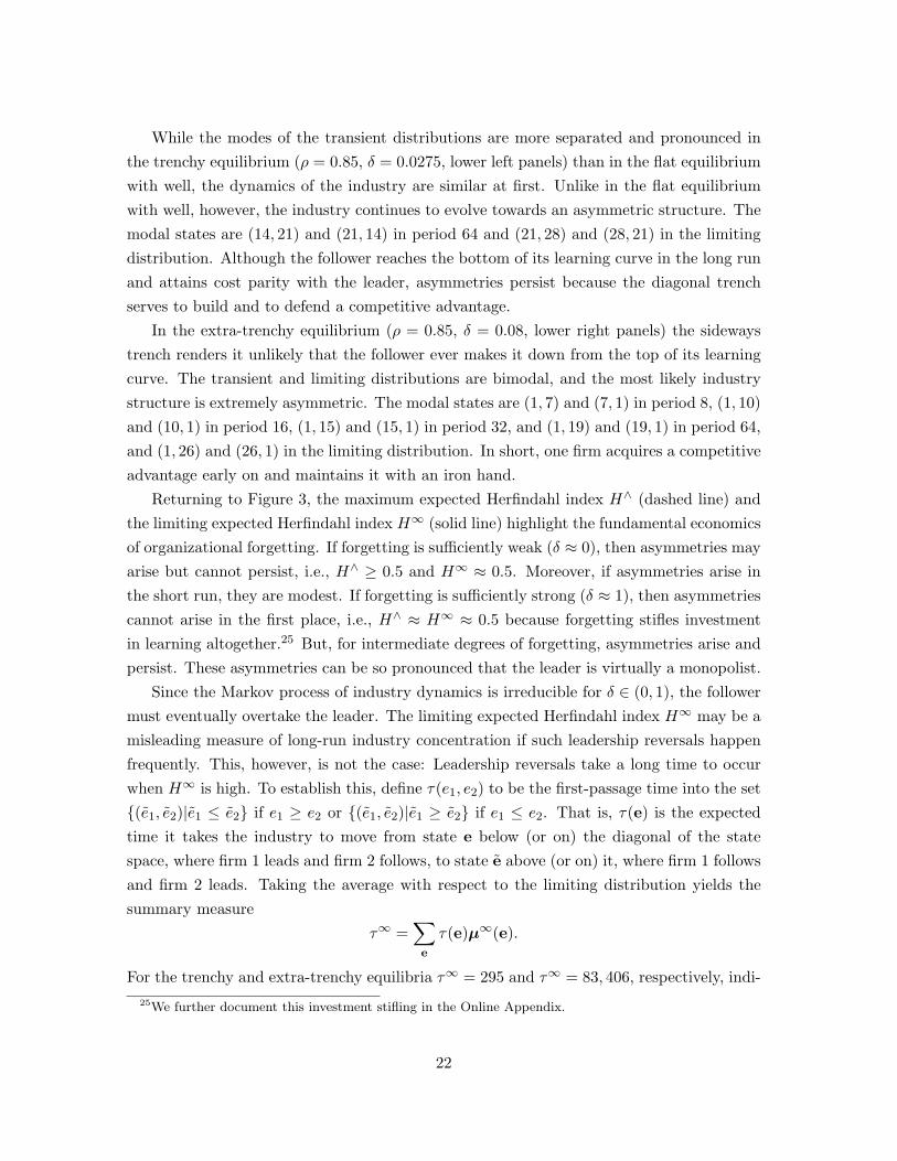
While the modes of the transient distributions are more separated and pronounced inthe trenchy equilibrium (ρ = 0.85, δ = 0.0275, lower left panels) than in the flat equilibriumwith well, the dynamics of the industry are similar at first. Unlike in the flat equilibriumwith well, however, the industry continues to evolve towards an asymmetric structure. Themodal states are (14, 21) and (21, 14) in period 64 and (21, 28) and (28, 21) in the limitingdistribution. Although the follower reaches the bottom of its learning curve in the long runand attains cost parity with the leader, asymmetries persist because the diagonal trenchserves to build and to defend a competitive advantage.

In the extra-trenchy equilibrium (ρ = 0.85, δ = 0.08, lower right panels) the sidewaystrench renders it unlikely that the follower ever makes it down from the top of its learningcurve. The transient and limiting distributions are bimodal, and the most likely industrystructure is extremely asymmetric. The modal states are (1, 7) and (7, 1) in period 8, (1, 10)and (10, 1) in period 16, (1, 15) and (15, 1) in period 32, and (1, 19) and (19, 1) in period 64,and (1, 26) and (26, 1) in the limiting distribution. In short, one firm acquires a competitiveadvantage early on and maintains it with an iron hand.

Returning to Figure 3, the maximum expected Herfindahl index H∧ (dashed line) andthe limiting expected Herfindahl index H∞ (solid line) highlight the fundamental economicsof organizational forgetting. If forgetting is sufficiently weak (δ ≈ 0), then asymmetries mayarise but cannot persist, i.e., H∧ ≥ 0.5 and H∞ ≈ 0.5. Moreover, if asymmetries arise inthe short run, they are modest. If forgetting is sufficiently strong (δ ≈ 1), then asymmetriescannot arise in the first place, i.e., H∧ ≈ H∞ ≈ 0.5 because forgetting stifles investmentin learning altogether.25 But, for intermediate degrees of forgetting, asymmetries arise andpersist. These asymmetries can be so pronounced that the leader is virtually a monopolist.

Since the Markov process of industry dynamics is irreducible for δ ∈ (0, 1), the followermust eventually overtake the leader. The limiting expected Herfindahl index H∞ may be amisleading measure of long-run industry concentration if such leadership reversals happenfrequently. This, however, is not the case: Leadership reversals take a long time to occurwhen H∞ is high. To establish this, define τ(e1, e2) to be the first-passage time into the set{(e1, e2)|e1 ≤ e2} if e1 ≥ e2 or {(e1, e2)|e1 ≥ e2} if e1 ≤ e2. That is, τ(e) is the expectedtime it takes the industry to move from state e below (or on) the diagonal of the statespace, where firm 1 leads and firm 2 follows, to state e above (or on) it, where firm 1 followsand firm 2 leads. Taking the average with respect to the limiting distribution yields thesummary measure

τ∞ =∑e

τ(e)µ∞(e).

For the trenchy and extra-trenchy equilibria τ∞ = 295 and τ∞ = 83, 406, respectively, indi-25We further document this investment stifling in the Online Appendix.

22

cating that a leadership reversal takes a long time to occur. Hence, the asymmetry capturedby H∞ persists. In the Online Appendix we plot the expected time to a leadership reversalτ∞ in the same format as Figure 3. Just like H∞, τ∞ is largest for intermediate degrees offorgetting. Moreover, τ∞ is of substantial magnitude, easily reaching and exceeding 1, 000periods. Asymmetries are therefore persistent in our model because the expected time untilthe leader and the follower switch roles is (perhaps very) long.

We caution the reader that the absence of persistent asymmetries for small forgettingrates δ in Figure 3 may be an artifact of the finite size of the state space (M = 30 in ourbaseline parameterization). Given δ = 0.01, say, ∆(30) = 0.26 and organizational forgettingis so weak that the industry is sure to remain in or near state (30, 30). This eliminatesbidirectional movements sufficiently completely so as to restore the backward inductionlogic that underlies uniqueness of equilibrium for the extreme case of δ = 0 (see Proposition3). We show in the Online Appendix that, increasing M , whilst holding fixed δ, facilitatespersistent asymmetries as the industry becomes more likely to remain in the interior of thestate space. Furthermore, as emphasized in Section 1, shut-out model elements can giverise to persistent asymmetries even in the absence of organizational forgetting. We explorethis issue further in Section 8.

To summarize, contrary to what one might expect, organizational forgetting does notnegate learning-by-doing. Rather, as can be seen in Figure 3, over a range of progress ratiosρ above 0.6 and forgetting rates δ below 0.1, learning and forgetting reinforce each other.Starting from the absence of both learning (ρ = 1) and forgetting (δ = 0), a steeper learningcurve (lower progress ratio) tends to give rise to a more asymmetric industry structure justas a higher forgetting rate does. In the next section we analyze the pricing behavior thatdrives these dynamics.

6 Pricing behavior

Re-writing equation (5) shows that firm 1’s price in state e satisfies

p∗(e) = c∗(e) +σ

1−D∗1(e)

, (17)

where the virtual marginal cost,

c∗(e) = c(e1)− βφ∗(e), (18)

equals the actual marginal cost, c(e1), minus the discounted prize, βφ∗(e), from winning thecurrent period’s sale. The prize, in turn, is the difference in the value of continued play to

23

firm 1 if it wins the sale, V∗1(e), versus if it loses the sale, V

∗2(e):

φ∗(e) = V∗1(e)− V

∗2(e). (19)

Note that, irrespective of the forgetting rate δ, the equilibrium of our dynamic stochasticgame reduces to the static Nash equilibrium if firms are myopic. Setting β = 0 in equations(17) and (18) gives the usual FOC for a static price-setting game with logit demand:

p†(e) = c(e1) +σ

1−D†1(e)

, (20)

where D†k(e) = Dk(p†(e), p†(e[2])) denotes the probability that, in the static Nash equilib-

rium, the buyer purchases from firm k ∈ {1, 2} in state e. Thus, if β = 0, then p∗(e) = p†(e)and V ∗(e) = D†

1(e)(p†(e)− c(e1)

)for all states e ∈ {1, . . . , M}2.

6.1 Price bounds

Comparing equations (17) and (20) shows that equilibrium prices p∗(e) and p∗(e[2]) coincidewith the prices that obtain in a static Nash equilibrium with costs equal to virtual marginalcosts c∗(e) and c∗(e[2]). Static Nash equilibrium prices are increasing in either firm’s cost(Vives 1999, p. 35). Therefore, if both firms’ prizes are nonnegative, static Nash equilibriumprices are an upper bound on equilibrium prices, i.e., if φ∗(e) ≥ 0 and φ∗(e[2]) ≥ 0, thenp∗(e) ≤ p†(e) and p∗(e[2]) ≤ p†(e[2]).

A sufficient condition for φ∗(e) ≥ 0 for each state e is that the value function V ∗(e)is nondecreasing in e1 and nonincreasing in e2. Intuitively, it should not hurt firm 1 if itmoves down its learning curve and it should not benefit firm 1 if firm 2 moves down itslearning curve. While neither we nor C-R have succeeded in proving it, our computationsshow that this intuition is valid in the absence of organizational forgetting:

Result 2 If organizational forgetting is absent (δ = 0), then p∗(e) ≤ p†(e) for all e ∈{1, . . . , M}2.

Result 2 highlights the fundamental economics of learning-by-doing: As long as improve-ments in competitive position are valuable, firms use price cuts as investments to achievethem.

We complement Result 2 by establishing a lower bound on equilibrium prices in stateswhere at least one of the two firms has reached the bottom of its learning curve:

Proposition 5 If organizational forgetting is absent (δ = 0), then (i) p∗(e) = p†(e) =p†(m, m) > c(m) for all e ∈ {m, . . . , M}2 and (ii) p∗(e) > c(m) for all e1 ∈ {m, . . . , M}and e2 ∈ {1, . . . , m− 1}.

24

Part (i) of Proposition 5 sharpens Theorem 4.3 in C-R by showing that once both firmshave reached the bottom of their learning curves, equilibrium prices revert to static Nashlevels. To see why, note that, given δ = 0, the prize reduces to φ∗(e) = V ∗(e1 + 1, e2) −V ∗(e1, e2 +1). But beyond the bottom of their learning curves, firms’ competitive positionscan neither improve nor deteriorate. Hence, as we show in the proof of the proposition,V ∗(e) = V ∗(e′) for all e, e′ ∈ {m, . . . , M}2, so that the advantage-building and advantage-defending motives disappear, the prize is zero, and equilibrium prices revert to static Nashlevels. This rules out trenches penetrating into this region of the state space. Trenchy andextra-trenchy equilibria therefore cannot arise in the absence of organizational forgetting.

Part (ii) of Proposition 5 restates Theorem 4.3 in C-R for the situation where the leaderbut not the follower has reached the bottom of its learning curve. The leader no longer hasan advantage-building motive but continues to have an advantage-defending motive. Thisraises the possibility that the leader uses price cuts to delay the follower in moving down itslearning curve. The proposition shows that there is a limit to how aggressively the leaderdefends its advantage: below-cost pricing is never optimal in the absence of organizationalforgetting.

The story changes dramatically in the presence of organizational forgetting. The equi-librium may exhibit soft competition in some states and price wars in other states. Considerthe trenchy equilibrium (ρ = 0.85, δ = 0.0275). The upper bound in Result 2 fails in state(22, 20) where the leader charges 6.44 and the follower charges 7.60, significantly above itsstatic Nash equilibrium price of 7.30. The follower’s high price stems from its prize of −1.04.This prize, in turn, reflects that, if the follower wins the sale, then the industry most likelymoves to state (22, 21) and thus closer to the brutal price competition on the diagonal ofthe state space. Indeed, the follower’s value function decreases from 20.09 in state (22, 20)to 19.56 in state (22, 21). To avoid this undesirable possibility, the follower charges a highprice. The lower bound in Proposition 5 fails in state (20, 20) where both firms charge 5.24as compared to a marginal cost of 5.30. The prize of 2.16 makes it worthwhile to pricebelow cost even beyond the bottom of the learning curve because “in the trench” winningthe current sale confers a lasting advantage.

This discussion provides the instances that prove the next two propositions.

Proposition 6 If organizational forgetting is present (δ > 0), then we may have p∗(e) >

p†(e) for some e ∈ {1, . . . , M}2.

Figure 8 illustrates Proposition 6 by plotting the share of equilibria that violate the upperbound in Result 2.26 Darker shades indicate higher shares. As can be seen, the upper

26To take into account the limited precision of our computations, we take the upper bound to be violatedif p∗(e) > p†(e) + ε for some e ∈ {1, . . . , M}2, where ε is positive but small. Specifically, we set ε = 10−2, so

25

bound continues to hold if organizational forgetting is very weak (δ ≈ 0) and possibly alsoif learning-by-doing is very weak (ρ ≈ 1). Apart from these extremes (and a region aroundρ = 0.45 and δ = 0.25), at least some, if not all, equilibria entail at least one state whereequilibrium prices exceed static Nash equilibrium prices.

Taken alone, Proposition 6 suggests that organizational forgetting makes firms less ag-gressive. This makes sense: After all, why invest in improvements in competitive positionwhen they are transitory? But organizational forgetting can also be a source of aggressivepricing behavior:

Proposition 7 If organizational forgetting is present (δ > 0), then we may have p∗(e) ≤c (m) for some e1 ∈ {m, . . . ,M} and e2 ∈ {1, . . . , M}.

Figure 9 illustrates Proposition 7 by plotting the share of equilibria in which a firm pricesbelow cost even though it has reached the bottom of its learning curve. Note that Figure 9is a conservative tally of how often the lower bound in Proposition 5 fails because the lowerbound in part (i) already fails if the leader charges less than its static Nash equilibrium price,not less than its marginal cost. In sum, the leader may be more aggressive in defendingits advantage in the presence of organizational forgetting than in its absence. The mostdramatic expression of this aggressive pricing behavior are the diagonal trenches that arethe defining feature of trenchy and extra-trenchy equilibria.

6.2 Wells and trenches

This section develops intuition as to how wells and trenches can arise. Our goal is to provideinsight as to whether equilibria featuring wells and trenches are economically plausible and,at least potentially, empirically relevant.

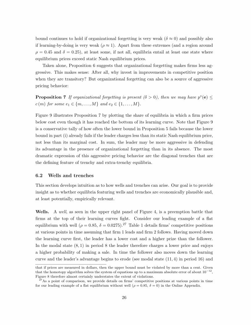
Wells. A well, as seen in the upper right panel of Figure 4, is a preemption battle thatfirms at the top of their learning curves fight. Consider our leading example of a flatequilibrium with well (ρ = 0.85, δ = 0.0275).27 Table 1 details firms’ competitive positionsat various points in time assuming that firm 1 leads and firm 2 follows. Having moved downthe learning curve first, the leader has a lower cost and a higher prize than the follower.In the modal state (8, 1) in period 8 the leader therefore charges a lower price and enjoysa higher probability of making a sale. In time the follower also moves down the learningcurve and the leader’s advantage begins to erode (see modal state (11, 4) in period 16) and

that if prices are measured in dollars, then the upper bound must be violated by more than a cent. Giventhat the homotopy algorithm solves the system of equations up to a maximum absolute error of about 10−12,Figure 8 therefore almost certainly understates the extent of violations.

27As a point of comparison, we provide details on firms’ competitive positions at various points in timefor our leading example of a flat equilibrium without well (ρ = 0.85, δ = 0) in the Online Appendix.

26

modal leader followerperiod state cost prize price prob. value cost prize price prob. value

0 (1,1) 10.00 6.85 5.48 0.50 5.87 10.00 6.85 5.48 0.50 5.878 (8,1) 6.14 3.95 7.68 0.81 22.99 10.00 2.20 9.14 0.19 5.3416 (11,4) 5.70 1.16 7.20 0.62 20.08 7.22 1.23 7.68 0.38 11.4832 (14,9) 5.39 0.36 7.16 0.53 20.06 5.97 0.64 7.27 0.47 17.3064 (17,17) 5.30 -0.01 7.31 0.50 20.93 5.30 -0.01 7.31 0.50 20.93∞ (25,24) 5.30 -0.01 7.30 0.50 21.02 5.30 -0.00 7.30 0.50 21.02

Table 1: Cost, prize, price, probability of making a sale, and value. Flat equilibrium withwell (ρ = 0.85, δ = 0.0275).

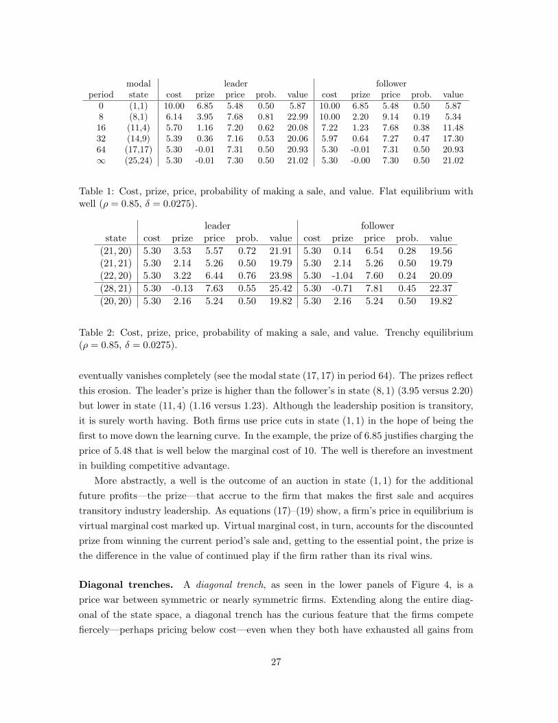
leader followerstate cost prize price prob. value cost prize price prob. value

(21, 20) 5.30 3.53 5.57 0.72 21.91 5.30 0.14 6.54 0.28 19.56(21, 21) 5.30 2.14 5.26 0.50 19.79 5.30 2.14 5.26 0.50 19.79(22, 20) 5.30 3.22 6.44 0.76 23.98 5.30 -1.04 7.60 0.24 20.09(28, 21) 5.30 -0.13 7.63 0.55 25.42 5.30 -0.71 7.81 0.45 22.37(20, 20) 5.30 2.16 5.24 0.50 19.82 5.30 2.16 5.24 0.50 19.82

Table 2: Cost, prize, price, probability of making a sale, and value. Trenchy equilibrium(ρ = 0.85, δ = 0.0275).

eventually vanishes completely (see the modal state (17, 17) in period 64). The prizes reflectthis erosion. The leader’s prize is higher than the follower’s in state (8, 1) (3.95 versus 2.20)but lower in state (11, 4) (1.16 versus 1.23). Although the leadership position is transitory,it is surely worth having. Both firms use price cuts in state (1, 1) in the hope of being thefirst to move down the learning curve. In the example, the prize of 6.85 justifies charging theprice of 5.48 that is well below the marginal cost of 10. The well is therefore an investmentin building competitive advantage.

More abstractly, a well is the outcome of an auction in state (1, 1) for the additionalfuture profits—the prize—that accrue to the firm that makes the first sale and acquirestransitory industry leadership. As equations (17)–(19) show, a firm’s price in equilibrium isvirtual marginal cost marked up. Virtual marginal cost, in turn, accounts for the discountedprize from winning the current period’s sale and, getting to the essential point, the prize isthe difference in the value of continued play if the firm rather than its rival wins.

Diagonal trenches. A diagonal trench, as seen in the lower panels of Figure 4, is aprice war between symmetric or nearly symmetric firms. Extending along the entire diag-onal of the state space, a diagonal trench has the curious feature that the firms competefiercely—perhaps pricing below cost—even when they both have exhausted all gains from

27

learning-by-doing. Part (i) of Proposition 5 rules out this type of behavior in the absenceof organizational forgetting.

Like a well, a diagonal trench serves to build a competitive advantage. Unlike a well, adiagonal trench also serves to defend a competitive advantage, thereby rendering it (almost)permanent: The follower recognizes that to seize the leadership position it would have to“cross over” the diagonal trench and struggle through another price war. Crucially thisprice war is a part of a MPE and, as such, a credible threat the follower cannot ignore.

The logic behind a diagonal trench has three parts. If a diagonal trench exists, thenthe follower does not contest the leadership position. If the follower does not contest theleadership position, then being the leader is valuable. Finally, to close the circle of logic,if being the leader is valuable, then firms price aggressively on the diagonal on the statespace in a bid for the leadership position, thus giving rise to the diagonal trench. Table2 illustrates this argument by providing details on firms’ competitive position in variousstates for our leading example of a trenchy equilibrium (ρ = 0.85, δ = 0.0275).

Part 1: Trench sustains leadership. To see why the follower does not contest the leader-ship position consider a state such as (21, 20) where the follower has almost caught up withthe leader. Suppose the follower wins the current sale. In this case the follower may leapfrogthe leader if the industry moves against the odds to state (20, 21). However, the most likelypossibility, with a probability of 0.32, is that the industry moves to state (21, 21). Due tothe brutal price competition “in the trench” the follower’s expected cash flow in the nextperiod decreases to −0.02 = 0.50×(5.26−5.30) compared to 0.34 = 0.28×(6.54−5.30) if theindustry had remained in state (21, 20). Suppose, in contrast, the leader wins. This com-pletely avoids sparking a price war. Moreover, the most likely possibility, with a probabilityof 0.32, is that the leader enhances its competitive advantage by moving to state (22, 20). Ifso, the leader’s expected cash flow in the next period increases to 0.87 = 0.76×(6.44−5.30)compared to 0.20 = 0.72× (5.57− 5.30) if the industry had remained in state (21, 20). Be-cause winning the sale is more valuable to the leader than to the follower, the leader’s prizein state (21, 20) is almost 25 times larger than the follower’s and the leader underprices thefollower. As a consequence, the leader defends its position with a substantial probability of0.79. In other words, the diagonal trench sustains the leadership position.

Part 2: Leadership generates value. Because the leader underprices the follower, overtime the industry moves from state (21, 20) to (or near) the modal state (28, 21) of thelimiting distribution. Once there the leader underprices the follower (7.63 versus 7.81)despite cost parity and thus enjoys a higher probability of making a sale (0.55 versus 0.45).The leader’s expected cash flow in the current period is therefore 0.55× (7.63−5.30) = 1.27as compared to the follower’s of 0.45× (7.81− 5.30) = 1.14. Because the follower does notcontest the leadership position, the leader is likely to enjoy these additional profits for a

28

leader followerstate cost prize price prob. value cost prize price prob. value(26, 1) 5.30 6.43 8.84 0.90 53.32 10.00 0.12 11.00 0.10 2.42(26, 2) 5.30 6.21 7.48 0.88 46.31 8.50 0.21 9.44 0.12 2.55(26, 3) 5.30 5.16 6.94 0.85 40.23 7.73 0.27 8.65 0.15 2.78

......

......

......

......

......

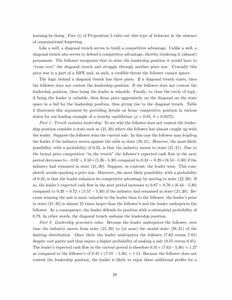
...(26, 7) 5.30 3.04 6.14 0.73 24.76 6.34 0.58 7.15 0.27 4.16(26, 8) 5.30 2.33 5.99 0.66 21.86 6.14 1.08 6.64 0.34 4.78(26, 9) 5.30 1.17 6.24 0.51 19.84 5.97 1.71 6.29 0.49 6.07(26, 10) 5.30 0.16 6.83 0.40 19.09 5.83 1.96 6.44 0.60 8.08

Table 3: Cost, prize, price, probability of making a sale, and value. Extra-trenchy equilib-rium (ρ = 0.85, δ = 0.08).

long time (recall that τ∞ = 295). Hence, being the leader is valuable.Part 3: Value induces trench. Because being the leader is valuable, firms price aggres-

sively on the diagonal on the state space in a bid for the leadership position. The prizeis 2.16 in state (20, 20) and 2.14 in state (21, 21) and justifies charging a price of 5.24 and5.26, respectively, even through all gains from learning-by-doing have been exhausted. Thisgives rise to the diagonal trench. Observe that this argument applies at every state onthe diagonal because, no matter where on the diagonal the firms happen to be, winningthe current sale confers a lasting advantage. The trench therefore extends along the entirediagonal of the state space.

All this can be summed up in a sentence: Building a competitive advantage creates thediagonal trench that defends the advantage and creates the prize that makes it worthwhileto fight for the leadership position. A diagonal trench is thus a self-reinforcing mechanismfor gaining and maintaining market dominance.

Sideways trenches. A sideways trench, as seen in the lower right panel of Figure 4, is aprice war between very asymmetric firms. This war is triggered when the follower starts tomove down its learning curve. Table 3 provides details on firms’ competitive positions invarious states for our leading example of an extra-trenchy equilibrium (ρ = 0.85, δ = 0.08).The sideways trench is evident in the decrease in the leader’s price from state (26, 1) tostate (26, 8) and the increase from state (26, 8) to state (26, 10). Note that the follower haslittle chance of making it down its learning curve as long as the probability of winning a saleis less than the probability of losing a unit of know-how through organizational forgetting.While D∗

2(26, 1) = 0.10 > 0.08 = ∆(1), we have D∗2(26, 2) = 0.12 < 0.15 = ∆(2) and

D∗2(26, 3) = 0.15 < 0.22 = ∆(3). Hence, the leader can stall the follower at the top of its

29

learning curve and, indeed, the modal state of the limiting distribution is (26, 1).The additional future profits stemming from the leader’s ability to stall the follower are

the source of its large prize in state (26, 1). In state (26, 2) the prize is almost as largebecause by winning a sale the leader may move the industry back to state (26, 1) in thenext period. The leader’s prize falls as the follower moves further down its learning curvebecause it takes progressively longer for the leader to force the follower back up its learningcurve and because the lower cost of the follower makes it harder for the leader to do so. Inthe unlikely event that the follower crashes through the sideways trench in state (26, 8), theleader’s prize falls sharply. At the same time the follower’s prize rises sharply as it turnsfrom a docile competitor into a viable threat.

A sideways trench, like a diagonal trench, is a self-reinforcing mechanism for gainingand maintaining market dominance. But whereas a diagonal trench is about fighting animminent threat, a sideways trench is about fighting a distant threat. One can think of asideways trench as an endogenously arising mobility barrier in the sense of Caves & Porter(1977) or the equilibrium manifestation of former Intel CEO Andy Grove’s dictum “Onlythe paranoid survive.”

In sum, the four types of equilibria that we have identified in Section 4 give rise todistinct yet plausible pricing behaviors and industry dynamics. Rather than impedingaggressive behavior, organizational forgetting facilitates it. In its absence, the equilibriaare flat either with or without well depending on the progress ratio. Generally speaking,organizational forgetting is associated with “trenchier” equilibria, more aggressive behavior,and more concentrated industries both in the short run and in the long run.

6.3 Dominance properties

Traditional intuition suggests that learning-by-doing leads by itself to market dominanceby giving a more experienced firm the ability to profitably underprice its less experiencedrival. This enables the leader to widen its competitive advantage over time, thereby furtherenhancing its ability to profitably underprice the follower. C-R formalize this idea with“two concepts of self-reinforcing market dominance” (p. 1115): An equilibrium exhibitsincreasing dominance (ID) if p∗(e)−p∗(e[2]) < 0 whenever e1 > e2 and increasing increasingdominance (IID) if p∗(e)−p∗(e[2]) is decreasing in e1. If ID holds, the leader charges a lowerprice than the follower and therefore enjoys a higher probability of making a sale. If IIDholds, the price gap between the firms widens with the length of the lead.28

28Athey & Schmutzler’s (2001) notion of weak increasing dominance describes the relationship betweenplayers’ states and their actions in dynamic games with deterministic state-to-state transitions and coincideswith the notion of ID in C-R. Similar notions have also been used by Vickers (1986) and Budd, Harris &Vickers (1993) in dynamic investment games.

30

In the absence of organizational forgetting, Theorem 3.3 in C-R shows that ID and IIDhold provided that the discount factor β is sufficiently close to 1 (or, alternatively, to 0, seeTheorem 3.1 in C-R). Our computations show that β = 1

1.05 in our baseline parameterizationsuffices.

Result 3 If organizational forgetting is absent (δ = 0), then IID holds. Thus, ID holds.

Even if an equilibrium satisfies ID and IID it is not clear that the industry is inevitablyprogressing towards monopolization. If the price gap between the firms is small, then theimpact of ID and IID on industry structure and dynamics may be trivial.29 In such ascenario, the leader charges a slightly lower price than the follower and this gap widens abit over time. However, with even a modest degree of horizontal product differentiation,the firms still split sales more or less equally and thus move down the learning curve intandem. This is exactly what happens when δ = 0. For example, the flat equilibriumwithout well (ρ = 0.85, δ = 0) satisfies IID and thus ID, but with a maximum expectedHerfindahl index of 0.52 the industry is essentially a symmetric duopoly at all times. Moregenerally, as Figure 3 shows, in the absence of organizational forgetting asymmetries aremodest if they arise at all. Although ID and IID hold, the maximum expected Herfindahlindex across all equilibria is 0.67 (attained at ρ = 0.65). Hence, ID and IID are not sufficientfor economically meaningful market dominance.

ID and IID are also not necessary for market dominance. The extra-trenchy equilibrium(ρ = 0.85, δ = 0.08), for example, violates ID and thus IID. Yet, the industry is likelyto be a near-monopoly at all times. More generally, while the empirical studies of Argoteet al. (1990), Darr et al. (1995), Benkard (2000), Shafer et al. (2001), and Thompson (2003)warrant accounting for organizational forgetting in a model of learning-by-doing, doing somay cause ID and IID to fail.

Proposition 8 If organizational forgetting is present (δ > 0), then IID may fail. Also IDmay fail.

In the absence of organizational forgetting, C-R have already shown that ID and IID mayfail for intermediate values of β (see their Remark C.5 on p. 1136). Result 3 and Proposition8 make the comparative dynamics point that ID and IID may hold when δ = 0 but failwhen δ > 0 (holding fixed the remaining parameters). Figure 10 illustrates Proposition 8by plotting the share of equilibria that violate IID (upper panel) and ID (lower panel). Ascan be seen, all equilibria fail to obey IID unless forgetting or learning is very weak. Even

29Indeed, C-R show in their Theorem 3.2 that p∗(e) → p†(m, m) for all e ∈ {1, . . . , M}2 as β → 1, i.e.,both firms price as if at the bottom of their learning curves. This suggests that the price gap may be smallfor “reasonable” discount factors.

31

flat eqbm.withoutwell

flat eqbm.with well

trenchyeqbm.

extra-trenchyeqbm.

leading example ρ = 0.85, ρ = 0.85, ρ = 0.85, ρ = 0.85,δ = 0 δ = 0.0275 δ = 0.0275 δ = 0.08

preemption battle (well) no yes no noprice war triggered by immi-nent threat (diagonal trench)

no no yes yes

price war triggered by distantthreat (sideways trench)

no no no yes

short-run market dominance no yes yes yeslong-run market dominance no no yes, yes,

modest extremedominance properties yes no, no, no,

mostly mostly mostly

Table 4: Pricing behavior and industry dynamics.

violations of ID are extremely common, especially for forgetting rates δ in the empiricallyrelevant range below 0.1.

Of course, we do not argue that the concepts of ID and IID have no place in theanalysis of industry dynamics. Caution, however, is advisable. Since ID and IID are neithernecessary nor sufficient for market dominance, making inferences about the evolution of theindustry on their basis alone may be misleading.

6.4 Summary

Table 4 summarizes the broad patterns of pricing behavior and industry dynamics. Acknowl-edging that the know-how gained through learning-by-doing can be lost through organiza-tional forgetting is important. Generally speaking, organizational forgetting is associatedwith “trenchier” equilibria, more aggressive behavior, and more concentrated industriesboth in the short run and in the long run. Moreover, the dominance properties of firms’pricing behavior can break down in the presence of organizational forgetting.

The key difference between a model with and without organizational forgetting is thatin the former a firm can move both forward to a higher state and backward to a lower state.This possibility of bidirectional movement enhances the advantage-building and advantage-defending motives. By winning a sale, a firm makes itself less, and its rival more, vulnerableto organizational forgetting. This can create strong incentives to cut prices. Rather thanimpeding it, organizational forgetting therefore facilitates aggressive pricing as manifestedin the trenchy and extra-trenchy equilibria that we have identified.

32

7 Organizational forgetting and multiple equilibria

While the equilibrium is unique if organizational forgetting is either absent (δ = 0) or certain(δ = 1), multiple equilibria are common for intermediate degrees of forgetting. Surprisingly,for some values of ρ and δ, the equilibria range from “peaceful coexistence” to “trenchwarfare.” Consequently, in addition to primitives of learning-by-doing and organizationalforgetting, the equilibrium by itself is an important determinant of pricing behavior andindustry dynamics.

Why do multiple equilibria arise in our model? To explore this question, think about thestrategic situation faced by firms in setting prices in state e. The value of continued playto firm n is given by the conditional expectation of its value function, V n1(e) and V n2(e),as defined in equations (2) and (3). Holding the value of continued play fixed, the strategicsituation in state e is akin to a static game. If the reaction functions in this game intersectmore than once, then multiple equilibria arise. On the other hand, if they intersect onlyonce irrespective of the value of continued play, then we say that a model satisfies statewiseuniqueness.

Proposition 9 Statewise uniqueness holds.

Not surprisingly the proof of Proposition 9 relies on the functional form of demand. Thisis reminiscent of the restrictions on demand (e.g., log-concavity) that Caplin & Nalebuff(1991) set forth to guarantee uniqueness of Nash equilibrium in their analysis of staticprice-setting games.

Given that the model satisfies statewise uniqueness, multiple equilibria must arise fromfirms’ expectations regarding the value of continued play. To see this, consider again statee. The intersection of the reaction functions constitutes a Nash equilibrium in prices in asubgame in which firm n believes that its value of continued play is given by V n1(e) andV n2(e). If firms have rational expectations, i.e., if the conjectured value of continued playis actually attained, then these prices constitute an equilibrium of our dynamic stochasticgame. In our model, taking the value of continued play as given, the reaction functionsintersect only once because we have statewise uniqueness, but there may be more thanone value of continued play that is consistent with rational expectations. In this sensemultiplicity is rooted in the dynamics of the model.

The key driver of multiplicity is organizational forgetting. Dynamic competition withlearning and forgetting is like racing down an upward-moving escalator. Unless a firmmakes sales at a rate that exceeds the rate at which it loses know-how through forgetting,its marginal cost is bound to increase. The inflow of know-how into the industry is oneunit per period whereas in expectation the outflow in state e is ∆(e1) + ∆(e2). Consider

33

state (e, e), where e ≥ m, on the diagonal of the state space at or beyond the bottom ofthe learning curve. If 1 ¿ 2∆(e), then it is impossible that both firms reach the bottomof their learning curves and remain there. Knowing this, firms have no choice but to priceaggressively. The result is trench warfare as each firm uses price cuts to push the stateto its side of the diagonal and keep it there. If, however, 1 À 2∆(e), then it is virtuallyinevitable that both firms reach the bottom of their learning curves, and firms may as wellprice softly. In both cases, the primitives of the model tie down the equilibrium.

This is no longer the case if 1 ≈ 2∆(e), setting the stage for multiple equilibria as diverseas peaceful coexistence and trench warfare. If firms believe that they cannot peacefullycoexist at the bottom of their learning curves and that one firm will come to dominatethe market, then both firms will cut their prices in the hope of acquiring a competitiveadvantage early on and maintaining it throughout. This naturally leads to trench warfareand market dominance. If, however, firms believe that they can peacefully coexist at thebottom of their learning curves, then neither firm cuts its price. Soft pricing, in turn,ensures that the anticipated symmetric industry structure actually emerges. A back-of-the-envelope calculation is reassuring here. Recall that m = 15 and M = 30 in our baselineparameterization and observe that 1 = 2∆(15) implies δ ≈ 0.045, 1 = 2∆(20) impliesδ ≈ 0.034, and 1 = 2∆(30) implies δ ≈ 0.023. This range of forgetting rates, for which theinflow of know-how approximately equals the outflow, is indeed where multiplicity prevails(see again Figure 2).

A sufficient condition for uniqueness of equilibrium in a dynamic stochastic game with afinite state space is that the model satisfies statewise uniqueness and the movements throughthe state space are unidirectional. Statewise uniqueness precludes players’ actions fromgiving rise to multiple equilibria and unidirectional movements preclude their expectationsfrom doing so. The proof of Proposition 3 illustrates the power of this sufficient condition.Specifically, if δ = 0 in our game, then a firm can never move backward to a lower state.Hence, once the industry reaches state (M, M), it remains there forever, so that the valueof future play in state (M, M) coincides with the value of being in this state ad infinitum.In conjunction with statewise uniqueness, this uniquely determines the value of being instate (M, M). Next consider states (M−1,M) and (M, M−1). The value of future play instates (M−1, M) and (M, M−1) depends on the value of being in state (M, M). Statewiseuniqueness ensures that firms’ prices in states (M−1,M) and (M, M−1) as well as the valueof being in these states are uniquely determined. Continuing to work backwards establishesthat the equilibrium is unique.

34

8 Robustness checks

We have conducted extensive robustness checks regarding our specification of the discountfactor, demand (product differentiation, outside good, and choke price), learning-by-doing,and entry and exit. In the interest of brevity, we confine ourselves here to pointing outif and how our results regarding aggressive pricing behavior (wells and trenches), marketdominance (persistent asymmetries), and multiple equilibria change with the specificationof the model. A more detailed discussion can be found in the Online Appendix along withsome further checks (frequency of sales, organizational forgetting) that we omit here.

8.1 Discount factor

Two extreme cases merit discussion. First, as β → 0 and firms become more myopic, thewells and trenches vanish and we obtain a flat equilibrium without well. In the limit of β = 0equation (20) implies that the equilibrium of our dynamic stochastic game reduces to thestatic Nash equilibrium irrespective of the forgetting rate δ. Second, as β → 1, the wells andtrenches deepen: More patient firms have a stronger incentive to cut prices in the presentin order to seize the leadership position in the future. In addition to the four typical casesin Figure 4 we obtain other types of equilibria with more complex patterns of trenches. Thefact that high discount factors exacerbate the multiplicity problem is hardly surprising inlight of the folk theorems for repeated games (Friedman 1971, Rubinstein 1979, Fudenberg& Maskin 1986).

8.2 Demand

Product differentiation. A higher degree of horizontal product differentiation σ lowersthe extent to which firms interact strategically with each other. As σ →∞, firms eventuallybecome monopolists and have no incentive to cut prices in order to acquire or defend acompetitive advantage. As a result, the equilibrium is unique and the industry evolvessymmetrically.

Outside good. As in C-R we assume that the buyer always purchases from one of thetwo firms in the industry. Allowing the buyer to instead choose an alternative made from asubstitute technology (outside good) implies that the price elasticity of aggregate demand forthe two competing firms is no longer zero. If the outside good is made sufficiently attractive,then in state (1, 1) the probability that either firm wins the one unit of demand that isavailable each period becomes small unless they price aggressively—below marginal cost—against the outside good. Making it down from the top of its learning curve consequentlyrequires a firm to incur substantial losses in the near term. In the long term, however,

35

fighting one’s way down the learning curve has substantial rewards because the outsidegood is a much less formidable competitor to a firm at the bottom of its learning curve thanto a firm at the top.

If the discount factor is held fixed at its baseline value, then even a moderately attrac-tive outside good sufficiently constrains firms’ pricing behavior so that we no longer havesunspots for a progress ratio of ρ = 1. If we further increase the attractiveness of the outsidegood, then the rewards from fighting one’s way down the learning curve become too far offin the future to justify the required aggressive pricing with its attendant near-term losses.In the ensuing equilibrium the price that a firm charges is fairly insensitive to its rival’sstock of know-how because the outside good is the firm’s main competitor and wins thesale most periods. As a result the inflow of know-how into the industry through learningis much smaller than the outflow through forgetting. This implies that the equilibrium isunique and entails both firms being stuck at the top of their learning curves. Trenchy andextra-trenchy equilibria disappear.

But if the discount factor is increased as the outside good is made increasingly attractive,then the near-term losses of fighting one’s way down the learning curve do not overwhelmthe long-term rewards from doing so. Firms price aggressively in trenchy and extra-trenchyequilibria. Therefore, provided the discount factor is sufficiently close to one, the presenceof an economically significant price elasticity of aggregate demand does not seem to changethe variety and multiplicity of equilibria in any fundamental way.

Choke price. As in C-R our logit specification for demand ensures that a firm alwayshas a positive probability of making a sale and, in the absence of forgetting, must thereforeeventually reach the bottom of its learning curve. This precludes long-run market dominanceto occur in the absence of organizational forgetting.

Suppose instead that the probability that firm n makes a sale is given by a linear spec-ification. Due to the choke price in the linear specification, a firm is able to surely deny itsrival a sale by pricing sufficiently aggressively. Given a sufficiently low degree of horizontalproduct differentiation, firms at the top of their learning curves fight a preemption battle.The industry remains in an asymmetric structure as the winning firm takes advantage ofthe choke price to stall the losing firm at the top of its learning curve. In other words, thechoke price is a shut-out model element that can lead to persistent asymmetries even in theabsence of organizational forgetting.

8.3 Learning-by-doing

Following C-R we assume that m < M represents the stock of know-how at which a firmreaches the bottom of its learning curve. In a bottomless learning specification with m =

36

M , we obtain other types of equilibria in addition to the four typical cases in Figure 4.Particularly striking is the plateau equilibrium. This equilibrium is similar to a trenchyequilibrium except that the diagonal trench is interrupted by a region of very soft pricecompetition. On this plateau both firms charge prices well above cost. This “cooperative”behavior contrasts markedly with the price war of the diagonal trench.

8.4 Entry and exit

We assume that at any point in time there is a total of N firms, each of which can be eitheran incumbent firm or a potential entrant. Once an incumbent firm exits the industry, itperishes and a potential entrant automatically takes its “slot” and has to decide whetheror not to enter.

Organizational forgetting remains a source of aggressive pricing behavior, market dom-inance, and multiple equilibria in the general model with entry and exit. The possibility ofexit adds another component to the prize from winning a sale because, by winning a sale,a firm may move the industry to a state in which its rival is likely to exit. But if the rivalexits, then it may be replaced by an entrant that comes into the industry at the top ofits learning curve or it may not be replaced at all. As a result, pricing behavior is moreaggressive than in the basic model without entry and exit. This leads to more pronouncedasymmetries both in the short run and in the long run.

Because entry and exit are shut-out model elements, asymmetries can arise and persisteven in the absence of organizational forgetting (see the Online Appendix for a concreteexample). Entry and exit may also give rise to multiple equilibria as C-R have alreadyshown (see their Theorem 4.1).

9 Conclusions

Learning-by-doing and organizational forgetting have been shown to be important in avariety of industrial settings. This paper provides a general model of dynamic competitionthat accounts for these economic fundamentals and shows how they shape industry structureand dynamics. We contribute to the numerical analysis of industry dynamics in two ways.First, we show that there are equilibria that the P-M algorithm cannot compute. Second,we propose a homotopy algorithm that allows us to describe in detail the structure of theset of solutions to our model.

In contrast to the present paper, the theoretical literature on learning-by-doing haslargely ignored organizational forgetting. Moreover, it has mainly focused on the dominanceproperties of firms’ pricing behavior. By directly examining industry dynamics, we areable to show that ID and IID may not be sufficient for economically meaningful market

37

dominance. By generalizing the existing models of learning, we are able to show that thesedominance properties break down with even a small degree of forgetting. Yet, it is preciselyin the presence of organizational forgetting that market dominance ensues both in the shortrun and in the long run.

Our analysis of the role of organizational forgetting reveals that learning and forgettingare distinct economic forces. Forgetting, in particular, does not simply negate learning. Theunique role played by organizational forgetting comes about because it makes bidirectionalmovements through the state space possible. As a consequence, a model with forgetting cangive rise to aggressive pricing behavior, market dominance, and multiple equilibria, whereasa model without forgetting cannot.

Diagonal and sideways trenches are part and parcel to the self-reinforcing mechanismsthat lead to market dominance. Since the leadership position is aggressively defended, firmsfight a price war to attain it. This provides all the more reason to aggressively defend theleadership position because if it is lost, then another price war ensues. This seems like agood story to tell. Our computations show that this is not just an intuitively sensible storybut also a logically consistent one that—perhaps—plays out in real markets.

Appendix

Proof of Proposition 1. Part (i): The basic differential equations (13) set

δ′(s) = det(

∂F(x(s); δ(s), ρ)∂x

).

The Jacobian ∂F(x(s);δ(s),ρ)∂x is a (2M2 × 2M2) matrix and therefore has an even number of

eigenvalues. Its determinant is the product of its eigenvalues. Hence, if δ′(s) ≤ 0, then thereexists at least one real nonnegative eigenvalue. (Suppose to the contrary that all eigenvaluesare either complex or real and negative. Since the number of complex eigenvalues is even,so is the number of real eigenvalues. Moreover, the product of a conjugate pair of complexeigenvalues is positive, as is the product of an even number of real negative eigenvalues.)

To relate the P-M algorithm to our homotopy algorithm, let (x(s), δ(s)) ∈ F−1(ρ) be aparametric path of equilibria. We show in the Online Appendix that

∂G(x(s))∂x

∣∣∣∣(δ(s),ρ)

=∂F(x(s); δ(s), ρ)

∂x+ I, (21)

where I denotes the (2M2 × 2M2) identity matrix.The proof is completed by recalling a basic result from linear algebra: Let A be an

arbitrary matrix and ς(A) its spectrum. Then ς(A+I) = ς(A)+1 (see Proposition A.17 inAppendix A of Bertsekas & Tsitsiklis 1997). Hence, because ∂F(x(s);δ(s),ρ)

∂x has at least one

real nonnegative eigenvalue, it follows from equation (21) that ∂G(x(s))∂x

∣∣∣(δ(s),ρ)

has at least

38

one real eigenvalue equal to or bigger than unity. Hence, %

(∂G(x(s))

∂x

∣∣∣(δ(s),ρ)

)≥ 1.

Part (ii): Consider the iteration xk+1 = G(xk) = ωG(xk) + (1 − ω)xk, where ω > 0.Using equation (21) its Jacobian at (x(s), δ(s)) ∈ F−1(ρ) is

∂G(x(s))∂x

∣∣∣∣∣(δ(s),ρ)

= ω∂G(x(s))

∂x

∣∣∣∣(δ(s),ρ)

+ (1− ω)I = ω∂F(x(s); δ(s), ρ)

∂x+ I.

As before it follows that %

(∂G(x(s))

∂x

∣∣∣(δ(s),ρ)

)≥ 1.

Proof of Proposition 3. We rewrite the Bellman equations and FOCs in state e as

V1 = D1(p1, p2)(p1 − c(e1) + β

(V 11 − V 12

))+ βV 12, (22)

V2 = D2(p1, p2)(p2 − c(e2) + β

(V 22 − V 21

))+ βV 21, (23)

0 =σ

D2(p1, p2)− (

p1 − c(e1) + β(V 11 − V 12

)), (24)

0 =σ

D1(p1, p2)− (

p2 − c(e2) + β(V 22 − V 21

)), (25)

where, to simplify the notation, Vn is shorthand for Vn(e), V nk for V nk(e), pn for pn(e),etc. and we use the fact that D1(p1, p2) + D2(p1, p2) = 1.

Case (i): First suppose δ = 0. The proof proceeds in a number of steps. In step 1,we establish that the equilibrium in state (M, M) is unique. In step 2a, we assume thatthere is a unique equilibrium in state (e1 + 1,M), where e1 ∈ {1, . . . , M − 1}, and showthat this implies that the equilibrium in state (e1,M) is unique. In step 2b, we assumethat there is a unique equilibrium in state (M, e2 + 1), where e2 ∈ {1, . . . ,M − 1}, andshow that this implies that the equilibrium in state (M, e2) is unique. By induction, steps1, 2a, and 2b establish uniqueness along the upper edge of the state space. In step 3,we assume that there is a unique equilibrium in states (e1 + 1, e2) and (e1, e2 + 1), wheree1 ∈ {1, . . . , M−1} and e2 ∈ {1, . . . , M−1}, and show that this implies that the equilibriumin state (e1, e2) is unique. Hence, uniqueness in state (M−1,M−1) follows from uniquenessin states (M, M−1) and (M−1,M), uniqueness in state (M−2,M−1) from uniqueness instates (M − 1,M − 1) and (M − 2,M), etc. Working backwards gives uniqueness in states(e1,M−1), where e1 ∈ {1, . . . , M−1}. This, in turn, gives uniqueness in states (e1,M−2),where e1 ∈ {1, . . . , M − 1}, etc.

Step 1: Consider state e = (M, M). From the definition of the state-to-state transitionsin Section 2, we have

V 11 = V 12 = V1, V 21 = V 22 = V2.

Imposing these restrictions and solving equations (22) and (23) for V1 and V2, respectively,

39

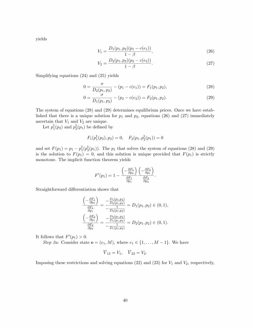
yields

V1 =D1(p1, p2)(p1 − c(e1))

1− β, (26)

V2 =D2(p1, p2)(p2 − c(e2))

1− β. (27)

Simplifying equations (24) and (25) yields

0 =σ

D2(p1, p2)− (p1 − c(e1)) = F1(p1, p2), (28)

0 =σ

D1(p1, p2)− (p2 − c(e2)) = F2(p1, p2). (29)

The system of equations (28) and (29) determines equilibrium prices. Once we have estab-lished that there is a unique solution for p1 and p2, equations (26) and (27) immediatelyascertain that V1 and V2 are unique.

Let p\1(p2) and p\

2(p1) be defined by

F1(p\1(p2), p2) = 0, F2(p1, p

\2(p1)) = 0

and set F (p1) = p1 − p\1(p

\2(p1)). The p1 that solves the system of equations (28) and (29)

is the solution to F (p1) = 0, and this solution is unique provided that F (p1) is strictlymonotone. The implicit function theorem yields

F ′(p1) = 1−

(−∂F1

∂p2

)

∂F1∂p1

(−∂F2

∂p1

)

∂F2∂p2

.

Straightforward differentiation shows that(−∂F1

∂p2

)

∂F1∂p1

=−D1(p1,p2)

D2(p1,p2)

− 1D2(p1,p2)

= D1(p1, p2) ∈ (0, 1),

(−∂F2

∂p1

)

∂F2∂p2

=−D2(p1,p2)

D1(p1,p2)

− 1D1(p1,p2)

= D2(p1, p2) ∈ (0, 1).

It follows that F ′(p1) > 0.Step 2a: Consider state e = (e1,M), where e1 ∈ {1, . . . , M − 1}. We have

V 12 = V1, V 22 = V2.

Imposing these restrictions and solving equations (22) and (23) for V1 and V2, respectively,

40

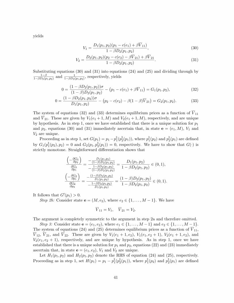
yields

V1 =D1(p1, p2)(p1 − c(e1) + βV 11)

1− βD2(p1, p2), (30)

V2 =D2(p1, p2)(p2 − c(e2)− βV 21) + βV 21

1− βD2(p1, p2). (31)

Substituting equations (30) and (31) into equations (24) and (25) and dividing through by1−β

1−βD2(p1,p2) and 11−βD2(p1,p2)

, respectively, yields

0 =(1− βD2(p1, p2))σ(1− β)D2(p1, p2)

− (p1 − c(e1) + βV 11

)= G1(p1, p2), (32)

0 =(1− βD2(p1, p2))σ

D1(p1, p2)− (

p2 − c(e2)− β(1− β)V 21

)= G2(p1, p2). (33)

The system of equations (32) and (33) determines equilibrium prices as a function of V 11

and V 21. These are given by V1(e1 + 1,M) and V2(e1 + 1,M), respectively, and are uniqueby hypothesis. As in step 1, once we have established that there is a unique solution for p1

and p2, equations (30) and (31) immediately ascertain that, in state e = (e1, M), V1 andV2 are unique.

Proceeding as in step 1, set G(p1) = p1−p\1(p

\2(p1)), where p\

1(p2) and p\2(p1) are defined

by G1(p\1(p2), p2) = 0 and G2(p1, p

\2(p1)) = 0, respectively. We have to show that G(·) is

strictly monotone. Straightforward differentiation shows that(−∂G1

∂p2

)

∂G1∂p1

=− D1(p1,p2)

(1−β)D2(p1,p2)

− 1−βD2(p1,p2)(1−β)D2(p1,p2)

=D1(p1, p2)

1− βD2(p1, p2)∈ (0, 1),

(−∂G2

∂p1

)

∂G2∂p2

=− (1−β)D2(p1,p2)

D1(p1,p2)

−1−βD2(p1,p2)D1(p1,p2)

=(1− β)D2(p1, p2)1− βD2(p1, p2)

∈ (0, 1).

It follows that G′(p1) > 0.Step 2b: Consider state e = (M, e2), where e2 ∈ {1, . . . ,M − 1}. We have

V 11 = V1, V 21 = V2.

The argument is completely symmetric to the argument in step 2a and therefore omitted.Step 3: Consider state e = (e1, e2), where e1 ∈ {1, . . . , M − 1} and e2 ∈ {1, . . . ,M − 1}.

The system of equations (24) and (25) determines equilibrium prices as a function of V 11,V 12, V 21, and V 22. These are given by V1(e1 + 1, e2), V1(e1, e2 + 1), V2(e1 + 1, e2), andV2(e1, e2 + 1), respectively, and are unique by hypothesis. As in step 1, once we haveestablished that there is a unique solution for p1 and p2, equations (22) and (23) immediatelyascertain that, in state e = (e1, e2), V1 and V2 are unique.

Let H1(p1, p2) and H2(p1, p2) denote the RHS of equation (24) and (25), respectively.Proceeding as in step 1, set H(p1) = p1 − p\

1(p\2(p1)), where p\

1(p2) and p\2(p1) are defined

41

by H1(p\1(p2), p2) = 0 and H2(p1, p

\2(p1)) = 0, respectively. We have to show that H(·) is

strictly monotone. Straightforward differentiation shows that(−∂H1

∂p2

)

∂H1∂p1

=−D1(p1,p2)

D2(p1,p2)

− 1D2(p1,p2)

= D1(p1, p2) ∈ (0, 1),

(−∂H2

∂p1

)

∂H2∂p2

=−D2(p1,p2)

D1(p1,p2)

− 1D1(p1,p2)

= D2(p1, p2) ∈ (0, 1).

It follows that H ′(p1) > 0.Case (ii): Next suppose δ = 1. A similar induction argument as in the case of δ = 0

can be used to establish the claim except that in the case of δ = 1 we anchor the argumentin state (1, 1) rather than state (M,M).

Proof of Proposition 5. Part (i): Consider the static Nash equilibrium. The FOCs instate e are

p†1(e) = c(e1) +σ

1−D1(p†1(e), p†2(e))

, (34)

p†2(e) = c(e2) +σ

1−D2(p†1(e), p†2(e))

. (35)

Equations (34) and (35) imply p†1(e) > c(e1) and p†2(e) > c(e2) and thus in particularp†(m, m) > c(m). In addition, p†(e) = p†(m,m) because c(e1) = c(e2) = c(m) for alle ∈ {m, . . . , M}2.

Turning to our dynamic stochastic game, suppose that δ = 0. The proof of part (i)proceeds in a number of steps, similar to the proof of Proposition 3. In step 1, we establishthat equilibrium prices in state (M, M) coincide with the static Nash equilibrium. In step2a, we assume that the equilibrium in state (e1+1,M), where e1 ∈ {m, . . . , M−1}, coincideswith the equilibrium in state (M, M) and show that this implies that the equilibrium instate (e1,M) does the same. In step 2b, we assume that the equilibrium in state (M, e2+1),where e2 ∈ {m, . . . ,M − 1}, coincides with the equilibrium in state (M, M) and show thatthis implies that the equilibrium in state (M, e2) does the same. In step 3, we assumethat the equilibrium in states (e1 + 1, e2) and (e1, e2 + 1), where e1 ∈ {m, . . . , M − 1} ande2 ∈ {m, . . . ,M − 1}, coincides with the equilibrium in state (M,M) and show that thisimplies that the equilibrium in state (e1, e2) does the same. Also similar to the proof ofProposition 3, we continue to use Vn as shorthand for Vn(e), V nk for V nk(e), pn for pn(e),etc.

Step 1: Consider state e = (M, M). From the proof of Proposition 3, equilibrium pricesare determined by the system of equations (28) and (29). Since equations (28) and (29)are equivalent to equations (34) and (35), equilibrium prices are p1 = p†1 and p2 = p†2.

42

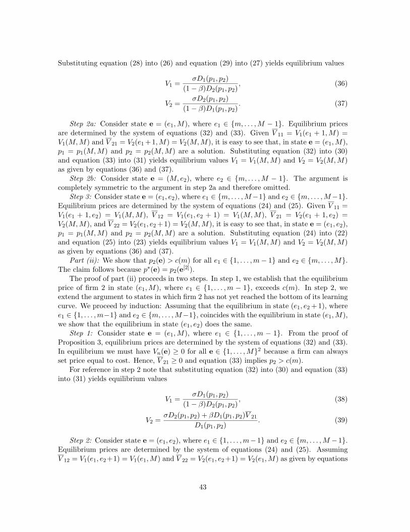
Substituting equation (28) into (26) and equation (29) into (27) yields equilibrium values

V1 =σD1(p1, p2)

(1− β)D2(p1, p2), (36)

V2 =σD2(p1, p2)

(1− β)D1(p1, p2). (37)

Step 2a: Consider state e = (e1, M), where e1 ∈ {m, . . . , M − 1}. Equilibrium pricesare determined by the system of equations (32) and (33). Given V 11 = V1(e1 + 1,M) =V1(M, M) and V 21 = V2(e1 +1,M) = V2(M, M), it is easy to see that, in state e = (e1,M),p1 = p1(M,M) and p2 = p2(M, M) are a solution. Substituting equation (32) into (30)and equation (33) into (31) yields equilibrium values V1 = V1(M, M) and V2 = V2(M,M)as given by equations (36) and (37).

Step 2b: Consider state e = (M, e2), where e2 ∈ {m, . . . , M − 1}. The argument iscompletely symmetric to the argument in step 2a and therefore omitted.

Step 3: Consider state e = (e1, e2), where e1 ∈ {m, . . . , M−1} and e2 ∈ {m, . . . ,M−1}.Equilibrium prices are determined by the system of equations (24) and (25). Given V 11 =V1(e1 + 1, e2) = V1(M,M), V 12 = V1(e1, e2 + 1) = V1(M, M), V 21 = V2(e1 + 1, e2) =V2(M, M), and V 22 = V2(e1, e2 +1) = V2(M,M), it is easy to see that, in state e = (e1, e2),p1 = p1(M,M) and p2 = p2(M, M) are a solution. Substituting equation (24) into (22)and equation (25) into (23) yields equilibrium values V1 = V1(M, M) and V2 = V2(M,M)as given by equations (36) and (37).

Part (ii): We show that p2(e) > c(m) for all e1 ∈ {1, . . . , m− 1} and e2 ∈ {m, . . . , M}.The claim follows because p∗(e) = p2(e[2]).

The proof of part (ii) proceeds in two steps. In step 1, we establish that the equilibriumprice of firm 2 in state (e1,M), where e1 ∈ {1, . . . , m − 1}, exceeds c(m). In step 2, weextend the argument to states in which firm 2 has not yet reached the bottom of its learningcurve. We proceed by induction: Assuming that the equilibrium in state (e1, e2 +1), wheree1 ∈ {1, . . . , m−1} and e2 ∈ {m, . . . ,M−1}, coincides with the equilibrium in state (e1,M),we show that the equilibrium in state (e1, e2) does the same.

Step 1: Consider state e = (e1, M), where e1 ∈ {1, . . . , m − 1}. From the proof ofProposition 3, equilibrium prices are determined by the system of equations (32) and (33).In equilibrium we must have Vn(e) ≥ 0 for all e ∈ {1, . . . , M}2 because a firm can alwaysset price equal to cost. Hence, V 21 ≥ 0 and equation (33) implies p2 > c(m).

For reference in step 2 note that substituting equation (32) into (30) and equation (33)into (31) yields equilibrium values

V1 =σD1(p1, p2)

(1− β)D2(p1, p2), (38)

V2 =σD2(p1, p2) + βD1(p1, p2)V 21

D1(p1, p2). (39)

Step 2: Consider state e = (e1, e2), where e1 ∈ {1, . . . ,m− 1} and e2 ∈ {m, . . . ,M − 1}.Equilibrium prices are determined by the system of equations (24) and (25). AssumingV 12 = V1(e1, e2+1) = V1(e1,M) and V 22 = V2(e1, e2+1) = V2(e1,M) as given by equations

43

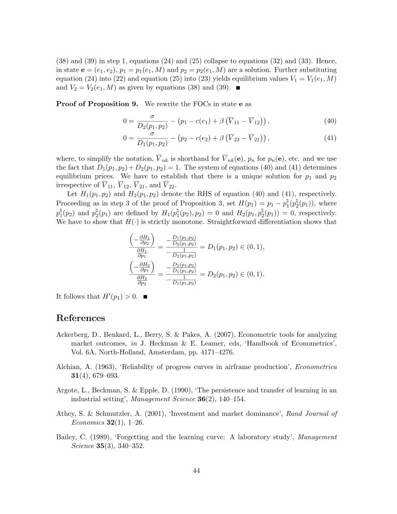
(38) and (39) in step 1, equations (24) and (25) collapse to equations (32) and (33). Hence,in state e = (e1, e2), p1 = p1(e1,M) and p2 = p2(e1, M) are a solution. Further substitutingequation (24) into (22) and equation (25) into (23) yields equilibrium values V1 = V1(e1,M)and V2 = V2(e1,M) as given by equations (38) and (39).

Proof of Proposition 9. We rewrite the FOCs in state e as

0 =σ

D2(p1, p2)− (

p1 − c(e1) + β(V 11 − V 12

)), (40)

0 =σ

D1(p1, p2)− (

p2 − c(e2) + β(V 22 − V 21

)), (41)

where, to simplify the notation, V nk is shorthand for V nk(e), pn for pn(e), etc. and we usethe fact that D1(p1, p2)+D2(p1, p2) = 1. The system of equations (40) and (41) determinesequilibrium prices. We have to establish that there is a unique solution for p1 and p2

irrespective of V 11, V 12, V 21, and V 22.Let H1(p1, p2) and H2(p1, p2) denote the RHS of equation (40) and (41), respectively.

Proceeding as in step 3 of the proof of Proposition 3, set H(p1) = p1 − p\1(p

\2(p1)), where

p\1(p2) and p\

2(p1) are defined by H1(p\1(p2), p2) = 0 and H2(p1, p

\2(p1)) = 0, respectively.

We have to show that H(·) is strictly monotone. Straightforward differentiation shows that(−∂H1

∂p2

)

∂H1∂p1

=−D1(p1,p2)

D2(p1,p2)

− 1D2(p1,p2)

= D1(p1, p2) ∈ (0, 1),

(−∂H2

∂p1

)

∂H2∂p2

=−D2(p1,p2)

D1(p1,p2)

− 1D1(p1,p2)

= D2(p1, p2) ∈ (0, 1).

It follows that H ′(p1) > 0.

References

Ackerberg, D., Benkard, L., Berry, S. & Pakes, A. (2007), Econometric tools for analyzingmarket outcomes, in J. Heckman & E. Leamer, eds, ‘Handbook of Econometrics’,Vol. 6A, North-Holland, Amsterdam, pp. 4171–4276.

Alchian, A. (1963), ‘Reliability of progress curves in airframe production’, Econometrica31(4), 679–693.

Argote, L., Beckman, S. & Epple, D. (1990), ‘The persistence and transfer of learning in anindustrial setting’, Management Science 36(2), 140–154.

Athey, S. & Schmutzler, A. (2001), ‘Investment and market dominance’, Rand Journal ofEconomics 32(1), 1–26.

Bailey, C. (1989), ‘Forgetting and the learning curve: A laboratory study’, ManagementScience 35(3), 340–352.

44

Baloff, N. (1971), ‘Extension of the learning curve: Some empirical results’, OperationalReserach Quarterly 22(4), 329–340.

Benkard, L. (2000), ‘Learning and forgetting: The dynamics of aircraft production’, Amer-ican Economic Review 90(4), 1034–1054.

Benkard, L. (2004), ‘A dynamic analysis of the market for wide-bodied commercial aircraft’,Review of Economic Studies 71(3), 581–611.

Berry, S. & Pakes, A. (2007), ‘The pure characteristics demand model’, International Eco-nomic Review 48(4), 1193–1225.

Bertsekas, D. & Tsitsiklis, J. (1997), Parallel and distributed computation: Numerical meth-ods, Athena Scientific, Belmont.

Bohn, R. (1995), ‘Noise and learning in semiconductor manufacturing’, Management Science41(1), 31–42.

Borkovsky, R., Doraszelski, U. & Kryukov, S. (2008), A user’s guide to solving dynamicstochastic games using the homotopy method, Working paper, Northwestern Univer-sity, Evanston.

Budd, C., Harris, C. & Vickers, J. (1993), ‘A model of the evolution of duopoly: Does theasymmetry between firms tend to increase or decrease?’, Review of Economic Studies60(3), 543–573.

Cabral, L. & Riordan, M. (1994), ‘The learning curve, market dominance, and predatorypricing’, Econometrica 62(5), 1115–1140.

Cabral, L. & Riordan, M. (1997), ‘The learning curve, predation, antitrust, and welfare’,Journal of Industrial Economics 45(2), 155–169.

Caplin, A. & Nalebuff, B. (1991), ‘Aggregation and imperfect competition: On the existenceof equilibrium’, Econometrica 59(1), 26–59.

Caves, R. & Porter, M. (1977), ‘From entry barriers to mobility barriers: Conjectural deci-sions and contrived deterrence to new competition’, Quarterly Journal of Economics91(2), 241–261.

Darr, E., Argote, L. & Epple, D. (1995), ‘The acquisition, transfer, and depreciation ofknowledge in service organizations: Productivity in franchises’, Management Science41(11), 1750–1762.

Dasgupta, P. & Stiglitz, J. (1988), ‘Learning-by-doing, market structure and industrial andtrade policies’, Oxford Economics Papers 40(2), 246–268.

DeJong, J. (1957), ‘The effects of increasing skills on cycle time and its consequences fortime standards’, Ergonomics 1(1), 51–60.

Demichelis, S. & Germano, F. (2002), ‘On (un)knots and dynamics in games’, Games andEconomic Behavior 41, 46–60.

45

Doraszelski, U. & Judd, K. (2008), Avoiding the curse of dimensionality in dynamic stochas-tic games, Working paper, Harvard University, Cambridge.

Doraszelski, U. & Satterthwaite, M. (2008), Computable Markov-perfect industry dynamics,Working paper, Harvard University, Cambridge.

Dudley, L. (1972), ‘Learning and productivity changes in metal products’, American Eco-nomic Review 62(4), 662–669.

Dutton, J. & Thomas, A. (1984), ‘Treating progress functions as a managerial opportunity’,Academy of Management Review 9(2), 235–247.

Ericson, R. & Pakes, A. (1995), ‘Markov-perfect industry dynamics: A framework for em-pirical work’, Review of Economic Studies 62, 53–82.

Friedman, J. (1971), ‘A non-cooperative equilibrium for supergames’, Review of EconomicStudies 38(1), 1–12.

Fudenberg, D. & Maskin, E. (1986), ‘The folk theorem in repeated games with discountingor with incomplete information’, Econometrica 54(3), 533–554.

Fudenberg, D. & Tirole, J. (1983), ‘Learning-by-doing and market performance’, Bell Jour-nal of Economics 14(2), 522–530.

Fudenberg, D. & Tirole, J. (1991), Game theory, MIT Press, Cambridge.

Garcia, C. & Zangwill, W. (1979), ‘An approach to homotopy and degree theory’, Mathe-matics of Operations Reserach 4(4), 390–405.

Ghemawat, P. & Spence, M. (1985), ‘Learning curve spillovers and market performance’,Quarterly Journal of Economics 100(Supplement), 839–852.

Grieco, P. (2008), Numerical approximation of an equilibrium correspondence: Method andapplications, Working paper, Northwestern University, Evanston.

Gruber, H. (1992), ‘The learning curve in the production of semiconductor memory chips’,Applied Economics 24, 885–895.

Hatch, N. & Mowery, D. (1998), ‘Process innovation and learning by doing in semiconductormanufacturing’, Management Science 44(1), 1461–1477.

Herings, J. & Peeters, R. (2004), ‘Stationary equilibria in stochastic games: Structure,selection, and computation’, Journal of Economic Theory 118, 32–60.

Hirschmann, W. (1964), ‘Profit from the learning curve’, Harvard Business Review42(1), 125–139.

Irwin, D. & Klenow, P. (1994), ‘Learning-by-doing spillovers in the seminconductor indus-try’, Journal of Political Economy 102(6), 1200–1227.

Jarmin, R. (1994), ‘Learning by doing and competition in the early rayon industry’, RandJournal of Economics 25(3), 441–454.

46

Judd, K. (1998), Numerical methods in economics, MIT Press, Cambridge.

Judd, K. & Schmedders, K. (2004), A computational approach to proving uniqueness indynamic games, Working paper, Hoover Institution, Stanford.

Kilbridge, M. (1962), ‘A model of industrial learning’, Management Science 8(4), 516–527.

Levy, F. (1965), ‘Adaptation in the production process’, Management Science 11(6), 136–154.

Lieberman, M. (1984), ‘The learning curve and pricing in the chemical processing industries’,Rand Journal of Economics 15(2), 213–228.

Maskin, E. & Tirole, J. (2001), ‘Markov perfect equilibrium, I: Observable actions’, Journalof Economic Theory 100, 191–219.

Pakes, A. (2008), Theorey and empirical work on imperfectly competitive markets, Fisher-Schultz lecture, Harvard University, Cambridge.

Pakes, A. & McGuire, P. (1994), ‘Computing Markov-perfect Nash equilibria: Numericalimplications of a dynamic differentiated product model’, Rand Journal of Economics25(4), 555–589.

Pisano, G. (1994), ‘Knowledge, integration, and the locus of learning: An empirical analysisof process development’, Strategic Management Journal 15, 85–100.

Preston, L. & Keachie, E. (1964), ‘Cost functions and progress functions: An integration’,American Economic Review 54(2), 100–107.

Ross, D. (1986), ‘Learning to dominate’, Journal of Industrial Economics 34(4), 337–353.

Rubinstein, A. (1979), ‘Equilibrium in supergames with the overtaking criterion’, Journalof Economic Theory 21(1), 1–9.

Schmedders, K. (1998), ‘Computing equilibria in the general equilibrium model with in-complete asset markets’, Journal of Economic Dynamics and Control 22, 1375–1401.

Schmedders, K. (1999), ‘A homotopy algorithm and an index theorem for the general equi-librium model with incomplete asset markets’, Journal of Mathematical Economics32(2), 225–241.

Shafer, S., Nembhard, D. & Uzumeri, M. (2001), ‘The effects of worker learning, forgetting,and heterogeneity on assembly line productivity’, Management Science 47(12), 1639–1653.

Shapley, L. (1953), ‘Stochastic games’, Proceedings of the National Academy of Sciences39, 1095–1100.

Spence, M. (1981), ‘The learning curve and competition’, Bell Journal of Economics12(1), 49–70.

47

Thompson, P. (2001), ‘How much did the Liberty shipbuilders learn? New evidence for anold case study’, Journal of Political Economy 109(1), 103–137.

Thompson, P. (2003), How much did the Liberty shipbuilders forget?, Working paper,Florida International University, Miami.

Thornton, R. & Thompson, P. (2001), ‘Learning from experience and learning from others:An exploration of learning and spillovers in wartime shipbuilding’, American EconomicReview 91(5), 1350–1368.

Vickers, J. (1986), ‘The evolution of market structure when there is a sequence of innova-tions’, Journal of Industrial Economics 35(1), 1–12.

Vives, X. (1999), Oligopoly pricing: Old ideas and new tools, MIT Press, Cambridge.

Watson, L., Billups, S. & Morgan, A. (1987), ‘HOMPACK: A suite of codes for glob-ally convergent homotopy algorithms’, ACM Transcations on Mathematical Software13(3), 281–310.

Watson, L., Sosonkina, M., Melville, R., Morgan, A. & Walker, H. (1997), ‘Algorithm777: HOMPACK90: A suite of Fortran 90 codes for globally convergent homotopyalgorithms’, ACM Transcations on Mathematical Software 23(4), 514–549.

Wixted, M. & Ebbesen, E. (1991), ‘On the form of forgetting’, Psychological Science2(6), 409–415.

Wright, T. (1936), ‘Factors affecting the cost of airplanes’, Journal of Aeronautical Sciences3(4), 122–128.

Zangwill, W. & Garcia, C. (1981), Pathways to solutions, fixed points, and equilibria, Pren-tice Hall, Englewood Cliffs.

Zimmerman, M. (1982), ‘Learning effects and the commercialization of new energy tech-nologies: The case of nuclear power’, Bell Journal of Economics 13(2), 297–310.

48

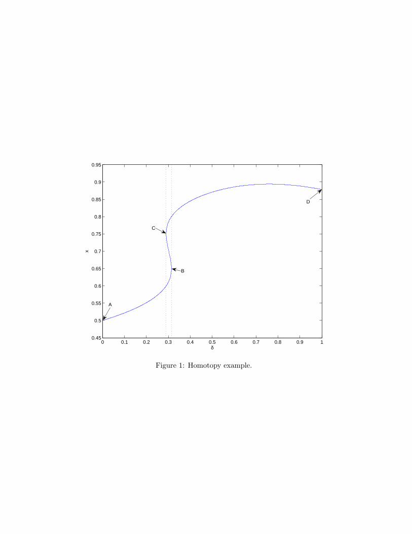
0 0.1 0.2 0.3 0.4 0.5 0.6 0.7 0.8 0.9 10.45

0.5

0.55

0.6

0.65

0.7

0.75

0.8

0.85

0.9

0.95

δ

x

A

B

C

D

Figure 1: Homotopy example.

0 0.01 0.03 0.05 0.1 0.2 1

0.1

0.2

0.3

0.4

0.5

0.6

0.7

0.8

0.9

1

δ

ρ

1

3

5

7

9

Figure 2: Number of equilibria.

0 0.03 0.1 0.3 10.5

0.51

0.55

0.7

1

δ

H∞

, H∧

ρ = 0.95

0 0.03 0.1 0.3 10.5

0.51

0.55

0.7

1

δ

H∞

, H∧

ρ = 0.75

0 0.03 0.1 0.3 10.5

0.51

0.55

0.7

1

δ

H∞

, H∧

ρ = 0.85

0 0.03 0.1 0.3 10.5

0.51

0.55

0.7

1

δ

H∞

, H∧

ρ = 0.65

0 0.03 0.1 0.3 10.5

0.51

0.55

0.7

1

δ

H∞

, H∧

ρ = 0.55

0 0.03 0.1 0.3 10.5

0.51

0.55

0.7

1

δ

H∞

, H∧

ρ = 0.15

0 0.03 0.1 0.3 10.5

0.51

0.55

0.7

1

δ

H∞

, H∧

ρ = 0.35

0 0.03 0.1 0.3 10.5

0.51

0.55

0.7

1

δ

H∞

, H∧

ρ = 0.05

Figure 3: Limiting expected Herfindahl index H∞ (solid line) and maximum expectedHerfindahl index H∧ (dashed line).

15

1015

2025

30

15

1015

2025

30

02468

1012

e1

Flat Eqbm. without Well (ρ=0.85, δ=0)

e2

p* (e1,e

2)

15

1015

2025

30

15

1015

2025

30

02468

1012

e1

Flat Eqbm. with Well (ρ=0.85, δ=0.0275)

e2

p* (e1,e

2)

15

1015

2025

30

15

1015

2025

30

02468

1012

e1

Trenchy Eqbm. (ρ=0.85, δ=0.0275)

e2

p* (e1,e

2)

15

1015

2025

30

15

1015

2025

30

02468

1012

e1

Extra−trenchy Eqbm. (ρ=0.85, δ=0.08)

e2

p* (e1,e

2)

Figure 4: Policy function p∗(e1, e2). Marginal cost c(e1) (solid line in e2 = 30-plane).

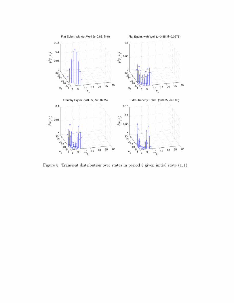
1 5 10 15 20 25 301

510

1520

2530

0

0.05

0.1

0.15

e1

Flat Eqbm. without Well (ρ=0.85, δ=0)

e2

µ8 (e1,e

2)

1 5 10 15 20 25 301

510

1520

2530

0

0.05

0.1

e1

Flat Eqbm. with Well (ρ=0.85, δ=0.0275)

e2

µ8 (e1,e

2)

1 5 10 15 20 25 301

510

1520

2530

0

0.05

0.1

e1

Trenchy Eqbm. (ρ=0.85, δ=0.0275)

e2

µ8 (e1,e

2)

1 5 10 15 20 25 301

510

1520

2530

0

0.05

0.1

0.15

e1

Extra−trenchy Eqbm. (ρ=0.85, δ=0.08)

e2

µ8 (e1,e

2)

Figure 5: Transient distribution over states in period 8 given initial state (1, 1).

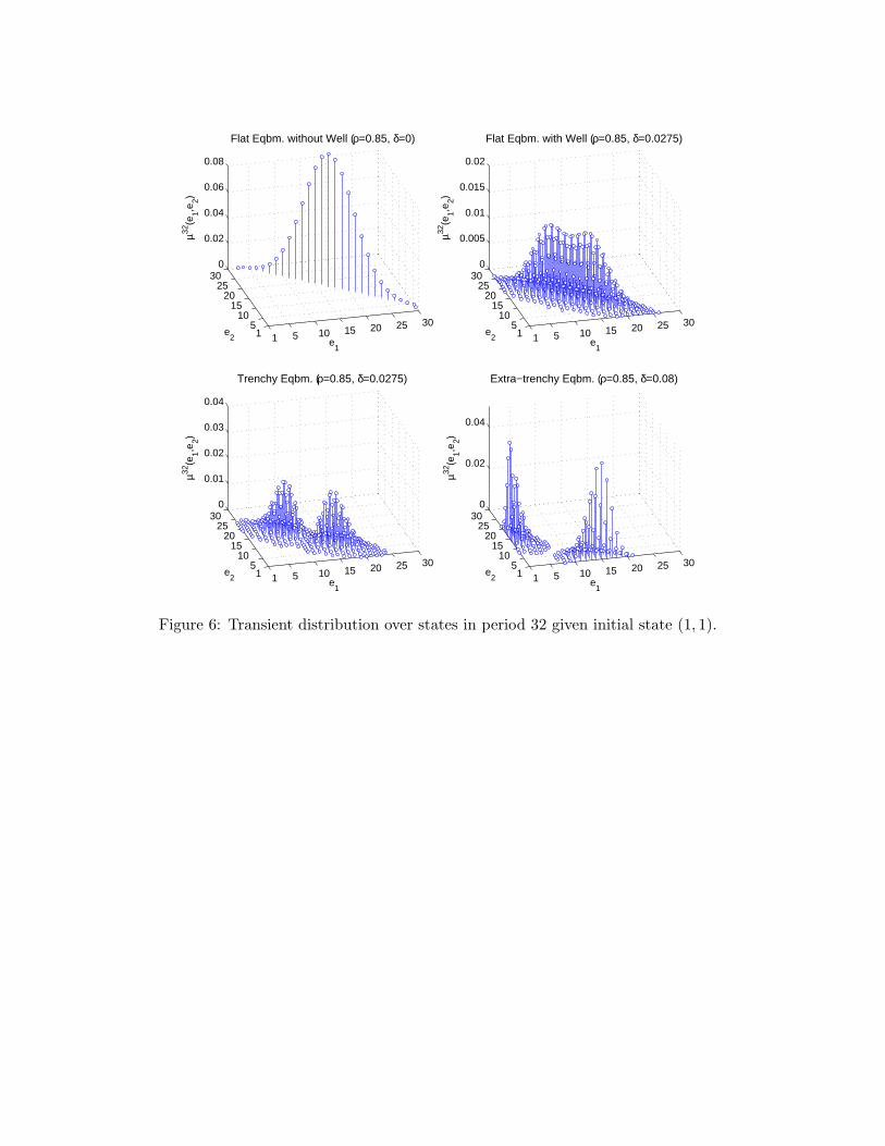
1 5 10 15 20 25 301

510

1520

2530

0

0.02

0.04

0.06

0.08

e1

Flat Eqbm. without Well (ρ=0.85, δ=0)

e2

µ32(e

1,e2)

1 5 10 15 20 25 301

510

1520

2530

0

0.005

0.01

0.015

0.02

e1

Flat Eqbm. with Well (ρ=0.85, δ=0.0275)

e2

µ32(e

1,e2)

1 5 10 15 20 25 301

510

1520

2530

0

0.01

0.02

0.03

0.04

e1

Trenchy Eqbm. (ρ=0.85, δ=0.0275)

e2

µ32(e

1,e2)

1 5 10 15 20 25 301

510

1520

2530

0

0.02

0.04

e1

Extra−trenchy Eqbm. (ρ=0.85, δ=0.08)

e2

µ32(e

1,e2)

Figure 6: Transient distribution over states in period 32 given initial state (1, 1).

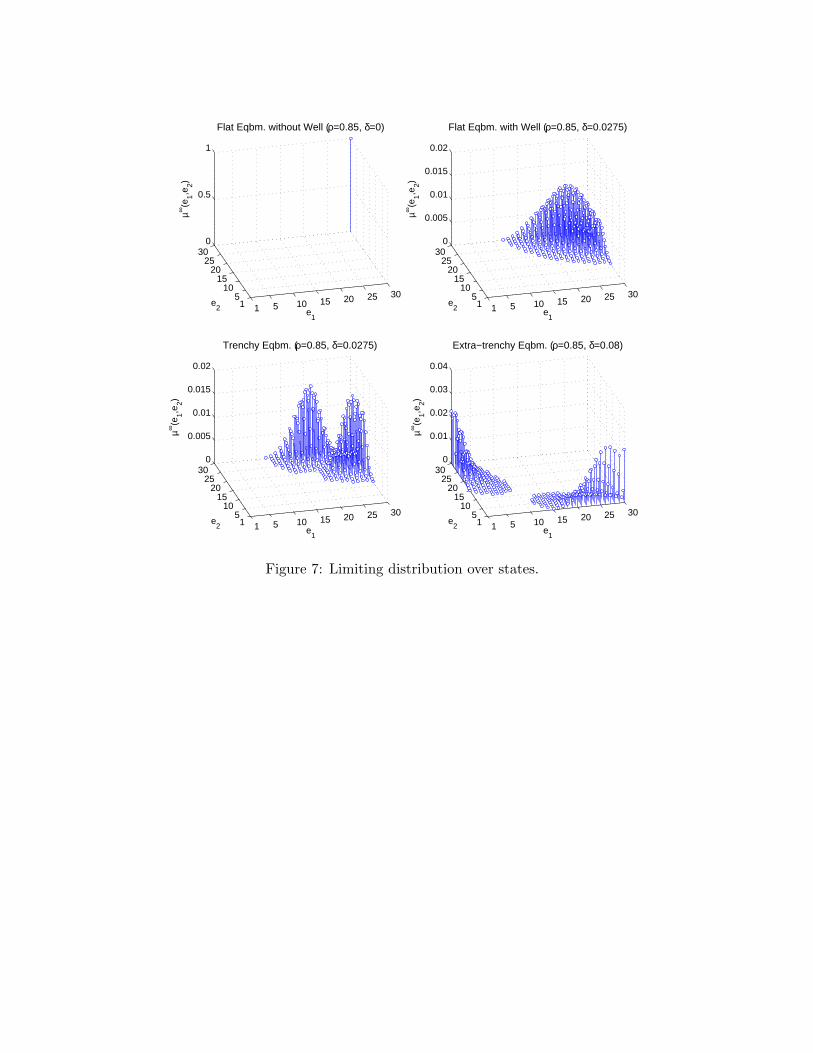
1 5 10 15 20 25 301

510

1520

2530

0

0.5

1

e1

Flat Eqbm. without Well (ρ=0.85, δ=0)

e2

µ∞(e

1,e2)

1 5 10 15 20 25 301

510

1520

2530

0

0.005

0.01

0.015

0.02

e1

Flat Eqbm. with Well (ρ=0.85, δ=0.0275)

e2

µ∞(e

1,e2)

1 5 10 15 20 25 301

510

1520

2530

0

0.005

0.01

0.015

0.02

e1

Trenchy Eqbm. (ρ=0.85, δ=0.0275)

e2

µ∞(e

1,e2)

1 5 10 15 20 25 301

510

1520

2530

0

0.01

0.02

0.03

0.04

e1

Extra−trenchy Eqbm. (ρ=0.85, δ=0.08)

e2

µ∞(e

1,e2)

Figure 7: Limiting distribution over states.

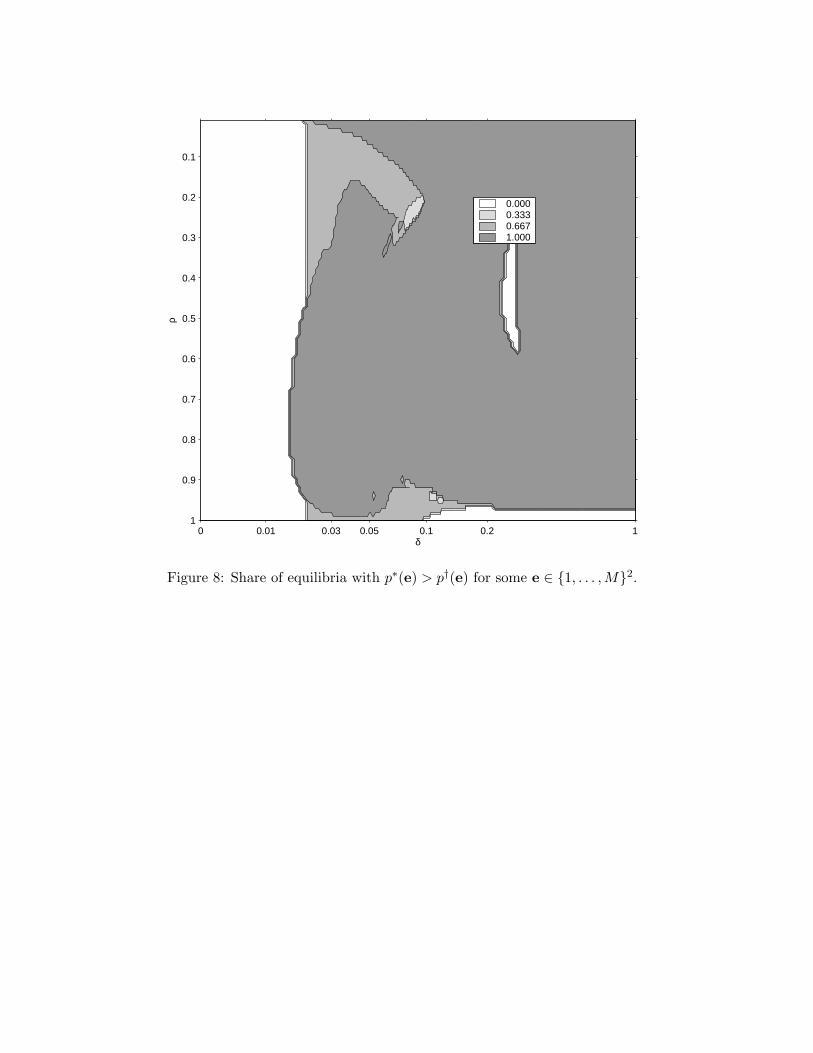
0 0.01 0.03 0.05 0.1 0.2 1

0.1

0.2

0.3

0.4

0.5

0.6

0.7

0.8

0.9

1

δ

ρ

0.000 0.333 0.667 1.000

Figure 8: Share of equilibria with p∗(e) > p†(e) for some e ∈ {1, . . . ,M}2.

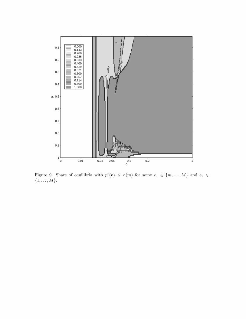
0 0.01 0.03 0.05 0.1 0.2 1

0.1

0.2

0.3

0.4

0.5

0.6

0.7

0.8

0.9

1

δ

ρ

0.000 0.143 0.200 0.286 0.333 0.400 0.429 0.571 0.600 0.667 0.714 0.800 1.000

Figure 9: Share of equilibria with p∗(e) ≤ c (m) for some e1 ∈ {m, . . . ,M} and e2 ∈{1, . . . , M}.

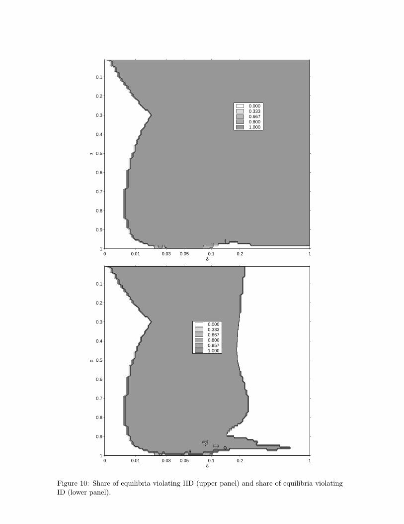
0 0.01 0.03 0.05 0.1 0.2 1

0.1

0.2

0.3

0.4

0.5

0.6

0.7

0.8

0.9

1

δ

ρ

0.000 0.333 0.667 0.800 1.000

0 0.01 0.03 0.05 0.1 0.2 1

0.1

0.2

0.3

0.4

0.5

0.6

0.7

0.8

0.9

1

δ

ρ

0.000 0.333 0.667 0.800 0.857 1.000

Figure 10: Share of equilibria violating IID (upper panel) and share of equilibria violatingID (lower panel).