Publications of the DLR elib

This is the author’s copy of the publication as archived with the DLR’s electronic library at

http://elib.dlr.de. Please consult the original publication for citation, see e.g.

https://www.springer.com/series/7393.

Learning-based Control for Hybrid Battery Management

Systems

J. Mirwald, R. de Castro, J. Brembeck, J. Ultsch and R. E. Araujo

Battery packs of electric vehicles are prone to capacity, thermal, and aging imbalances in their cells, which limit

power delivery to the vehicle. In this chapter, a hybrid battery management system (HBMS), capable of

simultaneously equalizing battery capacity and temperature while enabling hybridization with supercapacitors, is

investigated. We use model-free reinforcement learning to control the HBMS, where the control policy is obtained

through direct interaction with the system’s model. Our approach exploits the soft actor-critic algorithm to handle

continuous control actions and feedback states, and deep neural networks as function approximators. The

validation of the proposed control method is performed through numerical simulations, making use of numerically

efficient models of the energy storage and power converters developed in Modelica language.

Copyright Notice ©2020 Springer Nature Switzerland AG. Personal use of this material is permitted. Permission from Springer Nature Switzerland AG must be obtained for all other uses, in any current or future media, including reprinting/republishing this material for advertising or promotional purposes, creating new collective works, for resale or redistribution to servers or lists, or reuse of any copyrighted component of this work in other works.

This is a pre-print of the following chapter: J. Mirwald, R. de Castro, J. Brembeck, J. Ultsch and R. E. Araujo, “Learning-based Control for Hybrid Battery Management Systems”, published in Intelligent Control and Smart Energy Management: Renewable Resources and Transportation, Springer Optimization and Its Applications, edited by P. M. Pardalos, M. T. Thai, D. Du. Cham, Switzerland: Springer, 2021. Reproduced with permission of Springer Nature Switzerland AG. The final authenticated version is available online at: tbd.

Learning-based Control for Hybrid Battery Management Systems

Jonas Mirwald*, Ricardo de Castro*, Jonathan Brembeck*, Johannes Ultsch*, Rui Esteves Araujo **

*Institute of System Dynamics and Control, Robotics and Mechatronics Center, German Aerospace

Center (DLR), 82234 Weßling, Germany; firstname.lastname@dlr.de

**INESC TEC and Faculty of Engineering, University of Porto, Porto, 4200-465, Portugal

1. Abstract

Battery packs of electric vehicles are prone to capacity, thermal, and aging imbalances in their cells,

which limit power delivery to the vehicle. In this chapter, a hybrid battery management system (HBMS),

capable of simultaneously equalizing battery capacity and temperature while enabling hybridization

with supercapacitors, is investigated. We use model-free reinforcement learning to control the HBMS,

where the control policy is obtained through direct interaction with the system’s model. Our approach

exploits the soft actor-critic algorithm to handle continuous control actions and feedback states, and

deep neural networks as function approximators. The validation of the proposed control method is

performed through numerical simulations, making use of numerically efficient models of the energy

storage and power converters developed in Modelica language.

2. Introduction

Electric vehicles (EVs) are currently seen as a key technology for sustainable transportation. They

enable the integration of renewable energies with transportation systems and provide a promising

avenue to reduce environmental impact [1]. However, to fulfill these goals, several challenges need to

be addressed. One challenge is the parameter variations of large battery packs, which occurs due to

manufacturing tolerances and non-uniform aging of battery cells. These variations introduce the so-

called weakest-cell problem, i.e., the performance of the battery pack is limited by the cell with the

largest thermal and capacity degradation [2]. To overcome these issues, active balancing systems,

capable of equalizing charge and temperature, have been developed [3]. Another challenge in the design

of battery packs lies in the selection of battery chemistries which offer simultaneously high energy

density, high power density and long life. To attenuate these issues, hybrid and modular energy storage

systems, composed of heterogeneous units, have been investigated [4]. One promising research avenue

deals with battery-supercapacitor hybridization. Supercapacitors with high power density and durability

are particularly suited to handle rapid power bursts, while battery packs with high energy density can

provide average power during vehicle cruising. Numerous works have been utilizing these properties

to reduce peak power loads, weight and stress of the battery (see, e.g., [5] [6] and references therein).

Spurred by these balancing and hybridization challenges, a new class of battery balancing architecture,

called hybrid battery management system, was recently proposed by our group [7] (see Figure 1). The

HBMS is capable of simultaneously equalizing battery capacity and temperature while enabling

hybridization with additional storage systems, such as supercapacitors. Despite these attractive features,

the HBMS poses numerous control issues, such as coordinating a large number of power converters,

enforcing actuation and safety constraints and making trade-offs between multiple technical and

economic objectives. Model-based controllers, such as [7] [8], are one possible approach to tackle these

issues. These controllers rely on mathematical models that approximate and predict the behavior of the

plant (energy storage and power conversion in the HBMS). However, these models, usually obtained

from first principles, are not always easy to derive or parameterize. For example, batteries depend on

complex chemical reactions, requiring involved partial differential equations or complicated

approximations via electric-equivalent circuits [9], while power converters have switching and

nonlinear behavior [10]. Constructing and parameterizing these representations is time consuming,

subject to uncertainties and modelling mismatches, and often needs engineering insights to find a good

balance between complexity and accuracy. Additionally, the deployment of model-based controllers

needs, in some cases, significant computational effort, especially if optimization-based approaches are

used, which presents hurdles for execution in embedded systems.

Reinforcement learning (RL) offers an alternative design route to tackle some of these hurdles.

Similarly to optimal control, the RL algorithm tries to optimize a policy with regard to a predefined

reward function, encoding the control goal. In model-free RL this optimization is done solely based on

observed states, actions and rewards during the repeated interaction with the environment, called

training. One major advantage of using RL is the fact that simulation models (i.e., synthetic data) or

even the real plant can be used for the training process, avoiding the need for a controller synthesis

model. By using offline training against a simulation model, the computational effort is shifted to the

design stage, where significantly higher computational power is available. The obtained control policy,

usually a rather small multilayer neural network, can then be evaluated efficiently after deployment on

the target platform.

RL has been applied to a wide variety of problems, ranging from self-driving cars, to finance and

healthcare [11]. More recently, it has been considered for energy storage systems. For example, [12]

used RL to search for battery electrolyte compositions that can reduce electric conductivity. Energy

management of multiple energy storage systems (e.g. combining batteries, fuel-cells and/or

supercapacitors), is another task that plays to RL strengths. In this case, RL is well suited to handle the

stochastic uncertainties associated with future driving cycle information and to reduce computational

effort when compared to optimal receding control approaches [13] [14]. Energy storage arbitrage in

smart grids is another emerging problem tackled by RL. For example, [15] developed a Q-learning

based algorithms to decide when to buy energy from the grid, accumulate it in the battery and re-sell it

to the grid, while maximizing profit. In comparison with model-based solutions, these RL algorithms

were able to increase profit margins of grid operators by more than 50%. RL is also being applied to

derive control strategies for fast battery charging. For instance, [16] investigated the use of deep

deterministic policy gradient (DDPG) algorithms to reduce the charging times of batteries in the

presence of voltage and temperature constraints and parameter variations. One common element in

these previous works is the treatment of the battery at a pack-level, i.e., where capacity and temperature

variations of the modules/cells are neglected, and the battery operation is approximated by a single

virtual cell. To the best of the authors’ knowledge, the application of RL to control batteries at module-

or cell-level has received less attention in the literature to date (particularly in HBMS), which represents

a research gap that this work addresses.

The main contribution of this work consists in evaluating the potential of RL algorithms to control

HBMS. To support this investigation, we develop a numerical efficient simulation model of the HBMS

in Modelica language. Particular attention is dedicated to reducing numerical complexity of the HBMS

model, which is instrumental to decrease the training times of the RL algorithm - one of the main hurdles

when applying this method in practice. This efficient simulation model is then used to train a control

policy for the HBMS based on a soft actor-critic (SAC) algorithm [17] [18]. The application of SAC

algorithms brings two advantages: i) SAC is able to handle continuous control actions and feedback

states; ii) SAC offers a sample-efficient learning, thanks to its ability to automatically adapt exploration

control policies during training, often requiring less training time than other RL algorithms previously

employed in the control of energy storage systems, such as Q-learning [15] and DDPG [16].

RL

Training Algorithm

Battery 1

Supercapacitor PackPower

Converter 1

Load

Driving Cycle

Pload

Agent

Battery 2

…

Battery n

States

Action 1

…

iload

Action 2 Action n

Power

Converter 2

Power

Converter n

Figure 1: Block Diagram of the hybrid balancing system and the RL-based controller.

3. HBMS Modeling

3.1. Overview

As depicted in Figure 1, the HBMS is composed of a battery pack, supercapacitors (SCs), power

conversion and the load, which emulates the power consumption of the electric vehicle. The battery

pack contains n single-cell modules, connected in series. Each cell is linked with the primary side of a

bi-directional DC/DC power converter, while the converter’s secondary side is connected with SCs.

The power converters enable the cell-to-cell and the cell-to-SC transfer of energy. Our goal is to design

a RL-based control algorithm that uses the power converters to equalize charge and temperature, while

reducing current stress in the cells.

To support the design of the RL algorithm, we present in this section the modeling environment for the

HBMS. This modeling is carried out in Modelica, an object orientated, acausal and open source

language [19]. Modelica allows us to integrate different physical domains, such as electrical and

thermal, in the HBMS model. Its object-oriented features also enable us to automatize the creation of

multiple instances of battery cells and power converters. As a result, HBMS models with different

dimensions (ranging from a few cells to hundreds of cells) can be created with reduced coding effort.

Additionally, Modelica’s HBMS model can be exported through the functional mock-up interface

(FMI) standard [19] and combined with other simulation environments, such as Python [18], for training

RL agents.

3.2. Power Conversion

This sub-chapter presents the principle of operation and modelling of the power converter, with

particular emphasis on the efficient computation of energy losses.

3.2.1. Dual Half Bridge Converter

The power balancing hardware relies on a dual half bridge (DHB) configuration. In addition to galvanic

isolation, DHB offers zero-voltage switching, bidirectional power flow, and a reduced number of

switches when compared to dual full bridge configurations [20]. As depicted in Figure 2 the DHB

interfaces with the battery module (𝑣𝑏) on the primary side and with the SCs pack (𝑣sc) on the secondary

side. The DHB is composed of four main components: two input inductors (𝐿𝑏 , 𝐿sc), two half bridges

(𝑆1, 𝑆2 and 𝑆3, 𝑆4), auxiliary capacitors (𝐶1, … , 𝐶4) and a high-frequency transformer. The two half

bridges, and their four switches, regulate the power flow between primary and secondary sides of the

converter. This power is transferred via the high-frequency transformer and its leakage inductor (𝐿𝑠).

Through pulse-width modulation of the switches, two square voltage waveforms, shifted by 𝜙 [rad] and

with switching frequency 𝑓sw [1/s], are generated by the two half bridges and applied to the terminals

(𝑣𝑎𝑏 , 𝑣𝑐𝑑 in Figure 2)transformer. The resulting switching scheme is discussed in more detail at the

end of this section. The power extracted from the battery module is given by [21]:

𝑃(𝜙) = 𝑣𝑏𝑖𝑏 =𝜙(𝜋 − 𝜙)𝑣𝑏

2

𝜋 2𝜋𝑓sw 𝐿𝑠 (1)

which reveals that the maximum power flow is achieved when the phase shifts 𝜙 reaches 𝜋 2⁄ . To

further facilitate the control of power, we included an inner current loop in the DHB. This loop is based

on a proportional plus integrational control law and regulates the input current (𝑖𝑏) via manipulation of

the phase shift (𝜙). The interested reader is referred to [21] for additional details.

vb

S1

S2

v1

v2

C1

C2+

-

+

-Lb

ib

+

-

Ls

S3

S4

is

transformer C3

+

-

+

-

C4

battery side super capacitor side

+

-

vab

+

-

vcd

v3

v4

vsc+-

Lsc

isc

Figure 2: Schematic configuration of the dual half bridge.

We developed a detailed Modelica model of the DHB, incorporating energy losses. In Figure 3 (top)

the dual half bridge converter with a high frequency transformer is shown in a typical Modelica diagram

layer. All components are described in an a-causal representation with flow and potential variables

(i.e. voltage and current in case of electric systems – blue components). The red interfaces capture the

thermal flow between the components, and the magenta indicate Boolean control signals of the

switches. In Figure 3 (bottom) the sub-model of the half bridge, which is identical on both sides of the

DHB, is shown. The half-bridge model implements a DC-to-AC voltage conversion, and contains

copper and switching losses, as well parasitic elements, such as inductors’ resistances. The switches are

implemented through MOSFET transistors and an anti-parallel freewheeling diode, based on the

Infineon IPB009N03LG. The control strategy must prevent that the Boolean signals fire_p and fire_n

are true at the same time to avoid short circuits. Thanks to Modelica’s object-oriented design paradigm,

the DHB can be constructed using two instances of the half-bridges- see Figure 3 (top). The value of

the DHB parameters (𝐿𝑏 , 𝐿sc, 𝐶1, … , 𝐶4, etc) can be found in [21]- Table 5.3.

dual half bridge with high frequency transformer

half bridge model

S_1

_3

dio

_1

_3

S_2

_4

dio

_2

_4

C=

C_

B

C_

1_

3

C=

C_

B

C_

2_

4

L=LInOut

L_b_sc

R=R_Lio

R_L_b_sc

ac2

dc_p

dc_n

heatPort

ac

fire_

p

fire_

n

hB_bat_side

DC

AC

R

hB_SC_side

DC

AC

R

n=1

1 2

HFtransformer

L=Ls

L_s

R=R_2

R2

R=R_m

RmA

iB

V

Vab V

Vcd

bat_p SC_p

bat_n SC_n

heatPort

fire

_p1

fire

_n1

fire

_n2

fire

_p2

Figure 3: Modelica Model of the Dual Half Bridge Converter.

Figure 4 shows the simulation results of the DHB when operating with constant phase shift of 𝜙 =

0.3 ⋅ π/2 and voltages 𝑣b = 5.4 V, 𝑣SC = 4.5 V. The first plot shows the two MOSFET fire signals.

These signals are shifted by 𝜙 and generate square voltages (𝑣𝑎𝑏 , 𝑣𝑐𝑑) in the half-bridges (second plot).

The square voltages are applied to the transformer, leading to a large variation in the transformer’s

leakage inductor (third plot). The fourth plot shows the currents in the battery and SCs, which are

filtered by the DHB’s inductors. Finally, the last plot illustrates the power losses, which are discussed

in the detail in the next sub-section.

time [s]

false

true

[V]

0 [A]

0

8

[A]

0 +1E-5 +2E-5 +3E-5 +4E-5 +5E-5

0

2

[W] Ploss,C

0

S1,fire S3,fire

vab vcd

is

ib isc

Figure 4: Switching signals, voltages, currents and power losses of the DHB, obtained with phase shift of 𝜙 = 0.3 ⋅ 𝜋/2.

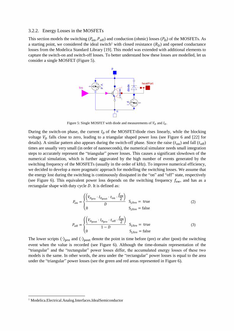
3.2.2. Energy Losses in the MOSFETs

This section models the switching (𝑃on, 𝑃off) and conduction (ohmic) losses (𝑃Ω) of the MOSFETs. As

a starting point, we considered the ideal switch1 with closed resistance (𝑅D) and opened conductance

losses from the Modelica Standard Library [19]. This model was extended with additional elements to

capture the switch-on and switch-off losses. To better understand how these losses are modelled, let us

consider a single MOSFET (Figure 5).

MO

SF

ET

dio

deV

V_d

Ai_d

fire

heatPort

p

n

Figure 5: Single MOSFET with diode and measurements of 𝑉𝐷 and 𝐼𝐷.

During the switch-on phase, the current 𝐼𝐷 of the MOSFET/diode rises linearly, while the blocking

voltage 𝑉𝐷 falls close to zero, leading to a triangular shaped power loss (see Figure 6 and [22] for

details). A similar pattern also appears during the switch-off phase. Since the raise (𝑡on) and fall (𝑡off)

times are usually very small (in order of nanoseconds), the numerical simulator needs small integration

steps to accurately represent the “triangular” power losses. This causes a significant slowdown of the

numerical simulation, which is further aggravated by the high number of events generated by the

switching frequency of the MOSFETs (usually in the order of kHz). To improve numerical efficiency,

we decided to develop a more pragmatic approach for modelling the switching losses. We assume that

the energy lost during the switching is continuously dissipated in the “on” and “off” state, respectively

(see Figure 6). This equivalent power loss depends on the switching frequency 𝑓sw, and has as a

rectangular shape with duty cycle 𝐷. It is defined as:

𝑃on = {(𝑉𝐷pre ⋅ 𝐼𝐷post ⋅ 𝑡on ⋅

𝑓sw2)

𝐷 Sj,fire = true

0 Sj,fire = false

(2)

𝑃off = {(𝑉𝐷post ⋅ 𝐼𝐷pre ⋅ 𝑡off ⋅

𝑓sw2)

1 − 𝐷 Sj,fire = true

0 Sj,fire = false

(3)

The lower scripts (∙)pre and (⋅)post denote the point in time before (pre) or after (post) the switching

event when the value is recorded (see Figure 6). Although the time-domain representation of the

“triangular” and the “rectangular” power losses differ, the accumulated energy losses of these two

models is the same. In other words, the area under the “rectangular” power losses is equal to the area

under the “triangular” power losses (see the green and red areas represented in Figure 6).

1 Modelica.Electrical.Analog.Interfaces.IdealSemiconductor

4e-5 5e-5 6e-5

0.00

0.04

0.06 [W

]

Pon Poff

false

true MOSFET

Fire

Pon PoffPpe ak

0.00

Qualitative

switch

losses

0.00

0.05

[W]

PΩ Ploss,M

Qualitatitve

blocking

voltage VD

vblock

0.00

Qualitative

current flow

ID

Ion

0.00

time [s]

𝑉𝐷post

𝐼𝐷pre

𝑉𝐷pre

𝐼𝐷post

𝑡on 𝑡off

0

Figure 6: Approximated MOSFET with switching and conduction (ohmic) losses.

Thanks to the “rectangular” approximation, we are able to avoid very small integration time steps that

would be necessary if the “triangular” power losses were modeled in detail. This brings an important

practical benefit: the simulation time of the HBMS can be reduced. The overall losses in the MOSFET

simulation model (𝑃loss,M) are therefore the sum of switching and conduction losses:

𝑃loss,M = 𝑃Ω + 𝑃on + 𝑃off (4)

where 𝑃Ω captures the Joule losses dissipated in the MOSFET resistance (𝑅D𝐼𝐷2).

3.2.3. Quasi-Stationary Model of the DHB

Despite the above simplifications, the simulation of the DHB model still generates a large number of

events. For example, for a test simulation run with constant voltage on the battery and SC sides and a

total simulation time of 5.7 s, the Modelica model of the DHB still needs a calculation time of about

421 s and generates ~1.3 ⋅ 106 events. This yields a poor real-time factor of 0.014 (DASSL2 solver,

Intel i7-8665U, 16 GB RAM, NVMe SSD).

To further reduce the simulation time, we decided to develop a quasi-stationary DHB model. This model

captures the main time constants of the DHB and calculates the energy losses and actuation limits

through multi-dimensional look-up tables. To parameterize these tables, we defined the following

operational range: i) voltage in the battery side, 𝑣b ∈ [2.7 V, 4.5 V], ii) voltage in the SC side 𝑣sc ∈[2.7 V, 5.4 V] and iii) phase shift 𝜙 ∈ [0, 𝜋 2⁄ ]. By means of parallelized parameter sweeping

simulations with an equidistant grid, all relevant data at the operations point could be generated. In

Figure 7 the resulting power losses for different operating points are shown; this allow us to build a

smooth multi-dimensional look-up table for the DHB power losses, 𝑃loss,C = 𝑓(𝑖b, 𝑣b, 𝑣SC), which

depends on the battery/SC voltage and input current (𝑖b). Note that 𝑃loss,C includes not only the

2 DASSL is a variable-order, variable-step numerical integration method

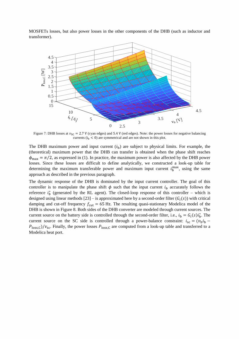
MOSFETs losses, but also power losses in the other components of the DHB (such as inductor and

transformer).

Plo

ss,C

[W

]

0

0.5

15

11.5

2

4.5

2.5

10

3

4

3.54

4.5

3.553

0 2.5

Figure 7: DHB losses at 𝑣SC = 2.7 V (cyan edges) and 5.4 V (red edges). Note: the power losses for negative balancing

currents (ib < 0) are symmetrical and are not shown in this plot.

The DHB maximum power and input current (𝑖b) are subject to physical limits. For example, the

(theoretical) maximum power that the DHB can transfer is obtained when the phase shift reaches

𝜙max = 𝜋 2⁄ , as expressed in (1). In practice, the maximum power is also affected by the DHB power

losses. Since these losses are difficult to define analytically, we constructed a look-up table for

determining the maximum transferable power and maximum input current 𝑖bmax, using the same

approach as described in the previous paragraph.

The dynamic response of the DHB is dominated by the input current controller. The goal of this

controller is to manipulate the phase shift 𝜙 such that the input current 𝑖𝑏 accurately follows the

reference 𝑖𝑏∗ (generated by the RL agent). The closed-loop response of this controller – which is

designed using linear methods [23] – is approximated here by a second-order filter (𝐺𝑖(𝑠)) with critical

damping and cut-off frequency 𝑓cut = 65 Hz. The resulting quasi-stationary Modelica model of the

DHB is shown in Figure 8. Both sides of the DHB converter are modeled through current sources. The

current source on the battery side is controlled through the second-order filter, i.e., 𝑖b = 𝐺𝑖(𝑠)𝑖b∗. The

current source on the SC side is controlled through a power-balance constraint: 𝑖sc = (𝑣b𝑖b −

𝑃loss,C)/𝑣sc. Finally, the power losses 𝑃loss,C are computed from a look-up table and transferred to a

Modelica heat port.

V

v_b

V

v_sci_

b

i_sc

DHB_dynamic

PTn

2

f=65 Hz

P_loss,C

u_1

u_n

y1_1

y1_n

...

...

TableND

i_b_max

i_b_lim

k=-1

i_sci_b

i_b_ref

bat_p

bat_n

SC_p

SC_n

heatPort

Figure 8: Quasi-stationary dual half bridge model in a mixed diagram and equation representation – Note: i_b_ref =𝑖b∗ .

The quasi-stationary DHB model provides a real-time factor of ~44.5, which is an improvement of

more then 3.2 ⋅ 105% when to compared to the switching DHB model presented in the previous section.

Figure 9 depicts the power losses obtained with the two modelling approaches using balancing currents

determined in [10]. The percentage goodness of fit (cf. [24] – C.5) of the power losses is about 84%,

which is an acceptable value considering the substantial improvement of the real-time simulation factor

obtained with the quasi-stationary DHB model. Because of these features, the quasi-stationary DHB

model was used in the training of the RL agent.

-1

0

1

2

3 [W] Switching Model (Ploss,C) Quasi-Stationary Model (Ploss,C)[A] ib

-10

-5

0

5

10

0 100 200 300 time [s]

Figure 9: Validation of the quasi-stationary DHB model.

3.3. Battery

This chapter discusses the battery model and its parameterization.

3.3.1. Battery Modeling

The battery model relies on the representation proposed in [25] and [26]. This model is modified to

better match the lithium nickel manganese cobalt oxide (NMC) chemistry (Li-Tec HEI40 40 Ah [27])

cell that is used in our group’s experimental vehicle, ROboMObil [28].

Ai

v_

int

V v_b

R

firstOrder

PT1

T=tau_d

IntegratorCurrent

I

k=1

beta_age

alpha_age

bat_p

bat_n

T

q

Figure 10: Implementation of the modified temperature-dependent generic battery model for NMC li-ion cells

(simplification) with age-defining parameters 𝛼age and 𝛽age.

Figure 10 shows the Modelica implementation of the battery cell. Each cell is composed of an internal

voltage source (𝑣int), equivalent series resistance (𝑅), and a Coulomb counter for the state-of-charge

(SoC). The internal cell’s voltage is calculated based on a combination of the following terms (see

Table 1):

• 𝑣0 captures linear temperature effects in the open-circuit voltage.

• (𝑣p,fs, 𝑣p,vs) are fixed/variable structure polarization voltages. The variable structure voltage

(𝑣p,vs) has switching dynamics, which is dependent on the filtered current 𝑖f and its sign. The

filtered current 𝑖f is calculated by applying a first-order filter to the cell current 𝑖 with a time

constant 𝜏d.

• 𝑣e captures the exponential voltage variations when the cell approaches full charging conditions

• 𝑣l1 is a linear voltage term, proportional to the battery charge 𝐼(𝑡) = 𝐼0 + ∫ 𝑖(𝑡)d𝑡, where 𝐼0 is

the initial charge.

• 𝑣l2 is an additional term that improves voltage course fitting to the NMC type cells used in this

work. This term provides a smooth transition to a second linear voltage term, which is activated

when the charge reaches the value 𝐼0. This transition is implemented through a logistic sigmoid

function 𝑓(𝑥) = logsig(𝑥) = 1/(1 + exp(−𝑥)) and its smoothness is adjusted via the

parameter 𝐼norm.

The equivalent series resistance 𝑅 (see Equation (14) in Table 1) has a nominal value 𝑅|𝑇a,ref,1, which

is obtained at a reference temperature 𝑇a,ref,1. This nominal value can be modified due to battery aging

factors (𝛼age) and Arrhenius-based temperature effects [9]. To compute the cell’s temperature, a heat

exchange model ( [24], Appendix C.2) is employed, which assumes that the heat transfer is dominated

by Joule losses in the series resistance, 𝑃loss,B = 𝑅(𝑇(𝑡)) ⋅ 𝑖2(𝑡). Finally, the cell’s capacity is

described by the variable 𝑄 (see (15) in Table 1), whose value can be reduced by the aging factor 𝛽𝑎𝑔𝑒.

The description of all the parameters employed in the battery model is presented in Table 2.

Table 1: Battery model equations

Description Equation Number

Internal cell’s voltage 𝑣int = 𝑣0 + 𝑣p,fs + 𝑣p,vs + 𝑣e + 𝑣l1 + 𝑣l2 (5)

Thermodynamics voltage 𝑣0 = 𝑣0|𝑇a,ref,1 +𝜕𝑣

𝜕𝑇⋅ (𝑇(𝑡) − 𝑇a,ref,1) (6)

Fixed-structure polarization

voltage 𝑣p,fs = −𝐾(𝑇(𝑡))𝐼(𝑡) ⋅

𝑄

𝑄 − 𝐼(𝑡) (7)

Variable-structure polarization

voltage 𝑣p,vs = (−

1

3600) ⋅ 𝐾(𝑇(𝑡)) 𝑖f(𝑡) ⋅ 𝑝𝑟(𝑄, 𝐼(𝑡), 𝑖f(𝑡)) (8)

Exponential zone voltage 𝑣e = 𝐴 ⋅ exp (−𝐵 ⋅ 𝐼(𝑡)) (9)

Linear zone 1 voltage 𝑣l1 = (−1) ⋅ 𝐶l,1 ⋅ 𝐼(𝑡) (10)

Linear zone 2 voltage 𝑣l2 = −𝐶l,2(𝐼(𝑡) − 𝐼1) ⋅ logsig (𝐼(𝑡) − 𝐼1𝐼norm

) (11)

Polarization constant 𝐾(𝑇(𝑡)) = 𝐾|𝑇a,ref,1 ⋅ exp (𝛼𝐾 ⋅ (1

𝑇(𝑡)−

1

𝑇a,ref,1)) (12)

Variable-structure polarization

ratio 𝑝𝑟 =

{

𝑄

𝜉𝑃𝑄 − 𝐼(𝑡), if 𝑖f(𝑡) ≥ 0

𝑄

𝜁𝑃𝑄 + 𝐼(𝑡), else

(13)

Resistance 𝑅 = (1 + 𝛼age) ⋅ 𝑅|𝑇a,ref,1 ⋅ exp (𝛽𝑅 ⋅ (1

𝑇(𝑡)−

1

𝑇a,ref,1)) (14)

Capacity 𝑄 = (1 − 𝛽age) ⋅ 𝑄|𝑇a,ref,1 (15)

State-of-charge 𝑞 = 1 −𝐼(𝑡)

𝑄 (16)

The computational efficiency provided by this battery model is high. For example, a dynamic single-

cell discharge simulation with a length of 1280 s, performed with a load as used during validation

(cf. Section 5.3), only takes about 0.5 s, yielding a real-time factor of 2560. Because of this fast

simulation time, no simplifications were performed in the battery model.

3.3.2. Battery Model Parametrization

The battery model was parameterized for NMC chemistry and used information from the cell’s

datasheet and experimental measurements [27]. The datasheet information allowed us to identify

parameters such as the nominal cell voltage. The experimental data was used to identify the remaining

parameters of the battery model through the following three-step optimization approach:

1. Experimental measurements from dynamic discharges (0°C and 25°C) were used to estimate

the temperature-related parameters (𝑅|𝑇a,ref,1, 𝛽𝑅). The squared temperature error was used as

cost function and minimized through the Simplex optimization algorithm [29].

2. Experimental measurements from the constant-current charge/discharge references (0°C and

25°C) were used to estimate the parameters that affect the internal voltage (such as 𝜕𝑣

𝜕𝑇, 𝐾|𝑇a,ref,1,

𝛼𝐾, 𝐶l,1, 𝑄|𝑇a,ref,1, 𝐶l,2, 𝐼1 and 𝐼norm). The squared voltage error was used as cost function and

minimized through a genetic algorithm [29].

3. The parameters obtained in step 2 were then used as initial values for a second optimization run

using the Simplex algorithm, allowing us to further refine the parameter estimate.

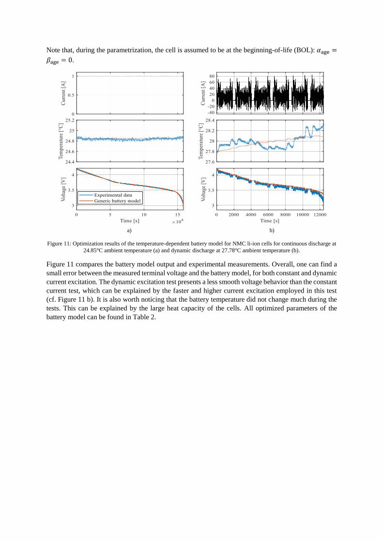
Note that, during the parametrization, the cell is assumed to be at the beginning-of-life (BOL): 𝛼age =

𝛽age = 0.

a) b)

Figure 11: Optimization results of the temperature-dependent battery model for NMC li-ion cells for continuous discharge at

24.85°C ambient temperature (a) and dynamic discharge at 27.78°C ambient temperature (b).

Figure 11 compares the battery model output and experimental measurements. Overall, one can find a

small error between the measured terminal voltage and the battery model, for both constant and dynamic

current excitation. The dynamic excitation test presents a less smooth voltage behavior than the constant

current test, which can be explained by the faster and higher current excitation employed in this test

(cf. Figure 11 b). It is also worth noticing that the battery temperature did not change much during the

tests. This can be explained by the large heat capacity of the cells. All optimized parameters of the

battery model can be found in Table 2.

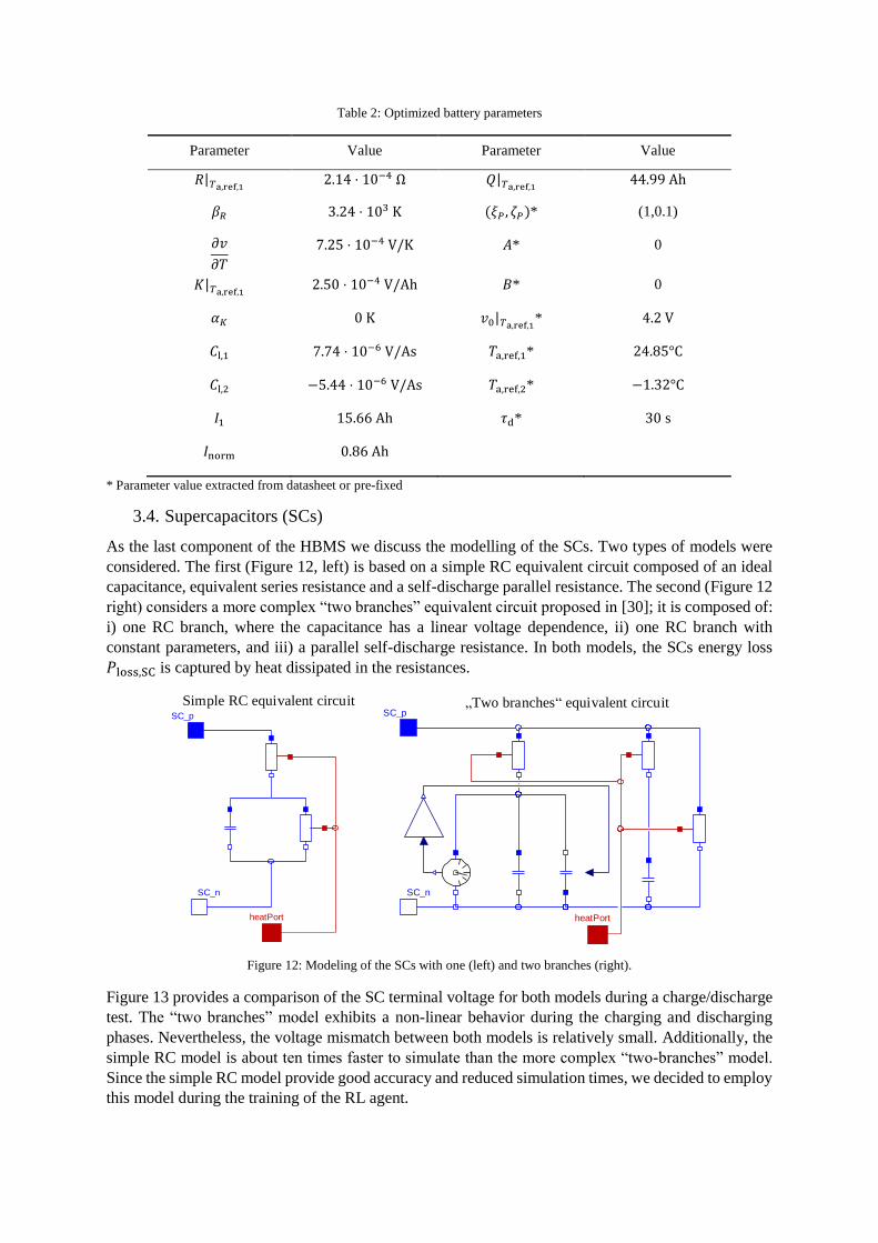
Table 2: Optimized battery parameters

Parameter Value Parameter Value

𝑅|𝑇a,ref,1 2.14 ⋅ 10−4 Ω 𝑄|𝑇a,ref,1 44.99 Ah

𝛽𝑅 3.24 ⋅ 103 K (𝜉𝑃 , 𝜁𝑃)* (1,0.1)

𝜕𝑣

𝜕𝑇

7.25 ⋅ 10−4 V/K 𝐴* 0

𝐾|𝑇a,ref,1 2.50 ⋅ 10−4 V/Ah 𝐵* 0

𝛼𝐾 0 K 𝑣0|𝑇a,ref,1* 4.2 V

𝐶l,1 7.74 ⋅ 10−6 V/As 𝑇a,ref,1* 24.85°C

𝐶l,2 −5.44 ⋅ 10−6 V/As 𝑇a,ref,2* −1.32°C

𝐼1 15.66 Ah 𝜏d* 30 s

𝐼norm 0.86 Ah

* Parameter value extracted from datasheet or pre-fixed

3.4. Supercapacitors (SCs)

As the last component of the HBMS we discuss the modelling of the SCs. Two types of models were

considered. The first (Figure 12, left) is based on a simple RC equivalent circuit composed of an ideal

capacitance, equivalent series resistance and a self-discharge parallel resistance. The second (Figure 12

right) considers a more complex “two branches” equivalent circuit proposed in [30]; it is composed of:

i) one RC branch, where the capacitance has a linear voltage dependence, ii) one RC branch with

constant parameters, and iii) a parallel self-discharge resistance. In both models, the SCs energy loss

𝑃loss,SC is captured by heat dissipated in the resistances.

Simple RC equivalent circuit Two branches equivalent circuit

heatPort

SC_p

SC_n

heatPort

SC_p

SC_n

Figure 12: Modeling of the SCs with one (left) and two branches (right).

Figure 13 provides a comparison of the SC terminal voltage for both models during a charge/discharge

test. The “two branches” model exhibits a non-linear behavior during the charging and discharging

phases. Nevertheless, the voltage mismatch between both models is relatively small. Additionally, the

simple RC model is about ten times faster to simulate than the more complex “two-branches” model.

Since the simple RC model provide good accuracy and reduced simulation times, we decided to employ

this model during the training of the RL agent.

0 25 50 75 100 125 150 0.0

0.5

1.0

1.5

2.0

2.5

3.0 [V] RC model Two Branches

-30

-20

-10

0

10

20

30 [A] isc

Figure 13: Comparison of the modeling with one or two branches (parameters extracted from [30]).

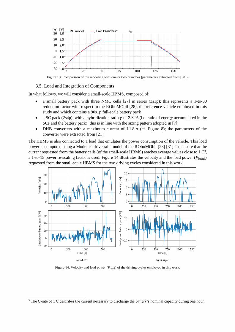
3.5. Load and Integration of Components

In what follows, we will consider a small-scale HBMS, composed of:

• a small battery pack with three NMC cells [27] in series (3s1p); this represents a 1-to-30

reduction factor with respect to the ROboMObil [28], the reference vehicle employed in this

study and which contains a 90s1p full-scale battery pack

• a SC pack (2s4p), with a hybridization ratio 𝛾 of 2.3 % (i.e. ratio of energy accumulated in the

SCs and the battery pack); this is in line with the sizing pattern adopted in [7]

• DHB converters with a maximum current of 11.8 A (cf. Figure 8); the parameters of the

converter were extracted from [21].

The HBMS is also connected to a load that emulates the power consumption of the vehicle. This load

power is computed using a Modelica drivetrain model of the ROboMObil [28] [31]. To ensure that the

current requested from the battery cells (of the small-scale HBMS) reaches average values close to 1 C3,

a 1-to-15 power re-scaling factor is used. Figure 14 illustrates the velocity and the load power (𝑃load)

requested from the small-scale HBMS for the two driving cycles considered in this work.

a) WLTC b) Stuttgart

Figure 14: Velocity and load power (𝑃load) of the driving cycles employed in this work.

3 The C-rate of 1 C describes the current necessary to discharge the battery’s nominal capacity during one hour.

4. Reinforcement Learning

This section presents the principle of operation of the selected reinforcement learning algorithm of this

work as well as its application to the HBMS.

4.1. Principle of Operation

RL algorithms are developed assuming a stochastic environment, usually formulated as a Markov

decision process (MDP). At time step 𝑘, the MDP receives an action 𝒂𝑘 ∈ 𝒜 ⊂ ℝ𝑚 and produces a

state vector 𝒔𝑘 ∈ 𝒮 ⊂ ℝ𝑛, where 𝒜 and 𝒮 are the action and state spaces, respectively. The state evolves

according to state-transition probability 𝑝(𝒔𝑘+1|𝒔𝑘, 𝒂𝑘), which denotes the probability of transitioning

from state 𝒔𝑘 to state 𝒔𝑘+1 by taking the action 𝒂𝑘 [32]. After the transition to state 𝒔𝑘+1, the reward

𝑟𝑘+1 is assigned. This interaction, as depicted in Figure 15, leads to a trajectory

𝒔𝑘 , 𝒂𝑘 , 𝑟𝑘+1, 𝒔𝑘+1, 𝒂𝑘+1, 𝑟𝑘+2, …. A trajectory is called an episode, if a terminal state is reached and a

reset to initial conditions occurs. The sum of rewards of an episode is referred to as the return.

Environment

Action ak

State sk

Reward rk

1s 1p

ground

1s 1p

1s 1p

u_1u_n

y1_1y1_n.. .

.. .

DC

DC

u_1u_n

y1_1y1_n.. .

.. .

DC

DC

u_1u_n

y1_1y1_n.. .

.. .

DC

DC

hcD

CD

C

hcB

at

i_load

i_b_1

i_b_2

i_b_3

litec_HEI40_1

litec_HEI40_2

exte

rna

lLoa

d

DHB_1

DHB_2

DHB_3litec_HEI40_3

hcS

C

1s 4p

1s 4p

Agent

Figure 15: Interaction of reinforcement learning agent with environment [32].

The RL goal is to find an optimal policy 𝜋∗(𝒂𝑘|𝒔𝑘) that maximizes the expected return 𝐽

𝐽 =∑𝔼(𝒔𝑘,𝒂𝑘)~𝜌 𝜋𝑘

[𝑟(𝒔𝑘, 𝒂𝑘)] (17)

with the expectation denoted by 𝔼 and 𝜌𝜋(𝒔𝑘 , 𝒂𝑘) being the state-action marginal of the trajectory

distribution induced by the stochastic policy 𝜋(𝒂𝑘|𝒔𝑘) (cf. [17]). While trying to optimize the policy

(exploitation) based on the observed transition trajectories, a certain randomness during the training is

necessary to discover the full state and action space (exploration). Several types of RL algorithms can

be used to minimize 𝐽. In the Soft Actor-Critic algorithm [17], which is adopted in this work, the

standard RL objective (17) is augmented with an information-theoretical entropy term ℋ(𝑋) (cf. [33]):

�̃� =∑𝔼(𝒔𝑘,𝒂𝑘)~𝜌 𝜋𝑘

[𝑟(𝒔𝑘, 𝒂𝑘) + 𝛼ℋ(𝜋(⋅ |𝒔𝑘))] (18)

where 𝛼 represents a weight (known as temperature parameter), which allows us to balance exploration

and exploitation. By starting the training with a high value of 𝛼, higher levels of exploration and

discovery can be promoted. Afterwards, as the agent learns the impact of its actions in the environment

and rewards, lower values of 𝛼 can be deployed, shifting the focus toward exploitation [34]. Previous

research has shown that the SAC algorithm offers a sample-efficient learning and outperforms other

widely-used RL algorithms [34].

The SAC algorithm [34] is an off-policy actor-critic algorithm incorporating a replay buffer and neural

networks to approximate the policy (actor) as well as two action-value functions (critic). The action-

value functions are used to account for positive bias in the policy improvement step which can

deteriorate performance (cf. [35], [36]). Moreover, two additional target neural networks are used to

stabilize training. In the SAC algorithm, the stochastic policy is usually parametrized as a gaussian with

mean and variance given by the actor neural network. During training, the SAC alternates between

performing environment steps and gradient steps. To perform an environment step, an action is sampled

out of the gaussian policy and applied to the environment. Together with the returned reward and next

state, the sampled action is then stored inside the replay buffer. During the gradient step phase the

parameters of the policy, the two action-value functions and the temperature parameter are updated with

stochastic gradient descent steps, which are computed based on uniformly sampled batches of the replay

buffer. As a last step during the gradient step phase, the target networks’ parameters are computed as

an exponentially moving average of the parameters of the two action-value functions. The environment

step phase and the gradient step phase are repeated until a certain amount of iterations is reached [35],

[36]. After training the deterministic part of the policy is used for deployment.

4.2. Application of Deep Reinforcement Learning to the HBMS

To apply the RL to the HBMS, we need to specify: i) the actions (𝒂𝑘); ii) the state vector (𝒔𝑘) and iii)

the reward function (𝑟𝑘 ) that contains the control objectives.

4.2.1. Actions

The RL actions 𝒂𝑘 consist of the reference currents 𝑖b,𝑘,𝑗∗ for each 𝑗-th power converter:

𝒂𝑘 = [𝑖b,𝑘,1∗ , … , 𝑖b,𝑘,𝑛

∗ ]T. (19)

The actions are subject to saturation and rate limit constraints. As discussed in Section 3.2.3, the DHB

saturates the maximum current 𝑖b,𝑘,𝑗max(𝑞SC,𝑘 , 𝑞𝑘,𝑗) that can be extracted from each battery cell. This

saturation is modelled here as:

𝑎𝑘,𝑗sat = {

𝑎𝑘,𝑗 , if |𝑎𝑘,𝑗| ≤ 𝜂𝑎 ⋅ 𝑎max,𝑘𝜂𝑎 ⋅ 𝑎max,𝑘, if 𝑎𝑘,𝑗 ≥ 𝜂𝑎 ⋅ 𝑎max,𝑘

−𝜂𝑎 ⋅ 𝑎max,𝑘, if 𝑎𝑘,𝑗 ≤ −𝜂𝑎 ⋅ 𝑎max,𝑘

, 𝑎max,𝑘 = min𝑗𝑖b,𝑘,𝑗max(𝑞SC,𝑘, 𝑞𝑘,𝑗) (20)

where 𝑎𝑘,𝑗sat is the saturated action for the 𝑗-th power converter, 𝑎max,𝑘 the worst-case current limit

among all power converters, and 𝜂𝑎 = 0.9 a safety margin.

The action is rate limited as a means to enforce smoothness of the RL actions. It is defined as:

Δ𝑎𝑘,𝑗𝑠𝑎𝑡 = |𝑎𝑘,𝑗 − 𝑎𝑘−1,𝑗

sat | ≤ Δ𝑎max ⋅ Δ𝑡 . (21)

where 𝑎𝑘−1,𝑗sat is the action applied in the previous time step, Δ𝑎max = 2.5 A/s the current rate limit

(defined by the control engineer) and Δ𝑡 = 1 s the sample time.

4.2.2. State Vector

The state vector 𝒔𝑘 is defined as follows:

𝒔𝑘 = [𝒒𝑘T, 𝑞SC,𝑘, Δ𝒒𝑘

T, Δ𝑻𝑘T, 𝒂𝑘−1

sat T, 𝑎max,𝑘, 𝜶ageT , 𝜷age

T , 𝑖load,𝑘]T. (22)

where

• 𝒒𝑘 = [𝑞𝑘,1 , … , 𝑞𝑘,𝑛]T

and 𝑞SC,𝑘 represent the SoC of the battery cells and SC pack

• Δ𝑞𝑘,𝑗 and Δ𝑇𝑘,𝑗 represent the SoC and temperature deviations, computed as:

Δ𝒒𝑘 = [Δ𝑞𝑘,1, … , Δ𝑞𝑘,𝑛]T, Δ𝑞𝑘,𝑗 = 𝑞𝑘,𝑗 − �̅�𝑘 (23)

Δ𝑻𝑘 = [Δ𝑇𝑘,1, … , Δ𝑇𝑘,𝑛]T, Δ𝑇𝑘,𝑗 = 𝑇𝑘,𝑗 − �̅�𝑘 (24)

where �̅� and �̅� correspond to the mean SoC and mean temperature of the battery pack,

respectively.

• 𝒂𝑘−1sat and 𝑎max,𝑘 are the actions applied in the previous time step and the saturation limits,

respectively. This information helps the RL agent to enforce rate and range limits.

• 𝜶age = [𝛼age,1, … , 𝛼age,n]T

and 𝜷age = [𝛽age,1, … , 𝛽age,n]T

contain information about the

variability of the cell’s inner resistance and capacity. This information can be obtained by

battery diagnosis algorithms (such as [9]) and it helps the RL agent to understand the cell-to-

cell variability in the battery pack.

• 𝑖load,𝑘 represents the load current requested from the battery pack. It is computed based on the

battery voltage and load power (𝑃load) requested from the battery pack (see Section 3.5)

It is worth noticing that the above states are normalized with respect to their maximum expected values

before passing them to the RL agent.

4.2.3. Reward Function

The goal of the RL is to minimize: i) battery current stress, ii) SoC deviations Δ𝒒, iii) temperature

deviations Δ𝑻, and iv) power losses, v) while maintaining smooth control values 𝒂. For this, the

following nominal reward function is used:

𝑟no abort,𝑘 = −1

𝑤𝑖2 ⋅∑(1 + 𝛼age,𝑗) ⋅ 𝑖𝑘,𝑗

2

n

𝑗=1

−1

𝑤Δ𝑇2 ⋅ Δ𝑻𝑘

TΔ𝑻𝑘 −1

𝑤Δ𝑞2 ⋅ Δ𝒒𝑘

TΔ𝒒𝑘

−1

𝑤𝑙⋅ 𝑃losses,𝑘 −

1

𝑤Δ𝑎⋅ ∑|Δ𝑎𝑘,𝑗

sat|

n

𝑗=1

(25)

where 𝑤𝑖, 𝑤ΔT, 𝑤Δ𝑞 , 𝑤Δ𝑎 are weights that the designer can use to prioritize different control goals and

normalize the different reward terms.

The first term of the reward function aims at the reduction of the module current 𝑖𝑘,𝑗 = 𝑎𝑘,𝑗sat + 𝑖load,𝑘;

it encourages the use of battery modules with less degradation, i.e. with lower aging factor 𝛼age,𝑗. The

following two terms aim at the reduction of temperature and SoC deviations, respectively. The fourth

term enables the learning of smooth actions 𝒂 by penalizing large differences between the current (𝒂𝑘)

and the previously action (𝒂𝑘−1sat ). Finally, the last term aims at the reduction of the power losses in the

battery modules, converters and SCs:

𝑃losses =∑(𝑃loss,B,j + 𝑃loss,C,j + 𝑃loss,SC,j)

n

𝑗=1

(26)

There are several conditions that might prematurely end an episode, in which case the (highly) negative

reward 𝑟abort < 0 is assigned at that time step 𝑘 instead of 𝑟no abort,𝑘. This abort mechanism speeds up

the training by showing the agent that specific state-action pairs are less desirable. The final reward

function is therefore described as:

𝑟 𝑘 = {𝑟no abort,𝑘 , if 𝑎𝑏𝑜𝑟𝑡𝑘 = false

𝑟abort, else (27)

where 𝑎𝑏𝑜𝑟𝑡𝑘 is a Boolean condition that becomes true when the following state constraints are

violated:

50 % ≤ 𝑞SC,𝑘 ≤ 100 %, 5 % ≤ 𝑞𝑘,𝑗 ≤ 95 %. (28)

These constraints prevent deep discharge and overcharge of the battery cells and SCs and must be

enforced by the RL agent.

5. Results and Discussion

This section presents the training setup, training results and validation results obtained when controlling

the HBMS with the RL algorithm.

5.1. Training Setup

To train the RL agent, the control engineer needs to specify several parameters, including the training

length, the initial values of the HBMS model, the SAC parameters and the weights of the reward

function.

Regarding the training length: each episode has a maximum length of 500 s (representing 500 time

steps), which is sufficiently large to cover the dominant time constants of the HBMS. The overall

training process consists of 2 ⋅ 106 time steps, which is also adequately long to achieve convergence

for the reward functions.

The initial values of the parameters of the environment (the HBMS model) are randomized in order to

increase the robustness of the RL agent; this also decreases overfitting to a specific system initialization.

The initial values are sampled from a continuous uniform distribution with intervals summarized in

Table 3. These parameters include, for example, the initial time of the driving cycle (𝑡dc,0), which allows

the RL agent to be exposed to a different sequence of load current 𝑖load,𝑘 during the episodes.

Miscellaneous values for the initial SoC aging are also considered. For the aging factors, we assume

that 𝛼age,𝑗 and 𝛽age,𝑗 are fully correlated for a single module (e.g., when 𝛼age,𝑗 = 0 we also have

𝛽age,𝑗 = 0), while there is no correlation assumed between modules.

Table 3: Random sampling for training initialization

Description Variable Sampling interval

Beginning of driving cycle* 𝑡dc,0 [0 s, 1299 s]

Module’s initial temperature** 𝑇0,𝑗 [𝑇a − 1°𝐶, 𝑇a + 1 °𝐶]

Initial mean of the modules’ SoC �̅�0 [45 %, 85 %]

Initial module’s deviation from the

sampled mean Δ𝑞0,𝑗 [−5 %, 5 %]

Fixed resistance increase*** 𝛼age,𝑗 [0, 𝛼age,EOL]

Fixed capacity decrease*** 𝛽age,𝑗 [0, 𝛽age,EOL]

Supercapacitor pack’s SoC 𝑞SC,0 [75 %, 95%]

* the WLTC driving cycle is used during training of the RL agent

** ambient temperature: 𝑇a = 25 °C

*** end-of-life (EOL) values: 𝛼age,EOL = 240 % and 𝛽age,EOL = 12 % [23] [37] [38].

Regarding the SAC hyperparameters: most of them are kept on the default settings provided by [18].

The only major modification was the size of the replay buffer, which was increased to 2 ⋅ 106 time

steps; this gives the RL agent an additional possibility to learn from the whole training process. The

mapping between states and actions is performed by the RL agent using a feed-forward neural network

with 256 neurons, two hidden layers and the rectified linear unit 𝑓(𝑥) = relu(𝑥) = max (0, 𝑥) [39] as

activation function.

Four types of reward functions, with different weights, were considered in this study (see Table 4). This

yields the following family of RL agents:

• Agent a) and b) focus on minimization of SoC and temperature deviations, respectively

• Agent c) aims primarily at current stress reduction, with a small incentive for reducing

temperature deviations.

• Agent d) attempts to achieve a balance between all goals (SoC balancing, temperature

balancing, current stress and losses).

Table 4: Reward function parametrizations

Agent Description 𝑤𝑖 𝑤Δ𝑇 𝑤Δ𝑞 𝑤Δ𝑎 𝑤𝑙 𝑟abort

a SoC deviation NA* NA* 0.01 2 NA* -3000

b Temperature deviation NA* 0.25 NA* 2 NA* -3000

c Module current and temperature

deviation

60 1 NA* 10 NA* -3000

d Module current, temperature deviation,

SoC deviation and losses

60 1 0.01 2 1 -10000

*not available (NA): corresponding term is removed from the reward function

5.2. Training Results

Figure 16 shows the development of episode returns and episode lengths for a RL agent a). For the

episode returns, a high variance can be observed, which appears due to difficult initial conditions caused

by the randomization. The mean of the episode returns increases during the training from about −9000

to about −5000. The low changes at the end demonstrate the convergence of the training. The episode

lengths initially show many aborts, but quickly increase towards the maximum episode length. This

shows that the agent learns to consider the abort conditions and to adjust its actions 𝒂𝑘 accordingly.

The later decrease of the mean episode length can also be explained by the agent’s exploration.

The reward functions for the other RL agents (b,c,d) have a similar training behavior, and are omitted

here for the sake of brevity.

Figure 16: Episode returns and lengths during training RL agent a). Outlier returns below -10000 not shown. Mean with

added and subtracted standard deviation shown (note that there are no samples with an episode length larger than 500 s).

5.3. Validation Results

This section presents the validation results of the RL agents. In contrast with the previous section, the

custom Stuttgart driving cycle in its full length (cf. Figure 14) is employed in the validation. This allows

us to assess the performance of the RL agents on a driving cycle that is entirely unknown to them.

Additionally, the initial values of the environment are fixed in order to make the results comparable

(see Table 5).

Table 5: Validation initialization

Description Variable Initialization

Beginning of driving cycle 𝑡dc,0 0 s

Modules’ initial temperature* 𝑻0 [𝑇a, 𝑇a, 𝑇a]T

Initial modules’ SoC 𝒒0 [90 %, 87.5 %, 85 %]T

Fixed resistance increase 𝜶age [0.25 ⋅ 𝛼age,EOL, 0.35 ⋅ 𝛼age,EOL, 𝛼age,EOL]T

Fixed capacity decrease 𝜷age [0.25 ⋅ 𝛽age,EOL, 0.35 ⋅ 𝛽age,EOL, 𝛽age,EOL]T

Supercapacitor pack’s SoC 𝑞SC,0 95%

* ambient temperature: 𝑇a = 25 °C

Table 6 summarizes the validation results of the different RL agents. The following performance

metrics are considered:

• mean (absolute) SoC deviations, 𝜇|𝛥𝑞| =1

𝐾∑ ∑ |Δ𝑞𝑘,𝑗|

𝑛𝑗=1

𝐾𝑘=1 , with 𝐾 denoting the number of

validation time steps

• mean (absolute) temperature deviations, 𝜇|𝛥𝑇| =1

𝐾∑ ∑ |Δ𝑇𝑘,𝑗|

𝑛𝑗=1

𝐾𝑘=1

• smoothness of control actions, measured as the mean differences in control actions: 𝜇|𝛥𝑎| =1

𝐾∑ ∑ |Δ𝑎𝑘,𝑗

sat|𝑗𝑘

• root-mean-squared (RMS) current for each module (RMS𝑗)

• average RMS current in the battery pack (1

𝑛∑ RMS𝑗𝑗 )

• overall energy losses in the battery modules, power converters and SCs.

Table 6: Summary of evaluation metrics’ results for Stuttgart driving cycle with no balancing actions and different trained

agents. Best results are marked in green.

Balancing actions 𝜇|𝛥𝑞|

[%/100]

𝜇|𝛥𝑇|

[°C]

𝜇|𝛥𝑎|

[A]

RMS current [A] Integrated

losses

[Wh] Aver. RMS𝑗=1 RMS𝑗=2 RMS𝑗=3

No balancing 0.0603 0.422 0.0 41.60 41.60 41.60 41.60 0. 98

Agent a) 0.0171 0.315 0.883 41.77 43.35 42.01 39.94 1.46

Agent b) 0.0463 0.291 2.678 41.82 42.24 44.27 38.95 1.78

Agent c) 0.0407 0.337 8.840 41.19 42.81 41.12 39.63 1.56

Agent d) 0.0245 0.330 1.731 41.22 43.15 40.76 39.76 1.29

5.3.1. No Balancing

Figure 17 shows the SoC and temperature behavior with no control (𝒂𝑘 = 0). Due to different aging of

the modules, variations in the SoC and temperature emerge. The most-aged module 3 is the fastest to

discharge, while the least-aged module 1 is the slowest to do so. Module 3 also presents higher

temperature than the other modules, which is expected given its higher internal resistance. Furthermore,

the temperature increase during the driving cycle is relatively moderate: 1°C increase with respect to

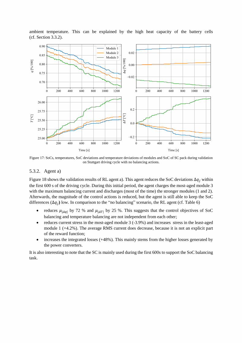
ambient temperature. This can be explained by the high heat capacity of the battery cells

(cf. Section 3.3.2).

Figure 17: SoCs, temperatures, SoC deviations and temperature deviations of modules and SoC of SC pack during validation

on Stuttgart driving cycle with no balancing actions.

5.3.2. Agent a)

Figure 18 shows the validation results of RL agent a). This agent reduces the SoC deviations Δ𝑞𝑗 within

the first 600 s of the driving cycle. During this initial period, the agent charges the most-aged module 3

with the maximum balancing current and discharges (most of the time) the stronger modules (1 and 2).

Afterwards, the magnitude of the control actions is reduced, but the agent is still able to keep the SoC

differences (Δ𝑞𝑗) low. In comparison to the “no balancing” scenario, the RL agent (cf. Table 6)

• reduces 𝜇|𝛥𝑞| by 72 % and 𝜇|𝛥𝑇| by 25 %. This suggests that the control objectives of SoC

balancing and temperature balancing are not independent from each other;

• reduces current stress in the most-aged module 3 (-3.9%) and increases stress in the least-aged

module 1 (+4.2%). The average RMS current does decrease, because it is not an explicit part

of the reward function;

• increases the integrated losses (+48%). This mainly stems from the higher losses generated by

the power converters.

It is also interesting to note that the SC is mainly used during the first 600s to support the SoC balancing

task.

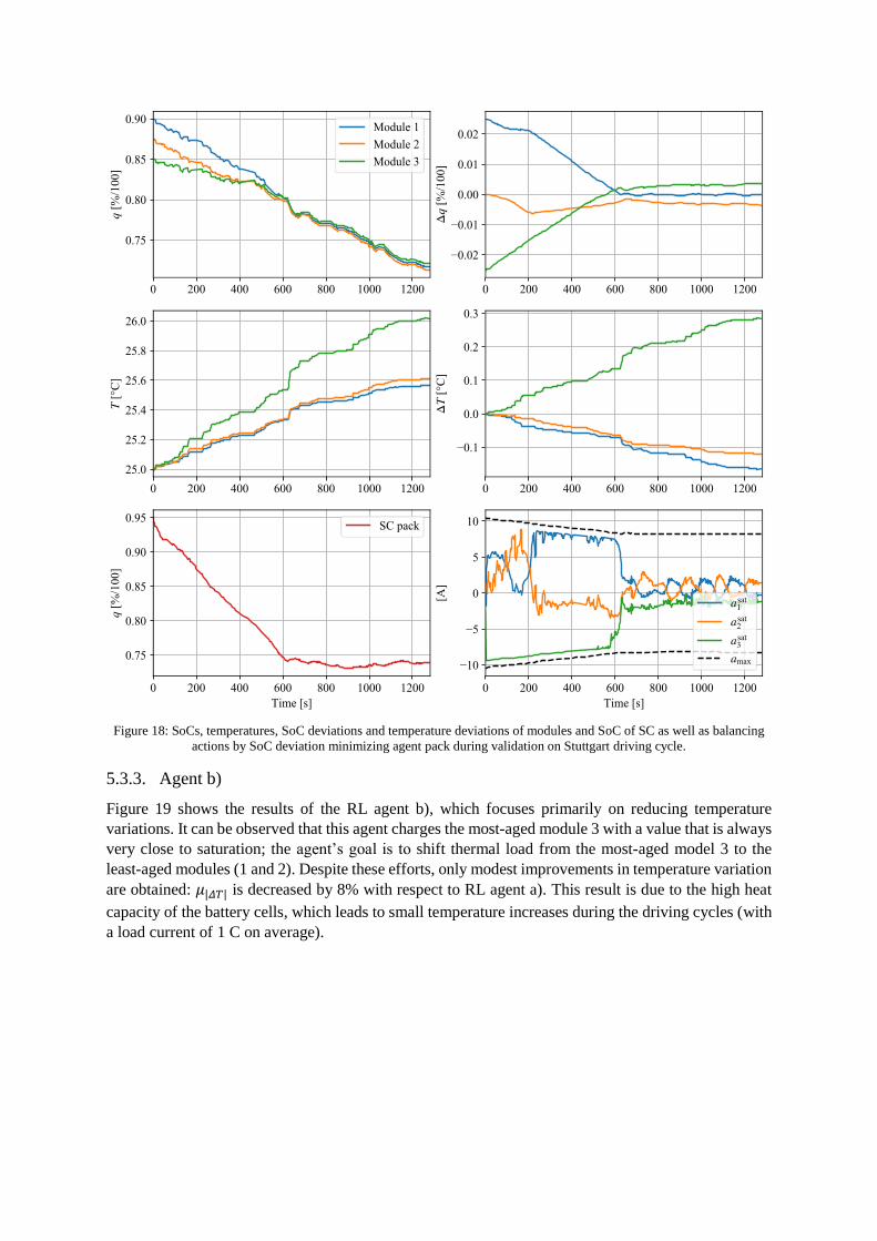
Figure 18: SoCs, temperatures, SoC deviations and temperature deviations of modules and SoC of SC as well as balancing

actions by SoC deviation minimizing agent pack during validation on Stuttgart driving cycle.

5.3.3. Agent b)

Figure 19 shows the results of the RL agent b), which focuses primarily on reducing temperature

variations. It can be observed that this agent charges the most-aged module 3 with a value that is always

very close to saturation; the agent’s goal is to shift thermal load from the most-aged model 3 to the

least-aged modules (1 and 2). Despite these efforts, only modest improvements in temperature variation

are obtained: 𝜇|𝛥𝑇| is decreased by 8% with respect to RL agent a). This result is due to the high heat

capacity of the battery cells, which leads to small temperature increases during the driving cycles (with

a load current of 1 C on average).

Figure 19: SoCs, temperatures, SoC deviations and temperature deviations of modules and SoC of SC as well as balancing

actions by temperature deviation minimizing agent pack during validation on Stuttgart driving cycle.

5.3.4. Agent c)

Figure 20 shows the results of the RL agent c), which focuses on minimization of the current stress.

During the first 200 s, the RL agent extracts energy from the SCs to support the battery cells.

Interestingly, this support is aging-aware: the agent generates actions that decrease the current in the

most-aged modules (2 and 3) and increase the current in the least-aged module (1). After 200 s, the SCs

provide minimum support to the battery pack.

The RL agent c) features the lowest average RMS of all agents, 41.19 A, which represents a reduction

of 1.0 % when compared to the no balancing scenario. At cell level, the RL agent c) reduces the current

of the most-aged module (3) in 4.7 %, while increasing the current in the least-aged module in 2.9 %.

In contrast with the previous test cases, RL agent c) presents more chattering in the control action, which

is due to the reduction of the weight (1/𝑤Δ𝑎). It had therefore less incentive to learn a smooth action

behavior.

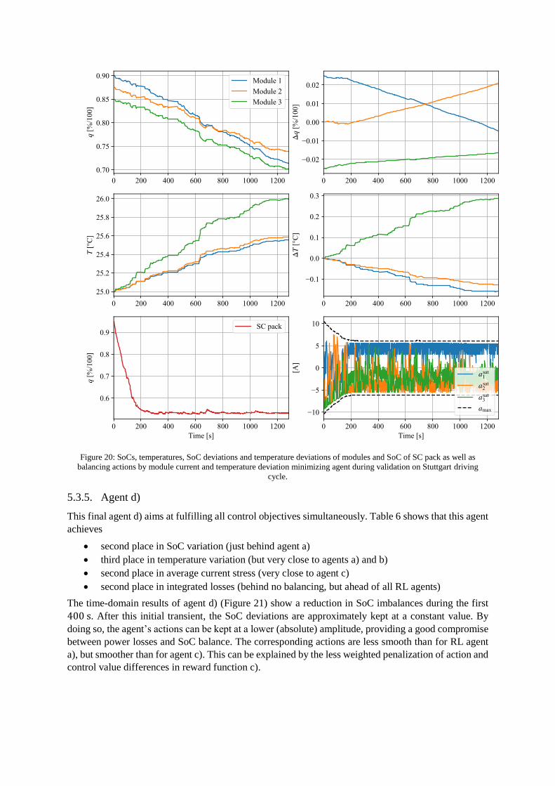
Figure 20: SoCs, temperatures, SoC deviations and temperature deviations of modules and SoC of SC pack as well as

balancing actions by module current and temperature deviation minimizing agent during validation on Stuttgart driving

cycle.

5.3.5. Agent d)

This final agent d) aims at fulfilling all control objectives simultaneously. Table 6 shows that this agent

achieves

• second place in SoC variation (just behind agent a)

• third place in temperature variation (but very close to agents a) and b)

• second place in average current stress (very close to agent c)

• second place in integrated losses (behind no balancing, but ahead of all RL agents)

The time-domain results of agent d) (Figure 21) show a reduction in SoC imbalances during the first

400 s. After this initial transient, the SoC deviations are approximately kept at a constant value. By

doing so, the agent’s actions can be kept at a lower (absolute) amplitude, providing a good compromise

between power losses and SoC balance. The corresponding actions are less smooth than for RL agent

a), but smoother than for agent c). This can be explained by the less weighted penalization of action and

control value differences in reward function c).

Figure 21: SoCs, temperatures, SoC deviations and temperature deviations of modules and SoC of SC pack as well as

balancing actions by module current, temperature deviation, SoC deviation and losses minimizing agent during validation on

Stuttgart driving cycle.

6. Conclusion and Outlook

This work investigated the use of RL to control HBMS. First, a multi-physical model of the HBMS’

components—including power converters, battery and supercapacitors—was implemented in

Modelica. To improve numerical efficiency, a quasi-static model of the power converter was developed.

This allowed us to improve by more than 3000-fold the real-time simulation factor of the HBMS model

and accelerate the RL training. Additionally, the battery model was optimized and validated with

experimental data from NMC cells.

The model was incorporated into a RL toolchain featuring the SAC algorithm. Multiple control

objectives were assessed, yielding RL agents that focus on: a) SoC equalization, b) temperature

equalization, c) age-weighted module current reduction, and d) trade-off between these three objectives

and power losses. To increase the robustness of the obtained RL agents, several randomizations were

incorporated in the training process.

The trained agents were then validated with an unknown driving cycle. In comparison to the scenario

without control, RL agents that prioritize a single objective (a,b,c) were able to reduce SoC deviations

by 72%, temperature deviation by 31%, and the RMS current in the most-aged cell by 4.7%. When all

objectives are traded off simultaneously, the RL agent d) still performed well, reducing the SoC

deviations by 59 %, temperature deviations by 22 % and the RMS current in the most-aged cell by

4.4%. All RL agents increased energy losses due to balancing actions, which is a drawback of the

HBMS.

Additionally, the maximum temperatures in the battery cells were only marginally reduced by the RL

agents due to the large heat capacity of the battery cells. Future work should consider cells with smaller

heat capacity to better assess the potential of RL for thermal management. We also plan to compare the

RL agents’ performance with model-based controllers, incorporate preview information in the RL’s

state vector and perform experimental validation.

Author Contributions: Conceptualization, R.C., J.M., J.B., R.A.; methodology, R.C., J.M., J.B., R.A.;

RL and FMI framework, J.U., J.M.; Modelica models, J.B, J.M.; validation, J.M., R.C.; resources, J.B.,

J.U., R.C.; writing – original draft preparation, J.M., J.B., R.C., J.U., R.A.; writing – review and editing,

J.M., J.B., R.C., J.U., R.A.; visualization, J.M., J.B., R.C., J.U.; supervision, R.C. All authors have read

and agreed to the published version of the manuscript.

Funding: This work was funded by the DLR internal project NGC-A&E.

Acknowledgments: The authors’ thanks go to Tobias Posielek for his feedback and help in scientific

writing.

7. References

[1] International Energy Agency (IEA), "Global EV Outlook 2020," Paris, France, 2020. [Online].

Available: https://www.iea.org/reports/global-ev-outlook-2020.

[2] J. Barreras, D. Frost and D. Howey, "Smart Balancing Systems: An Ultimate Solution to the

Weakest Cell Problem?," in IEEE Vehicular Technology Society Newsletter, 2018.

[3] J. Barreras, C. Pinto, R. de Castro, E. Schaltz, S. Andreasen and R. Araujo, "Multi-Objective

Control of Balancing Systems for Li-Ion Battery Packs: A Paradigm Shift?," in IEEE Vehicle

Power and Propulsion Conference, Coimbra, Portugal, 2014.

[4] E. Chemali, M. Preindl, P. Malysz and A. Emadi, "Electrochemical and Electrostatic Energy

Storage and Management Systems for Electric Drive Vehicles: State-of-the-Art Review and

Future Trends.," IEEE Journal of Emerging and Selected Topics in Power Electronics, vol. 4, no.

3, pp. 1117-1134, 2016.

[5] R. Araujo, R. de Castro, C. Pinto, P. Melo and D. Freitas, "Combined Sizing and Energy

Management in EVs With Batteries and Supercapacitors," IEEE Transactions on Vehicular

Technology, vol. 63, no. 7, pp. 3062-3076, 2014.

[6] Q. Zhang, W. Deng and G. Li, "Stochastic Control of Predictive Power Management for

Battery/Supercapacitor Hybrid Energy Storage Systems of Electric Vehicles," IEEE Transactions

on Industrial Informatics, vol. 14, no. 7, pp. 3023-3030, 2018.

[7] R. de Castro, C. Pinto, J. Barreras, R. Araújo and D. Howey, "Smart and Hybrid Balancing

System: Design, Modeling, and Experimental Demonstration," IEEE Transactions on Vehicular

Technology, vol. 68, no. 12, pp. 11449-11461, 2019.

[8] F. Altaf, B. Egardt and L. Johannesson Mardh, "Load Management of Modular Battery Using

Model Predictive Control: Thermal and State-of-Charge Balancing," IEEE Transactions on

Control Systems Technology, vol. 25, no. 1, pp. 47-62, 2017.

[9] G. L. Plett, Battery Management Systems, Vol. 2: Equivalent-Circuit Methods, Norwood, USA:

Artech House, 2016.

[10] R. de Castro, J. Brembeck and R. E. Araujo, "Nonlinear Control of Dual Half Bridge Converters

in Hybrid Energy Storage Systems," in IEEE Vehicular Power and Propulsion Conference, Gijon,

Spain, 2020.

[11] Y. Li, "Reinforcement Learning Applications," 2019. [Online]. Available:

https://arxiv.org/abs/1908.06973.

[12] D. Liu, "Application of Deep Reinforcement Learning for Battery Design," Master's Thesis,

University of Missouri, USA, 2020.

[13] H. Sun, Z. Fu, F. Tao, L. Zhu and P. Si, "Data-Driven Reinforcement-Learning-Based

Hierarchical Energy Management Strategy for Fuel Cell/Battery/Ultracapacitor Hybrid Electric

Vehicles," Journal of Power Sources, vol. 455, 2020.

[14] B. Xu, J. Shi, S. Li, H. Li and Z. Wang, "Energy Consumption and Battery Aging Minimization

Using a Q-learning Strategy for a Battery/Ultracapacitor Electric Vehicle," 2020. [Online].

Available: https://arxiv.org/abs/2010.14115.

[15] J. Cao, D. Harrold, Z. Fan, T. Morstyn, D. Healey and K. Li, "Deep Reinforcement Learning-

Based Energy Storage Arbitrage With Accurate Lithium-Ion Battery Degradation Model," IEEE

Transactions on Smart Grid, vol. 11, no. 5, pp. 4513-4521, 2020.

[16] S. Park, A. Pozzi, M. Whitmeyer, W. T. Joe, D. M. Raimondo and S. Moura, "Reinforcement

Learning-based Fast Charging Control Strategy for Li-ion Batteries," 2020. [Online]. Available:

https://arxiv.org/abs/2002.02060.

[17] T. Haarnoja, A. Zhou, P. Abbeel and S. Levine, "Soft Actor-Critic: Off-Policy Maximum Entropy

Deep Reinforcement Learning with a Stochastic Actor," in International Conference on Machine

Learning, Stockholm, Sweden, 2018.

[18] A. Hill, A. Raffin, M. Ernestus, A. Gleave, R. Traore, P. Dhariwal, C. Hesse, O. Klimov, A.

Nichol, M. Plappert, A. Radford, J. Schulman, S. Sidor and Y. Wu, Stable Baselines,

https://github.com/hill-a/stable-baselines, 2018.

[19] Modelica Association, "Modelica," 2020. [Online]. Available: http://www.modelica.org.

[Accessed 10 2020].

[20] F. Gao, N. Mugwisi and D. Rogers, "Three Degrees of Freedom Operation of a Dual Half Bridge,"

in European Conference on Power Electronics and Applications, Genova, Italy, 2019.

[21] C. F. A. Pinto, "Sizing and Energy Management of a Distributed Hybrid Energy Storage System

for Electric Vehicles," Ph.D. Thesis, University of Porto, Porto, Portugal, 2018.

[22] D. Graovac, M. Pürschel and A. Kiep, "MOSFET Power Losses Calculation Using the Data-Sheet

Parameters," Infineon Technologies AG, Neubiberg, Germany, 2006.

[23] C. Pinto, J. V. Barreras, E. Schaltz and R. E. Araujo, "Evaluation of Advanced Control for Li-ion

Battery Balancing Systems Using Convex Optimization," IEEE Transactions on Sustainable

Energy, vol. 7, pp. 1703-1717, 2016.

[24] J. Brembeck, "Model Based Energy Management and State Estimation for the Robotic Electric

Vehicle ROboMObil," Ph.D. Thesis, Technical University of Munich, Munich, 2018.

[25] O. Tremblay and L.-A. Dessaint, "Experimental Validation of a Battery Dynamic Model for EV

Applications," World Electric Vehicle Journal, vol. 3, pp. 289-298, 2009.

[26] S. N. Motapon, A. Lupien-Bedard, L.-A. Dessaint, H. Fortin-Blanchette and K. Al-Haddad, "A

Generic Electrothermal Li-ion Battery Model for Rapid Evaluation of Cell Temperature Temporal

Evolution," IEEE Transactions on Industrial Electronics, vol. 64, pp. 998-1008, 2017.

[27] J. Brembeck, "A Physical Model-Based Observer Framework for Nonlinear Constrained State

Estimation Applied to Battery State Estimation," Sensors, vol. 19, no. 20, 4402, 2019.

[28] J. Brembeck, L. M. Ho, A. Schaub, C. Satzger, J. Tobolar, J. Bals and G. Hirzinger, "ROMO –

The Robotic Electric Vehicle," in IAVSD International Symposium on Dynamics of Vehicle on

Roads and Tracks, Manchester, UK, 2011.

[29] A. Pfeiffer, "Optimization Library for Interactive Multi-Criteria Optimization Tasks," in

International MODELICA Conference, Munich, Germany, 2012.

[30] R. Faranda, M. Gallina and D. T. Son, "A New Simplified Model of Double-Layer Capacitors,"

in International Conference on Clean Electrical Power, Capri, Italy, 2007.

[31] J. Tobolar, M. Otter and T. Bünte, "Modelling of Vehicle Powertrains with the Modelica

PowerTrain Library," in Systemanalyse in der Kfz-Antriebstechnik, Augsburg, Germany, 2007.

[32] R. S. Sutton and A. G. Barto, Reinforcement Learning: An Introduction, Second edition ed.,

Cambridge, USA: The MIT Press, 2018.

[33] B. D. Ziebart, "Modeling Purposeful Adaptive Behavior with the Principle of Maximum Causal

Entropy," Ph.D. Thesis, Carnegie Mellon University, Pittsburgh, USA, 2010.

[34] T. Haarnoja, A. Zhou, K. Hartikainen, G. Tucker, S. Ha, J. Tan, V. Kumar, H. Zhu, A. Gupta, P.

Abbeel and S. Levine, "Soft Actor-Critic Algorithms and Applications," 2018. [Online].

Available: https://arxiv.org/abs/1812.05905.

[35] H. v. Hasselt, "Double Q-learning," in International Conference on Neural Information

Processing Systems, Vancouver, Canada, 2010.

[36] S. Fujimoto, H. van Hoof and D. Meger, "Addressing Function Approximation Error in Actor-

Critic Methods," in International Conference on Machine Learning, Stockholm, Sweden, 2018.

[37] S. F. Schuster, M. J. Brand, P. Berg, M. Gleissenberger and A. Jossen, "Lithium-ion Cell-to-Cell

Variation During Battery Electric Vehicle Operation," Journal of Power Sources, vol. 297, pp.

242-251, 2015.

[38] W. Waag, S. Käbitz and D. U. Sauer, "Experimental Investigation of the Lithium-ion Battery

Impedance Characteristic at Various Conditions and Aging States and Its Influence on the

Application," Applied Energy, vol. 102, pp. 885-897, 2013.

[39] X. Glorot, A. Bordes and Y. Bengio, "Deep Sparse Rectifier Neural Networks," in International

Conference on Artificial Intelligence and Statistics, Fort Lauderdale, USA, 2011.