Embed Size (px)
Citation preview
Learning Apache Spark with PythonRelease v1.0
Wenqiang Feng
December 18, 2018

CONTENTS
1 Preface 31.1 About . . . . . . . . . . . . . . . . . . . . . . . . . . . . . . . . . . . . . . . . . . . . . . 31.2 Motivation for this tutorial . . . . . . . . . . . . . . . . . . . . . . . . . . . . . . . . . . . 41.3 Acknowledgement . . . . . . . . . . . . . . . . . . . . . . . . . . . . . . . . . . . . . . . 41.4 Feedback and suggestions . . . . . . . . . . . . . . . . . . . . . . . . . . . . . . . . . . . 4
2 Why Spark with Python ? 52.1 Why Spark? . . . . . . . . . . . . . . . . . . . . . . . . . . . . . . . . . . . . . . . . . . 52.2 Why Spark with Python (PySpark)? . . . . . . . . . . . . . . . . . . . . . . . . . . . . . . 7
3 Configure Running Platform 93.1 Run on Databricks Community Cloud . . . . . . . . . . . . . . . . . . . . . . . . . . . . . 93.2 Configure Spark on Mac and Ubuntu . . . . . . . . . . . . . . . . . . . . . . . . . . . . . 143.3 Configure Spark on Windows . . . . . . . . . . . . . . . . . . . . . . . . . . . . . . . . . 173.4 PySpark With Text Editor or IDE . . . . . . . . . . . . . . . . . . . . . . . . . . . . . . . 173.5 Set up Spark on Cloud . . . . . . . . . . . . . . . . . . . . . . . . . . . . . . . . . . . . . 193.6 Demo Code in this Section . . . . . . . . . . . . . . . . . . . . . . . . . . . . . . . . . . . 21
4 An Introduction to Apache Spark 234.1 Core Concepts . . . . . . . . . . . . . . . . . . . . . . . . . . . . . . . . . . . . . . . . . 234.2 Spark Components . . . . . . . . . . . . . . . . . . . . . . . . . . . . . . . . . . . . . . . 234.3 Architecture . . . . . . . . . . . . . . . . . . . . . . . . . . . . . . . . . . . . . . . . . . 264.4 How Spark Works? . . . . . . . . . . . . . . . . . . . . . . . . . . . . . . . . . . . . . . . 26
5 Programming with RDDs 275.1 Create RDD . . . . . . . . . . . . . . . . . . . . . . . . . . . . . . . . . . . . . . . . . . 275.2 Spark Operations . . . . . . . . . . . . . . . . . . . . . . . . . . . . . . . . . . . . . . . . 31
6 Statistics Preliminary 336.1 Notations . . . . . . . . . . . . . . . . . . . . . . . . . . . . . . . . . . . . . . . . . . . . 336.2 Measurement Formula . . . . . . . . . . . . . . . . . . . . . . . . . . . . . . . . . . . . . 336.3 Statistical Tests . . . . . . . . . . . . . . . . . . . . . . . . . . . . . . . . . . . . . . . . . 34
7 Data Exploration 357.1 Univariate Analysis . . . . . . . . . . . . . . . . . . . . . . . . . . . . . . . . . . . . . . 357.2 Multivariate Analysis . . . . . . . . . . . . . . . . . . . . . . . . . . . . . . . . . . . . . . 49
i
8 Regression 538.1 Linear Regression . . . . . . . . . . . . . . . . . . . . . . . . . . . . . . . . . . . . . . . 538.2 Generalized linear regression . . . . . . . . . . . . . . . . . . . . . . . . . . . . . . . . . 608.3 Decision tree Regression . . . . . . . . . . . . . . . . . . . . . . . . . . . . . . . . . . . . 658.4 Random Forest Regression . . . . . . . . . . . . . . . . . . . . . . . . . . . . . . . . . . . 708.5 Gradient-boosted tree regression . . . . . . . . . . . . . . . . . . . . . . . . . . . . . . . . 70
9 Regularization 719.1 Ridge regression . . . . . . . . . . . . . . . . . . . . . . . . . . . . . . . . . . . . . . . . 719.2 Least Absolute Shrinkage and Selection Operator (LASSO) . . . . . . . . . . . . . . . . . 719.3 Elastic net . . . . . . . . . . . . . . . . . . . . . . . . . . . . . . . . . . . . . . . . . . . 71
10 Classification 7310.1 Logistic regression . . . . . . . . . . . . . . . . . . . . . . . . . . . . . . . . . . . . . . . 7310.2 Decision tree Classification . . . . . . . . . . . . . . . . . . . . . . . . . . . . . . . . . . 8010.3 Random forest Classification . . . . . . . . . . . . . . . . . . . . . . . . . . . . . . . . . . 8710.4 Gradient-boosted tree Classification . . . . . . . . . . . . . . . . . . . . . . . . . . . . . . 9410.5 Naive Bayes Classification . . . . . . . . . . . . . . . . . . . . . . . . . . . . . . . . . . . 95
11 Clustering 9711.1 K-Means Model . . . . . . . . . . . . . . . . . . . . . . . . . . . . . . . . . . . . . . . . 97
12 RFM Analysis 10312.1 RFM Analysis Methodology . . . . . . . . . . . . . . . . . . . . . . . . . . . . . . . . . . 10312.2 Demo . . . . . . . . . . . . . . . . . . . . . . . . . . . . . . . . . . . . . . . . . . . . . . 10412.3 Extension . . . . . . . . . . . . . . . . . . . . . . . . . . . . . . . . . . . . . . . . . . . . 110
13 Text Mining 11713.1 Text Collection . . . . . . . . . . . . . . . . . . . . . . . . . . . . . . . . . . . . . . . . . 11713.2 Text Preprocessing . . . . . . . . . . . . . . . . . . . . . . . . . . . . . . . . . . . . . . . 12413.3 Text Classification . . . . . . . . . . . . . . . . . . . . . . . . . . . . . . . . . . . . . . . 12613.4 Sentiment analysis . . . . . . . . . . . . . . . . . . . . . . . . . . . . . . . . . . . . . . . 13213.5 N-grams and Correlations . . . . . . . . . . . . . . . . . . . . . . . . . . . . . . . . . . . 13813.6 Topic Model: Latent Dirichlet Allocation . . . . . . . . . . . . . . . . . . . . . . . . . . . 138
14 Social Network Analysis 15114.1 Co-occurrence Network . . . . . . . . . . . . . . . . . . . . . . . . . . . . . . . . . . . . 15114.2 Correlation Network . . . . . . . . . . . . . . . . . . . . . . . . . . . . . . . . . . . . . . 156
15 ALS: Stock Portfolio Recommendations 15715.1 Recommender systems . . . . . . . . . . . . . . . . . . . . . . . . . . . . . . . . . . . . . 15715.2 Alternating Least Squares . . . . . . . . . . . . . . . . . . . . . . . . . . . . . . . . . . . 15715.3 Demo . . . . . . . . . . . . . . . . . . . . . . . . . . . . . . . . . . . . . . . . . . . . . . 157
16 Monte Carlo Simulation 16516.1 Simulating Casino Win . . . . . . . . . . . . . . . . . . . . . . . . . . . . . . . . . . . . . 16516.2 Simulating a Random Walk . . . . . . . . . . . . . . . . . . . . . . . . . . . . . . . . . . 167
17 Markov Chain Monte Carlo 175
ii
18 Neural Network 17718.1 Feedforward Neural Network . . . . . . . . . . . . . . . . . . . . . . . . . . . . . . . . . 177
19 My PySpark Package 18119.1 Hierarchical Structure . . . . . . . . . . . . . . . . . . . . . . . . . . . . . . . . . . . . . 18119.2 Set Up . . . . . . . . . . . . . . . . . . . . . . . . . . . . . . . . . . . . . . . . . . . . . 18219.3 ReadMe . . . . . . . . . . . . . . . . . . . . . . . . . . . . . . . . . . . . . . . . . . . . . 182
20 Main Reference 185
Bibliography 187
Index 189
iii

iv
Learning Apache Spark with Python, Release v1.0
Welcome to our Learning Apache Spark with Python note! In these note, you will learn a wide array ofconcepts about PySpark in Data Mining, Text Mining, Machine Leanring and Deep Learning. The PDFversion can be downloaded from HERE.
CONTENTS 1

Learning Apache Spark with Python, Release v1.0
2 CONTENTS
CHAPTER
ONE
PREFACE
1.1 About
1.1.1 About this note
This is a shared repository for Learning Apache Spark Notes. The first version was posted on Github in[Feng2017]. This shared repository mainly contains the self-learning and self-teaching notes from Wenqiangduring his IMA Data Science Fellowship.
In this repository, I try to use the detailed demo code and examples to show how to use each main functions.If you find your work wasn’t cited in this note, please feel free to let me know.
Although I am by no means an data mining programming and Big Data expert, I decided that it would beuseful for me to share what I learned about PySpark programming in the form of easy tutorials with detailedexample. I hope those tutorials will be a valuable tool for your studies.
The tutorials assume that the reader has a preliminary knowledge of programing and Linux. And thisdocument is generated automatically by using sphinx.
1.1.2 About the authors
• Wenqiang Feng
– Data Scientist and PhD in Mathematics
– University of Tennessee at Knoxville
– Email: [email protected]
• Biography
Wenqiang Feng is Data Scientist within DST’s Applied Analytics Group. Dr. Feng’s responsibilitiesinclude providing DST clients with access to cutting-edge skills and technologies, including Big Dataanalytic solutions, advanced analytic and data enhancement techniques and modeling.
Dr. Feng has deep analytic expertise in data mining, analytic systems, machine learning algorithms,business intelligence, and applying Big Data tools to strategically solve industry problems in a cross-functional business. Before joining DST, Dr. Feng was an IMA Data Science Fellow at The Institutefor Mathematics and its Applications (IMA) at the University of Minnesota. While there, he helpedstartup companies make marketing decisions based on deep predictive analytics.
3
Learning Apache Spark with Python, Release v1.0
Dr. Feng graduated from University of Tennessee, Knoxville, with Ph.D. in Computational Mathe-matics and Master’s degree in Statistics. He also holds Master’s degree in Computational Mathematicsfrom Missouri University of Science and Technology (MST) and Master’s degree in Applied Mathe-matics from the University of Science and Technology of China (USTC).
• Declaration
The work of Wenqiang Feng was supported by the IMA, while working at IMA. However, any opin-ion, finding, and conclusions or recommendations expressed in this material are those of the authorand do not necessarily reflect the views of the IMA, UTK and DST.
1.2 Motivation for this tutorial
I was motivated by the IMA Data Science Fellowship project to learn PySpark. After that I was impressedand attracted by the PySpark. And I foud that:
1. It is no exaggeration to say that Spark is the most powerful Bigdata tool.
2. However, I still found that learning Spark was a difficult process. I have to Google it and identifywhich one is true. And it was hard to find detailed examples which I can easily learned the fullprocess in one file.
3. Good sources are expensive for a graduate student.
1.3 Acknowledgement
At here, I would like to thank Ming Chen, Jian Sun and Zhongbo Li at the University of Tennessee atKnoxville for the valuable disscussion and thank the generous anonymous authors for providing the detailedsolutions and source code on the internet. Without those help, this repository would not have been possibleto be made. Wenqiang also would like to thank the Institute for Mathematics and Its Applications (IMA) atUniversity of Minnesota, Twin Cities for support during his IMA Data Scientist Fellow visit.
1.4 Feedback and suggestions
Your comments and suggestions are highly appreciated. I am more than happy to receive corrections, sug-gestions or feedbacks through email ([email protected]) for improvements.
4 Chapter 1. Preface
CHAPTER
TWO
WHY SPARK WITH PYTHON ?
Note: Sharpening the knife longer can make it easier to hack the firewood – old Chinese proverb
I want to answer this question from the following two parts:
2.1 Why Spark?
I think the following four main reasons form Apache Spark™ official website are good enough to convinceyou to use Spark.
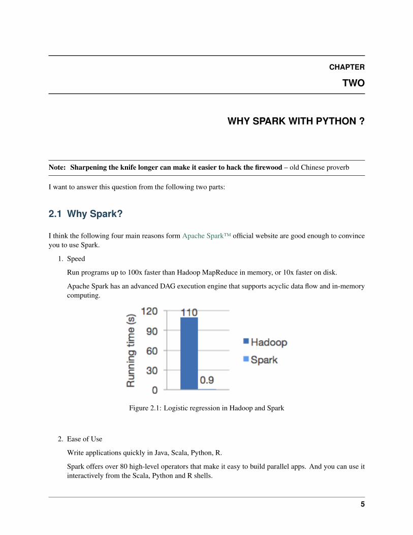
1. Speed
Run programs up to 100x faster than Hadoop MapReduce in memory, or 10x faster on disk.
Apache Spark has an advanced DAG execution engine that supports acyclic data flow and in-memorycomputing.
Figure 2.1: Logistic regression in Hadoop and Spark
2. Ease of Use
Write applications quickly in Java, Scala, Python, R.
Spark offers over 80 high-level operators that make it easy to build parallel apps. And you can use itinteractively from the Scala, Python and R shells.
5
Learning Apache Spark with Python, Release v1.0
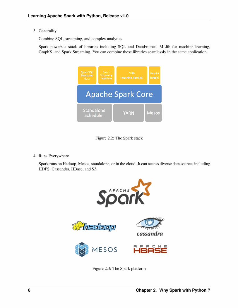
3. Generality
Combine SQL, streaming, and complex analytics.
Spark powers a stack of libraries including SQL and DataFrames, MLlib for machine learning,GraphX, and Spark Streaming. You can combine these libraries seamlessly in the same application.
Figure 2.2: The Spark stack
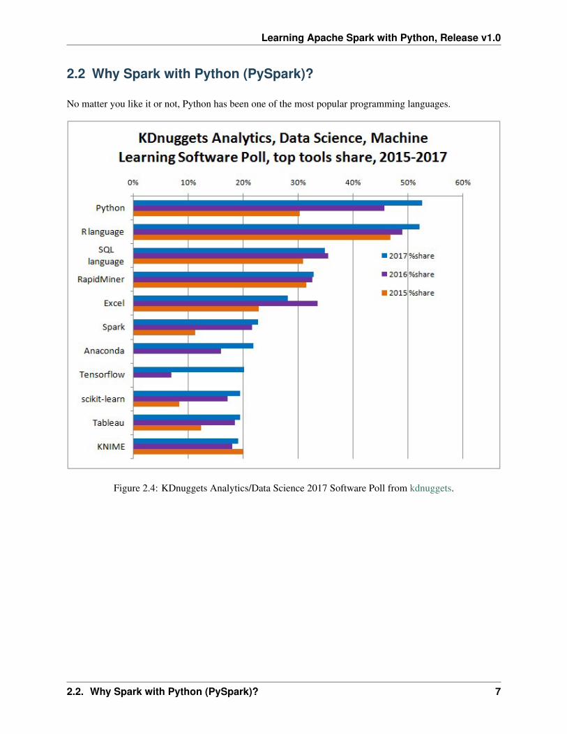
4. Runs Everywhere
Spark runs on Hadoop, Mesos, standalone, or in the cloud. It can access diverse data sources includingHDFS, Cassandra, HBase, and S3.
Figure 2.3: The Spark platform
6 Chapter 2. Why Spark with Python ?
Learning Apache Spark with Python, Release v1.0
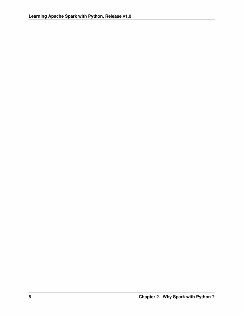
2.2 Why Spark with Python (PySpark)?
No matter you like it or not, Python has been one of the most popular programming languages.
Figure 2.4: KDnuggets Analytics/Data Science 2017 Software Poll from kdnuggets.
2.2. Why Spark with Python (PySpark)? 7
Learning Apache Spark with Python, Release v1.0
8 Chapter 2. Why Spark with Python ?
CHAPTER
THREE
CONFIGURE RUNNING PLATFORM
Note: Good tools are prerequisite to the successful execution of a job. – old Chinese proverb
A good programming platform can save you lots of troubles and time. Herein I will only present how toinstall my favorite programming platform and only show the easiest way which I know to set it up on Linuxsystem. If you want to install on the other operator system, you can Google it. In this section, you may learnhow to set up Pyspark on the corresponding programming platform and package.
3.1 Run on Databricks Community Cloud
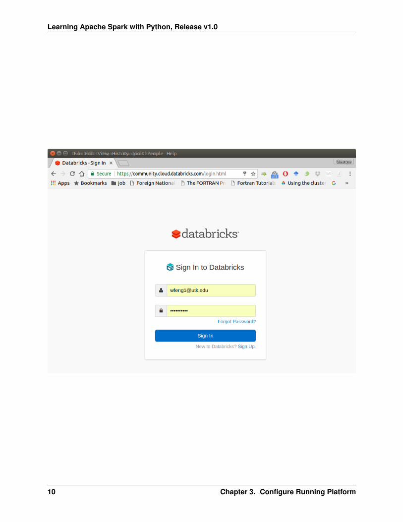
If you don’t have any experience with Linux or Unix operator system, I would love to recommend you touse Spark on Databricks Community Cloud. Since you do not need to setup the Spark and it’s totally freefor Community Edition. Please follow the steps listed below.
1. Sign up a account at: https://community.cloud.databricks.com/login.html
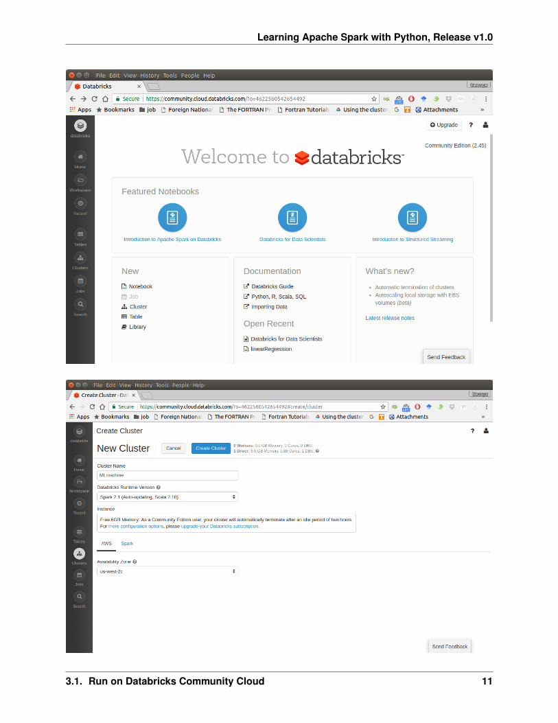
2. Sign in with your account, then you can creat your cluster(machine), table(dataset) andnotebook(code).
3. Create your cluster where your code will run
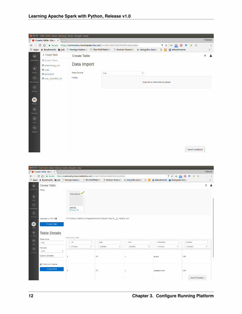
4. Import your dataset
Note: You need to save the path which appears at Uploaded to DBFS: /File-Store/tables/05rmhuqv1489687378010/. Since we will use this path to load the dataset.
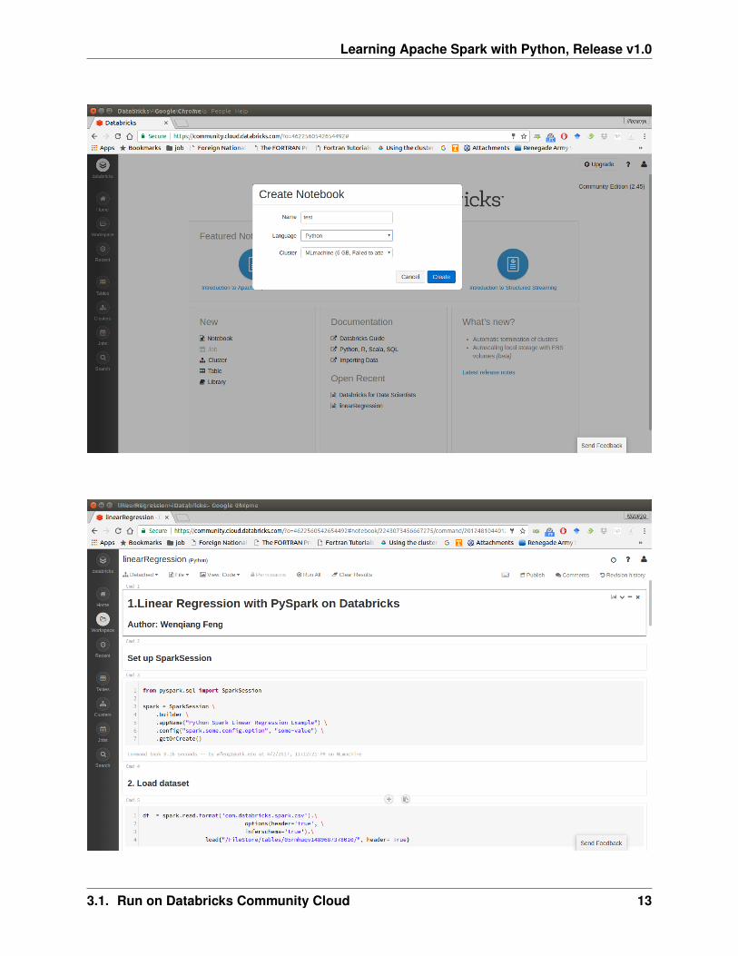
5. Creat your notebook
9
Learning Apache Spark with Python, Release v1.0
10 Chapter 3. Configure Running Platform
Learning Apache Spark with Python, Release v1.0
3.1. Run on Databricks Community Cloud 11
Learning Apache Spark with Python, Release v1.0
12 Chapter 3. Configure Running Platform
Learning Apache Spark with Python, Release v1.0
3.1. Run on Databricks Community Cloud 13
Learning Apache Spark with Python, Release v1.0
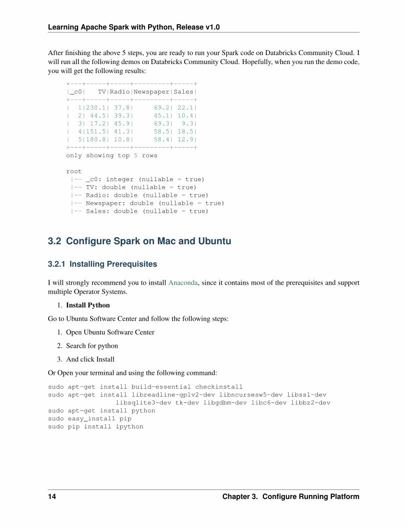
After finishing the above 5 steps, you are ready to run your Spark code on Databricks Community Cloud. Iwill run all the following demos on Databricks Community Cloud. Hopefully, when you run the demo code,you will get the following results:
+---+-----+-----+---------+-----+|_c0| TV|Radio|Newspaper|Sales|+---+-----+-----+---------+-----+| 1|230.1| 37.8| 69.2| 22.1|| 2| 44.5| 39.3| 45.1| 10.4|| 3| 17.2| 45.9| 69.3| 9.3|| 4|151.5| 41.3| 58.5| 18.5|| 5|180.8| 10.8| 58.4| 12.9|+---+-----+-----+---------+-----+only showing top 5 rows
root|-- _c0: integer (nullable = true)|-- TV: double (nullable = true)|-- Radio: double (nullable = true)|-- Newspaper: double (nullable = true)|-- Sales: double (nullable = true)
3.2 Configure Spark on Mac and Ubuntu
3.2.1 Installing Prerequisites
I will strongly recommend you to install Anaconda, since it contains most of the prerequisites and supportmultiple Operator Systems.
1. Install Python
Go to Ubuntu Software Center and follow the following steps:
1. Open Ubuntu Software Center
2. Search for python
3. And click Install
Or Open your terminal and using the following command:
sudo apt-get install build-essential checkinstallsudo apt-get install libreadline-gplv2-dev libncursesw5-dev libssl-dev
libsqlite3-dev tk-dev libgdbm-dev libc6-dev libbz2-devsudo apt-get install pythonsudo easy_install pipsudo pip install ipython
14 Chapter 3. Configure Running Platform
Learning Apache Spark with Python, Release v1.0
3.2.2 Install Java
Java is used by many other softwares. So it is quite possible that you have already installed it. You can byusing the following command in Command Prompt:
java -version
Otherwise, you can follow the steps in How do I install Java for my Mac? to install java on Mac and use thefollowing command in Command Prompt to install on Ubuntu:
sudo apt-add-repository ppa:webupd8team/javasudo apt-get updatesudo apt-get install oracle-java8-installer
3.2.3 Install Java SE Runtime Environment
I installed ORACLE Java JDK.
Warning: Installing Java and Java SE Runtime Environment steps are very important, sinceSpark is a domain-specific language written in Java.
You can check if your Java is available and find it’s version by using the following command in CommandPrompt:
java -version
If your Java is installed successfully, you will get the similar results as follows:
java version "1.8.0_131"Java(TM) SE Runtime Environment (build 1.8.0_131-b11)Java HotSpot(TM) 64-Bit Server VM (build 25.131-b11, mixed mode)
3.2.4 Install Apache Spark
Actually, the Pre-build version doesn’t need installation. You can use it when you unpack it.
1. Download: You can get the Pre-built Apache Spark™ from Download Apache Spark™.
2. Unpack: Unpack the Apache Spark™ to the path where you want to install the Spark.
3. Test: Test the Prerequisites: change the directionspark-#.#.#-bin-hadoop#.#/bin and run
./pyspark
Python 2.7.13 |Anaconda 4.4.0 (x86_64)| (default, Dec 20 2016, 23:05:08)[GCC 4.2.1 Compatible Apple LLVM 6.0 (clang-600.0.57)] on darwinType "help", "copyright", "credits" or "license" for more information.Anaconda is brought to you by Continuum Analytics.Please check out: http://continuum.io/thanks and https://anaconda.orgUsing Spark’s default log4j profile: org/apache/spark/log4j-defaults.properties
3.2. Configure Spark on Mac and Ubuntu 15
Learning Apache Spark with Python, Release v1.0
Setting default log level to "WARN".To adjust logging level use sc.setLogLevel(newLevel). For SparkR,use setLogLevel(newLevel).17/08/30 13:30:12 WARN NativeCodeLoader: Unable to load native-hadooplibrary for your platform... using builtin-java classes where applicable17/08/30 13:30:17 WARN ObjectStore: Failed to get database global_temp,returning NoSuchObjectExceptionWelcome to
____ __/ __/__ ___ _____/ /___\ \/ _ \/ _ ‘/ __/ ’_/
/__ / .__/\_,_/_/ /_/\_\ version 2.1.1/_/
Using Python version 2.7.13 (default, Dec 20 2016 23:05:08)SparkSession available as ’spark’.
3.2.5 Configure the Spark
1. Mac Operator System: open your bash_profile in Terminal
vim ~/.bash_profile
And add the following lines to your bash_profile (remember to change the path)
# add for sparkexport SPARK_HOME=your_spark_installation_pathexport PATH=$PATH:$SPARK_HOME/bin:$SPARK_HOME/sbinexport PATH=$PATH:$SPARK_HOME/binexport PYSPARK_DRIVE_PYTHON="jupyter"export PYSPARK_DRIVE_PYTHON_OPTS="notebook"
At last, remember to source your bash_profile
source ~/.bash_profile
2. Ubuntu Operator Sysytem: open your bashrc in Terminal
vim ~/.bashrc
And add the following lines to your bashrc (remember to change the path)
# add for sparkexport SPARK_HOME=your_spark_installation_pathexport PATH=$PATH:$SPARK_HOME/bin:$SPARK_HOME/sbinexport PATH=$PATH:$SPARK_HOME/binexport PYSPARK_DRIVE_PYTHON="jupyter"export PYSPARK_DRIVE_PYTHON_OPTS="notebook"
At last, remember to source your bashrc
source ~/.bashrc
16 Chapter 3. Configure Running Platform
Learning Apache Spark with Python, Release v1.0
3.3 Configure Spark on Windows
Installing open source software on Windows is always a nightmare for me. Thanks for Deelesh Mandloi.You can follow the detailed procedures in the blog Getting Started with PySpark on Windows to install theApache Spark™ on your Windows Operator System.
3.4 PySpark With Text Editor or IDE
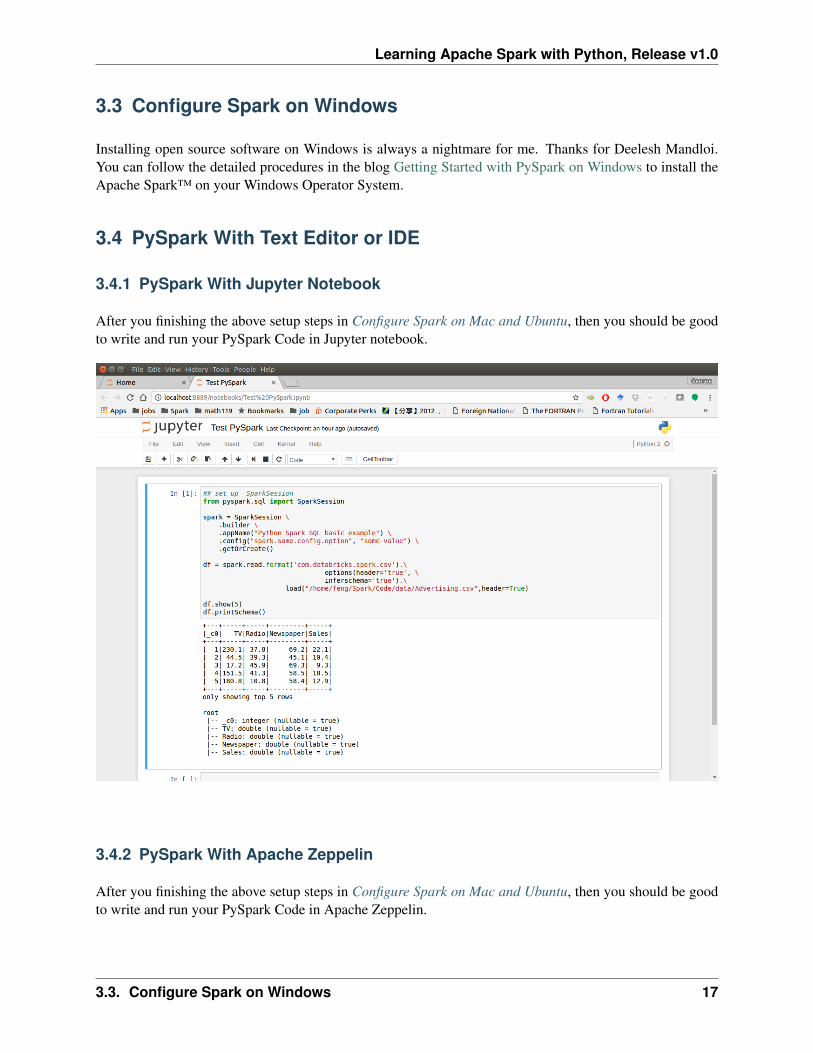
3.4.1 PySpark With Jupyter Notebook
After you finishing the above setup steps in Configure Spark on Mac and Ubuntu, then you should be goodto write and run your PySpark Code in Jupyter notebook.
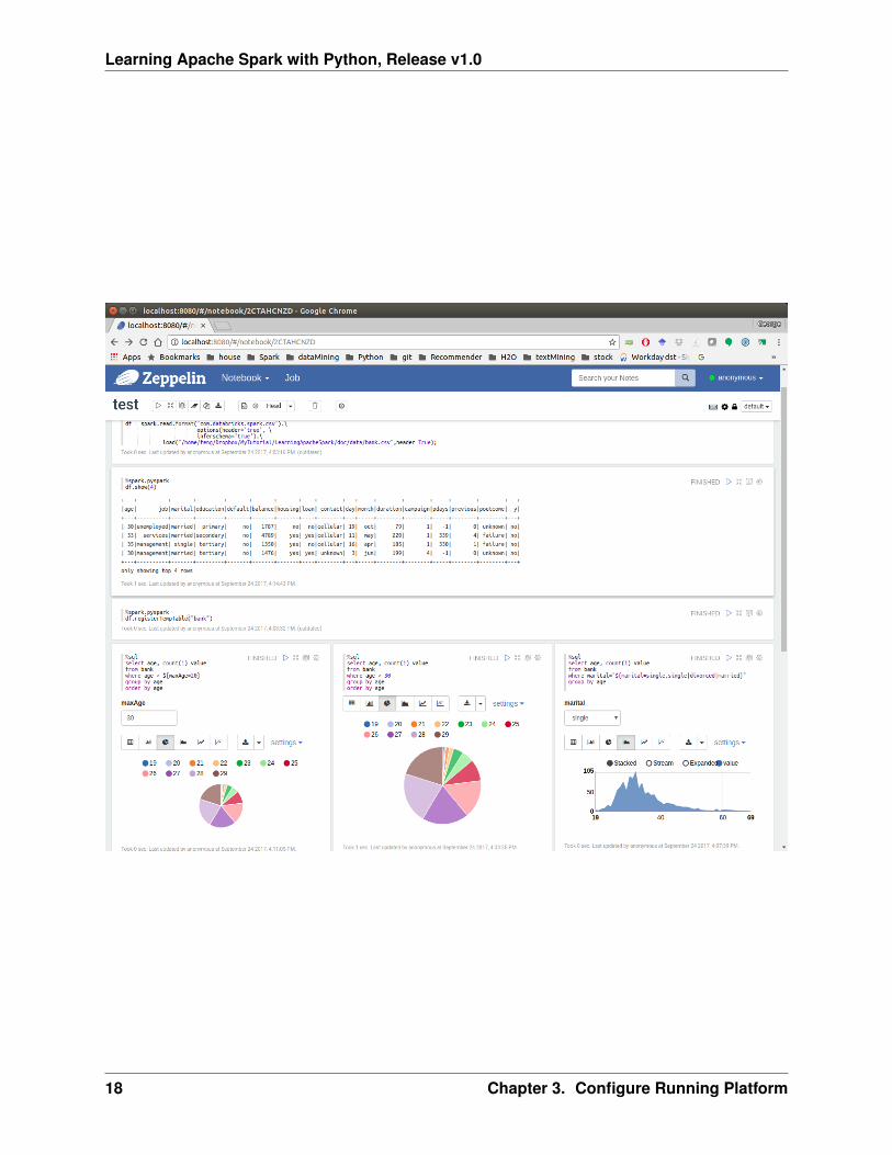
3.4.2 PySpark With Apache Zeppelin
After you finishing the above setup steps in Configure Spark on Mac and Ubuntu, then you should be goodto write and run your PySpark Code in Apache Zeppelin.
3.3. Configure Spark on Windows 17
Learning Apache Spark with Python, Release v1.0
18 Chapter 3. Configure Running Platform

Learning Apache Spark with Python, Release v1.0
3.4.3 PySpark With Sublime Text
After you finishing the above setup steps in Configure Spark on Mac and Ubuntu, then you should be goodto use Sublime Text to write your PySpark Code and run your code as a normal python code in Terminal.
python test_pyspark.py
Then you should get the output results in your terminal.
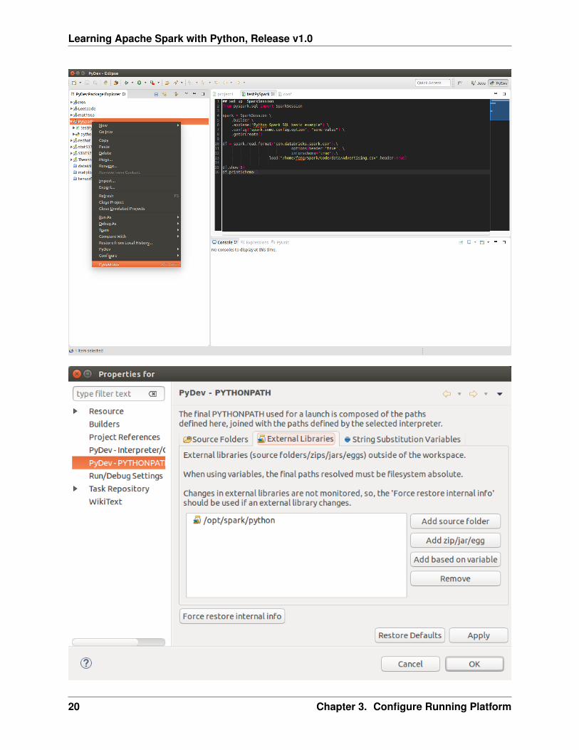
3.4.4 PySpark With Eclipse
If you want to run PySpark code on Eclipse, you need to add the paths for the External Libraries for yourCurrent Project as follows:
1. Open the properties of your project
2. Add the paths for the External Libraries
And then you should be good to run your code on Eclipse with PyDev.
3.5 Set up Spark on Cloud
Following the setup steps in Configure Spark on Mac and Ubuntu, you can set up your own cluster on thecloud, for example AWS, Google Cloud. Actually, for those clouds, they have their own Big Data tool. Yoncan run them directly whitout any setting just like Databricks Community Cloud. If you want more details,please feel free to contact with me.
3.5. Set up Spark on Cloud 19
Learning Apache Spark with Python, Release v1.0
20 Chapter 3. Configure Running Platform
Learning Apache Spark with Python, Release v1.0
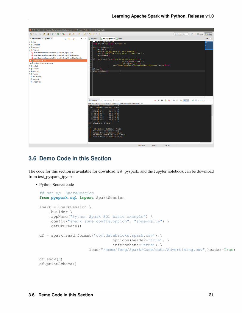
3.6 Demo Code in this Section
The code for this section is available for download test_pyspark, and the Jupyter notebook can be downloadfrom test_pyspark_ipynb.
• Python Source code
## set up SparkSessionfrom pyspark.sql import SparkSession
spark = SparkSession \.builder \.appName("Python Spark SQL basic example") \.config("spark.some.config.option", "some-value") \.getOrCreate()
df = spark.read.format(’com.databricks.spark.csv’).\options(header=’true’, \inferschema=’true’).\
load("/home/feng/Spark/Code/data/Advertising.csv",header=True)
df.show(5)df.printSchema()
3.6. Demo Code in this Section 21
Learning Apache Spark with Python, Release v1.0
22 Chapter 3. Configure Running Platform
CHAPTER
FOUR
AN INTRODUCTION TO APACHE SPARK
Note: Know yourself and know your enemy, and you will never be defeated – idiom, from Sunzi’s Artof War
4.1 Core Concepts
Most of the following content comes from [Kirillov2016]. So the copyright belongs to Anton Kirillov. Iwill refer you to get more details from Apache Spark core concepts, architecture and internals.
Before diving deep into how Apache Spark works, lets understand the jargon of Apache Spark
• Job: A piece of code which reads some input from HDFS or local, performs some computation on thedata and writes some output data.
• Stages: Jobs are divided into stages. Stages are classified as a Map or reduce stages (Its easier tounderstand if you have worked on Hadoop and want to correlate). Stages are divided based on com-putational boundaries, all computations (operators) cannot be Updated in a single Stage. It happensover many stages.
• Tasks: Each stage has some tasks, one task per partition. One task is executed on one partition of dataon one executor (machine).
• DAG: DAG stands for Directed Acyclic Graph, in the present context its a DAG of operators.
• Executor: The process responsible for executing a task.
• Master: The machine on which the Driver program runs
• Slave: The machine on which the Executor program runs
4.2 Spark Components
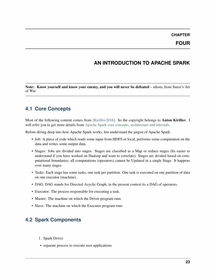
1. Spark Driver
• separate process to execute user applications
23
Learning Apache Spark with Python, Release v1.0
24 Chapter 4. An Introduction to Apache Spark
Learning Apache Spark with Python, Release v1.0
• creates SparkContext to schedule jobs execution and negotiate with cluster manager
2. Executors
• run tasks scheduled by driver
• store computation results in memory, on disk or off-heap
• interact with storage systems
3. Cluster Manager
• Mesos
• YARN
• Spark Standalone
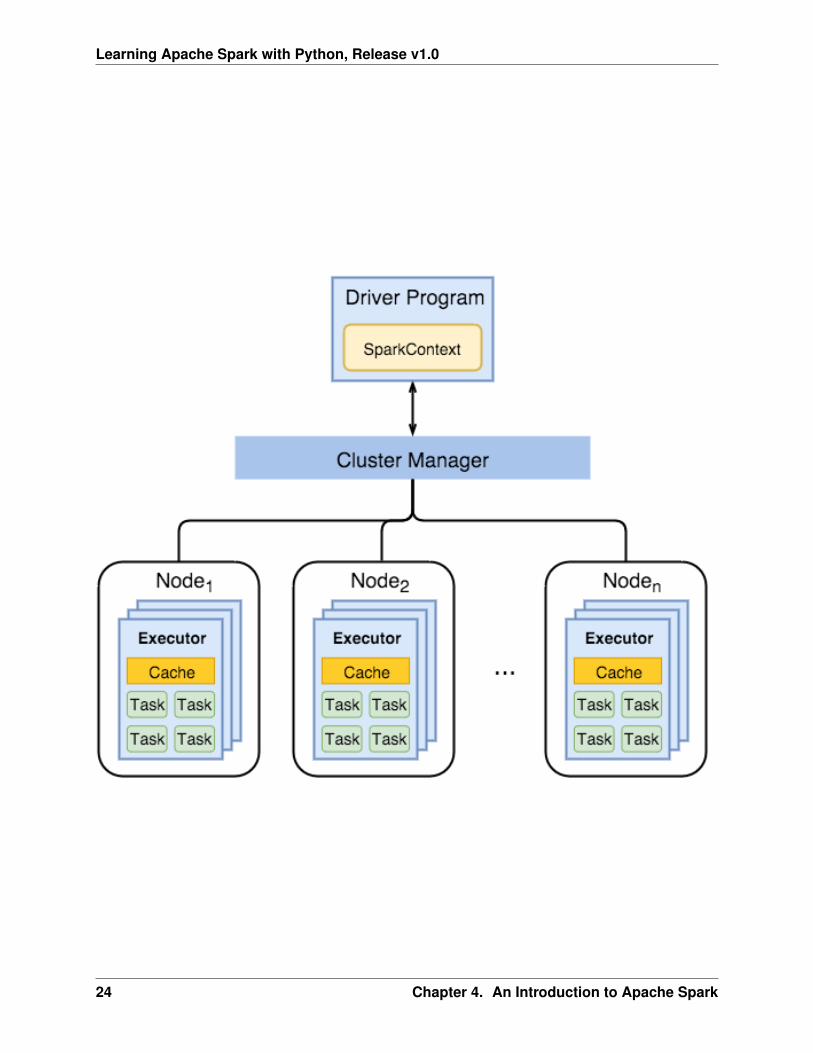
Spark Driver contains more components responsible for translation of user code into actual jobs executedon cluster:
• SparkContext
– represents the connection to a Spark cluster, and can be used to create RDDs, accu-mulators and broadcast variables on that cluster
• DAGScheduler
– computes a DAG of stages for each job and submits them to TaskScheduler deter-mines preferred locations for tasks (based on cache status or shuffle files locations)and finds minimum schedule to run the jobs
• TaskScheduler
– responsible for sending tasks to the cluster, running them, retrying if there are failures,and mitigating stragglers
• SchedulerBackend
– backend interface for scheduling systems that allows plugging in different implemen-tations(Mesos, YARN, Standalone, local)
4.2. Spark Components 25
Learning Apache Spark with Python, Release v1.0
• BlockManager
– provides interfaces for putting and retrieving blocks both locally and remotely intovarious stores (memory, disk, and off-heap)
4.3 Architecture
4.4 How Spark Works?
Spark has a small code base and the system is divided in various layers. Each layer has some responsibilities.The layers are independent of each other.
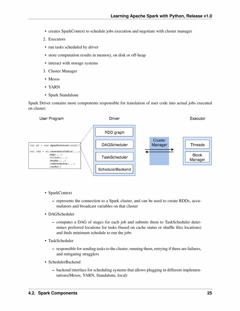
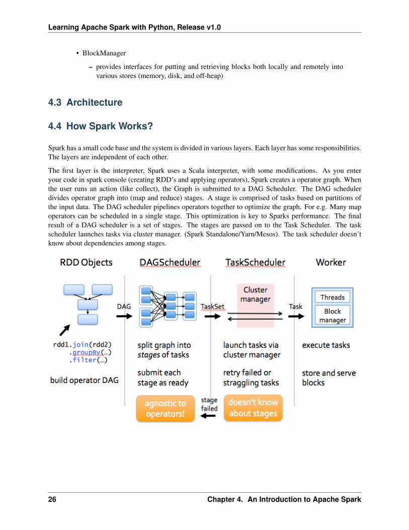
The first layer is the interpreter, Spark uses a Scala interpreter, with some modifications. As you enteryour code in spark console (creating RDD’s and applying operators), Spark creates a operator graph. Whenthe user runs an action (like collect), the Graph is submitted to a DAG Scheduler. The DAG schedulerdivides operator graph into (map and reduce) stages. A stage is comprised of tasks based on partitions ofthe input data. The DAG scheduler pipelines operators together to optimize the graph. For e.g. Many mapoperators can be scheduled in a single stage. This optimization is key to Sparks performance. The finalresult of a DAG scheduler is a set of stages. The stages are passed on to the Task Scheduler. The taskscheduler launches tasks via cluster manager. (Spark Standalone/Yarn/Mesos). The task scheduler doesn’tknow about dependencies among stages.
26 Chapter 4. An Introduction to Apache Spark

CHAPTER
FIVE
PROGRAMMING WITH RDDS
Note: If you only know yourself, but not your opponent, you may win or may lose. If you knowneither yourself nor your enemy, you will always endanger yourself – idiom, from Sunzi’s Art of War
RDD represents Resilient Distributed Dataset. An RDD in Spark is simply an immutable distributedcollection of objects sets. Each RDD is split into multiple partitions (similar pattern with smaller sets),which may be computed on different nodes of the cluster.
5.1 Create RDD
Usually, there are two popular way to create the RDDs: loading an external dataset, or distributing a setof collection of objects. The following examples show some simplest ways to create RDDs by usingparallelize() fucntion which takes an already existing collection in your program and pass the sameto the Spark Context.
1. By using parallelize( ) fucntion
from pyspark.sql import SparkSession
spark = SparkSession \.builder \.appName("Python Spark create RDD example") \.config("spark.some.config.option", "some-value") \.getOrCreate()
df = spark.sparkContext.parallelize([(1, 2, 3, ’a b c’),(4, 5, 6, ’d e f’),(7, 8, 9, ’g h i’)]).toDF([’col1’, ’col2’, ’col3’,’col4’])
Then you will get the RDD data:
df.show()
+----+----+----+-----+|col1|col2|col3| col4|+----+----+----+-----+| 1| 2| 3|a b c|| 4| 5| 6|d e f|
27
Learning Apache Spark with Python, Release v1.0
| 7| 8| 9|g h i|+----+----+----+-----+
from pyspark.sql import SparkSession
spark = SparkSession \.builder \.appName("Python Spark create RDD example") \.config("spark.some.config.option", "some-value") \.getOrCreate()
myData = spark.sparkContext.parallelize([(1,2), (3,4), (5,6), (7,8), (9,10)])
Then you will get the RDD data:
myData.collect()
[(1, 2), (3, 4), (5, 6), (7, 8), (9, 10)]
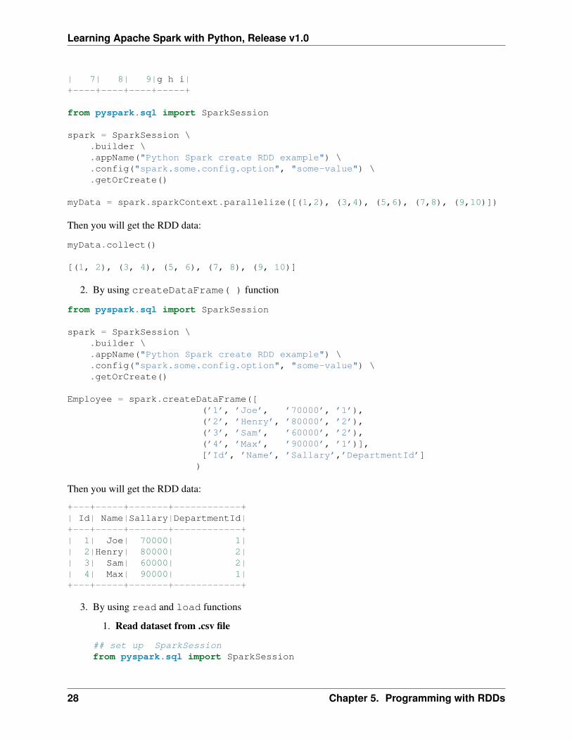
2. By using createDataFrame( ) function
from pyspark.sql import SparkSession
spark = SparkSession \.builder \.appName("Python Spark create RDD example") \.config("spark.some.config.option", "some-value") \.getOrCreate()
Employee = spark.createDataFrame([(’1’, ’Joe’, ’70000’, ’1’),(’2’, ’Henry’, ’80000’, ’2’),(’3’, ’Sam’, ’60000’, ’2’),(’4’, ’Max’, ’90000’, ’1’)],[’Id’, ’Name’, ’Sallary’,’DepartmentId’]
)
Then you will get the RDD data:
+---+-----+-------+------------+| Id| Name|Sallary|DepartmentId|+---+-----+-------+------------+| 1| Joe| 70000| 1|| 2|Henry| 80000| 2|| 3| Sam| 60000| 2|| 4| Max| 90000| 1|+---+-----+-------+------------+
3. By using read and load functions
1. Read dataset from .csv file
## set up SparkSessionfrom pyspark.sql import SparkSession
28 Chapter 5. Programming with RDDs
Learning Apache Spark with Python, Release v1.0
spark = SparkSession \.builder \.appName("Python Spark create RDD example") \.config("spark.some.config.option", "some-value") \.getOrCreate()
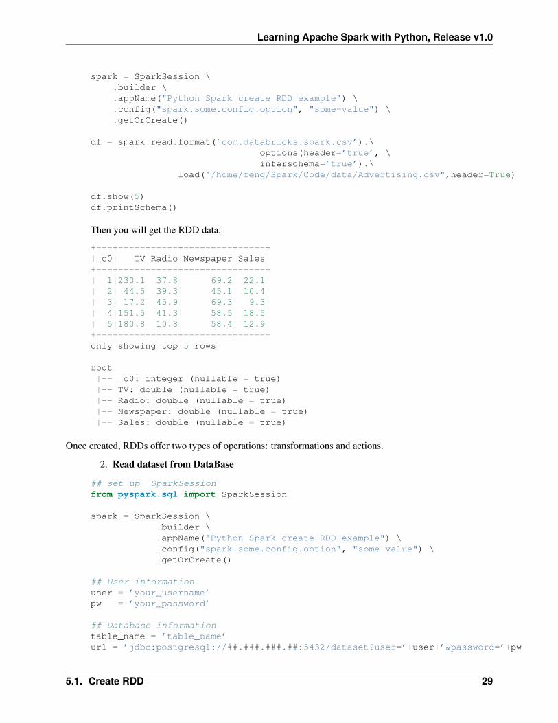
df = spark.read.format(’com.databricks.spark.csv’).\options(header=’true’, \inferschema=’true’).\
load("/home/feng/Spark/Code/data/Advertising.csv",header=True)
df.show(5)df.printSchema()
Then you will get the RDD data:
+---+-----+-----+---------+-----+|_c0| TV|Radio|Newspaper|Sales|+---+-----+-----+---------+-----+| 1|230.1| 37.8| 69.2| 22.1|| 2| 44.5| 39.3| 45.1| 10.4|| 3| 17.2| 45.9| 69.3| 9.3|| 4|151.5| 41.3| 58.5| 18.5|| 5|180.8| 10.8| 58.4| 12.9|+---+-----+-----+---------+-----+only showing top 5 rows
root|-- _c0: integer (nullable = true)|-- TV: double (nullable = true)|-- Radio: double (nullable = true)|-- Newspaper: double (nullable = true)|-- Sales: double (nullable = true)
Once created, RDDs offer two types of operations: transformations and actions.
2. Read dataset from DataBase
## set up SparkSessionfrom pyspark.sql import SparkSession
spark = SparkSession \.builder \.appName("Python Spark create RDD example") \.config("spark.some.config.option", "some-value") \.getOrCreate()
## User informationuser = ’your_username’pw = ’your_password’
## Database informationtable_name = ’table_name’url = ’jdbc:postgresql://##.###.###.##:5432/dataset?user=’+user+’&password=’+pw
5.1. Create RDD 29
Learning Apache Spark with Python, Release v1.0
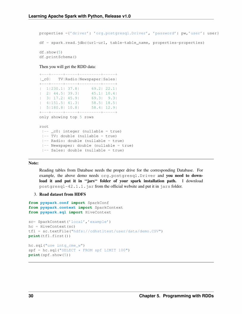
properties ={’driver’: ’org.postgresql.Driver’, ’password’: pw,’user’: user}
df = spark.read.jdbc(url=url, table=table_name, properties=properties)
df.show(5)df.printSchema()
Then you will get the RDD data:
+---+-----+-----+---------+-----+|_c0| TV|Radio|Newspaper|Sales|+---+-----+-----+---------+-----+| 1|230.1| 37.8| 69.2| 22.1|| 2| 44.5| 39.3| 45.1| 10.4|| 3| 17.2| 45.9| 69.3| 9.3|| 4|151.5| 41.3| 58.5| 18.5|| 5|180.8| 10.8| 58.4| 12.9|+---+-----+-----+---------+-----+only showing top 5 rows
root|-- _c0: integer (nullable = true)|-- TV: double (nullable = true)|-- Radio: double (nullable = true)|-- Newspaper: double (nullable = true)|-- Sales: double (nullable = true)
Note:
Reading tables from Database needs the proper drive for the corresponding Database. Forexample, the above demo needs org.postgresql.Driver and you need to down-load it and put it in ‘‘jars‘‘ folder of your spark installation path. I downloadpostgresql-42.1.1.jar from the official website and put it in jars folder.
3. Read dataset from HDFS
from pyspark.conf import SparkConffrom pyspark.context import SparkContextfrom pyspark.sql import HiveContext
sc= SparkContext(’local’,’example’)hc = HiveContext(sc)tf1 = sc.textFile("hdfs://cdhstltest/user/data/demo.CSV")print(tf1.first())
hc.sql("use intg_cme_w")spf = hc.sql("SELECT * FROM spf LIMIT 100")print(spf.show(5))
30 Chapter 5. Programming with RDDs
Learning Apache Spark with Python, Release v1.0
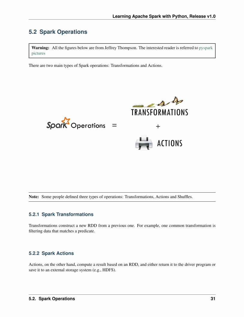
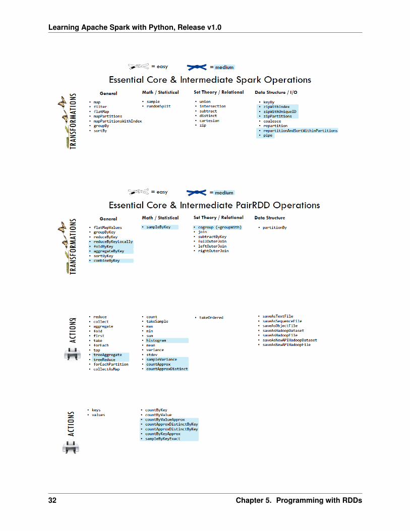
5.2 Spark Operations
Warning: All the figures below are from Jeffrey Thompson. The interested reader is referred to pysparkpictures
There are two main types of Spark operations: Transformations and Actions.
Note: Some people defined three types of operations: Transformations, Actions and Shuffles.
5.2.1 Spark Transformations
Transformations construct a new RDD from a previous one. For example, one common transformation isfiltering data that matches a predicate.
5.2.2 Spark Actions
Actions, on the other hand, compute a result based on an RDD, and either return it to the driver program orsave it to an external storage system (e.g., HDFS).
5.2. Spark Operations 31
Learning Apache Spark with Python, Release v1.0
32 Chapter 5. Programming with RDDs
CHAPTER
SIX
STATISTICS PRELIMINARY
Note: If you only know yourself, but not your opponent, you may win or may lose. If you knowneither yourself nor your enemy, you will always endanger yourself – idiom, from Sunzi’s Art of War
6.1 Notations
• m : the number of the samples
• n : the number of the features
• 𝑦𝑖 : i-th label
• 𝑦 = 1𝑚
∑︀𝑛𝑖=1 𝑦𝑖: the mean of 𝑦.
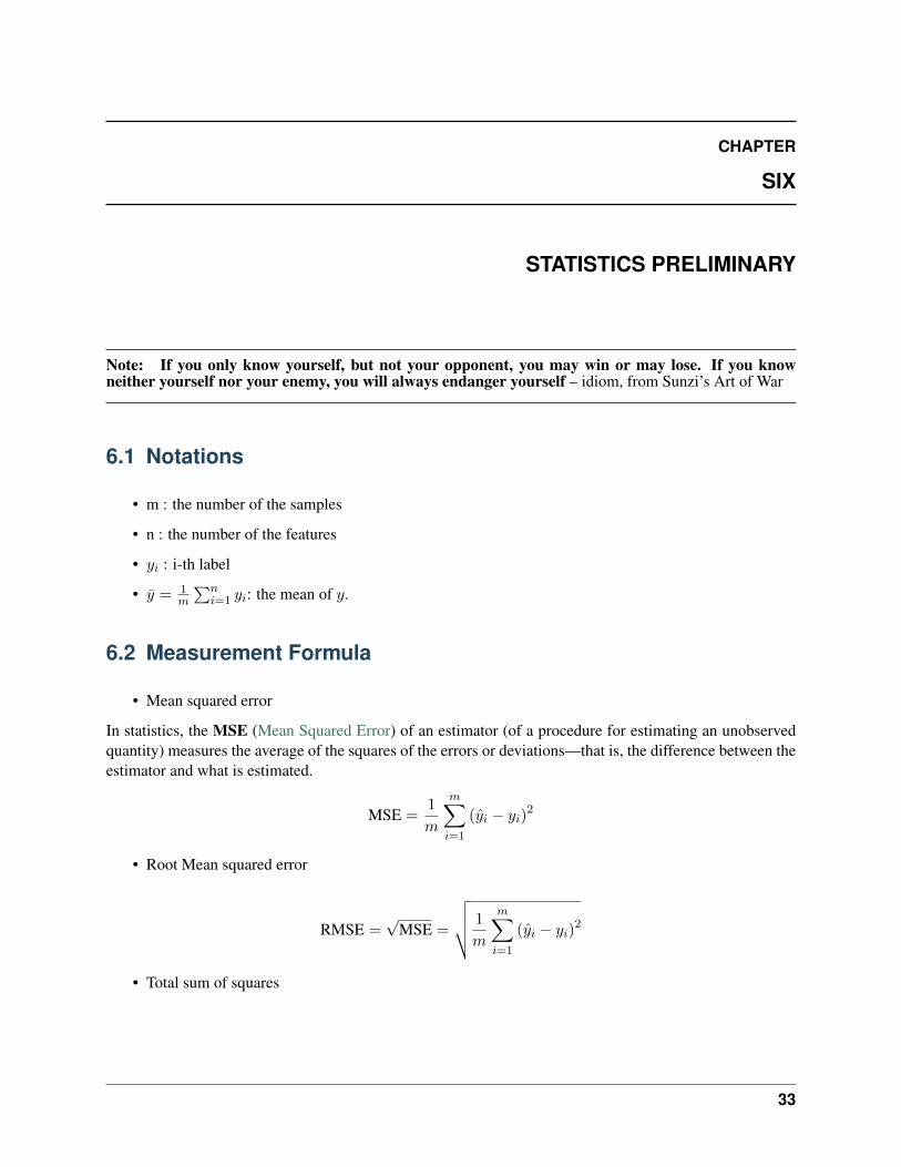
6.2 Measurement Formula
• Mean squared error
In statistics, the MSE (Mean Squared Error) of an estimator (of a procedure for estimating an unobservedquantity) measures the average of the squares of the errors or deviations—that is, the difference between theestimator and what is estimated.
MSE =1
𝑚
𝑚∑︁𝑖=1
(𝑦𝑖 − 𝑦𝑖)2
• Root Mean squared error
RMSE =√
MSE =
⎯⎸⎸⎷ 1
𝑚
𝑚∑︁𝑖=1
(𝑦𝑖 − 𝑦𝑖)2
• Total sum of squares
33
Learning Apache Spark with Python, Release v1.0
In statistical data analysis the TSS (Total Sum of Squares) is a quantity that appears as part of a standard wayof presenting results of such analyses. It is defined as being the sum, over all observations, of the squareddifferences of each observation from the overall mean.
TSS =𝑚∑︁𝑖=1
(𝑦𝑖 − 𝑦)2
• Residual Sum of Squares
RSS =1
𝑚
𝑚∑︁𝑖=1
(𝑦𝑖 − 𝑦𝑖)2
• Coefficient of determination 𝑅2
𝑅2 := 1 − RSSTSS
.
6.3 Statistical Tests
6.3.1 Correlational Test
• Pearson correlation: Tests for the strength of the association between two continuous variables.
• Spearman correlation: Tests for the strength of the association between two ordinal variables (doesnot rely on the assumption of normal distributed data).
• Chi-square: Tests for the strength of the association between two categorical variables.
6.3.2 Comparison of Means test
• Paired T-test: Tests for difference between two related variables.
• Independent T-test: Tests for difference between two independent variables.
• ANOVA: Tests the difference between group means after any other variance in the outcome variableis accounted for.
6.3.3 Non-parametric Test
• Wilcoxon rank-sum test: Tests for difference between two independent variables - takes into accountmagnitude and direction of difference.
• Wilcoxon sign-rank test: Tests for difference between two related variables - takes into account mag-nitude and direction of difference.
• Sign test: Tests if two related variables are different – ignores magnitude of change, only takes intoaccount direction.
34 Chapter 6. Statistics Preliminary
CHAPTER
SEVEN
DATA EXPLORATION
Note: A journey of a thousand miles begins with a single step – idiom, from Laozi.
I wouldn’t say that understanding your dataset is the most difficult thing in data science, but it is reallyimportant and time-consuming. Data Exploration is about describing the data by means of statistical andvisualization techniques. We explore data in order to understand the features and bring important featuresto our models.
7.1 Univariate Analysis
In mathematics, univariate refers to an expression, equation, function or polynomial of only one variable.“Uni” means “one”, so in other words your data has only one variable. So you do not need to deal with thecauses or relationships in this step. Univariate analysis takes data, summarizes that variables (attributes) oneby one and finds patterns in the data.
There are many ways that can describe patterns found in univariate data include central tendency (mean,mode and median) and dispersion: range, variance, maximum, minimum, quartiles (including the interquar-tile range), coefficient of variation and standard deviation. You also have several options for visualizing anddescribing data with univariate data. Such as frequency Distribution Tables, bar Charts,histograms, frequency Polygons, pie Charts.
The variable could be either categorical or numerical, I will demostrate the different statistical and visuliza-tion techniques to investigate each type of the variable.
• The Jupyter notebook can be download from Data Exploration.
• The data can be downloaf from German Credit.
7.1.1 Numerical Variables
• Describe
The desctibe function in pandas and spark will give us most of the statistical results, such as min,median, max, quartiles and standard deviation. With the help of the user defined function,you can get even more statistical results.
35
Learning Apache Spark with Python, Release v1.0
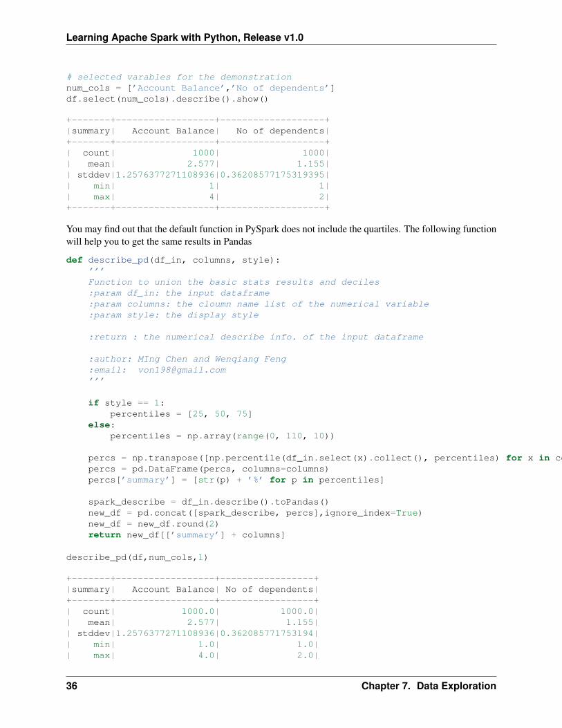
# selected varables for the demonstrationnum_cols = [’Account Balance’,’No of dependents’]df.select(num_cols).describe().show()
+-------+------------------+-------------------+|summary| Account Balance| No of dependents|+-------+------------------+-------------------+| count| 1000| 1000|| mean| 2.577| 1.155|| stddev|1.2576377271108936|0.36208577175319395|| min| 1| 1|| max| 4| 2|+-------+------------------+-------------------+
You may find out that the default function in PySpark does not include the quartiles. The following functionwill help you to get the same results in Pandas
def describe_pd(df_in, columns, style):’’’Function to union the basic stats results and deciles:param df_in: the input dataframe:param columns: the cloumn name list of the numerical variable:param style: the display style
:return : the numerical describe info. of the input dataframe
:author: MIng Chen and Wenqiang Feng:email: [email protected]’’’
if style == 1:percentiles = [25, 50, 75]
else:percentiles = np.array(range(0, 110, 10))
percs = np.transpose([np.percentile(df_in.select(x).collect(), percentiles) for x in columns])percs = pd.DataFrame(percs, columns=columns)percs[’summary’] = [str(p) + ’%’ for p in percentiles]
spark_describe = df_in.describe().toPandas()new_df = pd.concat([spark_describe, percs],ignore_index=True)new_df = new_df.round(2)return new_df[[’summary’] + columns]
describe_pd(df,num_cols,1)
+-------+------------------+-----------------+|summary| Account Balance| No of dependents|+-------+------------------+-----------------+| count| 1000.0| 1000.0|| mean| 2.577| 1.155|| stddev|1.2576377271108936|0.362085771753194|| min| 1.0| 1.0|| max| 4.0| 2.0|
36 Chapter 7. Data Exploration
Learning Apache Spark with Python, Release v1.0
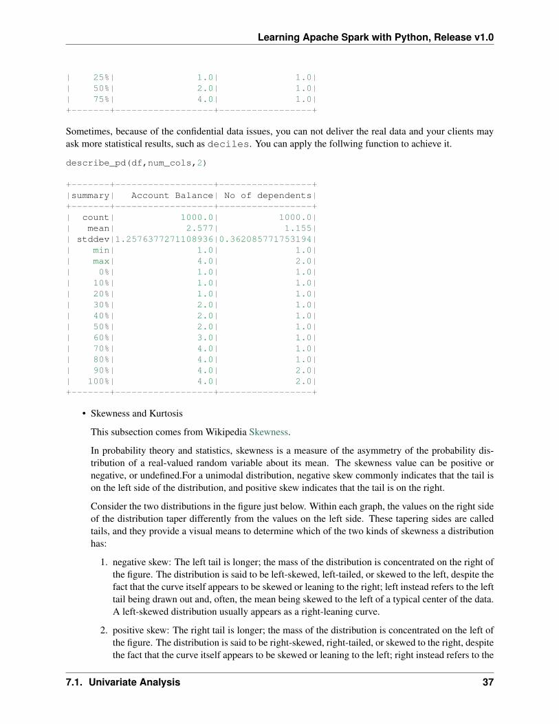
| 25%| 1.0| 1.0|| 50%| 2.0| 1.0|| 75%| 4.0| 1.0|+-------+------------------+-----------------+
Sometimes, because of the confidential data issues, you can not deliver the real data and your clients mayask more statistical results, such as deciles. You can apply the follwing function to achieve it.
describe_pd(df,num_cols,2)
+-------+------------------+-----------------+|summary| Account Balance| No of dependents|+-------+------------------+-----------------+| count| 1000.0| 1000.0|| mean| 2.577| 1.155|| stddev|1.2576377271108936|0.362085771753194|| min| 1.0| 1.0|| max| 4.0| 2.0|| 0%| 1.0| 1.0|| 10%| 1.0| 1.0|| 20%| 1.0| 1.0|| 30%| 2.0| 1.0|| 40%| 2.0| 1.0|| 50%| 2.0| 1.0|| 60%| 3.0| 1.0|| 70%| 4.0| 1.0|| 80%| 4.0| 1.0|| 90%| 4.0| 2.0|| 100%| 4.0| 2.0|+-------+------------------+-----------------+
• Skewness and Kurtosis
This subsection comes from Wikipedia Skewness.
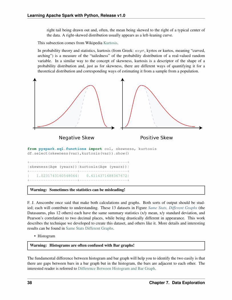
In probability theory and statistics, skewness is a measure of the asymmetry of the probability dis-tribution of a real-valued random variable about its mean. The skewness value can be positive ornegative, or undefined.For a unimodal distribution, negative skew commonly indicates that the tail ison the left side of the distribution, and positive skew indicates that the tail is on the right.
Consider the two distributions in the figure just below. Within each graph, the values on the right sideof the distribution taper differently from the values on the left side. These tapering sides are calledtails, and they provide a visual means to determine which of the two kinds of skewness a distributionhas:
1. negative skew: The left tail is longer; the mass of the distribution is concentrated on the right ofthe figure. The distribution is said to be left-skewed, left-tailed, or skewed to the left, despite thefact that the curve itself appears to be skewed or leaning to the right; left instead refers to the lefttail being drawn out and, often, the mean being skewed to the left of a typical center of the data.A left-skewed distribution usually appears as a right-leaning curve.
2. positive skew: The right tail is longer; the mass of the distribution is concentrated on the left ofthe figure. The distribution is said to be right-skewed, right-tailed, or skewed to the right, despitethe fact that the curve itself appears to be skewed or leaning to the left; right instead refers to the
7.1. Univariate Analysis 37
Learning Apache Spark with Python, Release v1.0
right tail being drawn out and, often, the mean being skewed to the right of a typical center ofthe data. A right-skewed distribution usually appears as a left-leaning curve.
This subsection comes from Wikipedia Kurtosis.
In probability theory and statistics, kurtosis (from Greek: 𝜅𝜐𝜌𝜏 , kyrtos or kurtos, meaning “curved,arching”) is a measure of the “tailedness” of the probability distribution of a real-valued randomvariable. In a similar way to the concept of skewness, kurtosis is a descriptor of the shape of aprobability distribution and, just as for skewness, there are different ways of quantifying it for atheoretical distribution and corresponding ways of estimating it from a sample from a population.
from pyspark.sql.functions import col, skewness, kurtosisdf.select(skewness(var),kurtosis(var)).show()
+---------------------+---------------------+|skewness(Age (years))|kurtosis(Age (years))|+---------------------+---------------------+| 1.0231743160548064| 0.6114371688367672|+---------------------+---------------------+
Warning: Sometimes the statistics can be misleading!
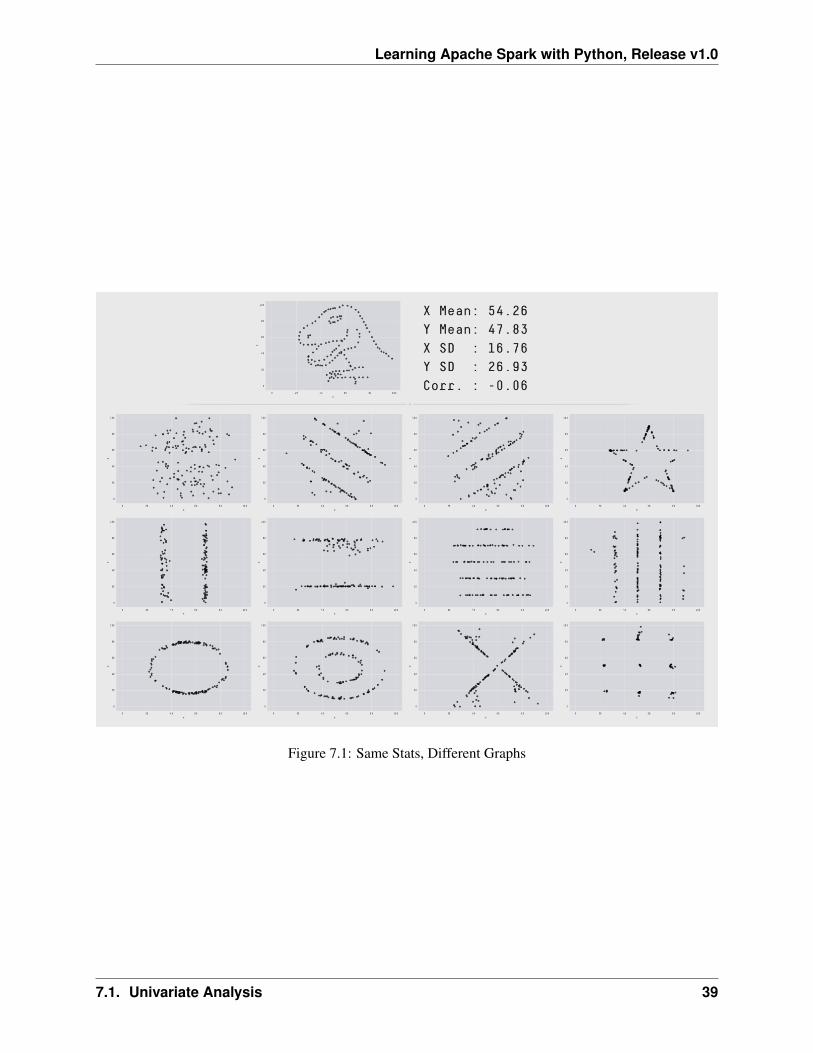
F. J. Anscombe once said that make both calculations and graphs. Both sorts of output should be stud-ied; each will contribute to understanding. These 13 datasets in Figure Same Stats, Different Graphs (theDatasaurus, plus 12 others) each have the same summary statistics (x/y mean, x/y standard deviation, andPearson’s correlation) to two decimal places, while being drastically different in appearance. This workdescribes the technique we developed to create this dataset, and others like it. More details and interestingresults can be found in Same Stats Different Graphs.
• Histogram
Warning: Histograms are often confused with Bar graphs!
The fundamental difference between histogram and bar graph will help you to identify the two easily is thatthere are gaps between bars in a bar graph but in the histogram, the bars are adjacent to each other. Theinterested reader is referred to Difference Between Histogram and Bar Graph.
38 Chapter 7. Data Exploration
Learning Apache Spark with Python, Release v1.0
Figure 7.1: Same Stats, Different Graphs
7.1. Univariate Analysis 39
Learning Apache Spark with Python, Release v1.0
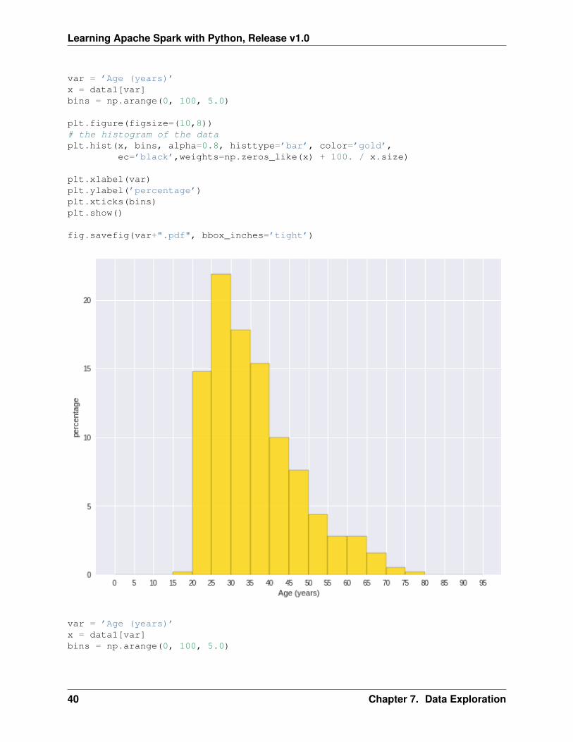
var = ’Age (years)’x = data1[var]bins = np.arange(0, 100, 5.0)
plt.figure(figsize=(10,8))# the histogram of the dataplt.hist(x, bins, alpha=0.8, histtype=’bar’, color=’gold’,
ec=’black’,weights=np.zeros_like(x) + 100. / x.size)
plt.xlabel(var)plt.ylabel(’percentage’)plt.xticks(bins)plt.show()
fig.savefig(var+".pdf", bbox_inches=’tight’)
var = ’Age (years)’x = data1[var]bins = np.arange(0, 100, 5.0)
40 Chapter 7. Data Exploration
Learning Apache Spark with Python, Release v1.0
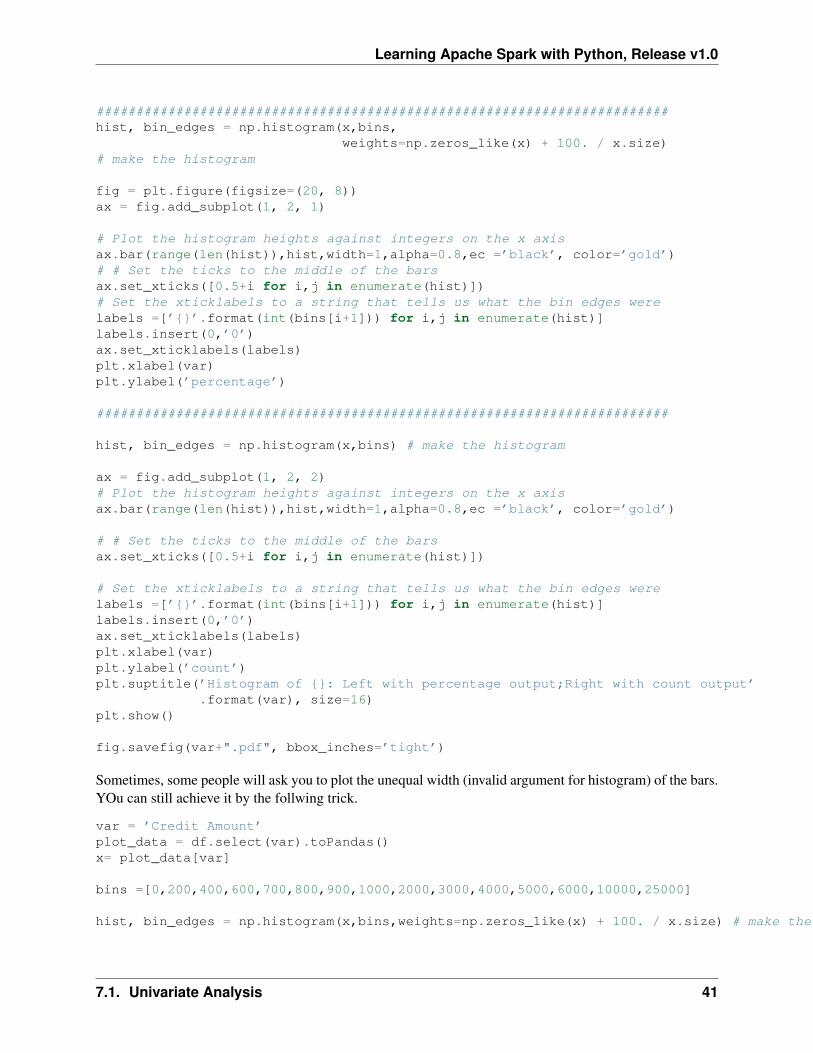
########################################################################hist, bin_edges = np.histogram(x,bins,
weights=np.zeros_like(x) + 100. / x.size)# make the histogram
fig = plt.figure(figsize=(20, 8))ax = fig.add_subplot(1, 2, 1)
# Plot the histogram heights against integers on the x axisax.bar(range(len(hist)),hist,width=1,alpha=0.8,ec =’black’, color=’gold’)# # Set the ticks to the middle of the barsax.set_xticks([0.5+i for i,j in enumerate(hist)])# Set the xticklabels to a string that tells us what the bin edges werelabels =[’{}’.format(int(bins[i+1])) for i,j in enumerate(hist)]labels.insert(0,’0’)ax.set_xticklabels(labels)plt.xlabel(var)plt.ylabel(’percentage’)
########################################################################
hist, bin_edges = np.histogram(x,bins) # make the histogram
ax = fig.add_subplot(1, 2, 2)# Plot the histogram heights against integers on the x axisax.bar(range(len(hist)),hist,width=1,alpha=0.8,ec =’black’, color=’gold’)
# # Set the ticks to the middle of the barsax.set_xticks([0.5+i for i,j in enumerate(hist)])
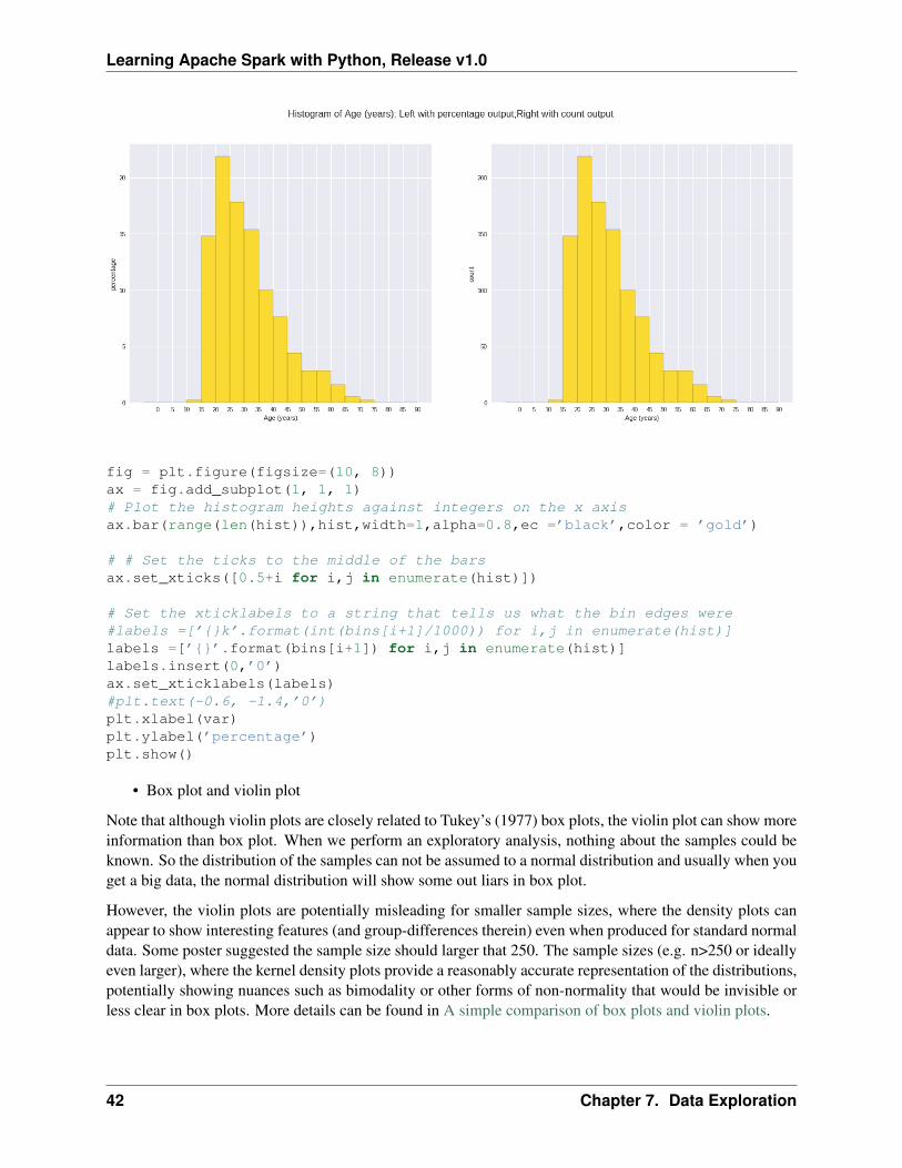
# Set the xticklabels to a string that tells us what the bin edges werelabels =[’{}’.format(int(bins[i+1])) for i,j in enumerate(hist)]labels.insert(0,’0’)ax.set_xticklabels(labels)plt.xlabel(var)plt.ylabel(’count’)plt.suptitle(’Histogram of {}: Left with percentage output;Right with count output’
.format(var), size=16)plt.show()
fig.savefig(var+".pdf", bbox_inches=’tight’)
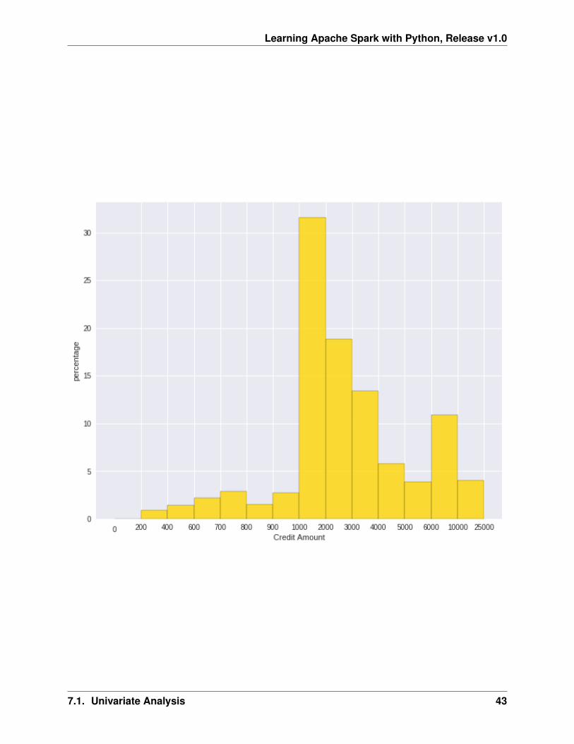
Sometimes, some people will ask you to plot the unequal width (invalid argument for histogram) of the bars.YOu can still achieve it by the follwing trick.
var = ’Credit Amount’plot_data = df.select(var).toPandas()x= plot_data[var]
bins =[0,200,400,600,700,800,900,1000,2000,3000,4000,5000,6000,10000,25000]
hist, bin_edges = np.histogram(x,bins,weights=np.zeros_like(x) + 100. / x.size) # make the histogram
7.1. Univariate Analysis 41
Learning Apache Spark with Python, Release v1.0
fig = plt.figure(figsize=(10, 8))ax = fig.add_subplot(1, 1, 1)# Plot the histogram heights against integers on the x axisax.bar(range(len(hist)),hist,width=1,alpha=0.8,ec =’black’,color = ’gold’)
# # Set the ticks to the middle of the barsax.set_xticks([0.5+i for i,j in enumerate(hist)])
# Set the xticklabels to a string that tells us what the bin edges were#labels =[’{}k’.format(int(bins[i+1]/1000)) for i,j in enumerate(hist)]labels =[’{}’.format(bins[i+1]) for i,j in enumerate(hist)]labels.insert(0,’0’)ax.set_xticklabels(labels)#plt.text(-0.6, -1.4,’0’)plt.xlabel(var)plt.ylabel(’percentage’)plt.show()
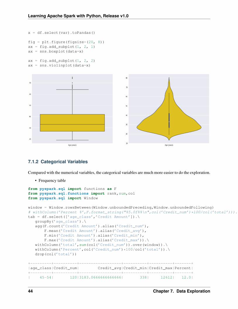
• Box plot and violin plot
Note that although violin plots are closely related to Tukey’s (1977) box plots, the violin plot can show moreinformation than box plot. When we perform an exploratory analysis, nothing about the samples could beknown. So the distribution of the samples can not be assumed to a normal distribution and usually when youget a big data, the normal distribution will show some out liars in box plot.
However, the violin plots are potentially misleading for smaller sample sizes, where the density plots canappear to show interesting features (and group-differences therein) even when produced for standard normaldata. Some poster suggested the sample size should larger that 250. The sample sizes (e.g. n>250 or ideallyeven larger), where the kernel density plots provide a reasonably accurate representation of the distributions,potentially showing nuances such as bimodality or other forms of non-normality that would be invisible orless clear in box plots. More details can be found in A simple comparison of box plots and violin plots.
42 Chapter 7. Data Exploration
Learning Apache Spark with Python, Release v1.0
7.1. Univariate Analysis 43
Learning Apache Spark with Python, Release v1.0
x = df.select(var).toPandas()
fig = plt.figure(figsize=(20, 8))ax = fig.add_subplot(1, 2, 1)ax = sns.boxplot(data=x)
ax = fig.add_subplot(1, 2, 2)ax = sns.violinplot(data=x)
7.1.2 Categorical Variables
Compared with the numerical variables, the categorical variables are much more easier to do the exploration.
• Frequency table
from pyspark.sql import functions as Ffrom pyspark.sql.functions import rank,sum,colfrom pyspark.sql import Window
window = Window.rowsBetween(Window.unboundedPreceding,Window.unboundedFollowing)# withColumn(’Percent %’,F.format_string("%5.0f%%\n",col(’Credit_num’)*100/col(’total’))).\tab = df.select([’age_class’,’Credit Amount’]).\
groupBy(’age_class’).\agg(F.count(’Credit Amount’).alias(’Credit_num’),
F.mean(’Credit Amount’).alias(’Credit_avg’),F.min(’Credit Amount’).alias(’Credit_min’),F.max(’Credit Amount’).alias(’Credit_max’)).\
withColumn(’total’,sum(col(’Credit_num’)).over(window)).\withColumn(’Percent’,col(’Credit_num’)*100/col(’total’)).\drop(col(’total’))
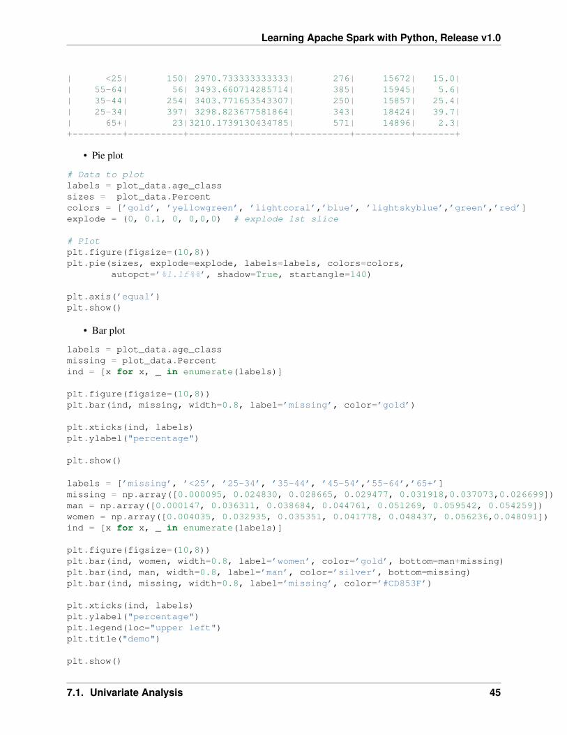
+---------+----------+------------------+----------+----------+-------+|age_class|Credit_num| Credit_avg|Credit_min|Credit_max|Percent|+---------+----------+------------------+----------+----------+-------+| 45-54| 120|3183.0666666666666| 338| 12612| 12.0|
44 Chapter 7. Data Exploration
Learning Apache Spark with Python, Release v1.0
| <25| 150| 2970.733333333333| 276| 15672| 15.0|| 55-64| 56| 3493.660714285714| 385| 15945| 5.6|| 35-44| 254| 3403.771653543307| 250| 15857| 25.4|| 25-34| 397| 3298.823677581864| 343| 18424| 39.7|| 65+| 23|3210.1739130434785| 571| 14896| 2.3|+---------+----------+------------------+----------+----------+-------+
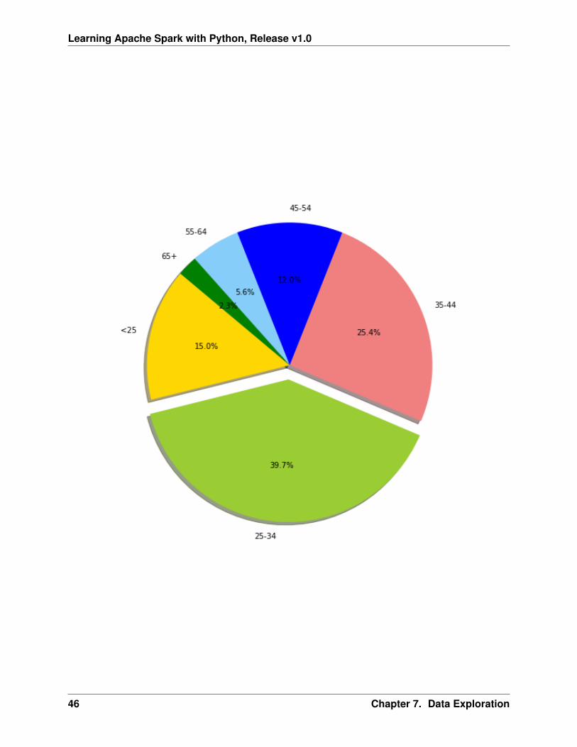
• Pie plot
# Data to plotlabels = plot_data.age_classsizes = plot_data.Percentcolors = [’gold’, ’yellowgreen’, ’lightcoral’,’blue’, ’lightskyblue’,’green’,’red’]explode = (0, 0.1, 0, 0,0,0) # explode 1st slice
# Plotplt.figure(figsize=(10,8))plt.pie(sizes, explode=explode, labels=labels, colors=colors,
autopct=’%1.1f%%’, shadow=True, startangle=140)
plt.axis(’equal’)plt.show()
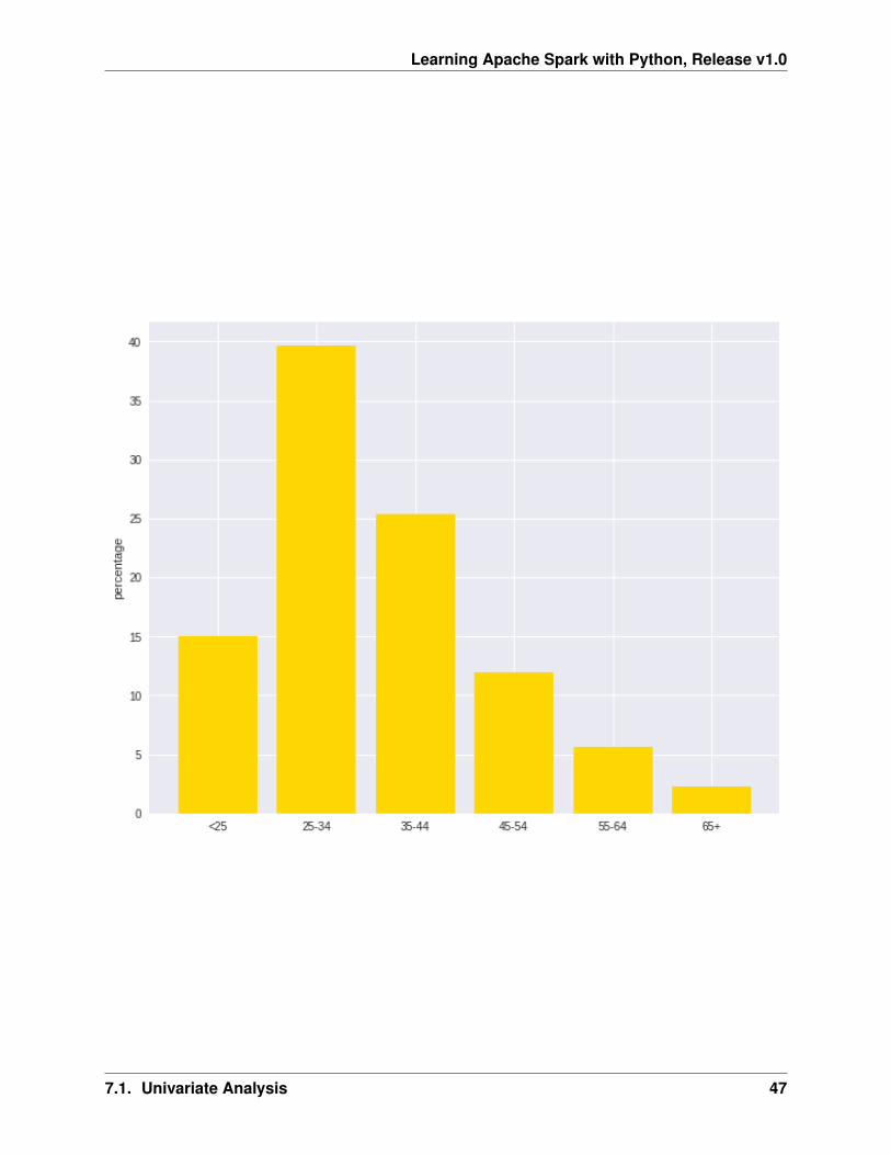
• Bar plot
labels = plot_data.age_classmissing = plot_data.Percentind = [x for x, _ in enumerate(labels)]
plt.figure(figsize=(10,8))plt.bar(ind, missing, width=0.8, label=’missing’, color=’gold’)
plt.xticks(ind, labels)plt.ylabel("percentage")
plt.show()
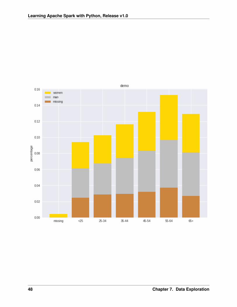
labels = [’missing’, ’<25’, ’25-34’, ’35-44’, ’45-54’,’55-64’,’65+’]missing = np.array([0.000095, 0.024830, 0.028665, 0.029477, 0.031918,0.037073,0.026699])man = np.array([0.000147, 0.036311, 0.038684, 0.044761, 0.051269, 0.059542, 0.054259])women = np.array([0.004035, 0.032935, 0.035351, 0.041778, 0.048437, 0.056236,0.048091])ind = [x for x, _ in enumerate(labels)]
plt.figure(figsize=(10,8))plt.bar(ind, women, width=0.8, label=’women’, color=’gold’, bottom=man+missing)plt.bar(ind, man, width=0.8, label=’man’, color=’silver’, bottom=missing)plt.bar(ind, missing, width=0.8, label=’missing’, color=’#CD853F’)
plt.xticks(ind, labels)plt.ylabel("percentage")plt.legend(loc="upper left")plt.title("demo")
plt.show()
7.1. Univariate Analysis 45
Learning Apache Spark with Python, Release v1.0
46 Chapter 7. Data Exploration
Learning Apache Spark with Python, Release v1.0
7.1. Univariate Analysis 47
Learning Apache Spark with Python, Release v1.0
48 Chapter 7. Data Exploration
Learning Apache Spark with Python, Release v1.0
7.2 Multivariate Analysis
In this section, I will only demostrate the bivariate analysis. Since the multivariate analysis is the generationof the bivariate.
7.2.1 Numerical V.S. Numerical
• Correlation matrix
from pyspark.mllib.stat import Statisticsimport pandas as pd
corr_data = df.select(num_cols)
col_names = corr_data.columnsfeatures = corr_data.rdd.map(lambda row: row[0:])corr_mat=Statistics.corr(features, method="pearson")corr_df = pd.DataFrame(corr_mat)corr_df.index, corr_df.columns = col_names, col_names
print(corr_df.to_string())
+--------------------+--------------------+| Account Balance| No of dependents|+--------------------+--------------------+| 1.0|-0.01414542650320914||-0.01414542650320914| 1.0|+--------------------+--------------------+
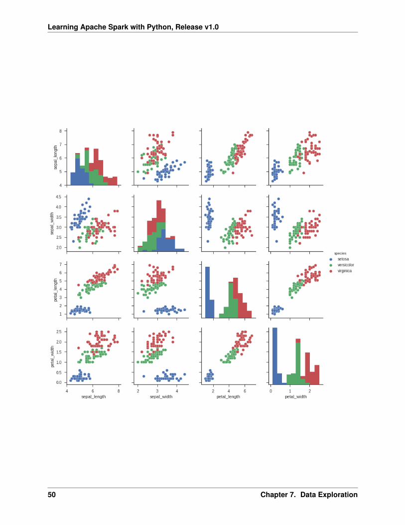
• Scatter Plot
import seaborn as snssns.set(style="ticks")
df = sns.load_dataset("iris")sns.pairplot(df, hue="species")plt.show()
7.2.2 Categorical V.S. Categorical
• Pearson’s Chi-squared test
Warning: pyspark.ml.stat is only available in Spark 2.4.0.
from pyspark.ml.linalg import Vectorsfrom pyspark.ml.stat import ChiSquareTest
data = [(0.0, Vectors.dense(0.5, 10.0)),(0.0, Vectors.dense(1.5, 20.0)),
7.2. Multivariate Analysis 49
Learning Apache Spark with Python, Release v1.0
50 Chapter 7. Data Exploration
Learning Apache Spark with Python, Release v1.0
(1.0, Vectors.dense(1.5, 30.0)),(0.0, Vectors.dense(3.5, 30.0)),(0.0, Vectors.dense(3.5, 40.0)),(1.0, Vectors.dense(3.5, 40.0))]
df = spark.createDataFrame(data, ["label", "features"])
r = ChiSquareTest.test(df, "features", "label").head()print("pValues: " + str(r.pValues))print("degreesOfFreedom: " + str(r.degreesOfFreedom))print("statistics: " + str(r.statistics))
pValues: [0.687289278791,0.682270330336]degreesOfFreedom: [2, 3]statistics: [0.75,1.5]
• Cross table
df.stat.crosstab("age_class", "Occupation").show()
+--------------------+---+---+---+---+|age_class_Occupation| 1| 2| 3| 4|+--------------------+---+---+---+---+| <25| 4| 34|108| 4|| 55-64| 1| 15| 31| 9|| 25-34| 7| 61|269| 60|| 35-44| 4| 58|143| 49|| 65+| 5| 3| 6| 9|| 45-54| 1| 29| 73| 17|+--------------------+---+---+---+---+
• Stacked plot
labels = [’missing’, ’<25’, ’25-34’, ’35-44’, ’45-54’,’55-64’,’65+’]missing = np.array([0.000095, 0.024830, 0.028665, 0.029477, 0.031918,0.037073,0.026699])man = np.array([0.000147, 0.036311, 0.038684, 0.044761, 0.051269, 0.059542, 0.054259])women = np.array([0.004035, 0.032935, 0.035351, 0.041778, 0.048437, 0.056236,0.048091])ind = [x for x, _ in enumerate(labels)]
plt.figure(figsize=(10,8))plt.bar(ind, women, width=0.8, label=’women’, color=’gold’, bottom=man+missing)plt.bar(ind, man, width=0.8, label=’man’, color=’silver’, bottom=missing)plt.bar(ind, missing, width=0.8, label=’missing’, color=’#CD853F’)
plt.xticks(ind, labels)plt.ylabel("percentage")plt.legend(loc="upper left")plt.title("demo")
plt.show()
7.2.3 Numerical V.S. Categorical
7.2. Multivariate Analysis 51

Learning Apache Spark with Python, Release v1.0
52 Chapter 7. Data Exploration
CHAPTER
EIGHT
REGRESSION
Note: A journey of a thousand miles begins with a single step – old Chinese proverb
In statistical modeling, regression analysis focuses on investigating the relationship between a dependentvariable and one or more independent variables. Wikipedia Regression analysis
In data mining, Regression is a model to represent the relationship between the value of lable ( or target,it is numerical variable) and on one or more features (or predictors they can be numerical and categoricalvariables).
8.1 Linear Regression
8.1.1 Introduction
Given that a data set {𝑥𝑖1, . . . , 𝑥𝑖𝑛, 𝑦𝑖}𝑚𝑖=1 which contains n features (variables) and m samples (data points),in simple linear regression model for modeling 𝑚 data points with one independent variable: 𝑥𝑖1, the formulais given by:
𝑦𝑖 = 𝛽0 + 𝛽1𝑥𝑖1,where, 𝑖 = 1, · · ·𝑚.
In matrix notation, the data set is written as X = [X1, · · · ,X𝑛] with X𝑖 = {𝑥·𝑖}𝑛𝑖=1, y = {𝑦𝑖}𝑚𝑖=1 and𝛽⊤ = {𝛽𝑖}𝑚𝑖=1. Then the normal equations are written as
y = X𝛽.
8.1.2 How to solve it?
1. Direct Methods (For more information please refer to my Prelim Notes for Numerical Analysis)
• For squared or rectangular matrices
– Singular Value Decomposition
53
Learning Apache Spark with Python, Release v1.0
– Gram-Schmidt orthogonalization
– QR Decomposition
• For squared matrices
– LU Decomposition
– Cholesky Decomposition
– Regular Splittings
2. Iterative Methods
• Stationary cases iterative method
– Jacobi Method
– Gauss-Seidel Method
– Richardson Method
– Successive Over Relaxation (SOR) Method
• Dynamic cases iterative method
– Chebyshev iterative Method
– Minimal residuals Method
– Minimal correction iterative method
– Steepest Descent Method
– Conjugate Gradients Method
8.1.3 Demo
• The Jupyter notebook can be download from Linear Regression which was implemented without usingPipeline.
• The Jupyter notebook can be download from Linear Regression with Pipeline which was implementedwith using Pipeline.
• I will only present the code with pipeline style in the following.
• For more details about the parameters, please visit Linear Regression API .
1. Set up spark context and SparkSession
from pyspark.sql import SparkSession
spark = SparkSession \.builder \.appName("Python Spark regression example") \.config("spark.some.config.option", "some-value") \.getOrCreate()
2. Load dataset
54 Chapter 8. Regression
Learning Apache Spark with Python, Release v1.0
df = spark.read.format(’com.databricks.spark.csv’).\options(header=’true’, \inferschema=’true’).\
load("../data/Advertising.csv",header=True);
check the data set
df.show(5,True)df.printSchema()
Then you will get
+-----+-----+---------+-----+| TV|Radio|Newspaper|Sales|+-----+-----+---------+-----+|230.1| 37.8| 69.2| 22.1|| 44.5| 39.3| 45.1| 10.4|| 17.2| 45.9| 69.3| 9.3||151.5| 41.3| 58.5| 18.5||180.8| 10.8| 58.4| 12.9|+-----+-----+---------+-----+only showing top 5 rows
root|-- TV: double (nullable = true)|-- Radio: double (nullable = true)|-- Newspaper: double (nullable = true)|-- Sales: double (nullable = true)
You can also get the Statistical resutls from the data frame (Unfortunately, it only works for numerical).
df.describe().show()
Then you will get
+-------+-----------------+------------------+------------------+------------------+|summary| TV| Radio| Newspaper| Sales|+-------+-----------------+------------------+------------------+------------------+| count| 200| 200| 200| 200|| mean| 147.0425|23.264000000000024|30.553999999999995|14.022500000000003|| stddev|85.85423631490805|14.846809176168728| 21.77862083852283| 5.217456565710477|| min| 0.7| 0.0| 0.3| 1.6|| max| 296.4| 49.6| 114.0| 27.0|+-------+-----------------+------------------+------------------+------------------+
3. Convert the data to dense vector (features and label)
from pyspark.sql import Rowfrom pyspark.ml.linalg import Vectors
# I provide two ways to build the features and labels
# method 1 (good for small feature):#def transData(row):# return Row(label=row["Sales"],
8.1. Linear Regression 55
Learning Apache Spark with Python, Release v1.0
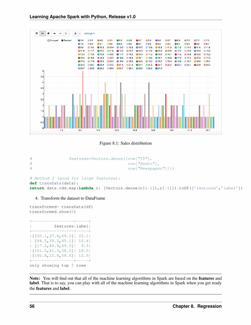
Figure 8.1: Sales distribution
# features=Vectors.dense([row["TV"],# row["Radio"],# row["Newspaper"]]))
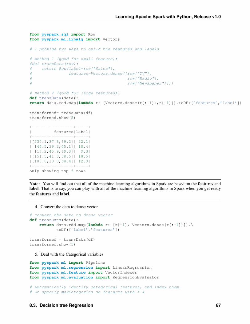
# Method 2 (good for large features):def transData(data):return data.rdd.map(lambda r: [Vectors.dense(r[:-1]),r[-1]]).toDF([’features’,’label’])
4. Transform the dataset to DataFrame
transformed= transData(df)transformed.show(5)
+-----------------+-----+| features|label|+-----------------+-----+|[230.1,37.8,69.2]| 22.1|| [44.5,39.3,45.1]| 10.4|| [17.2,45.9,69.3]| 9.3||[151.5,41.3,58.5]| 18.5||[180.8,10.8,58.4]| 12.9|+-----------------+-----+only showing top 5 rows
Note: You will find out that all of the machine learning algorithms in Spark are based on the features andlabel. That is to say, you can play with all of the machine learning algorithms in Spark when you get readythe features and label.
56 Chapter 8. Regression
Learning Apache Spark with Python, Release v1.0
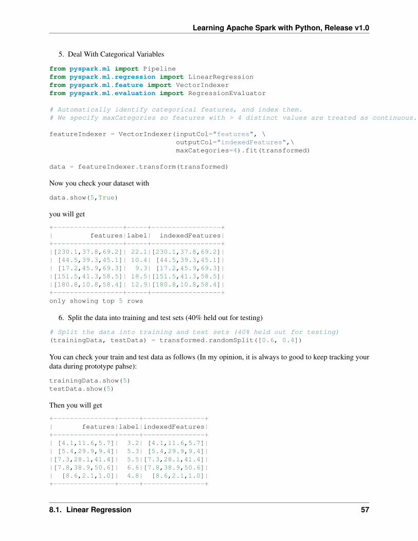
5. Deal With Categorical Variables
from pyspark.ml import Pipelinefrom pyspark.ml.regression import LinearRegressionfrom pyspark.ml.feature import VectorIndexerfrom pyspark.ml.evaluation import RegressionEvaluator
# Automatically identify categorical features, and index them.# We specify maxCategories so features with > 4 distinct values are treated as continuous.
featureIndexer = VectorIndexer(inputCol="features", \outputCol="indexedFeatures",\maxCategories=4).fit(transformed)
data = featureIndexer.transform(transformed)
Now you check your dataset with
data.show(5,True)
you will get
+-----------------+-----+-----------------+| features|label| indexedFeatures|+-----------------+-----+-----------------+|[230.1,37.8,69.2]| 22.1|[230.1,37.8,69.2]|| [44.5,39.3,45.1]| 10.4| [44.5,39.3,45.1]|| [17.2,45.9,69.3]| 9.3| [17.2,45.9,69.3]||[151.5,41.3,58.5]| 18.5|[151.5,41.3,58.5]||[180.8,10.8,58.4]| 12.9|[180.8,10.8,58.4]|+-----------------+-----+-----------------+only showing top 5 rows
6. Split the data into training and test sets (40% held out for testing)
# Split the data into training and test sets (40% held out for testing)(trainingData, testData) = transformed.randomSplit([0.6, 0.4])
You can check your train and test data as follows (In my opinion, it is always to good to keep tracking yourdata during prototype pahse):
trainingData.show(5)testData.show(5)
Then you will get
+---------------+-----+---------------+| features|label|indexedFeatures|+---------------+-----+---------------+| [4.1,11.6,5.7]| 3.2| [4.1,11.6,5.7]|| [5.4,29.9,9.4]| 5.3| [5.4,29.9,9.4]||[7.3,28.1,41.4]| 5.5|[7.3,28.1,41.4]||[7.8,38.9,50.6]| 6.6|[7.8,38.9,50.6]|| [8.6,2.1,1.0]| 4.8| [8.6,2.1,1.0]|+---------------+-----+---------------+
8.1. Linear Regression 57
Learning Apache Spark with Python, Release v1.0
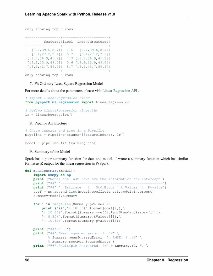
only showing top 5 rows
+----------------+-----+----------------+| features|label| indexedFeatures|+----------------+-----+----------------+| [0.7,39.6,8.7]| 1.6| [0.7,39.6,8.7]|| [8.4,27.2,2.1]| 5.7| [8.4,27.2,2.1]||[11.7,36.9,45.2]| 7.3|[11.7,36.9,45.2]||[13.2,15.9,49.6]| 5.6|[13.2,15.9,49.6]||[16.9,43.7,89.4]| 8.7|[16.9,43.7,89.4]|+----------------+-----+----------------+only showing top 5 rows
7. Fit Ordinary Least Square Regression Model
For more details about the parameters, please visit Linear Regression API .
# Import LinearRegression classfrom pyspark.ml.regression import LinearRegression
# Define LinearRegression algorithmlr = LinearRegression()
8. Pipeline Architecture
# Chain indexer and tree in a Pipelinepipeline = Pipeline(stages=[featureIndexer, lr])
model = pipeline.fit(trainingData)
9. Summary of the Model
Spark has a poor summary function for data and model. I wrote a summary function which has similarformat as R output for the linear regression in PySpark.
def modelsummary(model):import numpy as npprint ("Note: the last rows are the information for Intercept")print ("##","-------------------------------------------------")print ("##"," Estimate | Std.Error | t Values | P-value")coef = np.append(list(model.coefficients),model.intercept)Summary=model.summary
for i in range(len(Summary.pValues)):print ("##",’{:10.6f}’.format(coef[i]),\’{:10.6f}’.format(Summary.coefficientStandardErrors[i]),\’{:8.3f}’.format(Summary.tValues[i]),\’{:10.6f}’.format(Summary.pValues[i]))
print ("##",’---’)print ("##","Mean squared error: % .6f" \
% Summary.meanSquaredError, ", RMSE: % .6f" \% Summary.rootMeanSquaredError )
print ("##","Multiple R-squared: %f" % Summary.r2, ", \
58 Chapter 8. Regression
Learning Apache Spark with Python, Release v1.0
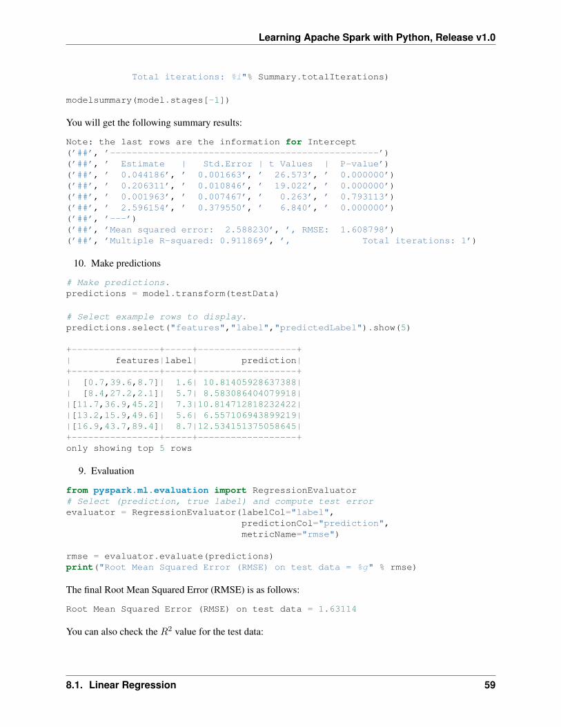
Total iterations: %i"% Summary.totalIterations)
modelsummary(model.stages[-1])
You will get the following summary results:
Note: the last rows are the information for Intercept(’##’, ’-------------------------------------------------’)(’##’, ’ Estimate | Std.Error | t Values | P-value’)(’##’, ’ 0.044186’, ’ 0.001663’, ’ 26.573’, ’ 0.000000’)(’##’, ’ 0.206311’, ’ 0.010846’, ’ 19.022’, ’ 0.000000’)(’##’, ’ 0.001963’, ’ 0.007467’, ’ 0.263’, ’ 0.793113’)(’##’, ’ 2.596154’, ’ 0.379550’, ’ 6.840’, ’ 0.000000’)(’##’, ’---’)(’##’, ’Mean squared error: 2.588230’, ’, RMSE: 1.608798’)(’##’, ’Multiple R-squared: 0.911869’, ’, Total iterations: 1’)
10. Make predictions
# Make predictions.predictions = model.transform(testData)
# Select example rows to display.predictions.select("features","label","predictedLabel").show(5)
+----------------+-----+------------------+| features|label| prediction|+----------------+-----+------------------+| [0.7,39.6,8.7]| 1.6| 10.81405928637388|| [8.4,27.2,2.1]| 5.7| 8.583086404079918||[11.7,36.9,45.2]| 7.3|10.814712818232422||[13.2,15.9,49.6]| 5.6| 6.557106943899219||[16.9,43.7,89.4]| 8.7|12.534151375058645|+----------------+-----+------------------+only showing top 5 rows
9. Evaluation
from pyspark.ml.evaluation import RegressionEvaluator# Select (prediction, true label) and compute test errorevaluator = RegressionEvaluator(labelCol="label",
predictionCol="prediction",metricName="rmse")
rmse = evaluator.evaluate(predictions)print("Root Mean Squared Error (RMSE) on test data = %g" % rmse)
The final Root Mean Squared Error (RMSE) is as follows:
Root Mean Squared Error (RMSE) on test data = 1.63114
You can also check the 𝑅2 value for the test data:
8.1. Linear Regression 59
Learning Apache Spark with Python, Release v1.0
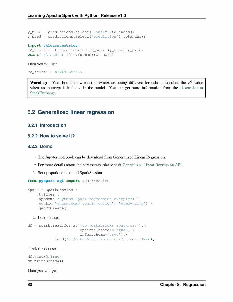
y_true = predictions.select("label").toPandas()y_pred = predictions.select("prediction").toPandas()
import sklearn.metricsr2_score = sklearn.metrics.r2_score(y_true, y_pred)print(’r2_score: {0}’.format(r2_score))
Then you will get
r2_score: 0.854486655585
Warning: You should know most softwares are using different formula to calculate the 𝑅2 valuewhen no intercept is included in the model. You can get more information from the disscussion atStackExchange.
8.2 Generalized linear regression
8.2.1 Introduction
8.2.2 How to solve it?
8.2.3 Demo
• The Jupyter notebook can be download from Generalized Linear Regression.
• For more details about the parameters, please visit Generalized Linear Regression API .
1. Set up spark context and SparkSession
from pyspark.sql import SparkSession
spark = SparkSession \.builder \.appName("Python Spark regression example") \.config("spark.some.config.option", "some-value") \.getOrCreate()
2. Load dataset
df = spark.read.format(’com.databricks.spark.csv’).\options(header=’true’, \inferschema=’true’).\
load("../data/Advertising.csv",header=True);
check the data set
df.show(5,True)df.printSchema()
Then you will get
60 Chapter 8. Regression
Learning Apache Spark with Python, Release v1.0
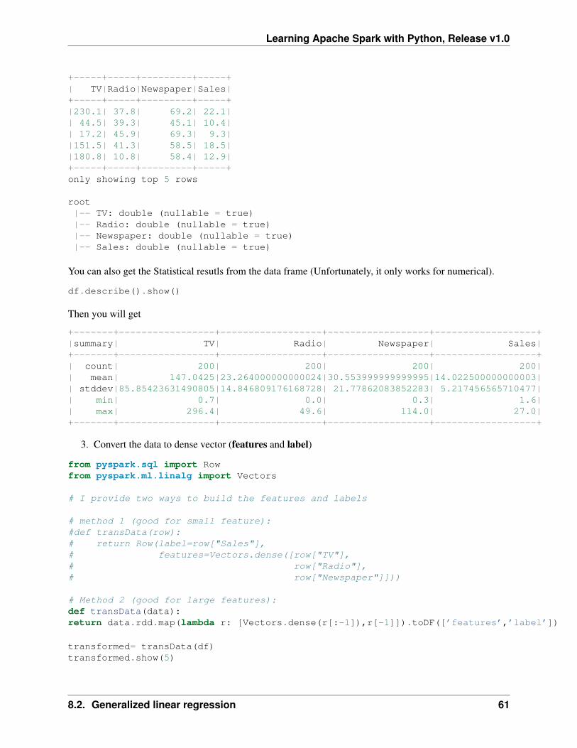
+-----+-----+---------+-----+| TV|Radio|Newspaper|Sales|+-----+-----+---------+-----+|230.1| 37.8| 69.2| 22.1|| 44.5| 39.3| 45.1| 10.4|| 17.2| 45.9| 69.3| 9.3||151.5| 41.3| 58.5| 18.5||180.8| 10.8| 58.4| 12.9|+-----+-----+---------+-----+only showing top 5 rows
root|-- TV: double (nullable = true)|-- Radio: double (nullable = true)|-- Newspaper: double (nullable = true)|-- Sales: double (nullable = true)
You can also get the Statistical resutls from the data frame (Unfortunately, it only works for numerical).
df.describe().show()
Then you will get
+-------+-----------------+------------------+------------------+------------------+|summary| TV| Radio| Newspaper| Sales|+-------+-----------------+------------------+------------------+------------------+| count| 200| 200| 200| 200|| mean| 147.0425|23.264000000000024|30.553999999999995|14.022500000000003|| stddev|85.85423631490805|14.846809176168728| 21.77862083852283| 5.217456565710477|| min| 0.7| 0.0| 0.3| 1.6|| max| 296.4| 49.6| 114.0| 27.0|+-------+-----------------+------------------+------------------+------------------+
3. Convert the data to dense vector (features and label)
from pyspark.sql import Rowfrom pyspark.ml.linalg import Vectors
# I provide two ways to build the features and labels
# method 1 (good for small feature):#def transData(row):# return Row(label=row["Sales"],# features=Vectors.dense([row["TV"],# row["Radio"],# row["Newspaper"]]))
# Method 2 (good for large features):def transData(data):return data.rdd.map(lambda r: [Vectors.dense(r[:-1]),r[-1]]).toDF([’features’,’label’])
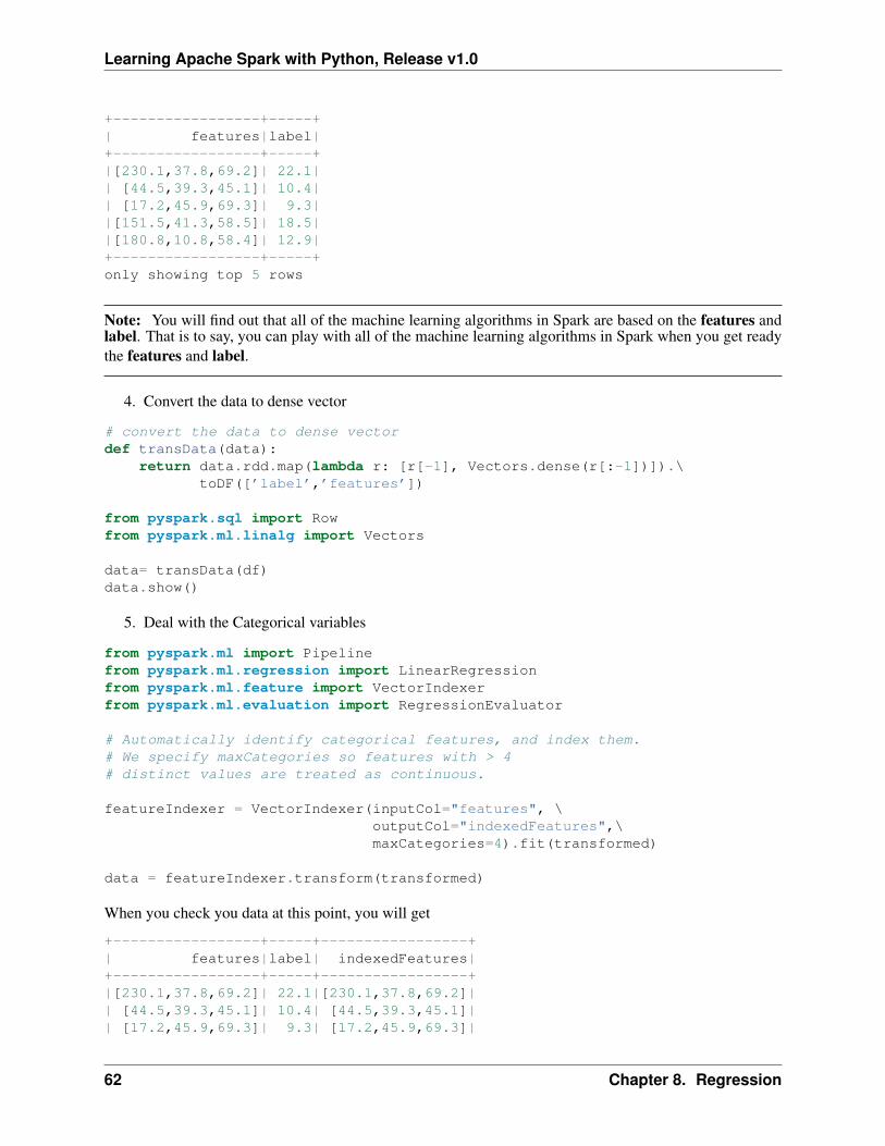
transformed= transData(df)transformed.show(5)
8.2. Generalized linear regression 61
Learning Apache Spark with Python, Release v1.0
+-----------------+-----+| features|label|+-----------------+-----+|[230.1,37.8,69.2]| 22.1|| [44.5,39.3,45.1]| 10.4|| [17.2,45.9,69.3]| 9.3||[151.5,41.3,58.5]| 18.5||[180.8,10.8,58.4]| 12.9|+-----------------+-----+only showing top 5 rows
Note: You will find out that all of the machine learning algorithms in Spark are based on the features andlabel. That is to say, you can play with all of the machine learning algorithms in Spark when you get readythe features and label.
4. Convert the data to dense vector
# convert the data to dense vectordef transData(data):
return data.rdd.map(lambda r: [r[-1], Vectors.dense(r[:-1])]).\toDF([’label’,’features’])
from pyspark.sql import Rowfrom pyspark.ml.linalg import Vectors
data= transData(df)data.show()
5. Deal with the Categorical variables
from pyspark.ml import Pipelinefrom pyspark.ml.regression import LinearRegressionfrom pyspark.ml.feature import VectorIndexerfrom pyspark.ml.evaluation import RegressionEvaluator
# Automatically identify categorical features, and index them.# We specify maxCategories so features with > 4# distinct values are treated as continuous.
featureIndexer = VectorIndexer(inputCol="features", \outputCol="indexedFeatures",\maxCategories=4).fit(transformed)
data = featureIndexer.transform(transformed)
When you check you data at this point, you will get
+-----------------+-----+-----------------+| features|label| indexedFeatures|+-----------------+-----+-----------------+|[230.1,37.8,69.2]| 22.1|[230.1,37.8,69.2]|| [44.5,39.3,45.1]| 10.4| [44.5,39.3,45.1]|| [17.2,45.9,69.3]| 9.3| [17.2,45.9,69.3]|
62 Chapter 8. Regression
Learning Apache Spark with Python, Release v1.0
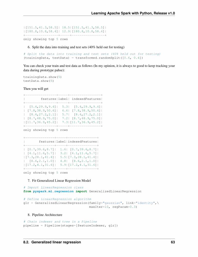
|[151.5,41.3,58.5]| 18.5|[151.5,41.3,58.5]||[180.8,10.8,58.4]| 12.9|[180.8,10.8,58.4]|+-----------------+-----+-----------------+only showing top 5 rows
6. Split the data into training and test sets (40% held out for testing)
# Split the data into training and test sets (40% held out for testing)(trainingData, testData) = transformed.randomSplit([0.6, 0.4])
You can check your train and test data as follows (In my opinion, it is always to good to keep tracking yourdata during prototype pahse):
trainingData.show(5)testData.show(5)
Then you will get
+----------------+-----+----------------+| features|label| indexedFeatures|+----------------+-----+----------------+| [5.4,29.9,9.4]| 5.3| [5.4,29.9,9.4]|| [7.8,38.9,50.6]| 6.6| [7.8,38.9,50.6]|| [8.4,27.2,2.1]| 5.7| [8.4,27.2,2.1]|| [8.7,48.9,75.0]| 7.2| [8.7,48.9,75.0]||[11.7,36.9,45.2]| 7.3|[11.7,36.9,45.2]|+----------------+-----+----------------+only showing top 5 rows
+---------------+-----+---------------+| features|label|indexedFeatures|+---------------+-----+---------------+| [0.7,39.6,8.7]| 1.6| [0.7,39.6,8.7]|| [4.1,11.6,5.7]| 3.2| [4.1,11.6,5.7]||[7.3,28.1,41.4]| 5.5|[7.3,28.1,41.4]|| [8.6,2.1,1.0]| 4.8| [8.6,2.1,1.0]||[17.2,4.1,31.6]| 5.9|[17.2,4.1,31.6]|+---------------+-----+---------------+only showing top 5 rows
7. Fit Generalized Linear Regression Model
# Import LinearRegression classfrom pyspark.ml.regression import GeneralizedLinearRegression
# Define LinearRegression algorithmglr = GeneralizedLinearRegression(family="gaussian", link="identity",\
maxIter=10, regParam=0.3)
8. Pipeline Architecture
# Chain indexer and tree in a Pipelinepipeline = Pipeline(stages=[featureIndexer, glr])
8.2. Generalized linear regression 63
Learning Apache Spark with Python, Release v1.0
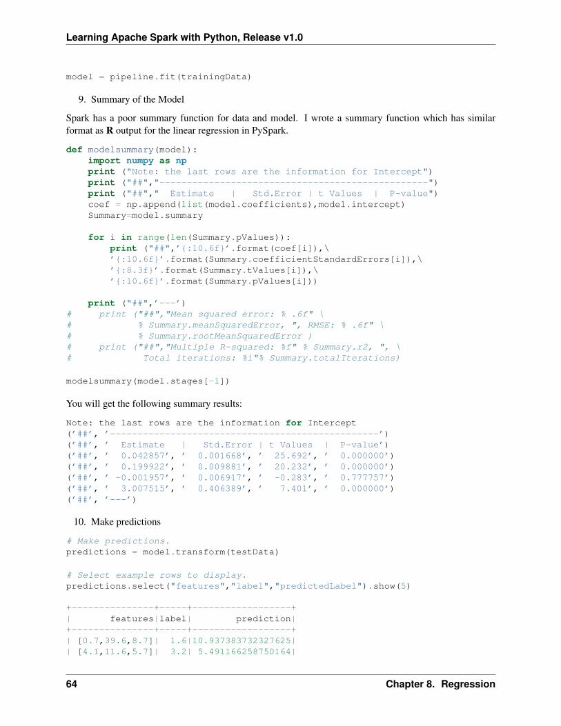
model = pipeline.fit(trainingData)
9. Summary of the Model
Spark has a poor summary function for data and model. I wrote a summary function which has similarformat as R output for the linear regression in PySpark.
def modelsummary(model):import numpy as npprint ("Note: the last rows are the information for Intercept")print ("##","-------------------------------------------------")print ("##"," Estimate | Std.Error | t Values | P-value")coef = np.append(list(model.coefficients),model.intercept)Summary=model.summary
for i in range(len(Summary.pValues)):print ("##",’{:10.6f}’.format(coef[i]),\’{:10.6f}’.format(Summary.coefficientStandardErrors[i]),\’{:8.3f}’.format(Summary.tValues[i]),\’{:10.6f}’.format(Summary.pValues[i]))
print ("##",’---’)# print ("##","Mean squared error: % .6f" \# % Summary.meanSquaredError, ", RMSE: % .6f" \# % Summary.rootMeanSquaredError )# print ("##","Multiple R-squared: %f" % Summary.r2, ", \# Total iterations: %i"% Summary.totalIterations)
modelsummary(model.stages[-1])
You will get the following summary results:
Note: the last rows are the information for Intercept(’##’, ’-------------------------------------------------’)(’##’, ’ Estimate | Std.Error | t Values | P-value’)(’##’, ’ 0.042857’, ’ 0.001668’, ’ 25.692’, ’ 0.000000’)(’##’, ’ 0.199922’, ’ 0.009881’, ’ 20.232’, ’ 0.000000’)(’##’, ’ -0.001957’, ’ 0.006917’, ’ -0.283’, ’ 0.777757’)(’##’, ’ 3.007515’, ’ 0.406389’, ’ 7.401’, ’ 0.000000’)(’##’, ’---’)
10. Make predictions
# Make predictions.predictions = model.transform(testData)
# Select example rows to display.predictions.select("features","label","predictedLabel").show(5)
+---------------+-----+------------------+| features|label| prediction|+---------------+-----+------------------+| [0.7,39.6,8.7]| 1.6|10.937383732327625|| [4.1,11.6,5.7]| 3.2| 5.491166258750164|
64 Chapter 8. Regression
Learning Apache Spark with Python, Release v1.0
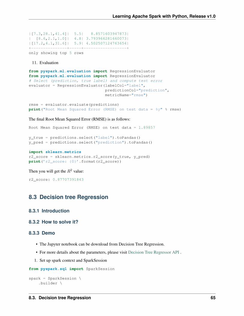
|[7.3,28.1,41.4]| 5.5| 8.8571603947873|| [8.6,2.1,1.0]| 4.8| 3.793966281660073||[17.2,4.1,31.6]| 5.9| 4.502507124763654|+---------------+-----+------------------+only showing top 5 rows
11. Evaluation
from pyspark.ml.evaluation import RegressionEvaluatorfrom pyspark.ml.evaluation import RegressionEvaluator# Select (prediction, true label) and compute test errorevaluator = RegressionEvaluator(labelCol="label",
predictionCol="prediction",metricName="rmse")
rmse = evaluator.evaluate(predictions)print("Root Mean Squared Error (RMSE) on test data = %g" % rmse)
The final Root Mean Squared Error (RMSE) is as follows:
Root Mean Squared Error (RMSE) on test data = 1.89857
y_true = predictions.select("label").toPandas()y_pred = predictions.select("prediction").toPandas()
import sklearn.metricsr2_score = sklearn.metrics.r2_score(y_true, y_pred)print(’r2_score: {0}’.format(r2_score))
Then you will get the 𝑅2 value:
r2_score: 0.87707391843
8.3 Decision tree Regression
8.3.1 Introduction
8.3.2 How to solve it?
8.3.3 Demo
• The Jupyter notebook can be download from Decision Tree Regression.
• For more details about the parameters, please visit Decision Tree Regressor API .
1. Set up spark context and SparkSession
from pyspark.sql import SparkSession
spark = SparkSession \.builder \
8.3. Decision tree Regression 65
Learning Apache Spark with Python, Release v1.0
.appName("Python Spark regression example") \
.config("spark.some.config.option", "some-value") \
.getOrCreate()
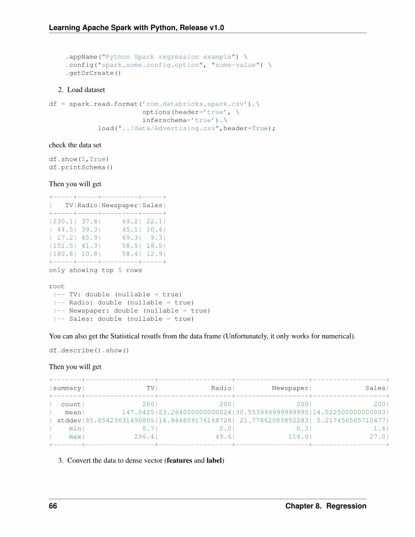
2. Load dataset
df = spark.read.format(’com.databricks.spark.csv’).\options(header=’true’, \inferschema=’true’).\
load("../data/Advertising.csv",header=True);
check the data set
df.show(5,True)df.printSchema()
Then you will get
+-----+-----+---------+-----+| TV|Radio|Newspaper|Sales|+-----+-----+---------+-----+|230.1| 37.8| 69.2| 22.1|| 44.5| 39.3| 45.1| 10.4|| 17.2| 45.9| 69.3| 9.3||151.5| 41.3| 58.5| 18.5||180.8| 10.8| 58.4| 12.9|+-----+-----+---------+-----+only showing top 5 rows
root|-- TV: double (nullable = true)|-- Radio: double (nullable = true)|-- Newspaper: double (nullable = true)|-- Sales: double (nullable = true)
You can also get the Statistical resutls from the data frame (Unfortunately, it only works for numerical).
df.describe().show()
Then you will get
+-------+-----------------+------------------+------------------+------------------+|summary| TV| Radio| Newspaper| Sales|+-------+-----------------+------------------+------------------+------------------+| count| 200| 200| 200| 200|| mean| 147.0425|23.264000000000024|30.553999999999995|14.022500000000003|| stddev|85.85423631490805|14.846809176168728| 21.77862083852283| 5.217456565710477|| min| 0.7| 0.0| 0.3| 1.6|| max| 296.4| 49.6| 114.0| 27.0|+-------+-----------------+------------------+------------------+------------------+
3. Convert the data to dense vector (features and label)
66 Chapter 8. Regression
Learning Apache Spark with Python, Release v1.0
from pyspark.sql import Rowfrom pyspark.ml.linalg import Vectors
# I provide two ways to build the features and labels
# method 1 (good for small feature):#def transData(row):# return Row(label=row["Sales"],# features=Vectors.dense([row["TV"],# row["Radio"],# row["Newspaper"]]))
# Method 2 (good for large features):def transData(data):return data.rdd.map(lambda r: [Vectors.dense(r[:-1]),r[-1]]).toDF([’features’,’label’])
transformed= transData(df)transformed.show(5)
+-----------------+-----+| features|label|+-----------------+-----+|[230.1,37.8,69.2]| 22.1|| [44.5,39.3,45.1]| 10.4|| [17.2,45.9,69.3]| 9.3||[151.5,41.3,58.5]| 18.5||[180.8,10.8,58.4]| 12.9|+-----------------+-----+only showing top 5 rows
Note: You will find out that all of the machine learning algorithms in Spark are based on the features andlabel. That is to say, you can play with all of the machine learning algorithms in Spark when you get readythe features and label.
4. Convert the data to dense vector
# convert the data to dense vectordef transData(data):
return data.rdd.map(lambda r: [r[-1], Vectors.dense(r[:-1])]).\toDF([’label’,’features’])
transformed = transData(df)transformed.show(5)
5. Deal with the Categorical variables
from pyspark.ml import Pipelinefrom pyspark.ml.regression import LinearRegressionfrom pyspark.ml.feature import VectorIndexerfrom pyspark.ml.evaluation import RegressionEvaluator
# Automatically identify categorical features, and index them.# We specify maxCategories so features with > 4
8.3. Decision tree Regression 67
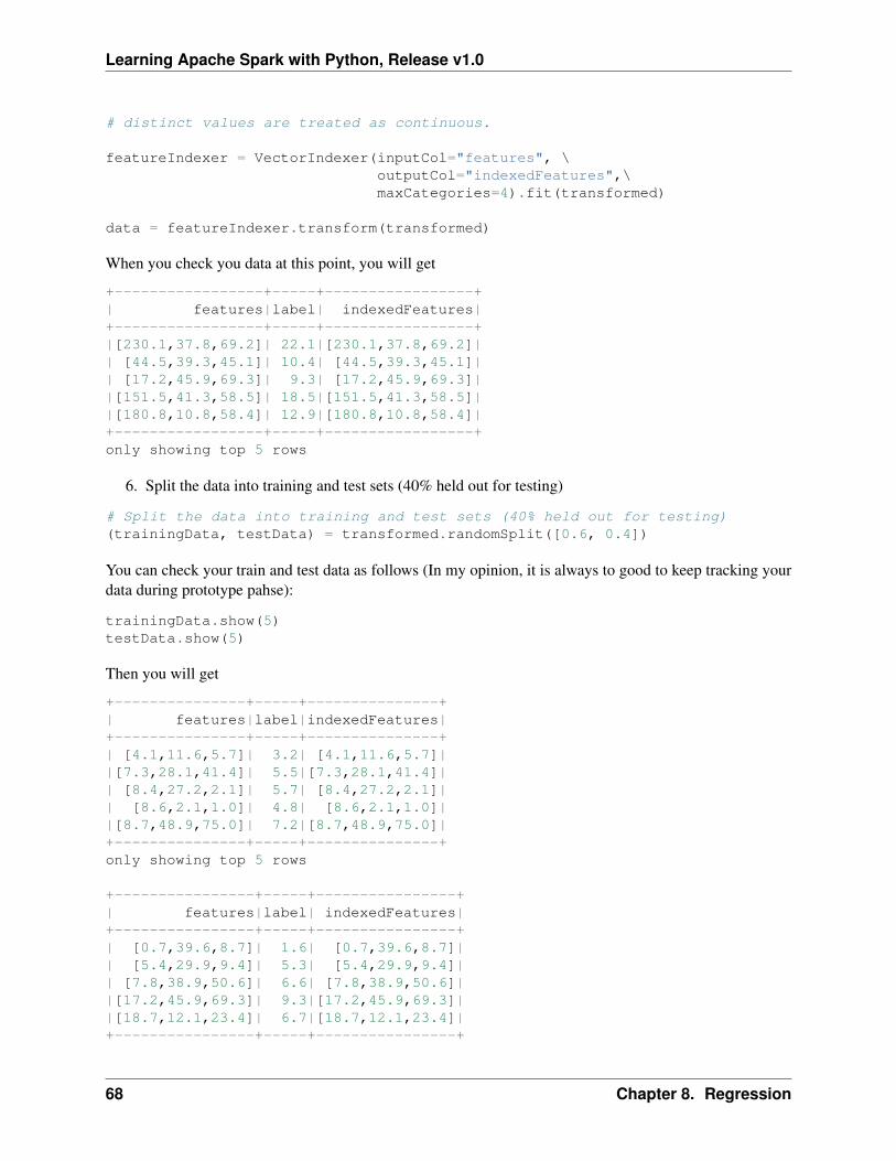
Learning Apache Spark with Python, Release v1.0
# distinct values are treated as continuous.
featureIndexer = VectorIndexer(inputCol="features", \outputCol="indexedFeatures",\maxCategories=4).fit(transformed)
data = featureIndexer.transform(transformed)
When you check you data at this point, you will get
+-----------------+-----+-----------------+| features|label| indexedFeatures|+-----------------+-----+-----------------+|[230.1,37.8,69.2]| 22.1|[230.1,37.8,69.2]|| [44.5,39.3,45.1]| 10.4| [44.5,39.3,45.1]|| [17.2,45.9,69.3]| 9.3| [17.2,45.9,69.3]||[151.5,41.3,58.5]| 18.5|[151.5,41.3,58.5]||[180.8,10.8,58.4]| 12.9|[180.8,10.8,58.4]|+-----------------+-----+-----------------+only showing top 5 rows
6. Split the data into training and test sets (40% held out for testing)
# Split the data into training and test sets (40% held out for testing)(trainingData, testData) = transformed.randomSplit([0.6, 0.4])
You can check your train and test data as follows (In my opinion, it is always to good to keep tracking yourdata during prototype pahse):
trainingData.show(5)testData.show(5)
Then you will get
+---------------+-----+---------------+| features|label|indexedFeatures|+---------------+-----+---------------+| [4.1,11.6,5.7]| 3.2| [4.1,11.6,5.7]||[7.3,28.1,41.4]| 5.5|[7.3,28.1,41.4]|| [8.4,27.2,2.1]| 5.7| [8.4,27.2,2.1]|| [8.6,2.1,1.0]| 4.8| [8.6,2.1,1.0]||[8.7,48.9,75.0]| 7.2|[8.7,48.9,75.0]|+---------------+-----+---------------+only showing top 5 rows
+----------------+-----+----------------+| features|label| indexedFeatures|+----------------+-----+----------------+| [0.7,39.6,8.7]| 1.6| [0.7,39.6,8.7]|| [5.4,29.9,9.4]| 5.3| [5.4,29.9,9.4]|| [7.8,38.9,50.6]| 6.6| [7.8,38.9,50.6]||[17.2,45.9,69.3]| 9.3|[17.2,45.9,69.3]||[18.7,12.1,23.4]| 6.7|[18.7,12.1,23.4]|+----------------+-----+----------------+
68 Chapter 8. Regression
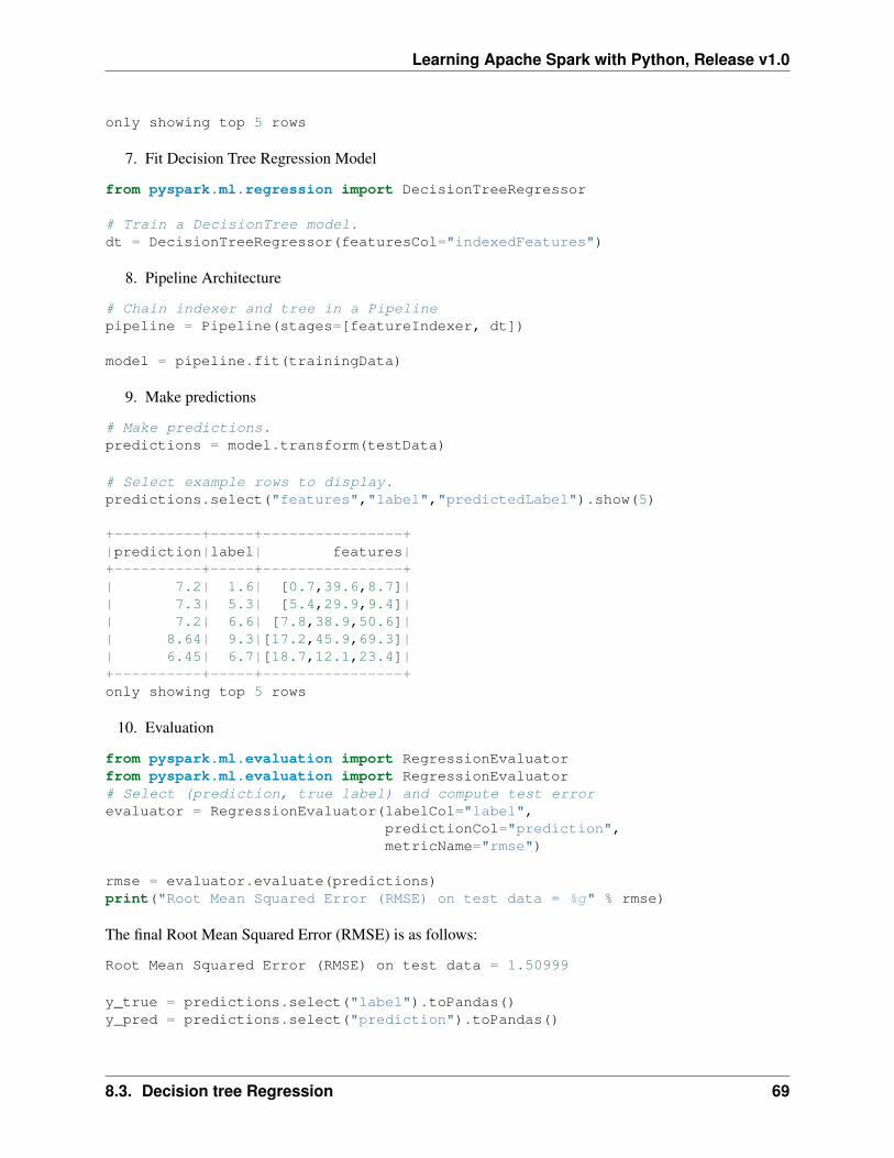
Learning Apache Spark with Python, Release v1.0
only showing top 5 rows
7. Fit Decision Tree Regression Model
from pyspark.ml.regression import DecisionTreeRegressor
# Train a DecisionTree model.dt = DecisionTreeRegressor(featuresCol="indexedFeatures")
8. Pipeline Architecture
# Chain indexer and tree in a Pipelinepipeline = Pipeline(stages=[featureIndexer, dt])
model = pipeline.fit(trainingData)
9. Make predictions
# Make predictions.predictions = model.transform(testData)
# Select example rows to display.predictions.select("features","label","predictedLabel").show(5)
+----------+-----+----------------+|prediction|label| features|+----------+-----+----------------+| 7.2| 1.6| [0.7,39.6,8.7]|| 7.3| 5.3| [5.4,29.9,9.4]|| 7.2| 6.6| [7.8,38.9,50.6]|| 8.64| 9.3|[17.2,45.9,69.3]|| 6.45| 6.7|[18.7,12.1,23.4]|+----------+-----+----------------+only showing top 5 rows
10. Evaluation
from pyspark.ml.evaluation import RegressionEvaluatorfrom pyspark.ml.evaluation import RegressionEvaluator# Select (prediction, true label) and compute test errorevaluator = RegressionEvaluator(labelCol="label",
predictionCol="prediction",metricName="rmse")
rmse = evaluator.evaluate(predictions)print("Root Mean Squared Error (RMSE) on test data = %g" % rmse)
The final Root Mean Squared Error (RMSE) is as follows:
Root Mean Squared Error (RMSE) on test data = 1.50999
y_true = predictions.select("label").toPandas()y_pred = predictions.select("prediction").toPandas()
8.3. Decision tree Regression 69
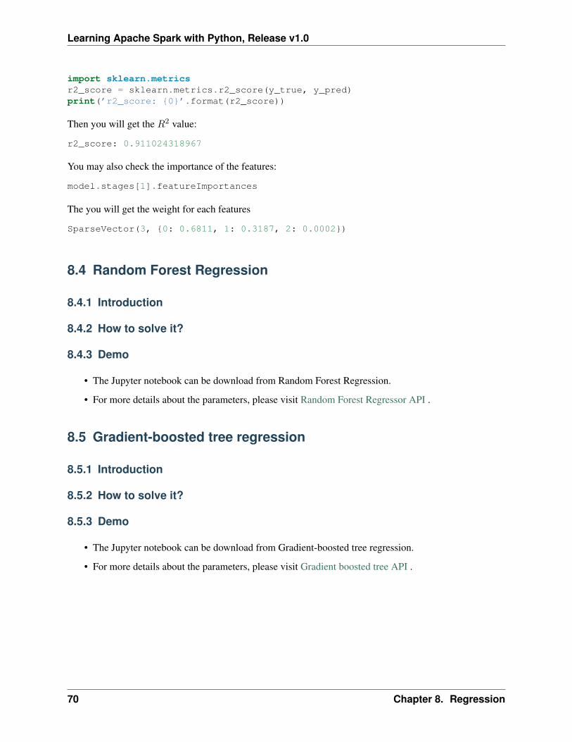
Learning Apache Spark with Python, Release v1.0
import sklearn.metricsr2_score = sklearn.metrics.r2_score(y_true, y_pred)print(’r2_score: {0}’.format(r2_score))
Then you will get the 𝑅2 value:
r2_score: 0.911024318967
You may also check the importance of the features:
model.stages[1].featureImportances
The you will get the weight for each features
SparseVector(3, {0: 0.6811, 1: 0.3187, 2: 0.0002})
8.4 Random Forest Regression
8.4.1 Introduction
8.4.2 How to solve it?
8.4.3 Demo
• The Jupyter notebook can be download from Random Forest Regression.
• For more details about the parameters, please visit Random Forest Regressor API .
8.5 Gradient-boosted tree regression
8.5.1 Introduction
8.5.2 How to solve it?
8.5.3 Demo
• The Jupyter notebook can be download from Gradient-boosted tree regression.
• For more details about the parameters, please visit Gradient boosted tree API .
70 Chapter 8. Regression
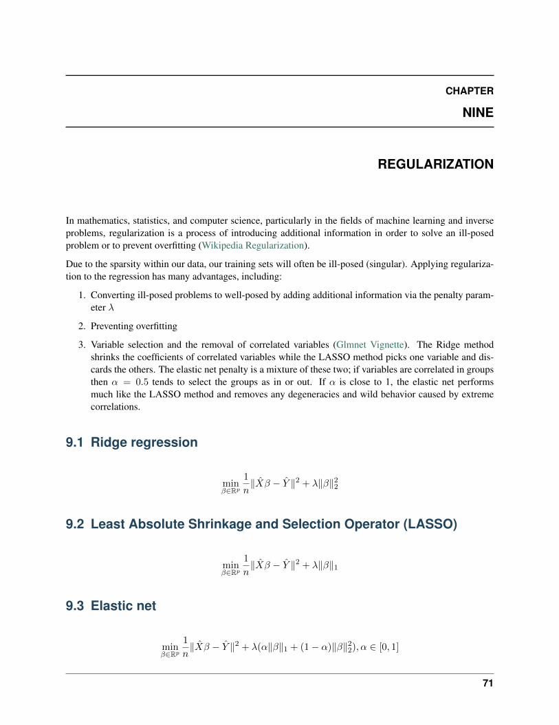
CHAPTER
NINE
REGULARIZATION
In mathematics, statistics, and computer science, particularly in the fields of machine learning and inverseproblems, regularization is a process of introducing additional information in order to solve an ill-posedproblem or to prevent overfitting (Wikipedia Regularization).
Due to the sparsity within our data, our training sets will often be ill-posed (singular). Applying regulariza-tion to the regression has many advantages, including:
1. Converting ill-posed problems to well-posed by adding additional information via the penalty param-eter 𝜆
2. Preventing overfitting
3. Variable selection and the removal of correlated variables (Glmnet Vignette). The Ridge methodshrinks the coefficients of correlated variables while the LASSO method picks one variable and dis-cards the others. The elastic net penalty is a mixture of these two; if variables are correlated in groupsthen 𝛼 = 0.5 tends to select the groups as in or out. If 𝛼 is close to 1, the elastic net performsmuch like the LASSO method and removes any degeneracies and wild behavior caused by extremecorrelations.
9.1 Ridge regression
min𝛽∈R𝑝
1
𝑛‖�̂�𝛽 − 𝑌 ‖2 + 𝜆‖𝛽‖22
9.2 Least Absolute Shrinkage and Selection Operator (LASSO)
min𝛽∈R𝑝
1
𝑛‖�̂�𝛽 − 𝑌 ‖2 + 𝜆‖𝛽‖1
9.3 Elastic net
min𝛽∈R𝑝
1
𝑛‖�̂�𝛽 − 𝑌 ‖2 + 𝜆(𝛼‖𝛽‖1 + (1 − 𝛼)‖𝛽‖22), 𝛼 ∈ [0, 1]
71

Learning Apache Spark with Python, Release v1.0
72 Chapter 9. Regularization
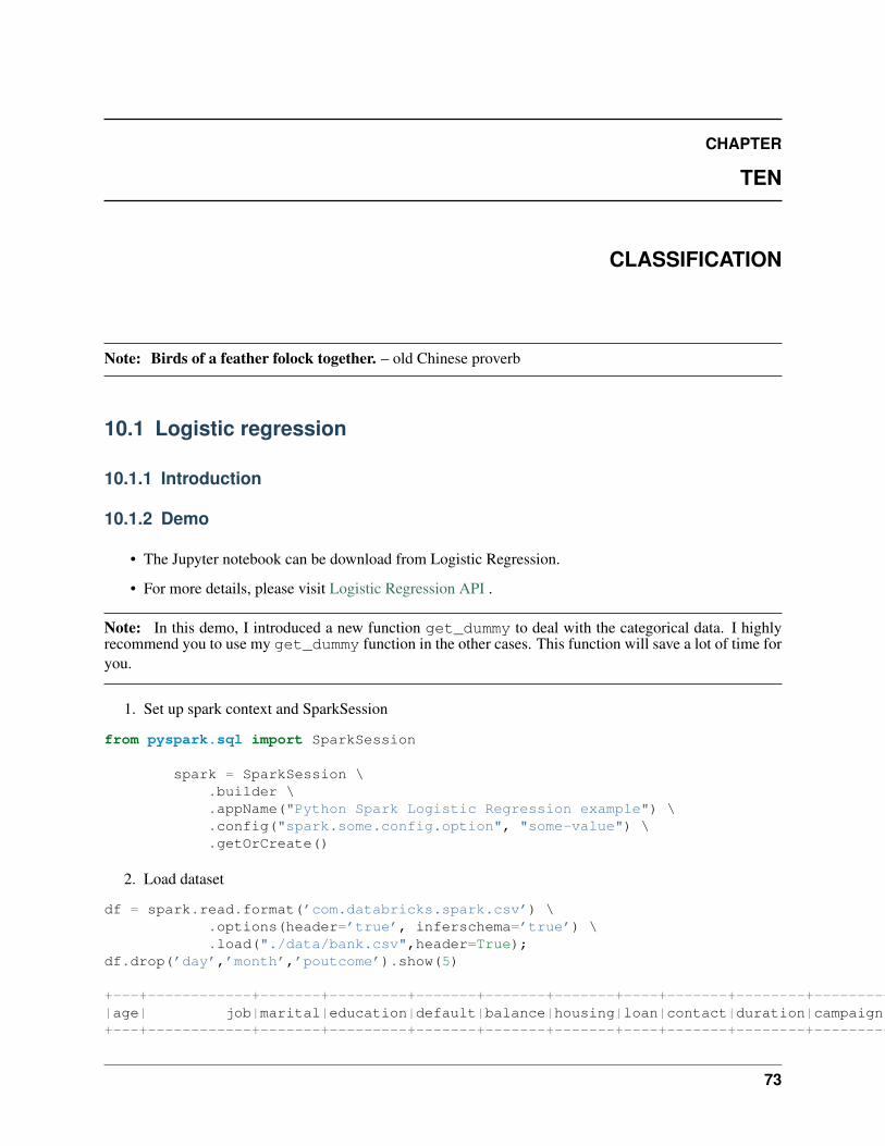
CHAPTER
TEN
CLASSIFICATION
Note: Birds of a feather folock together. – old Chinese proverb
10.1 Logistic regression
10.1.1 Introduction
10.1.2 Demo
• The Jupyter notebook can be download from Logistic Regression.
• For more details, please visit Logistic Regression API .
Note: In this demo, I introduced a new function get_dummy to deal with the categorical data. I highlyrecommend you to use my get_dummy function in the other cases. This function will save a lot of time foryou.
1. Set up spark context and SparkSession
from pyspark.sql import SparkSession
spark = SparkSession \.builder \.appName("Python Spark Logistic Regression example") \.config("spark.some.config.option", "some-value") \.getOrCreate()
2. Load dataset
df = spark.read.format(’com.databricks.spark.csv’) \.options(header=’true’, inferschema=’true’) \.load("./data/bank.csv",header=True);
df.drop(’day’,’month’,’poutcome’).show(5)
+---+------------+-------+---------+-------+-------+-------+----+-------+--------+--------+-----+--------+---+|age| job|marital|education|default|balance|housing|loan|contact|duration|campaign|pdays|previous| y|+---+------------+-------+---------+-------+-------+-------+----+-------+--------+--------+-----+--------+---+
73
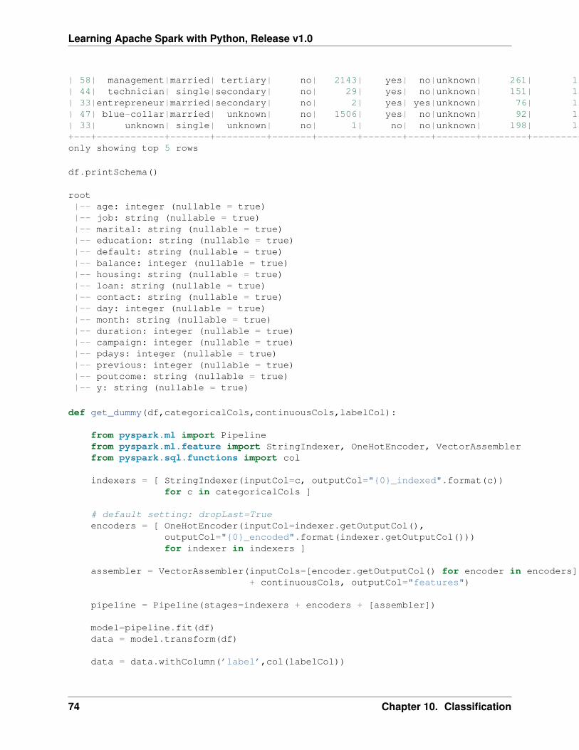
Learning Apache Spark with Python, Release v1.0
| 58| management|married| tertiary| no| 2143| yes| no|unknown| 261| 1| -1| 0| no|| 44| technician| single|secondary| no| 29| yes| no|unknown| 151| 1| -1| 0| no|| 33|entrepreneur|married|secondary| no| 2| yes| yes|unknown| 76| 1| -1| 0| no|| 47| blue-collar|married| unknown| no| 1506| yes| no|unknown| 92| 1| -1| 0| no|| 33| unknown| single| unknown| no| 1| no| no|unknown| 198| 1| -1| 0| no|+---+------------+-------+---------+-------+-------+-------+----+-------+--------+--------+-----+--------+---+only showing top 5 rows
df.printSchema()
root|-- age: integer (nullable = true)|-- job: string (nullable = true)|-- marital: string (nullable = true)|-- education: string (nullable = true)|-- default: string (nullable = true)|-- balance: integer (nullable = true)|-- housing: string (nullable = true)|-- loan: string (nullable = true)|-- contact: string (nullable = true)|-- day: integer (nullable = true)|-- month: string (nullable = true)|-- duration: integer (nullable = true)|-- campaign: integer (nullable = true)|-- pdays: integer (nullable = true)|-- previous: integer (nullable = true)|-- poutcome: string (nullable = true)|-- y: string (nullable = true)
def get_dummy(df,categoricalCols,continuousCols,labelCol):
from pyspark.ml import Pipelinefrom pyspark.ml.feature import StringIndexer, OneHotEncoder, VectorAssemblerfrom pyspark.sql.functions import col
indexers = [ StringIndexer(inputCol=c, outputCol="{0}_indexed".format(c))for c in categoricalCols ]
# default setting: dropLast=Trueencoders = [ OneHotEncoder(inputCol=indexer.getOutputCol(),
outputCol="{0}_encoded".format(indexer.getOutputCol()))for indexer in indexers ]
assembler = VectorAssembler(inputCols=[encoder.getOutputCol() for encoder in encoders]+ continuousCols, outputCol="features")
pipeline = Pipeline(stages=indexers + encoders + [assembler])
model=pipeline.fit(df)data = model.transform(df)
data = data.withColumn(’label’,col(labelCol))
74 Chapter 10. Classification
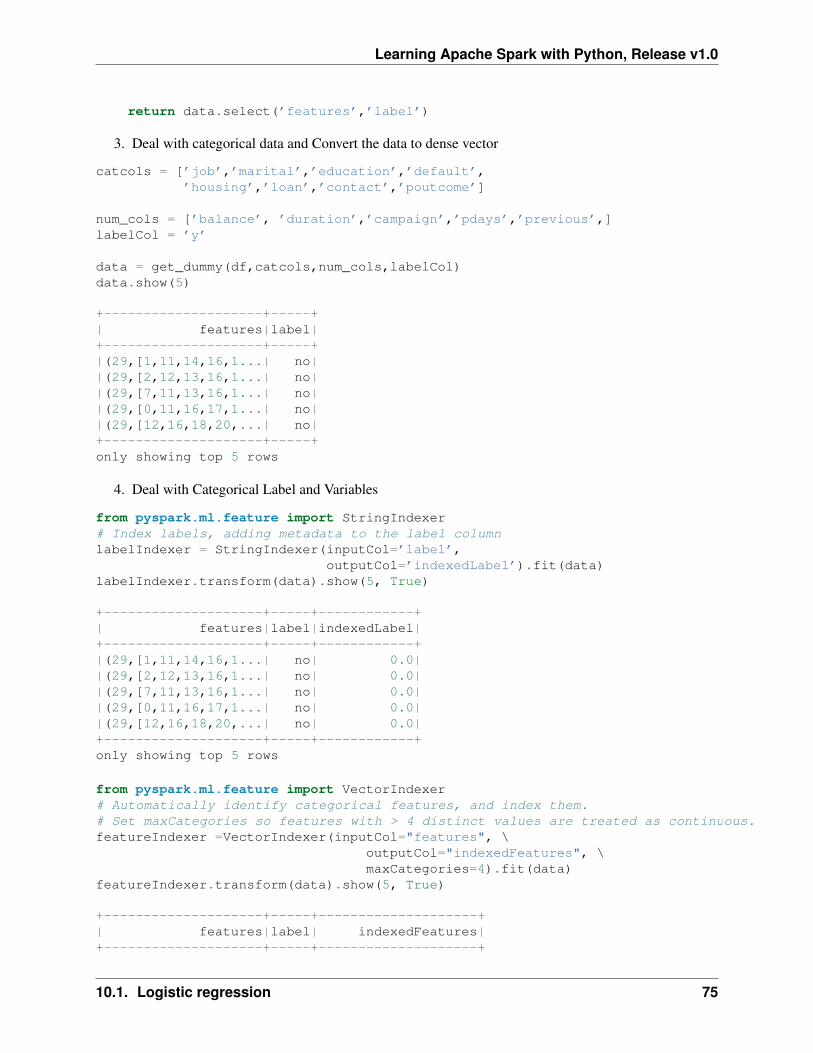
Learning Apache Spark with Python, Release v1.0
return data.select(’features’,’label’)
3. Deal with categorical data and Convert the data to dense vector
catcols = [’job’,’marital’,’education’,’default’,’housing’,’loan’,’contact’,’poutcome’]
num_cols = [’balance’, ’duration’,’campaign’,’pdays’,’previous’,]labelCol = ’y’
data = get_dummy(df,catcols,num_cols,labelCol)data.show(5)
+--------------------+-----+| features|label|+--------------------+-----+|(29,[1,11,14,16,1...| no||(29,[2,12,13,16,1...| no||(29,[7,11,13,16,1...| no||(29,[0,11,16,17,1...| no||(29,[12,16,18,20,...| no|+--------------------+-----+only showing top 5 rows
4. Deal with Categorical Label and Variables
from pyspark.ml.feature import StringIndexer# Index labels, adding metadata to the label columnlabelIndexer = StringIndexer(inputCol=’label’,
outputCol=’indexedLabel’).fit(data)labelIndexer.transform(data).show(5, True)
+--------------------+-----+------------+| features|label|indexedLabel|+--------------------+-----+------------+|(29,[1,11,14,16,1...| no| 0.0||(29,[2,12,13,16,1...| no| 0.0||(29,[7,11,13,16,1...| no| 0.0||(29,[0,11,16,17,1...| no| 0.0||(29,[12,16,18,20,...| no| 0.0|+--------------------+-----+------------+only showing top 5 rows
from pyspark.ml.feature import VectorIndexer# Automatically identify categorical features, and index them.# Set maxCategories so features with > 4 distinct values are treated as continuous.featureIndexer =VectorIndexer(inputCol="features", \
outputCol="indexedFeatures", \maxCategories=4).fit(data)
featureIndexer.transform(data).show(5, True)
+--------------------+-----+--------------------+| features|label| indexedFeatures|+--------------------+-----+--------------------+
10.1. Logistic regression 75
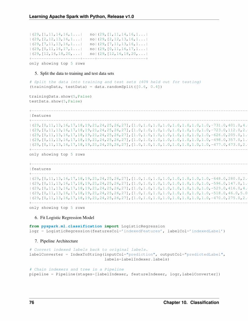
Learning Apache Spark with Python, Release v1.0
|(29,[1,11,14,16,1...| no|(29,[1,11,14,16,1...||(29,[2,12,13,16,1...| no|(29,[2,12,13,16,1...||(29,[7,11,13,16,1...| no|(29,[7,11,13,16,1...||(29,[0,11,16,17,1...| no|(29,[0,11,16,17,1...||(29,[12,16,18,20,...| no|(29,[12,16,18,20,...|+--------------------+-----+--------------------+only showing top 5 rows
5. Split the data to training and test data sets
# Split the data into training and test sets (40% held out for testing)(trainingData, testData) = data.randomSplit([0.6, 0.4])
trainingData.show(5,False)testData.show(5,False)
+-------------------------------------------------------------------------------------------------+-----+|features |label|+-------------------------------------------------------------------------------------------------+-----+|(29,[0,11,13,16,17,18,19,21,24,25,26,27],[1.0,1.0,1.0,1.0,1.0,1.0,1.0,1.0,-731.0,401.0,4.0,-1.0])|no ||(29,[0,11,13,16,17,18,19,21,24,25,26,27],[1.0,1.0,1.0,1.0,1.0,1.0,1.0,1.0,-723.0,112.0,2.0,-1.0])|no ||(29,[0,11,13,16,17,18,19,21,24,25,26,27],[1.0,1.0,1.0,1.0,1.0,1.0,1.0,1.0,-626.0,205.0,1.0,-1.0])|no ||(29,[0,11,13,16,17,18,19,21,24,25,26,27],[1.0,1.0,1.0,1.0,1.0,1.0,1.0,1.0,-498.0,357.0,1.0,-1.0])|no ||(29,[0,11,13,16,17,18,19,21,24,25,26,27],[1.0,1.0,1.0,1.0,1.0,1.0,1.0,1.0,-477.0,473.0,2.0,-1.0])|no |+-------------------------------------------------------------------------------------------------+-----+only showing top 5 rows
+-------------------------------------------------------------------------------------------------+-----+|features |label|+-------------------------------------------------------------------------------------------------+-----+|(29,[0,11,13,16,17,18,19,21,24,25,26,27],[1.0,1.0,1.0,1.0,1.0,1.0,1.0,1.0,-648.0,280.0,2.0,-1.0])|no ||(29,[0,11,13,16,17,18,19,21,24,25,26,27],[1.0,1.0,1.0,1.0,1.0,1.0,1.0,1.0,-596.0,147.0,1.0,-1.0])|no ||(29,[0,11,13,16,17,18,19,21,24,25,26,27],[1.0,1.0,1.0,1.0,1.0,1.0,1.0,1.0,-529.0,416.0,4.0,-1.0])|no ||(29,[0,11,13,16,17,18,19,21,24,25,26,27],[1.0,1.0,1.0,1.0,1.0,1.0,1.0,1.0,-518.0,46.0,5.0,-1.0]) |no ||(29,[0,11,13,16,17,18,19,21,24,25,26,27],[1.0,1.0,1.0,1.0,1.0,1.0,1.0,1.0,-470.0,275.0,2.0,-1.0])|no |+-------------------------------------------------------------------------------------------------+-----+only showing top 5 rows
6. Fit Logistic Regression Model
from pyspark.ml.classification import LogisticRegressionlogr = LogisticRegression(featuresCol=’indexedFeatures’, labelCol=’indexedLabel’)
7. Pipeline Architecture
# Convert indexed labels back to original labels.labelConverter = IndexToString(inputCol="prediction", outputCol="predictedLabel",
labels=labelIndexer.labels)
# Chain indexers and tree in a Pipelinepipeline = Pipeline(stages=[labelIndexer, featureIndexer, logr,labelConverter])
76 Chapter 10. Classification
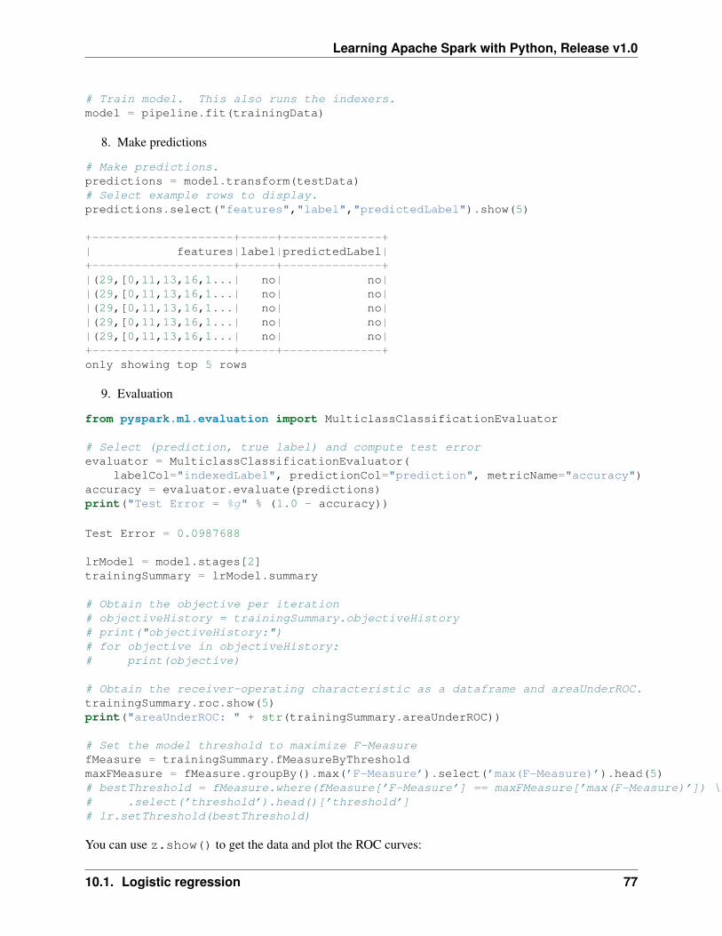
Learning Apache Spark with Python, Release v1.0
# Train model. This also runs the indexers.model = pipeline.fit(trainingData)
8. Make predictions
# Make predictions.predictions = model.transform(testData)# Select example rows to display.predictions.select("features","label","predictedLabel").show(5)
+--------------------+-----+--------------+| features|label|predictedLabel|+--------------------+-----+--------------+|(29,[0,11,13,16,1...| no| no||(29,[0,11,13,16,1...| no| no||(29,[0,11,13,16,1...| no| no||(29,[0,11,13,16,1...| no| no||(29,[0,11,13,16,1...| no| no|+--------------------+-----+--------------+only showing top 5 rows
9. Evaluation
from pyspark.ml.evaluation import MulticlassClassificationEvaluator
# Select (prediction, true label) and compute test errorevaluator = MulticlassClassificationEvaluator(
labelCol="indexedLabel", predictionCol="prediction", metricName="accuracy")accuracy = evaluator.evaluate(predictions)print("Test Error = %g" % (1.0 - accuracy))
Test Error = 0.0987688
lrModel = model.stages[2]trainingSummary = lrModel.summary
# Obtain the objective per iteration# objectiveHistory = trainingSummary.objectiveHistory# print("objectiveHistory:")# for objective in objectiveHistory:# print(objective)
# Obtain the receiver-operating characteristic as a dataframe and areaUnderROC.trainingSummary.roc.show(5)print("areaUnderROC: " + str(trainingSummary.areaUnderROC))
# Set the model threshold to maximize F-MeasurefMeasure = trainingSummary.fMeasureByThresholdmaxFMeasure = fMeasure.groupBy().max(’F-Measure’).select(’max(F-Measure)’).head(5)# bestThreshold = fMeasure.where(fMeasure[’F-Measure’] == maxFMeasure[’max(F-Measure)’]) \# .select(’threshold’).head()[’threshold’]# lr.setThreshold(bestThreshold)
You can use z.show() to get the data and plot the ROC curves:
10.1. Logistic regression 77
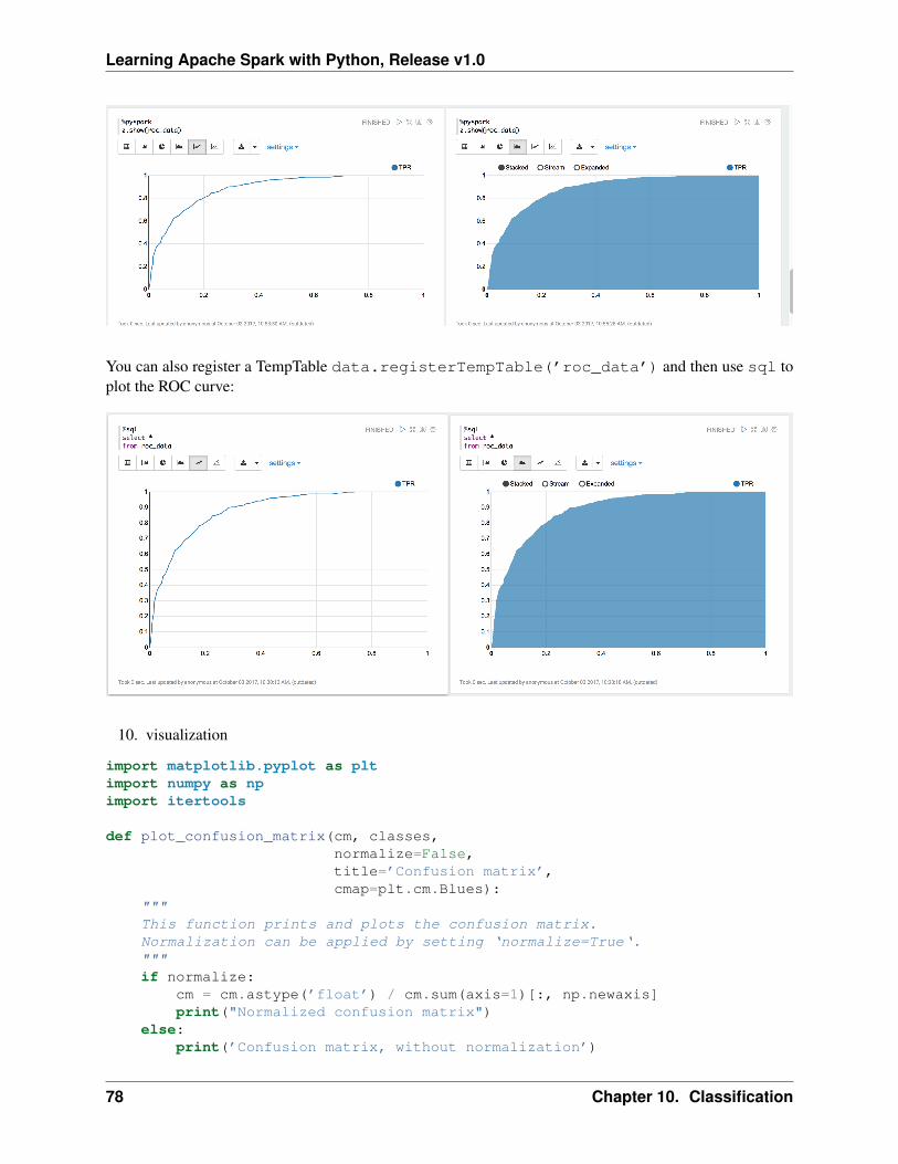
Learning Apache Spark with Python, Release v1.0
You can also register a TempTable data.registerTempTable(’roc_data’) and then use sql toplot the ROC curve:
10. visualization
import matplotlib.pyplot as pltimport numpy as npimport itertools
def plot_confusion_matrix(cm, classes,normalize=False,title=’Confusion matrix’,cmap=plt.cm.Blues):
"""This function prints and plots the confusion matrix.Normalization can be applied by setting ‘normalize=True‘."""if normalize:
cm = cm.astype(’float’) / cm.sum(axis=1)[:, np.newaxis]print("Normalized confusion matrix")
else:print(’Confusion matrix, without normalization’)
78 Chapter 10. Classification
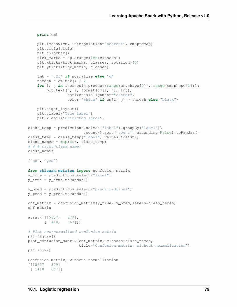
Learning Apache Spark with Python, Release v1.0
print(cm)
plt.imshow(cm, interpolation=’nearest’, cmap=cmap)plt.title(title)plt.colorbar()tick_marks = np.arange(len(classes))plt.xticks(tick_marks, classes, rotation=45)plt.yticks(tick_marks, classes)
fmt = ’.2f’ if normalize else ’d’thresh = cm.max() / 2.for i, j in itertools.product(range(cm.shape[0]), range(cm.shape[1])):
plt.text(j, i, format(cm[i, j], fmt),horizontalalignment="center",color="white" if cm[i, j] > thresh else "black")
plt.tight_layout()plt.ylabel(’True label’)plt.xlabel(’Predicted label’)
class_temp = predictions.select("label").groupBy("label")\.count().sort(’count’, ascending=False).toPandas()
class_temp = class_temp["label"].values.tolist()class_names = map(str, class_temp)# # # print(class_name)class_names
[’no’, ’yes’]
from sklearn.metrics import confusion_matrixy_true = predictions.select("label")y_true = y_true.toPandas()
y_pred = predictions.select("predictedLabel")y_pred = y_pred.toPandas()
cnf_matrix = confusion_matrix(y_true, y_pred,labels=class_names)cnf_matrix
array([[15657, 379],[ 1410, 667]])
# Plot non-normalized confusion matrixplt.figure()plot_confusion_matrix(cnf_matrix, classes=class_names,
title=’Confusion matrix, without normalization’)plt.show()
Confusion matrix, without normalization[[15657 379][ 1410 667]]
10.1. Logistic regression 79
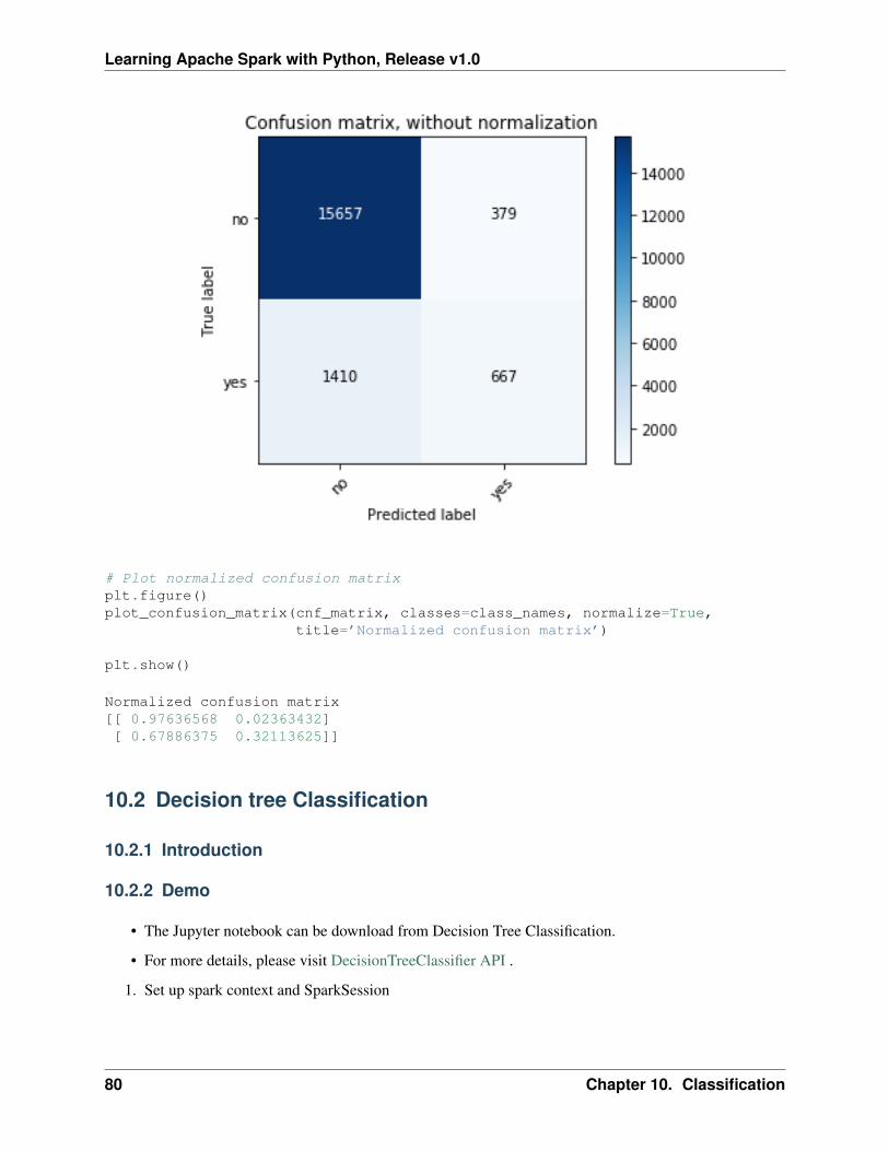
Learning Apache Spark with Python, Release v1.0
# Plot normalized confusion matrixplt.figure()plot_confusion_matrix(cnf_matrix, classes=class_names, normalize=True,
title=’Normalized confusion matrix’)
plt.show()
Normalized confusion matrix[[ 0.97636568 0.02363432][ 0.67886375 0.32113625]]
10.2 Decision tree Classification
10.2.1 Introduction
10.2.2 Demo
• The Jupyter notebook can be download from Decision Tree Classification.
• For more details, please visit DecisionTreeClassifier API .
1. Set up spark context and SparkSession
80 Chapter 10. Classification
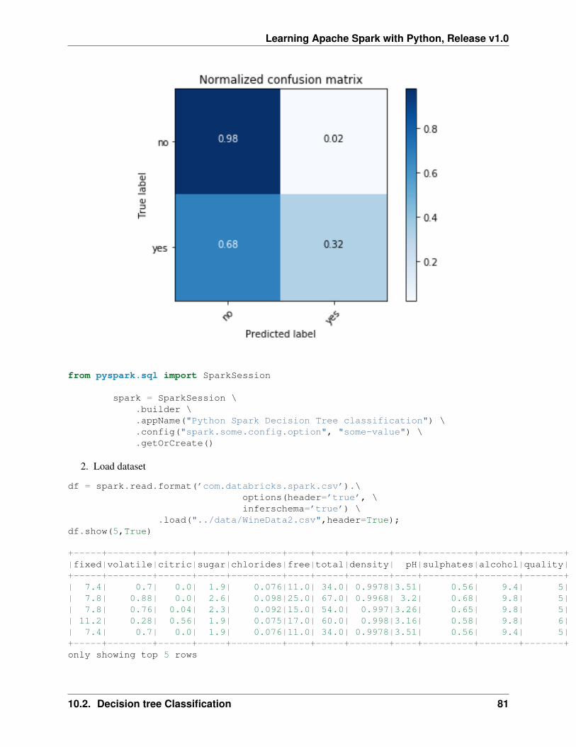
Learning Apache Spark with Python, Release v1.0
from pyspark.sql import SparkSession
spark = SparkSession \.builder \.appName("Python Spark Decision Tree classification") \.config("spark.some.config.option", "some-value") \.getOrCreate()
2. Load dataset
df = spark.read.format(’com.databricks.spark.csv’).\options(header=’true’, \inferschema=’true’) \
.load("../data/WineData2.csv",header=True);df.show(5,True)
+-----+--------+------+-----+---------+----+-----+-------+----+---------+-------+-------+|fixed|volatile|citric|sugar|chlorides|free|total|density| pH|sulphates|alcohol|quality|+-----+--------+------+-----+---------+----+-----+-------+----+---------+-------+-------+| 7.4| 0.7| 0.0| 1.9| 0.076|11.0| 34.0| 0.9978|3.51| 0.56| 9.4| 5|| 7.8| 0.88| 0.0| 2.6| 0.098|25.0| 67.0| 0.9968| 3.2| 0.68| 9.8| 5|| 7.8| 0.76| 0.04| 2.3| 0.092|15.0| 54.0| 0.997|3.26| 0.65| 9.8| 5|| 11.2| 0.28| 0.56| 1.9| 0.075|17.0| 60.0| 0.998|3.16| 0.58| 9.8| 6|| 7.4| 0.7| 0.0| 1.9| 0.076|11.0| 34.0| 0.9978|3.51| 0.56| 9.4| 5|+-----+--------+------+-----+---------+----+-----+-------+----+---------+-------+-------+only showing top 5 rows
10.2. Decision tree Classification 81
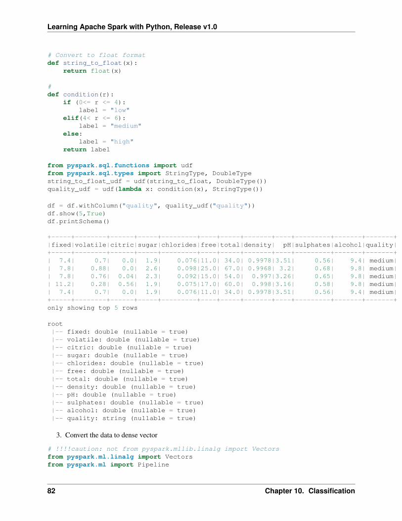
Learning Apache Spark with Python, Release v1.0
# Convert to float formatdef string_to_float(x):
return float(x)
#def condition(r):
if (0<= r <= 4):label = "low"
elif(4< r <= 6):label = "medium"
else:label = "high"
return label
from pyspark.sql.functions import udffrom pyspark.sql.types import StringType, DoubleTypestring_to_float_udf = udf(string_to_float, DoubleType())quality_udf = udf(lambda x: condition(x), StringType())
df = df.withColumn("quality", quality_udf("quality"))df.show(5,True)df.printSchema()
+-----+--------+------+-----+---------+----+-----+-------+----+---------+-------+-------+|fixed|volatile|citric|sugar|chlorides|free|total|density| pH|sulphates|alcohol|quality|+-----+--------+------+-----+---------+----+-----+-------+----+---------+-------+-------+| 7.4| 0.7| 0.0| 1.9| 0.076|11.0| 34.0| 0.9978|3.51| 0.56| 9.4| medium|| 7.8| 0.88| 0.0| 2.6| 0.098|25.0| 67.0| 0.9968| 3.2| 0.68| 9.8| medium|| 7.8| 0.76| 0.04| 2.3| 0.092|15.0| 54.0| 0.997|3.26| 0.65| 9.8| medium|| 11.2| 0.28| 0.56| 1.9| 0.075|17.0| 60.0| 0.998|3.16| 0.58| 9.8| medium|| 7.4| 0.7| 0.0| 1.9| 0.076|11.0| 34.0| 0.9978|3.51| 0.56| 9.4| medium|+-----+--------+------+-----+---------+----+-----+-------+----+---------+-------+-------+only showing top 5 rows
root|-- fixed: double (nullable = true)|-- volatile: double (nullable = true)|-- citric: double (nullable = true)|-- sugar: double (nullable = true)|-- chlorides: double (nullable = true)|-- free: double (nullable = true)|-- total: double (nullable = true)|-- density: double (nullable = true)|-- pH: double (nullable = true)|-- sulphates: double (nullable = true)|-- alcohol: double (nullable = true)|-- quality: string (nullable = true)
3. Convert the data to dense vector
# !!!!caution: not from pyspark.mllib.linalg import Vectorsfrom pyspark.ml.linalg import Vectorsfrom pyspark.ml import Pipeline
82 Chapter 10. Classification
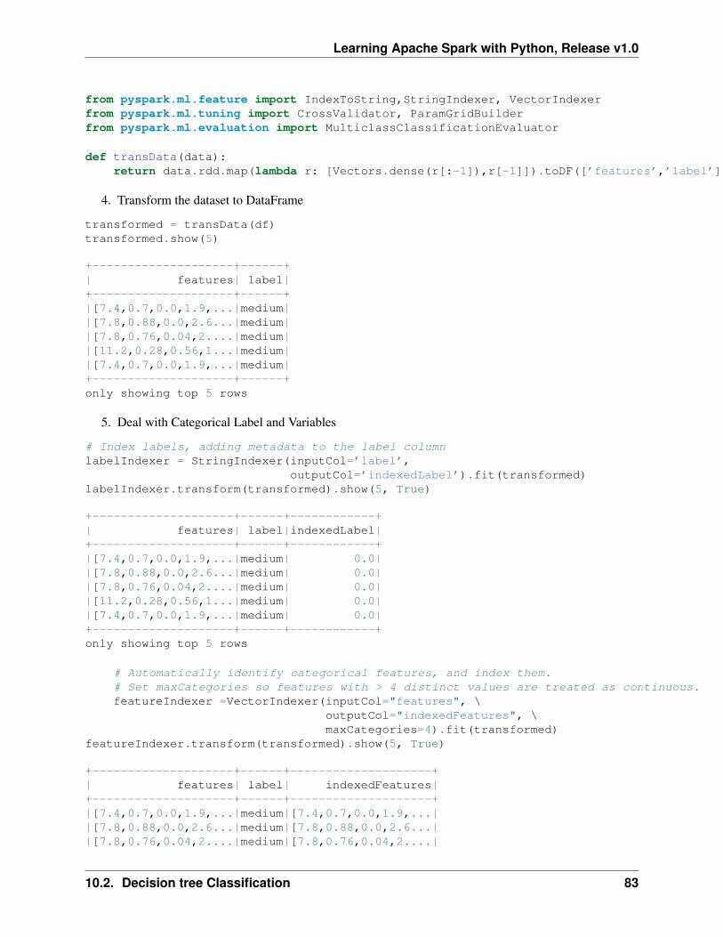
Learning Apache Spark with Python, Release v1.0
from pyspark.ml.feature import IndexToString,StringIndexer, VectorIndexerfrom pyspark.ml.tuning import CrossValidator, ParamGridBuilderfrom pyspark.ml.evaluation import MulticlassClassificationEvaluator
def transData(data):return data.rdd.map(lambda r: [Vectors.dense(r[:-1]),r[-1]]).toDF([’features’,’label’])
4. Transform the dataset to DataFrame
transformed = transData(df)transformed.show(5)
+--------------------+------+| features| label|+--------------------+------+|[7.4,0.7,0.0,1.9,...|medium||[7.8,0.88,0.0,2.6...|medium||[7.8,0.76,0.04,2....|medium||[11.2,0.28,0.56,1...|medium||[7.4,0.7,0.0,1.9,...|medium|+--------------------+------+only showing top 5 rows
5. Deal with Categorical Label and Variables
# Index labels, adding metadata to the label columnlabelIndexer = StringIndexer(inputCol=’label’,
outputCol=’indexedLabel’).fit(transformed)labelIndexer.transform(transformed).show(5, True)
+--------------------+------+------------+| features| label|indexedLabel|+--------------------+------+------------+|[7.4,0.7,0.0,1.9,...|medium| 0.0||[7.8,0.88,0.0,2.6...|medium| 0.0||[7.8,0.76,0.04,2....|medium| 0.0||[11.2,0.28,0.56,1...|medium| 0.0||[7.4,0.7,0.0,1.9,...|medium| 0.0|+--------------------+------+------------+only showing top 5 rows
# Automatically identify categorical features, and index them.# Set maxCategories so features with > 4 distinct values are treated as continuous.featureIndexer =VectorIndexer(inputCol="features", \
outputCol="indexedFeatures", \maxCategories=4).fit(transformed)
featureIndexer.transform(transformed).show(5, True)
+--------------------+------+--------------------+| features| label| indexedFeatures|+--------------------+------+--------------------+|[7.4,0.7,0.0,1.9,...|medium|[7.4,0.7,0.0,1.9,...||[7.8,0.88,0.0,2.6...|medium|[7.8,0.88,0.0,2.6...||[7.8,0.76,0.04,2....|medium|[7.8,0.76,0.04,2....|
10.2. Decision tree Classification 83
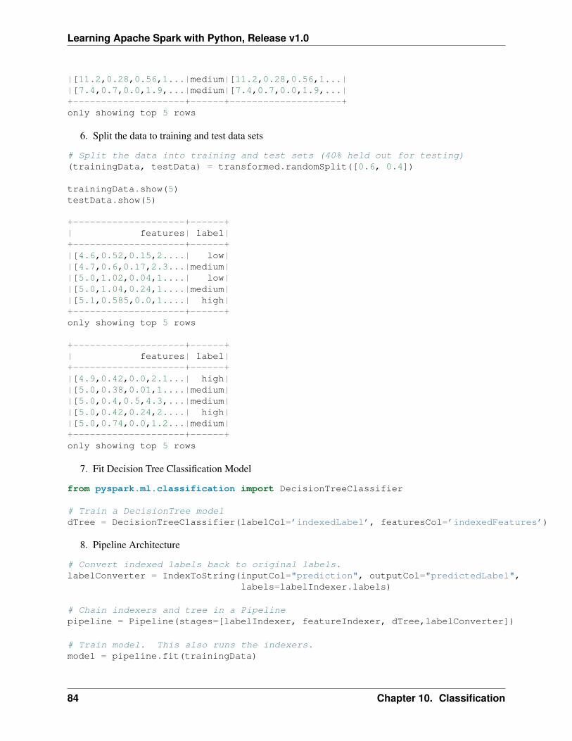
Learning Apache Spark with Python, Release v1.0
|[11.2,0.28,0.56,1...|medium|[11.2,0.28,0.56,1...||[7.4,0.7,0.0,1.9,...|medium|[7.4,0.7,0.0,1.9,...|+--------------------+------+--------------------+only showing top 5 rows
6. Split the data to training and test data sets
# Split the data into training and test sets (40% held out for testing)(trainingData, testData) = transformed.randomSplit([0.6, 0.4])
trainingData.show(5)testData.show(5)
+--------------------+------+| features| label|+--------------------+------+|[4.6,0.52,0.15,2....| low||[4.7,0.6,0.17,2.3...|medium||[5.0,1.02,0.04,1....| low||[5.0,1.04,0.24,1....|medium||[5.1,0.585,0.0,1....| high|+--------------------+------+only showing top 5 rows
+--------------------+------+| features| label|+--------------------+------+|[4.9,0.42,0.0,2.1...| high||[5.0,0.38,0.01,1....|medium||[5.0,0.4,0.5,4.3,...|medium||[5.0,0.42,0.24,2....| high||[5.0,0.74,0.0,1.2...|medium|+--------------------+------+only showing top 5 rows
7. Fit Decision Tree Classification Model
from pyspark.ml.classification import DecisionTreeClassifier
# Train a DecisionTree modeldTree = DecisionTreeClassifier(labelCol=’indexedLabel’, featuresCol=’indexedFeatures’)
8. Pipeline Architecture
# Convert indexed labels back to original labels.labelConverter = IndexToString(inputCol="prediction", outputCol="predictedLabel",
labels=labelIndexer.labels)
# Chain indexers and tree in a Pipelinepipeline = Pipeline(stages=[labelIndexer, featureIndexer, dTree,labelConverter])
# Train model. This also runs the indexers.model = pipeline.fit(trainingData)
84 Chapter 10. Classification
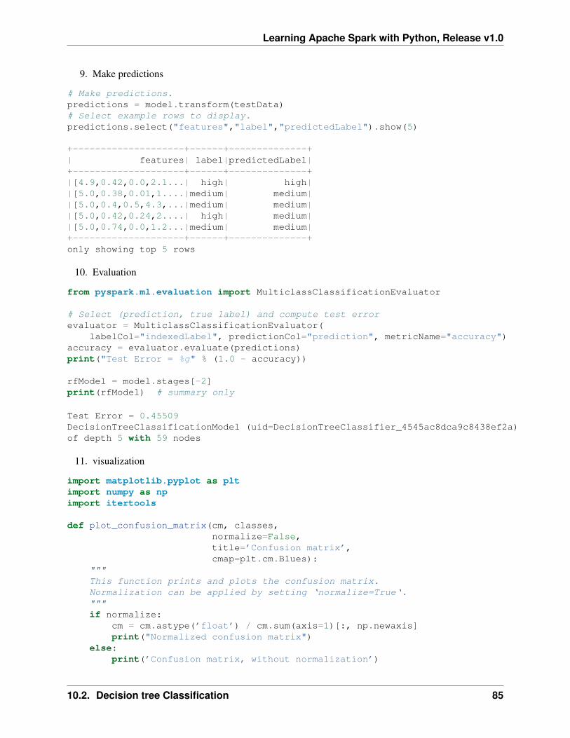
Learning Apache Spark with Python, Release v1.0
9. Make predictions
# Make predictions.predictions = model.transform(testData)# Select example rows to display.predictions.select("features","label","predictedLabel").show(5)
+--------------------+------+--------------+| features| label|predictedLabel|+--------------------+------+--------------+|[4.9,0.42,0.0,2.1...| high| high||[5.0,0.38,0.01,1....|medium| medium||[5.0,0.4,0.5,4.3,...|medium| medium||[5.0,0.42,0.24,2....| high| medium||[5.0,0.74,0.0,1.2...|medium| medium|+--------------------+------+--------------+only showing top 5 rows
10. Evaluation
from pyspark.ml.evaluation import MulticlassClassificationEvaluator
# Select (prediction, true label) and compute test errorevaluator = MulticlassClassificationEvaluator(
labelCol="indexedLabel", predictionCol="prediction", metricName="accuracy")accuracy = evaluator.evaluate(predictions)print("Test Error = %g" % (1.0 - accuracy))
rfModel = model.stages[-2]print(rfModel) # summary only
Test Error = 0.45509DecisionTreeClassificationModel (uid=DecisionTreeClassifier_4545ac8dca9c8438ef2a)of depth 5 with 59 nodes
11. visualization
import matplotlib.pyplot as pltimport numpy as npimport itertools
def plot_confusion_matrix(cm, classes,normalize=False,title=’Confusion matrix’,cmap=plt.cm.Blues):
"""This function prints and plots the confusion matrix.Normalization can be applied by setting ‘normalize=True‘."""if normalize:
cm = cm.astype(’float’) / cm.sum(axis=1)[:, np.newaxis]print("Normalized confusion matrix")
else:print(’Confusion matrix, without normalization’)
10.2. Decision tree Classification 85
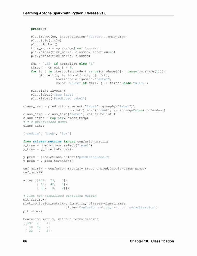
Learning Apache Spark with Python, Release v1.0
print(cm)
plt.imshow(cm, interpolation=’nearest’, cmap=cmap)plt.title(title)plt.colorbar()tick_marks = np.arange(len(classes))plt.xticks(tick_marks, classes, rotation=45)plt.yticks(tick_marks, classes)
fmt = ’.2f’ if normalize else ’d’thresh = cm.max() / 2.for i, j in itertools.product(range(cm.shape[0]), range(cm.shape[1])):
plt.text(j, i, format(cm[i, j], fmt),horizontalalignment="center",color="white" if cm[i, j] > thresh else "black")
plt.tight_layout()plt.ylabel(’True label’)plt.xlabel(’Predicted label’)
class_temp = predictions.select("label").groupBy("label")\.count().sort(’count’, ascending=False).toPandas()
class_temp = class_temp["label"].values.tolist()class_names = map(str, class_temp)# # # print(class_name)class_names
[’medium’, ’high’, ’low’]
from sklearn.metrics import confusion_matrixy_true = predictions.select("label")y_true = y_true.toPandas()
y_pred = predictions.select("predictedLabel")y_pred = y_pred.toPandas()
cnf_matrix = confusion_matrix(y_true, y_pred,labels=class_names)cnf_matrix
array([[497, 29, 7],[ 40, 42, 0],[ 22, 0, 2]])
# Plot non-normalized confusion matrixplt.figure()plot_confusion_matrix(cnf_matrix, classes=class_names,
title=’Confusion matrix, without normalization’)plt.show()
Confusion matrix, without normalization[[497 29 7][ 40 42 0][ 22 0 2]]
86 Chapter 10. Classification
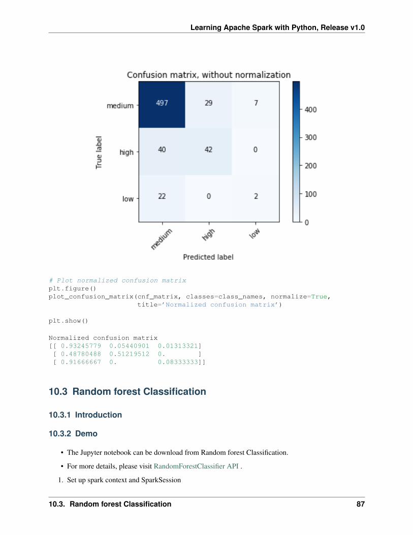
Learning Apache Spark with Python, Release v1.0
# Plot normalized confusion matrixplt.figure()plot_confusion_matrix(cnf_matrix, classes=class_names, normalize=True,
title=’Normalized confusion matrix’)
plt.show()
Normalized confusion matrix[[ 0.93245779 0.05440901 0.01313321][ 0.48780488 0.51219512 0. ][ 0.91666667 0. 0.08333333]]
10.3 Random forest Classification
10.3.1 Introduction
10.3.2 Demo
• The Jupyter notebook can be download from Random forest Classification.
• For more details, please visit RandomForestClassifier API .
1. Set up spark context and SparkSession
10.3. Random forest Classification 87
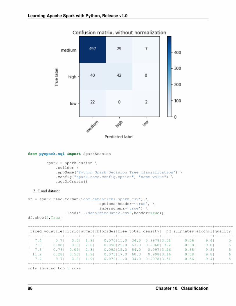
Learning Apache Spark with Python, Release v1.0
from pyspark.sql import SparkSession
spark = SparkSession \.builder \.appName("Python Spark Decision Tree classification") \.config("spark.some.config.option", "some-value") \.getOrCreate()
2. Load dataset
df = spark.read.format(’com.databricks.spark.csv’).\options(header=’true’, \inferschema=’true’) \
.load("../data/WineData2.csv",header=True);df.show(5,True)
+-----+--------+------+-----+---------+----+-----+-------+----+---------+-------+-------+|fixed|volatile|citric|sugar|chlorides|free|total|density| pH|sulphates|alcohol|quality|+-----+--------+------+-----+---------+----+-----+-------+----+---------+-------+-------+| 7.4| 0.7| 0.0| 1.9| 0.076|11.0| 34.0| 0.9978|3.51| 0.56| 9.4| 5|| 7.8| 0.88| 0.0| 2.6| 0.098|25.0| 67.0| 0.9968| 3.2| 0.68| 9.8| 5|| 7.8| 0.76| 0.04| 2.3| 0.092|15.0| 54.0| 0.997|3.26| 0.65| 9.8| 5|| 11.2| 0.28| 0.56| 1.9| 0.075|17.0| 60.0| 0.998|3.16| 0.58| 9.8| 6|| 7.4| 0.7| 0.0| 1.9| 0.076|11.0| 34.0| 0.9978|3.51| 0.56| 9.4| 5|+-----+--------+------+-----+---------+----+-----+-------+----+---------+-------+-------+only showing top 5 rows
88 Chapter 10. Classification

Learning Apache Spark with Python, Release v1.0
# Convert to float formatdef string_to_float(x):
return float(x)
#def condition(r):
if (0<= r <= 4):label = "low"
elif(4< r <= 6):label = "medium"
else:label = "high"
return label
from pyspark.sql.functions import udffrom pyspark.sql.types import StringType, DoubleTypestring_to_float_udf = udf(string_to_float, DoubleType())quality_udf = udf(lambda x: condition(x), StringType())
df = df.withColumn("quality", quality_udf("quality"))df.show(5,True)df.printSchema()
+-----+--------+------+-----+---------+----+-----+-------+----+---------+-------+-------+|fixed|volatile|citric|sugar|chlorides|free|total|density| pH|sulphates|alcohol|quality|+-----+--------+------+-----+---------+----+-----+-------+----+---------+-------+-------+| 7.4| 0.7| 0.0| 1.9| 0.076|11.0| 34.0| 0.9978|3.51| 0.56| 9.4| medium|| 7.8| 0.88| 0.0| 2.6| 0.098|25.0| 67.0| 0.9968| 3.2| 0.68| 9.8| medium|| 7.8| 0.76| 0.04| 2.3| 0.092|15.0| 54.0| 0.997|3.26| 0.65| 9.8| medium|| 11.2| 0.28| 0.56| 1.9| 0.075|17.0| 60.0| 0.998|3.16| 0.58| 9.8| medium|| 7.4| 0.7| 0.0| 1.9| 0.076|11.0| 34.0| 0.9978|3.51| 0.56| 9.4| medium|+-----+--------+------+-----+---------+----+-----+-------+----+---------+-------+-------+only showing top 5 rows
root|-- fixed: double (nullable = true)|-- volatile: double (nullable = true)|-- citric: double (nullable = true)|-- sugar: double (nullable = true)|-- chlorides: double (nullable = true)|-- free: double (nullable = true)|-- total: double (nullable = true)|-- density: double (nullable = true)|-- pH: double (nullable = true)|-- sulphates: double (nullable = true)|-- alcohol: double (nullable = true)|-- quality: string (nullable = true)
3. Convert the data to dense vector
# !!!!caution: not from pyspark.mllib.linalg import Vectorsfrom pyspark.ml.linalg import Vectorsfrom pyspark.ml import Pipeline
10.3. Random forest Classification 89
Learning Apache Spark with Python, Release v1.0
from pyspark.ml.feature import IndexToString,StringIndexer, VectorIndexerfrom pyspark.ml.tuning import CrossValidator, ParamGridBuilderfrom pyspark.ml.evaluation import MulticlassClassificationEvaluator
def transData(data):return data.rdd.map(lambda r: [Vectors.dense(r[:-1]),r[-1]]).toDF([’features’,’label’])
4. Transform the dataset to DataFrame
transformed = transData(df)transformed.show(5)
+--------------------+------+| features| label|+--------------------+------+|[7.4,0.7,0.0,1.9,...|medium||[7.8,0.88,0.0,2.6...|medium||[7.8,0.76,0.04,2....|medium||[11.2,0.28,0.56,1...|medium||[7.4,0.7,0.0,1.9,...|medium|+--------------------+------+only showing top 5 rows
5. Deal with Categorical Label and Variables
# Index labels, adding metadata to the label columnlabelIndexer = StringIndexer(inputCol=’label’,
outputCol=’indexedLabel’).fit(transformed)labelIndexer.transform(transformed).show(5, True)
+--------------------+------+------------+| features| label|indexedLabel|+--------------------+------+------------+|[7.4,0.7,0.0,1.9,...|medium| 0.0||[7.8,0.88,0.0,2.6...|medium| 0.0||[7.8,0.76,0.04,2....|medium| 0.0||[11.2,0.28,0.56,1...|medium| 0.0||[7.4,0.7,0.0,1.9,...|medium| 0.0|+--------------------+------+------------+only showing top 5 rows
# Automatically identify categorical features, and index them.# Set maxCategories so features with > 4 distinct values are treated as continuous.featureIndexer =VectorIndexer(inputCol="features", \
outputCol="indexedFeatures", \maxCategories=4).fit(transformed)
featureIndexer.transform(transformed).show(5, True)
+--------------------+------+--------------------+| features| label| indexedFeatures|+--------------------+------+--------------------+|[7.4,0.7,0.0,1.9,...|medium|[7.4,0.7,0.0,1.9,...||[7.8,0.88,0.0,2.6...|medium|[7.8,0.88,0.0,2.6...||[7.8,0.76,0.04,2....|medium|[7.8,0.76,0.04,2....|
90 Chapter 10. Classification
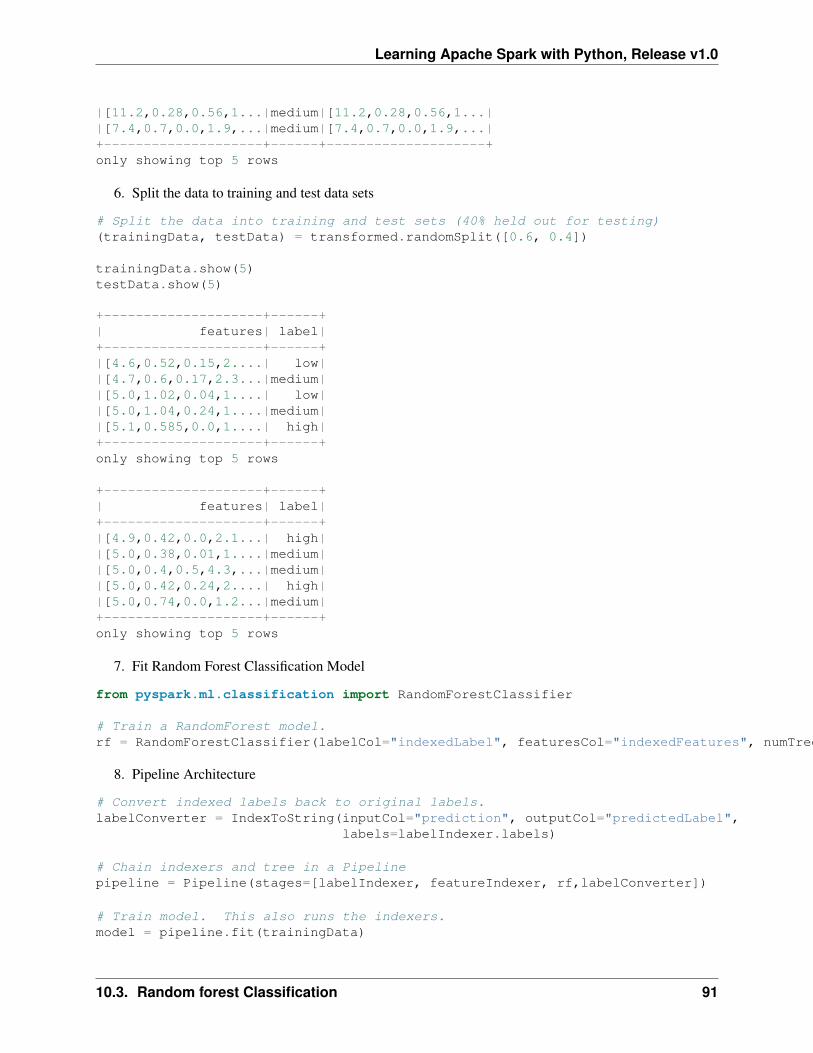
Learning Apache Spark with Python, Release v1.0
|[11.2,0.28,0.56,1...|medium|[11.2,0.28,0.56,1...||[7.4,0.7,0.0,1.9,...|medium|[7.4,0.7,0.0,1.9,...|+--------------------+------+--------------------+only showing top 5 rows
6. Split the data to training and test data sets
# Split the data into training and test sets (40% held out for testing)(trainingData, testData) = transformed.randomSplit([0.6, 0.4])
trainingData.show(5)testData.show(5)
+--------------------+------+| features| label|+--------------------+------+|[4.6,0.52,0.15,2....| low||[4.7,0.6,0.17,2.3...|medium||[5.0,1.02,0.04,1....| low||[5.0,1.04,0.24,1....|medium||[5.1,0.585,0.0,1....| high|+--------------------+------+only showing top 5 rows
+--------------------+------+| features| label|+--------------------+------+|[4.9,0.42,0.0,2.1...| high||[5.0,0.38,0.01,1....|medium||[5.0,0.4,0.5,4.3,...|medium||[5.0,0.42,0.24,2....| high||[5.0,0.74,0.0,1.2...|medium|+--------------------+------+only showing top 5 rows
7. Fit Random Forest Classification Model
from pyspark.ml.classification import RandomForestClassifier
# Train a RandomForest model.rf = RandomForestClassifier(labelCol="indexedLabel", featuresCol="indexedFeatures", numTrees=10)
8. Pipeline Architecture
# Convert indexed labels back to original labels.labelConverter = IndexToString(inputCol="prediction", outputCol="predictedLabel",
labels=labelIndexer.labels)
# Chain indexers and tree in a Pipelinepipeline = Pipeline(stages=[labelIndexer, featureIndexer, rf,labelConverter])
# Train model. This also runs the indexers.model = pipeline.fit(trainingData)
10.3. Random forest Classification 91
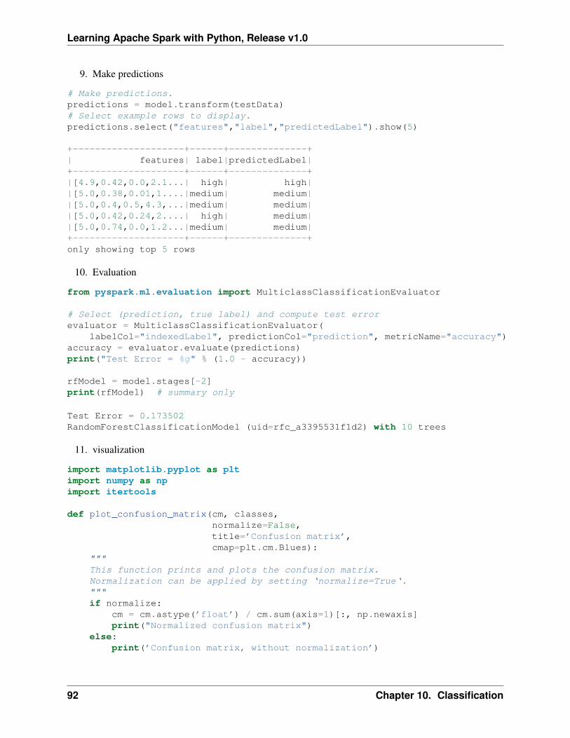
Learning Apache Spark with Python, Release v1.0
9. Make predictions
# Make predictions.predictions = model.transform(testData)# Select example rows to display.predictions.select("features","label","predictedLabel").show(5)
+--------------------+------+--------------+| features| label|predictedLabel|+--------------------+------+--------------+|[4.9,0.42,0.0,2.1...| high| high||[5.0,0.38,0.01,1....|medium| medium||[5.0,0.4,0.5,4.3,...|medium| medium||[5.0,0.42,0.24,2....| high| medium||[5.0,0.74,0.0,1.2...|medium| medium|+--------------------+------+--------------+only showing top 5 rows
10. Evaluation
from pyspark.ml.evaluation import MulticlassClassificationEvaluator
# Select (prediction, true label) and compute test errorevaluator = MulticlassClassificationEvaluator(
labelCol="indexedLabel", predictionCol="prediction", metricName="accuracy")accuracy = evaluator.evaluate(predictions)print("Test Error = %g" % (1.0 - accuracy))
rfModel = model.stages[-2]print(rfModel) # summary only
Test Error = 0.173502RandomForestClassificationModel (uid=rfc_a3395531f1d2) with 10 trees
11. visualization
import matplotlib.pyplot as pltimport numpy as npimport itertools
def plot_confusion_matrix(cm, classes,normalize=False,title=’Confusion matrix’,cmap=plt.cm.Blues):
"""This function prints and plots the confusion matrix.Normalization can be applied by setting ‘normalize=True‘."""if normalize:
cm = cm.astype(’float’) / cm.sum(axis=1)[:, np.newaxis]print("Normalized confusion matrix")
else:print(’Confusion matrix, without normalization’)
92 Chapter 10. Classification
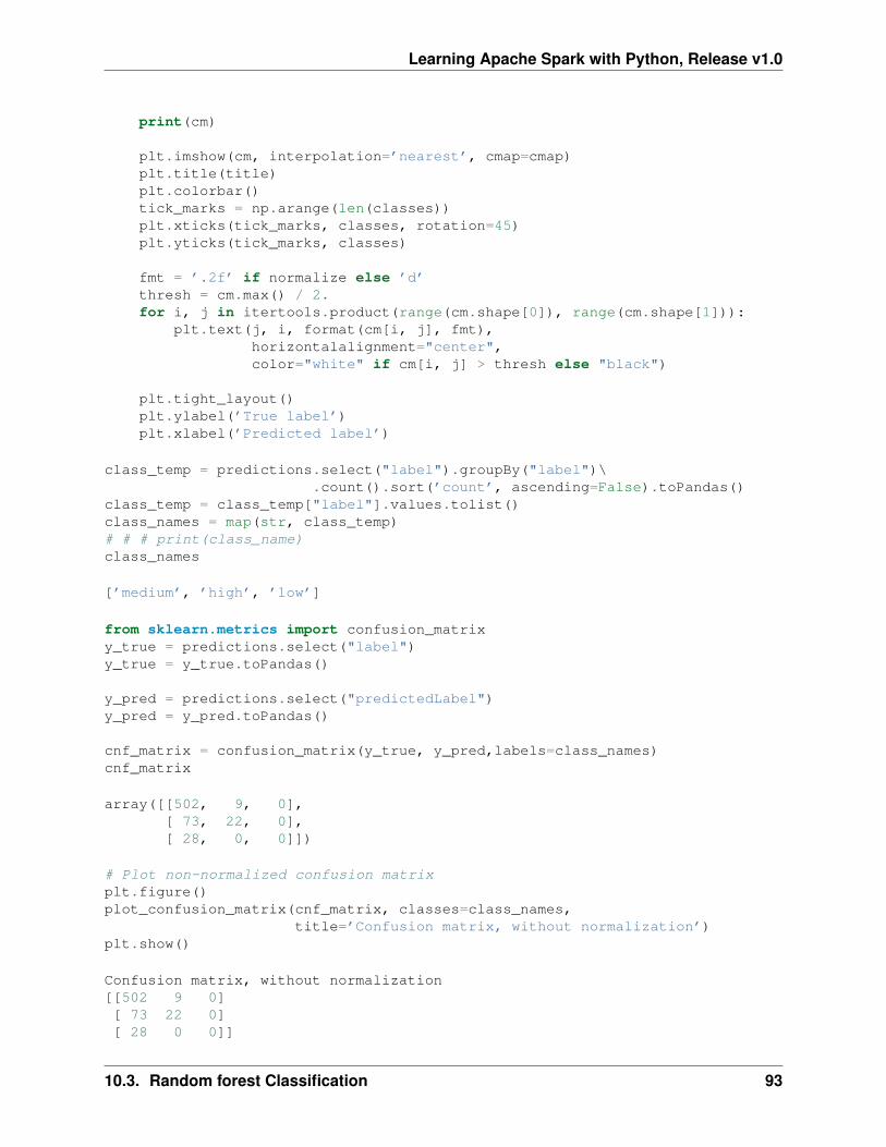
Learning Apache Spark with Python, Release v1.0
print(cm)
plt.imshow(cm, interpolation=’nearest’, cmap=cmap)plt.title(title)plt.colorbar()tick_marks = np.arange(len(classes))plt.xticks(tick_marks, classes, rotation=45)plt.yticks(tick_marks, classes)
fmt = ’.2f’ if normalize else ’d’thresh = cm.max() / 2.for i, j in itertools.product(range(cm.shape[0]), range(cm.shape[1])):
plt.text(j, i, format(cm[i, j], fmt),horizontalalignment="center",color="white" if cm[i, j] > thresh else "black")
plt.tight_layout()plt.ylabel(’True label’)plt.xlabel(’Predicted label’)
class_temp = predictions.select("label").groupBy("label")\.count().sort(’count’, ascending=False).toPandas()
class_temp = class_temp["label"].values.tolist()class_names = map(str, class_temp)# # # print(class_name)class_names
[’medium’, ’high’, ’low’]
from sklearn.metrics import confusion_matrixy_true = predictions.select("label")y_true = y_true.toPandas()
y_pred = predictions.select("predictedLabel")y_pred = y_pred.toPandas()
cnf_matrix = confusion_matrix(y_true, y_pred,labels=class_names)cnf_matrix
array([[502, 9, 0],[ 73, 22, 0],[ 28, 0, 0]])
# Plot non-normalized confusion matrixplt.figure()plot_confusion_matrix(cnf_matrix, classes=class_names,
title=’Confusion matrix, without normalization’)plt.show()
Confusion matrix, without normalization[[502 9 0][ 73 22 0][ 28 0 0]]
10.3. Random forest Classification 93
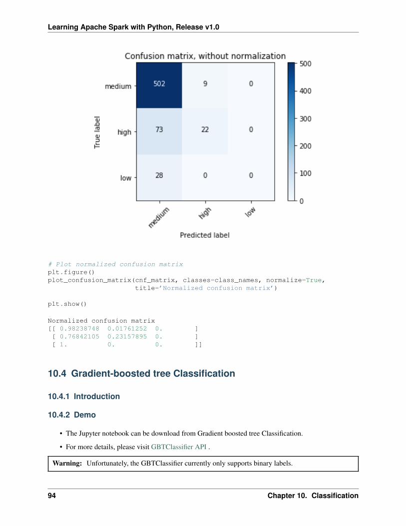
Learning Apache Spark with Python, Release v1.0
# Plot normalized confusion matrixplt.figure()plot_confusion_matrix(cnf_matrix, classes=class_names, normalize=True,
title=’Normalized confusion matrix’)
plt.show()
Normalized confusion matrix[[ 0.98238748 0.01761252 0. ][ 0.76842105 0.23157895 0. ][ 1. 0. 0. ]]
10.4 Gradient-boosted tree Classification
10.4.1 Introduction
10.4.2 Demo
• The Jupyter notebook can be download from Gradient boosted tree Classification.
• For more details, please visit GBTClassifier API .
Warning: Unfortunately, the GBTClassifier currently only supports binary labels.
94 Chapter 10. Classification
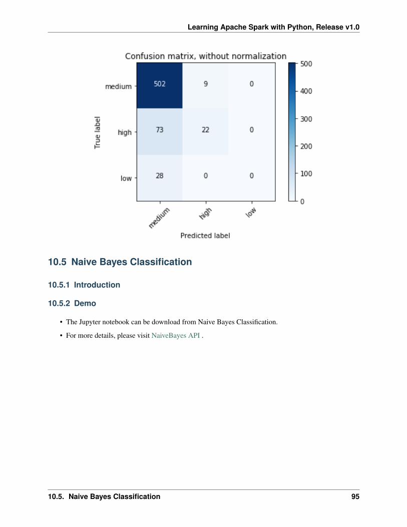
Learning Apache Spark with Python, Release v1.0
10.5 Naive Bayes Classification
10.5.1 Introduction
10.5.2 Demo
• The Jupyter notebook can be download from Naive Bayes Classification.
• For more details, please visit NaiveBayes API .
10.5. Naive Bayes Classification 95

Learning Apache Spark with Python, Release v1.0
96 Chapter 10. Classification
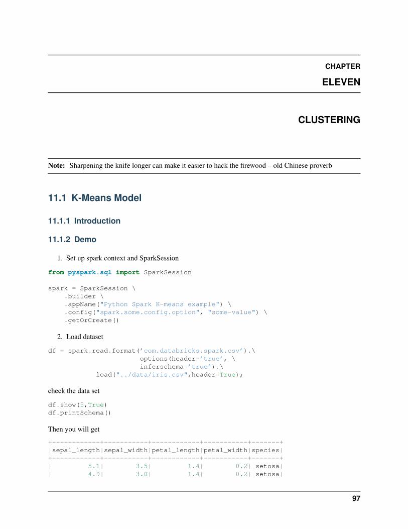
CHAPTER
ELEVEN
CLUSTERING
Note: Sharpening the knife longer can make it easier to hack the firewood – old Chinese proverb
11.1 K-Means Model
11.1.1 Introduction
11.1.2 Demo
1. Set up spark context and SparkSession
from pyspark.sql import SparkSession
spark = SparkSession \.builder \.appName("Python Spark K-means example") \.config("spark.some.config.option", "some-value") \.getOrCreate()
2. Load dataset
df = spark.read.format(’com.databricks.spark.csv’).\options(header=’true’, \inferschema=’true’).\
load("../data/iris.csv",header=True);
check the data set
df.show(5,True)df.printSchema()
Then you will get
+------------+-----------+------------+-----------+-------+|sepal_length|sepal_width|petal_length|petal_width|species|+------------+-----------+------------+-----------+-------+| 5.1| 3.5| 1.4| 0.2| setosa|| 4.9| 3.0| 1.4| 0.2| setosa|
97
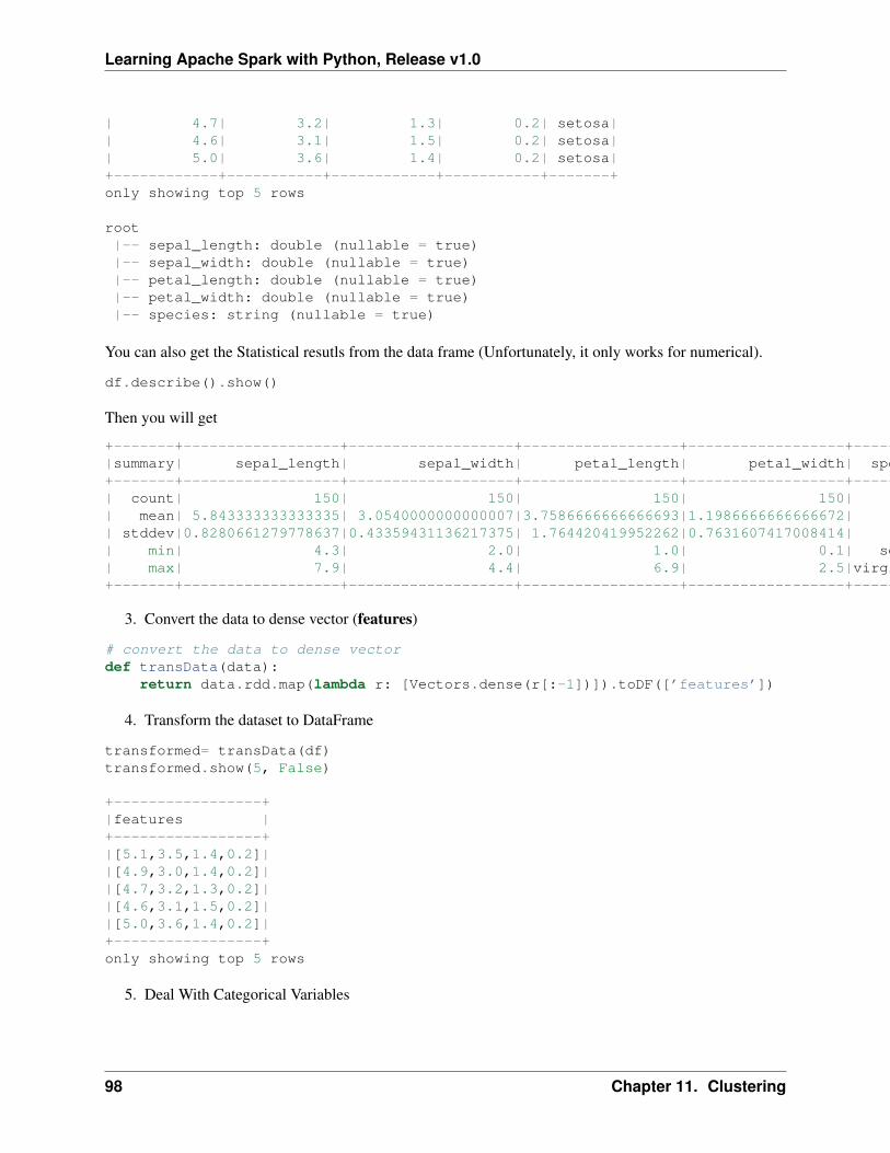
Learning Apache Spark with Python, Release v1.0
| 4.7| 3.2| 1.3| 0.2| setosa|| 4.6| 3.1| 1.5| 0.2| setosa|| 5.0| 3.6| 1.4| 0.2| setosa|+------------+-----------+------------+-----------+-------+only showing top 5 rows
root|-- sepal_length: double (nullable = true)|-- sepal_width: double (nullable = true)|-- petal_length: double (nullable = true)|-- petal_width: double (nullable = true)|-- species: string (nullable = true)
You can also get the Statistical resutls from the data frame (Unfortunately, it only works for numerical).
df.describe().show()
Then you will get
+-------+------------------+-------------------+------------------+------------------+---------+|summary| sepal_length| sepal_width| petal_length| petal_width| species|+-------+------------------+-------------------+------------------+------------------+---------+| count| 150| 150| 150| 150| 150|| mean| 5.843333333333335| 3.0540000000000007|3.7586666666666693|1.1986666666666672| null|| stddev|0.8280661279778637|0.43359431136217375| 1.764420419952262|0.7631607417008414| null|| min| 4.3| 2.0| 1.0| 0.1| setosa|| max| 7.9| 4.4| 6.9| 2.5|virginica|+-------+------------------+-------------------+------------------+------------------+---------+
3. Convert the data to dense vector (features)
# convert the data to dense vectordef transData(data):
return data.rdd.map(lambda r: [Vectors.dense(r[:-1])]).toDF([’features’])
4. Transform the dataset to DataFrame
transformed= transData(df)transformed.show(5, False)
+-----------------+|features |+-----------------+|[5.1,3.5,1.4,0.2]||[4.9,3.0,1.4,0.2]||[4.7,3.2,1.3,0.2]||[4.6,3.1,1.5,0.2]||[5.0,3.6,1.4,0.2]|+-----------------+only showing top 5 rows
5. Deal With Categorical Variables
98 Chapter 11. Clustering
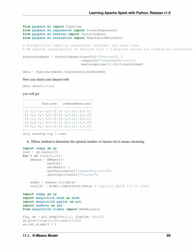
Learning Apache Spark with Python, Release v1.0
from pyspark.ml import Pipelinefrom pyspark.ml.regression import LinearRegressionfrom pyspark.ml.feature import VectorIndexerfrom pyspark.ml.evaluation import RegressionEvaluator
# Automatically identify categorical features, and index them.# We specify maxCategories so features with > 4 distinct values are treated as continuous.
featureIndexer = VectorIndexer(inputCol="features", \outputCol="indexedFeatures",\maxCategories=4).fit(transformed)
data = featureIndexer.transform(transformed)
Now you check your dataset with
data.show(5,True)
you will get
+-----------------+-----------------+| features| indexedFeatures|+-----------------+-----------------+|[5.1,3.5,1.4,0.2]|[5.1,3.5,1.4,0.2]||[4.9,3.0,1.4,0.2]|[4.9,3.0,1.4,0.2]||[4.7,3.2,1.3,0.2]|[4.7,3.2,1.3,0.2]||[4.6,3.1,1.5,0.2]|[4.6,3.1,1.5,0.2]||[5.0,3.6,1.4,0.2]|[5.0,3.6,1.4,0.2]|+-----------------+-----------------+only showing top 5 rows
6. Elbow method to determine the optimal number of clusters for k-means clustering
import numpy as npcost = np.zeros(20)for k in range(2,20):
kmeans = KMeans()\.setK(k)\.setSeed(1) \.setFeaturesCol("indexedFeatures")\.setPredictionCol("cluster")
model = kmeans.fit(data)cost[k] = model.computeCost(data) # requires Spark 2.0 or later
import numpy as npimport matplotlib.mlab as mlabimport matplotlib.pyplot as pltimport seaborn as sbsfrom matplotlib.ticker import MaxNLocator
fig, ax = plt.subplots(1,1, figsize =(8,6))ax.plot(range(2,20),cost[2:20])ax.set_xlabel(’k’)
11.1. K-Means Model 99
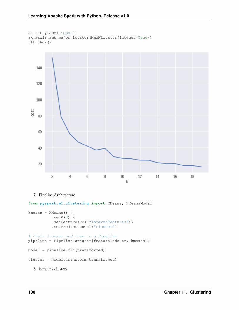
Learning Apache Spark with Python, Release v1.0
ax.set_ylabel(’cost’)ax.xaxis.set_major_locator(MaxNLocator(integer=True))plt.show()
7. Pipeline Architecture
from pyspark.ml.clustering import KMeans, KMeansModel
kmeans = KMeans() \.setK(3) \.setFeaturesCol("indexedFeatures")\.setPredictionCol("cluster")
# Chain indexer and tree in a Pipelinepipeline = Pipeline(stages=[featureIndexer, kmeans])
model = pipeline.fit(transformed)
cluster = model.transform(transformed)
8. k-means clusters
100 Chapter 11. Clustering
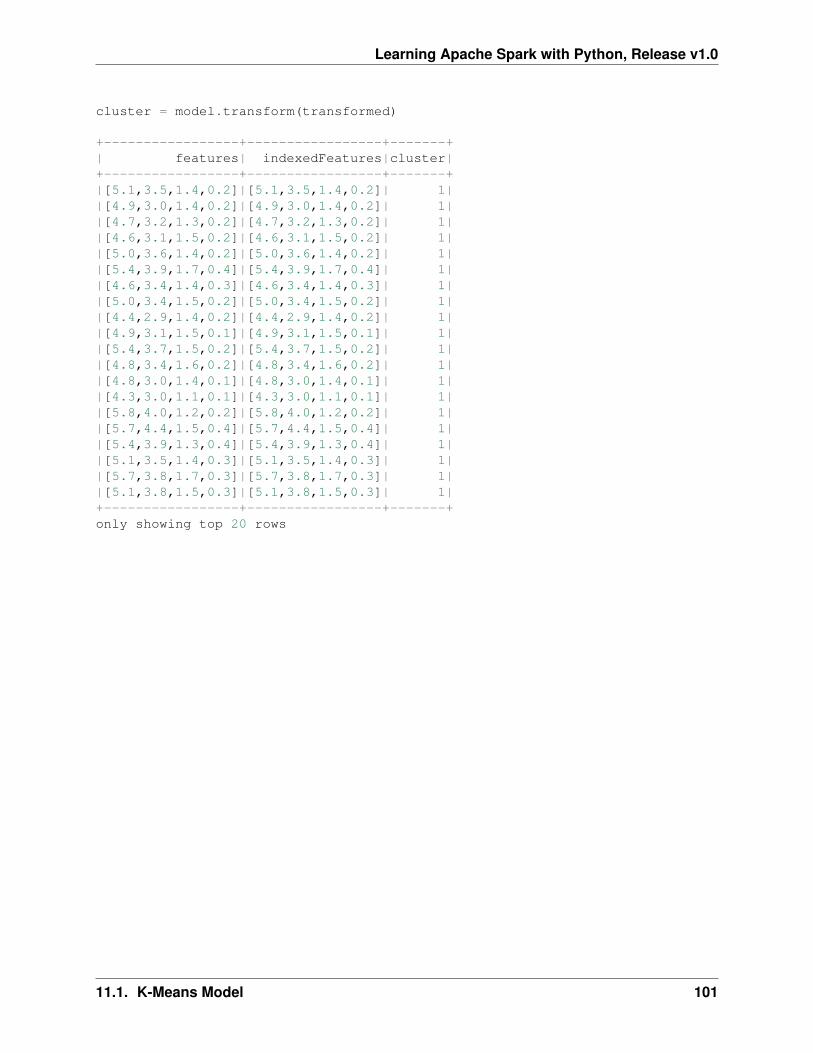
Learning Apache Spark with Python, Release v1.0
cluster = model.transform(transformed)
+-----------------+-----------------+-------+| features| indexedFeatures|cluster|+-----------------+-----------------+-------+|[5.1,3.5,1.4,0.2]|[5.1,3.5,1.4,0.2]| 1||[4.9,3.0,1.4,0.2]|[4.9,3.0,1.4,0.2]| 1||[4.7,3.2,1.3,0.2]|[4.7,3.2,1.3,0.2]| 1||[4.6,3.1,1.5,0.2]|[4.6,3.1,1.5,0.2]| 1||[5.0,3.6,1.4,0.2]|[5.0,3.6,1.4,0.2]| 1||[5.4,3.9,1.7,0.4]|[5.4,3.9,1.7,0.4]| 1||[4.6,3.4,1.4,0.3]|[4.6,3.4,1.4,0.3]| 1||[5.0,3.4,1.5,0.2]|[5.0,3.4,1.5,0.2]| 1||[4.4,2.9,1.4,0.2]|[4.4,2.9,1.4,0.2]| 1||[4.9,3.1,1.5,0.1]|[4.9,3.1,1.5,0.1]| 1||[5.4,3.7,1.5,0.2]|[5.4,3.7,1.5,0.2]| 1||[4.8,3.4,1.6,0.2]|[4.8,3.4,1.6,0.2]| 1||[4.8,3.0,1.4,0.1]|[4.8,3.0,1.4,0.1]| 1||[4.3,3.0,1.1,0.1]|[4.3,3.0,1.1,0.1]| 1||[5.8,4.0,1.2,0.2]|[5.8,4.0,1.2,0.2]| 1||[5.7,4.4,1.5,0.4]|[5.7,4.4,1.5,0.4]| 1||[5.4,3.9,1.3,0.4]|[5.4,3.9,1.3,0.4]| 1||[5.1,3.5,1.4,0.3]|[5.1,3.5,1.4,0.3]| 1||[5.7,3.8,1.7,0.3]|[5.7,3.8,1.7,0.3]| 1||[5.1,3.8,1.5,0.3]|[5.1,3.8,1.5,0.3]| 1|+-----------------+-----------------+-------+only showing top 20 rows
11.1. K-Means Model 101

Learning Apache Spark with Python, Release v1.0
102 Chapter 11. Clustering

CHAPTER
TWELVE
RFM ANALYSIS
RFM is a method used for analyzing customer value. It is commonly used in database marketing and directmarketing and has received particular attention in retail and professional services industries. More detailscan be found at Wikipedia RFM_wikipedia.
RFM stands for the three dimensions:
• Recency – How recently did the customer purchase? i.e. Duration since last purchase
• Frequency – How often do they purchase? i.e. Total number of purchases
• Monetary Value – How much do they spend? i.e. Total money this customer spent
12.1 RFM Analysis Methodology
RFM Analysis contains three main steps:
12.1.1 1. Build the RFM features matrix for each customer
+----------+-------+---------+---------+|CustomerID|Recency|Frequency| Monetary|+----------+-------+---------+---------+| 14911| 1| 248|132572.62|| 12748| 0| 224| 29072.1|| 17841| 1| 169| 40340.78|| 14606| 1| 128| 11713.85|| 15311| 0| 118| 59419.34|+----------+-------+---------+---------+only showing top 5 rows
12.1.2 2. Determine cutting points for each feature
+----------+-------+---------+--------+-----+-----+-----+|CustomerID|Recency|Frequency|Monetary|r_seg|f_seg|m_seg|+----------+-------+---------+--------+-----+-----+-----+| 17420| 50| 3| 598.83| 2| 3| 2|| 16861| 59| 3| 151.65| 3| 3| 1|
103
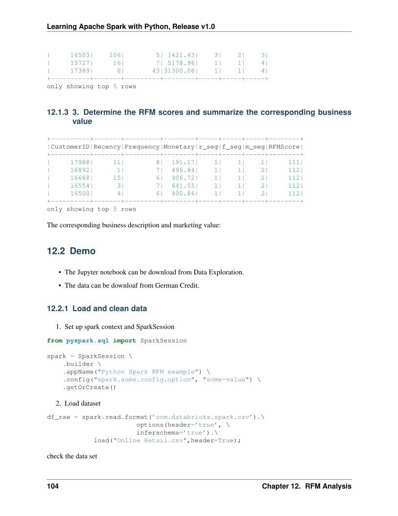
Learning Apache Spark with Python, Release v1.0
| 16503| 106| 5| 1421.43| 3| 2| 3|| 15727| 16| 7| 5178.96| 1| 1| 4|| 17389| 0| 43|31300.08| 1| 1| 4|+----------+-------+---------+--------+-----+-----+-----+only showing top 5 rows
12.1.3 3. Determine the RFM scores and summarize the corresponding businessvalue
+----------+-------+---------+--------+-----+-----+-----+--------+|CustomerID|Recency|Frequency|Monetary|r_seg|f_seg|m_seg|RFMScore|+----------+-------+---------+--------+-----+-----+-----+--------+| 17988| 11| 8| 191.17| 1| 1| 1| 111|| 16892| 1| 7| 496.84| 1| 1| 2| 112|| 16668| 15| 6| 306.72| 1| 1| 2| 112|| 16554| 3| 7| 641.55| 1| 1| 2| 112|| 16500| 4| 6| 400.86| 1| 1| 2| 112|+----------+-------+---------+--------+-----+-----+-----+--------+only showing top 5 rows
The corresponding business description and marketing value:
12.2 Demo
• The Jupyter notebook can be download from Data Exploration.
• The data can be downloaf from German Credit.
12.2.1 Load and clean data
1. Set up spark context and SparkSession
from pyspark.sql import SparkSession
spark = SparkSession \.builder \.appName("Python Spark RFM example") \.config("spark.some.config.option", "some-value") \.getOrCreate()
2. Load dataset
df_raw = spark.read.format(’com.databricks.spark.csv’).\options(header=’true’, \inferschema=’true’).\
load("Online Retail.csv",header=True);
check the data set
104 Chapter 12. RFM Analysis
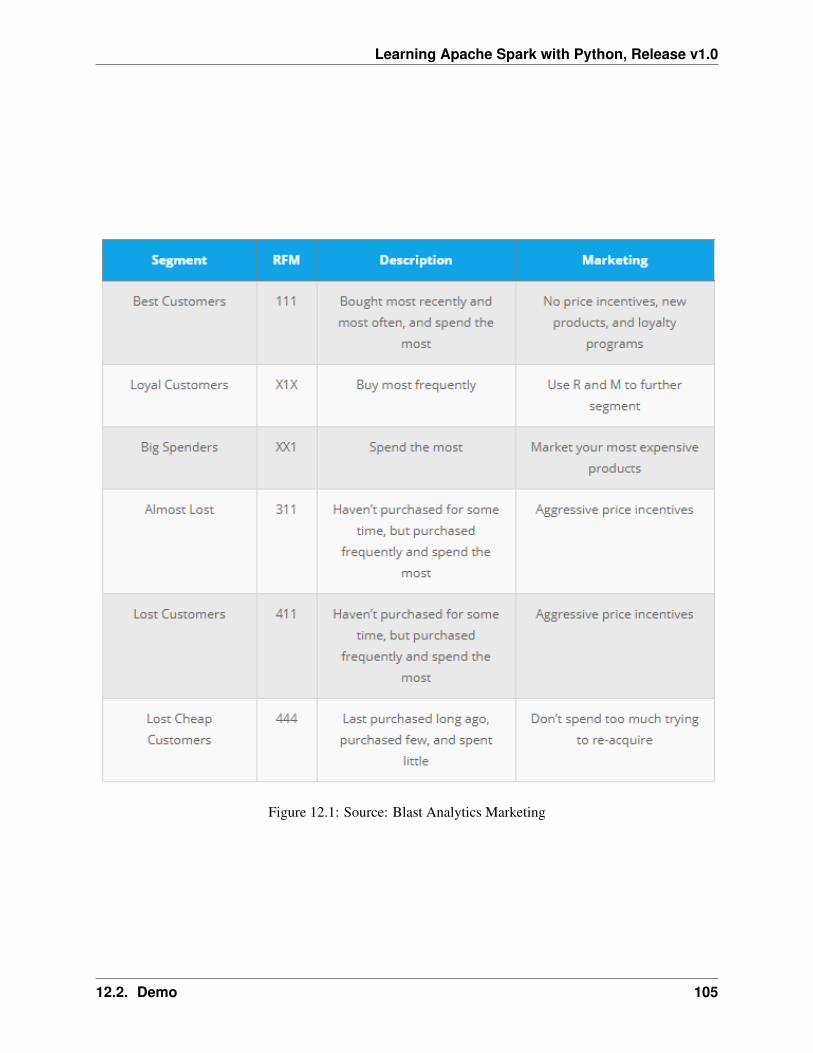
Learning Apache Spark with Python, Release v1.0
Figure 12.1: Source: Blast Analytics Marketing
12.2. Demo 105
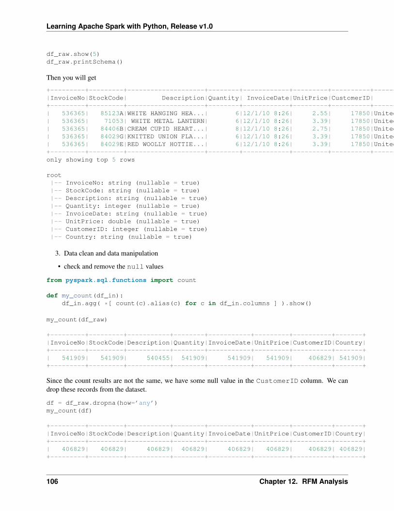
Learning Apache Spark with Python, Release v1.0
df_raw.show(5)df_raw.printSchema()
Then you will get
+---------+---------+--------------------+--------+------------+---------+----------+--------------+|InvoiceNo|StockCode| Description|Quantity| InvoiceDate|UnitPrice|CustomerID| Country|+---------+---------+--------------------+--------+------------+---------+----------+--------------+| 536365| 85123A|WHITE HANGING HEA...| 6|12/1/10 8:26| 2.55| 17850|United Kingdom|| 536365| 71053| WHITE METAL LANTERN| 6|12/1/10 8:26| 3.39| 17850|United Kingdom|| 536365| 84406B|CREAM CUPID HEART...| 8|12/1/10 8:26| 2.75| 17850|United Kingdom|| 536365| 84029G|KNITTED UNION FLA...| 6|12/1/10 8:26| 3.39| 17850|United Kingdom|| 536365| 84029E|RED WOOLLY HOTTIE...| 6|12/1/10 8:26| 3.39| 17850|United Kingdom|+---------+---------+--------------------+--------+------------+---------+----------+--------------+only showing top 5 rows
root|-- InvoiceNo: string (nullable = true)|-- StockCode: string (nullable = true)|-- Description: string (nullable = true)|-- Quantity: integer (nullable = true)|-- InvoiceDate: string (nullable = true)|-- UnitPrice: double (nullable = true)|-- CustomerID: integer (nullable = true)|-- Country: string (nullable = true)
3. Data clean and data manipulation
• check and remove the null values
from pyspark.sql.functions import count
def my_count(df_in):df_in.agg( *[ count(c).alias(c) for c in df_in.columns ] ).show()
my_count(df_raw)
+---------+---------+-----------+--------+-----------+---------+----------+-------+|InvoiceNo|StockCode|Description|Quantity|InvoiceDate|UnitPrice|CustomerID|Country|+---------+---------+-----------+--------+-----------+---------+----------+-------+| 541909| 541909| 540455| 541909| 541909| 541909| 406829| 541909|+---------+---------+-----------+--------+-----------+---------+----------+-------+
Since the count results are not the same, we have some null value in the CustomerID column. We candrop these records from the dataset.
df = df_raw.dropna(how=’any’)my_count(df)
+---------+---------+-----------+--------+-----------+---------+----------+-------+|InvoiceNo|StockCode|Description|Quantity|InvoiceDate|UnitPrice|CustomerID|Country|+---------+---------+-----------+--------+-----------+---------+----------+-------+| 406829| 406829| 406829| 406829| 406829| 406829| 406829| 406829|+---------+---------+-----------+--------+-----------+---------+----------+-------+
106 Chapter 12. RFM Analysis
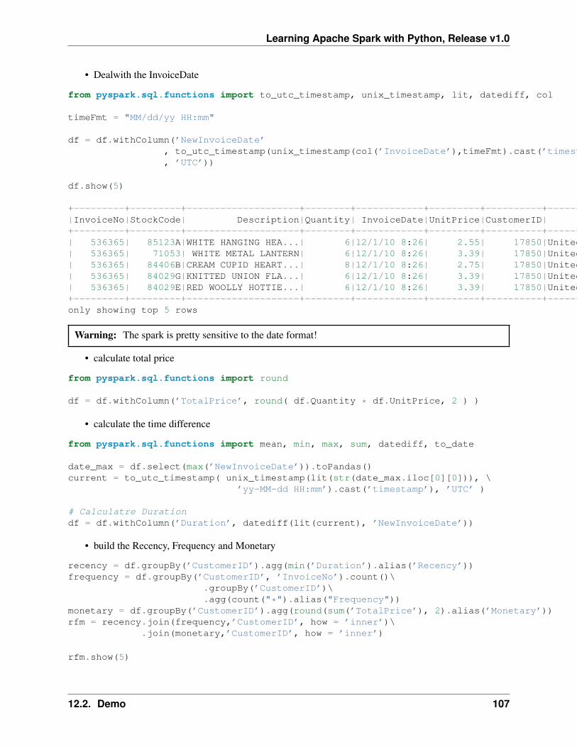
Learning Apache Spark with Python, Release v1.0
• Dealwith the InvoiceDate
from pyspark.sql.functions import to_utc_timestamp, unix_timestamp, lit, datediff, col
timeFmt = "MM/dd/yy HH:mm"
df = df.withColumn(’NewInvoiceDate’, to_utc_timestamp(unix_timestamp(col(’InvoiceDate’),timeFmt).cast(’timestamp’), ’UTC’))
df.show(5)
+---------+---------+--------------------+--------+------------+---------+----------+--------------+--------------------+|InvoiceNo|StockCode| Description|Quantity| InvoiceDate|UnitPrice|CustomerID| Country| NewInvoiceDate|+---------+---------+--------------------+--------+------------+---------+----------+--------------+--------------------+| 536365| 85123A|WHITE HANGING HEA...| 6|12/1/10 8:26| 2.55| 17850|United Kingdom|2010-12-01 08:26:...|| 536365| 71053| WHITE METAL LANTERN| 6|12/1/10 8:26| 3.39| 17850|United Kingdom|2010-12-01 08:26:...|| 536365| 84406B|CREAM CUPID HEART...| 8|12/1/10 8:26| 2.75| 17850|United Kingdom|2010-12-01 08:26:...|| 536365| 84029G|KNITTED UNION FLA...| 6|12/1/10 8:26| 3.39| 17850|United Kingdom|2010-12-01 08:26:...|| 536365| 84029E|RED WOOLLY HOTTIE...| 6|12/1/10 8:26| 3.39| 17850|United Kingdom|2010-12-01 08:26:...|+---------+---------+--------------------+--------+------------+---------+----------+--------------+--------------------+only showing top 5 rows
Warning: The spark is pretty sensitive to the date format!
• calculate total price
from pyspark.sql.functions import round
df = df.withColumn(’TotalPrice’, round( df.Quantity * df.UnitPrice, 2 ) )
• calculate the time difference
from pyspark.sql.functions import mean, min, max, sum, datediff, to_date
date_max = df.select(max(’NewInvoiceDate’)).toPandas()current = to_utc_timestamp( unix_timestamp(lit(str(date_max.iloc[0][0])), \
’yy-MM-dd HH:mm’).cast(’timestamp’), ’UTC’ )
# Calculatre Durationdf = df.withColumn(’Duration’, datediff(lit(current), ’NewInvoiceDate’))
• build the Recency, Frequency and Monetary
recency = df.groupBy(’CustomerID’).agg(min(’Duration’).alias(’Recency’))frequency = df.groupBy(’CustomerID’, ’InvoiceNo’).count()\
.groupBy(’CustomerID’)\
.agg(count("*").alias("Frequency"))monetary = df.groupBy(’CustomerID’).agg(round(sum(’TotalPrice’), 2).alias(’Monetary’))rfm = recency.join(frequency,’CustomerID’, how = ’inner’)\
.join(monetary,’CustomerID’, how = ’inner’)
rfm.show(5)
12.2. Demo 107
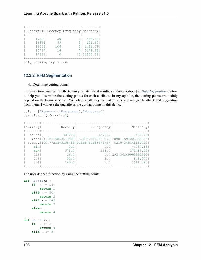
Learning Apache Spark with Python, Release v1.0
+----------+-------+---------+--------+|CustomerID|Recency|Frequency|Monetary|+----------+-------+---------+--------+| 17420| 50| 3| 598.83|| 16861| 59| 3| 151.65|| 16503| 106| 5| 1421.43|| 15727| 16| 7| 5178.96|| 17389| 0| 43|31300.08|+----------+-------+---------+--------+only showing top 5 rows
12.2.2 RFM Segmentation
4. Determine cutting points
In this section, you can use the techniques (statistical results and visualizations) in Data Exploration sectionto help you determine the cutting points for each attribute. In my opinion, the cutting points are mainlydepend on the business sense. You’s better talk to your makrting people and get feedback and suggestionfrom them. I will use the quantile as the cutting points in this demo.
cols = [’Recency’,’Frequency’,’Monetary’]describe_pd(rfm,cols,1)
+-------+-----------------+-----------------+------------------+|summary| Recency| Frequency| Monetary|+-------+-----------------+-----------------+------------------+| count| 4372.0| 4372.0| 4372.0|| mean|91.58119853613907| 5.07548032936871|1898.4597003659655|| stddev|100.7721393138483|9.338754163574727| 8219.345141139722|| min| 0.0| 1.0| -4287.63|| max| 373.0| 248.0| 279489.02|| 25%| 16.0| 1.0|293.36249999999995|| 50%| 50.0| 3.0| 648.075|| 75%| 143.0| 5.0| 1611.725|+-------+-----------------+-----------------+------------------+
The user defined function by using the cutting points:
def RScore(x):if x <= 16:
return 1elif x<= 50:
return 2elif x<= 143:
return 3else:
return 4
def FScore(x):if x <= 1:
return 4elif x <= 3:
108 Chapter 12. RFM Analysis
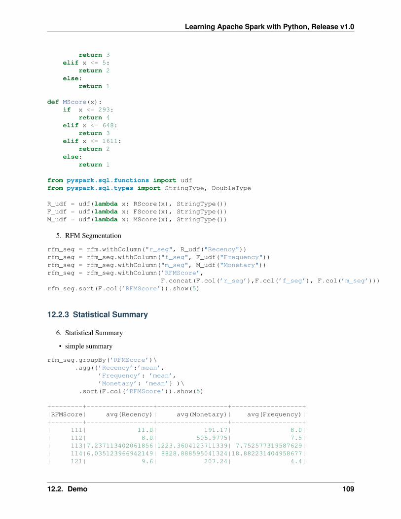
Learning Apache Spark with Python, Release v1.0
return 3elif x <= 5:
return 2else:
return 1
def MScore(x):if x <= 293:
return 4elif x <= 648:
return 3elif x <= 1611:
return 2else:
return 1
from pyspark.sql.functions import udffrom pyspark.sql.types import StringType, DoubleType
R_udf = udf(lambda x: RScore(x), StringType())F_udf = udf(lambda x: FScore(x), StringType())M_udf = udf(lambda x: MScore(x), StringType())
5. RFM Segmentation
rfm_seg = rfm.withColumn("r_seg", R_udf("Recency"))rfm_seg = rfm_seg.withColumn("f_seg", F_udf("Frequency"))rfm_seg = rfm_seg.withColumn("m_seg", M_udf("Monetary"))rfm_seg = rfm_seg.withColumn(’RFMScore’,
F.concat(F.col(’r_seg’),F.col(’f_seg’), F.col(’m_seg’)))rfm_seg.sort(F.col(’RFMScore’)).show(5)
12.2.3 Statistical Summary
6. Statistical Summary
• simple summary
rfm_seg.groupBy(’RFMScore’)\.agg({’Recency’:’mean’,
’Frequency’: ’mean’,’Monetary’: ’mean’} )\
.sort(F.col(’RFMScore’)).show(5)
+--------+-----------------+------------------+------------------+|RFMScore| avg(Recency)| avg(Monetary)| avg(Frequency)|+--------+-----------------+------------------+------------------+| 111| 11.0| 191.17| 8.0|| 112| 8.0| 505.9775| 7.5|| 113|7.237113402061856|1223.3604123711339| 7.752577319587629|| 114|6.035123966942149| 8828.888595041324|18.882231404958677|| 121| 9.6| 207.24| 4.4|
12.2. Demo 109
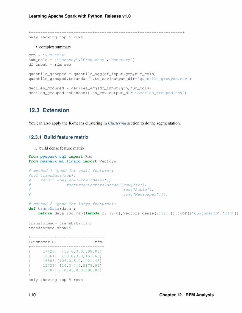
Learning Apache Spark with Python, Release v1.0
+--------+-----------------+------------------+------------------+only showing top 5 rows
• complex summary
grp = ’RFMScore’num_cols = [’Recency’,’Frequency’,’Monetary’]df_input = rfm_seg
quantile_grouped = quantile_agg(df_input,grp,num_cols)quantile_grouped.toPandas().to_csv(output_dir+’quantile_grouped.csv’)
deciles_grouped = deciles_agg(df_input,grp,num_cols)deciles_grouped.toPandas().to_csv(output_dir+’deciles_grouped.csv’)
12.3 Extension
You can also apply the K-means clustering in Clustering section to do the segmentation.
12.3.1 Build feature matrix
1. build dense feature matrix
from pyspark.sql import Rowfrom pyspark.ml.linalg import Vectors
# method 1 (good for small feature):#def transData(row):# return Row(label=row["Sales"],# features=Vectors.dense([row["TV"],# row["Radio"],# row["Newspaper"]]))
# Method 2 (good for large features):def transData(data):
return data.rdd.map(lambda r: [r[0],Vectors.dense(r[1:])]).toDF([’CustomerID’,’rfm’])
transformed= transData(rfm)transformed.show(5)
+----------+-------------------+|CustomerID| rfm|+----------+-------------------+| 17420| [50.0,3.0,598.83]|| 16861| [59.0,3.0,151.65]|| 16503|[106.0,5.0,1421.43]|| 15727| [16.0,7.0,5178.96]|| 17389|[0.0,43.0,31300.08]|+----------+-------------------+only showing top 5 rows
110 Chapter 12. RFM Analysis

Learning Apache Spark with Python, Release v1.0
2. Scaler the feature matrix
from pyspark.ml.feature import MinMaxScaler
scaler = MinMaxScaler(inputCol="rfm",\outputCol="features")
scalerModel = scaler.fit(transformed)scaledData = scalerModel.transform(transformed)scaledData.show(5,False)
+----------+-------------------+--------------------------------------------------------------+|CustomerID|rfm |features |+----------+-------------------+--------------------------------------------------------------+|17420 |[50.0,3.0,598.83] |[0.13404825737265416,0.008097165991902834,0.01721938714830836]||16861 |[59.0,3.0,151.65] |[0.1581769436997319,0.008097165991902834,0.01564357039241953] ||16503 |[106.0,5.0,1421.43]|[0.28418230563002683,0.016194331983805668,0.02011814573186342]||15727 |[16.0,7.0,5178.96] |[0.04289544235924933,0.024291497975708502,0.03335929858922501]||17389 |[0.0,43.0,31300.08]|[0.0,0.1700404858299595,0.12540746393334334] |+----------+-------------------+--------------------------------------------------------------+only showing top 5 rows
12.3.2 K-means clustering
3. Find optimal number of cluster
I will present two popular ways to determine the optimal number of the cluster.
• elbow analysis
#PySpark librariesfrom pyspark.ml import Pipelinefrom pyspark.ml.feature import StringIndexer, OneHotEncoder, VectorAssemblerfrom pyspark.sql.functions import col, percent_rank, litfrom pyspark.sql.window import Windowfrom pyspark.sql import DataFrame, Rowfrom pyspark.sql.types import StructTypefrom functools import reduce # For Python 3.x
from pyspark.ml.clustering import KMeans#from pyspark.ml.evaluation import ClusteringEvaluator # requires Spark 2.4 or later
import numpy as npcost = np.zeros(20)for k in range(2,20):
kmeans = KMeans()\.setK(k)\.setSeed(1) \.setFeaturesCol("features")\.setPredictionCol("cluster")
model = kmeans.fit(scaledData)cost[k] = model.computeCost(scaledData) # requires Spark 2.0 or later
12.3. Extension 111
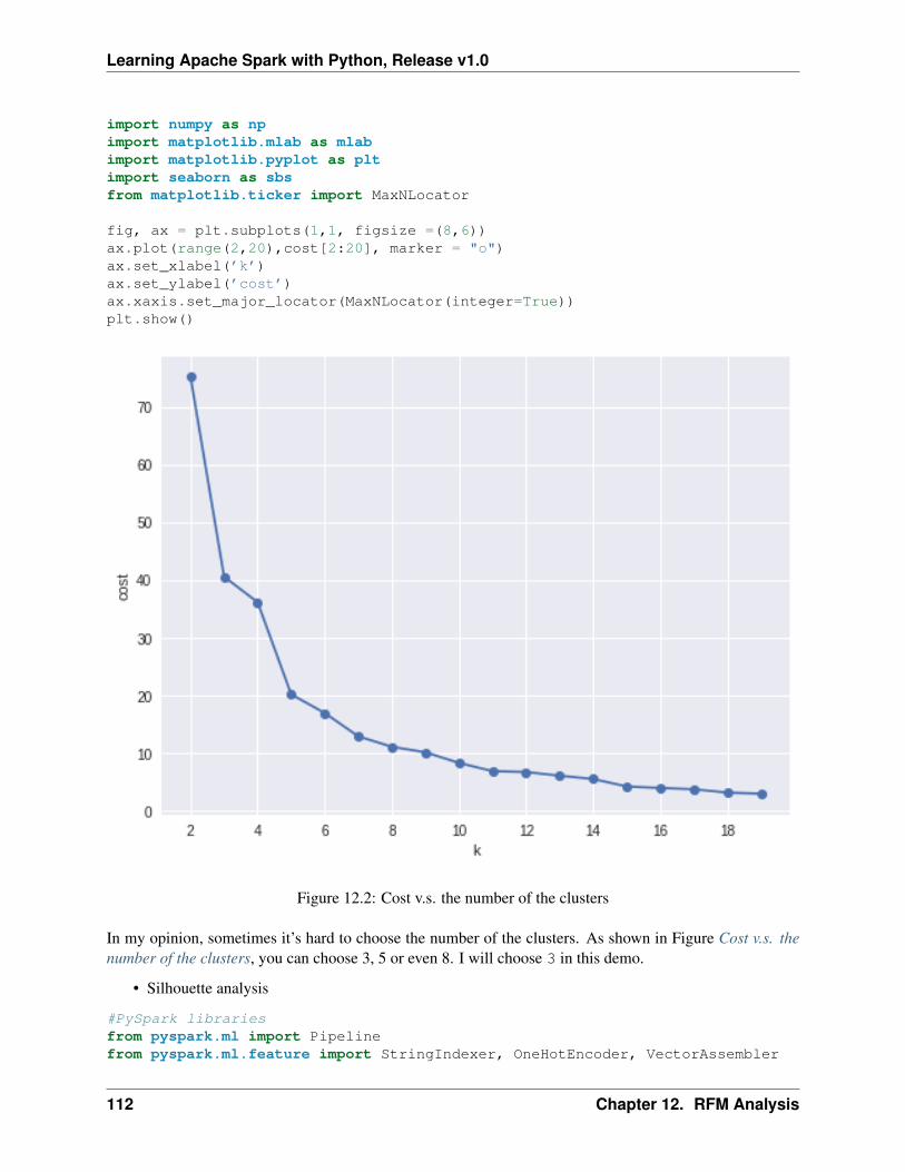
Learning Apache Spark with Python, Release v1.0
import numpy as npimport matplotlib.mlab as mlabimport matplotlib.pyplot as pltimport seaborn as sbsfrom matplotlib.ticker import MaxNLocator
fig, ax = plt.subplots(1,1, figsize =(8,6))ax.plot(range(2,20),cost[2:20], marker = "o")ax.set_xlabel(’k’)ax.set_ylabel(’cost’)ax.xaxis.set_major_locator(MaxNLocator(integer=True))plt.show()
Figure 12.2: Cost v.s. the number of the clusters
In my opinion, sometimes it’s hard to choose the number of the clusters. As shown in Figure Cost v.s. thenumber of the clusters, you can choose 3, 5 or even 8. I will choose 3 in this demo.
• Silhouette analysis
#PySpark librariesfrom pyspark.ml import Pipelinefrom pyspark.ml.feature import StringIndexer, OneHotEncoder, VectorAssembler
112 Chapter 12. RFM Analysis
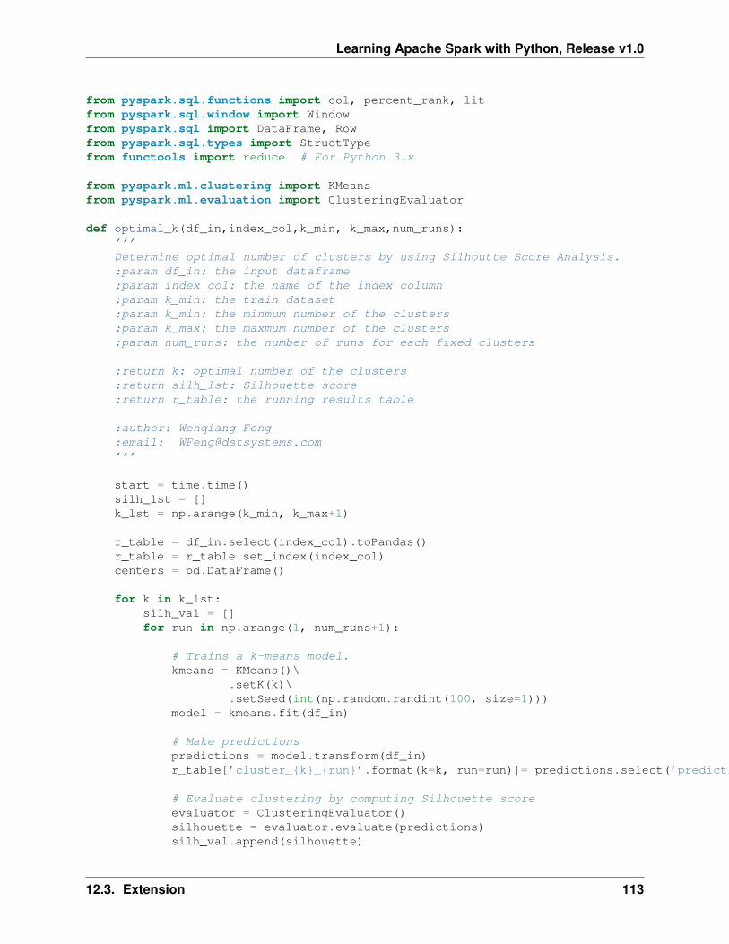
Learning Apache Spark with Python, Release v1.0
from pyspark.sql.functions import col, percent_rank, litfrom pyspark.sql.window import Windowfrom pyspark.sql import DataFrame, Rowfrom pyspark.sql.types import StructTypefrom functools import reduce # For Python 3.x
from pyspark.ml.clustering import KMeansfrom pyspark.ml.evaluation import ClusteringEvaluator
def optimal_k(df_in,index_col,k_min, k_max,num_runs):’’’Determine optimal number of clusters by using Silhoutte Score Analysis.:param df_in: the input dataframe:param index_col: the name of the index column:param k_min: the train dataset:param k_min: the minmum number of the clusters:param k_max: the maxmum number of the clusters:param num_runs: the number of runs for each fixed clusters
:return k: optimal number of the clusters:return silh_lst: Silhouette score:return r_table: the running results table
:author: Wenqiang Feng:email: [email protected]’’’
start = time.time()silh_lst = []k_lst = np.arange(k_min, k_max+1)
r_table = df_in.select(index_col).toPandas()r_table = r_table.set_index(index_col)centers = pd.DataFrame()
for k in k_lst:silh_val = []for run in np.arange(1, num_runs+1):
# Trains a k-means model.kmeans = KMeans()\
.setK(k)\
.setSeed(int(np.random.randint(100, size=1)))model = kmeans.fit(df_in)
# Make predictionspredictions = model.transform(df_in)r_table[’cluster_{k}_{run}’.format(k=k, run=run)]= predictions.select(’prediction’).toPandas()
# Evaluate clustering by computing Silhouette scoreevaluator = ClusteringEvaluator()silhouette = evaluator.evaluate(predictions)silh_val.append(silhouette)
12.3. Extension 113
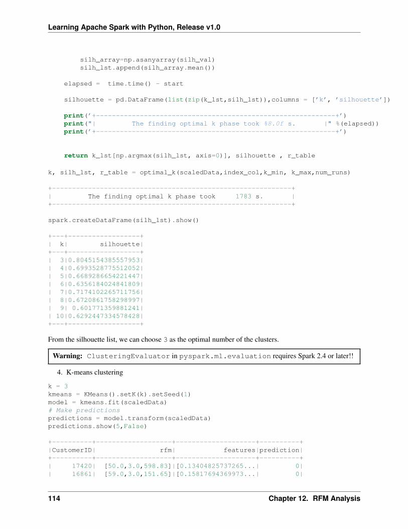
Learning Apache Spark with Python, Release v1.0
silh_array=np.asanyarray(silh_val)silh_lst.append(silh_array.mean())
elapsed = time.time() - start
silhouette = pd.DataFrame(list(zip(k_lst,silh_lst)),columns = [’k’, ’silhouette’])
print(’+------------------------------------------------------------+’)print("| The finding optimal k phase took %8.0f s. |" %(elapsed))print(’+------------------------------------------------------------+’)
return k_lst[np.argmax(silh_lst, axis=0)], silhouette , r_table
k, silh_lst, r_table = optimal_k(scaledData,index_col,k_min, k_max,num_runs)
+------------------------------------------------------------+| The finding optimal k phase took 1783 s. |+------------------------------------------------------------+
spark.createDataFrame(silh_lst).show()
+---+------------------+| k| silhouette|+---+------------------+| 3|0.8045154385557953|| 4|0.6993528775512052|| 5|0.6689286654221447|| 6|0.6356184024841809|| 7|0.7174102265711756|| 8|0.6720861758298997|| 9| 0.601771359881241|| 10|0.6292447334578428|+---+------------------+
From the silhouette list, we can choose 3 as the optimal number of the clusters.
Warning: ClusteringEvaluator in pyspark.ml.evaluation requires Spark 2.4 or later!!
4. K-means clustering
k = 3kmeans = KMeans().setK(k).setSeed(1)model = kmeans.fit(scaledData)# Make predictionspredictions = model.transform(scaledData)predictions.show(5,False)
+----------+-------------------+--------------------+----------+|CustomerID| rfm| features|prediction|+----------+-------------------+--------------------+----------+| 17420| [50.0,3.0,598.83]|[0.13404825737265...| 0|| 16861| [59.0,3.0,151.65]|[0.15817694369973...| 0|
114 Chapter 12. RFM Analysis
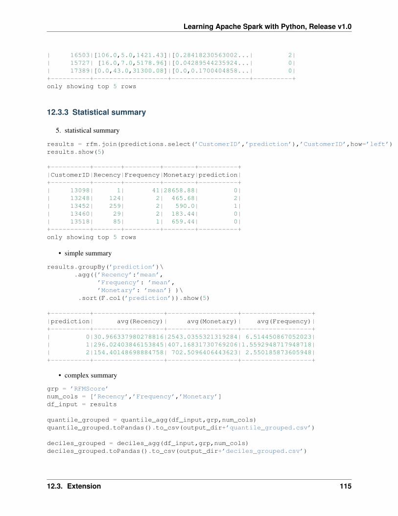
Learning Apache Spark with Python, Release v1.0
| 16503|[106.0,5.0,1421.43]|[0.28418230563002...| 2|| 15727| [16.0,7.0,5178.96]|[0.04289544235924...| 0|| 17389|[0.0,43.0,31300.08]|[0.0,0.1700404858...| 0|+----------+-------------------+--------------------+----------+only showing top 5 rows
12.3.3 Statistical summary
5. statistical summary
results = rfm.join(predictions.select(’CustomerID’,’prediction’),’CustomerID’,how=’left’)results.show(5)
+----------+-------+---------+--------+----------+|CustomerID|Recency|Frequency|Monetary|prediction|+----------+-------+---------+--------+----------+| 13098| 1| 41|28658.88| 0|| 13248| 124| 2| 465.68| 2|| 13452| 259| 2| 590.0| 1|| 13460| 29| 2| 183.44| 0|| 13518| 85| 1| 659.44| 0|+----------+-------+---------+--------+----------+only showing top 5 rows
• simple summary
results.groupBy(’prediction’)\.agg({’Recency’:’mean’,
’Frequency’: ’mean’,’Monetary’: ’mean’} )\
.sort(F.col(’prediction’)).show(5)
+----------+------------------+------------------+------------------+|prediction| avg(Recency)| avg(Monetary)| avg(Frequency)|+----------+------------------+------------------+------------------+| 0|30.966337980278816|2543.0355321319284| 6.514450867052023|| 1|296.02403846153845|407.16831730769206|1.5592948717948718|| 2|154.40148698884758| 702.5096406443623| 2.550185873605948|+----------+------------------+------------------+------------------+
• complex summary
grp = ’RFMScore’num_cols = [’Recency’,’Frequency’,’Monetary’]df_input = results
quantile_grouped = quantile_agg(df_input,grp,num_cols)quantile_grouped.toPandas().to_csv(output_dir+’quantile_grouped.csv’)
deciles_grouped = deciles_agg(df_input,grp,num_cols)deciles_grouped.toPandas().to_csv(output_dir+’deciles_grouped.csv’)
12.3. Extension 115

Learning Apache Spark with Python, Release v1.0
116 Chapter 12. RFM Analysis
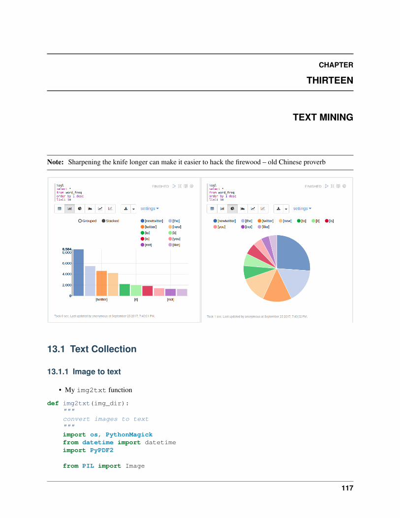
CHAPTER
THIRTEEN
TEXT MINING
Note: Sharpening the knife longer can make it easier to hack the firewood – old Chinese proverb
13.1 Text Collection
13.1.1 Image to text
• My img2txt function
def img2txt(img_dir):"""convert images to text"""import os, PythonMagickfrom datetime import datetimeimport PyPDF2
from PIL import Image
117

Learning Apache Spark with Python, Release v1.0
import pytesseract
f = open(’doc4img.txt’,’wa’)for img in [img_file for img_file in os.listdir(img_dir)
if (img_file.endswith(".png") orimg_file.endswith(".jpg") orimg_file.endswith(".jpeg"))]:
start_time = datetime.now()
input_img = img_dir + "/" + img
print(’--------------------------------------------------------------------’)print(img)print(’Converting ’ + img +’.......’)print(’--------------------------------------------------------------------’)
# extract the text information from imagestext = pytesseract.image_to_string(Image.open(input_img))print(text)
# ouput text filef.write( img + "\n")f.write(text.encode(’utf-8’))
print "CPU Time for converting" + img +":"+ str(datetime.now() - start_time) +"\n"f.write( "\n-------------------------------------------------------------\n")
f.close()
• Demo
I applied my img2txt function to the image in Image folder.
image_dir = r"Image"
img2txt(image_dir)
Then I got the following results:
--------------------------------------------------------------------feng.pdf_0.pngConverting feng.pdf_0.png.......--------------------------------------------------------------------l I l w
Wenqiang FengData ScientistDST APPLIED ANALYTICS GROUP
Wenqiang Feng is Data Scientist for DST’s Applied Analytics Group. Dr. Feng’s responsibilities
118 Chapter 13. Text Mining
Learning Apache Spark with Python, Release v1.0
include providing DST clients with access to cutting--edge skills and technologies, including BigData analytic solutions, advanced analytic and data enhancement techniques and modeling.
Dr. Feng has deep analytic expertise in data mining, analytic systems, machine learningalgorithms, business intelligence, and applying Big Data tools to strategically solve industryproblems in a cross--functional business. Before joining the DST Applied Analytics Group, Dr.Feng holds a MA Data Science Fellow at The Institute for Mathematics and Its Applications{IMA) at the University of Minnesota. While there, he helped startup companies makemarketing decisions based on deep predictive analytics.
Dr. Feng graduated from University of Tennessee, Knoxville with PhD in Computationalmathematics and Master’s degree in Statistics. He also holds Master’s degree in ComputationalMathematics at Missouri University of Science and Technology (MST) and Master’s degree inApplied Mathematics at University of science and technology of China (USTC).CPU Time for convertingfeng.pdf_0.png:0:00:02.061208
13.1.2 Image Enhnaced to text
• My img2txt_enhance function
def img2txt_enhance(img_dir,scaler):"""convert images files to text"""
import numpy as npimport os, PythonMagickfrom datetime import datetimeimport PyPDF2
from PIL import Image, ImageEnhance, ImageFilterimport pytesseract
f = open(’doc4img.txt’,’wa’)for img in [img_file for img_file in os.listdir(img_dir)
if (img_file.endswith(".png") orimg_file.endswith(".jpg") orimg_file.endswith(".jpeg"))]:
start_time = datetime.now()
input_img = img_dir + "/" + imgenhanced_img = img_dir + "/" +"Enhanced" + "/"+ img
im = Image.open(input_img) # the second oneim = im.filter(ImageFilter.MedianFilter())enhancer = ImageEnhance.Contrast(im)im = enhancer.enhance(1)im = im.convert(’1’)im.save(enhanced_img)
for scale in np.ones(scaler):
13.1. Text Collection 119
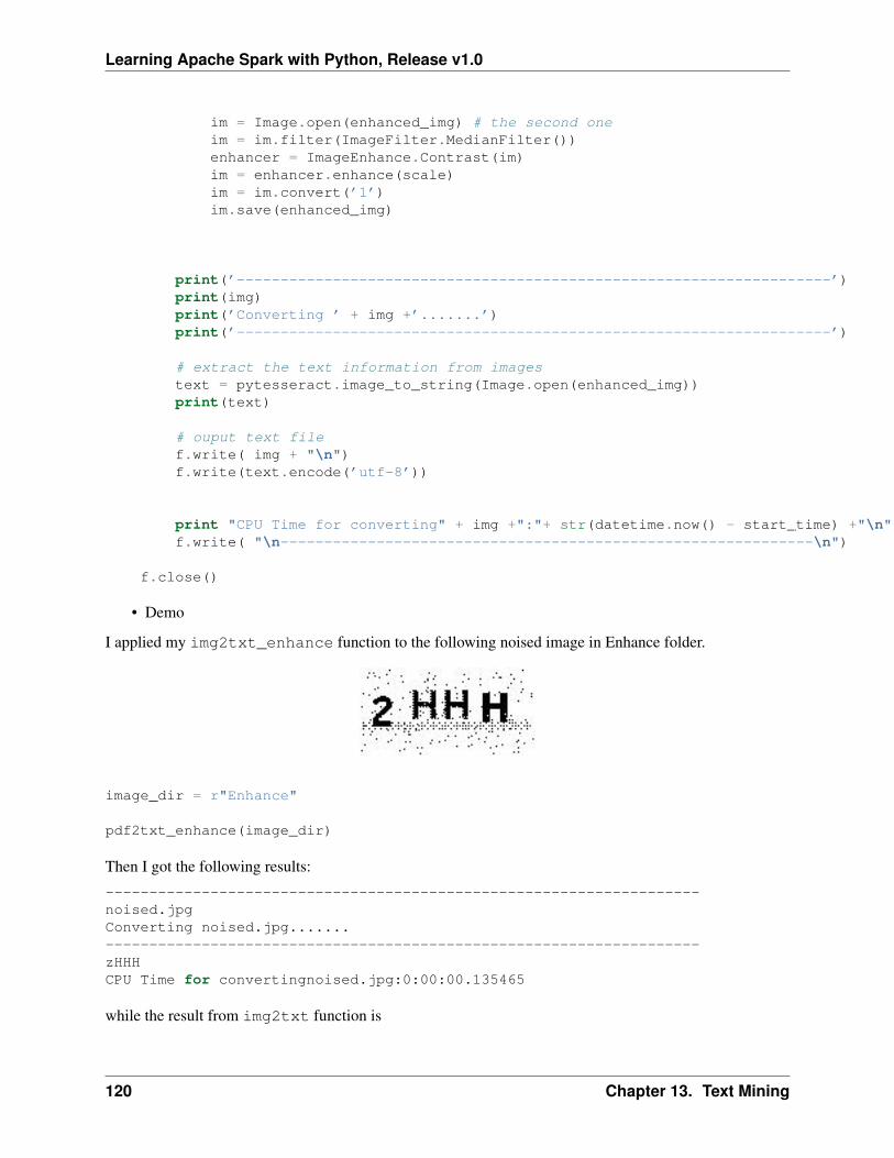
Learning Apache Spark with Python, Release v1.0
im = Image.open(enhanced_img) # the second oneim = im.filter(ImageFilter.MedianFilter())enhancer = ImageEnhance.Contrast(im)im = enhancer.enhance(scale)im = im.convert(’1’)im.save(enhanced_img)
print(’--------------------------------------------------------------------’)print(img)print(’Converting ’ + img +’.......’)print(’--------------------------------------------------------------------’)
# extract the text information from imagestext = pytesseract.image_to_string(Image.open(enhanced_img))print(text)
# ouput text filef.write( img + "\n")f.write(text.encode(’utf-8’))
print "CPU Time for converting" + img +":"+ str(datetime.now() - start_time) +"\n"f.write( "\n-------------------------------------------------------------\n")
f.close()
• Demo
I applied my img2txt_enhance function to the following noised image in Enhance folder.
image_dir = r"Enhance"
pdf2txt_enhance(image_dir)
Then I got the following results:
--------------------------------------------------------------------noised.jpgConverting noised.jpg.......--------------------------------------------------------------------zHHHCPU Time for convertingnoised.jpg:0:00:00.135465
while the result from img2txt function is
120 Chapter 13. Text Mining
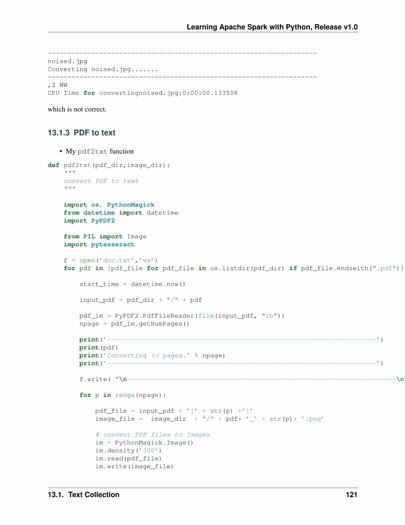
Learning Apache Spark with Python, Release v1.0
--------------------------------------------------------------------noised.jpgConverting noised.jpg.......--------------------------------------------------------------------,2 WWCPU Time for convertingnoised.jpg:0:00:00.133508
which is not correct.
13.1.3 PDF to text
• My pdf2txt function
def pdf2txt(pdf_dir,image_dir):"""convert PDF to text"""
import os, PythonMagickfrom datetime import datetimeimport PyPDF2
from PIL import Imageimport pytesseract
f = open(’doc.txt’,’wa’)for pdf in [pdf_file for pdf_file in os.listdir(pdf_dir) if pdf_file.endswith(".pdf")]:
start_time = datetime.now()
input_pdf = pdf_dir + "/" + pdf
pdf_im = PyPDF2.PdfFileReader(file(input_pdf, "rb"))npage = pdf_im.getNumPages()
print(’--------------------------------------------------------------------’)print(pdf)print(’Converting %d pages.’ % npage)print(’--------------------------------------------------------------------’)
f.write( "\n--------------------------------------------------------------------\n")
for p in range(npage):
pdf_file = input_pdf + ’[’ + str(p) +’]’image_file = image_dir + "/" + pdf+ ’_’ + str(p)+ ’.png’
# convert PDF files to Imagesim = PythonMagick.Image()im.density(’300’)im.read(pdf_file)im.write(image_file)
13.1. Text Collection 121
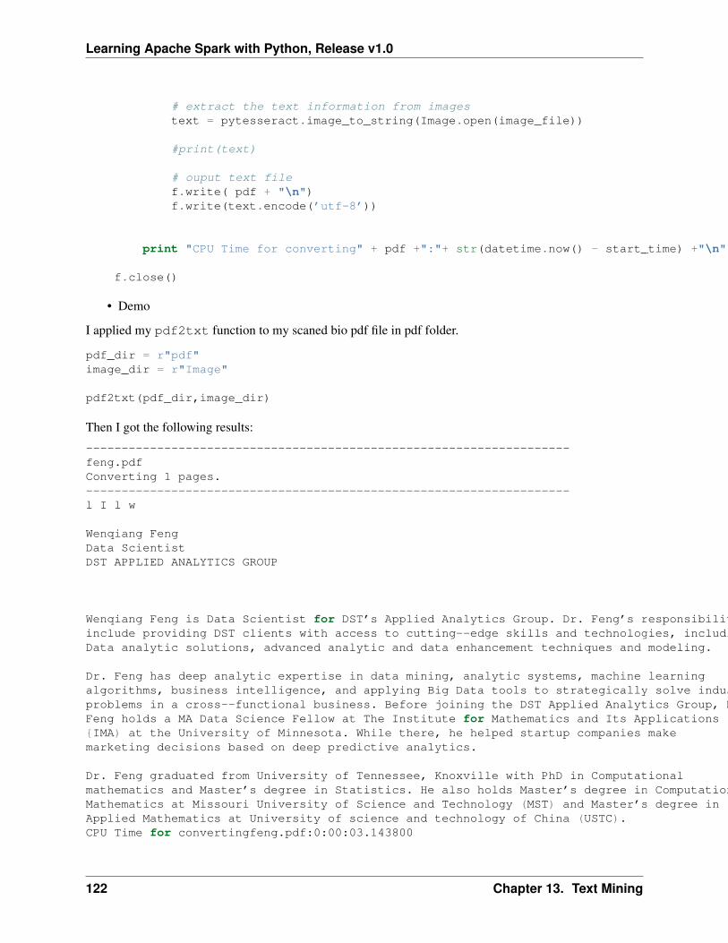
Learning Apache Spark with Python, Release v1.0
# extract the text information from imagestext = pytesseract.image_to_string(Image.open(image_file))
#print(text)
# ouput text filef.write( pdf + "\n")f.write(text.encode(’utf-8’))
print "CPU Time for converting" + pdf +":"+ str(datetime.now() - start_time) +"\n"
f.close()
• Demo
I applied my pdf2txt function to my scaned bio pdf file in pdf folder.
pdf_dir = r"pdf"image_dir = r"Image"
pdf2txt(pdf_dir,image_dir)
Then I got the following results:
--------------------------------------------------------------------feng.pdfConverting 1 pages.--------------------------------------------------------------------l I l w
Wenqiang FengData ScientistDST APPLIED ANALYTICS GROUP
Wenqiang Feng is Data Scientist for DST’s Applied Analytics Group. Dr. Feng’s responsibilitiesinclude providing DST clients with access to cutting--edge skills and technologies, including BigData analytic solutions, advanced analytic and data enhancement techniques and modeling.
Dr. Feng has deep analytic expertise in data mining, analytic systems, machine learningalgorithms, business intelligence, and applying Big Data tools to strategically solve industryproblems in a cross--functional business. Before joining the DST Applied Analytics Group, Dr.Feng holds a MA Data Science Fellow at The Institute for Mathematics and Its Applications{IMA) at the University of Minnesota. While there, he helped startup companies makemarketing decisions based on deep predictive analytics.
Dr. Feng graduated from University of Tennessee, Knoxville with PhD in Computationalmathematics and Master’s degree in Statistics. He also holds Master’s degree in ComputationalMathematics at Missouri University of Science and Technology (MST) and Master’s degree inApplied Mathematics at University of science and technology of China (USTC).CPU Time for convertingfeng.pdf:0:00:03.143800
122 Chapter 13. Text Mining
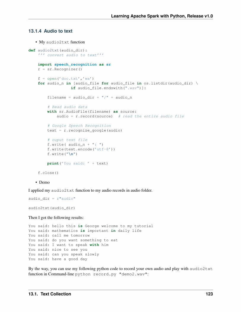
Learning Apache Spark with Python, Release v1.0
13.1.4 Audio to text
• My audio2txt function
def audio2txt(audio_dir):’’’ convert audio to text’’’
import speech_recognition as srr = sr.Recognizer()
f = open(’doc.txt’,’wa’)for audio_n in [audio_file for audio_file in os.listdir(audio_dir) \
if audio_file.endswith(".wav")]:
filename = audio_dir + "/" + audio_n
# Read audio datawith sr.AudioFile(filename) as source:
audio = r.record(source) # read the entire audio file
# Google Speech Recognitiontext = r.recognize_google(audio)
# ouput text filef.write( audio_n + ": ")f.write(text.encode(’utf-8’))f.write("\n")
print(’You said: ’ + text)
f.close()
• Demo
I applied my audio2txt function to my audio records in audio folder.
audio_dir = r"audio"
audio2txt(audio_dir)
Then I got the following results:
You said: hello this is George welcome to my tutorialYou said: mathematics is important in daily lifeYou said: call me tomorrowYou said: do you want something to eatYou said: I want to speak with himYou said: nice to see youYou said: can you speak slowlyYou said: have a good day
By the way, you can use my following python code to record your own audio and play with audio2txtfunction in Command-line python record.py "demo2.wav":
13.1. Text Collection 123
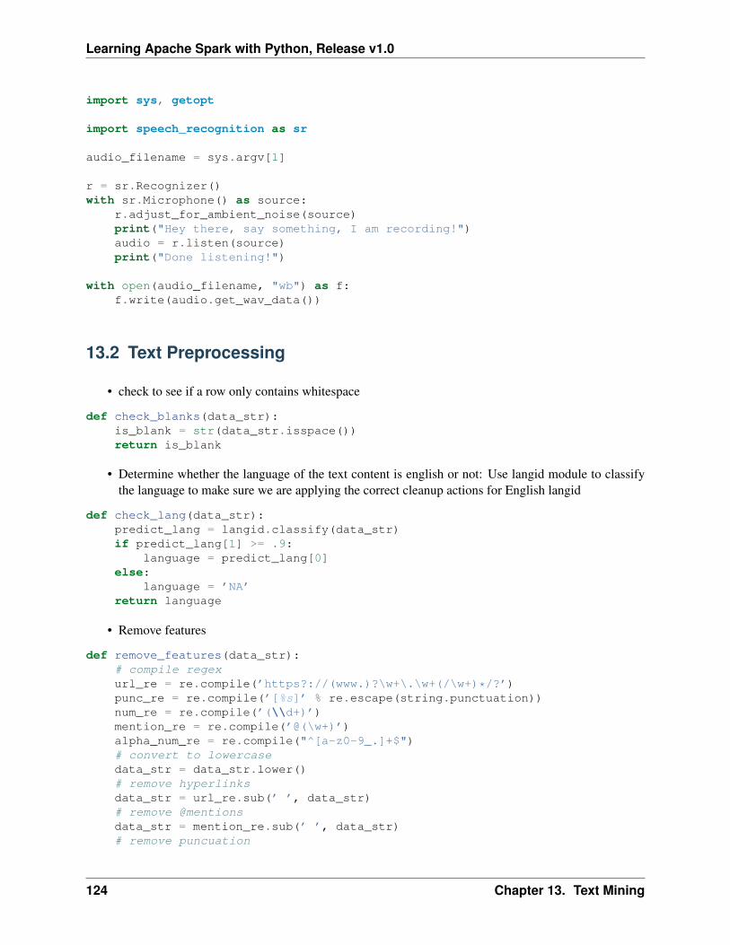
Learning Apache Spark with Python, Release v1.0
import sys, getopt
import speech_recognition as sr
audio_filename = sys.argv[1]
r = sr.Recognizer()with sr.Microphone() as source:
r.adjust_for_ambient_noise(source)print("Hey there, say something, I am recording!")audio = r.listen(source)print("Done listening!")
with open(audio_filename, "wb") as f:f.write(audio.get_wav_data())
13.2 Text Preprocessing
• check to see if a row only contains whitespace
def check_blanks(data_str):is_blank = str(data_str.isspace())return is_blank
• Determine whether the language of the text content is english or not: Use langid module to classifythe language to make sure we are applying the correct cleanup actions for English langid
def check_lang(data_str):predict_lang = langid.classify(data_str)if predict_lang[1] >= .9:
language = predict_lang[0]else:
language = ’NA’return language
• Remove features
def remove_features(data_str):# compile regexurl_re = re.compile(’https?://(www.)?\w+\.\w+(/\w+)*/?’)punc_re = re.compile(’[%s]’ % re.escape(string.punctuation))num_re = re.compile(’(\\d+)’)mention_re = re.compile(’@(\w+)’)alpha_num_re = re.compile("^[a-z0-9_.]+$")# convert to lowercasedata_str = data_str.lower()# remove hyperlinksdata_str = url_re.sub(’ ’, data_str)# remove @mentionsdata_str = mention_re.sub(’ ’, data_str)# remove puncuation
124 Chapter 13. Text Mining
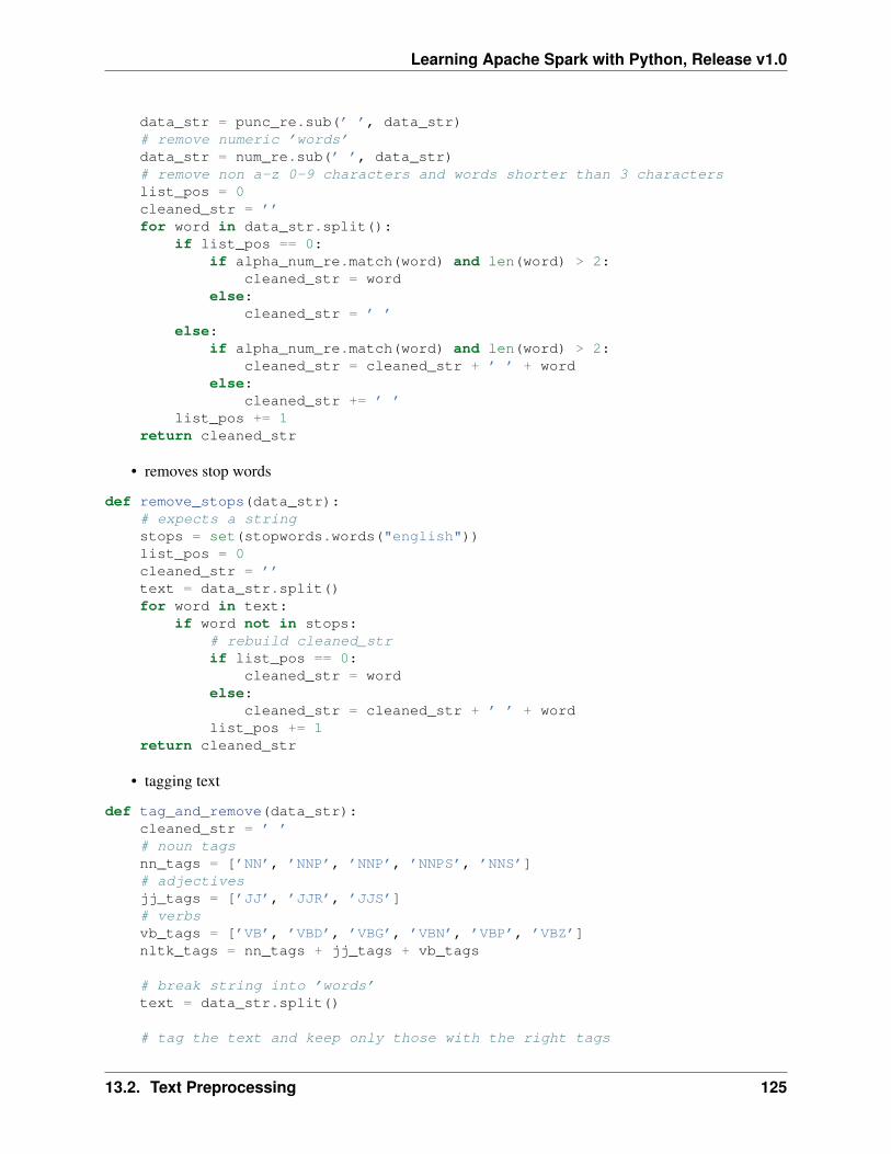
Learning Apache Spark with Python, Release v1.0
data_str = punc_re.sub(’ ’, data_str)# remove numeric ’words’data_str = num_re.sub(’ ’, data_str)# remove non a-z 0-9 characters and words shorter than 3 characterslist_pos = 0cleaned_str = ’’for word in data_str.split():
if list_pos == 0:if alpha_num_re.match(word) and len(word) > 2:
cleaned_str = wordelse:
cleaned_str = ’ ’else:
if alpha_num_re.match(word) and len(word) > 2:cleaned_str = cleaned_str + ’ ’ + word
else:cleaned_str += ’ ’
list_pos += 1return cleaned_str
• removes stop words
def remove_stops(data_str):# expects a stringstops = set(stopwords.words("english"))list_pos = 0cleaned_str = ’’text = data_str.split()for word in text:
if word not in stops:# rebuild cleaned_strif list_pos == 0:
cleaned_str = wordelse:
cleaned_str = cleaned_str + ’ ’ + wordlist_pos += 1
return cleaned_str
• tagging text
def tag_and_remove(data_str):cleaned_str = ’ ’# noun tagsnn_tags = [’NN’, ’NNP’, ’NNP’, ’NNPS’, ’NNS’]# adjectivesjj_tags = [’JJ’, ’JJR’, ’JJS’]# verbsvb_tags = [’VB’, ’VBD’, ’VBG’, ’VBN’, ’VBP’, ’VBZ’]nltk_tags = nn_tags + jj_tags + vb_tags
# break string into ’words’text = data_str.split()
# tag the text and keep only those with the right tags
13.2. Text Preprocessing 125
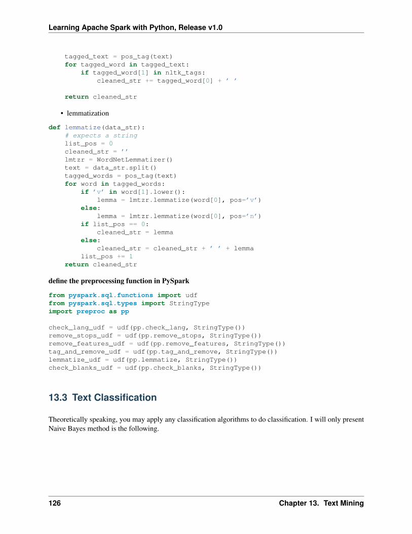
Learning Apache Spark with Python, Release v1.0
tagged_text = pos_tag(text)for tagged_word in tagged_text:
if tagged_word[1] in nltk_tags:cleaned_str += tagged_word[0] + ’ ’
return cleaned_str
• lemmatization
def lemmatize(data_str):# expects a stringlist_pos = 0cleaned_str = ’’lmtzr = WordNetLemmatizer()text = data_str.split()tagged_words = pos_tag(text)for word in tagged_words:
if ’v’ in word[1].lower():lemma = lmtzr.lemmatize(word[0], pos=’v’)
else:lemma = lmtzr.lemmatize(word[0], pos=’n’)
if list_pos == 0:cleaned_str = lemma
else:cleaned_str = cleaned_str + ’ ’ + lemma
list_pos += 1return cleaned_str
define the preprocessing function in PySpark
from pyspark.sql.functions import udffrom pyspark.sql.types import StringTypeimport preproc as pp
check_lang_udf = udf(pp.check_lang, StringType())remove_stops_udf = udf(pp.remove_stops, StringType())remove_features_udf = udf(pp.remove_features, StringType())tag_and_remove_udf = udf(pp.tag_and_remove, StringType())lemmatize_udf = udf(pp.lemmatize, StringType())check_blanks_udf = udf(pp.check_blanks, StringType())
13.3 Text Classification
Theoretically speaking, you may apply any classification algorithms to do classification. I will only presentNaive Bayes method is the following.
126 Chapter 13. Text Mining
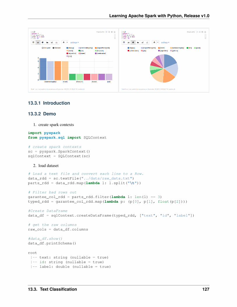
Learning Apache Spark with Python, Release v1.0
13.3.1 Introduction
13.3.2 Demo
1. create spark contexts
import pysparkfrom pyspark.sql import SQLContext
# create spark contextssc = pyspark.SparkContext()sqlContext = SQLContext(sc)
2. load dataset
# Load a text file and convert each line to a Row.data_rdd = sc.textFile("../data/raw_data.txt")parts_rdd = data_rdd.map(lambda l: l.split("\t"))
# Filter bad rows outgarantee_col_rdd = parts_rdd.filter(lambda l: len(l) == 3)typed_rdd = garantee_col_rdd.map(lambda p: (p[0], p[1], float(p[2])))
#Create DataFramedata_df = sqlContext.createDataFrame(typed_rdd, ["text", "id", "label"])
# get the raw columnsraw_cols = data_df.columns
#data_df.show()data_df.printSchema()
root|-- text: string (nullable = true)|-- id: string (nullable = true)|-- label: double (nullable = true)
13.3. Text Classification 127
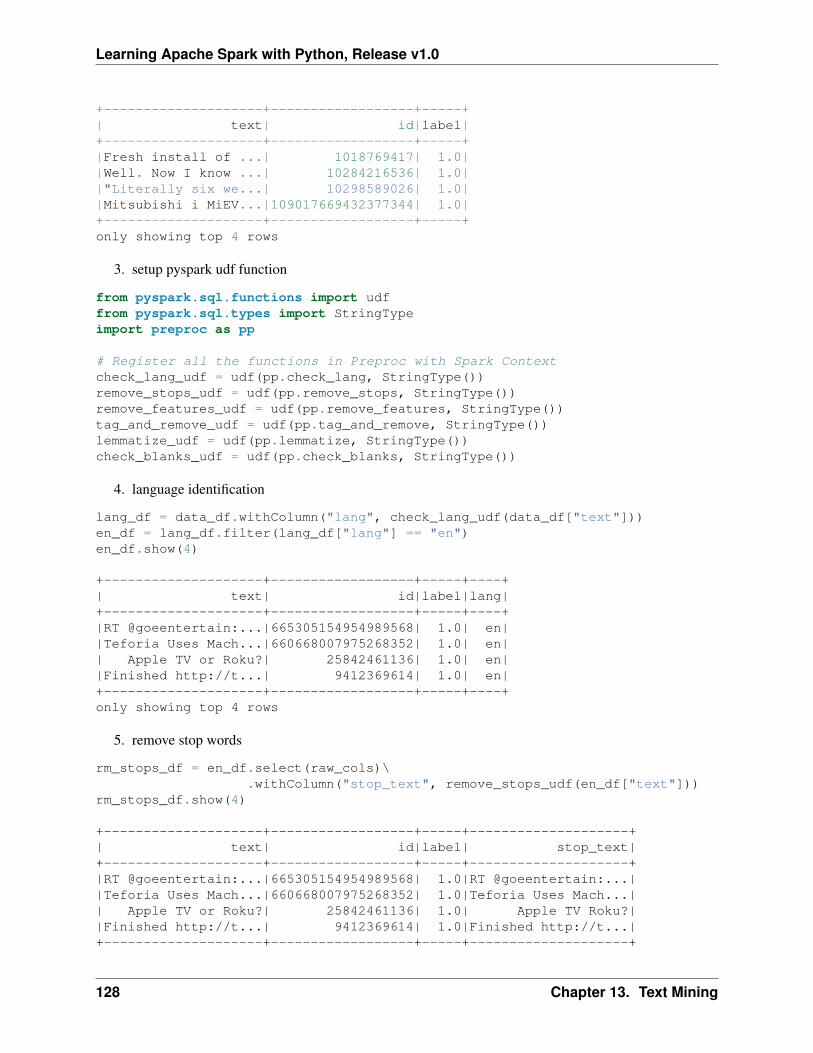
Learning Apache Spark with Python, Release v1.0
+--------------------+------------------+-----+| text| id|label|+--------------------+------------------+-----+|Fresh install of ...| 1018769417| 1.0||Well. Now I know ...| 10284216536| 1.0||"Literally six we...| 10298589026| 1.0||Mitsubishi i MiEV...|109017669432377344| 1.0|+--------------------+------------------+-----+only showing top 4 rows
3. setup pyspark udf function
from pyspark.sql.functions import udffrom pyspark.sql.types import StringTypeimport preproc as pp
# Register all the functions in Preproc with Spark Contextcheck_lang_udf = udf(pp.check_lang, StringType())remove_stops_udf = udf(pp.remove_stops, StringType())remove_features_udf = udf(pp.remove_features, StringType())tag_and_remove_udf = udf(pp.tag_and_remove, StringType())lemmatize_udf = udf(pp.lemmatize, StringType())check_blanks_udf = udf(pp.check_blanks, StringType())
4. language identification
lang_df = data_df.withColumn("lang", check_lang_udf(data_df["text"]))en_df = lang_df.filter(lang_df["lang"] == "en")en_df.show(4)
+--------------------+------------------+-----+----+| text| id|label|lang|+--------------------+------------------+-----+----+|RT @goeentertain:...|665305154954989568| 1.0| en||Teforia Uses Mach...|660668007975268352| 1.0| en|| Apple TV or Roku?| 25842461136| 1.0| en||Finished http://t...| 9412369614| 1.0| en|+--------------------+------------------+-----+----+only showing top 4 rows
5. remove stop words
rm_stops_df = en_df.select(raw_cols)\.withColumn("stop_text", remove_stops_udf(en_df["text"]))
rm_stops_df.show(4)
+--------------------+------------------+-----+--------------------+| text| id|label| stop_text|+--------------------+------------------+-----+--------------------+|RT @goeentertain:...|665305154954989568| 1.0|RT @goeentertain:...||Teforia Uses Mach...|660668007975268352| 1.0|Teforia Uses Mach...|| Apple TV or Roku?| 25842461136| 1.0| Apple TV Roku?||Finished http://t...| 9412369614| 1.0|Finished http://t...|+--------------------+------------------+-----+--------------------+
128 Chapter 13. Text Mining
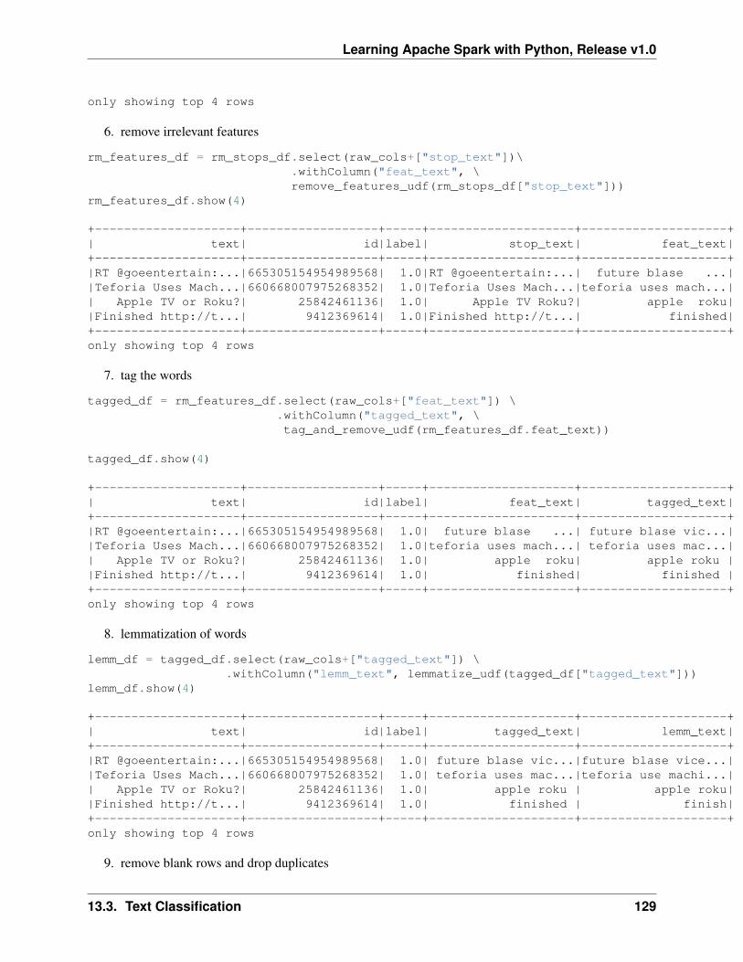
Learning Apache Spark with Python, Release v1.0
only showing top 4 rows
6. remove irrelevant features
rm_features_df = rm_stops_df.select(raw_cols+["stop_text"])\.withColumn("feat_text", \remove_features_udf(rm_stops_df["stop_text"]))
rm_features_df.show(4)
+--------------------+------------------+-----+--------------------+--------------------+| text| id|label| stop_text| feat_text|+--------------------+------------------+-----+--------------------+--------------------+|RT @goeentertain:...|665305154954989568| 1.0|RT @goeentertain:...| future blase ...||Teforia Uses Mach...|660668007975268352| 1.0|Teforia Uses Mach...|teforia uses mach...|| Apple TV or Roku?| 25842461136| 1.0| Apple TV Roku?| apple roku||Finished http://t...| 9412369614| 1.0|Finished http://t...| finished|+--------------------+------------------+-----+--------------------+--------------------+only showing top 4 rows
7. tag the words
tagged_df = rm_features_df.select(raw_cols+["feat_text"]) \.withColumn("tagged_text", \tag_and_remove_udf(rm_features_df.feat_text))
tagged_df.show(4)
+--------------------+------------------+-----+--------------------+--------------------+| text| id|label| feat_text| tagged_text|+--------------------+------------------+-----+--------------------+--------------------+|RT @goeentertain:...|665305154954989568| 1.0| future blase ...| future blase vic...||Teforia Uses Mach...|660668007975268352| 1.0|teforia uses mach...| teforia uses mac...|| Apple TV or Roku?| 25842461136| 1.0| apple roku| apple roku ||Finished http://t...| 9412369614| 1.0| finished| finished |+--------------------+------------------+-----+--------------------+--------------------+only showing top 4 rows
8. lemmatization of words
lemm_df = tagged_df.select(raw_cols+["tagged_text"]) \.withColumn("lemm_text", lemmatize_udf(tagged_df["tagged_text"]))
lemm_df.show(4)
+--------------------+------------------+-----+--------------------+--------------------+| text| id|label| tagged_text| lemm_text|+--------------------+------------------+-----+--------------------+--------------------+|RT @goeentertain:...|665305154954989568| 1.0| future blase vic...|future blase vice...||Teforia Uses Mach...|660668007975268352| 1.0| teforia uses mac...|teforia use machi...|| Apple TV or Roku?| 25842461136| 1.0| apple roku | apple roku||Finished http://t...| 9412369614| 1.0| finished | finish|+--------------------+------------------+-----+--------------------+--------------------+only showing top 4 rows
9. remove blank rows and drop duplicates
13.3. Text Classification 129
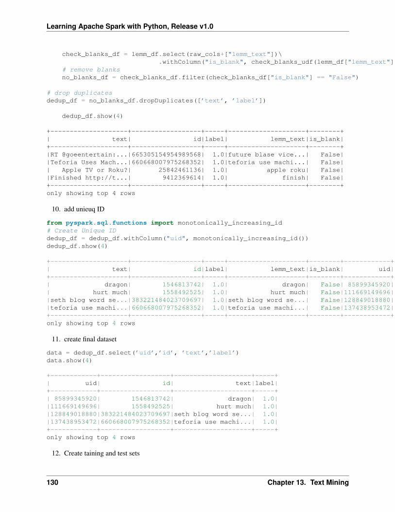
Learning Apache Spark with Python, Release v1.0
check_blanks_df = lemm_df.select(raw_cols+["lemm_text"])\.withColumn("is_blank", check_blanks_udf(lemm_df["lemm_text"]))
# remove blanksno_blanks_df = check_blanks_df.filter(check_blanks_df["is_blank"] == "False")
# drop duplicatesdedup_df = no_blanks_df.dropDuplicates([’text’, ’label’])
dedup_df.show(4)
+--------------------+------------------+-----+--------------------+--------+| text| id|label| lemm_text|is_blank|+--------------------+------------------+-----+--------------------+--------+|RT @goeentertain:...|665305154954989568| 1.0|future blase vice...| False||Teforia Uses Mach...|660668007975268352| 1.0|teforia use machi...| False|| Apple TV or Roku?| 25842461136| 1.0| apple roku| False||Finished http://t...| 9412369614| 1.0| finish| False|+--------------------+------------------+-----+--------------------+--------+only showing top 4 rows
10. add unieuq ID
from pyspark.sql.functions import monotonically_increasing_id# Create Unique IDdedup_df = dedup_df.withColumn("uid", monotonically_increasing_id())dedup_df.show(4)
+--------------------+------------------+-----+--------------------+--------+------------+| text| id|label| lemm_text|is_blank| uid|+--------------------+------------------+-----+--------------------+--------+------------+| dragon| 1546813742| 1.0| dragon| False| 85899345920|| hurt much| 1558492525| 1.0| hurt much| False|111669149696||seth blog word se...|383221484023709697| 1.0|seth blog word se...| False|128849018880||teforia use machi...|660668007975268352| 1.0|teforia use machi...| False|137438953472|+--------------------+------------------+-----+--------------------+--------+------------+only showing top 4 rows
11. create final dataset
data = dedup_df.select(’uid’,’id’, ’text’,’label’)data.show(4)
+------------+------------------+--------------------+-----+| uid| id| text|label|+------------+------------------+--------------------+-----+| 85899345920| 1546813742| dragon| 1.0||111669149696| 1558492525| hurt much| 1.0||128849018880|383221484023709697|seth blog word se...| 1.0||137438953472|660668007975268352|teforia use machi...| 1.0|+------------+------------------+--------------------+-----+only showing top 4 rows
12. Create taining and test sets
130 Chapter 13. Text Mining
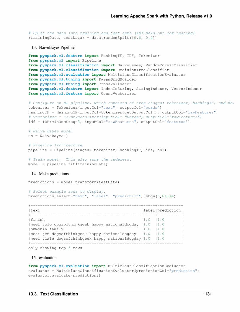
Learning Apache Spark with Python, Release v1.0
# Split the data into training and test sets (40% held out for testing)(trainingData, testData) = data.randomSplit([0.6, 0.4])
13. NaiveBayes Pipeline
from pyspark.ml.feature import HashingTF, IDF, Tokenizerfrom pyspark.ml import Pipelinefrom pyspark.ml.classification import NaiveBayes, RandomForestClassifierfrom pyspark.ml.classification import DecisionTreeClassifierfrom pyspark.ml.evaluation import MulticlassClassificationEvaluatorfrom pyspark.ml.tuning import ParamGridBuilderfrom pyspark.ml.tuning import CrossValidatorfrom pyspark.ml.feature import IndexToString, StringIndexer, VectorIndexerfrom pyspark.ml.feature import CountVectorizer
# Configure an ML pipeline, which consists of tree stages: tokenizer, hashingTF, and nb.tokenizer = Tokenizer(inputCol="text", outputCol="words")hashingTF = HashingTF(inputCol=tokenizer.getOutputCol(), outputCol="rawFeatures")# vectorizer = CountVectorizer(inputCol= "words", outputCol="rawFeatures")idf = IDF(minDocFreq=3, inputCol="rawFeatures", outputCol="features")
# Naive Bayes modelnb = NaiveBayes()
# Pipeline Architecturepipeline = Pipeline(stages=[tokenizer, hashingTF, idf, nb])
# Train model. This also runs the indexers.model = pipeline.fit(trainingData)
14. Make predictions
predictions = model.transform(testData)
# Select example rows to display.predictions.select("text", "label", "prediction").show(5,False)
+-----------------------------------------------+-----+----------+|text |label|prediction|+-----------------------------------------------+-----+----------+|finish |1.0 |1.0 ||meet rolo dogsofthinkgeek happy nationaldogday |1.0 |1.0 ||pumpkin family |1.0 |1.0 ||meet jet dogsofthinkgeek happy nationaldogday |1.0 |1.0 ||meet vixie dogsofthinkgeek happy nationaldogday|1.0 |1.0 |+-----------------------------------------------+-----+----------+only showing top 5 rows
15. evaluation
from pyspark.ml.evaluation import MulticlassClassificationEvaluatorevaluator = MulticlassClassificationEvaluator(predictionCol="prediction")evaluator.evaluate(predictions)
13.3. Text Classification 131
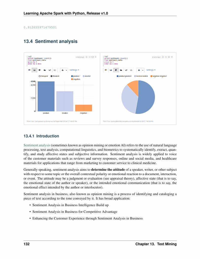
Learning Apache Spark with Python, Release v1.0
0.912655971479501
13.4 Sentiment analysis
13.4.1 Introduction
Sentiment analysis (sometimes known as opinion mining or emotion AI) refers to the use of natural languageprocessing, text analysis, computational linguistics, and biometrics to systematically identify, extract, quan-tify, and study affective states and subjective information. Sentiment analysis is widely applied to voiceof the customer materials such as reviews and survey responses, online and social media, and healthcarematerials for applications that range from marketing to customer service to clinical medicine.
Generally speaking, sentiment analysis aims to determine the attitude of a speaker, writer, or other subjectwith respect to some topic or the overall contextual polarity or emotional reaction to a document, interaction,or event. The attitude may be a judgment or evaluation (see appraisal theory), affective state (that is to say,the emotional state of the author or speaker), or the intended emotional communication (that is to say, theemotional effect intended by the author or interlocutor).
Sentiment analysis in business, also known as opinion mining is a process of identifying and cataloging apiece of text according to the tone conveyed by it. It has broad application:
• Sentiment Analysis in Business Intelligence Build up
• Sentiment Analysis in Business for Competitive Advantage
• Enhancing the Customer Experience through Sentiment Analysis in Business
132 Chapter 13. Text Mining
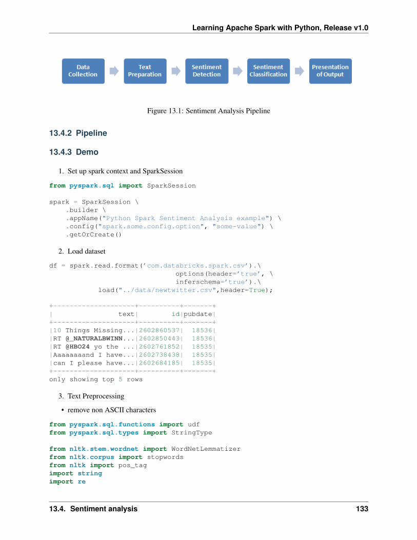
Learning Apache Spark with Python, Release v1.0
Figure 13.1: Sentiment Analysis Pipeline
13.4.2 Pipeline
13.4.3 Demo
1. Set up spark context and SparkSession
from pyspark.sql import SparkSession
spark = SparkSession \.builder \.appName("Python Spark Sentiment Analysis example") \.config("spark.some.config.option", "some-value") \.getOrCreate()
2. Load dataset
df = spark.read.format(’com.databricks.spark.csv’).\options(header=’true’, \inferschema=’true’).\
load("../data/newtwitter.csv",header=True);
+--------------------+----------+-------+| text| id|pubdate|+--------------------+----------+-------+|10 Things Missing...|2602860537| 18536||RT @_NATURALBWINN...|2602850443| 18536||RT @HBO24 yo the ...|2602761852| 18535||Aaaaaaaand I have...|2602738438| 18535||can I please have...|2602684185| 18535|+--------------------+----------+-------+only showing top 5 rows
3. Text Preprocessing
• remove non ASCII characters
from pyspark.sql.functions import udffrom pyspark.sql.types import StringType
from nltk.stem.wordnet import WordNetLemmatizerfrom nltk.corpus import stopwordsfrom nltk import pos_tagimport stringimport re
13.4. Sentiment analysis 133
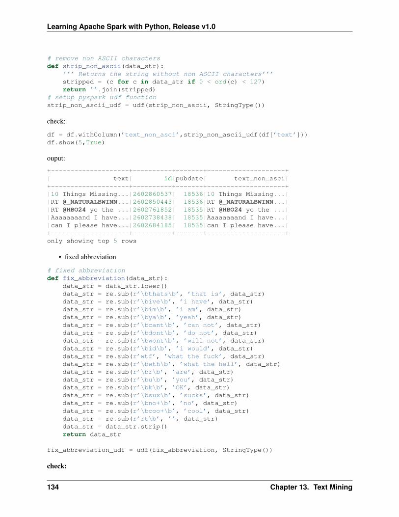
Learning Apache Spark with Python, Release v1.0
# remove non ASCII charactersdef strip_non_ascii(data_str):
’’’ Returns the string without non ASCII characters’’’stripped = (c for c in data_str if 0 < ord(c) < 127)return ’’.join(stripped)
# setup pyspark udf functionstrip_non_ascii_udf = udf(strip_non_ascii, StringType())
check:
df = df.withColumn(’text_non_asci’,strip_non_ascii_udf(df[’text’]))df.show(5,True)
ouput:
+--------------------+----------+-------+--------------------+| text| id|pubdate| text_non_asci|+--------------------+----------+-------+--------------------+|10 Things Missing...|2602860537| 18536|10 Things Missing...||RT @_NATURALBWINN...|2602850443| 18536|RT @_NATURALBWINN...||RT @HBO24 yo the ...|2602761852| 18535|RT @HBO24 yo the ...||Aaaaaaaand I have...|2602738438| 18535|Aaaaaaaand I have...||can I please have...|2602684185| 18535|can I please have...|+--------------------+----------+-------+--------------------+only showing top 5 rows
• fixed abbreviation
# fixed abbreviationdef fix_abbreviation(data_str):
data_str = data_str.lower()data_str = re.sub(r’\bthats\b’, ’that is’, data_str)data_str = re.sub(r’\bive\b’, ’i have’, data_str)data_str = re.sub(r’\bim\b’, ’i am’, data_str)data_str = re.sub(r’\bya\b’, ’yeah’, data_str)data_str = re.sub(r’\bcant\b’, ’can not’, data_str)data_str = re.sub(r’\bdont\b’, ’do not’, data_str)data_str = re.sub(r’\bwont\b’, ’will not’, data_str)data_str = re.sub(r’\bid\b’, ’i would’, data_str)data_str = re.sub(r’wtf’, ’what the fuck’, data_str)data_str = re.sub(r’\bwth\b’, ’what the hell’, data_str)data_str = re.sub(r’\br\b’, ’are’, data_str)data_str = re.sub(r’\bu\b’, ’you’, data_str)data_str = re.sub(r’\bk\b’, ’OK’, data_str)data_str = re.sub(r’\bsux\b’, ’sucks’, data_str)data_str = re.sub(r’\bno+\b’, ’no’, data_str)data_str = re.sub(r’\bcoo+\b’, ’cool’, data_str)data_str = re.sub(r’rt\b’, ’’, data_str)data_str = data_str.strip()return data_str
fix_abbreviation_udf = udf(fix_abbreviation, StringType())
check:
134 Chapter 13. Text Mining
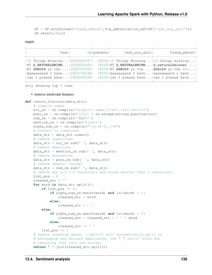
Learning Apache Spark with Python, Release v1.0
df = df.withColumn(’fixed_abbrev’,fix_abbreviation_udf(df[’text_non_asci’]))df.show(5,True)
ouput:
+--------------------+----------+-------+--------------------+--------------------+| text| id|pubdate| text_non_asci| fixed_abbrev|+--------------------+----------+-------+--------------------+--------------------+|10 Things Missing...|2602860537| 18536|10 Things Missing...|10 things missing...||RT @_NATURALBWINN...|2602850443| 18536|RT @_NATURALBWINN...|@_naturalbwinner ...||RT @HBO24 yo the ...|2602761852| 18535|RT @HBO24 yo the ...|@hbo24 yo the #ne...||Aaaaaaaand I have...|2602738438| 18535|Aaaaaaaand I have...|aaaaaaaand i have...||can I please have...|2602684185| 18535|can I please have...|can i please have...|+--------------------+----------+-------+--------------------+--------------------+only showing top 5 rows
• remove irrelevant features
def remove_features(data_str):# compile regexurl_re = re.compile(’https?://(www.)?\w+\.\w+(/\w+)*/?’)punc_re = re.compile(’[%s]’ % re.escape(string.punctuation))num_re = re.compile(’(\\d+)’)mention_re = re.compile(’@(\w+)’)alpha_num_re = re.compile("^[a-z0-9_.]+$")# convert to lowercasedata_str = data_str.lower()# remove hyperlinksdata_str = url_re.sub(’ ’, data_str)# remove @mentionsdata_str = mention_re.sub(’ ’, data_str)# remove puncuationdata_str = punc_re.sub(’ ’, data_str)# remove numeric ’words’data_str = num_re.sub(’ ’, data_str)# remove non a-z 0-9 characters and words shorter than 1 characterslist_pos = 0cleaned_str = ’’for word in data_str.split():
if list_pos == 0:if alpha_num_re.match(word) and len(word) > 1:
cleaned_str = wordelse:
cleaned_str = ’ ’else:
if alpha_num_re.match(word) and len(word) > 1:cleaned_str = cleaned_str + ’ ’ + word
else:cleaned_str += ’ ’
list_pos += 1# remove unwanted space, *.split() will automatically split on# whitespace and discard duplicates, the " ".join() joins the# resulting list into one string.return " ".join(cleaned_str.split())
13.4. Sentiment analysis 135
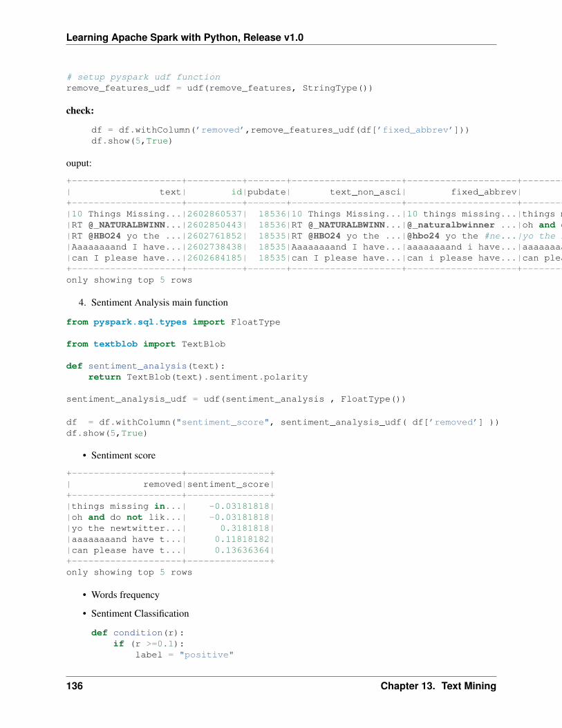
Learning Apache Spark with Python, Release v1.0
# setup pyspark udf functionremove_features_udf = udf(remove_features, StringType())
check:
df = df.withColumn(’removed’,remove_features_udf(df[’fixed_abbrev’]))df.show(5,True)
ouput:
+--------------------+----------+-------+--------------------+--------------------+--------------------+| text| id|pubdate| text_non_asci| fixed_abbrev| removed|+--------------------+----------+-------+--------------------+--------------------+--------------------+|10 Things Missing...|2602860537| 18536|10 Things Missing...|10 things missing...|things missing in...||RT @_NATURALBWINN...|2602850443| 18536|RT @_NATURALBWINN...|@_naturalbwinner ...|oh and do not lik...||RT @HBO24 yo the ...|2602761852| 18535|RT @HBO24 yo the ...|@hbo24 yo the #ne...|yo the newtwitter...||Aaaaaaaand I have...|2602738438| 18535|Aaaaaaaand I have...|aaaaaaaand i have...|aaaaaaaand have t...||can I please have...|2602684185| 18535|can I please have...|can i please have...|can please have t...|+--------------------+----------+-------+--------------------+--------------------+--------------------+only showing top 5 rows
4. Sentiment Analysis main function
from pyspark.sql.types import FloatType
from textblob import TextBlob
def sentiment_analysis(text):return TextBlob(text).sentiment.polarity
sentiment_analysis_udf = udf(sentiment_analysis , FloatType())
df = df.withColumn("sentiment_score", sentiment_analysis_udf( df[’removed’] ))df.show(5,True)
• Sentiment score
+--------------------+---------------+| removed|sentiment_score|+--------------------+---------------+|things missing in...| -0.03181818||oh and do not lik...| -0.03181818||yo the newtwitter...| 0.3181818||aaaaaaaand have t...| 0.11818182||can please have t...| 0.13636364|+--------------------+---------------+only showing top 5 rows
• Words frequency
• Sentiment Classification
def condition(r):if (r >=0.1):
label = "positive"
136 Chapter 13. Text Mining
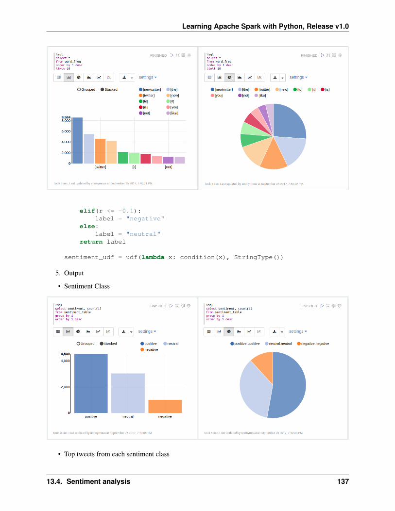
Learning Apache Spark with Python, Release v1.0
elif(r <= -0.1):label = "negative"
else:label = "neutral"
return label
sentiment_udf = udf(lambda x: condition(x), StringType())
5. Output
• Sentiment Class
• Top tweets from each sentiment class
13.4. Sentiment analysis 137
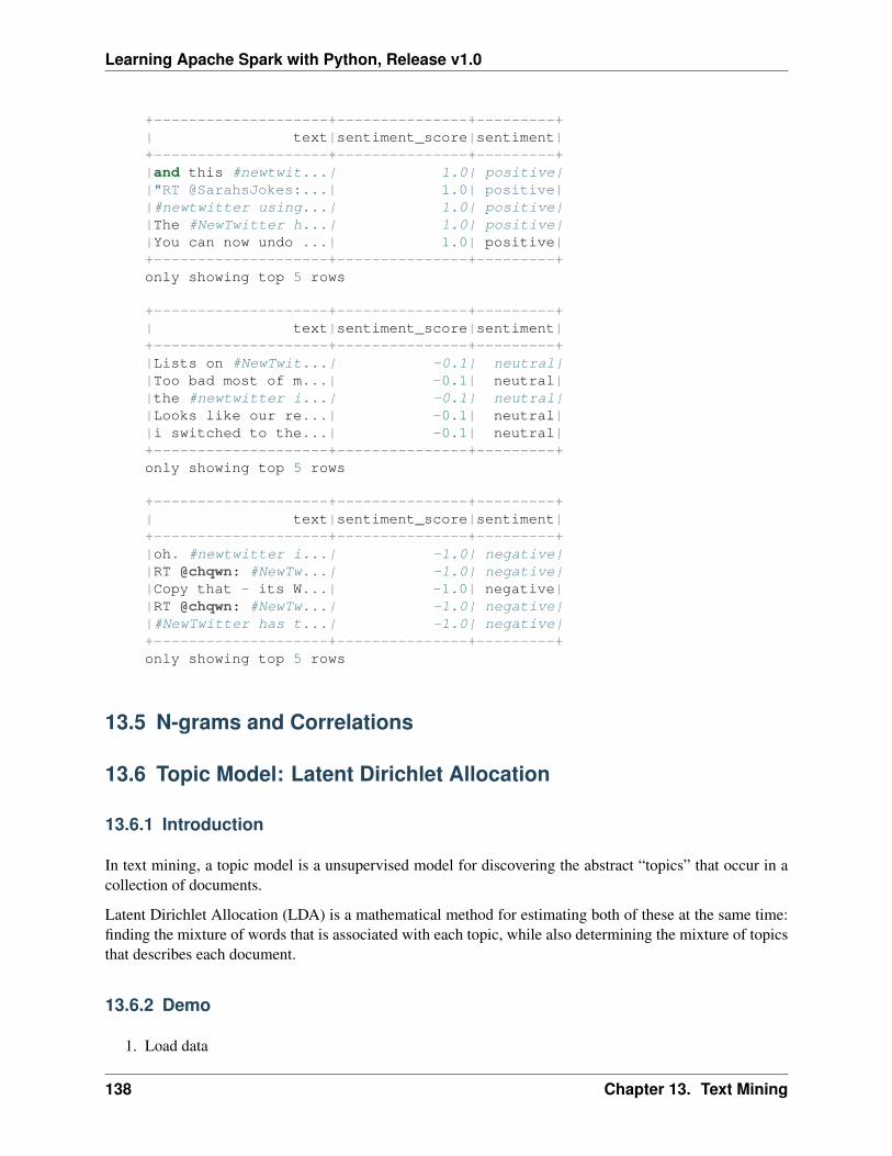
Learning Apache Spark with Python, Release v1.0
+--------------------+---------------+---------+| text|sentiment_score|sentiment|+--------------------+---------------+---------+|and this #newtwit...| 1.0| positive||"RT @SarahsJokes:...| 1.0| positive||#newtwitter using...| 1.0| positive||The #NewTwitter h...| 1.0| positive||You can now undo ...| 1.0| positive|+--------------------+---------------+---------+only showing top 5 rows
+--------------------+---------------+---------+| text|sentiment_score|sentiment|+--------------------+---------------+---------+|Lists on #NewTwit...| -0.1| neutral||Too bad most of m...| -0.1| neutral||the #newtwitter i...| -0.1| neutral||Looks like our re...| -0.1| neutral||i switched to the...| -0.1| neutral|+--------------------+---------------+---------+only showing top 5 rows
+--------------------+---------------+---------+| text|sentiment_score|sentiment|+--------------------+---------------+---------+|oh. #newtwitter i...| -1.0| negative||RT @chqwn: #NewTw...| -1.0| negative||Copy that - its W...| -1.0| negative||RT @chqwn: #NewTw...| -1.0| negative||#NewTwitter has t...| -1.0| negative|+--------------------+---------------+---------+only showing top 5 rows
13.5 N-grams and Correlations
13.6 Topic Model: Latent Dirichlet Allocation
13.6.1 Introduction
In text mining, a topic model is a unsupervised model for discovering the abstract “topics” that occur in acollection of documents.
Latent Dirichlet Allocation (LDA) is a mathematical method for estimating both of these at the same time:finding the mixture of words that is associated with each topic, while also determining the mixture of topicsthat describes each document.
13.6.2 Demo
1. Load data
138 Chapter 13. Text Mining

Learning Apache Spark with Python, Release v1.0
rawdata = spark.read.load("../data/airlines.csv", format="csv", header=True)rawdata.show(5)
+-----+---------------+---------+--------+------+--------+-----+-----------+--------------------+| id| airline| date|location|rating| cabin|value|recommended| review|+-----+---------------+---------+--------+------+--------+-----+-----------+--------------------+|10001|Delta Air Lines|21-Jun-14|Thailand| 7| Economy| 4| YES|Flew Mar 30 NRT t...||10002|Delta Air Lines|19-Jun-14| USA| 0| Economy| 2| NO|Flight 2463 leavi...||10003|Delta Air Lines|18-Jun-14| USA| 0| Economy| 1| NO|Delta Website fro...||10004|Delta Air Lines|17-Jun-14| USA| 9|Business| 4| YES|"I just returned ...||10005|Delta Air Lines|17-Jun-14| Ecuador| 7| Economy| 3| YES|"Round-trip fligh...|+-----+---------------+---------+--------+------+--------+-----+-----------+--------------------+only showing top 5 rows
1. Text preprocessing
I will use the following raw column names to keep my table concise:
raw_cols = rawdata.columnsraw_cols
[’id’, ’airline’, ’date’, ’location’, ’rating’, ’cabin’, ’value’, ’recommended’, ’review’]
rawdata = rawdata.dropDuplicates([’review’])
from pyspark.sql.functions import udf, colfrom pyspark.sql.types import StringType, DoubleType, DateType
from nltk.stem.wordnet import WordNetLemmatizerfrom nltk.corpus import stopwordsfrom nltk import pos_tagimport langidimport stringimport re
• remove non ASCII characters
13.6. Topic Model: Latent Dirichlet Allocation 139
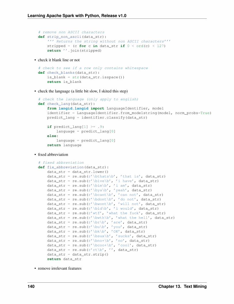
Learning Apache Spark with Python, Release v1.0
# remove non ASCII charactersdef strip_non_ascii(data_str):
’’’ Returns the string without non ASCII characters’’’stripped = (c for c in data_str if 0 < ord(c) < 127)return ’’.join(stripped)
• check it blank line or not
# check to see if a row only contains whitespacedef check_blanks(data_str):
is_blank = str(data_str.isspace())return is_blank
• check the language (a little bit slow, I skited this step)
# check the language (only apply to english)def check_lang(data_str):
from langid.langid import LanguageIdentifier, modelidentifier = LanguageIdentifier.from_modelstring(model, norm_probs=True)predict_lang = identifier.classify(data_str)
if predict_lang[1] >= .9:language = predict_lang[0]
else:language = predict_lang[0]
return language
• fixed abbreviation
# fixed abbreviationdef fix_abbreviation(data_str):
data_str = data_str.lower()data_str = re.sub(r’\bthats\b’, ’that is’, data_str)data_str = re.sub(r’\bive\b’, ’i have’, data_str)data_str = re.sub(r’\bim\b’, ’i am’, data_str)data_str = re.sub(r’\bya\b’, ’yeah’, data_str)data_str = re.sub(r’\bcant\b’, ’can not’, data_str)data_str = re.sub(r’\bdont\b’, ’do not’, data_str)data_str = re.sub(r’\bwont\b’, ’will not’, data_str)data_str = re.sub(r’\bid\b’, ’i would’, data_str)data_str = re.sub(r’wtf’, ’what the fuck’, data_str)data_str = re.sub(r’\bwth\b’, ’what the hell’, data_str)data_str = re.sub(r’\br\b’, ’are’, data_str)data_str = re.sub(r’\bu\b’, ’you’, data_str)data_str = re.sub(r’\bk\b’, ’OK’, data_str)data_str = re.sub(r’\bsux\b’, ’sucks’, data_str)data_str = re.sub(r’\bno+\b’, ’no’, data_str)data_str = re.sub(r’\bcoo+\b’, ’cool’, data_str)data_str = re.sub(r’rt\b’, ’’, data_str)data_str = data_str.strip()return data_str
• remove irrelevant features
140 Chapter 13. Text Mining
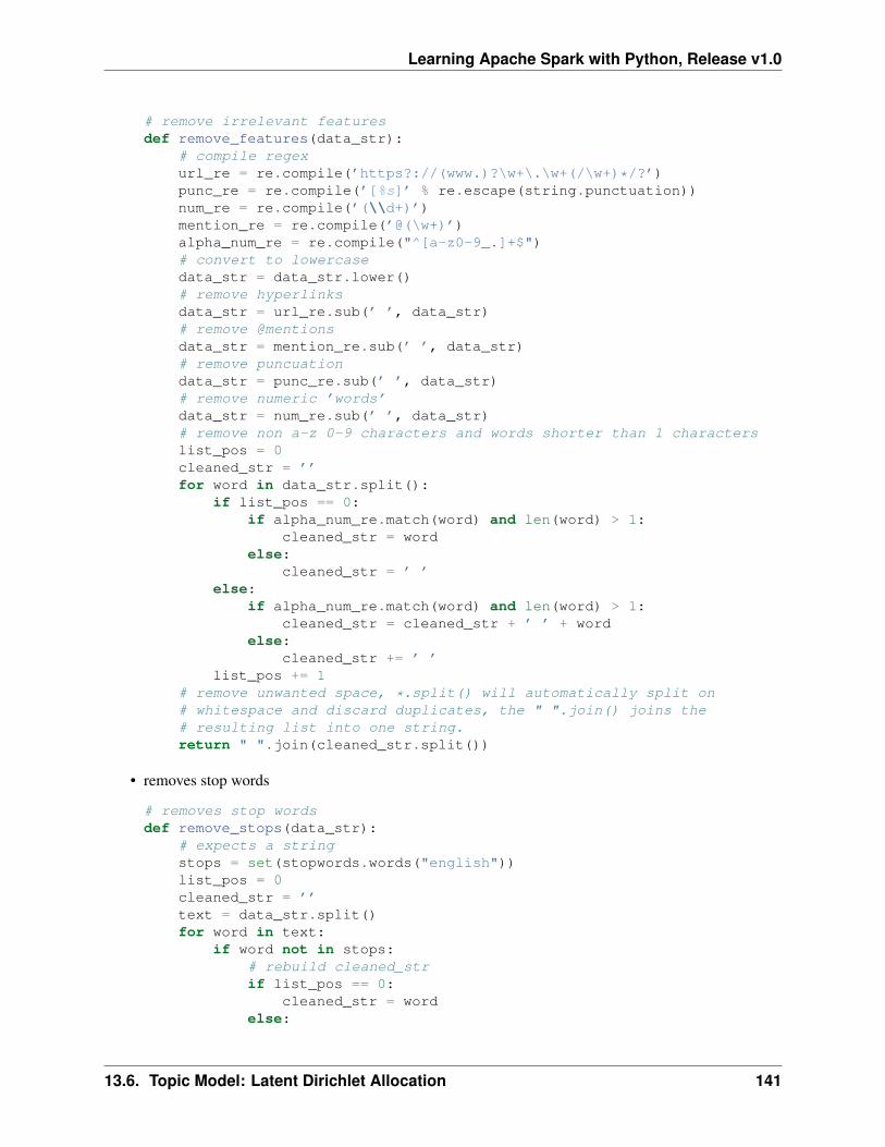
Learning Apache Spark with Python, Release v1.0
# remove irrelevant featuresdef remove_features(data_str):
# compile regexurl_re = re.compile(’https?://(www.)?\w+\.\w+(/\w+)*/?’)punc_re = re.compile(’[%s]’ % re.escape(string.punctuation))num_re = re.compile(’(\\d+)’)mention_re = re.compile(’@(\w+)’)alpha_num_re = re.compile("^[a-z0-9_.]+$")# convert to lowercasedata_str = data_str.lower()# remove hyperlinksdata_str = url_re.sub(’ ’, data_str)# remove @mentionsdata_str = mention_re.sub(’ ’, data_str)# remove puncuationdata_str = punc_re.sub(’ ’, data_str)# remove numeric ’words’data_str = num_re.sub(’ ’, data_str)# remove non a-z 0-9 characters and words shorter than 1 characterslist_pos = 0cleaned_str = ’’for word in data_str.split():
if list_pos == 0:if alpha_num_re.match(word) and len(word) > 1:
cleaned_str = wordelse:
cleaned_str = ’ ’else:
if alpha_num_re.match(word) and len(word) > 1:cleaned_str = cleaned_str + ’ ’ + word
else:cleaned_str += ’ ’
list_pos += 1# remove unwanted space, *.split() will automatically split on# whitespace and discard duplicates, the " ".join() joins the# resulting list into one string.return " ".join(cleaned_str.split())
• removes stop words
# removes stop wordsdef remove_stops(data_str):
# expects a stringstops = set(stopwords.words("english"))list_pos = 0cleaned_str = ’’text = data_str.split()for word in text:
if word not in stops:# rebuild cleaned_strif list_pos == 0:
cleaned_str = wordelse:
13.6. Topic Model: Latent Dirichlet Allocation 141
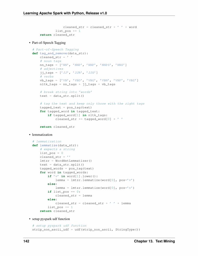
Learning Apache Spark with Python, Release v1.0
cleaned_str = cleaned_str + ’ ’ + wordlist_pos += 1
return cleaned_str
• Part-of-Speech Tagging
# Part-of-Speech Taggingdef tag_and_remove(data_str):
cleaned_str = ’ ’# noun tagsnn_tags = [’NN’, ’NNP’, ’NNP’, ’NNPS’, ’NNS’]# adjectivesjj_tags = [’JJ’, ’JJR’, ’JJS’]# verbsvb_tags = [’VB’, ’VBD’, ’VBG’, ’VBN’, ’VBP’, ’VBZ’]nltk_tags = nn_tags + jj_tags + vb_tags
# break string into ’words’text = data_str.split()
# tag the text and keep only those with the right tagstagged_text = pos_tag(text)for tagged_word in tagged_text:
if tagged_word[1] in nltk_tags:cleaned_str += tagged_word[0] + ’ ’
return cleaned_str
• lemmatization
# lemmatizationdef lemmatize(data_str):
# expects a stringlist_pos = 0cleaned_str = ’’lmtzr = WordNetLemmatizer()text = data_str.split()tagged_words = pos_tag(text)for word in tagged_words:
if ’v’ in word[1].lower():lemma = lmtzr.lemmatize(word[0], pos=’v’)
else:lemma = lmtzr.lemmatize(word[0], pos=’n’)
if list_pos == 0:cleaned_str = lemma
else:cleaned_str = cleaned_str + ’ ’ + lemma
list_pos += 1return cleaned_str
• setup pyspark udf function
# setup pyspark udf functionstrip_non_ascii_udf = udf(strip_non_ascii, StringType())
142 Chapter 13. Text Mining
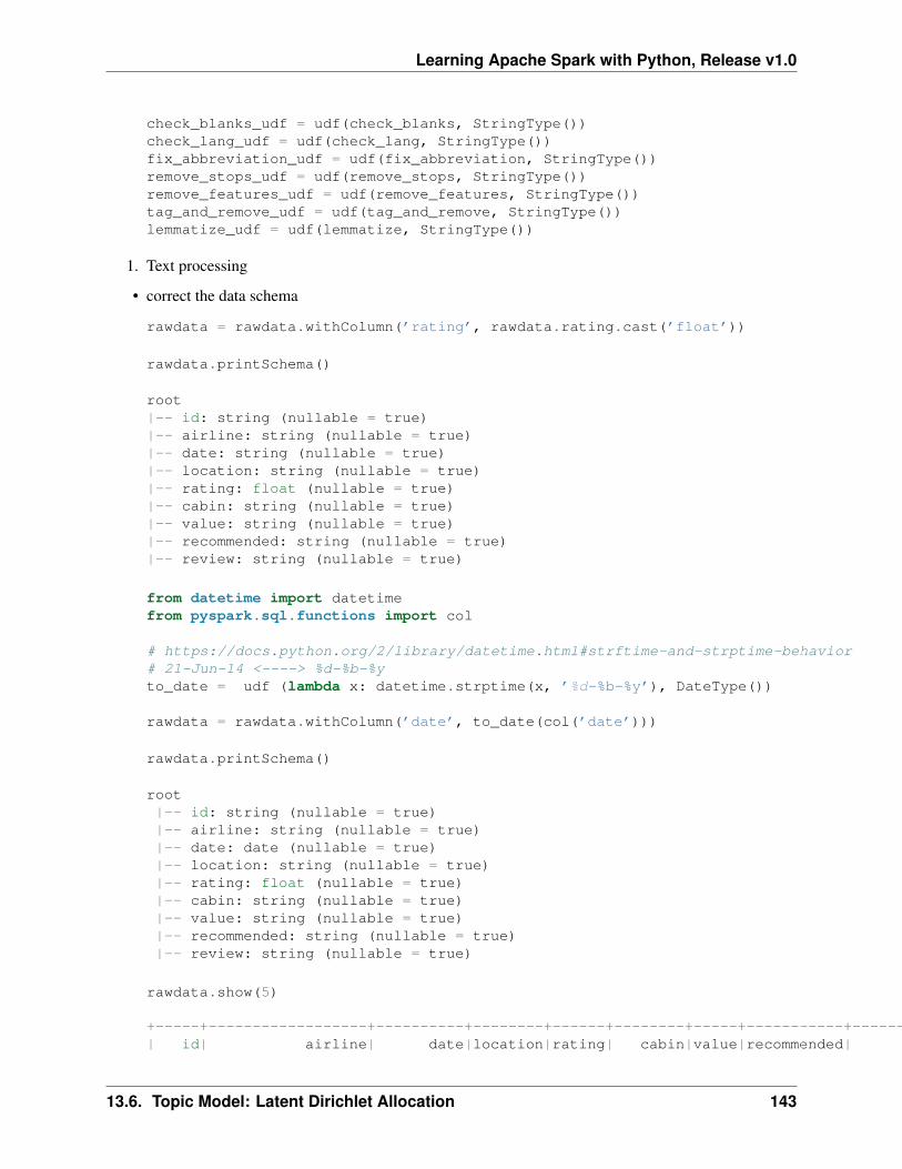
Learning Apache Spark with Python, Release v1.0
check_blanks_udf = udf(check_blanks, StringType())check_lang_udf = udf(check_lang, StringType())fix_abbreviation_udf = udf(fix_abbreviation, StringType())remove_stops_udf = udf(remove_stops, StringType())remove_features_udf = udf(remove_features, StringType())tag_and_remove_udf = udf(tag_and_remove, StringType())lemmatize_udf = udf(lemmatize, StringType())
1. Text processing
• correct the data schema
rawdata = rawdata.withColumn(’rating’, rawdata.rating.cast(’float’))
rawdata.printSchema()
root|-- id: string (nullable = true)|-- airline: string (nullable = true)|-- date: string (nullable = true)|-- location: string (nullable = true)|-- rating: float (nullable = true)|-- cabin: string (nullable = true)|-- value: string (nullable = true)|-- recommended: string (nullable = true)|-- review: string (nullable = true)
from datetime import datetimefrom pyspark.sql.functions import col
# https://docs.python.org/2/library/datetime.html#strftime-and-strptime-behavior# 21-Jun-14 <----> %d-%b-%yto_date = udf (lambda x: datetime.strptime(x, ’%d-%b-%y’), DateType())
rawdata = rawdata.withColumn(’date’, to_date(col(’date’)))
rawdata.printSchema()
root|-- id: string (nullable = true)|-- airline: string (nullable = true)|-- date: date (nullable = true)|-- location: string (nullable = true)|-- rating: float (nullable = true)|-- cabin: string (nullable = true)|-- value: string (nullable = true)|-- recommended: string (nullable = true)|-- review: string (nullable = true)
rawdata.show(5)
+-----+------------------+----------+--------+------+--------+-----+-----------+--------------------+| id| airline| date|location|rating| cabin|value|recommended| review|
13.6. Topic Model: Latent Dirichlet Allocation 143
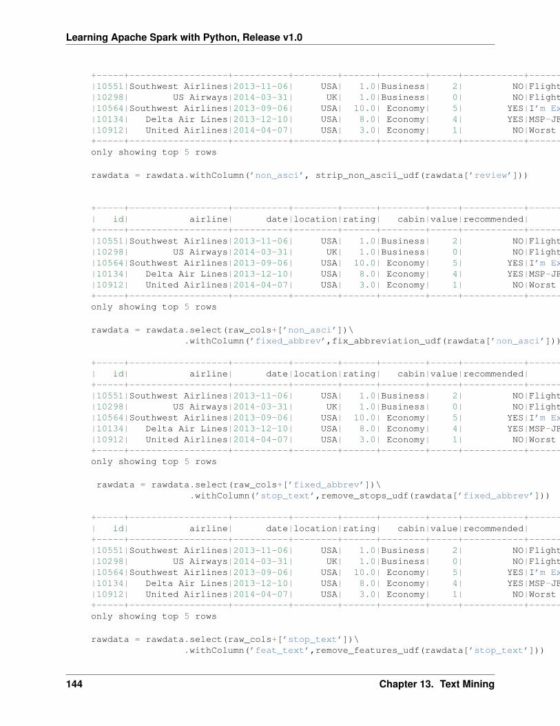
Learning Apache Spark with Python, Release v1.0
+-----+------------------+----------+--------+------+--------+-----+-----------+--------------------+|10551|Southwest Airlines|2013-11-06| USA| 1.0|Business| 2| NO|Flight 3246 from ...||10298| US Airways|2014-03-31| UK| 1.0|Business| 0| NO|Flight from Manch...||10564|Southwest Airlines|2013-09-06| USA| 10.0| Economy| 5| YES|I’m Executive Pla...||10134| Delta Air Lines|2013-12-10| USA| 8.0| Economy| 4| YES|MSP-JFK-MXP and r...||10912| United Airlines|2014-04-07| USA| 3.0| Economy| 1| NO|Worst airline I h...|+-----+------------------+----------+--------+------+--------+-----+-----------+--------------------+only showing top 5 rows
rawdata = rawdata.withColumn(’non_asci’, strip_non_ascii_udf(rawdata[’review’]))
+-----+------------------+----------+--------+------+--------+-----+-----------+--------------------+--------------------+| id| airline| date|location|rating| cabin|value|recommended| review| non_asci|+-----+------------------+----------+--------+------+--------+-----+-----------+--------------------+--------------------+|10551|Southwest Airlines|2013-11-06| USA| 1.0|Business| 2| NO|Flight 3246 from ...|Flight 3246 from ...||10298| US Airways|2014-03-31| UK| 1.0|Business| 0| NO|Flight from Manch...|Flight from Manch...||10564|Southwest Airlines|2013-09-06| USA| 10.0| Economy| 5| YES|I’m Executive Pla...|I’m Executive Pla...||10134| Delta Air Lines|2013-12-10| USA| 8.0| Economy| 4| YES|MSP-JFK-MXP and r...|MSP-JFK-MXP and r...||10912| United Airlines|2014-04-07| USA| 3.0| Economy| 1| NO|Worst airline I h...|Worst airline I h...|+-----+------------------+----------+--------+------+--------+-----+-----------+--------------------+--------------------+only showing top 5 rows
rawdata = rawdata.select(raw_cols+[’non_asci’])\.withColumn(’fixed_abbrev’,fix_abbreviation_udf(rawdata[’non_asci’]))
+-----+------------------+----------+--------+------+--------+-----+-----------+--------------------+--------------------+--------------------+| id| airline| date|location|rating| cabin|value|recommended| review| non_asci| fixed_abbrev|+-----+------------------+----------+--------+------+--------+-----+-----------+--------------------+--------------------+--------------------+|10551|Southwest Airlines|2013-11-06| USA| 1.0|Business| 2| NO|Flight 3246 from ...|Flight 3246 from ...|flight 3246 from ...||10298| US Airways|2014-03-31| UK| 1.0|Business| 0| NO|Flight from Manch...|Flight from Manch...|flight from manch...||10564|Southwest Airlines|2013-09-06| USA| 10.0| Economy| 5| YES|I’m Executive Pla...|I’m Executive Pla...|i’m executive pla...||10134| Delta Air Lines|2013-12-10| USA| 8.0| Economy| 4| YES|MSP-JFK-MXP and r...|MSP-JFK-MXP and r...|msp-jfk-mxp and r...||10912| United Airlines|2014-04-07| USA| 3.0| Economy| 1| NO|Worst airline I h...|Worst airline I h...|worst airline i h...|+-----+------------------+----------+--------+------+--------+-----+-----------+--------------------+--------------------+--------------------+only showing top 5 rows
rawdata = rawdata.select(raw_cols+[’fixed_abbrev’])\.withColumn(’stop_text’,remove_stops_udf(rawdata[’fixed_abbrev’]))
+-----+------------------+----------+--------+------+--------+-----+-----------+--------------------+--------------------+--------------------+| id| airline| date|location|rating| cabin|value|recommended| review| fixed_abbrev| stop_text|+-----+------------------+----------+--------+------+--------+-----+-----------+--------------------+--------------------+--------------------+|10551|Southwest Airlines|2013-11-06| USA| 1.0|Business| 2| NO|Flight 3246 from ...|flight 3246 from ...|flight 3246 chica...||10298| US Airways|2014-03-31| UK| 1.0|Business| 0| NO|Flight from Manch...|flight from manch...|flight manchester...||10564|Southwest Airlines|2013-09-06| USA| 10.0| Economy| 5| YES|I’m Executive Pla...|i’m executive pla...|i’m executive pla...||10134| Delta Air Lines|2013-12-10| USA| 8.0| Economy| 4| YES|MSP-JFK-MXP and r...|msp-jfk-mxp and r...|msp-jfk-mxp retur...||10912| United Airlines|2014-04-07| USA| 3.0| Economy| 1| NO|Worst airline I h...|worst airline i h...|worst airline eve...|+-----+------------------+----------+--------+------+--------+-----+-----------+--------------------+--------------------+--------------------+only showing top 5 rows
rawdata = rawdata.select(raw_cols+[’stop_text’])\.withColumn(’feat_text’,remove_features_udf(rawdata[’stop_text’]))
144 Chapter 13. Text Mining
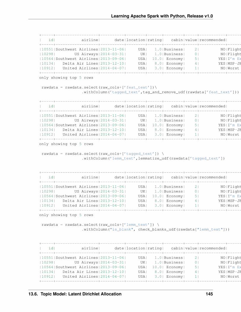
Learning Apache Spark with Python, Release v1.0
+-----+------------------+----------+--------+------+--------+-----+-----------+--------------------+--------------------+--------------------+| id| airline| date|location|rating| cabin|value|recommended| review| stop_text| feat_text|+-----+------------------+----------+--------+------+--------+-----+-----------+--------------------+--------------------+--------------------+|10551|Southwest Airlines|2013-11-06| USA| 1.0|Business| 2| NO|Flight 3246 from ...|flight 3246 chica...|flight chicago mi...||10298| US Airways|2014-03-31| UK| 1.0|Business| 0| NO|Flight from Manch...|flight manchester...|flight manchester...||10564|Southwest Airlines|2013-09-06| USA| 10.0| Economy| 5| YES|I’m Executive Pla...|i’m executive pla...|executive platinu...||10134| Delta Air Lines|2013-12-10| USA| 8.0| Economy| 4| YES|MSP-JFK-MXP and r...|msp-jfk-mxp retur...|msp jfk mxp retur...||10912| United Airlines|2014-04-07| USA| 3.0| Economy| 1| NO|Worst airline I h...|worst airline eve...|worst airline eve...|+-----+------------------+----------+--------+------+--------+-----+-----------+--------------------+--------------------+--------------------+only showing top 5 rows
rawdata = rawdata.select(raw_cols+[’feat_text’])\.withColumn(’tagged_text’,tag_and_remove_udf(rawdata[’feat_text’]))
+-----+------------------+----------+--------+------+--------+-----+-----------+--------------------+--------------------+--------------------+| id| airline| date|location|rating| cabin|value|recommended| review| feat_text| tagged_text|+-----+------------------+----------+--------+------+--------+-----+-----------+--------------------+--------------------+--------------------+|10551|Southwest Airlines|2013-11-06| USA| 1.0|Business| 2| NO|Flight 3246 from ...|flight chicago mi...| flight chicago m...||10298| US Airways|2014-03-31| UK| 1.0|Business| 0| NO|Flight from Manch...|flight manchester...| flight mancheste...||10564|Southwest Airlines|2013-09-06| USA| 10.0| Economy| 5| YES|I’m Executive Pla...|executive platinu...| executive platin...||10134| Delta Air Lines|2013-12-10| USA| 8.0| Economy| 4| YES|MSP-JFK-MXP and r...|msp jfk mxp retur...| msp jfk mxp retu...||10912| United Airlines|2014-04-07| USA| 3.0| Economy| 1| NO|Worst airline I h...|worst airline eve...| worst airline ua...|+-----+------------------+----------+--------+------+--------+-----+-----------+--------------------+--------------------+--------------------+only showing top 5 rows
rawdata = rawdata.select(raw_cols+[’tagged_text’]) \.withColumn(’lemm_text’,lemmatize_udf(rawdata[’tagged_text’])
+-----+------------------+----------+--------+------+--------+-----+-----------+--------------------+--------------------+--------------------+| id| airline| date|location|rating| cabin|value|recommended| review| tagged_text| lemm_text|+-----+------------------+----------+--------+------+--------+-----+-----------+--------------------+--------------------+--------------------+|10551|Southwest Airlines|2013-11-06| USA| 1.0|Business| 2| NO|Flight 3246 from ...| flight chicago m...|flight chicago mi...||10298| US Airways|2014-03-31| UK| 1.0|Business| 0| NO|Flight from Manch...| flight mancheste...|flight manchester...||10564|Southwest Airlines|2013-09-06| USA| 10.0| Economy| 5| YES|I’m Executive Pla...| executive platin...|executive platinu...||10134| Delta Air Lines|2013-12-10| USA| 8.0| Economy| 4| YES|MSP-JFK-MXP and r...| msp jfk mxp retu...|msp jfk mxp retur...||10912| United Airlines|2014-04-07| USA| 3.0| Economy| 1| NO|Worst airline I h...| worst airline ua...|worst airline ual...|+-----+------------------+----------+--------+------+--------+-----+-----------+--------------------+--------------------+--------------------+only showing top 5 rows
rawdata = rawdata.select(raw_cols+[’lemm_text’]) \.withColumn("is_blank", check_blanks_udf(rawdata["lemm_text"]))
+-----+------------------+----------+--------+------+--------+-----+-----------+--------------------+--------------------+--------+| id| airline| date|location|rating| cabin|value|recommended| review| lemm_text|is_blank|+-----+------------------+----------+--------+------+--------+-----+-----------+--------------------+--------------------+--------+|10551|Southwest Airlines|2013-11-06| USA| 1.0|Business| 2| NO|Flight 3246 from ...|flight chicago mi...| False||10298| US Airways|2014-03-31| UK| 1.0|Business| 0| NO|Flight from Manch...|flight manchester...| False||10564|Southwest Airlines|2013-09-06| USA| 10.0| Economy| 5| YES|I’m Executive Pla...|executive platinu...| False||10134| Delta Air Lines|2013-12-10| USA| 8.0| Economy| 4| YES|MSP-JFK-MXP and r...|msp jfk mxp retur...| False||10912| United Airlines|2014-04-07| USA| 3.0| Economy| 1| NO|Worst airline I h...|worst airline ual...| False|+-----+------------------+----------+--------+------+--------+-----+-----------+--------------------+--------------------+--------+
13.6. Topic Model: Latent Dirichlet Allocation 145
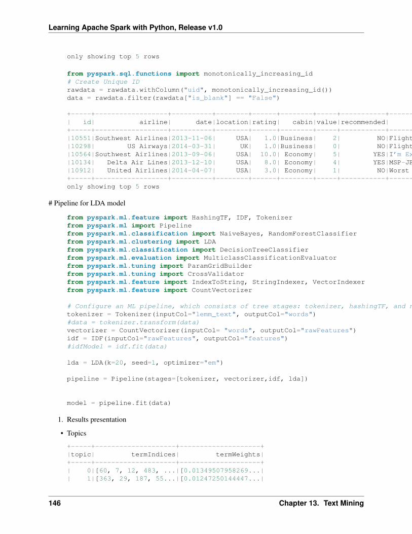
Learning Apache Spark with Python, Release v1.0
only showing top 5 rows
from pyspark.sql.functions import monotonically_increasing_id# Create Unique IDrawdata = rawdata.withColumn("uid", monotonically_increasing_id())data = rawdata.filter(rawdata["is_blank"] == "False")
+-----+------------------+----------+--------+------+--------+-----+-----------+--------------------+--------------------+--------+---+| id| airline| date|location|rating| cabin|value|recommended| review| lemm_text|is_blank|uid|+-----+------------------+----------+--------+------+--------+-----+-----------+--------------------+--------------------+--------+---+|10551|Southwest Airlines|2013-11-06| USA| 1.0|Business| 2| NO|Flight 3246 from ...|flight chicago mi...| False| 0||10298| US Airways|2014-03-31| UK| 1.0|Business| 0| NO|Flight from Manch...|flight manchester...| False| 1||10564|Southwest Airlines|2013-09-06| USA| 10.0| Economy| 5| YES|I’m Executive Pla...|executive platinu...| False| 2||10134| Delta Air Lines|2013-12-10| USA| 8.0| Economy| 4| YES|MSP-JFK-MXP and r...|msp jfk mxp retur...| False| 3||10912| United Airlines|2014-04-07| USA| 3.0| Economy| 1| NO|Worst airline I h...|worst airline ual...| False| 4|+-----+------------------+----------+--------+------+--------+-----+-----------+--------------------+--------------------+--------+---+only showing top 5 rows
# Pipeline for LDA model
from pyspark.ml.feature import HashingTF, IDF, Tokenizerfrom pyspark.ml import Pipelinefrom pyspark.ml.classification import NaiveBayes, RandomForestClassifierfrom pyspark.ml.clustering import LDAfrom pyspark.ml.classification import DecisionTreeClassifierfrom pyspark.ml.evaluation import MulticlassClassificationEvaluatorfrom pyspark.ml.tuning import ParamGridBuilderfrom pyspark.ml.tuning import CrossValidatorfrom pyspark.ml.feature import IndexToString, StringIndexer, VectorIndexerfrom pyspark.ml.feature import CountVectorizer
# Configure an ML pipeline, which consists of tree stages: tokenizer, hashingTF, and nb.tokenizer = Tokenizer(inputCol="lemm_text", outputCol="words")#data = tokenizer.transform(data)vectorizer = CountVectorizer(inputCol= "words", outputCol="rawFeatures")idf = IDF(inputCol="rawFeatures", outputCol="features")#idfModel = idf.fit(data)
lda = LDA(k=20, seed=1, optimizer="em")
pipeline = Pipeline(stages=[tokenizer, vectorizer,idf, lda])
model = pipeline.fit(data)
1. Results presentation
• Topics
+-----+--------------------+--------------------+|topic| termIndices| termWeights|+-----+--------------------+--------------------+| 0|[60, 7, 12, 483, ...|[0.01349507958269...|| 1|[363, 29, 187, 55...|[0.01247250144447...|
146 Chapter 13. Text Mining

Learning Apache Spark with Python, Release v1.0
| 2|[46, 107, 672, 27...|[0.01188684264641...|| 3|[76, 43, 285, 152...|[0.01132638300115...|| 4|[201, 13, 372, 69...|[0.01337529863256...|| 5|[122, 103, 181, 4...|[0.00930415977117...|| 6|[14, 270, 18, 74,...|[0.01253817708163...|| 7|[111, 36, 341, 10...|[0.01269584954257...|| 8|[477, 266, 297, 1...|[0.01017486869509...|| 9|[10, 73, 46, 1, 2...|[0.01050875237546...|| 10|[57, 29, 411, 10,...|[0.01777350667863...|| 11|[293, 119, 385, 4...|[0.01280305149305...|| 12|[116, 218, 256, 1...|[0.01570714218509...|| 13|[433, 171, 176, 3...|[0.00819684813575...|| 14|[74, 84, 45, 108,...|[0.01700630002172...|| 15|[669, 215, 14, 58...|[0.00779310974971...|| 16|[198, 21, 98, 164...|[0.01030577084202...|| 17|[96, 29, 569, 444...|[0.01297142577633...|| 18|[18, 60, 140, 64,...|[0.01306356985169...|| 19|[33, 178, 95, 2, ...|[0.00907425683229...|+-----+--------------------+--------------------+
• Topic terms
from pyspark.sql.types import ArrayType, StringType
def termsIdx2Term(vocabulary):def termsIdx2Term(termIndices):
return [vocabulary[int(index)] for index in termIndices]return udf(termsIdx2Term, ArrayType(StringType()))
vectorizerModel = model.stages[1]vocabList = vectorizerModel.vocabularyfinal = ldatopics.withColumn("Terms", termsIdx2Term(vocabList)("termIndices"))
+-----+------------------------------------------------+-------------------------------------------------------------------------------------+|topic|termIndices |Terms |+-----+------------------------------------------------+-------------------------------------------------------------------------------------+|0 |[60, 7, 12, 483, 292, 326, 88, 4, 808, 32] |[pm, plane, board, kid, online, lga, schedule, get, memphis, arrive] ||1 |[363, 29, 187, 55, 48, 647, 30, 9, 204, 457] |[dublin, class, th, sit, entertainment, express, say, delay, dl, son] ||2 |[46, 107, 672, 274, 92, 539, 23, 27, 279, 8] |[economy, sfo, milwaukee, decent, comfortable, iad, return, united, average, airline]||3 |[76, 43, 285, 152, 102, 34, 300, 113, 24, 31] |[didn, pay, lose, different, extra, bag, mile, baggage, leave, day] ||4 |[201, 13, 372, 692, 248, 62, 211, 187, 105, 110]|[houston, crew, heathrow, louisville, london, great, denver, th, land, jfk] ||5 |[122, 103, 181, 48, 434, 10, 121, 147, 934, 169]|[lhr, serve, screen, entertainment, ny, delta, excellent, atl, sin, newark] ||6 |[14, 270, 18, 74, 70, 37, 16, 450, 3, 20] |[check, employee, gate, line, change, wait, take, fll, time, tell] ||7 |[111, 36, 341, 10, 320, 528, 844, 19, 195, 524] |[atlanta, first, toilet, delta, washington, card, global, staff, route, amsterdam] ||8 |[477, 266, 297, 185, 1, 33, 22, 783, 17, 908] |[fuel, group, pas, boarding, seat, trip, minute, orleans, make, select] ||9 |[10, 73, 46, 1, 248, 302, 213, 659, 48, 228] |[delta, lax, economy, seat, london, detroit, comfo, weren, entertainment, wife] ||10 |[57, 29, 411, 10, 221, 121, 661, 19, 805, 733] |[business, class, fra, delta, lounge, excellent, syd, staff, nov, mexico] ||11 |[293, 119, 385, 481, 503, 69, 13, 87, 176, 545] |[march, ua, manchester, phx, envoy, drink, crew, american, aa, canada] ||12 |[116, 218, 256, 156, 639, 20, 365, 18, 22, 136] |[san, clt, francisco, second, text, tell, captain, gate, minute, available] ||13 |[433, 171, 176, 339, 429, 575, 10, 26, 474, 796]|[daughter, small, aa, ba, segment, proceed, delta, passenger, size, similar] ||14 |[74, 84, 45, 108, 342, 111, 315, 87, 52, 4] |[line, agent, next, hotel, standby, atlanta, dallas, american, book, get] ||15 |[669, 215, 14, 58, 561, 59, 125, 179, 93, 5] |[fit, carry, check, people, bathroom, ask, thing, row, don, fly] ||16 |[198, 21, 98, 164, 57, 141, 345, 62, 121, 174] |[ife, good, nice, much, business, lot, dfw, great, excellent, carrier] ||17 |[96, 29, 569, 444, 15, 568, 21, 103, 657, 505] |[phl, class, diego, lady, food, wheelchair, good, serve, miami, mia] |
13.6. Topic Model: Latent Dirichlet Allocation 147
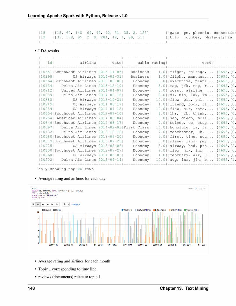
Learning Apache Spark with Python, Release v1.0
|18 |[18, 60, 140, 64, 47, 40, 31, 35, 2, 123] |[gate, pm, phoenix, connection, cancel, connect, day, airpo, hour, charlotte] ||19 |[33, 178, 95, 2, 9, 284, 42, 4, 89, 31] |[trip, counter, philadelphia, hour, delay, stay, way, get, southwest, day] |+-----+------------------------------------------------+-------------------------------------------------------------------------------------+
• LDA results
+-----+------------------+----------+-----------+------+--------------------+--------------------+--------------------+| id| airline| date| cabin|rating| words| features| topicDistribution|+-----+------------------+----------+-----------+------+--------------------+--------------------+--------------------+|10551|Southwest Airlines|2013-11-06| Business| 1.0|[flight, chicago,...|(4695,[0,2,3,6,11...|[0.03640342580508...||10298| US Airways|2014-03-31| Business| 1.0|[flight, manchest...|(4695,[0,1,2,6,7,...|[0.01381306271470...||10564|Southwest Airlines|2013-09-06| Economy| 10.0|[executive, plati...|(4695,[0,1,6,7,11...|[0.05063554352934...||10134| Delta Air Lines|2013-12-10| Economy| 8.0|[msp, jfk, mxp, r...|(4695,[0,1,3,10,1...|[0.01494708959842...||10912| United Airlines|2014-04-07| Economy| 3.0|[worst, airline, ...|(4695,[0,1,7,8,13...|[0.04421751181232...||10089| Delta Air Lines|2014-02-18| Economy| 2.0|[dl, mia, lax, im...|(4695,[2,4,5,7,8,...|[0.02158861273876...||10385| US Airways|2013-10-21| Economy| 10.0|[flew, gla, phl, ...|(4695,[0,1,3,5,14...|[0.03343845991816...||10249| US Airways|2014-06-17| Economy| 1.0|[friend, book, fl...|(4695,[0,2,3,4,5,...|[0.02362432562165...||10289| US Airways|2014-04-12| Economy| 10.0|[flew, air, rome,...|(4695,[0,1,5,8,13...|[0.01664012816210...||10654|Southwest Airlines|2012-07-10| Economy| 8.0|[lhr, jfk, think,...|(4695,[0,4,5,6,8,...|[0.01526072330297...||10754| American Airlines|2014-05-04| Economy| 10.0|[san, diego, moli...|(4695,[0,2,8,15,2...|[0.03571177612496...||10646|Southwest Airlines|2012-08-17| Economy| 7.0|[toledo, co, stop...|(4695,[0,2,3,4,7,...|[0.02394775146271...||10097| Delta Air Lines|2014-02-03|First Class| 10.0|[honolulu, la, fi...|(4695,[0,4,6,7,13...|[0.02008375619661...||10132| Delta Air Lines|2013-12-16| Economy| 7.0|[manchester, uk, ...|(4695,[0,1,2,3,5,...|[0.01463126146601...||10560|Southwest Airlines|2013-09-20| Economy| 9.0|[first, time, sou...|(4695,[0,3,7,8,9,...|[0.04934836409896...||10579|Southwest Airlines|2013-07-25| Economy| 0.0|[plane, land, pm,...|(4695,[2,3,4,5,7,...|[0.06106959241722...||10425| US Airways|2013-08-06| Economy| 3.0|[airway, bad, pro...|(4695,[2,3,4,7,8,...|[0.01770471771322...||10650|Southwest Airlines|2012-07-27| Economy| 9.0|[flew, jfk, lhr, ...|(4695,[0,1,6,13,1...|[0.02676226245086...||10260| US Airways|2014-06-03| Economy| 1.0|[february, air, u...|(4695,[0,2,4,17,2...|[0.02887390875079...||10202| Delta Air Lines|2013-09-14| Economy| 10.0|[aug, lhr, jfk, b...|(4695,[1,2,4,7,10...|[0.02377704988307...|+-----+------------------+----------+-----------+------+--------------------+--------------------+--------------------+only showing top 20 rows
• Average rating and airlines for each day
• Average rating and airlines for each month
• Topic 1 corresponding to time line
• reviews (documents) relate to topic 1
148 Chapter 13. Text Mining

Learning Apache Spark with Python, Release v1.0
13.6. Topic Model: Latent Dirichlet Allocation 149
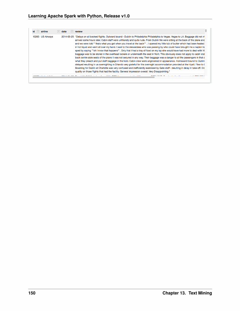
Learning Apache Spark with Python, Release v1.0
150 Chapter 13. Text Mining
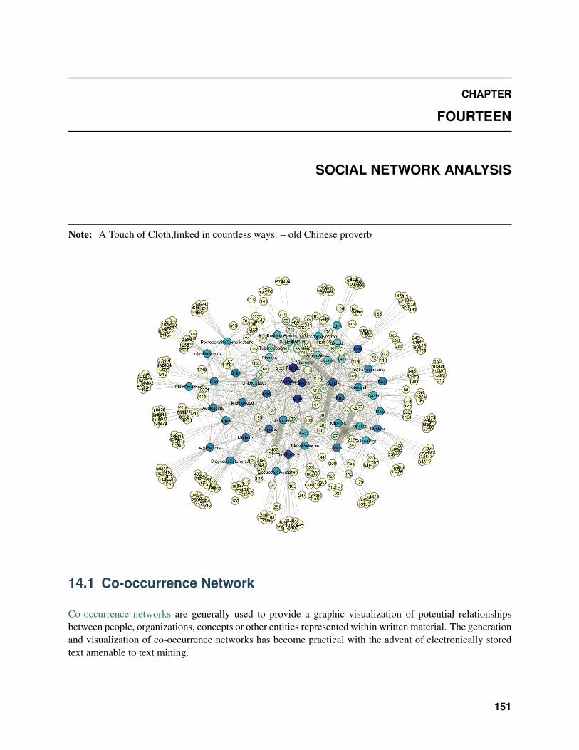
CHAPTER
FOURTEEN
SOCIAL NETWORK ANALYSIS
Note: A Touch of Cloth,linked in countless ways. – old Chinese proverb
14.1 Co-occurrence Network
Co-occurrence networks are generally used to provide a graphic visualization of potential relationshipsbetween people, organizations, concepts or other entities represented within written material. The generationand visualization of co-occurrence networks has become practical with the advent of electronically storedtext amenable to text mining.
151
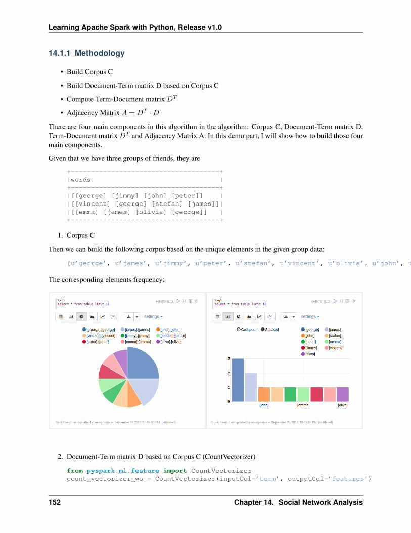
Learning Apache Spark with Python, Release v1.0
14.1.1 Methodology
• Build Corpus C
• Build Document-Term matrix D based on Corpus C
• Compute Term-Document matrix 𝐷𝑇
• Adjacency Matrix 𝐴 = 𝐷𝑇 ·𝐷
There are four main components in this algorithm in the algorithm: Corpus C, Document-Term matrix D,Term-Document matrix 𝐷𝑇 and Adjacency Matrix A. In this demo part, I will show how to build those fourmain components.
Given that we have three groups of friends, they are
+-------------------------------------+|words |+-------------------------------------+|[[george] [jimmy] [john] [peter]] ||[[vincent] [george] [stefan] [james]]||[[emma] [james] [olivia] [george]] |+-------------------------------------+
1. Corpus C
Then we can build the following corpus based on the unique elements in the given group data:
[u’george’, u’james’, u’jimmy’, u’peter’, u’stefan’, u’vincent’, u’olivia’, u’john’, u’emma’]
The corresponding elements frequency:
2. Document-Term matrix D based on Corpus C (CountVectorizer)
from pyspark.ml.feature import CountVectorizercount_vectorizer_wo = CountVectorizer(inputCol=’term’, outputCol=’features’)
152 Chapter 14. Social Network Analysis
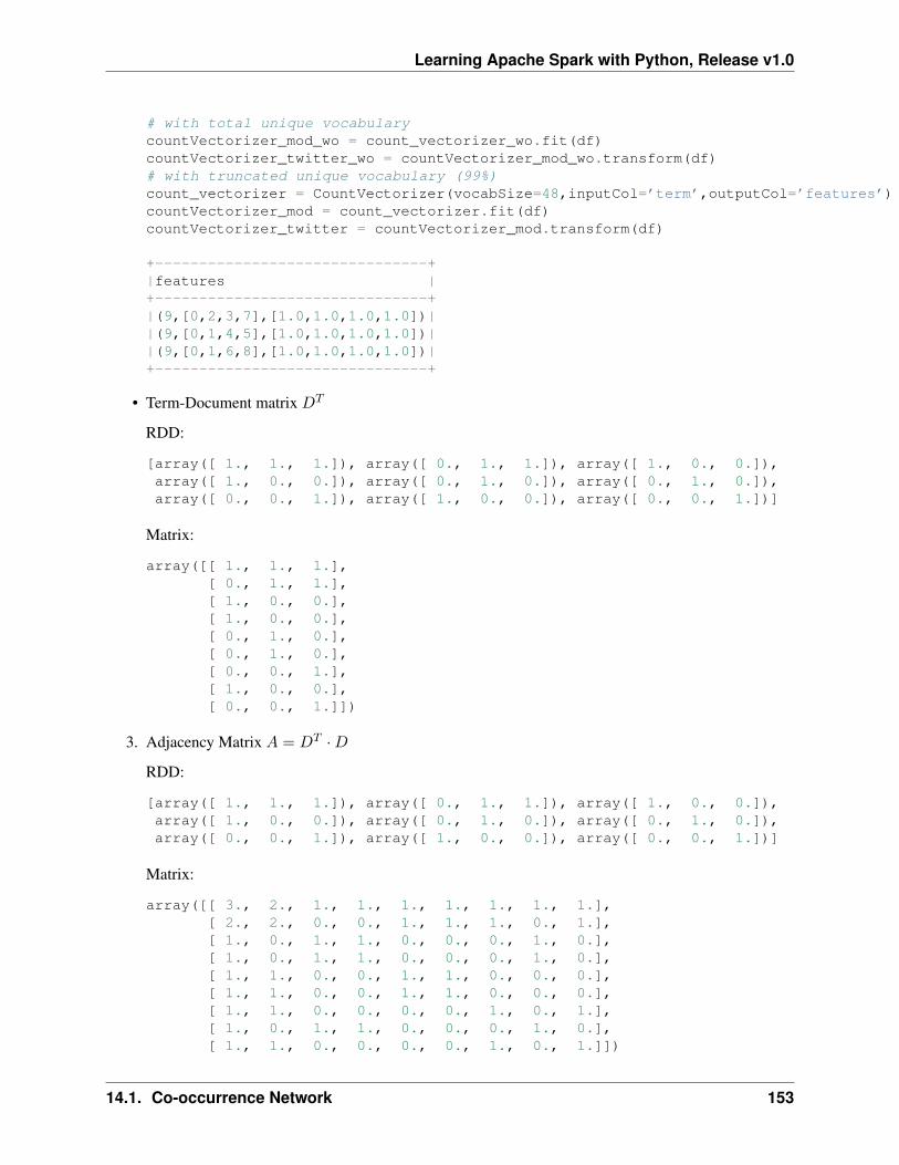
Learning Apache Spark with Python, Release v1.0
# with total unique vocabularycountVectorizer_mod_wo = count_vectorizer_wo.fit(df)countVectorizer_twitter_wo = countVectorizer_mod_wo.transform(df)# with truncated unique vocabulary (99%)count_vectorizer = CountVectorizer(vocabSize=48,inputCol=’term’,outputCol=’features’)countVectorizer_mod = count_vectorizer.fit(df)countVectorizer_twitter = countVectorizer_mod.transform(df)
+-------------------------------+|features |+-------------------------------+|(9,[0,2,3,7],[1.0,1.0,1.0,1.0])||(9,[0,1,4,5],[1.0,1.0,1.0,1.0])||(9,[0,1,6,8],[1.0,1.0,1.0,1.0])|+-------------------------------+
• Term-Document matrix 𝐷𝑇
RDD:
[array([ 1., 1., 1.]), array([ 0., 1., 1.]), array([ 1., 0., 0.]),array([ 1., 0., 0.]), array([ 0., 1., 0.]), array([ 0., 1., 0.]),array([ 0., 0., 1.]), array([ 1., 0., 0.]), array([ 0., 0., 1.])]
Matrix:
array([[ 1., 1., 1.],[ 0., 1., 1.],[ 1., 0., 0.],[ 1., 0., 0.],[ 0., 1., 0.],[ 0., 1., 0.],[ 0., 0., 1.],[ 1., 0., 0.],[ 0., 0., 1.]])
3. Adjacency Matrix 𝐴 = 𝐷𝑇 ·𝐷
RDD:
[array([ 1., 1., 1.]), array([ 0., 1., 1.]), array([ 1., 0., 0.]),array([ 1., 0., 0.]), array([ 0., 1., 0.]), array([ 0., 1., 0.]),array([ 0., 0., 1.]), array([ 1., 0., 0.]), array([ 0., 0., 1.])]
Matrix:
array([[ 3., 2., 1., 1., 1., 1., 1., 1., 1.],[ 2., 2., 0., 0., 1., 1., 1., 0., 1.],[ 1., 0., 1., 1., 0., 0., 0., 1., 0.],[ 1., 0., 1., 1., 0., 0., 0., 1., 0.],[ 1., 1., 0., 0., 1., 1., 0., 0., 0.],[ 1., 1., 0., 0., 1., 1., 0., 0., 0.],[ 1., 1., 0., 0., 0., 0., 1., 0., 1.],[ 1., 0., 1., 1., 0., 0., 0., 1., 0.],[ 1., 1., 0., 0., 0., 0., 1., 0., 1.]])
14.1. Co-occurrence Network 153
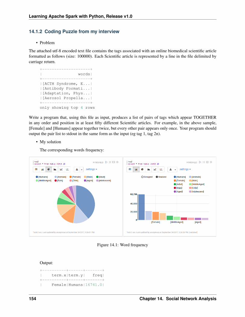
Learning Apache Spark with Python, Release v1.0
14.1.2 Coding Puzzle from my interview
• Problem
The attached utf-8 encoded text file contains the tags associated with an online biomedical scientific articleformatted as follows (size: 100000). Each Scientific article is represented by a line in the file delimited bycarriage return.
+--------------------+| words|+--------------------+|[ACTH Syndrome, E...||[Antibody Formati...||[Adaptation, Phys...||[Aerosol Propella...|+--------------------+only showing top 4 rows
Write a program that, using this file as input, produces a list of pairs of tags which appear TOGETHERin any order and position in at least fifty different Scientific articles. For example, in the above sample,[Female] and [Humans] appear together twice, but every other pair appears only once. Your program shouldoutput the pair list to stdout in the same form as the input (eg tag 1, tag 2n).
• My solution
The corresponding words frequency:
Figure 14.1: Word frequency
Output:
+----------+------+-------+| term.x|term.y| freq|+----------+------+-------+| Female|Humans|16741.0|
154 Chapter 14. Social Network Analysis
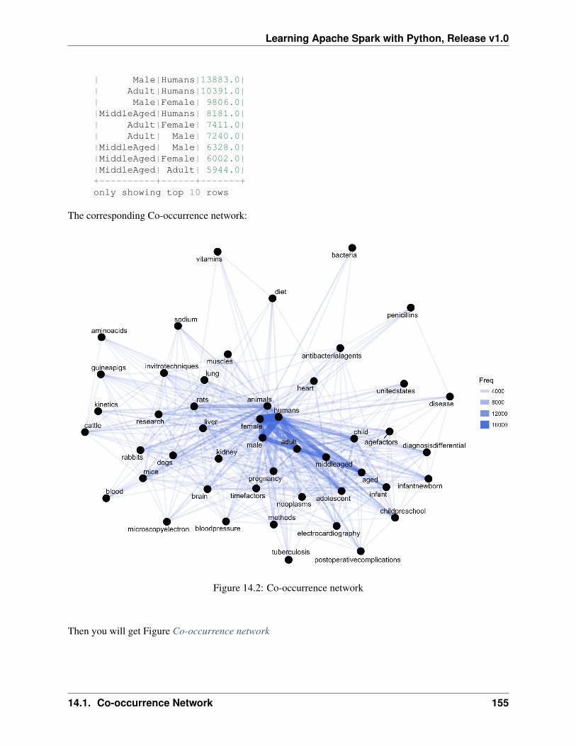
Learning Apache Spark with Python, Release v1.0
| Male|Humans|13883.0|| Adult|Humans|10391.0|| Male|Female| 9806.0||MiddleAged|Humans| 8181.0|| Adult|Female| 7411.0|| Adult| Male| 7240.0||MiddleAged| Male| 6328.0||MiddleAged|Female| 6002.0||MiddleAged| Adult| 5944.0|+----------+------+-------+only showing top 10 rows
The corresponding Co-occurrence network:
Figure 14.2: Co-occurrence network
Then you will get Figure Co-occurrence network
14.1. Co-occurrence Network 155

Learning Apache Spark with Python, Release v1.0
14.2 Correlation Network
156 Chapter 14. Social Network Analysis
CHAPTER
FIFTEEN
ALS: STOCK PORTFOLIO RECOMMENDATIONS
15.1 Recommender systems
Recommender systems or recommendation systems (sometimes replacing “system” with a synonym suchas platform or engine) are a subclass of information filtering system that seek to predict the “rating” or“preference” that a user would give to an item.”
The main idea is to build a matrix users R items rating values and try to factorize it, to recommend mainproducts rated by other users. A popular approach for this is matrix factorization is Alternating Least Squares(ALS)
15.2 Alternating Least Squares
Apache Spark ML implements ALS for collaborative filtering, a very popular algorithm for making recom-mendations.
ALS recommender is a matrix factorization algorithm that uses Alternating Least Squares with Weighted-Lamda-Regularization (ALS-WR). It factors the user to item matrix A into the user-to-feature matrix U andthe item-to-feature matrix M: It runs the ALS algorithm in a parallel fashion. The ALS algorithm shoulduncover the latent factors that explain the observed user to item ratings and tries to find optimal factorweights to minimize the least squares between predicted and actual ratings.
https://www.elenacuoco.com/2016/12/22/alternating-least-squares-als-spark-ml/
15.3 Demo
• The Jupyter notebook can be download from ALS Recommender systems.
• The data can be downloaf from German Credit.
15.3.1 Load and clean data
1. Set up spark context and SparkSession
157
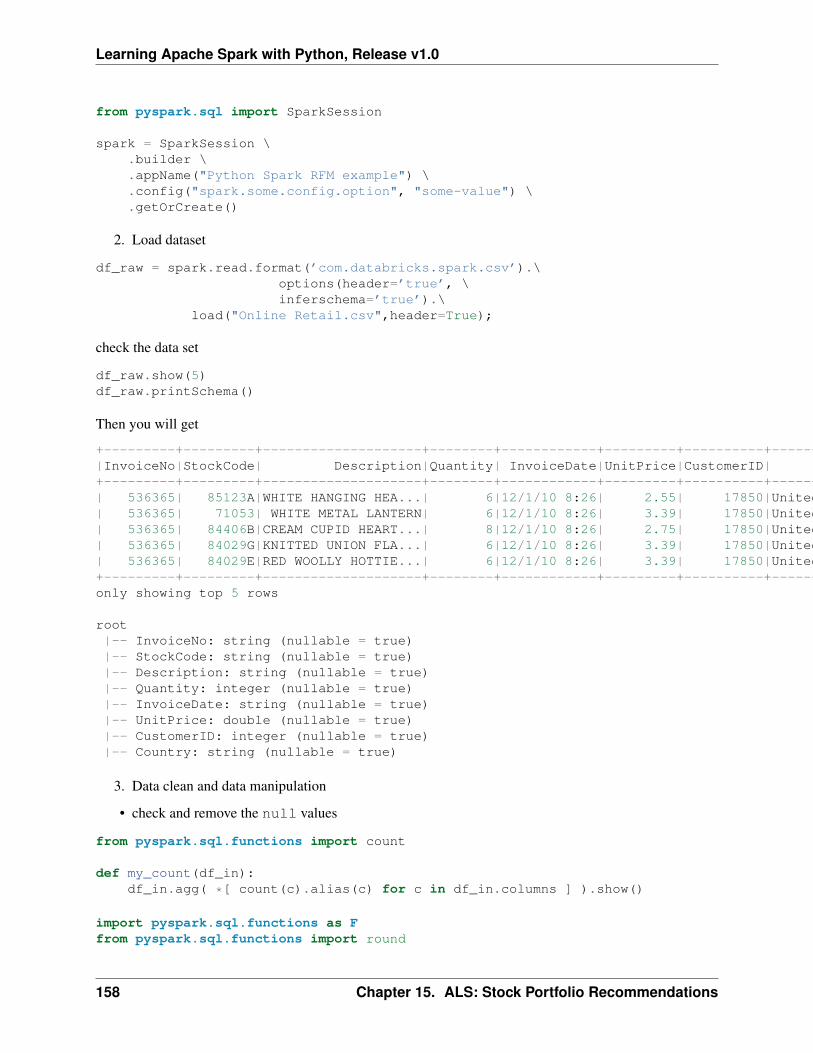
Learning Apache Spark with Python, Release v1.0
from pyspark.sql import SparkSession
spark = SparkSession \.builder \.appName("Python Spark RFM example") \.config("spark.some.config.option", "some-value") \.getOrCreate()
2. Load dataset
df_raw = spark.read.format(’com.databricks.spark.csv’).\options(header=’true’, \inferschema=’true’).\
load("Online Retail.csv",header=True);
check the data set
df_raw.show(5)df_raw.printSchema()
Then you will get
+---------+---------+--------------------+--------+------------+---------+----------+--------------+|InvoiceNo|StockCode| Description|Quantity| InvoiceDate|UnitPrice|CustomerID| Country|+---------+---------+--------------------+--------+------------+---------+----------+--------------+| 536365| 85123A|WHITE HANGING HEA...| 6|12/1/10 8:26| 2.55| 17850|United Kingdom|| 536365| 71053| WHITE METAL LANTERN| 6|12/1/10 8:26| 3.39| 17850|United Kingdom|| 536365| 84406B|CREAM CUPID HEART...| 8|12/1/10 8:26| 2.75| 17850|United Kingdom|| 536365| 84029G|KNITTED UNION FLA...| 6|12/1/10 8:26| 3.39| 17850|United Kingdom|| 536365| 84029E|RED WOOLLY HOTTIE...| 6|12/1/10 8:26| 3.39| 17850|United Kingdom|+---------+---------+--------------------+--------+------------+---------+----------+--------------+only showing top 5 rows
root|-- InvoiceNo: string (nullable = true)|-- StockCode: string (nullable = true)|-- Description: string (nullable = true)|-- Quantity: integer (nullable = true)|-- InvoiceDate: string (nullable = true)|-- UnitPrice: double (nullable = true)|-- CustomerID: integer (nullable = true)|-- Country: string (nullable = true)
3. Data clean and data manipulation
• check and remove the null values
from pyspark.sql.functions import count
def my_count(df_in):df_in.agg( *[ count(c).alias(c) for c in df_in.columns ] ).show()
import pyspark.sql.functions as Ffrom pyspark.sql.functions import round
158 Chapter 15. ALS: Stock Portfolio Recommendations
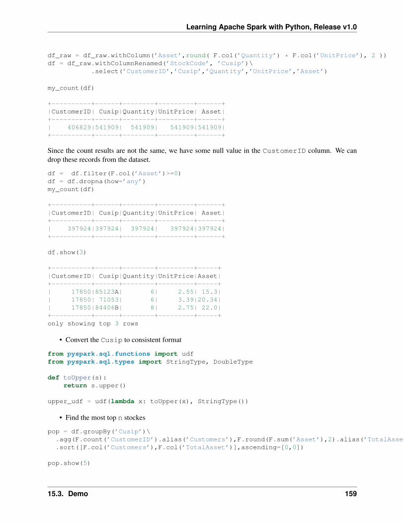
Learning Apache Spark with Python, Release v1.0
df_raw = df_raw.withColumn(’Asset’,round( F.col(’Quantity’) * F.col(’UnitPrice’), 2 ))df = df_raw.withColumnRenamed(’StockCode’, ’Cusip’)\
.select(’CustomerID’,’Cusip’,’Quantity’,’UnitPrice’,’Asset’)
my_count(df)
+----------+------+--------+---------+------+|CustomerID| Cusip|Quantity|UnitPrice| Asset|+----------+------+--------+---------+------+| 406829|541909| 541909| 541909|541909|+----------+------+--------+---------+------+
Since the count results are not the same, we have some null value in the CustomerID column. We candrop these records from the dataset.
df = df.filter(F.col(’Asset’)>=0)df = df.dropna(how=’any’)my_count(df)
+----------+------+--------+---------+------+|CustomerID| Cusip|Quantity|UnitPrice| Asset|+----------+------+--------+---------+------+| 397924|397924| 397924| 397924|397924|+----------+------+--------+---------+------+
df.show(3)
+----------+------+--------+---------+-----+|CustomerID| Cusip|Quantity|UnitPrice|Asset|+----------+------+--------+---------+-----+| 17850|85123A| 6| 2.55| 15.3|| 17850| 71053| 6| 3.39|20.34|| 17850|84406B| 8| 2.75| 22.0|+----------+------+--------+---------+-----+only showing top 3 rows
• Convert the Cusip to consistent format
from pyspark.sql.functions import udffrom pyspark.sql.types import StringType, DoubleType
def toUpper(s):return s.upper()
upper_udf = udf(lambda x: toUpper(x), StringType())
• Find the most top n stockes
pop = df.groupBy(’Cusip’)\.agg(F.count(’CustomerID’).alias(’Customers’),F.round(F.sum(’Asset’),2).alias(’TotalAsset’))\.sort([F.col(’Customers’),F.col(’TotalAsset’)],ascending=[0,0])
pop.show(5)
15.3. Demo 159
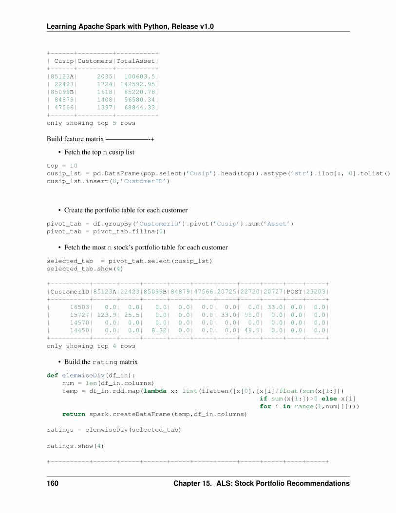
Learning Apache Spark with Python, Release v1.0
+------+---------+----------+| Cusip|Customers|TotalAsset|+------+---------+----------+|85123A| 2035| 100603.5|| 22423| 1724| 142592.95||85099B| 1618| 85220.78|| 84879| 1408| 56580.34|| 47566| 1397| 68844.33|+------+---------+----------+only showing top 5 rows
Build feature matrix ——————-+
• Fetch the top n cusip list
top = 10cusip_lst = pd.DataFrame(pop.select(’Cusip’).head(top)).astype(’str’).iloc[:, 0].tolist()cusip_lst.insert(0,’CustomerID’)
• Create the portfolio table for each customer
pivot_tab = df.groupBy(’CustomerID’).pivot(’Cusip’).sum(’Asset’)pivot_tab = pivot_tab.fillna(0)
• Fetch the most n stock’s portfolio table for each customer
selected_tab = pivot_tab.select(cusip_lst)selected_tab.show(4)
+----------+------+-----+------+-----+-----+-----+-----+-----+----+-----+|CustomerID|85123A|22423|85099B|84879|47566|20725|22720|20727|POST|23203|+----------+------+-----+------+-----+-----+-----+-----+-----+----+-----+| 16503| 0.0| 0.0| 0.0| 0.0| 0.0| 0.0| 0.0| 33.0| 0.0| 0.0|| 15727| 123.9| 25.5| 0.0| 0.0| 0.0| 33.0| 99.0| 0.0| 0.0| 0.0|| 14570| 0.0| 0.0| 0.0| 0.0| 0.0| 0.0| 0.0| 0.0| 0.0| 0.0|| 14450| 0.0| 0.0| 8.32| 0.0| 0.0| 0.0| 49.5| 0.0| 0.0| 0.0|+----------+------+-----+------+-----+-----+-----+-----+-----+----+-----+only showing top 4 rows
• Build the rating matrix
def elemwiseDiv(df_in):num = len(df_in.columns)temp = df_in.rdd.map(lambda x: list(flatten([x[0],[x[i]/float(sum(x[1:]))
if sum(x[1:])>0 else x[i]for i in range(1,num)]])))
return spark.createDataFrame(temp,df_in.columns)
ratings = elemwiseDiv(selected_tab)
ratings.show(4)
+----------+------+-----+------+-----+-----+-----+-----+-----+----+-----+
160 Chapter 15. ALS: Stock Portfolio Recommendations
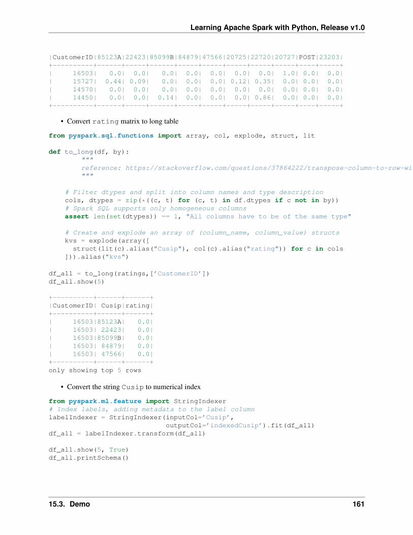
Learning Apache Spark with Python, Release v1.0
|CustomerID|85123A|22423|85099B|84879|47566|20725|22720|20727|POST|23203|+----------+------+-----+------+-----+-----+-----+-----+-----+----+-----+| 16503| 0.0| 0.0| 0.0| 0.0| 0.0| 0.0| 0.0| 1.0| 0.0| 0.0|| 15727| 0.44| 0.09| 0.0| 0.0| 0.0| 0.12| 0.35| 0.0| 0.0| 0.0|| 14570| 0.0| 0.0| 0.0| 0.0| 0.0| 0.0| 0.0| 0.0| 0.0| 0.0|| 14450| 0.0| 0.0| 0.14| 0.0| 0.0| 0.0| 0.86| 0.0| 0.0| 0.0|+----------+------+-----+------+-----+-----+-----+-----+-----+----+-----+
• Convert rating matrix to long table
from pyspark.sql.functions import array, col, explode, struct, lit
def to_long(df, by):"""reference: https://stackoverflow.com/questions/37864222/transpose-column-to-row-with-spark"""
# Filter dtypes and split into column names and type descriptioncols, dtypes = zip(*((c, t) for (c, t) in df.dtypes if c not in by))# Spark SQL supports only homogeneous columnsassert len(set(dtypes)) == 1, "All columns have to be of the same type"
# Create and explode an array of (column_name, column_value) structskvs = explode(array([
struct(lit(c).alias("Cusip"), col(c).alias("rating")) for c in cols])).alias("kvs")
df_all = to_long(ratings,[’CustomerID’])df_all.show(5)
+----------+------+------+|CustomerID| Cusip|rating|+----------+------+------+| 16503|85123A| 0.0|| 16503| 22423| 0.0|| 16503|85099B| 0.0|| 16503| 84879| 0.0|| 16503| 47566| 0.0|+----------+------+------+only showing top 5 rows
• Convert the string Cusip to numerical index
from pyspark.ml.feature import StringIndexer# Index labels, adding metadata to the label columnlabelIndexer = StringIndexer(inputCol=’Cusip’,
outputCol=’indexedCusip’).fit(df_all)df_all = labelIndexer.transform(df_all)
df_all.show(5, True)df_all.printSchema()
15.3. Demo 161
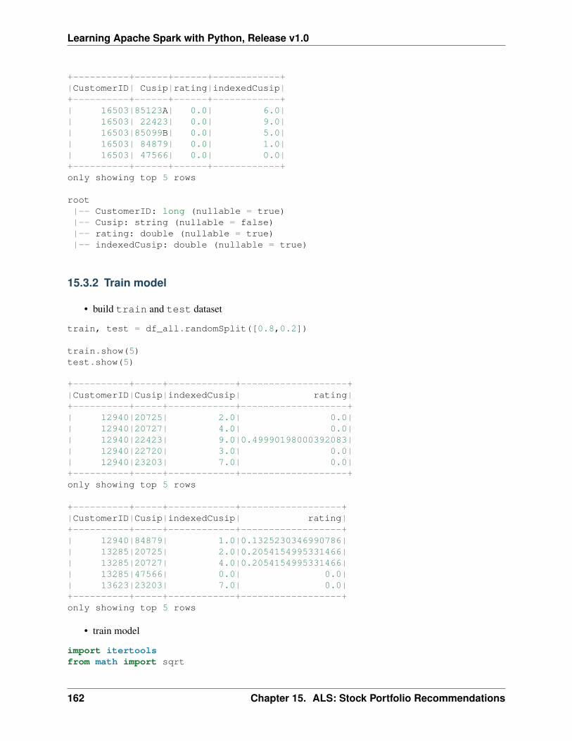
Learning Apache Spark with Python, Release v1.0
+----------+------+------+------------+|CustomerID| Cusip|rating|indexedCusip|+----------+------+------+------------+| 16503|85123A| 0.0| 6.0|| 16503| 22423| 0.0| 9.0|| 16503|85099B| 0.0| 5.0|| 16503| 84879| 0.0| 1.0|| 16503| 47566| 0.0| 0.0|+----------+------+------+------------+only showing top 5 rows
root|-- CustomerID: long (nullable = true)|-- Cusip: string (nullable = false)|-- rating: double (nullable = true)|-- indexedCusip: double (nullable = true)
15.3.2 Train model
• build train and test dataset
train, test = df_all.randomSplit([0.8,0.2])
train.show(5)test.show(5)
+----------+-----+------------+-------------------+|CustomerID|Cusip|indexedCusip| rating|+----------+-----+------------+-------------------+| 12940|20725| 2.0| 0.0|| 12940|20727| 4.0| 0.0|| 12940|22423| 9.0|0.49990198000392083|| 12940|22720| 3.0| 0.0|| 12940|23203| 7.0| 0.0|+----------+-----+------------+-------------------+only showing top 5 rows
+----------+-----+------------+------------------+|CustomerID|Cusip|indexedCusip| rating|+----------+-----+------------+------------------+| 12940|84879| 1.0|0.1325230346990786|| 13285|20725| 2.0|0.2054154995331466|| 13285|20727| 4.0|0.2054154995331466|| 13285|47566| 0.0| 0.0|| 13623|23203| 7.0| 0.0|+----------+-----+------------+------------------+only showing top 5 rows
• train model
import itertoolsfrom math import sqrt
162 Chapter 15. ALS: Stock Portfolio Recommendations
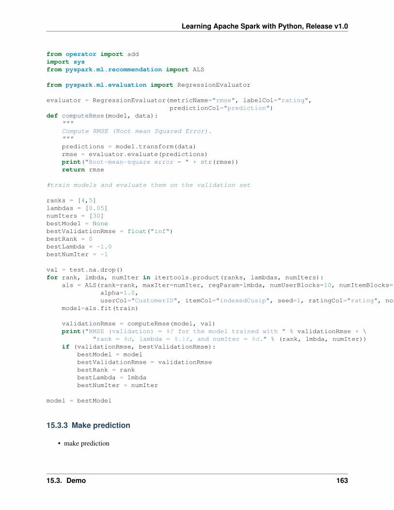
Learning Apache Spark with Python, Release v1.0
from operator import addimport sysfrom pyspark.ml.recommendation import ALS
from pyspark.ml.evaluation import RegressionEvaluator
evaluator = RegressionEvaluator(metricName="rmse", labelCol="rating",predictionCol="prediction")
def computeRmse(model, data):"""Compute RMSE (Root mean Squared Error)."""predictions = model.transform(data)rmse = evaluator.evaluate(predictions)print("Root-mean-square error = " + str(rmse))return rmse
#train models and evaluate them on the validation set
ranks = [4,5]lambdas = [0.05]numIters = [30]bestModel = NonebestValidationRmse = float("inf")bestRank = 0bestLambda = -1.0bestNumIter = -1
val = test.na.drop()for rank, lmbda, numIter in itertools.product(ranks, lambdas, numIters):
als = ALS(rank=rank, maxIter=numIter, regParam=lmbda, numUserBlocks=10, numItemBlocks=10, implicitPrefs=False,alpha=1.0,userCol="CustomerID", itemCol="indexedCusip", seed=1, ratingCol="rating", nonnegative=True)
model=als.fit(train)
validationRmse = computeRmse(model, val)print("RMSE (validation) = %f for the model trained with " % validationRmse + \
"rank = %d, lambda = %.1f, and numIter = %d." % (rank, lmbda, numIter))if (validationRmse, bestValidationRmse):
bestModel = modelbestValidationRmse = validationRmsebestRank = rankbestLambda = lmbdabestNumIter = numIter
model = bestModel
15.3.3 Make prediction
• make prediction
15.3. Demo 163
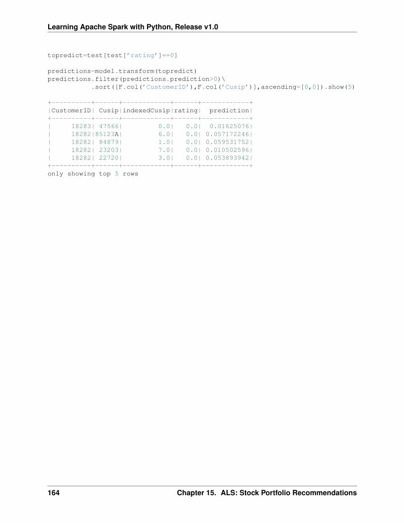
Learning Apache Spark with Python, Release v1.0
topredict=test[test[’rating’]==0]
predictions=model.transform(topredict)predictions.filter(predictions.prediction>0)\
.sort([F.col(’CustomerID’),F.col(’Cusip’)],ascending=[0,0]).show(5)
+----------+------+------------+------+------------+|CustomerID| Cusip|indexedCusip|rating| prediction|+----------+------+------------+------+------------+| 18283| 47566| 0.0| 0.0| 0.01625076|| 18282|85123A| 6.0| 0.0| 0.057172246|| 18282| 84879| 1.0| 0.0| 0.059531752|| 18282| 23203| 7.0| 0.0| 0.010502596|| 18282| 22720| 3.0| 0.0| 0.053893942|+----------+------+------------+------+------------+only showing top 5 rows
164 Chapter 15. ALS: Stock Portfolio Recommendations
CHAPTER
SIXTEEN
MONTE CARLO SIMULATION
Monte Carlo simulations are just a way of estimating a fixed parameter by repeatedly generating randomnumbers. More details can be found at ‘A Zero Math Introduction to Markov Chain Monte CarloMethods‘_.
Monte Carlo simulation is a technique used to understand the impact of risk and uncertainty in financial,project management, cost, and other forecasting models. A Monte Carlo simulator helps one visualize mostor all of the potential outcomes to have a better idea regarding the risk of a decision. More details can befound at The house always wins.
16.1 Simulating Casino Win
We assume that the player John has the 49% chance to win the game and the wager will be $5 per game.
import numpy as npimport pandas as pdimport matplotlib.pyplot as plt
start_m =100wager = 5bets = 100trials = 1000
trans = np.vectorize(lambda t: -wager if t <=0.51 else wager)
fig = plt.figure(figsize=(10, 6))ax = fig.add_subplot(1,1,1)
end_m = []
for i in range(trials):money = reduce(lambda c, x: c + [c[-1] + x], trans(np.random.random(bets)), [start_m])end_m.append(money[-1])plt.plot(money)
plt.ylabel(’Player Money in $’)plt.xlabel(’Number of bets’)plt.title(("John starts the game with $ %.2f and ends with $ %.2f")%(start_m,sum(end_m)/len(end_m)))plt.show()
165
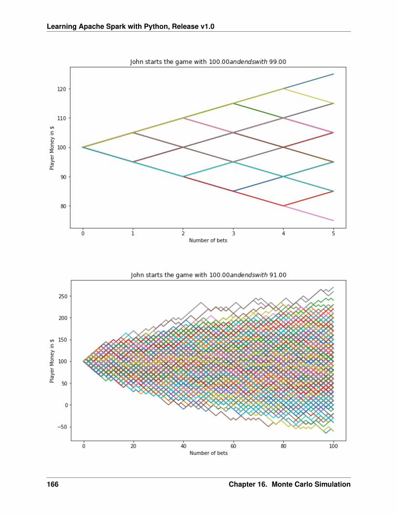
Learning Apache Spark with Python, Release v1.0
166 Chapter 16. Monte Carlo Simulation
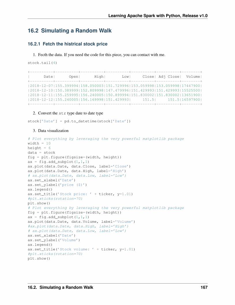
Learning Apache Spark with Python, Release v1.0
16.2 Simulating a Random Walk
16.2.1 Fetch the histrical stock price
1. Fecth the data. If you need the code for this piece, you can contact with me.
stock.tail(4)
+----------+----------+----------+----------+----------+----------+--------+| Date| Open| High| Low| Close| Adj Close| Volume|+----------+----------+----------+----------+----------+----------+--------+|2018-12-07|155.399994|158.050003|151.729996|153.059998|153.059998|17447900||2018-12-10|150.389999|152.809998|147.479996|151.429993|151.429993|15525500||2018-12-11|155.259995|156.240005|150.899994|151.830002|151.830002|13651900||2018-12-12|155.240005|156.169998|151.429993| 151.5| 151.5|16597900|+----------+----------+----------+----------+----------+----------+--------+
2. Convert the str type date to date type
stock[’Date’] = pd.to_datetime(stock[’Date’])
3. Data visualization
# Plot everything by leveraging the very powerful matplotlib packagewidth = 10height = 6data = stockfig = plt.figure(figsize=(width, height))ax = fig.add_subplot(1,1,1)ax.plot(data.Date, data.Close, label=’Close’)ax.plot(data.Date, data.High, label=’High’)# ax.plot(data.Date, data.Low, label=’Low’)ax.set_xlabel(’Date’)ax.set_ylabel(’price ($)’)ax.legend()ax.set_title(’Stock price: ’ + ticker, y=1.01)#plt.xticks(rotation=70)plt.show()# Plot everything by leveraging the very powerful matplotlib packagefig = plt.figure(figsize=(width, height))ax = fig.add_subplot(1,1,1)ax.plot(data.Date, data.Volume, label=’Volume’)#ax.plot(data.Date, data.High, label=’High’)# ax.plot(data.Date, data.Low, label=’Low’)ax.set_xlabel(’Date’)ax.set_ylabel(’Volume’)ax.legend()ax.set_title(’Stock volume: ’ + ticker, y=1.01)#plt.xticks(rotation=70)plt.show()
16.2. Simulating a Random Walk 167
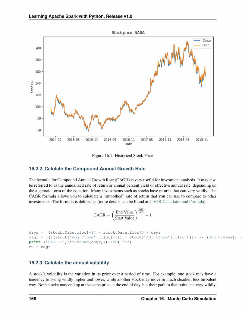
Learning Apache Spark with Python, Release v1.0
Figure 16.1: Historical Stock Price
16.2.2 Calulate the Compound Annual Growth Rate
The formula for Compound Annual Growth Rate (CAGR) is very useful for investment analysis. It may alsobe referred to as the annualized rate of return or annual percent yield or effective annual rate, depending onthe algebraic form of the equation. Many investments such as stocks have returns that can vary wildly. TheCAGR formula allows you to calculate a “smoothed” rate of return that you can use to compare to otherinvestments. The formula is defined as (more details can be found at CAGR Calculator and Formula)
CAGR =
(︂End ValueStart Value
)︂ 365Days
− 1
days = (stock.Date.iloc[-1] - stock.Date.iloc[0]).dayscagr = ((((stock[’Adj Close’].iloc[-1]) / stock[’Adj Close’].iloc[0])) ** (365.0/days)) - 1print (’CAGR =’,str(round(cagr,4)*100)+"%")mu = cagr
16.2.3 Calulate the annual volatility
A stock’s volatility is the variation in its price over a period of time. For example, one stock may have atendency to swing wildly higher and lower, while another stock may move in much steadier, less turbulentway. Both stocks may end up at the same price at the end of day, but their path to that point can vary wildly.
168 Chapter 16. Monte Carlo Simulation
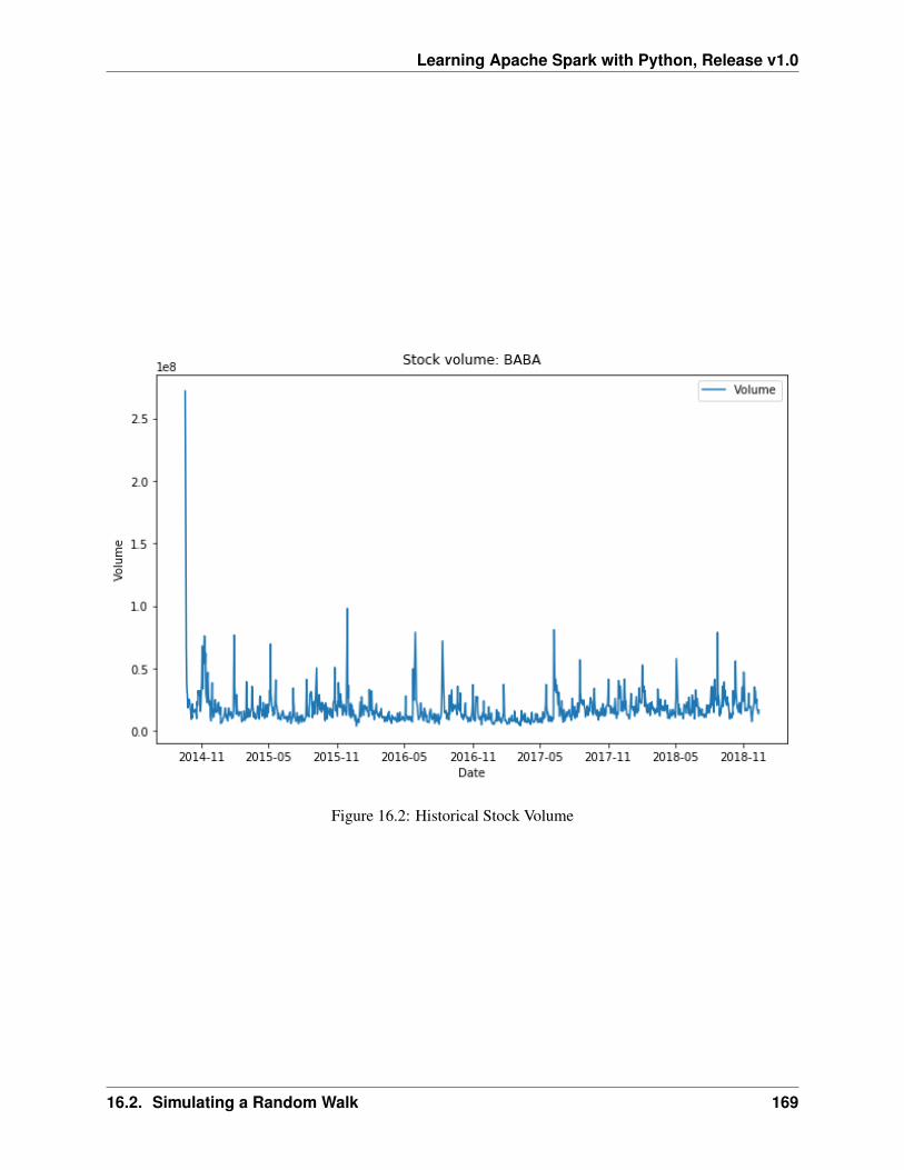
Learning Apache Spark with Python, Release v1.0
Figure 16.2: Historical Stock Volume
16.2. Simulating a Random Walk 169
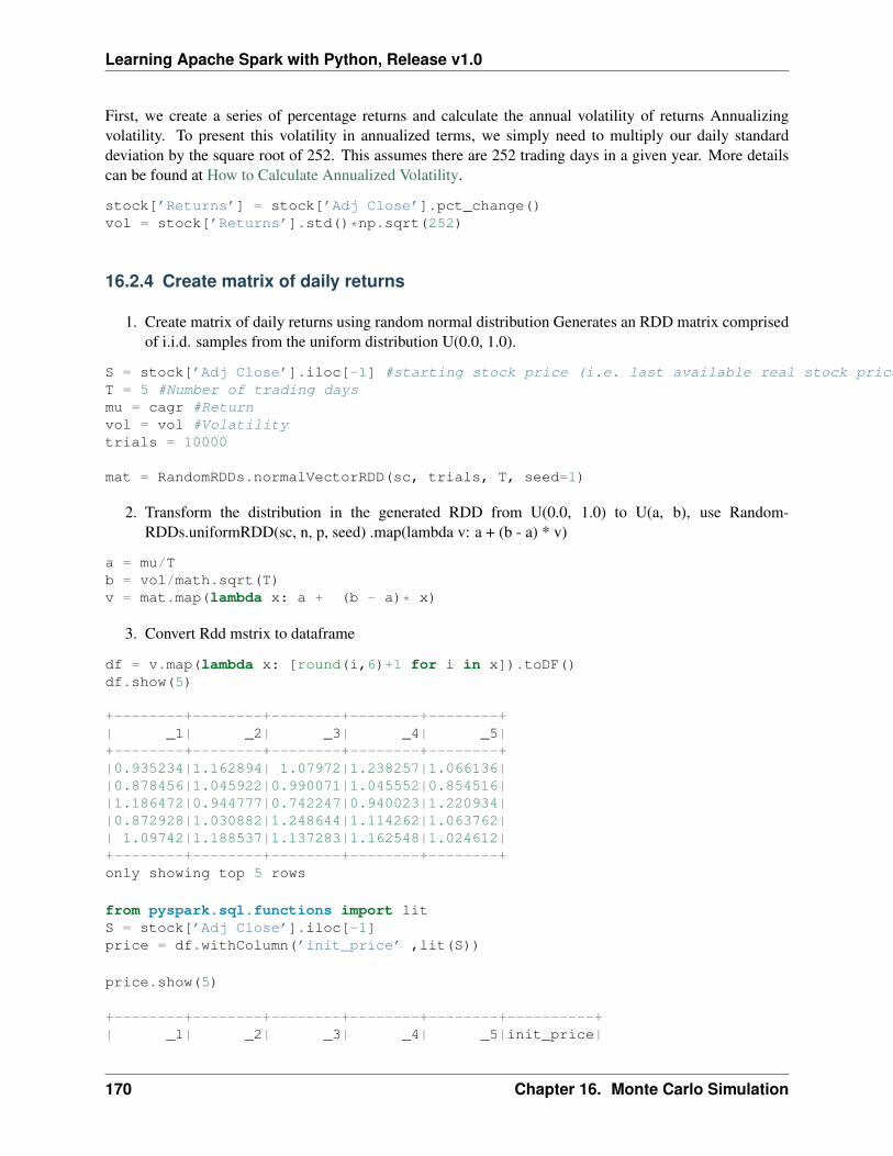
Learning Apache Spark with Python, Release v1.0
First, we create a series of percentage returns and calculate the annual volatility of returns Annualizingvolatility. To present this volatility in annualized terms, we simply need to multiply our daily standarddeviation by the square root of 252. This assumes there are 252 trading days in a given year. More detailscan be found at How to Calculate Annualized Volatility.
stock[’Returns’] = stock[’Adj Close’].pct_change()vol = stock[’Returns’].std()*np.sqrt(252)
16.2.4 Create matrix of daily returns
1. Create matrix of daily returns using random normal distribution Generates an RDD matrix comprisedof i.i.d. samples from the uniform distribution U(0.0, 1.0).
S = stock[’Adj Close’].iloc[-1] #starting stock price (i.e. last available real stock price)T = 5 #Number of trading daysmu = cagr #Returnvol = vol #Volatilitytrials = 10000
mat = RandomRDDs.normalVectorRDD(sc, trials, T, seed=1)
2. Transform the distribution in the generated RDD from U(0.0, 1.0) to U(a, b), use Random-RDDs.uniformRDD(sc, n, p, seed) .map(lambda v: a + (b - a) * v)
a = mu/Tb = vol/math.sqrt(T)v = mat.map(lambda x: a + (b - a)* x)
3. Convert Rdd mstrix to dataframe
df = v.map(lambda x: [round(i,6)+1 for i in x]).toDF()df.show(5)
+--------+--------+--------+--------+--------+| _1| _2| _3| _4| _5|+--------+--------+--------+--------+--------+|0.935234|1.162894| 1.07972|1.238257|1.066136||0.878456|1.045922|0.990071|1.045552|0.854516||1.186472|0.944777|0.742247|0.940023|1.220934||0.872928|1.030882|1.248644|1.114262|1.063762|| 1.09742|1.188537|1.137283|1.162548|1.024612|+--------+--------+--------+--------+--------+only showing top 5 rows
from pyspark.sql.functions import litS = stock[’Adj Close’].iloc[-1]price = df.withColumn(’init_price’ ,lit(S))
price.show(5)
+--------+--------+--------+--------+--------+----------+| _1| _2| _3| _4| _5|init_price|
170 Chapter 16. Monte Carlo Simulation
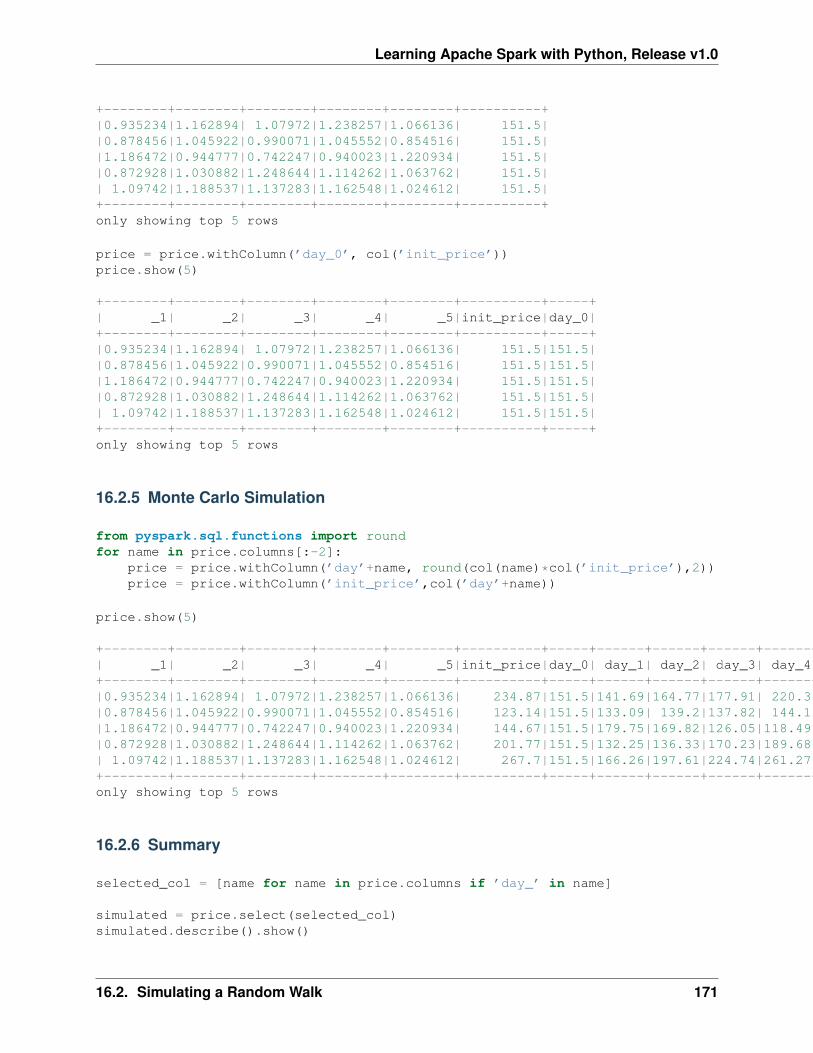
Learning Apache Spark with Python, Release v1.0
+--------+--------+--------+--------+--------+----------+|0.935234|1.162894| 1.07972|1.238257|1.066136| 151.5||0.878456|1.045922|0.990071|1.045552|0.854516| 151.5||1.186472|0.944777|0.742247|0.940023|1.220934| 151.5||0.872928|1.030882|1.248644|1.114262|1.063762| 151.5|| 1.09742|1.188537|1.137283|1.162548|1.024612| 151.5|+--------+--------+--------+--------+--------+----------+only showing top 5 rows
price = price.withColumn(’day_0’, col(’init_price’))price.show(5)
+--------+--------+--------+--------+--------+----------+-----+| _1| _2| _3| _4| _5|init_price|day_0|+--------+--------+--------+--------+--------+----------+-----+|0.935234|1.162894| 1.07972|1.238257|1.066136| 151.5|151.5||0.878456|1.045922|0.990071|1.045552|0.854516| 151.5|151.5||1.186472|0.944777|0.742247|0.940023|1.220934| 151.5|151.5||0.872928|1.030882|1.248644|1.114262|1.063762| 151.5|151.5|| 1.09742|1.188537|1.137283|1.162548|1.024612| 151.5|151.5|+--------+--------+--------+--------+--------+----------+-----+only showing top 5 rows
16.2.5 Monte Carlo Simulation
from pyspark.sql.functions import roundfor name in price.columns[:-2]:
price = price.withColumn(’day’+name, round(col(name)*col(’init_price’),2))price = price.withColumn(’init_price’,col(’day’+name))
price.show(5)
+--------+--------+--------+--------+--------+----------+-----+------+------+------+------+------+| _1| _2| _3| _4| _5|init_price|day_0| day_1| day_2| day_3| day_4| day_5|+--------+--------+--------+--------+--------+----------+-----+------+------+------+------+------+|0.935234|1.162894| 1.07972|1.238257|1.066136| 234.87|151.5|141.69|164.77|177.91| 220.3|234.87||0.878456|1.045922|0.990071|1.045552|0.854516| 123.14|151.5|133.09| 139.2|137.82| 144.1|123.14||1.186472|0.944777|0.742247|0.940023|1.220934| 144.67|151.5|179.75|169.82|126.05|118.49|144.67||0.872928|1.030882|1.248644|1.114262|1.063762| 201.77|151.5|132.25|136.33|170.23|189.68|201.77|| 1.09742|1.188537|1.137283|1.162548|1.024612| 267.7|151.5|166.26|197.61|224.74|261.27| 267.7|+--------+--------+--------+--------+--------+----------+-----+------+------+------+------+------+only showing top 5 rows
16.2.6 Summary
selected_col = [name for name in price.columns if ’day_’ in name]
simulated = price.select(selected_col)simulated.describe().show()
16.2. Simulating a Random Walk 171
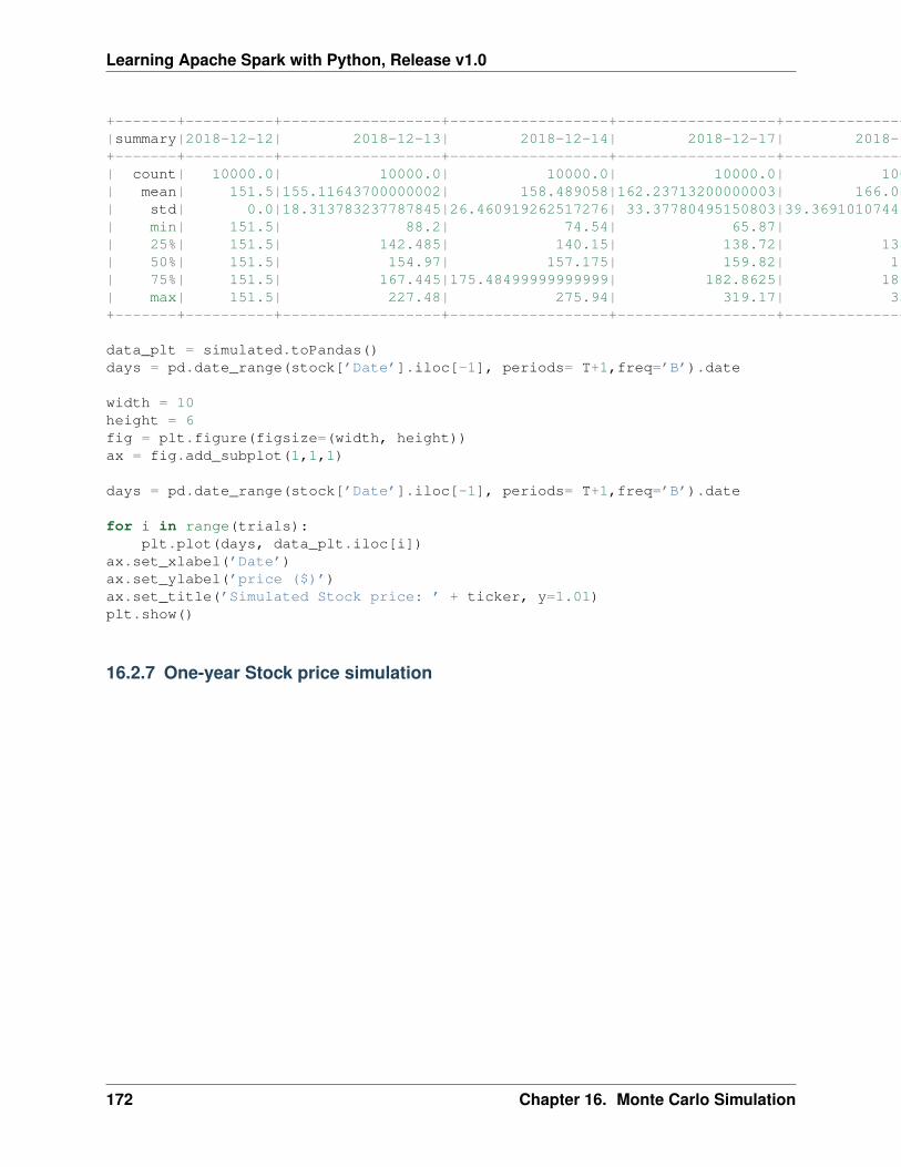
Learning Apache Spark with Python, Release v1.0
+-------+----------+------------------+------------------+------------------+------------------+------------------+|summary|2018-12-12| 2018-12-13| 2018-12-14| 2018-12-17| 2018-12-18| 2018-12-19|+-------+----------+------------------+------------------+------------------+------------------+------------------+| count| 10000.0| 10000.0| 10000.0| 10000.0| 10000.0| 10000.0|| mean| 151.5|155.11643700000002| 158.489058|162.23713200000003| 166.049375| 170.006525|| std| 0.0|18.313783237787845|26.460919262517276| 33.37780495150803|39.369101074463416|45.148120695490846|| min| 151.5| 88.2| 74.54| 65.87| 68.21| 58.25|| 25%| 151.5| 142.485| 140.15| 138.72| 138.365| 137.33|| 50%| 151.5| 154.97| 157.175| 159.82| 162.59|165.04500000000002|| 75%| 151.5| 167.445|175.48499999999999| 182.8625| 189.725| 196.975|| max| 151.5| 227.48| 275.94| 319.17| 353.59| 403.68|+-------+----------+------------------+------------------+------------------+------------------+------------------+
data_plt = simulated.toPandas()days = pd.date_range(stock[’Date’].iloc[-1], periods= T+1,freq=’B’).date
width = 10height = 6fig = plt.figure(figsize=(width, height))ax = fig.add_subplot(1,1,1)
days = pd.date_range(stock[’Date’].iloc[-1], periods= T+1,freq=’B’).date
for i in range(trials):plt.plot(days, data_plt.iloc[i])
ax.set_xlabel(’Date’)ax.set_ylabel(’price ($)’)ax.set_title(’Simulated Stock price: ’ + ticker, y=1.01)plt.show()
16.2.7 One-year Stock price simulation
172 Chapter 16. Monte Carlo Simulation
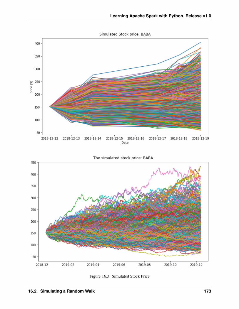
Learning Apache Spark with Python, Release v1.0
Figure 16.3: Simulated Stock Price
16.2. Simulating a Random Walk 173
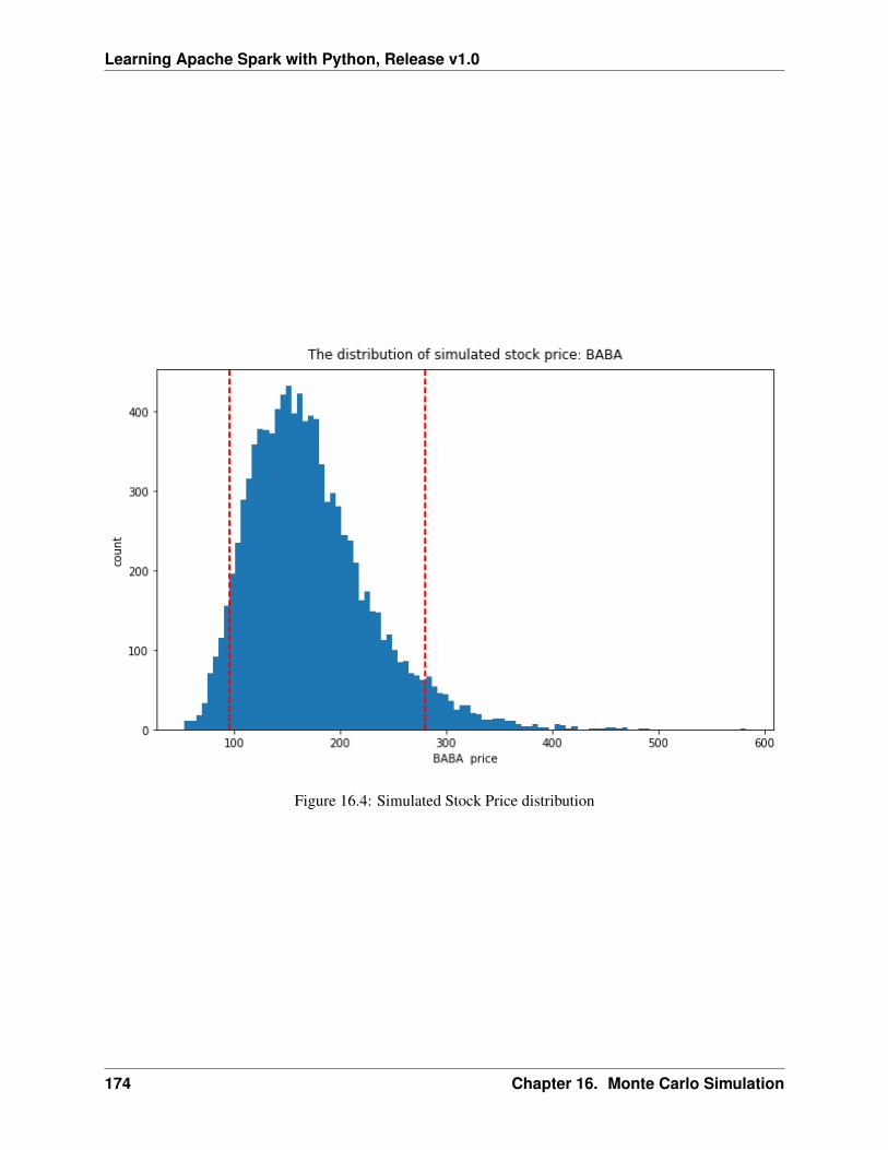
Learning Apache Spark with Python, Release v1.0
Figure 16.4: Simulated Stock Price distribution
174 Chapter 16. Monte Carlo Simulation

CHAPTER
SEVENTEEN
MARKOV CHAIN MONTE CARLO
Monte Carlo simulations are just a way of estimating a fixed parameter by repeatedly generating randomnumbers. More details can be found at A Zero Math Introduction to Markov Chain Monte Carlo Methods.
Markov Chain Monte Carlo (MCMC) methods are used to approximate the posterior distribution of a pa-rameter of interest by random sampling in a probabilistic space. More details can be found at A Zero MathIntroduction to Markov Chain Monte Carlo Methods.
175
Learning Apache Spark with Python, Release v1.0
176 Chapter 17. Markov Chain Monte Carlo
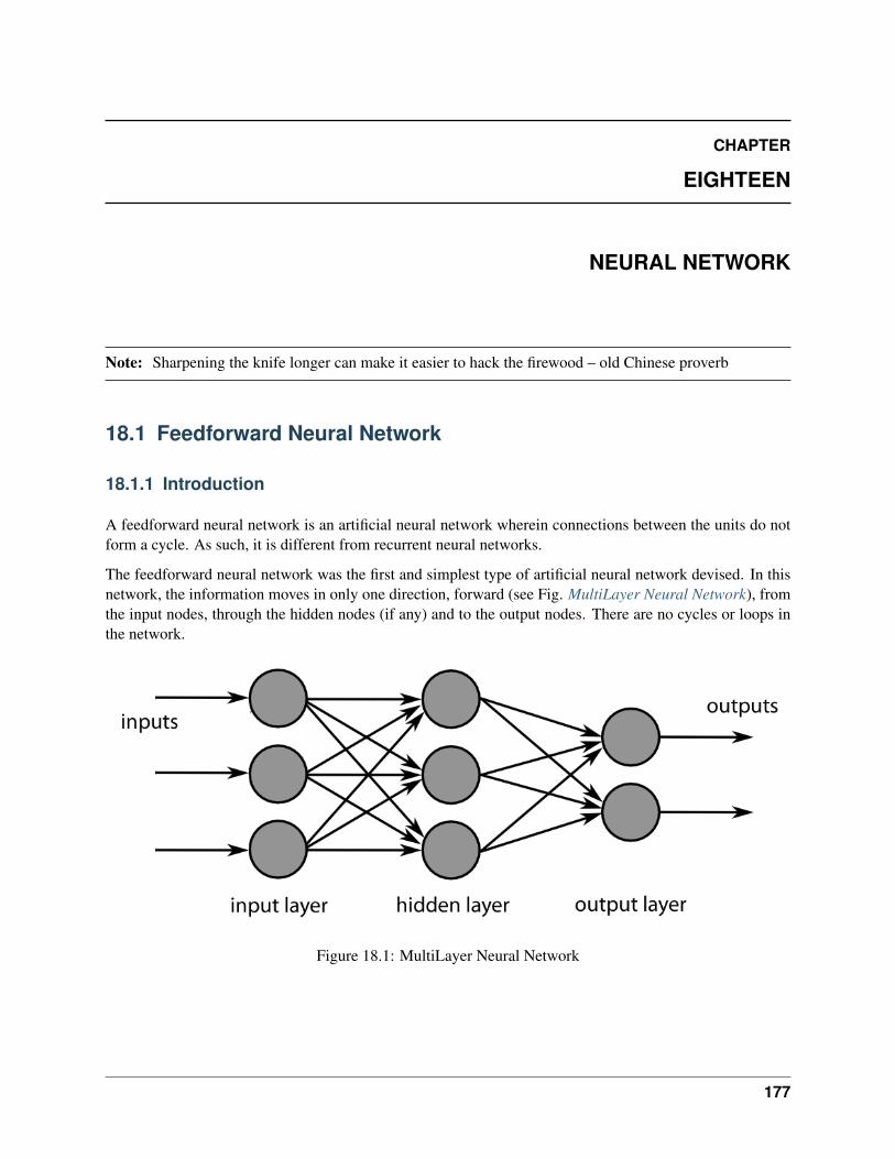
CHAPTER
EIGHTEEN
NEURAL NETWORK
Note: Sharpening the knife longer can make it easier to hack the firewood – old Chinese proverb
18.1 Feedforward Neural Network
18.1.1 Introduction
A feedforward neural network is an artificial neural network wherein connections between the units do notform a cycle. As such, it is different from recurrent neural networks.
The feedforward neural network was the first and simplest type of artificial neural network devised. In thisnetwork, the information moves in only one direction, forward (see Fig. MultiLayer Neural Network), fromthe input nodes, through the hidden nodes (if any) and to the output nodes. There are no cycles or loops inthe network.
Figure 18.1: MultiLayer Neural Network
177
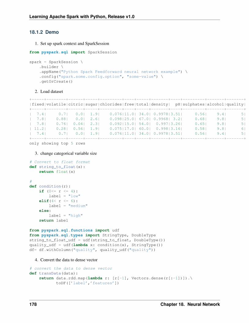
Learning Apache Spark with Python, Release v1.0
18.1.2 Demo
1. Set up spark context and SparkSession
from pyspark.sql import SparkSession
spark = SparkSession \.builder \.appName("Python Spark Feedforward neural network example") \.config("spark.some.config.option", "some-value") \.getOrCreate()
2. Load dataset
+-----+--------+------+-----+---------+----+-----+-------+----+---------+-------+-------+|fixed|volatile|citric|sugar|chlorides|free|total|density| pH|sulphates|alcohol|quality|+-----+--------+------+-----+---------+----+-----+-------+----+---------+-------+-------+| 7.4| 0.7| 0.0| 1.9| 0.076|11.0| 34.0| 0.9978|3.51| 0.56| 9.4| 5|| 7.8| 0.88| 0.0| 2.6| 0.098|25.0| 67.0| 0.9968| 3.2| 0.68| 9.8| 5|| 7.8| 0.76| 0.04| 2.3| 0.092|15.0| 54.0| 0.997|3.26| 0.65| 9.8| 5|| 11.2| 0.28| 0.56| 1.9| 0.075|17.0| 60.0| 0.998|3.16| 0.58| 9.8| 6|| 7.4| 0.7| 0.0| 1.9| 0.076|11.0| 34.0| 0.9978|3.51| 0.56| 9.4| 5|+-----+--------+------+-----+---------+----+-----+-------+----+---------+-------+-------+only showing top 5 rows
3. change categorical variable size
# Convert to float formatdef string_to_float(x):
return float(x)
#def condition(r):
if (0<= r <= 4):label = "low"
elif(4< r <= 6):label = "medium"
else:label = "high"
return label
from pyspark.sql.functions import udffrom pyspark.sql.types import StringType, DoubleTypestring_to_float_udf = udf(string_to_float, DoubleType())quality_udf = udf(lambda x: condition(x), StringType())df= df.withColumn("quality", quality_udf("quality"))
4. Convert the data to dense vector
# convert the data to dense vectordef transData(data):
return data.rdd.map(lambda r: [r[-1], Vectors.dense(r[:-1])]).\toDF([’label’,’features’])
178 Chapter 18. Neural Network
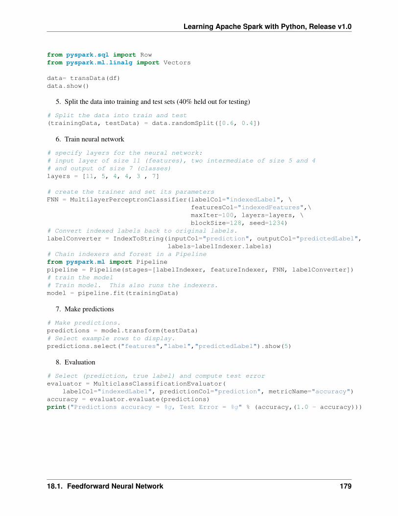
Learning Apache Spark with Python, Release v1.0
from pyspark.sql import Rowfrom pyspark.ml.linalg import Vectors
data= transData(df)data.show()
5. Split the data into training and test sets (40% held out for testing)
# Split the data into train and test(trainingData, testData) = data.randomSplit([0.6, 0.4])
6. Train neural network
# specify layers for the neural network:# input layer of size 11 (features), two intermediate of size 5 and 4# and output of size 7 (classes)layers = [11, 5, 4, 4, 3 , 7]
# create the trainer and set its parametersFNN = MultilayerPerceptronClassifier(labelCol="indexedLabel", \
featuresCol="indexedFeatures",\maxIter=100, layers=layers, \blockSize=128, seed=1234)
# Convert indexed labels back to original labels.labelConverter = IndexToString(inputCol="prediction", outputCol="predictedLabel",
labels=labelIndexer.labels)# Chain indexers and forest in a Pipelinefrom pyspark.ml import Pipelinepipeline = Pipeline(stages=[labelIndexer, featureIndexer, FNN, labelConverter])# train the model# Train model. This also runs the indexers.model = pipeline.fit(trainingData)
7. Make predictions
# Make predictions.predictions = model.transform(testData)# Select example rows to display.predictions.select("features","label","predictedLabel").show(5)
8. Evaluation
# Select (prediction, true label) and compute test errorevaluator = MulticlassClassificationEvaluator(
labelCol="indexedLabel", predictionCol="prediction", metricName="accuracy")accuracy = evaluator.evaluate(predictions)print("Predictions accuracy = %g, Test Error = %g" % (accuracy,(1.0 - accuracy)))
18.1. Feedforward Neural Network 179

Learning Apache Spark with Python, Release v1.0
180 Chapter 18. Neural Network
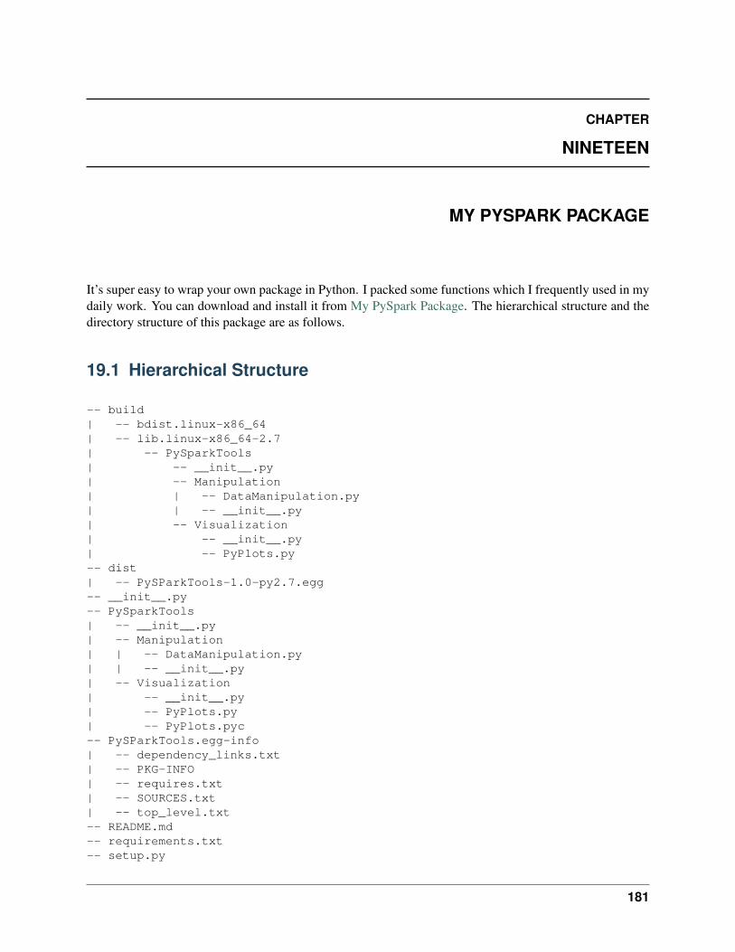
CHAPTER
NINETEEN
MY PYSPARK PACKAGE
It’s super easy to wrap your own package in Python. I packed some functions which I frequently used in mydaily work. You can download and install it from My PySpark Package. The hierarchical structure and thedirectory structure of this package are as follows.
19.1 Hierarchical Structure
-- build| -- bdist.linux-x86_64| -- lib.linux-x86_64-2.7| -- PySparkTools| -- __init__.py| -- Manipulation| | -- DataManipulation.py| | -- __init__.py| -- Visualization| -- __init__.py| -- PyPlots.py-- dist| -- PySParkTools-1.0-py2.7.egg-- __init__.py-- PySparkTools| -- __init__.py| -- Manipulation| | -- DataManipulation.py| | -- __init__.py| -- Visualization| -- __init__.py| -- PyPlots.py| -- PyPlots.pyc-- PySParkTools.egg-info| -- dependency_links.txt| -- PKG-INFO| -- requires.txt| -- SOURCES.txt| -- top_level.txt-- README.md-- requirements.txt-- setup.py
181
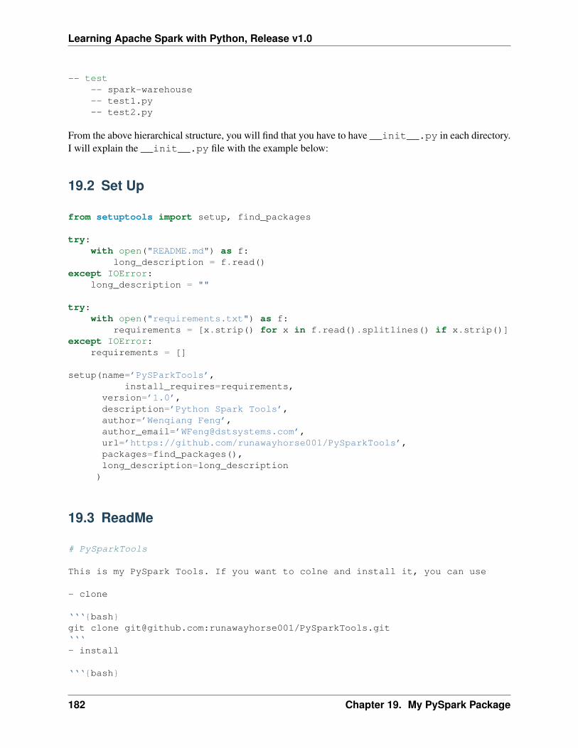
Learning Apache Spark with Python, Release v1.0
-- test-- spark-warehouse-- test1.py-- test2.py
From the above hierarchical structure, you will find that you have to have __init__.py in each directory.I will explain the __init__.py file with the example below:
19.2 Set Up
from setuptools import setup, find_packages
try:with open("README.md") as f:
long_description = f.read()except IOError:
long_description = ""
try:with open("requirements.txt") as f:
requirements = [x.strip() for x in f.read().splitlines() if x.strip()]except IOError:
requirements = []
setup(name=’PySParkTools’,install_requires=requirements,
version=’1.0’,description=’Python Spark Tools’,author=’Wenqiang Feng’,author_email=’[email protected]’,url=’https://github.com/runawayhorse001/PySparkTools’,packages=find_packages(),long_description=long_description)
19.3 ReadMe
# PySparkTools
This is my PySpark Tools. If you want to colne and install it, you can use
- clone
‘‘‘{bash}git clone [email protected]:runawayhorse001/PySparkTools.git‘‘‘- install
‘‘‘{bash}
182 Chapter 19. My PySpark Package
Learning Apache Spark with Python, Release v1.0
cd PySparkToolspip install -r requirements.txtpython setup.py install‘‘‘
- test
‘‘‘{bash}cd PySparkTools/testpython test1.py‘‘‘
19.3. ReadMe 183
Learning Apache Spark with Python, Release v1.0
184 Chapter 19. My PySpark Package

CHAPTER
TWENTY
MAIN REFERENCE
185

Learning Apache Spark with Python, Release v1.0
186 Chapter 20. Main Reference
BIBLIOGRAPHY
[Bird2009] 19. Bird, E. Klein, and E. Loper. Natural language processing with Python: analyzing textwith the natural language toolkit. O’Reilly Media, Inc., 2009.
[Feng2017] 23. Feng and M. Chen. Learning Apache Spark, Github 2017.
[Karau2015] 8. Karau, A. Konwinski, P. Wendell and M. Zaharia. Learning Spark: Lightning-Fast BigData Analysis. O’Reilly Media, Inc., 2015
[Kirillov2016] Anton Kirillov. Apache Spark: core concepts, architecture and internals.http://datastrophic.io/core-concepts-architecture-and-internals-of-apache-spark/
187

Learning Apache Spark with Python, Release v1.0
188 Bibliography
INDEX
CConfigure Spark on Mac and Ubuntu, 14
RRun on Databricks Community Cloud, 9
SSet up Spark on Cloud, 19
189


![[@NaukriEngineering] Apache Spark](https://img.dokumen.tips/doc/110x75/588304451a28abe70d8b6157/naukriengineering-apache-spark.jpg)