Learning accurate and concise na¨ıve Bayes classiﬁers …honavar/Papers/KIS-Jun.pdfLearning accurate and concise na¨ıve Bayes classiﬁers from attribute value taxonomies and

Knowl Inf Syst (2005)DOI 10.1007/s10115-005-0211-z

Knowledge andInformation Systems

RESEARCH ARTICLE

J. Zhang · D.-K. Kang ·A. Silvescu · V. Honavar

Learning accurate and concise naıve Bayesclassifiers from attribute value taxonomiesand data

Received: 1 November 2004 / Revised: 25 January 2005 / Accepted: 19 February 2005 /Published online: 24 June 2005C© Springer-Verlag 2005

Abstract In many application domains, there is a need for learning algorithmsthat can effectively exploit attribute value taxonomies (AVT)—hierarchical group-ings of attribute values—to learn compact, comprehensible and accurate classifiersfrom data—including data that are partially specified. This paper describes AVT-NBL, a natural generalization of the naıve Bayes learner (NBL), for learning clas-sifiers from AVT and data. Our experimental results show that AVT-NBL is ableto generate classifiers that are substantially more compact and more accurate thanthose produced by NBL on a broad range of data sets with different percentages ofpartially specified values. We also show that AVT-NBL is more efficient in its useof training data: AVT-NBL produces classifiers that outperform those produced byNBL using substantially fewer training examples.

Keywords Attribute value taxonomies · AVT-based naıve Bayes learner ·Partially specified data

1 Introduction

Synthesis of accurate and compact pattern classifiers from data is one of the ma-jor applications of data mining. In a typical inductive learning scenario, instances

This paper is an extended version of a paper published in the 4th IEEE International Conferenceon Data Mining, 2004.

J. Zhang(B) · D.-K. Kang · A. SilvescuDepartment of Computer Science, Artificial Intelligence Research Laboratory, ComputationalIntelligence, Learning, and Discovery Program, Iowa State University, Ames, Iowa 50011-1040,USA E-mail: [email protected]

V. HonavarDepartment of Computer Science, Artificial Intelligence Research Laboratory; ComputationalIntelligence, Learning, and Discovery Program; Bioinformatics and Computational Biology Pro-gram, Iowa State University, Ames, Iowa 50011-1040, USA

J. Zhang et al.

to be classified are represented as ordered tuples of attribute values. However,attribute values can be grouped together to reflect assumed or actual similaritiesamong the values in a domain of interest or in the context of a specific application.Such a hierarchical grouping of attribute values yields an attribute value taxonomy(AVT). Such AVT are quite common in biological sciences. For example, the GeneOntology Consortium is developing hierarchical taxonomies for describing manyaspects of macromolecular sequence, structure and function [5]. Undercoffer etal. have developed a hierarchical taxonomy that captures the features that are ob-servable or measurable by the target of an attack or by a system of sensors actingon behalf of the target [41]. Several ontologies being developed as part of theSemantic Web-related efforts [7] also capture hierarchical groupings of attributevalues. Kohavi and Provost have noted the need to be able to incorporate back-ground knowledge in the form of hierarchies over data attributes in e-commerceapplications of data mining [25, 26]. Against this background, algorithms forlearning from AVT and data are of significant practical interest for severalreasons:

(a) An important goal of machine learning is to discover comprehensible, yetaccurate and robust, classifiers [34]. The availability of AVT presents the op-portunity to learn classification rules that are expressed in terms of abstractattribute values leading to simpler, accurate and easier-to-comprehend rulesthat are expressed using familiar hierarchically related concepts [25, 44].

(b) Exploiting AVT in learning classifiers can potentially perform regulariza-tion to minimize overfitting when learning from relatively small data sets. Acommon approach used by statisticians when estimating from small samplesinvolves shrinkage [29] to estimate the relevant statistics with adequate confi-dence. Learning algorithms that exploit AVT can potentially perform shrink-age automatically, thereby yielding robust classifiers and minimizing over-fitting.

(c) The presence of explicitly defined AVT allows specification of data at differ-ent levels of precision, giving rise to partially specified instances [45]. Theattribute value of a particular attribute can be specified at different levels ofprecision in different instances. For example, the medical diagnostic test re-sults given by different institutions are presented at different levels of preci-sion. Partially specified data are unavoidable in knowledge acquisition scenar-ios that call for integration of information from semantically heterogeneousinformation sources [10]. Semantic differences between information sourcesarise as a direct consequence of differences in ontological commitments [7].Hence, algorithms for learning classifiers from AVT and partially specifieddata are of great interest.

Against this background, this paper introduces AVT-NBL, an AVT-based gen-eralization of the standard algorithm for learning naıve Bayes classifiers from par-tially specified data. The rest of the paper is organized as follows: Sect. 2 formal-izes the notions on learning classifiers with AVT taxonomies; Sect. 3 presentsthe AVT-NBL algorithm; Sect. 4 discusses briefly on alternative approaches;Sect. 5 describes our experimental results and Sect. 6 concludes with summary anddiscussion.

Learning accurate and concise naıve Bayes classifiers from AVT and data

2 Preliminaries

In what follows, we formally define AVT and its induced instance space. We in-troduce the notion of partially specified instances and formalize the problem oflearning from AVT and data.

2.1 Attribute value taxonomies

Let A = {A1, A2, . . . , AN } be an ordered set of nominal attributes and letdom(Ai ) denote the set of values (the domain) of attribute Ai . We formally de-fine attribute value taxonomy (AVT) as follows:

Definition 2.1 (Attribute Value Taxonomy) Attribute value taxonomy Ti for at-tribute Ai is a Tree-structured concept hierarchy in the form of a partially orderset (dom(Ai ), ≺), where dom(Ai ) is a finite set that enumerates all attribute val-ues in Ai and ≺ is the partial order that specifies a relationships among attributevalues in dom(Ai ). Collectively, T = {T1, T2, . . . , TN } represents the ordered setof attribute value taxonomies associated with attributes A1, A2, . . . , AN .

Let Nodes(Ti ) represent the set of all values in Ti , and Root(Ti ) standfor the root of Ti . The set of leaves of the tree, Leaves(Ti ), corresponds tothe set of primitive values of attribute Ai . The internal nodes of the tree (i.e.Nodes(Ti )−Leaves(Ti )) correspond to abstract values of attribute Ai . Each arcof the tree corresponds to a relationship over attribute values in the AVT. Thus, anAVT defines an abstraction hierarchy over values of an attribute.

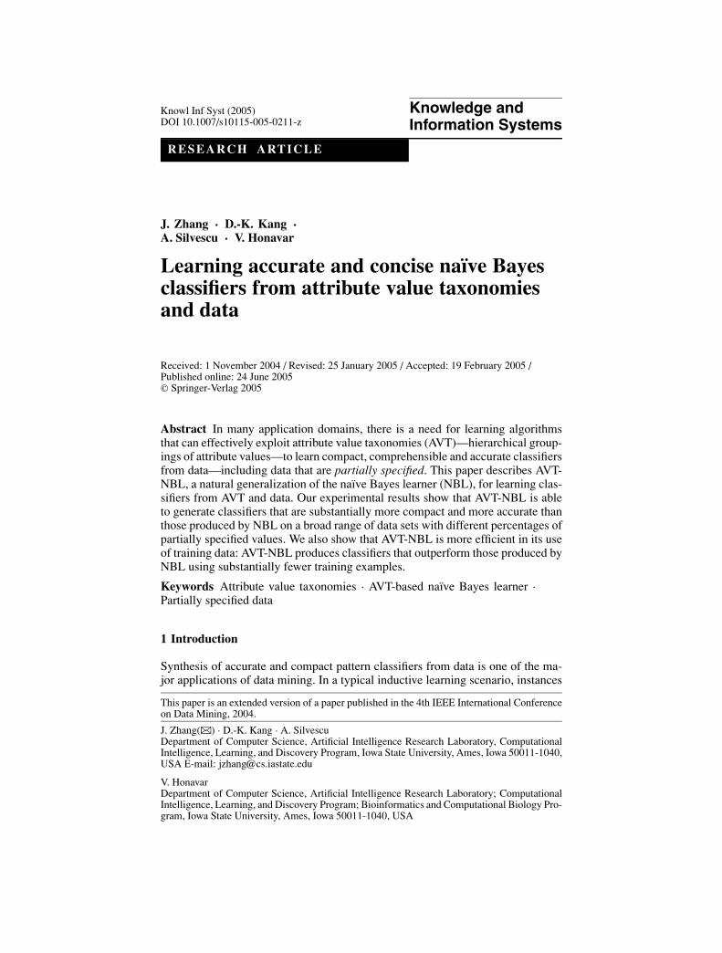
For example, Fig. 1 shows two attributes with corresponding AVTs for de-scribing students in terms of their student status and work status. With regard tothe AVT associated with student status, Sophomore is a primitive value while Un-dergraduate is an abstract value. Undergraduate is an abstraction of Sophomore,whereas Sophomore is a further specification of Undergraduate. We can similarlydefine AVT over ordered attributes as well as intervals defined over numericalattributes.

After [21], we define a cut γi for Ti as follows:

Definition 2.2 (Cut) A cut γi is a subset of elements in Nodes(Ti ) satisfying thefollowing two properties: (1) For any leaf m ∈ Leaves(Ti ), either m ∈ γi or m

Student Status Work Status

Freshman

Undergraduate Graduate

JuniorSophomore

Senior

Master Ph.D

On-Campus Off-Campus

TA RA AA

Government Private

Federal State

Com Org

Fig. 1 Two attribute value taxonomies on student status and work status.

J. Zhang et al.

is a descendant of an element n ∈ γi ; and (2) for any two nodes f, g ∈ γi , f isneither a descendant nor an ancestor of g.

The set of abstract attribute values at any given cut of Ti form a partition of theset of values at a lower level cut and also induce a partition of all primitive valuesof Ai . For example, in Fig. 1, the cut {Undergraduate, Graduate} defines a parti-tion over all the primitive values {Freshman, Sophomore, Junior, Senior, Master,PhD} in the student status attribute, and the cut {On-Campus, Off-Campus} de-fines a partition over its lower level cut {On-Campus, Government, Private} in thework status attribute.

For attribute Ai , we denote �i to be the set of all valid cuts in Ti . We denote� = ×N

i=1 �i to be the Cartesian product of the cuts through the individual AVTs.Hence, � = {γ1, γ2, . . . , γN } defines a global cut through T = {T1, T2, . . . , TN },where each γi ∈ �i and � ∈ �.

Definition 2.3 (Cut Refinement) We say that a cut γi is a refinement of a cut γiif γi is obtained by replacing at least one attribute value v ∈ γi by its descendantsψ(v, Ti ). Conversely, γi is an abstraction of γi . We say that a global cut � is arefinement of a global cut � if at least one cut in � is a refinement of a cut in �.Conversely, the global cut � is an abstraction of the global cut �.

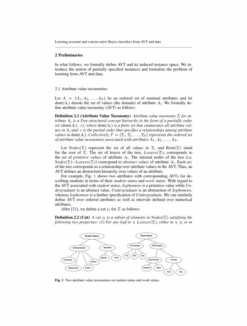
As an example, Fig. 2 illustrates a demonstrative cut refinement process basedon the AVTs shown in Fig. 1. The cut γ1 = {Undergraduate, Graduate} inthe student status attribute has been refined to γ1 = {Undergraduate, Master,PhD} by replacing Graduate with its two children, Master, PhD. Therefore, �= {Undergraduate, Master, PhD, On-Campus, Off-Campus} is a cut refinementof � = {Undergraduate, Graduate, On-Campus, Off-Campus}.

2.2 AVT-induced abstract-instance space

A classifier is built on a set of labeled training instances. The original instancespace I without AVTs is an instance space defined over the domains of all at-tributes. We can formally define AVT-induced instance space as follows:

Student Status Work Status

Freshman


JuniorSophomore

Senior

Master Ph.D

On-Campus Off-Campus

TA RA AA

Government Private

Federal State

Com Org 11

ˆγ γ

Γ

Γ

ˆ

Fig. 2 Cut refinement. The cut γ1 = {Undergraduate, Graduate} in the student status at-tribute has been refined to γ1 = {Undergraduate, Master, PhD}, such that the global cut � ={Undergraduate, Graduate, On-Campus, Off-Campus} has been refined to � = {Undergraduate,Master, PhD, On-Campus, Off-Campus}.


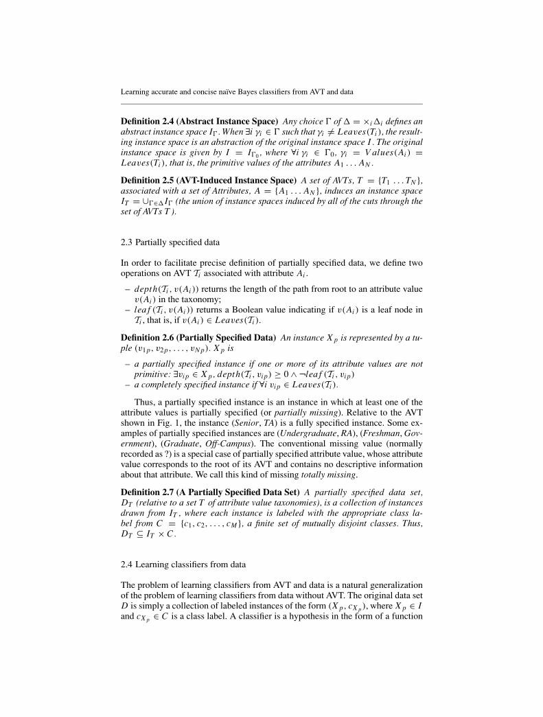
Definition 2.4 (Abstract Instance Space) Any choice � of � = ×i�i defines anabstract instance space I� . When ∃i γi ∈ � such that γi �= Leaves(Ti ), the result-ing instance space is an abstraction of the original instance space I . The originalinstance space is given by I = I�0 , where ∀i γi ∈ �0, γi = V alues(Ai ) =Leaves(Ti ), that is, the primitive values of the attributes A1 . . . AN .

Definition 2.5 (AVT-Induced Instance Space) A set of AVTs, T = {T1 . . . TN },associated with a set of Attributes, A = {A1 . . . AN }, induces an instance spaceIT = ∪�∈� I� (the union of instance spaces induced by all of the cuts through theset of AVTs T ).

2.3 Partially specified data

In order to facilitate precise definition of partially specified data, we define twooperations on AVT Ti associated with attribute Ai .

– depth(Ti , v(Ai )) returns the length of the path from root to an attribute valuev(Ai ) in the taxonomy;

– lea f (Ti , v(Ai )) returns a Boolean value indicating if v(Ai ) is a leaf node inTi , that is, if v(Ai ) ∈ Leaves(Ti ).

Definition 2.6 (Partially Specified Data) An instance X p is represented by a tu-ple (v1p, v2p, . . . , vN p). X p is

– a partially specified instance if one or more of its attribute values are notprimitive: ∃vi p ∈ X p, depth(Ti , vi p) ≥ 0 ∧ ¬lea f (Ti , vi p)

– a completely specified instance if ∀i vi p ∈ Leaves(Ti ).

Thus, a partially specified instance is an instance in which at least one of theattribute values is partially specified (or partially missing). Relative to the AVTshown in Fig. 1, the instance (Senior, TA) is a fully specified instance. Some ex-amples of partially specified instances are (Undergraduate, RA), (Freshman, Gov-ernment), (Graduate, Off-Campus). The conventional missing value (normallyrecorded as ?) is a special case of partially specified attribute value, whose attributevalue corresponds to the root of its AVT and contains no descriptive informationabout that attribute. We call this kind of missing totally missing.

Definition 2.7 (A Partially Specified Data Set) A partially specified data set,DT (relative to a set T of attribute value taxonomies), is a collection of instancesdrawn from IT , where each instance is labeled with the appropriate class la-bel from C = {c1, c2, . . . , cM }, a finite set of mutually disjoint classes. Thus,DT ⊆ IT × C.

2.4 Learning classifiers from data

The problem of learning classifiers from AVT and data is a natural generalizationof the problem of learning classifiers from data without AVT. The original data setD is simply a collection of labeled instances of the form (X p, cX p ), where X p ∈ Iand cX p ∈ C is a class label. A classifier is a hypothesis in the form of a function

J. Zhang et al.

h : I → C , whose domain is the instance space I and whose range is the set ofclasses C . An hypothesis space H is a set of hypotheses that can be represented insome hypothesis language or by a parameterised family of functions (e.g. decisiontrees, naıve Bayes classifiers, SVM, etc.). The task of learning classifiers from theoriginal data set D entails identifying a hypothesis h ∈ H that satisfies somecriteria (e.g. a hypothesis that is most likely given the training data D).

The problem of learning classifiers from AVT and data can be stated as fol-lows:

Definition 2.8 (Learning Classifiers from AVT and Data) Given a user-supplied set of AVTs, T , and a data set, DT , of (possibly) partially specifiedlabeled instances, construct a classifier hT : IT → C for assigning appropriateclass labels to each instance in the instance space IT .

Of special interest are the cases in which the resulting hypothesis space HThas structure that makes it possible to search it efficiently for a hypothesis that isboth concise as well as accurate.

3 AVT-based naıve Bayes learner

3.1 Naıve Bayes learner (NBL)

Naıve Bayes classifier is a simple and yet effective classifier that has competitiveperformance with other more sophisticated classifiers [18]. Naıve Bayes classifieroperates under the assumption that each attribute is independent of others giventhe class. Thus, the joint probability given a class can be written as the productof individual class conditional probabilities for each attribute. The Bayesian ap-proach to classifying an instance X p = (v1p, v2p, . . . , vN p) is to assign it themost probable class cMAP(X p):

cMAP(X p) = argmaxc j ∈C

P(v1p, v2p, . . . , vN p|c j )p(c j )

= argmaxc j ∈C

p(c j )∏

i

P(vi p|c j ).

The task of the naıve Bayes Learner (NBL) is to estimate ∀c j ∈ C and∀vik ∈ dom(Ai ), relevant class probabilities, p(c j ), and the class conditionalprobabilities, P(vik |c j ), from training data, D. These probabilities, which com-pletely specify a naıve Bayes classifier, can be estimated from a training set,D, using standard probability estimation methods [31] based on relative fre-quency counts of the corresponding classes and attribute value and class label co-occurrences observed in D. We denote σi (vk |c j ) as the frequency count of valuevk of attribute Ai given class label c j and σ(c j ) as the frequency count of classlabel c j in a training set D. Hence, these relative frequency counts completelysummarize the information needed for constructing a naıve Bayes classifier fromD, and they constitute sufficient statistics for naıve Bayes learner [9, 10].


3.2 AVT-NBL

We now introduce AVT-NBL, an algorithm for learning naıve Bayes classifiersfrom AVT and data. Given an ordered set of AVTs, T = {T1, T2, . . . , TN }, corre-sponding to the attributes A = {A1, A2, . . . , AN } and a data set D = {(X p, cX p )}of labeled examples of the form (X p, cX p ), where X p ∈ IT is a partially or fullyspecified instance and cX p ∈ C is the corresponding class label, the task of AVT-NBL is to construct a naıve Bayes classifier for assigning X p to its most probableclass, cMAP(X p). As in the case of NBL, we assume that each attribute is indepen-dent of the other attributes given the class.

Let � = {γ1, γ2, . . . , γN } be a global cut, where γi stands for a cut through Ti .A naıve Bayes classifier defined on the instance space I� is completely specifiedby a set of class conditional probabilities for each value of each attribute. Supposewe denote the table of class conditional probabilities associated with values in γiby C PT (γi ). Then the naıve Bayes classifier defined over the instance space I� isspecified by h(�) = {C PT (γ1), C PT (γ2), . . . , C PT (γN )}.

If each cut, γi ∈ �0 is chosen to correspond to the primitive values of therespective attribute, i.e. ∀i γi = Leaves(Ti ). h(�0) is simply the standard naıveBayes classifier based on the attributes A1, A2, . . . , AN . If each cut γi ∈ � ischosen to pass through the root of each AVT, i.e. ∀i γi = {Root(Ti )}, h(�) simplyassigns each instance to the class that is a priori most probable.

AVT-NBL starts with the naıve Bayes classifier that is based on the most ab-stract value of each attribute (the most general hypothesis in HT ) and successivelyrefines the classifier (hypothesis) using a criterion that is designed to trade offbetween the accuracy of classification and the complexity of the resulting naıveBayes classifier. Successive refinements of � correspond to a partial ordering ofnaıve Bayes classifiers based on the structure of the AVTs in T .

For example, in Fig. 2, � is a cut refinement of �, and hence corresponding hy-pothesis h(�) is a refinement of h(�). Relative to the two cuts, Table 1 shows theconditional probability tables that we need to compute during learning for h(�)

and h(�), respectively (assuming C = {+, −} as two possible class labels). Fromthe class conditional probability table, we can count the number of class condi-tional probabilities needed to specify the corresponding naıve Bayes classifier. Asshown in Table 1, the total number of class conditional probabilities for h(�) andh(�) are 8 and 10, respectively.

3.2.1 Class conditional frequency counts

Given an attribute value taxonomy Ti for attribute Ai , we can define a tree of classconditional frequency counts CC FC(Ti ) such that there is a one-to-one corre-spondence between the nodes of the AVT Ti and the nodes of the correspondingCC FC(Ti ). It follows that the class conditional frequency counts associated witha nonleaf node of CC FC(Ti ) should correspond to the aggregation of the corre-sponding class conditional frequency counts associated with its children. Becauseeach cut through an AVT Ti corresponds to a partition of the set of possible val-ues in Nodes(Ti ) of the attribute Ai , the corresponding cut γi through CC FC(Ti )specifies a valid class conditional probability table C PT (γi ) for the attribute Ai .

J. Zhang et al.

Table 1 Conditional probability tables. This table shows the entries of conditional probabilitytables associated with two global cut � and � shown in Fig. 2 (assuming C = +, −).

Value Pr(+) Pr(−)

CPT for h(�)Undergraduate P(Undergraduate|+) P(Undergraduate|−)Graduate P(Graduate|+) P(Graduate|−)On-Campus P(On-Campus|+) P(On-Campus|−)Off-Campus P(Off-Campus|+) P(Off-Campus|−)

CPT for h( �)Undergraduate P(Undergraduate|+) P(Undergraduate|−)Master P(Master|+) P(Master|−)PhD P(Ph.D.|+) P(PhD|−)On-Campus P(On-Campus|+) P(On-Campus|−)Off-Campus P(Off-Campus|+) P(Off-Campus|−)

In the case of numerical attributes, AVTs are defined over intervals based onobserved values for the attribute in the data set. Each cut through the AVT corre-sponds to a partition of the numerical attribute into a set of intervals. We calculatethe class conditional probabilities for each interval. As in the case of nominal at-tributes, we define a tree of class conditional frequency counts CC FC(Ti ) foreach numerical attribute Ai . CC FC(Ti ) is used to calculate the conditional prob-ability table C PT (γi ) corresponding to a cut γi .

When all of the instances in the data set D are fully specified, estimation ofCC FC(Ti ) for each attribute is straightforward: we simply estimate the class con-ditional frequency counts associated with each of the primitive values of Ai fromthe data set D and use them recursively to compute the class conditional frequencycounts associated with the nonleaf nodes of CC FC(Ti ).

When some of the data are partially specified, we can use a two-step processfor computing CC FC(Ti ): First we make an upward pass aggregating the classconditional frequency counts based on the specified attribute values in the data set.Then we propagate the counts associated with partially specified attribute valuesdown through the tree, augmenting the counts at lower levels according to thedistribution of values along the branches based on the subset of the data for whichthe corresponding values are fully specified1.

Let σi (v|c j ) be the frequency count of value v of attribute Ai given class labelc j in a training set D and pi (v|c j ) the estimated class conditional probability ofvalue v of attribute Ai given class label c j in a training set D. Let π(v, Ti ) bethe set of all children (direct descendants) of a node with value v in Ti ; �(v, Ti )the list of ancestors, including the root, for v in Ti . The procedure of computingCC FC(Ti ) is shown below.

Algorithm 3.1 Calculating class conditional frequency counts.

Input: Training data D and T1, T2, . . . , TN .

1 This procedure can be seen as a special case of EM (expectation maximization) algorithm[15] to estimate sufficient statistics for CC FC(Ti ).


Output: CC FC(T1), CC FC(T2), . . . , CC FC(TN ).

Step 1: Calculate frequency counts σi (v|c j ) for each node v in Ti usingthe class conditional frequency counts associated with the specified valuesof attribute Ai in training set D.Step 2: For each attribute value v in Ti that received nonzero counts as aresult of step 1, aggregate the counts upward from each such node v to itsancestors, �(v, Ti ): σi (w|c j )w∈�(v,Ti ) ← σi (w|c j ) + σi (v|c j ).Step 3: Starting from the root, recursively propagate the counts corre-sponding to partially specified instances at each node v downward ac-cording to the observed distribution among its children to obtain updatedcounts for each child ul ∈ π(v, Ti ):

σi (ul |c j ) =

(σi (v|c j )

|π(v,Ti )|)

If∑|π(v,Ti )|

k=1 σi (uk |c j )=0,

σi (ul |c j )

(1 + σi (v|c j ) − ∑|π(v,Ti )|

k=1 σi (uk |c j )∑|π(v,Ti )|k=1 σi (uk |c j )

)Otherwise.

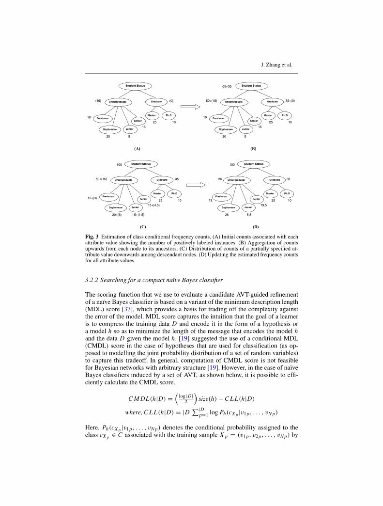
We use a simple example to illustrate the estimation of class conditional fre-quency counts when some of the instances are partially specified. On the AVTfor student status shown in Fig. 3(A), we mark each attribute value with a countshowing the total number of positively labeled (+) instances having that specificvalue. First, we aggregate the counts upward from each node to its ancestors. Forexample, in Fig. 3(B), the four counts 10, 20, 5, 15 on primitive attribute valuesFreshman, Sophomore, Junior, and Senior add up to 50 as the count for Under-graduate. Because we also have 15 instances that are partially specified with thevalue Undergraduate, the two counts (15 and 50) aggregate again toward the root.Next, we distribute the counts of a partially specified attribute value downward ac-cording to the distributions of values among their descendant nodes. For example,15, the count of partially specified attribute value Undergraduate, is propagateddown into fractional counts 3, 6, 1.5, 4.5 for Freshman, Sophomore, Junior andSenior (see Fig. 3(C) for values in parentheses). Finally, we update the estimatedfrequency counts for all attribute values as shown in Fig. 3(D).

Now that we have estimated the class conditional frequency counts for all at-tribute value taxonomies, we can calculate the conditional probability table withregard to any global cut �. Let � = {γ1, . . . , γN } be a global cut, where γistands for a cut through CC FC(Ti ). The estimated conditional probability ta-ble C PT (γi ) associated with the cut γi can be calculated from CC FC(Ti ) usingLaplace estimates [31, 24].

pi (v|c j )v∈γi ← 1/|D| + σi (v|c j )

|γi |/|D| +∑

u∈γi

σi (u|c j )

Recall that the naıve Bayes classifier h(�) based on a chosen global cut � iscompletely specified by the conditional probability tables associated with the cutsin �: h(�) = {C PT (γ1), . . . , C PT (γN )}.

J. Zhang et al.

(A)

10

20 5

15

Student Status

Freshman


JuniorSophomore

Senior

Master Ph.D

(15)

25 10

(0)

(B)

10

20 5

15

Student Status

Freshman


JuniorSophomore

Senior

Master Ph.D

25 10

65+35

50+(15) 35+(0)

(C)

10+(3)

20+(6) 5+(1.5)

15+(4.5)

Student Status

Freshman


JuniorSophomore

Senior

Master Ph.D

25 10

50+(15) 35

100

(D)

13

26 6.5

19.5

Student Status

Freshman


JuniorSophomore

Senior

Master Ph.D

25 10

65 35

100

Fig. 3 Estimation of class conditional frequency counts. (A) Initial counts associated with eachattribute value showing the number of positively labeled instances. (B) Aggregation of countsupwards from each node to its ancestors. (C) Distribution of counts of a partially specified at-tribute value downwards among descendant nodes. (D) Updating the estimated frequency countsfor all attribute values.

3.2.2 Searching for a compact naıve Bayes classifier

The scoring function that we use to evaluate a candidate AVT-guided refinementof a naıve Bayes classifier is based on a variant of the minimum description length(MDL) score [37], which provides a basis for trading off the complexity againstthe error of the model. MDL score captures the intuition that the goal of a learneris to compress the training data D and encode it in the form of a hypothesis ora model h so as to minimize the length of the message that encodes the model hand the data D given the model h. [19] suggested the use of a conditional MDL(CMDL) score in the case of hypotheses that are used for classification (as op-posed to modelling the joint probability distribution of a set of random variables)to capture this tradeoff. In general, computation of CMDL score is not feasiblefor Bayesian networks with arbitrary structure [19]. However, in the case of naıveBayes classifiers induced by a set of AVT, as shown below, it is possible to effi-ciently calculate the CMDL score.

C M DL(h|D) =(

log |D|2

)size(h) − C L L(h|D)

where, C L L(h|D) = |D|∑|D|p=1 log Ph(cX p |v1p, . . . , vN p)

Here, Ph(cX p |v1p, . . . , vN p) denotes the conditional probability assigned to theclass cX p ∈ C associated with the training sample X p = (v1p, v2p, . . . , vN p) by


the classifier h, size(h) is the number of parameters used by h, |D| the size ofthe data set, and C L L(h|D) is the conditional log likelihood of the hypothesis hgiven the data D. In the case of a naıve Bayes classifier h, size(h) corresponds tothe total number of class conditional probabilities needed to describe h. Becauseeach attribute is assumed to be independent of the others given the class in a naıveBayes classifier, we have

C L L(h|D) = |D| ∑|D|p=1 log

(P(cX p )

∏i Ph(vi p |cX p )

∑|C |j=1 P(c j )

∏i Ph(vi p |c j )

),

where P(c j ) is the prior probability of the class c j , which can be estimated fromthe observed class distribution in the data D.

It is useful to distinguish between two cases in the calculation of the con-ditional likelihood C L L(h|D) when D contains partially specified instances:(1) When a partially specified value of attribute Ai for an instance lies on the cut γthrough CC FC(Ti ) or corresponds to one of the descendants of the nodes in thecut. In this case, we can treat that instance as though it were fully specified relativeto the naıve Bayes classifier based on the cut γ of CC FC(Ti ) and use the classconditional probabilities associated with the cut γ to calculate its contribution toC L L(h|D). (2) When a partially specified value (say v) of Ai is an ancestor of asubset (say λ ) of the nodes in γ . In this case, p(v|c j ) = ∑

ui ∈λ p(ui |c j ), such thatwe can aggregate the class conditional probabilities of the nodes in λ to calculatethe contribution of the corresponding instance to C L L(h|D).

Because each attribute is assumed to be independent of others given theclass, the search for the AVT-based naıve Bayes classifier (AVT-NBC) can beperformed efficiently by optimizing the criterion independently for each attribute.This results in a hypothesis h that intuitively trades off the complexity of naıveBayes classifier (in terms of the number of parameters used to describe therelevant class conditional probabilities) against accuracy of classification. Thealgorithm terminates when none of the candidate refinements of the classifieryield statistically significant improvement in the CMDL score. The procedure isoutlined below.

Algorithm 3.2 Searching for compact AVT-based naıve Bayes classifier.

Input: Training data D and CC FC(T1), CC FC(T2), . . . , CC FC(TN ).Output: A naıve Bayes classifier trading off the complexity against theerror.

1. Initialize each γi in � = {γ1, γ2, . . . , γN } to {Root(Ti )}.2. Estimate probabilities that specify the hypothesis h(�).3. For each cut γi in � = {γ1, γ2, . . . , γN }:

A. Set δi ← γiB. Until there are no updates to γi

i. For each v ∈ δia. Generate a refinement γ v

i of γi by replacing v with π(v, Ti ), and

refine � accordingly to obtain �. Construct corresponding hy-pothesis h(�)

J. Zhang et al.

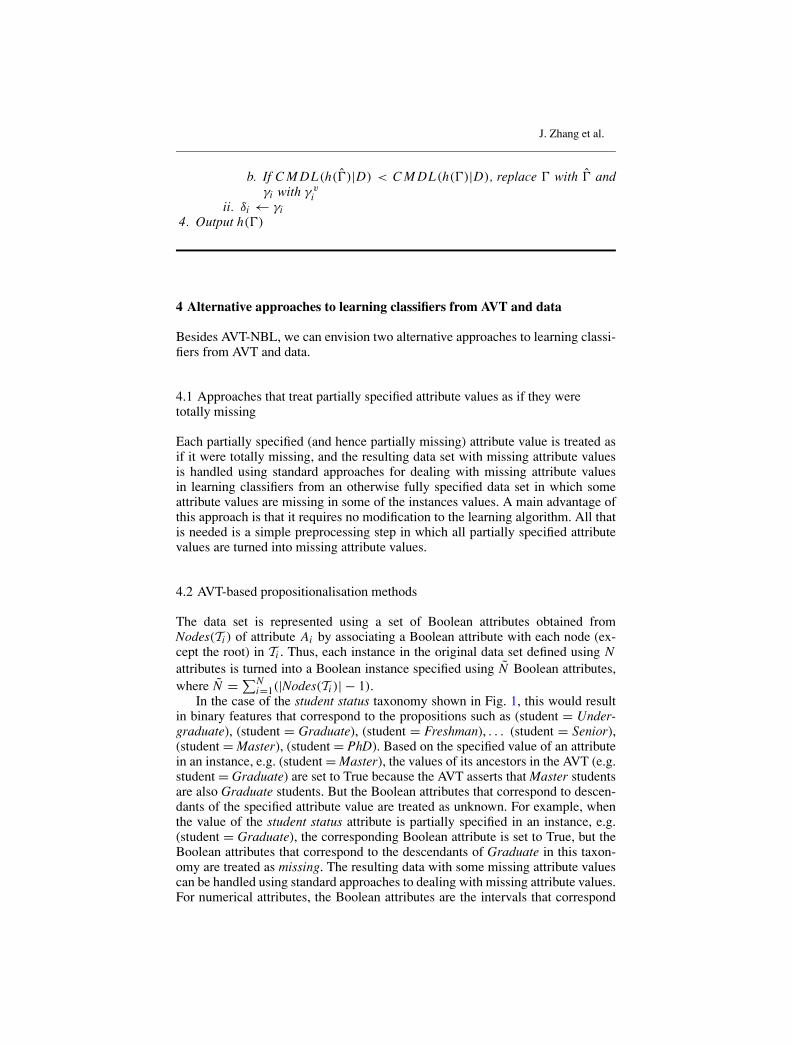
b. If C M DL(h(�)|D) < C M DL(h(�)|D), replace � with � andγi with γ v

iii. δi ← γi

4. Output h(�)

4 Alternative approaches to learning classifiers from AVT and data

Besides AVT-NBL, we can envision two alternative approaches to learning classi-fiers from AVT and data.

4.1 Approaches that treat partially specified attribute values as if they weretotally missing

Each partially specified (and hence partially missing) attribute value is treated asif it were totally missing, and the resulting data set with missing attribute valuesis handled using standard approaches for dealing with missing attribute valuesin learning classifiers from an otherwise fully specified data set in which someattribute values are missing in some of the instances values. A main advantage ofthis approach is that it requires no modification to the learning algorithm. All thatis needed is a simple preprocessing step in which all partially specified attributevalues are turned into missing attribute values.

4.2 AVT-based propositionalisation methods

The data set is represented using a set of Boolean attributes obtained fromNodes(Ti ) of attribute Ai by associating a Boolean attribute with each node (ex-cept the root) in Ti . Thus, each instance in the original data set defined using Nattributes is turned into a Boolean instance specified using N Boolean attributes,where N = ∑N

i=1(|Nodes(Ti )| − 1).In the case of the student status taxonomy shown in Fig. 1, this would result

in binary features that correspond to the propositions such as (student = Under-graduate), (student = Graduate), (student = Freshman), . . . (student = Senior),(student = Master), (student = PhD). Based on the specified value of an attributein an instance, e.g. (student = Master), the values of its ancestors in the AVT (e.g.student = Graduate) are set to True because the AVT asserts that Master studentsare also Graduate students. But the Boolean attributes that correspond to descen-dants of the specified attribute value are treated as unknown. For example, whenthe value of the student status attribute is partially specified in an instance, e.g.(student = Graduate), the corresponding Boolean attribute is set to True, but theBoolean attributes that correspond to the descendants of Graduate in this taxon-omy are treated as missing. The resulting data with some missing attribute valuescan be handled using standard approaches to dealing with missing attribute values.For numerical attributes, the Boolean attributes are the intervals that correspond


to nodes of the respective AVTs. If a numerical value falls in a certain interval, thecorresponding Boolean attribute is set to True, otherwise it is set to False. We callthe resulting algorithm—NBL applied to AVT-based propositionalized version ofthe data—Prop-NBL.

Note that the Boolean features created by the propositionalisation techniquedescribed above are not independent given the class. A Boolean attribute that cor-responds to any node in an AVT is necessarily correlated with Boolean attributesthat correspond to its descendants as well as its ancestors in the tree. For example,the Boolean attribute (student = Graduate) is correlated with (student = Master).(Indeed, it is this correlation that enables us to exploit the information providedby AVT in learning from partially specified data). Thus, a naıve Bayes classifierthat would be optimal in the maximal a posteriori sense [28] when the originalattributes student status and work status are independent given class would nolonger be optimal when the new set of Boolean attributes are used because ofstrong dependencies among the Boolean attributes derived from an AVT.

A main advantage of the AVT-based propositionalisation methods is that theyrequire no modification to the learning algorithm. However, it does require pre-processing of partially specified data using the information supplied by an AVT.The number of attributes in the transformed data set is substantially larger thanthe number of attributes in the original data set. More important, the statistical de-pendence among the Boolean attributes in the propositionalised representation ofthe original data set can degrade the performance of classifiers, e.g. naıve Bayesthat rely on independence of attributes given class. Against this background, weexperimentally compare AVT-NBL with Prop-NBL and the standard naıve Bayesalgorithm (NBL).

5 Experiments and results

5.1 Experiments

Our experiments were designed to explore the performance of AVT-NBL relativeto that of NBL and PROP-NBL.

Although partially specified data and hierarchical AVT are common in manyapplication domains, at present, there are few standard benchmark data sets of par-tially specified data and the associated AVT. We select 37 data sets from the UCIrvine Machine Learning Repository, among which 8 data sets use only nominalattributes and 29 data sets have both nominal attributes and numerical attributes.Every numerical attribute in the 29 data sets has been discretised into a maxi-mum of 10 bins. For only three of the data sets (i.e. Mushroom, Soybean, andNursery), AVTs were supplied by domain experts. For the remaining data sets,no expert-generated AVTs are readily available. Hence, the AVTs on both nom-inal and numerical attributes were generated using AVT-Learner, a hierarchicalagglomerative clustering algorithm to construct AVTs for learning [23].

The first set of experiments compares the performance of AVT-NBL, NBL,and PROP-NBL on the original data.

The second set of experiments explores the performance of the algorithms ondata sets with different percentages of totally missing and partially missing at-tribute values. Three data sets with a prespecified percentage (10%, 30% or 50%,

J. Zhang et al.

excluding the missing values in the original data set) of totally or partially miss-ing attribute values were generated by assuming that the missing values are uni-formly distributed on the nominal attributes [45]. From the original data set D,a data set Dp of partially (or totally) missing values was generated as follows:Let (nl , nl−1, . . . , n0) be the path from the fully specified primitive value nl tothe root n0 of the corresponding AVT. select one of the nodes (excluding nl ) alongthis path with uniform probability. Read the corresponding attribute value from theAVT and assign it as the partially specified value of the corresponding attribute.Note that the selection of the root of the AVT would result in a totally missingattribute value.

In each case, the error rate and the size (as measured by the number of classconditional probabilities used to specify the learned classifier) were estimated us-ing 10-fold cross-validation, and we calculate 90% confidence interval on the errorrate.

A third set of experiments were designed to investigate the performance ofclassifiers generated by AVT-NBL, Prop-NBL and NBL as a function of thetraining-set size. We divided each data set into two disjoint parts: a training pooland a test pool. Training sets of different sizes, corresponding to 10%, 20%, . . . ,100% of the training pool, were sampled and used to train naıve Bayes classifiersusing AVT-NBL, Prop-NBL, and NBL. The resulting classifiers were evaluatedon the entire test pool. The experiment was repeated 9 times for each training-setsize. The entire process was repeated using 3 different random partitions of datainto training and test pools. The accuracy of the learned classifiers on the examplesin the test pool were averaged across the 9 × 3 = 27 runs.

5.2 Results

5.2.1 AVT-NBL yields lower error rates than NBL and PROP-NBL on theoriginal fully specified data

Table 2 shows the estimated error rates of the classifiers generated by the AVT-NBL, NBL and PROP-NBL on 37 UCI benchmark data sets. According to theresults, the error rate of AVT-NBL is substantially smaller than that of NBL andPROP-NBL. It is worth noting that PROP-NBL (NBL applied to a transformeddata set using Boolean features that correspond to nodes of the AVTs) generallyproduces classifiers that have higher error rates than NBL. This can be explainedby the fact that the Boolean features generated from an AVT are generally notindependent given the class.

5.2.2 AVT-NBL yields classifiers that are substantially more compact than thosegenerated by PROP-NBL and NBL

The shaded columns in Table 2 compare the total number of class condi-tional probabilities needed to specify the classifiers produced by AVT-NBL,NBL, and PROP-NBL on original data. The results show that AVT-NBL iseffective in exploiting the information supplied by the AVT to generate accu-rate yet compact classifiers. Thus, AVT-guided learning algorithms offer an


Table 2 Comparison of error rate and size of classifiers generated by NBL, PROP-NBL andAVT-NBL on 37 UCI benchmark data. The error rates and the sizes were estimated using 10-fold cross-validation. We calculate 90% confidence interval on the error rates. The size of theclassifiers for each data set is constant for NBL and Prop-NBL, and for AVT-NBL, the sizeshown represents the average across the 10 cross-validation experiments.

NBL Prop-NBL AVT-NBL

Data Set Error Size Error Size Error Size

Anneal 6.01 (±1.30) 954 10.69 (±1.69) 2886 1.00 (±0.55) 666Audiology 26.55 (±5.31) 3696 27.87 (±5.39) 8184 23.01 (±5.06) 3600Autos 22.44 (±4.78) 1477 21.46 (±4.70) 5187 13.17 (±3.87) 805Balance-scale 8.64 (±1.84) 63 11.52 (±2.09) 195 8.64 (±1.84) 60Breast-cancer 28.32 (±4.82) 84 27.27 (±4.76) 338 27.62 (±4.78) 62Breast-w 2.72 (±1.01) 180 2.86 (±1.03) 642 2.72 (±1.01) 74Car 14.47 (±1.53) 88 15.45 (±1.57) 244 13.83 (±1.50) 80Colic 17.93 (±3.28) 252 20.11 (±3.43) 826 16.58 (±3.18) 164Credit-a 14.06 (±2.17) 204 18.70 (±2.43) 690 13.48 (±2.13) 124Credit-g 24.50 (±2.23) 202 26.20 (±2.28) 642 24.60 (±2.23) 154Dermatology 2.18 (±1.38) 876 1.91 (±1.29) 2790 2.18 (±1.38) 576Diabetes 22.53(+2.47) 162 25.65 (±2.58) 578 22.01 (±2.45) 108Glass 22.90(+4.71) 637 28.04 (±5.04) 2275 19.16 (±4.41) 385Heart-c 14.19 (±3.29) 370 16.50 (±3.50) 1205 12.87 (±3.16) 210Heart-h 13.61 (±3.28) 355 14.97 (±3.41) 1155 13.61 (±3.28) 215Heart-statlog 16.30 (±3.69) 148 16.30 (±3.69) 482 13.33 (±3.39) 78Hepatitis 10.97 (±4.12) 174 9.03 (±3.78) 538 7.10 (±3.38) 112Hypothyroid 4.32 (±0.54) 436 6.68 (±0.67) 1276 4.22 (±0.54) 344Ionosphere 7.98 (±2.37) 648 8.26 (±2.41) 2318 5.41 (±1.98) 310Iris 4.00 (±2.62) 123 4.67 (±2.82) 435 5.33 (±3.01) 90Kr-vs-kp 12.11 (±0.95) 150 12.20 (±0.95) 306 12.08 (±0.95) 146Labor 8.77 (±6.14) 170 10.53 (±6.67) 546 10.53 (±6.67) 70Letter 27.17 (±0.52) 4186 34.40 (±0.55) 15002 29.47 (±0.53) 2652Lymph 14.19 (±4.70) 240 18.24 (±5.21) 660 15.54 (±4.88) 184Mushroom 4.43 (±1.30) 252 4.45 (±1.30) 682 0.14 (±0.14) 202Nursery 9.67 (±1.48) 135 10.59 (±1.54) 355 9.67 (±1.48) 125Primary-tumor 49.85 (±4.45) 836 52.51 (±4.45) 1782 52.21 (±4.45) 814Segment 10.91 (±1.06) 1183 11.86 (±1.10) 4193 10.00 (±1.02) 560Sick 2.52 (±0.42) 218 4.51 (±0.55) 638 2.17 (±0.39) 190Sonar 0.96 (±1.11) 1202 0.96 (±1.11) 4322 0.48 (±0.79) 312Soybean 7.03 (±1.60) 1900 8.19 (±1.72) 4959 5.71 (±1.45) 1729Splice 4.64 (±0.61) 864 4.08 (±0.57) 2727 4.23 (±0.58) 723Vehicle 33.33 (±2.66) 724 32.98 (±2.65) 2596 32.15 (±2.63) 368Vote 9.89 (±2.35) 66 9.89 (±2.35) 130 9.89 (±2.35) 64Vowel 64.24 (±2.50) 1320 63.33 (±2.51) 4675 57.58 (±2.58) 1122Waveform-5000 35.96 (±1.11) 1203 36.38 (±1.12) 4323 34.92 (±1.11) 825Zoo 6.93 (±4.57) 259 5.94 (±4.25) 567 3.96 (±3.51) 245

approach to compressing class conditional probability distributions that aredifferent from the statistical independence-based factorization used in Bayesiannetworks.

5.2.3 AVT-NBL yields significantly lower error rates than NBL and PROP-NBLon partially specified data and data with totally missing values

Table 3 compares the estimated error rates of AVT-NBL with that of NBLand PROP-NBL in the presence of varying percentages (10%, 30% and 50%)

J. Zhang et al.

Table 3 Comparison of error rates on data with 10%, 30% and 50% partially or totally missingvalues. The error rates were estimated using 10-fold cross-validation, and we calculate 90%confidence interval on each error rate.

Data Partially missing Totally missing

Methods NBL Prop-NBL AVT-NBL NBL Prop-NBL AVT-NBL

Mushroom 10% 4.65 (±1.33) 4.69 (±1.34) 0.30 (±0.30) 4.65 (±1.33) 4.76 (±1.35) 1.29 (±071)30% 5.28 (±1.41) 4.84 (±1.36) 0.64 (±0.50) 5.28 (±1.41) 5.37 (±1.43) 2.78 (±1.04)50% 6.63 (±1.57) 5.82 (±1.48) 1.24 (±0.70) 6.63 (±1.57) 6.98 (±1.61) 4.61 (±1.33)

Nursery 10% 15.27 (±1.81) 15.50 (±1.82) 12.85 (±1.67) 15.27 (±1.81) 16.53 (±1.86) 13.24 (±1.70)30% 26.84 (±2.23) 26.25 (±2.21) 21.19 (±2.05) 26.84 (±2.23) 27.65 (±2.24) 22.48 (±2.09)50% 36.96 (±2.43) 35.88 (±2.41) 29.34 (±2.29) 36.96 (±2.43) 38.66 (±2.45) 32.51 (±235)

Soybean 10% 8.76 (±1.76) 9.08 (±1.79) 6.75 (±1.57) 8.76 (±1.76) 9.09 (±1.79) 6.88 (±1.58)30% 12.45 (±2.07) 11.54 (±2.00) 10.32 (±1.90) 12.45 (±2.07) 12.31 (±2.05) 10.41 (±1.91)50% 19.39 (±2.47) 16.91 (±234) 16.93 (±234) 19.39 (±2.47) 19.59 (±2.48) 17.97 (±2.40)

of partially missing attribute values and totally missing attribute values. NaıveBayes classifiers generated by AVT-NBL have substantially lower error ratesthan those generated by NBL and PROP-NBL, with the differences beingmore pronounced at higher percentages of partially (or totally) missing attributevalues.

5.2.4 AVT-NBL produces more accurate classifiers than NBL and Prop-NBLfor a given training set size

Figure 4 shows the plot of the accuracy of the classifiers learned as a function oftraining set size for Audiology data. We obtained similar results on other bench-mark data sets used in this study. Thus, AVT-NBL is more efficient than NBL andProp-NBL in its use of training data.

Audiology Data

20

30

40

50

60

70

80

10 20 30 40 50 60 70 80 90 100

NBL

Prop-NBL

AVT-NBL

Percentage of Training Instances

Pre

dic

tive

Acc

urac

y

Fig. 4 Classifier accuracy as a function of training set size on audiology data by AVT-NBL,Prop-NBL and NBL, respectively. Note that the X axis shows the percentage of training in-stances that has been sampled in training the naıve Bayes classifier, and the Y axis shows thepredictive accuracy in percentage.


6 Summary and discussion

6.1 Summary

In this paper, we have described AVT-NBL2, an algorithm for learning classifiersfrom attribute value taxonomies (AVT) and data in which different instances mayhave attribute values specified at different levels of abstraction. AVT-NBL is anatural generalization of the standard algorithm for learning naıve Bayes classi-fiers. The standard naıve Bayes learner (NBL) can be viewed as a special case ofAVT-NBL by collapsing a multilevel AVT associated with each attribute into acorresponding single-level AVT whose leaves correspond to the primitive valuesof the attribute.

Our experimental results presented in this paper show that:

1. AVT-NBL is able to learn substantially compact and more accurate classifierson a broad range of data sets than those produced by standard NBL and Prop-NBL (applying NBL to data with an augmented set of Boolean attributes).

2. When applied to data sets in which attribute values are partially specified or to-tally missing, AVT-NBL can yield classifiers that are more accurate and com-pact than those generated by NBL and Prop-NBL.

3. AVT-NBL is more efficient in its use of training data. AVT-NBL producesclassifiers that outperform those produced by NBL using substantially fewertraining examples.

Thus, AVT-NBL offers an effective approach to learning compact (hencemore comprehensible) accurate classifiers from data—including data that are par-tially specified. AVT-guided learning algorithms offer a promising approach toknowledge acquisition from autonomous, semantically heterogeneous informa-tion sources, where domain-specific AVTs are often available and data are oftenpartially specified.

6.2 Related work

There is some work in the machine-learning community on the problem of learn-ing classifiers from attribute value taxonomies (sometimes called tree-structuredattributes) and fully specified data in the case of decision trees and rules. [32] out-lined an approach to using ISA hierarchies in decision-tree learning to minimizemisclassification costs. [36] mentions handling of tree-structured attributes as adesirable extension to C4.5 decision-tree package and suggests introducing nom-inal attributes for each level of the hierarchy and encoding examples using thesenew attributes. [1] proposes a technique for choosing a node in an AVT for a binarysplit using the information-gain criterion. [2] consider a multiple split test, whereeach test corresponds to a cut through AVT. Because number of cuts and hencethe number of tests to be considered grows exponentially in the number of leavesof the hierarchy, this method scales poorly with the size of the hierarchy. [17],[39] and [22] describe the use of AVT in rule learning. [20] proposed a method

2 A Java implementation of AVT-NBL and the data sets and AVTs used in this study areavailable at http://www.cs.iastate.edu/˜jzhang/ICDM04/index.html

J. Zhang et al.

for exploring hierarchically structured background knowledge for learning associ-ation rules at multiple levels of abstraction. [16] suggested the use of abstraction-based search (ABS) to learn Bayesian networks with compact structure. [45] de-scribe AVT-DTL, an efficient algorithm for learning decision-tree classifiers fromAVT and partially specified data. There has been very little experimental inves-tigation of these algorithms in learning classifiers using data sets and AVT fromreal-world applications. Furthermore, with the exception of AVT-DTL, to the bestof our knowledge, there are no algorithms for learning classifiers from AVT andpartially specified data.

Attribute value taxonomies allow the use of a hierarchy of abstract attributevalues (corresponding to nodes in an AVT) in building classifiers. Each abstractvalue of an attribute corresponds to a set of primitive values of the correspondingattribute. Quinlan’s C4.5 [36] provides an option called subsetting, which allowsC4.5 to consider splits based on subsets of attribute values (as opposed to singlevalues) along each branch. [13] has also incorporated set-valued attributes in theRIPPER algorithm for rule learning. However, set-valued attributes are not con-strained by an AVT. An unconstrained search through candidate subsets of valuesof each attribute during the learning phase can result in compact classifiers if com-pactness is measured in terms of the number of nodes in a decision tree. However,this measure of compactness is misleading because, in the absence of the structureimposed over sets of attribute values used in constructing the classifier, specifyingthe outcome of each test (outgoing branch from a node in the decision tree) re-quires enumerating the members of the set of values corresponding to that branch,making each rule a conjunction of arbitrary disjunctions (as opposed to disjunc-tions constrained by an AVT), making the resulting classifiers difficult to interpret.Because algorithms like RIPPER and C4.5 with subsetting have to search the setof candidate value subsets for each attribute under consideration, while addingconditions to a rule or a node to trees, they are computationally more demand-ing than algorithms that incorporate the AVTs into learning directly. At present,algorithms that utilize set-valued attributes do not include the capability to learnfrom partially specified data. Neither do they lend themselves to exploratory dataanalysis wherein users need to explore data from multiple perspectives (whichcorrespond to different choices of AVT).

There has been some work on the use of class taxonomy (CT) in the learningof classifiers in scenarios where class labels correspond to nodes in a predefinedclass hierarchy. [12] have proposed a revised entropy calculation for constructingdecision trees for assigning protein sequences to hierarchically structured func-tional classes. [27] describes the use of taxonomies over class labels to improvethe performance of text classifiers. But none of them address the problem of learn-ing from partially specified data (where class labels and/or attribute values arepartially specified).

There is a large body of work on the use of domain theories to guide learn-ing. The use of prior knowledge or domain theories specified typically in first-order logic to guide learning from data in the ML-SMART system [6]; the FOCLsystem [33]; and the KBANN system, which initializes a neural network usinga domain theory specified in propositional logic [40]. AVT can be viewed as arestricted class of domain theories. [3] used background knowledge to generate


relational features for knowledge discovery. [4] applied breadth-first marker prop-agation to exploit background knowledge in rule learning. However, the work onexploiting domain theories in learning has not focused on the effective use of AVTto learn classifiers from partially specified data. [42] first used the taxonomies ininformation retrieval from large databases. [14] and [11] proposed database mod-els to handle imprecision using partial values and associated probabilities, wherea partial value refers to a set of possible values for an attribute. [30] proposedaggregation operators defined over partial values. While this work suggests waysto aggregate statistics so as to minimize information loss, it does not address theproblem of learning from AVT and partially specified data.

Automated construction of hierarchical taxonomies over attribute values andclass labels is beginning to receive attention in the machine-learning community.Examples include distributional clustering [35], extended FOCL and statisticalclustering [43], information bottleneck [38], link-based clustering on relationaldata [8]. Such algorithms provide a source of AVT in domains where none areavailable. The focus of work described in this paper is on algorithms that use AVTin learning classifiers from data.

6.3 Future work

Some promising directions for future work in AVT-guided learning include

1. Development AVT-based variants of other machine-learning algorithms forconstruction of classifiers from partially specified data and from distributed,semantically heterogeneous data sources [9, 10]. Specifically, it would be in-teresting to design AVT- and CT-based variants of algorithms for constructingbag-of-words classifiers, Bayesian networks, nonlinear regression classifiers,and hyperplane classifiers (Perceptron, Winnow Perceptron, and Support Vec-tor Machines).

2. Extensions that incorporate class taxonomies (CT). It would be interesting toexplore approaches that exploit the hierarchical structure over class labels di-rectly in constructing classifiers. It is also interesting to explore several pos-sibilities for combining approaches to exploiting CT with approaches to ex-ploiting AVT to design algorithms that make the optimal use of CT and AVTto learn robust, compact and easy-to-interpret classifiers from partially speci-fied data.

3. Extensions that incorporate richer classes of AVT. Our work has so far focusedon tree-structured taxonomies defined over nominal attribute values. It wouldbe interesting to extend this work in several directions motivated by the nat-ural characteristics of data: (a) Hierarchies of intervals to handle numericalattribute values; (b) ordered generalization hierarchies, where there is an or-dering relation among nodes at a given level of a hierarchy (e.g. hierarchiesover education levels); (c) tangled hierarchies that are represented by directedacyclic graphs (DAG) and incomplete hierarchies, which can be representedby a forest of trees or DAGs.

4. Further experimental evaluation of AVT-NBL, AVT-DTL and related learningalgorithms on a broad range of data sets in scientific knowledge discovery

J. Zhang et al.

applications, including: (a) census data from official data libraries3; (b) datasets for macromolecular sequence-structure-function relationships discovery,including Gene Ontology Consortium4 and MIPS5; (c) data sets of system andnetwork logs for intrusion detection.

Acknowledgements This research was supported in part by grants from the National ScienceFoundation (NSF IIS 0219699) and the National Institutes of Health (GM 066387).

References

1. Almuallim H, Akiba Y, Kaneda S (1995) On handling tree-structured attributes. In: Pro-ceedings of the twelfth international conference on machine learning. Morgan Kaufmann,pp 12–20

2. Almuallim H, Akiba Y, Kaneda S (1996) An efficient algorithm for finding optimal gain-ratio multiple-split tests on hierarchical attributes in decision tree learning. In: Proceedingsof the thirteenth national conference on artificial intelligence and eighth innovative applica-tions of artificial intelligence conference, vol 1. AAAI/MIT Press, pp 703–708

3. Aronis J, Provost F, Buchanan B (1996) Exploiting background knowledge in automateddiscovery. In: Proceedings of the second international conference on knowledge discoveryand data mining. AAAI Press, pp 355–358

4. Aronis J, Provost F (1997) Increasing the efficiency of inductive learning with breadth-firstmarker propagation. In: Proceedings of the third international conference on knowledgediscovery and data mining. AAAI Press, pp 119–122

5. Ashburner M, et al (2000) Gene ontology: tool for the unification of biology. The GeneOntology Consortium. Nat Gen 25:25–29

6. Bergadano F, Giordana A (1990) Guiding induction with domain theories. Machinelearning—an artificial intelligence approach, vol. 3. Morgan Kaufmann, pp 474–492

7. Berners-Lee T, Hendler J, Lassila O (2001) The semantic web. Sci Am pp 35–438. Bhattacharya I, Getoor L (2004) Deduplication and group detection using links. KDD work-

shop on link analysis and group detection, Aug. 2004. Seattle9. Caragea D, Silvescu A, Honavar V (2004) A framework for learning from distributed data

using sufficient statistics and its application to learning decision trees. Int J Hybrid IntellSyst 1:80–89

10. Caragea D, Pathak J, Honavar V (2004) Learning classifiers from semantically heteroge-neous data. In: Proceedings of the third international conference on ontologies, databases,and applications of semantics for large scale information systems. pp 963–980

11. Chen A, Chiu J, Tseng F (1996) Evaluating aggregate operations over imprecise data. IEEETrans Knowl Data En 8:273–284

12. Clare A, King R (2001) Knowledge discovery in multi-label phenotype data. In: Proceed-ings of the fifth European conference on principles of data mining and knowledge discov-ery. Lecture notes in computer science, vol 2168. Springer, Berlin Heidelberg New York,pp 42–53

13. Cohen W (1996) Learning trees and rules with set-valued features. In: Proceedings of thethirteenth national conference on artificial intelligence. AAAI/MIT Press, pp 709–716

14. DeMichiel L (1989) Resolving database incompatibility: an approach to performing rela-tional operations over mismatched domains. IEEE Trans Knowl Data Eng 1:485–493

15. Dempster A, Laird N, Rubin D (1977) Maximum likelihood from incomplete data via theEM algorithm. J Royal Stat Soc, Series B 39:1–38

16. desJardins M, Getoor L, Koller D (2000) Using feature hierarchies in Bayesian networklearning. In: Proceedings of symposium on abstraction, reformulation, and approximation2000. Lecture notes in artificial intelligence, vol 1864, Springer, Berlin Heidelberg NewYork, pp 260–270

3 http://www.thedataweb.org/4 http://www.geneontology.org/5 http://mips.gsf.de/


17. Dhar V, Tuzhilin A (1993) Abstract-driven pattern discovery in databases. IEEE TransKnowl Data Eng 5:926–938

18. Domingos P, Pazzani M (1997) On the optimality of the simple Bayesian classifier underzero-one loss. Mach Learn 29:103–130

19. Friedman N, Geiger D, Goldszmidt M (1997) Bayesian network classifiers. Mach Learn29:131–163

20. Han J, Fu Y (1996) Attribute-oriented induction in data mining. Advances in knowledgediscovery and data mining. AAAI/MIT Press, pp 399–421

21. Haussler D (1998) Quantifying inductive bias: AI learning algorithms and Valiant’s learningframework. Artif Intell 36:177–221

22. Hendler J, Stoffel K, Taylor M (1996) Advances in high performance knowledge represen-tation. University of Maryland Institute for Advanced Computer Studies, Dept. of ComputerScience, Univ. of Maryland, July 1996. CS-TR-3672 (Also cross-referenced as UMIACS-TR-96-56)

23. Kang D, Silvescu A, Zhang J, Honavar V (2004) Generation of attribute value taxonomiesfrom data for data-driven construction of accurate and compact classifiers. In: Proceedingsof the fourth IEEE international conference on data mining, pp 130–137

24. Kohavi R, Becker B, Sommerfield D (1997) Improving simple Bayes. Tech. Report, Datamining and visualization group, Silicon Graphics Inc.

25. Kohavi R, Provost P (2001) Applications of data mining to electronic commerce. Data MinKnowl Discov 5:5–10

26. Kohavi R, Mason L, Parekh R, Zheng Z (2004) Lessons and challenges from mining retailE-commerce data. Special Issue: Data mining lessons learned. Mach Learn 57:83–113

27. Koller D, Sahami M (1997) Hierarchically classifying documents using very few words.In: Proceedings of the fourteenth international conference on machine learning. MorganKaufmann, pp 170–178

28. Langley P, Iba W, Thompson K (1992) An analysis of Bayesian classifiers. In: Proceed-ings of the tenth national conference on artificial intelligence. AAAI/MIT Press, pp 223–228

29. McCallum A, Rosenfeld R, Mitchell T, Ng A (1998) Improving text classification by shrink-age in a hierarchy of classes. In: Proceedings of the fifteenth international conference onmachine learning. Morgan Kaufmann, pp 359–367

30. McClean S, Scotney B, Shapcott M (2001) Aggregation of imprecise and uncertain infor-mation in databases. IEEE Trans Know Data Eng 13:902–912

31. Mitchell T (1997) Machine Learning. Addison-Wesley32. Nunez M (1991) The use of background knowledge in decision tree induction. Mach Learn

6:231–25033. Pazzani M, Kibler D (1992) The role of prior knowledge in inductive learning. Mach Learn

9:54–9734. Pazzani M, Mani S, Shankle W (1997) Beyond concise and colorful: learning intelligible

rules. In: Proceedings of the third international conference on knowledge discovery and datamining. AAAI Press, pp 235–238

35. Pereira F, Tishby N, Lee L (1993) Distributional clustering of English words. In: Pro-ceedings of the thirty-first annual meeting of the association for computational linguistics.pp 183–190

36. Quinlan JR (1993) C4.5: programs for machine learning. Morgan Kaufmann, San Mateo,CA

37. Rissanen J (1978) Modeling by shortest data description. Automatica 14:37–3838. Slonim N, Tishby N (2000) Document clustering using word clusters via the information

bottleneck method. ACM SIGIR 2000. pp 208–21539. Taylor M, Stoffel K, Hendler J (1997) Ontology-based induction of high level classification

rules. SIGMOD data mining and knowledge discovery workshop, Tuscon, Arizona40. Towell G, Shavlik J (1994) Knowledge-based artificial neural networks. Artif Intell 70:119–

16541. Undercoffer J, et al (2004) A target centric ontology for intrusion detection: using

DAML+OIL to classify intrusive behaviors. Knowledge Engineering Review—SpecialIssue on Ontologies for Distributed Systems, January 2004, Cambridge UniversityPress

J. Zhang et al.

42. Walker A (1980) On retrieval from a small version of a large database. In: Proceedings ofthe sixth international conference on very large data bases. pp 47–54

43. Yamazaki T, Pazzani M, Merz C (1995) Learning hierarchies from ambiguous natural lan-guage data. In: Proceedings of the twelfth international conference on machine learning.Morgan Kaufmann, pp 575–583

44. Zhang J, Silvescu A, Honavar V (2002) Ontology-driven induction of decision trees at mul-tiple levels of abstraction. In: Proceedings of symposium on abstraction, reformulation, andapproximation 2002. Lecture notes in artificial intelligence, vol 2371. Springer, Berlin Hei-delberg New York, pp 316–323

45. Zhang J, Honavar V (2003) Learning decision tree classifiers from attribute value tax-onomies and partially specified data. In: Proceedings of the twentieth international con-ference on machine learning. AAAI Press, pp 880–887

46. Zhang J, Honavar V (2004) AVT-NBL: an algorithm for learning compact and accuratenaive Bayes classifiers from attribute value taxonomies and data. In: Proceedings of thefourth IEEE international conference on data mining. IEEE Computer Society, pp 289–296

Jun Zhang is currently a PhD candidate in computer sci-ence at Iowa State University, USA. His research interests in-clude machine learning, data mining, ontology-driven learn-ing, computational biology and bioinformatics, evolutionarycomputation and neural networks. From 1993 to 2000, he wasa lecturer in computer engineering at University of Scienceand Technology of China. Jun Zhang received a MS degreein computer engineering from the University of Science andTechnology of China in 1993 and a BS in computer sciencefrom Hefei University of Technology, China, in 1990.

Dae-Ki Kang is a PhD student in computer science atIowa State University. His research interests include ontologylearning, relational learning, and security informatics. Prior tojoining Iowa State, he worked at a Bay-area startup companyand at Electronics and Telecommunication Research Institutein South Korea. He received a Masters degree in computerscience at Sogang University in 1994 and a bachelor of engi-neering (BE) degree in computer science and engineering atHanyang University in Ansan in 1992.


Adrian Silvescu is a PhD candidate in computer science atIowa State University. His research interests include machinelearning, artificial intelligence, bioinformatics and complexadaptive systems. He received a MS degree in theoreticalcomputer science from the University of Bucharest, Roma-nia, in 1997, and received a BS in computer science from theUniversity of Bucharest in 1996.

Vasant Honavar received a BE in electronics engineeringfrom Bangalore University, India, an MS in electrical andcomputer Engineering from Drexel University and an MS anda PhD in computer science from the University of Wiscon-sin, Madison. He founded (in 1990) and has been the direc-tor of the Artificial Intelligence Research Laboratory at IowaState University (ISU), where he is currently a professor ofcomputer science and of bioinformatics and computationalbiology. He directs the Computational Intelligence, Learning& Discovery Program, which he founded in 2004. Honavar’sresearch and teaching interests include artificial intelligence,machine learning, bioinformatics, computational molecularbiology, intelligent agents and multiagent systems, collabora-tive information systems, semantic web, environmental infor-matics, security informatics, social informatics, neural com-putation, systems biology, data mining, knowledge discoveryand visualization. Honavar has published over 150 research

articles in refereed journals, conferences and books and has coedited 6 books. Honavar is acoeditor-in-chief of the Journal of Cognitive Systems Research and a member of the Edito-rial Board of the Machine Learning Journal and the International Journal of Computer andInformation Security. Prof. Honavar is a member of the Association for Computing Machin-ery (ACM), American Association for Artificial Intelligence (AAAI), Institute of Electrical andElectronic Engineers (IEEE), International Society for Computational Biology (ISCB), the NewYork Academy of Sciences, the American Association for the Advancement of Science (AAAS)and the American Medical Informatics Association (AMIA).

Documents

Learning accurate and concise na¨ıve Bayes classiﬁers …honavar/Papers/KIS-Jun.pdfLearning accurate and concise na¨ıve Bayes classiﬁers from attribute value taxonomies and