Embed Size (px)
DESCRIPTION
Learning a Scale-Invariant Model for Curvilinear Continuity. Xiaofeng Ren. The Quest of Boundary Detection. Widely used for mid/high-level vision tasks Huge literature on edge detection [Canny 86] Typically measuring local contrast Approaching human performance? - PowerPoint PPT Presentation
Citation preview
1 Qualifying ExamUniversity of California Berkeley
Learning a Scale-Invariant Model for Curvilinear Continuity
Learning a Scale-Invariant Model for Curvilinear Continuity
Xiaofeng RenXiaofeng Ren

2 Qualifying ExamUniversity of California Berkeley
• Widely used for mid/high-level vision tasks
• Huge literature on edge detection[Canny 86]
• Typically measuring local contrast
• Approaching human performance?[Martin, Fowlkes & Malik 02]
[Fowlkes, Martin & Malik 03]
• Widely used for mid/high-level vision tasks
• Huge literature on edge detection[Canny 86]
• Typically measuring local contrast
• Approaching human performance?[Martin, Fowlkes & Malik 02]
[Fowlkes, Martin & Malik 03]
The Quest of Boundary DetectionThe Quest of Boundary Detection

3 Qualifying ExamUniversity of California Berkeley
Limit of Local Boundary DetectionLimit of Local Boundary Detection
1 2 3 4

4 Qualifying ExamUniversity of California Berkeley
• Good Continuation• Good Continuation
• Visual Completion• Visual Completion
• Illusory Contours• Illusory Contours
Curvilinear ContinuityCurvilinear Continuity

5 Qualifying ExamUniversity of California Berkeley
Continuity in Human VisionContinuity in Human Vision
• [Wertheimer 23]• [Kanizsa 55]• [von der Heydt et al 84]
– evidence in V2
• [Kellman & Shipley 91]– geometric conditions of completion
• [Field, Hayes & Hess 93]– quantitative analysis of factors
• [Kapadia, Westheimer & Gilbert 00]– evidence in V1
• [Geisler et al 01]– evidence from ecological statistics
… … … …

6 Qualifying ExamUniversity of California Berkeley
Continuity in Computer VisionContinuity in Computer Vision
• Extensive literature on curvilinear continuity– [Shashua & Ullman 88], [Parent & Zucker 89], [Heitger & von der
Heydt 93], [Mumford 94], [Williams & Jacobs 95], [Elder & Zucker 96], [Williams & Thornber 99], [Jermyn & Ishikawa 99], [Mahamud et al 03], …, …
• Problems with most of the previous approaches– no support from any groundtruth data
– usually demonstrated on a few simple/synthetic images
– no quantitative evaluation

7 Qualifying ExamUniversity of California Berkeley
• Ecological Statistics of Contours
• A Scale-Invariant Representation
• Learning Models of Curvilinear Continuity
• Quantitative Evaluation
• Discussion and Future Work
• Ecological Statistics of Contours
• A Scale-Invariant Representation
• Learning Models of Curvilinear Continuity
• Quantitative Evaluation
• Discussion and Future Work
Outline Outline

8 Qualifying ExamUniversity of California Berkeley
• Ecological Statistics of Contours– Groundtruth boundary contours– Power law in contours– A multi-scale Markov model
• A Scale-Invariant Representation• Learning Models of Curvilinear Continuity• Quantitative Evaluation• Discussion and Future Work
• Ecological Statistics of Contours– Groundtruth boundary contours– Power law in contours– A multi-scale Markov model
• A Scale-Invariant Representation• Learning Models of Curvilinear Continuity• Quantitative Evaluation• Discussion and Future Work
OutlineOutline
9 Qualifying ExamUniversity of California Berkeley
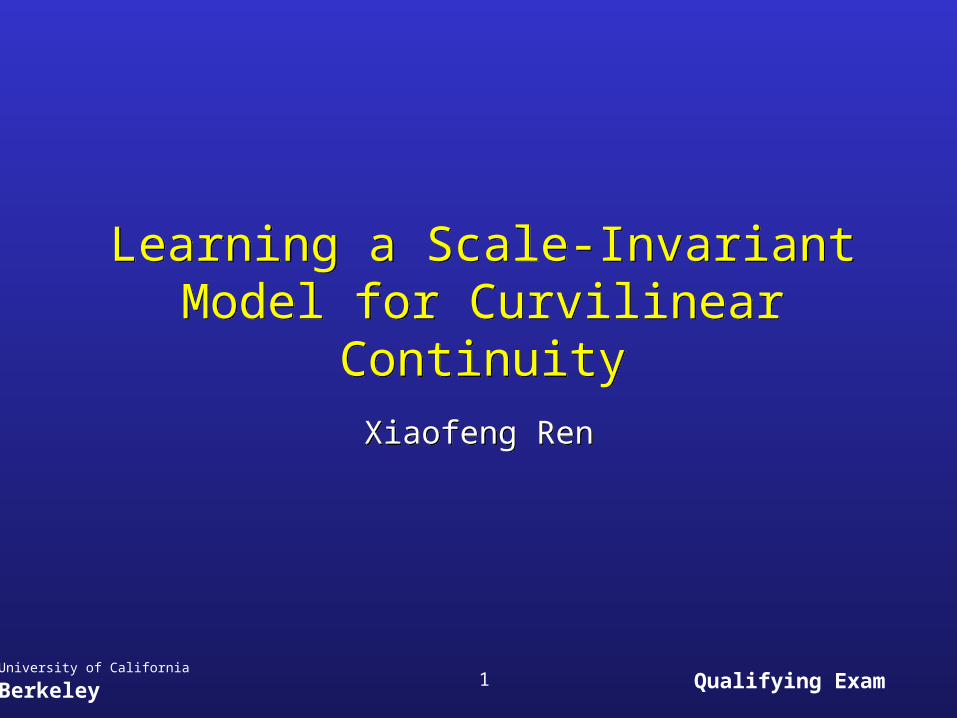
Human-Segmented Natural ImagesHuman-Segmented Natural Images
[Martin et al, ICCV 2001]1,000 images, >14,000 segmentations

10 Qualifying ExamUniversity of California Berkeley
Contour GeometryContour Geometry
• First-Order Markov Model[Mumford 94, Williams & Jacobs 95]
– Curvature: white noise ( independent from position to position )
– Tangent t(s): random walk
– Markov assumption: the tangent at the next position, t(s+1), only depends on the current tangent t(s)
• First-Order Markov Model[Mumford 94, Williams & Jacobs 95]
– Curvature: white noise ( independent from position to position )
– Tangent t(s): random walk
– Markov assumption: the tangent at the next position, t(s+1), only depends on the current tangent t(s)
t(s)
t(s+1)
s
s+1

11 Qualifying ExamUniversity of California Berkeley
Contours are SmoothContours are Smooth
P( t(s+1) | t(s) )
marginal distribution of tangent change
t(s)
t(s+1)
s
s+1

12 Qualifying ExamUniversity of California Berkeley
Testing the Markov AssumptionTesting the Markov Assumption
Segment the contours at high-curvature positions

13 Qualifying ExamUniversity of California Berkeley
If the first-order Markov assumption holds…• At every step, there is a constant probability p that a high curvature
event will occur
• High curvature events are independent from step to step
Let L be the length of a segment between high-curvature points
P( L>=k ) = (1-p)k
P( L=k ) = p(1-p)k
L has an exponential distribution
Prediction: Exponential DistributionPrediction: Exponential Distribution

14 Qualifying ExamUniversity of California Berkeley
Contour segment length L
Pro
babi
lit
y62.1)length(
1.Prob
Empirical Distribution: Power LawEmpirical Distribution: Power Law

15 Qualifying ExamUniversity of California Berkeley
• Power laws widely exist in nature– Brightness of stars– Magnitude of earthquakes– Population of cities– Word frequency in natural languages– Revenue of commercial corporations– Connectivity in Internet topology
… …
• Usually characterized by self-similarity and scale-invariant phenomena
• Power laws widely exist in nature– Brightness of stars– Magnitude of earthquakes– Population of cities– Word frequency in natural languages– Revenue of commercial corporations– Connectivity in Internet topology
… …
• Usually characterized by self-similarity and scale-invariant phenomena
Power Laws in NaturePower Laws in Nature

16 Qualifying ExamUniversity of California Berkeley
• Assume knowledge of contour orientation at coarser scales
• Assume knowledge of contour orientation at coarser scales
t(s)
t(s+1)
2nd Order Markov:
P( t(s+1) | t(s) , t(1)(s+1) )
Higher Order Models:
P( t(s+1) | t(s) , t(1)(s+1), t(2)(s+1), … )
s+1
s
t(1)(s+1)
s+1
Multi-scale Markov ModelsMulti-scale Markov Models
• Coarse-to-fine contour completion• Coarse-to-fine contour completion [Ren & Malik 02]

17 Qualifying ExamUniversity of California Berkeley
Multi-scale Markov:
First-Order Markov:
Contour SynthesisContour Synthesis P( t(s+1) | t(s) )
P( t(s+1) | t(s) , t(1)(s+1), t(2)(s+1), … )
[Ren & Malik 02]
18 Qualifying ExamUniversity of California Berkeley
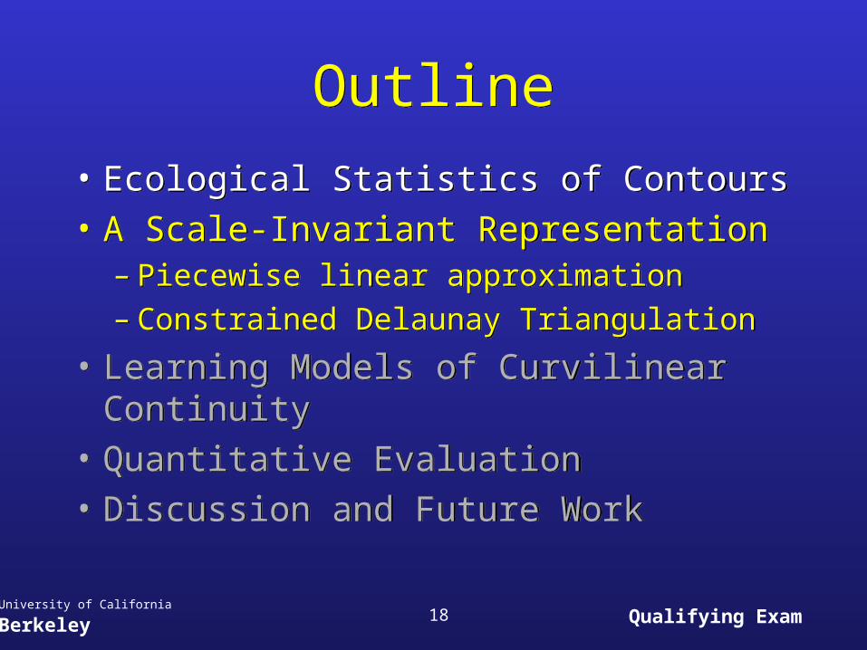
• Ecological Statistics of Contours
• A Scale-Invariant Representation– Piecewise linear approximation– Constrained Delaunay Triangulation
• Learning Models of Curvilinear Continuity
• Quantitative Evaluation
• Discussion and Future Work
• Ecological Statistics of Contours
• A Scale-Invariant Representation– Piecewise linear approximation– Constrained Delaunay Triangulation
• Learning Models of Curvilinear Continuity
• Quantitative Evaluation
• Discussion and Future Work
OutlineOutline

19 Qualifying ExamUniversity of California Berkeley
Local “Probability of Boundary”Local “Probability of Boundary”
• Use Pb (probability of boundary) as input – Combining local brightness, texture and color cues
– Trained from human-marked segmentation boundaries
– Outperform existing local boundary detectors including Canny
• Use Pb (probability of boundary) as input – Combining local brightness, texture and color cues
– Trained from human-marked segmentation boundaries
– Outperform existing local boundary detectors including Canny
[Martin, Fowlkes & Malik 02]

20 Qualifying ExamUniversity of California Berkeley
Piecewise Linear ApproximationPiecewise Linear Approximation• Threshold Pb and find connected boundary pixels
• Recursively split the boundaries until each piece is approximately straight
• Threshold Pb and find connected boundary pixels
• Recursively split the boundaries until each piece is approximately straight
minimize c
a b
c
a
b
Split at C

21 Qualifying ExamUniversity of California Berkeley
Delaunay TriangulationDelaunay Triangulation• Standard in computational geometry
• Dual of the Voronoi Diagram
• Unique triangulation that maximizes the minimum angle– avoiding long skinny triangles
• Efficient and simple randomized algorithm
• Standard in computational geometry
• Dual of the Voronoi Diagram
• Unique triangulation that maximizes the minimum angle– avoiding long skinny triangles
• Efficient and simple randomized algorithm

22 Qualifying ExamUniversity of California Berkeley
Constrained Delaunay TriangulationConstrained Delaunay Triangulation
• A variant of the standard Delaunay Triangulation
• Keeps a given set of edges in the triangulation
• A variant of the standard Delaunay Triangulation
• Keeps a given set of edges in the triangulation
• Still maximizes the minimum angle
• Widely used in geometric modeling and finite elements
• Still maximizes the minimum angle
• Widely used in geometric modeling and finite elements
[Chew 87]
[Shewchuk 96]

23 Qualifying ExamUniversity of California Berkeley
The “Gap-filling” Property of CDTThe “Gap-filling” Property of CDT
• A typical scenario of contour completion• A typical scenario of contour completion
low contrast
high contrasthigh contrast
• CDT picks the “right” edge, completing the gap• CDT picks the “right” edge, completing the gap

24 Qualifying ExamUniversity of California Berkeley
ExamplesExamples
Image Pb CDT

25 Qualifying ExamUniversity of California Berkeley
ExamplesExamples
Black: gradient edges or G-edges
Green: completed edges or C-edges

26 Qualifying ExamUniversity of California Berkeley
• Ecological Statistics of Contours• A Scale-Invariant Representation• Learning Models of Curvilinear Continuity
– Transferring Groundtruth to CDT– A simple model of local continuity– A global model w/ Conditional Random Fields
• Quantitative Evaluation• Discussion and Future Work
• Ecological Statistics of Contours• A Scale-Invariant Representation• Learning Models of Curvilinear Continuity
– Transferring Groundtruth to CDT– A simple model of local continuity– A global model w/ Conditional Random Fields
• Quantitative Evaluation• Discussion and Future Work
OutlineOutline

27 Qualifying ExamUniversity of California Berkeley
Transferring Groundtruth to CDTTransferring Groundtruth to CDT
• Human-marked boundaries are given on the pixel-grid
• Label the CDT edges by bipartite matching
• Human-marked boundaries are given on the pixel-grid
• Label the CDT edges by bipartite matching
Phuman: percentage of pixels
matched to groundtruthhuman-markedboundaries
CDT edges
distance threshold d in matchingd
28 Qualifying ExamUniversity of California Berkeley
Model for ContinuityModel for Continuity
pb0, G0
pb1, G1
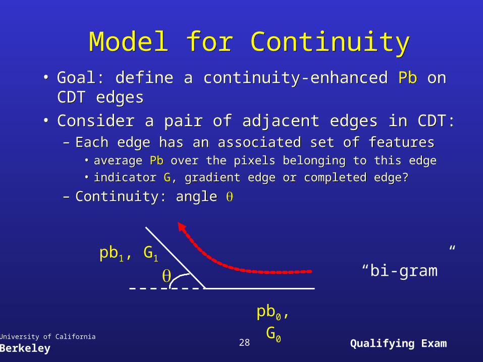
• Goal: define a continuity-enhanced Pb on CDT edges• Consider a pair of adjacent edges in CDT:
– Each edge has an associated set of features• average Pb over the pixels belonging to this edge
• indicator G, gradient edge or completed edge?
– Continuity: angle
• Goal: define a continuity-enhanced Pb on CDT edges• Consider a pair of adjacent edges in CDT:
– Each edge has an associated set of features• average Pb over the pixels belonging to this edge
• indicator G, gradient edge or completed edge?
– Continuity: angle
“bi-gram”
29 Qualifying ExamUniversity of California Berkeley
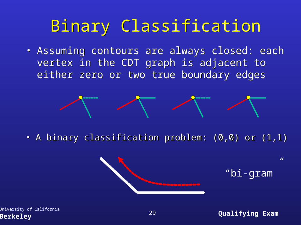
Binary ClassificationBinary Classification• Assuming contours are always closed: each vertex in the CDT
graph is adjacent to either zero or two true boundary edges• Assuming contours are always closed: each vertex in the CDT
graph is adjacent to either zero or two true boundary edges
• A binary classification problem: (0,0) or (1,1) • A binary classification problem: (0,0) or (1,1)
“bi-gram”

30 Qualifying ExamUniversity of California Berkeley
Learning Local ContinuityLearning Local Continuity
• Binary classification: (0,0) or (1,1)• Transferred Groundtruth labels on CDT edges
• Features:– average Pb
– (G0*G1): both are gradient edges?
– angle
• Logistic regression
• Binary classification: (0,0) or (1,1)• Transferred Groundtruth labels on CDT edges
• Features:– average Pb
– (G0*G1): both are gradient edges?
– angle
• Logistic regression
pb0, G0
pb1, G1

31 Qualifying ExamUniversity of California Berkeley
PbL: Pb + Local ContinuityPbL: Pb + Local Continuity
pb0, G0
pb1, G1
1
pb2, G2
2
L LPbL
=
Evidence of continuity comes from both ends
take max. over all possible pairs

32 Qualifying ExamUniversity of California Berkeley
Variants of the Local ModelVariants of the Local Model
• More variants of the local model
– alternative classifiers ( SVM, HME, … )
– 4-way classification
– additional features
– learning a 3-edge (tri-gram) model
– learning how to combine evidence from both ends
• No significant improvement in performance
• More variants of the local model
– alternative classifiers ( SVM, HME, … )
– 4-way classification
– additional features
– learning a 3-edge (tri-gram) model
– learning how to combine evidence from both ends
• No significant improvement in performance
33 Qualifying ExamUniversity of California Berkeley
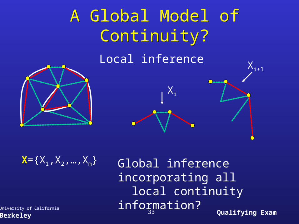
A Global Model of Continuity?A Global Model of Continuity?
Global inference incorporating all local continuity information?
X={X1,X2,…,Xm}
Local inference
Xi
Xi+1

34 Qualifying ExamUniversity of California Berkeley
Conditional Random FieldsConditional Random Fields
For each edge i, define a set of features{g1,g2,…,gh}
Potential function exp(i) at edge i
hhi ggg 2211expexp
For each junction j, define a set of features{f1,f2,…,fk}
Potential function exp(j) at juncion j
kkj fff 2211expexp
X={X1,X2,…,Xm}
[Pietra, Pietra & Lafferty 97][Lafferty, McCallum & Pereira 01]

35 Qualifying ExamUniversity of California Berkeley
Conditional Random FieldsConditional Random Fields
X={X1,X2,…,Xm}
Potential function on edges {exp(i)}
Potential function on junctions {exp(j)}
This defines a probability distribution over X:
X j
ji
i XXZ exp
Z
XX
XPj
ji
i exp
whereEstimate P(Xi|)

36 Qualifying ExamUniversity of California Berkeley
Buliding a CRF ModelBuliding a CRF Model
• What are the features?– edge features are easy: Pb, G
– junction features: type and continuity
• How to make inference?
• How to learn the parameters?
• What are the features?– edge features are easy: Pb, G
– junction features: type and continuity
• How to make inference?
• How to learn the parameters?X={X1,X2,…,Xm}
Estimate P(Xi|)

37 Qualifying ExamUniversity of California Berkeley
Junction Features in CRFJunction Features in CRF• Junction types (degg,degc):• Junction types (degg,degc):
baXf cgba degdeg),(
degg=1,degc=0 degg=0,degc=2 degg=1,degc=2
• Continuity term for degree-2 junctions• Continuity term for degree-2 junctions
degg=0,degc=2
),(),( exp baba f
2degdeg exp cgg degg=0,degc=2

38 Qualifying ExamUniversity of California Berkeley
Inference w/ Belief PropagationInference w/ Belief Propagation
• Belief Propagation– Xi: state of the node (edge) i
– Fq: state of the factor (junction) q
– potentials on Xi,Xj,Xk, Fq={Xi, Xj, Xk}
– want to compute PbG=P(Xi)
– mqi: “belief” about Xi from Fq
• Belief Propagation– Xi: state of the node (edge) i
– Fq: state of the factor (junction) q
– potentials on Xi,Xj,Xk, Fq={Xi, Xj, Xk}
– want to compute PbG=P(Xi)
– mqi: “belief” about Xi from Fq
• The CDT graph has many loops in it• The CDT graph has many loops in it
Fq
Xj
Xk
Xi
mkq
mjq
mqi
kji XXXkkqjjqkjii
qiqi XmXmXXX
ZXm
,,
,,1
Fr
mir
iX
iqiiii
iir XmXZ
Xm 1

39 Qualifying ExamUniversity of California Berkeley
Inference w/ Loopy Belief PropagationInference w/ Loopy Belief Propagation
• Loopy Belief Propagation
– just like belief propagation
– iterates message passing until convergence
– lack of theoretical foundations and known to have convergence issues
– however becoming popular in practice
– typically applied on pixel-grid
• Works well on CDT graphs– converges fast
– produces empirically sound results
• Loopy Belief Propagation
– just like belief propagation
– iterates message passing until convergence
– lack of theoretical foundations and known to have convergence issues
– however becoming popular in practice
– typically applied on pixel-grid
• Works well on CDT graphs– converges fast
– produces empirically sound results[Berrou 93], [Freeman 98], [Murphy 99], [Weiss 97,99,01]
40 Qualifying ExamUniversity of California Berkeley
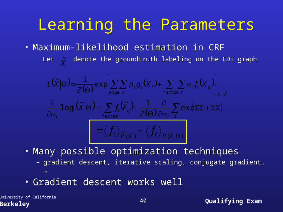
Learning the ParametersLearning the Parameters
• Maximum-likelihood estimation in CRFLet denote the groundtruth labeling on the CDT graph
• Maximum-likelihood estimation in CRFLet denote the groundtruth labeling on the CDT graph
XXq
qtt
ti
iss
s XfXgZ
XL~factor edge
exp1~
Xtqqt
t ZFfXL exp
1~~log
factor
• Many possible optimization techniques– gradient descent, iterative scaling, conjugate gradient, …
• Gradient descent works well
• Many possible optimization techniques– gradient descent, iterative scaling, conjugate gradient, …
• Gradient descent works well
X~
)|()(~
XPtXPt ff

41 Qualifying ExamUniversity of California Berkeley
Interpreting the ParametersInterpreting the Parameters
• The junction parameters (degg,degc) on the horse dataset:• The junction parameters (degg,degc) on the horse dataset:
(0,0)= 2.8318
(1,0)= 1.1279
(2,0)= 1.3774
(3,0)= 0.0342
(2,0)= 1.3774
(1,1)= -0.6106
(0,2)= -0.9773
there are more non-boundary edges than boundary edges
a continuation is better than a line-ending
junctions are rare
G-edges are better for continuation than C-edges

42 Qualifying ExamUniversity of California Berkeley
• Ecological Statistics of Contours
• A Scale-Invariant Representation
• Learning Models of Curvilinear Continuity
• Quantitative Evaluation– The precision-recall framework– Experimental results on three datasets
• Discussion and Future Work
• Ecological Statistics of Contours
• A Scale-Invariant Representation
• Learning Models of Curvilinear Continuity
• Quantitative Evaluation– The precision-recall framework– Experimental results on three datasets
• Discussion and Future Work
OutlineOutline

43 Qualifying ExamUniversity of California Berkeley
DatasetsDatasets
• Baseball player dataset [Mori et al 04]
– 30 news photos of baseball players in various poses, 15 training and 15 testing
• Horse dataset [Borenstein & Ullman 02]
– 350 images of standing horses facing left, 175 training and 175 testing
• Berkeley Segmentation Dataset [Martin et al 01]
– 300 Corel images of various natural scenes and ~2500 segmentations, 200 training and 100 testing

44 Qualifying ExamUniversity of California Berkeley
Evaluating Boundary OperatorsEvaluating Boundary Operators• Precision-Recall Curves [Martin, Fowlkes & Malik 02]
– threshold the output boundary map
– bipartite matching with the groundtruth
• Precision-Recall Curves [Martin, Fowlkes & Malik 02]– threshold the output boundary map
– bipartite matching with the groundtruth
m pixels on human-marked boundaries
n detected pixels above a given threshold
k matched pairs
Precision = k/n, percentage of true positives
Recall = k/m, percentage of groundtruth being detected
• Project CDT edges back to the pixel-grid• Project CDT edges back to the pixel-grid

45 Qualifying ExamUniversity of California Berkeley
No Loss of Structure in CDTNo Loss of Structure in CDT
Use Phuman the soft groundtruthlabel defined on CDT graphs:precision close to 100%
Pb averaged over CDT edges: no worse than the orignal Pb

46 Qualifying ExamUniversity of California Berkeley
Continuity improves boundary detection in both low-recall and high-recall ranges
Global inference helps; mostly in low-recall/high-precision
Roughly speaking,
CRF>Local>CDT only>Pb

47 Qualifying ExamUniversity of California Berkeley

48 Qualifying ExamUniversity of California Berkeley

49 Qualifying ExamUniversity of California Berkeley
Image Pb Local Global

50 Qualifying ExamUniversity of California Berkeley
Image Pb Local Global
51 Qualifying ExamUniversity of California Berkeley
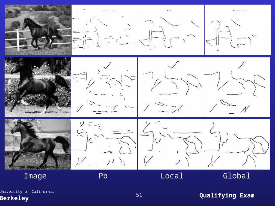
Image Pb Local Global
52 Qualifying ExamUniversity of California Berkeley
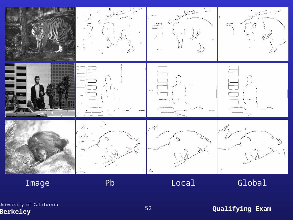
Image Pb Local Global

53 Qualifying ExamUniversity of California Berkeley
In Conclusion…In Conclusion…• Boundary contours are scale-invariant in nature;• Boundary contours are scale-invariant in nature;• Constrained Delaunay Triangulation is a scale-invariant
discretization of images with little loss of structure;• Constrained Delaunay Triangulation is a scale-invariant
discretization of images with little loss of structure;
• Moving from 100,000 pixels to <1000 edges, CDT achieves great statistical and computational efficiency;
• Moving from 100,000 pixels to <1000 edges, CDT achieves great statistical and computational efficiency;
• Curvilinear Continuity improves boundary detection;
– the local model of continuity is simple yet very effective
– global inference of continuity further improves performance
– Conditional Random Fields w/ loopy belief propagation works well on CDT graphs
• Curvilinear Continuity improves boundary detection;
– the local model of continuity is simple yet very effective
– global inference of continuity further improves performance
– Conditional Random Fields w/ loopy belief propagation works well on CDT graphs
• Mid-level vision is useful.• Mid-level vision is useful.

54 Qualifying ExamUniversity of California Berkeley
Future WorkFuture Work• To add more features into CRF
– region-based features
– avoiding spurious completions
– tri-gram model
• To train CRF w/ different criteria– e.g., area under the precision-recall curve
– Max-margin Markov networks
• To use CRF for feature selection
• To apply CDT+CRF to other mid-level vision problems, e.g., figure/ground organization
• To add more features into CRF– region-based features
– avoiding spurious completions
– tri-gram model
• To train CRF w/ different criteria– e.g., area under the precision-recall curve
– Max-margin Markov networks
• To use CRF for feature selection
• To apply CDT+CRF to other mid-level vision problems, e.g., figure/ground organization

55 Qualifying ExamUniversity of California Berkeley
Figure/Ground OrganizationFigure/Ground Organization
• A classical problem in Gestalt psychology[Rubin 1921]
• “Perceptual organization after grouping”
• Gestalt principles for figure/ground– surroundedness, size, convexity, parallelism, symmetry,
lower-region, common fate, familiar configuration, …
• Very few computational studies[Hinton 86], [von der Heydt 93]

56 Qualifying ExamUniversity of California Berkeley
Using Shapemes for Figure/GroundUsing Shapemes for Figure/Ground
• To capture mid-level information:
“local” shape configuration
• To capture mid-level information:
“local” shape configuration
• Shape context [Belongie, Malik & Punicha 01]
• Clustering shape context into prototypical shape configurations or “shapemes”
• Local figure/ground discrimination with shapemes
• Shape context [Belongie, Malik & Punicha 01]
• Clustering shape context into prototypical shape configurations or “shapemes”
• Local figure/ground discrimination with shapemes

57 Qualifying ExamUniversity of California Berkeley
ShapemesShapemes

58 Qualifying ExamUniversity of California Berkeley
Junction Types for Figure/GroundJunction Types for Figure/Ground
F
G
F
F
GG
common
F
G
F
G
GF
uncommon

59 Qualifying ExamUniversity of California Berkeley
CRF for Figure/GroundCRF for Figure/Ground
F={F1,F2,…,Fm}
Fi{Left,Right} • Add a continuity term
F
G
F
F
GG
• One feature for each junction type

60 Qualifying ExamUniversity of California Berkeley
Preliminary Results on Figure/GroundPreliminary Results on Figure/Ground
• Chance error rate• Local operator w/ shapemes
• Using human segmentations:– Averaging local cues on human-
marked boundaries
– CRF w/ junction type
– CRF w/ junction type and continuity
• To use CDT graphs
• Chance error rate• Local operator w/ shapemes
• Using human segmentations:– Averaging local cues on human-
marked boundaries
– CRF w/ junction type
– CRF w/ junction type and continuity
• To use CDT graphs
50%
39%
29%
28%
21%
50%
39%
29%
28%
21%

61 Qualifying ExamUniversity of California Berkeley
Thank You

62 Qualifying ExamUniversity of California Berkeley