Embed Size (px)
Citation preview

Learning a decision maker’s utility function
from (possibly) inconsistent behavior
Thomas D. Nielsen and Finn V. Jensen
Department of Computer Science, Aalborg University, Fredrik Bajers Vej 7E,
DK-9220 Aalborg Ø, Denmark
Abstract
When modeling a decision problem using the influence diagram framework, thequantitative part rests on two principal components: probabilities for representingthe decision maker’s uncertainty about the domain and utilities for representingpreferences. Over the last decade, several methods have been developed for learningthe probabilities from a database. However, methods for learning the utilities haveonly received limited attention in the computer science community.
A promising approach for learning a decision maker’s utility function is to takeoutset in the decision maker’s observed behavioral patterns, and then find a utilityfunction which (together with a domain model) can explain this behavior. Thatis, it is assumed that decision maker’s preferences are reflected in the behavior.Standard learning algorithms also assume that the decision maker is behavioralconsistent, i.e., given a model of the decision problem, there exists a utility functionwhich can account for all the observed behavior. Unfortunately, this assumption israrely valid in real-world decision problems, and in these situations existing learn-ing methods may only identify a trivial utility function. In this paper we relax thisconsistency assumption, and propose two algorithms for learning a decision maker’sutility function from possibly inconsistent behavior; inconsistent behavior is inter-preted as random deviations from an underlying (true) utility function. The maindifference between the two algorithms is that the first facilitates a form of batchlearning whereas the second focuses on adaptation and is particularly well-suited forscenarios where the DM’s preferences change over time. Empirical results demon-strate the tractability of the algorithms, and they also show that the algorithmsconverge toward the true utility function for even very small sets of observations.
Key words: Influence diagram, learning utility functions, inconsistent behavior.
Email addresses: [email protected] (Thomas D. Nielsen), [email protected] (FinnV. Jensen).
Preprint submitted to Elsevier Science 16 August 2004

1 Introduction
When modeling a decision problem using the influence diagram framework(Howard and Matheson, 1981) we need to specify both a qualitative part(represented by a acyclic directed graph) and a quantitative part. The quanti-tative part is comprised of probabilities which represent the decision maker’s(DM’s) uncertainty about the domain, and utilities which represent the DM’spreferences about the different outcomes of the decision problem.
The specification of the quantitative part of the model constitutes one ofthe main difficulties when modeling a decision problem using the influencediagram representation. Over the last decade, research has focused on learningthe probabilities from a database (see e.g. Buntine (1996) for an overview),however, automatic learning of the utilities has received less attention. Forsequential decision problems, this task was first addressed by Sargent (1978)within the economics community. Sargent (1978) considered the problem ofestimating (among other parameters) the cost of adjusting the daytime andovertime labor force by observing a firm’s labor demand. In a more generalcontext, there has been an increasing interest in techniques for structuralestimation of Markov decision processes (MDPs), see (Rust, 1994) and thereferences within. For instance, Keane and Wolpin (1997) estimates a dynamicmodel for schooling, work and occupational choice of young men.
In general, current approaches for semi-automatic learning of a DM’s utilityfunction have focused on three different areas: i) eliciting the utility functionof the DM based on a database of already elicited utility functions (Chajewskaet al., 1998; Chajewska and Koller, 2000), ii) iterative refinement of the DM’scurrent utility function using a value of information approach (Chajewskaet al., 2000), and iii) eliciting the utility function based on a database ofobserved behavioral patterns (Rust, 1994; Suryadi and Gmytrasiewicz, 1999;Ng and Russell, 2000; Chajewska et al., 2001). The latter approach is basedon the assumption that the DM’s “true” utility function is reflected in theobserved behavior.
In this paper we focus on the third category within the framework of influencediagrams, i.e., learning a DM’s utility function from her observed behavioralpatterns. Unfortunately, the estimation techniques for MDPs cannot directlybe applied to frameworks such as influence diagrams, although some of theideas carry over. Moreover, existing ID learning methods are based on the as-sumptions that the model provides an accurate representation of the problemdomain, and that the DM is an expected utility maximizer always with thesame von Neuman-Morgenstern utility function.1 These assumptions, how-
1 Together, these two assumptions imply that the DM is behavioral consistent, i.e.,given a model of the decision problem, there exists a utility function which can
2

ever, are rarely valid in practice. For example, humans rarely behave as tomaximize the expected utility w.r.t. a certain model (Allais, 1979), and theutility function of a DM may fluctuate and/or change permanently over time.As a consequence, traditional learning methods may only be able to identify atrivial utility function (i.e., a utility function giving the same utility to all out-comes), but this type of utility function is hardly an appropriate descriptionof the DM’s preferences.
In this paper we relax the assumptions above, and propose two algorithms forlearning the “true” utility function of a DM by observing possibly inconsis-tent behavior, i.e., behavior which cannot be explained by a non-trivial utilityfunction.2 The first algorithm can be characterized as a batch learning pro-cedure whereas the second algorithm focuses on adaptation. The assumptionunderlying both of the proposed algorithms is that inconsistent behavior canbe explained as random deviations from an underlying true utility functionwhich is the one we would like to estimate.
A promising feature of the proposed algorithms follows from the fact thata given observation-decision sequence truncates the space of possible utilityfunctions. Hence, we would in general expect that even a small database canbe used to learn a reasonable approximation of the DM’s true utility function.That this is also the case is confirmed by several empirical experiments, whereit is also shown that the algorithms are even robust to deviations from theunderlying utility model. This observation also points to another possible ap-plication area, namely adaptive agents in e.g. computer games. That is, agentswhich can adapt to the behavior of other computer controlled agents as wellas avatars. In these types of domains we usually have very limited amounts ofdata for the individual agents, thereby making it difficult to apply traditionalmachine learning algorithms when performing learning or adaptation.
The remainder of this paper is organized as follows. In Section 2 we describethe framework of influence diagrams and introduce some of the terms andnotation used throughout the paper. In Section 3 we pose the general prob-lem of learning a DM’s utility function and we outline some existing learningalgorithms. Section 4 discusses a utility model for explaining inconsistent be-havior, and based on this model we propose two algorithms for learning autility function from possibly inconsistent behavior; the first algorithm is abatch learning procedure whereas the second algorithm provides a methodfor doing adaptation. In Section 5 we present several empirical results whichdemonstrate the applicability of both algorithms. Finally, in Section 6 we dis-cuss some optimization issues and point to areas for future research.
account for all the observed behavior.2 See Rust (1994) for a discussion of this problem in the context of MDPs, whereinconsistent behavior is attributed to unobserved state variables.
3

2 Influence diagrams
An influence diagram (ID) can be seen as a Bayesian network (BN) augmentedwith decision nodes and value nodes, where value nodes have no descendants.Thus, an ID is a acyclic directed graph G = (U , E), where the nodes U canbe partitioned into three disjoint subsets; chance nodes UC, decision nodes UDand value nodes UV.
In the remainder of this paper we assume a total ordering of the decisionnodes, indicating the order in which the decisions are made (the orderingof the decision nodes is traditionally represented by a directed path whichincludes all decision nodes). Furthermore, we will use the concept of node andvariable interchangeably if this does not introduce any inconsistency. We willalso assume that no barren nodes are specified by the ID since they have noimpact on the decisions, see Shachter (1986); a chance node or a decision nodeis said to be barren if it has no children, or if all its descendants are barren.
With each chance variable and decision variable X we associate a state space
sp (X) which denotes the set of possible outcomes/decision options for X. Fora set U ′ of chance variables and decision variables we define the state space assp (U ′) = ×{sp (X) |X ∈ U ′}, where A×B denotes the Cartesian product of Aand B. The uncertainty associated with each chance variable C is representedby a conditional probability potential P(C|pa (C)) : sp ({C} ∪ pa (C)) → [0; 1],where pa (C) denotes the parents of C in the ID. The domain of a conditionalprobability potential φC = P(C|pa (C)) is denoted dom (φC) = {C} ∪ pa (C).
The DM’s preferences are described by a multi-attribute utility potential, andin the remainder of this paper we shall assume that this utility potential islinearly-additive with equal weights, see e.g. Tatman and Shachter (1990).The set of value nodes UV defines the set of utility potentials which appearas additive components in the multi-attribute utility potential.3 Each utilitypotential indicates the local utility for a given configuration of the variablesin its domain. The domain of a utility potential ψV is denoted dom (ψV) =
pa (V), where V is the value node associated with ψV. Analogously to theconcepts of variable and node we shall sometimes use the terms value nodeand utility potential interchangeably.
A realization of an ID, I, is an attachment of potentials to the appropriatevariables in I, i.e., a realization is a set {P(C|pa (C))|C ∈ UC}∪{ψV(pa (V))|V ∈UV}. So, a realization specifies the quantitative part of the model whereas theID constitutes the qualitative part.
3 Note that Tatman and Shachter (1990) also consider the case where the utility isdefined as the product of a set of utility potentials; such a utility potential can betransformed to decompose additively by taking the logarithm of the utilities.
4

The arcs in an ID can be partitioned into three disjoint subsets, correspondingto the type of node they go into. Arcs into value nodes represent functionaldependencies by indicating the domain of the associated utility potential. Arcsinto chance nodes, termed dependency arcs, represent probabilistic dependen-cies, whereas arcs into decision nodes, termed informational arcs, imply in-formation precedence; if there is an arc from a node X to a decision node D,then the state of X is known when decision D is made.
Let UC be the set of chance variables and let UD = {D1, D2, . . . , Dn} be theset of decision variables. Assuming that the decision variables are orderedby index, the set of informational arcs induces a partitioning of UC into acollection of disjoint subsets C0, C1, . . . , Cn. The set Cj denotes the chancevariables observed between decision Dj and Dj+1. Thus the variables in Cjoccur as immediate predecessors of Dj+1. This induces a partial order ≺ onUC ∪ UD, i.e., C0 ≺ D1 ≺ C1 ≺ · · · ≺ Dn ≺ Cn.The set of variables known to the decision maker when deciding on Dj is calledthe informational predecessors of Dj and is denoted pred (Dj). By assumingthat the decision maker remembers all previous observations and decisions,we have pred (Di) ⊆ pred (Dj) (for Di ≺ Dj) and in particular, pred (Dj)is the variables that occur before Dj under ≺. This property is known asno-forgetting and from this we can assume that an ID does not contain anyno-forgetting arcs, i.e., pa (Di) ∩ pa (Dj) = ∅ if Di 6= Dj.2.1 Evaluation
When evaluating an ID we identify a strategy for the decisions involved; astrategy can be seen as a prescription of responses to earlier observationsand decisions. The evaluation is usually performed according to the maxi-
mum expected utility principle, which states that we should always choose analternative that maximizes the expected utility.
Definition 1. Let I be an ID and let UD denote the decision variables in I.A strategy is a set of functions ∆ = {δD|D ∈ UD}, where δD is a policy givenby:
δD : sp (pred (D)) → sp (D) .
A strategy that maximizes the expected utility is termed an optimal strategy,and each policy in an optimal strategy is termed an optimal policy.
5

The optimal policy for the last decision variable Dn is given by:4
δDn(C0, D1, . . . , Dn-1,Cn-1)= arg maxDn ∑
Cn P(Cn|C0, D1, . . . , Cn-1, Dn) ∑V∈UVψV.Similarly, the maximum expected utility for decision Dn is
ρDn(C0, D1, . . . , Dn-1, Cn-1) = maxDn ∑
Cn P(Cn|C0, D1, . . . , Cn-1, Dn) ∑V∈UVψV.(1)
In general, the optimal policy for a decision variable Dk is given by:
δDk(C0, D1, . . . , Dk-1, Ck-1) = arg maxDk ∑
Ck P(Ck|C0, D1, . . . , Ck-1, Dk)ρDk+1,(2)
where ρDk+1 is the maximum expected utility potential for decision Dk+1:ρDk+1(C0, D1, . . . , Dk, Ck) = maxDk+1 ∑
Ck+1 P(Ck+1|C0, D1, . . . , Ck, Dk+1)ρDk+2.If we suppress the maximization over Dk+1, we obtain the expected utility
potential for decision Dk+1:ρ(Dk+1, C0, D1, . . . , Dk, Ck) =
∑
Ck+1 P(Ck+1|C0, D1, . . . , Ck, Dk+1)ρDk+2. (3)
The optimal policy for a decision variable, Dk, is in principle a function overthe entire past of Dk (i.e. pred (Dk)). However, not all the variables observeddo necessarily influence the optimal policy for Dk, hence we introduce thenotion of a required variable:
Definition 2. Let I be an ID and let D be a decision variable in I. Thevariable X ∈ pred (D) is said to be required for D if there exists a realizationof I, a configuration y over dom (δD) \{X}, and two states x1 and x2 of X s.t.δD(x1, y) 6= δD(x2, y). The set of variables required for D is denoted req (D).
Different algorithms for identifying the required variables have been proposedby Shachter (1999), Nielsen and Jensen (1999) and Lauritzen and Nilsson(2001). For example, the algorithm by Shachter (1999) traverse the decisionvariables in reverse temporal order. When a decision variable is visited itsrequired past is determined and the decision variable is then substituted by achance variable having the required variables as parents:
4 For the sake of simplifying notation we shall assume that for all decision variablesDi there is always exactly one element in arg maxDi (·).
6

Definition 3. Let D be a decision variable and let δD(req (D)) be an optimalpolicy for D. A chance variable D ′ with req (D) as parents and with theprobability potential P(D ′|req (D)) defined as:
P(d|π) =
{1 if δD(π) = d,
0 otherwise
is said to be the chance variable representation of δD.
Thus, we only need to (iteratively) determine the required variables for thelast decision variable Dn. For this decision variable it can be shown that avariable X ∈ pred (Dn) is required for Dn if and only if X is d-connected to autility descendant of Dn given pred (Dn) \ {X}.
3 Observed behavior as utility constraints
Consider an influence diagram, I, modeling some decision problem, wherethe DM’s preferences are expressed by a utility function ψ. Given this influ-ence diagram representation, the DM’s observed behavior can be seen as anobservation-decision sequence (or behavioral pattern) w.r.t. the variables in I;for each decision D we have a configuration over the set of variables which iscomprised of D and the variables which are observed immediately before D.Such an observation-decision sequence is necessarily consistent with at leastone strategy ∆ ′, and we therefore introduce the notion of an instantiation ofa strategy.
Definition 4. Let I be an ID and let ∆ be a strategy for the decision variablesin I. Let I ′ be the BN obtained from I (value nodes are ignored) by replacing alldecision variables in I with chance variable representations of their policies in ∆(see Definition 3). A configuration c over the variables ∪D∈UD(req (D)∪{D}) isthen said to be an instantiation of ∆ if P ′(c) > 0, where P ′(·) is the probabilitydistribution encoded by I ′.
Definition 5. Let I be an ID and let ψ be a utility function for I. If ∆ is anoptimal strategy for I w.r.t. ψ and c is an instantiation of ∆, then c is said tobe an instantiation of I w.r.t. ψ (or ψ induces c). For a set D = {c1, . . . , cN}
of instantiations we say that ψ induces D if ψ induces ci, for all 1 ≤ i ≤ N.
Obviously, for any utility function we may have several different instantiationsw.r.t. the utility function in question. Moreover, for any instantiation c we donot have a unique utility function inducing c, since a utility function is onlyunique up to a positive affine transformation. Note that if the optimal strategyis not required to be strictly optimal, then any instantiation may be induced
7

by a trivial utility function (a utility function giving the same utility to alloutcomes).
Assume now that we have a database D = {c1, . . . , cN} of observed behavioralpatterns for some DM; this corresponds to the situation where the DM isrepeatedly confronted with the same decision problem e.g. a doctor diagnosingand treating patients. Given that the DM is an expected utility maximizer,always with the same von Neuman-Morgenstern utility function, an obviousapproach for identifying a representation of the utility function which inducesD would be to investigate the set ΨD of candidate utility functions:
ΨD = {ψ|ψ induces ci, ∀1 ≤ i ≤ N}. (4)
If the database encodes an entire strategy, then we can easily find this setof candidate utility functions: Start off by substituting each decision variablewith its chance variable representation as encoded by the cases in D (seeDefinition 3). Next, consider the last decision variable Dn and assume thatcase c specifies {Dn} ∪ req (Dn) = (d, πDn) that is, c
#fDng∪req(Dn) = (d, πDn).This gives us:
ρ(d, πDn) ≥ ρ(d ′, πDn), ∀d ′ ∈ sp (Dn) \ {d}. (5)
From Equation 1, the expected utility function for the last decision is givenby:
ρ(Dn, req (Dn)) =∑
Cn P(Cn|Dn, pred (Dn)) ∑V∈UVψV(pa (V))
=∑
Cn P(Cn|Dn, req (Dn)) ∑V∈UVψV(pa (V))
=∑V∈UV ∑
Cn P(Cn|Dn, req (Dn))ψV(pa (V))
=∑V∈UV ∑
Cn∩pa(V)ψV(pa (V))∑
Cnnpa(V)P(Cn|Dn, req (Dn))=
∑V∈UV ∑
Cn∩pa(V)ψV(pa (V))P(Cn ∩ pa (V) |Dn, req (Dn)).(6)
Thus, for any configuration (d, πDn) over {Dn} ∪ req (Dn) the expected util-ity is linear in the utilities, and Inequality 5 therefore defines a set of linearconstraints for the utility function. Moreover all the coefficients for the inequal-ities can be found by instantiating the corresponding variables and performingone outward propagation in the strong junction tree representation of the ID(Jensen et al., 1994; Madsen and Jensen, 1999); from the construction of thestrong junction tree we are guaranteed that at least one clique contains pa (V)
8

from which P(Cn∩pa (V) |d, πDn) can directly be read. Finally, as all decisionvariables have been substituted with their chance variable representations wecan perform the analysis above for each decision variable by moving in re-verse temporal order. This also implies that in order to find a set of candidateutility functions we simply need to solve the collection of linear inequalitiesidentified during the analysis. Unfortunately this approach relies on the entirestrategy to be encoded in the database which is very unlikely to happen inpractice. When only a partial strategy is described by the database, then theconstraints specified by the observed behavior are no longer linear and theabove procedure cannot be applied. This can easily be seen by noticing thatfor any unobserved configuration of the required past for a decision variable,we need to apply a maximization when eliminating that variable; the expectedutility function for a decision variable in the required past for that variable willtherefore no longer be linear (we shall return to this discussion in Section 6).
Now assume that we are given a set of candidate utility functions, and wewould like to reason about the DM preferences. One approach would be toselect one of the candidate utility functions as a representation of the DM’sunknown utility function; by the assumptions above we are guaranteed thatsuch a utility function exists. This approach has been pursued by e.g. Suryadiand Gmytrasiewicz (1999) who propose an adaptation scheme where a singleutility function is found by using a method similar to the delta rule for learningneural networks. Ng and Russell (2000) propose heuristics for discriminatingamong the different candidate utility functions in the context of Markov de-cision processes. Alternatively, Chajewska et al. (2001) derive a procedure forestimating a probability distribution over the candidate utility functions. Theapproach by Chajewska et al. (2001) is based on specifying a prior proba-bility distribution for the utilities, and then applying a Markov Chain MonteCarlo technique for sampling from this truncated distribution; the distributionis truncated according to the constraints imposed by the observed behavior.Note that both Ng and Russell (2000) and Chajewska et al. (2001) considerthe situation when the optimal strategy is fully observed as well as when it isonly partially observed.
Unfortunately, the assumptions underlying the methods referenced above arerarely valid in real world decision problems: (i) the ID model may not pro-vide an accurate description of the decision problem, see e.g. (Rust, 1994;Shachter and Mandelbaum, 1996), (ii) the DM’s preferences may fluctuateand/or change permanently over time, and (iii) human DMs do not alwaysbehave as to maximize the expected utility (Allais, 1979; Kahneman and Tver-sky, 1979). In these situations, the observed behavior of the DM may appearinconsistent w.r.t. the ID in question, i.e., there may not exist a non-trivialutility function for the ID which satisfies all the constraints implied by theobserved behavior. As a consequence, existing learning methods would onlyidentify a trivial utility function which is inadequate for e.g. reasoning about
9

the future behavior of the DM. Note that this problem has previously beenconsidered in the context of MDPs (Rust, 1994), where discrepancies in theobservation-decision sequences are attributed to the occurrence of unobservedstate variables. In this setting, the parameters are estimated by maximizing(using a nested fixed point algorithm) the likelihood function for the observedbehavior.
In what follows we establish a utility model which accommodates situation(i) and (ii); as a special case, the model also includes the situation where theprevious stated assumptions do hold. Based on this model we propose twomethods for learning a DM’s utility function by observing (possibly) inconsis-tent behavioral patterns. The discussion of (iii) is postponed until Section 6,where the model is briefly discussed in relation to the rank dependent utility
model by Quiggin (1982).
4 Learning a utility function from inconsistent behavior
In the proposed utility model, it is assumed that the DM has an underlying(true) utility function (denoted ψ∗) and that any type of inconsistent behaviorcan be explained as deviations from ψ∗.5 More precisely, consider a databaseof cases D = {c1, . . . , cN} from an ID I. In the proposed model, each case ci isassumed to be an instantiation of I w.r.t. some utility function ψci obtainedfrom ψ∗ by adding some white noise. Hence, each case, ci, is an instantiationof an optimal strategy found w.r.t. the utility function ψci generated fromψ∗; for each outcome o, we have ψci(o) = ψ∗(o)+ǫo, where ǫo has a normaldistribution with zero mean and variance σ2o. Hence, by assuming that thenoise associated with the utilities are marginally independent, and that thevariance only depends on the outcome in question we get
ψci =∑V∈UVψciV =
∑V∈UV(ψ∗V + ǫciV ), (7)
where ǫciV (o#pa(V)) ∼ N(0, σ2o#pa(V)). Note that we implicit assume that ψcidecomposes additively in the same factors as ψ∗. A graphical representationof the utility model (with m utility parameters in the true utility function) isillustrated in Fig. 1, where the nodes c1, . . . , cN are information nodes thatencode the observed behavior; the independence statements can be deducedin the usual fashion.
5 This assumption can also be seen in relation to (i) as well as the discussion byShachter and Mandelbaum (1996) who argue that uncertainties in the model canbe encoded in the utility function.
10

ψ∗1 σ21 ψ∗m σ2mψc11 ψc21 ψcN1 ψc1m ψc2m ψcNm
c1 c2 cNFig. 1. A graphical representation of the utility model for encoding inconsistentbehavior.
Thus, for each parameter, ψ∗j , in the true utility function we have a variance,
σ2j , and a corresponding utility parameter, ψcij , for each case ci. Note thatthe model does not make any assumptions about the type of prior probabilitydistribution of the true utility function and the variance of the parameters.Moreover, the model facilitates an easy way to encode prior information aboutthe DM’s preferences. For instance, given that we have the prior informationthat oi ≺ oj, then we can take this information into account by simply spec-ifying ψ∗(oi) < ψ∗(oj); thus changing the independence statements in themodel, making it a chain graph.
Each constraint induced by an observed behavioral pattern specifies the setof candidate utility functions for the corresponding case. Given a prior prob-ability distribution for the true utility function, we can then, in principle, usethe set, D, of cases to obtain a posterior probability distribution P(ψ∗|D) forthe true utility function. In turn, this probability distribution can be used tocalculate the expected value of each parameter in the true utility function,which could be used as a representation of the DM’s actual utility function.
Unfortunately, even if the prior distribution for the true utility function hasa “nice” closed form expression, the posterior may not be on closed form normay it belong to some specific family of probability distributions. To overcomethis problem we can instead apply a Markov Chain Monte Carlo technique,where we generate samples from the desired distribution. For instance, assumethat the database D consists ofN cases {c1, . . . , cN} and that we are interestedin computing the expected value of each utility parameter. That is, we seek:6
E[ψ∗j |D] =
∫1 ∗j=0ψ∗jP(ψ∗j |D)dψ∗j , ∀1 ≤ j ≤ m, (8)
6 The assumption that the utility parameters only take on values in the interval[0; 1] is not a restriction, since any utility function can be transformed to this scale.
11

and this expectation can be approximated by:
E[ψ∗j |D] ≈1
n
n∑k=1 xk, (9)
where {x1, . . . , xn} are sampled from P(ψ∗j |D).
A naıve approach to generating these samples would be to construct a MarkovChain according to the model in Fig. 1. Thus the state space of the chainwould correspond to the hyper-cube [0; 1]d, where d = m · (N + 1). That is,the dimensionality of the hyper-cube is proportional to the number utilities;for each utility parameter ψ∗j in the true utility function we have the set
{σ2j , ψc1j , . . . , ψcNj } of parameters. When sampling from the Markov Chain wecan then discard any sample that does not satisfy the instantiations; this canbe determined (without considering computational complexity) by insertingthe proposed utility function in the ID and then testing whether the associatedcase is included in the optimal strategy. Thus, using this state space we candirectly generate samples from the posterior distribution of the true utilityfunction which can then be used to e.g. approximate the expected value of eachutility parameter in the true utility function (see Equation 9). Observe, thateven though we are only interested in sampling from the true utility functionwe still need to include all the utility parameters associated with the differentcases in the database. This also reveals the main computational problem withthis approach: the hyper-cube grows exponentially in the number of cases,and we therefore need a large set of samples in order to get an adequateapproximation of the posterior probability.
In the following sections we present two alternative methods for calculatingthe expected value of each parameter in the true utility function as well asupdating the prior distributions for the parameters in the true utility functionand the variance. The first method considers the situation where we calculatethe expectations by considering all the cases simultaneously (a form of batchlearning), and the second method deals with the situation where the casesare considered in sequence, thereby facilitating an adaptation scheme. Bothmethods rely on a Markov Chain Monte Carlo technique, and details hereofare described in Section 4.3.
4.1 Method 1
In order to avoid the computational difficulty of the method described above,we can exploit some of the independence properties of the model in Fig. 1
12

when calculating
E[ψ∗j |D] =
∫ ∗j ψ∗jP(ψ∗j |D)dψ∗j , ∀1 ≤ j ≤ m.First of all, we shall assume that the prior distribution of each parameter, ψ∗j ,in the true utility function and its associated precision, τj = 1/σ2j , follows anormal-gamma distribution (which is a conjugate distribution for the normaldistribution): The conditional distribution of ψ∗j given τj and the (user speci-fied) parameter λ0j is a normal distribution with mean µ0j and precision λ0j τj,whereas the marginal distribution for τj is a gamma distribution with param-eters α0j and β0j . Note that λ0j can be seen as a virtual sample size, which canbe used to control the variance of the distribution. We shall also assume thatP(ψcij |D) ≈ P(ψcij |ci) is approximately correct. The accuracy of this approx-imation is heavily dependent on the strength of the dependence between ψ∗kand ψckk as well as σ2k and ψckk . When only a small amount of prior knowledgeis encoded in the model we will in general have a weak dependence betweenthese parameters, and for this situation we conjecture that the assumptionis approximately correct. Now, based on these two assumptions we get (seeAppendix A for the derivations as well as the expressions (Equation A.5-A.6)for the updated prior distributions):
E(ψ∗j |D) ≈ E(ψ∗j |ψc1j , . . . , ψcNj ) =λ0j · µ0j +
∑Ni=1 ψcijλ0j +N
, (10)
where ψcij = E(ψcij |ci).In order to calculate ψcij = E(ψcij |ci) we construct a Markov chain for each
of the cases. The state space of each of the chains corresponds to (ψ∗, σ2, ψci)and can be represented by the hyper-cube [0; 1]3m, where m is the number ofparameters in the true utility function. From a given chain we can generate aset of samples for the utility function corresponding to the associated case ci.These samples are then used to approximate the values in each utility functionψci :
E[ψcij |ci] =
∫1 cij =0ψcij P(ψcij |ci)dψcij ≈1
n
n∑j=1 xj, (11)
where {x1, . . . , xn} are samples from P(ψcij |ci). The approximated values are
then treated as actual observations of ψci (i.e., they can be seen as a represen-tation of the case), and used to determine the expected value of each parameterin the true utility function. It is important to note that the approximated val-ues may not specify a utility function which is consistent with the case in ques-tion. The problem is that the constraints imposed by a case do not necessarilyspecify a convex region. Finally, as also described above, the approximated val-ues can also be used to simply estimate the posterior probability distributions
13

P(ψ∗j , σ2j |D) ≈ P(ψ∗j , σ2j |ψc1j , . . . , ψcNj ) and P(ψ∗j |D) ≈ P(ψ∗j |ψc1j , . . . , ψcNj ),see Appendix A for the derivation.
4.2 Method 2
As an alternative to the method above, we can instead iteratively updatethe prior distribution, over the true utility function and the variance. Thisapproach facilitates an adaptation of the probability distributions over theparameters as new cases arrive. However, instead of updating the joint distri-bution over the parameters we shall use the set of estimated posteriors as thenew updated prior distributions.
As we only consider one case at a time, we can construct a Markov chain as de-scribed above, i.e., a chain with a state space corresponding to the hyper-cube[0; 1]3m. An immediate approach for iteratively updating the prior distribu-tion would then be to use the generated samples to calculate the maximumlikelihood parameters for the joint normal-gamma distribution. That is, byassuming that the samples for each utility parameter in the true utility func-tion and the associated precision come from a normal-gamma distribution,these samples could then be used for calculating the ML parameters of thisdistribution. For the utility parameters this is straightforward as we simplyneed the sample mean. For the gamma distribution, we need to consider theML-estimators for both α and β: Assume that x1, . . . , xn form a sample froma gamma distribution with parameters α and β:
f(x) =
{ ���(�)x�-1 exp(−βx) for x > 0,
0 for x ≤ 0.(12)
Hence, for the joint distribution we have:
L(α, β) =
n∏i=1 f(xi) =βn�
[Γ(α)]n n∏i=1 xi�-1 exp(−β
n∑i=1 xi). (13)
When determining the ML estimates for α and β we need to solve the followingequation:
ln(α) −∂
∂αln(Γ(α)) = ln(xn) −
1
n
n∑i=1 ln(xi). (14)
The digamma function, ��� ln(Γ(α)), cannot be evaluated analytically, however,there exists several accurate approximations, see Johnson et al. (1994) for anoverview. Based on such an approximation we can solve the equation usingnumerical methods e.g. Newton-Raphson iteration; as a staring point, the
14

search can be initialized based on the first and second moment:
E(X) =α
βand E(X2) =
α(α+ 1)
β2 .
Alternatively, we could directly use the values for α and β s.t. they correspondto the first and second moment of the samples from the estimated distribution.This avoids the numerical approximation of the digamma function.
The accuracy of the above two approaches is heavily dependent on P(τj|c)
being (approximately) a gamma distribution. To determine how close P(τj|c)
is at being a gamma distribution, we performed a χ2 goodness-of-fit test w.r.t.samples generated for the Mildew model in Section 5. As a null-hypothesiswe assumed that the samples were generated from a gamma distribution (us-ing the ML parameters described above), and this hypothesis was acceptedwith probability less than 10-30; that the discrepancy also has an impact onthe convergence properties of the algorithm was confirmed by empirical ex-periments. As a consequence, we instead calculate the expected value of eachutility parameter for the associate case and used these values to update thedistribution over each parameter in the true utility function and the variance,i.e., we basically apply method 1 iteratively, but only with one case at a timekeeping the factorization of the probability distribution; the actual procedurefor updating the probabilities is given by Equations A.5-A.6 in Appendix A.Note that this is an approximation since the distribution does not factorize inthis way after evidence has been inserted. The approximation can, however,be avoided by using the normal-Wishart prior distribution, but in this casewe cannot exploit any independence relations during sampling and we wouldtherefore need a larger set of samples to get an accurate estimate (see Sec-tion 4.3). 7 It is important to emphasize that even though this approach can beused to learn a utility function from a database by considering the cases one ata time, an error from the initial cases (introduced by the approximation) canpropagate to subsequent cases. After convergence, however, we expect thatsuch errors will have less influence since we are working with a more informedprior distribution; this is also confirmed by the empirical experiments (seeSection 5).
Finally, it should be noted that λj can be used as a fading factor that controlshow much the past should be taken into account when new cases arrive. Thiscould for instance be used to model that the DM’s utility function shifts overtime.
7 Note that the updating rules derived in Appendix A can be adapted to the normal-Wishart distribution.
15

4.3 Constructing the Markov chains
The construction of the Markov Chain now remains to be discussed. First ofall, note that Applegate and Kannan (1991) propose a method for samplingfrom a log-concave function and approximating the volume of a convex body.However, even though we are (initially) working with log-concave functions(both the normal distribution and the gamma distribution are log-concaveand this class of functions is closed under multiplication) this no longer holdsin the truncated case defined by the instantiations. Instead we use a standardMetropolis-Hastings algorithm, over the state space for all the parameters(ψ∗1, . . . , ψ∗m, σ21, . . . , σ2m, ψc1 , . . . , ψcm); we shall use xt to denote a configura-tion for these parameters at step t and use Xi = xit (for 1 ≤ i ≤ 3m) to denotethe value of the i’th parameter at step t. We apply a proposal function q(·|·)that randomly (with uniform probability) picks one parameter to change, andthen proposes a new value for this parameter according to a random walk:
xt =[
ψ∗1, . . . , ψ∗m, σ21, . . . , σ2m, ψc1 , . . . , ψck , . . . , ψcm]7→ x ′ =
[
ψ∗1, . . . , ψ∗m, σ21, . . . , σ2m, ψc1 , . . . , xk, . . . , ψcm] . (15)
Thus, at most one parameter is changed at each step, and the algorithmaccepts this move with probability:
min
{
1,P(x ′)q(xt|x ′)P(xt)q(x ′|xt)} , (16)
given that the state x ′ satisfies the constraints encoded by c; if these con-straints are not satisfied we stay at the current state xt, i.e., xt+1 = xt. Ob-serve that we need not compute the joint probability P(x) as we can exploit thefactorization of the probability distribution when calculating the acceptanceprobability: E.g. if Xi = ψcj , then:
P(x ′)
P(xt) =P(Xi = x ′|ψ∗j;t, σ2j;t)P(Xi = xit|ψ∗j;t, σ2j;t) .
This also applies for the other parameters except that we also have to taketheir children into account. That is, for e.g. Xi = ψ∗j we get:
P(x ′)
P(xt) =P(ψcj;t|Xi = x ′, σ2j;t)P(Xi = x ′|σ2j;t)P(ψcj;t|Xi = xit, σ2j;t)P(Xi = xit|σ2j;t) .
The algorithm can now be summarized as follows:
Algorithm 1. Initialize the Markov Chain at an arbitrary starting point x0s.t. for case ci, the utilities ψci1 , . . . , ψcim satisfy the constraints induced by
16

that case.8
1. Sample a parameter index i from a uniform distribution over {1, 2, . . . , 3m}.2. Sample a point x ′ from q(·|xit), where
q(·|xit) ∼ N(xit, σ2).3. Set xt+1 = x ′ = (x1t , . . . , xi-1t , x ′, xi+1t , . . . , x3·mt ) with probability:
min
{
1,P(x ′)q(xt|x ′)P(xt)q(x ′|xt)} ,
given that x ′ satisfies the constraints; otherwise stay at the current position.4. Set t := t+ 1 and goto step 1.
In the algorithm above, it should be noted that we only need to test whether x ′
satisfies the constraints if Xi corresponds to a parameter in the utility functionfor case ci.4.3.1 Testing the proposed utility function
The most computationally intensive step of the algorithms is to determinewhether a proposed parameter change leads to a utility function which inducesthe case in question; on average, this test should be performed for every thirdgenerated sample since the candidate parameter is sampled from a uniformprobability distribution over {1, 2, . . . , 3m} (assuming that the candidate pointis initially accepted in Step 3 of Algorithm 1).
A straightforward approach for performing this test is simply to solve theinfluence diagram w.r.t. the proposed utility function, and then determine ifthe case is consistent with the optimal strategy. However, even though thismay be computationally feasible for some domains we can actually avoid someof these calculations. First of all, we need not evaluate the influence diagramif the change in parameter value is less than the difference in expected utilitybetween the optimal decision option and the next best decision option for eachdecision variable; if this is the case, then changing the parameter will have noimpact on the optimal strategy (note that this difference should be stored forsubsequent evaluations). Secondly, by analyzing the structure of the ID andby reusing previous calculations we need not perform a complete propagationwhen testing a new utility function:
• We only need to consider decision variables for which the proposed utilityparameter is relevant, see (Nielsen and Jensen, 1999; Shachter, 1999).
8 This starting point may simply correspond to any trivial utility function.
17

• No probability potential needs to be updated as only utility parameters arechanged, see also (Nielsen and Jensen, 2003).
Note that for the second case we may simply store the probability potentialscalculated in the first propagation, and then reuse these probability potentialsin all subsequent propagations. For example, the lazy propagation architecture(Madsen and Jensen, 1999) facilitates such type of propagation by maintainingthe sets of potentials.
5 Empirical results
In order to test the proposed algorithms we have applied them to the Mildew
network and the Poker network. The Mildew network (depicted in Fig. 2a)contains 21 utility parameters in the range [−1; 13], and the Poker network(depicted in Fig. 2b) contains 4 utility parameters in the range [−1; 3]; thenumber of possible observation-decision sequences for the two networks are1344 and 186624, respectively (ignoring zero probabilities). A more detaileddescription of the two networks can be found in Jensen (2001).
OH
T
COM
A
UM*
M
H
OQ
Q
U1
C1C2D3
D1D2
BH
OH2MH
OH1SC
OH0FC
(a) (b)
Fig. 2. Figure (a) shows an influence diagram representation of the Mildew problem,and Figure (b) shows an influence diagram representation of the Poker problem.
For each of the networks we generated a database of instantiations by firstadding white noise to the utility parameters in the original utility function.Each modified utility function was then used to sample a single instantiationof the corresponding ID; when generating a dataset of size N this procedurewas therefore performed N times. To measure the robustness of the algorithmsw.r.t. inconsistent behavior we performed three tests where the noise added tothe utilities were sampled from a normal distribution with mean 0 and withvariance 1, 2 and 3, respectively. We used a burn-in phase of 2000 steps and
18

afterwards we ran the Markov chains for 98000 steps. For the batch learningapproach, the results (averaged over 10 runs) of the experiments for the Mildew
network are shown in Fig. 3. More precisely, the figure depicts the averageexpected utility of the learned strategy (i.e., the optimal strategy inducedby the learned utility function) w.r.t. the true utility function; the error-barscorrespond to the empirical standard deviation and the horizontal lines showthe maximum and minimum expected utility.
3.5
4
4.5
5
5.5
6
6.5
7
7.5
8
8.5
9
0 5 10 15 20 25 30 35 40 45 50
Exp
ecte
d ut
ility
of
lear
ned
stra
tegy
Number of observations
3.5
4
4.5
5
5.5
6
6.5
7
7.5
8
8.5
9
0 5 10 15 20 25 30 35 40 45 50
Exp
ecte
d ut
ility
of
lear
ned
stra
tegy
Number of observations
(a) (b)
3.5
4
4.5
5
5.5
6
6.5
7
7.5
8
8.5
9
0 5 10 15 20 25 30 35 40 45 50
Exp
ecte
d ut
ility
of
lear
ned
stra
tegy
Number of observations
(c)
Fig. 3. The figures show the expected utility of the learned strategy for the Mildew
network as a function of the size of the database (using batch learning); the resultsare averaged over 10 runs and there are 1344 possible observation-decision sequences.For figures (a), (b) and (c) the databases were generated by modifying the originalutility function by adding white noise with variance 1, 2 and 3, respectively.
For the adaption approach, the results (averaged for 10 runs) of the exper-iments are shown in Fig. 4; the figures depict the average expected utilityof the learned strategy w.r.t. the true utility function. As was expected, andwhich can be seen from the figures, the amount of noise introduced in the datahas an impact on the convergence properties of the algorithm. Moreover, afterconvergence, the algorithm exhibit (on average) larger fluctuations as morenoise is introduced: for more than 16 cases, the average empirical standarddeviation is 0.065, 0.079 and 0.194 for the three experiments, respectively.
We also tested how robust the learning algorithms are in situations where thedata has not been generated according to the model. Specifically, we generated
19

3.5
4
4.5
5
5.5
6
6.5
7
7.5
8
8.5
9
0 5 10 15 20 25 30 35 40 45 50
Exp
ecte
d ut
ility
of
lear
ned
stra
tegy
Number of observations
3.5
4
4.5
5
5.5
6
6.5
7
7.5
8
8.5
9
0 5 10 15 20 25 30 35 40 45 50
Exp
ecte
d ut
ility
of
lear
ned
stra
tegy
Number of observations
(a) (b)
3.5
4
4.5
5
5.5
6
6.5
7
7.5
8
8.5
9
0 5 10 15 20 25 30 35 40 45 50
Exp
ecte
d ut
ility
of
lear
ned
stra
tegy
Number of observations
(c)
Fig. 4. The figures show the expected utility of the learned strategy for the Mildew
network as a function of the number of cases (using adaptation); the results areaveraged over 10 runs and there are 1344 possible observation-decision sequences.For figures (a), (b) and (c) the cases were generated by modifying the original utilityfunction by adding white noise with variance 1, 2 and 3, respectively.
databases as described previously, however, instead of modifying the valuesof the utility function with noise sampled from a normal distribution withfixed variance, we added noise where the variance of the noise was sampledfrom a uniform distribution in the interval [0; 3]. The results of the test aredepicted in Fig. 5a. Moreover, we also tested how the adaptation procedureperforms when the DM’s behavior shifts (drastically) over time. The test wasperformed by employing the adaptation procedure for 20 cases generated asabove with variance 2. Afterwards the values in the original utility functionwere “reversed” (producing a radical different behavior) and an additionally30 cases were generated in a similar fashion but with the new utility function.The result of the experiment is depicted in Fig. 5b, which shows that thealgorithm is able to adapt to the changed behavior.
Finally, we have made a similar set of tests for the Poker domain. The resultsfor this domain exhibit the same type of behavior as discussed above. Forexample, Fig. 6a shows the results (averaged over 10 runs) of applying thebatch learning algorithm in the Poker domain; the database was generatedby modifying the original utility function by adding noise with mean 0 and
20
3.5
4
4.5
5
5.5
6
6.5
7
7.5
8
8.5
9
0 5 10 15 20 25 30 35 40 45 50
Exp
ecte
d ut
ility
of
lear
ned
stra
tegy
Number of observations
0
1
2
3
4
5
6
7
8
9
0 5 10 15 20 25 30 35 40 45 50
Exp
ecte
d ut
ility
of
lear
ned
stra
tegy
Number of observations
(a) (b)
Fig. 5. Figure (a) shows the expected utility of the learned strategy for the Mildew
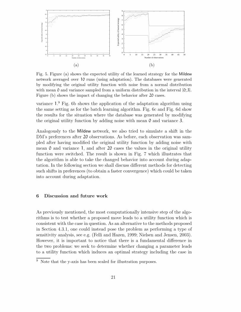
network averaged over 10 runs (using adaptation). The databases were generatedby modifying the original utility function with noise from a normal distributionwith mean 0 and variance sampled from a uniform distribution in the interval [0; 3].Figure (b) shows the impact of changing the behavior after 20 cases.
variance 1.9 Fig. 6b shows the application of the adaptation algorithm usingthe same setting as for the batch learning algorithm. Fig. 6c and Fig. 6d showthe results for the situation where the database was generated by modifyingthe original utility function by adding noise with mean 0 and variance 3.
Analogously to the Mildew network, we also tried to simulate a shift in theDM’s preferences after 20 observations. As before, each observation was sam-pled after having modified the original utility function by adding noise withmean 0 and variance 1, and after 20 cases the values in the original utilityfunction were switched. The result is shown in Fig. 7 which illustrates thatthe algorithm is able to take the changed behavior into account during adap-tation. In the following section we shall discuss different methods for detectingsuch shifts in preferences (to obtain a faster convergence) which could be takeninto account during adaptation.
6 Discussion and future work
As previously mentioned, the most computationally intensive step of the algo-rithms is to test whether a proposed move leads to a utility function which isconsistent with the case in question. As an alternative to the methods proposedin Section 4.3.1, one could instead pose the problem as performing a type ofsensitivity analysis, see e.g. (Felli and Hazen, 1999; Nielsen and Jensen, 2003).However, it is important to notice that there is a fundamental difference inthe two problems: we seek to determine whether changing a parameter leadsto a utility function which induces an optimal strategy including the case in
9 Note that the y-axis has been scaled for illustration purposes.
21

1.5
2
2.5
3
3.5
4
4.5
0 5 10 15 20 25 30 35 40 45 50
Exp
ecte
d ut
ility
of
lear
ned
stra
tegy
Number of observations
1.5
2
2.5
3
3.5
4
4.5
0 5 10 15 20 25 30 35 40 45 50
Exp
ecte
d ut
ility
of
lear
ned
stra
tegy
Number of observations
(a) (b)
1.5
2
2.5
3
3.5
4
4.5
0 5 10 15 20 25 30 35 40 45 50
Exp
ecte
d ut
ility
of
lear
ned
stra
tegy
Number of observations
1.5
2
2.5
3
3.5
4
4.5
0 5 10 15 20 25 30 35 40 45 50
Exp
ecte
d ut
ility
of
lear
ned
stra
tegy
Number of observations
(c) (d)
Fig. 6. The figures show the expected utility of the learned strategy for the Poker
network averaged over 10 runs; there are 186624 possible observation-decision se-quences. The two databases were generated by modifying the original utility functionwith noise from a normal distribution with mean 0 and variance 1. The results inFigure (a) were generated by the batch learning algorithm, and the results in Figure(b) were generated by the adaptation algorithm. Figure (c) and Figure (d) show theresults for the situation where the database was generated by modifying the originalutility function by adding noise with mean 0 and variance 3.
1.5
2
2.5
3
3.5
4
4.5
5
5.5
6
6.5
0 5 10 15 20 25 30 35 40 45 50
Exp
ecte
d ut
ility
of
lear
ned
stra
tegy
Number of observations
Fig. 7. The figure show the expected utility of the learned strategy for the Poker
network as a function of the number of cases (using adaptation); there are 186624possible observation-decision sequences. After 20 cases the values in the originalutility function were shifted to simulate a change in the DM’s preference. All obser-vations were generated by modifying the original utility function by adding noisewith mean 0 and variance 1.
22

question, whereas sensitivity analysis has to do with changes in the optimalstrategy. This also implies that the methods proposed in e.g. (Nielsen andJensen, 2003) cannot immediately be applied; these methods rely on the ex-pected utility functions being linear in the utilities, and this only holds whenthe optimal strategy is known (i.e., in our case, fully encoded in the database).
Thus, in order to apply the methods described by Nielsen and Jensen (2003)we could instead induce the “missing” cases: Start with the last decision, Dn,and determine the linear inequalities corresponding to each case by restrict-ing them to Dn, see Equation 6. Next, use these inequalities for checking theconstraints in step 3 of Algorithm 1 and determine a utility function for eachof the cases (again restricted to Dn). After the utility functions have beenfound we calculate an optimal policy for each case, and continue to decisionDn-1. Now, in order to compute the required inequalities for decision Dn-1(for a given case) we first substitute decision Dn with its chance variable rep-resentation (determined by the optimal policy induced by the utility functionidentified in the previous step), and decision Dn-1 is then treated as the lastdecision. This procedure then continues to the first decision variable, whereall unrestricted cases are considered.
Algorithm 2. Let D be a database consisting of N cases {c1, . . . , cN}, whereeach case specifies a realization of a strategy for the influence diagram I withdecision variables {D1, . . . , Dn} ordered by their indexes.
1. Set i := n.2. Repeat3. For each case c, calculate the expected value for all parameters ψcj .4. Use the estimated values to complete the optimal policy for decision Di in
each case.5. For each case substitute decision Di with its chance variable policy.6. Set i := i− 1.7. Until i = 0.
Note that as all the inequalities encode convex sets we are always workingwith a convex set during sampling; these sets are closed under intersection.Thus we can apply the sampling method proposed by Applegate and Kannan(1991).
An interesting approach for making the learning algorithm more robust, couldbe to weight the contribution from each case (i.e., changing the updating rulefor λj) in proportion to the probability of actually seeing that case. By weight-ing each case we can ensure that cases with low probability have less impact onthe learning procedure; this is consistent with their contribution to the maxi-mum expected utility. Moreover, by observing the “case probabilities” duringadaptation we could e.g. use the occurrence of low probability cases as an
23

indication of a shift in the DM’s preferences (producing a different behavior);thereby being able to change the value of λj accordingly and allowing a morerapid adaptation. Furthermore, it could be interesting to extend the proposedalgorithm to handle cases with missing values. One obvious approach to thisproblem would be to induce the missing data, however, it is not completelyapparent how these (partially induced) cases should be weighted as comparedto fully observed cases.
Finally, as also discussed in Section 3, we could base the learning methods on adescriptive model of the DM rather than a prescriptive. That is, acknowledgingthat humans rarely behave as to maximize the expected utility, we couldfor instance use the rank dependent utility (RDU) model by Quiggin (1982)during learning. In the RDU model, there are two parameters: i) a utilityfunction u(·) which is cardinal and represents the DM’s preferences undercertainty, and ii) a probability transformation (or weighting) function q(·),which is strictly increasing from [0, 1] onto itself. The utility V(L)u;q of asingle stage lottery L is determined as follows.10 First, the components of Lare re-indexed in increasing order of their utility:
L = (c1, p1; ...; ci, pi; ...; cn, pn) with u(c1) ≤ ... ≤ u(ci) ≤ ... ≤ u(cn).Then, its utility is evaluated as:
V(L)u;q =
n∑i=1 u(ci) q n∑j=i pj− q
n∑j=i+1pjor, equivalently as
V(L)u;q = u(c1) +
n∑i=2 [u(ci) − u(ci-1)]q n∑j=i pj .The crucial idea underlying the RDU model is that the utility of each con-sequence is given a variable weight, which depends on both its probabilityand on its ranking w.r.t. the other consequences of the lottery. The secondexpression suggests that the DM bases his evaluation on the probabilities ofachieving at least such or such utility level. Note, however, that RDU theoryno longer satisfies the independence axiom, and we cannot directly exploit theproperties of dynamic programming (Bellman, 1957) when dealing with se-quential decision problems. That is, the RDU model is computationally moreintensive to work with as compared to the EU model, and the integration ofthe model into the learning procedure is a subject for future research.
10 Note that under the reduction of compound lotteries assumption, any sequentialdecision problem can be transformed into a single stage lottery.
24

7 Conclusion
In this paper we have proposed two algorithms for learning a DM’s utilityfunction based on observed (possible inconsistent) behavior. The algorithmsextend previous proposed algorithms by explicitly taking into account thatthere may not exist a non-trivial utility function which can account for allthe observed behavioral patterns, i.e., behavior which jointly appear incon-sistent w.r.t. any utility function. The proposed algorithms are based on theassumption that inconsistent behavior can be explained as deviations froman underlying true utility function, and as such it can e.g. i) represent (orencode) inaccuracies in the model being applied (Shachter and Mandelbaum,1996), and ii) model a DM whose utility function fluctuates and/or changespermanently over time. The main difference in the two algorithms is that thefirst algorithm can be seen as a form of batch learning whereas the secondalgorithm focuses on adaptation. Empirical results demonstrated the applica-bility of both algorithms, which converged to the true utility function even forvery small databases. Additionally, it was shown that rapid permanent shiftsin the utility functions can also be taken into account during adaptation.
Acknowledgements
This paper has benefited from discussions with the members of the Deci-sion Support Systems group at Aalborg University, and in particular HelgeLangseth. We would also like to thank Hugin Expert (www.hugin.com) forgiving us access to the Hugin Decision Engine which forms the basis for ourimplementation. Finally, we would like to thank the anonymous reviewers fortheir constructive comments.
25

A Proofs
In order to estimate E(ψ∗j |D) we first note that:
P(ψ∗, σ2|D)
=
∫ c1 · · · ∫ cN P(ψ∗, σ2, ψc1, . . . , ψcN |D)dψc1 · · ·dψcN=
∫ c1 · · · ∫ cN P(ψ∗, σ2|ψc1, . . . , ψcN,D)P(ψc1, . . . , ψcN |D)dψc1 · · ·dψcN=
∫ c1 · · · ∫ cN P(ψ∗, σ2|ψc1, . . . , ψcN)P(ψc1, . . . , ψcN |D)dψc1 · · ·dψcN=
∫ 1 · · · ∫ m m∏j=1 P(ψ∗j , σ2j |ψc1j , . . . , ψcNj )
P(ψc1, . . . , ψcN |D)dψ1 · · ·dψm.(A.1)
In particular
P(ψ∗j , σ2j |D) =
∫ c1j · · ·
∫ cNj P(ψ∗j , σ2j |ψc1j , . . . , ψcNj )
P(ψc1j , . . . , ψcNj |D)dψc1j · · ·dψcNj(A.2)
In order to calculate the term P(ψ∗j , σ2j |ψc1j , . . . , ψcNj ) on closed form we needa conjugate prior distribution for the true utility function and the variance.First, recall that the conditional probability distribution for the utility pa-rameter ψcij of some case ci is a normal distribution which, for notationalconvenience, can be described in terms of its precision τj = 1/σ2j :
ψcij ∼ N(ψ∗j , τj) =
(
τj2π
)1=2exp
[
−1
2τj(ψcij − ψ∗j )2] . (A.3)
A possible conjugate family of joint prior distributions for ψ∗j (the mean) andτj (the precision), is the joint normal-gamma distribution specified by theconditional distribution of ψ∗j given τj and the marginal distribution of τj:
P(ψ∗j |τj, µ0j , λ0j ) =
(
λ0j τj2π
)1=2exp
[
−1
2λ0j τj(ψ∗j − µ0j )2]
P(τj|α0j , β0j ) =
(�0j )�0j�(�0j) τ�0j-1j e-�0j �j for τj > 00 for τj ≤ 0 (A.4)
26

for −∞ < µ0j < ∞, λ0j > 0, α0j > 0 and β0j > 0. That is, the conditionaldistribution of ψ∗j given τj is a normal distribution with mean µ0j and precisionλ0j τj, whereas the marginal distribution for τj is a gamma distribution withparameters α0j and β0j . Note that λ0j can be see as a virtual sample size, whichcan be used to control how certain we are about the distribution.
In the general case, suppose now that X1, X2, . . . , Xn form a random samplefrom a normal distribution for which both the mean µ and the precision τ areunknown. If the joint prior distribution of µ and τ is as specified above, thenthe joint posterior of µ and τ, given that Xi = xi (∀1 ≤ i ≤ n) is as follows:The conditional distribution of µ given τ is a normal distribution with meanµ1 and precision λ1τ, where:
µ1 =λ0µ0 + nxnλ0 + n
and λ1 = λ0 + n; (A.5)
xn is the sample mean, and the marginal distribution of τ is a gamma distri-bution with parameters α1 and β1:11
α1 = α0 +n
2and β1 = β0 +
1
2
n∑i=1 (xi − xn)2 +nλ0(xn − µ0)22(λ0 + n)
. (A.6)
In particular, we can find the expected value of µ (corresponding to the pa-
rameters of the true utility function) since E(µ) = µ1 and Var(µ) = �1�1(�1-1) .1211 Note also that when updating the prior distribution based on a random sampleof size n we also increase the virtual sample size λ0 with n.12 This is actually an approximation as the normal-gamma probability distributiononly serves as a conjugate prior for the unrestricted normal distribution and notwhen it is truncated.
27

Thus, we have:
E(ψ∗j |D)
=
∫ c1j · · ·
∫ cNj E(ψ∗j |ψc1j , . . . , ψcNj )P(ψc1j , . . . , ψcNj |D)dψc1j · · ·dψcNj=
∫ c1j · · ·
∫ cNj
λ0jµ0j +∑Ni=1ψcij
λ0j +N
P(ψc1j , . . . , ψcNj |D)dψc1j · · ·dψcNj=
λ0jµ0jλ0j +N
+1
λ0j +N
∫ c1j · · ·
∫ cNj N∑i=1 ψcij P(ψc1j , . . . , ψcNj |D)dψc1j · · ·dψcNj=
λ0jµ0jλ0j +N
+1
λ0j +N
N∑i=1 ∫ c1j · · ·
∫ cNj ψcij P(ψc1j , . . . , ψcNj |D)dψc1j · · ·dψcNj=
λ0jµ0jλ0j +N
+1
λ0j +N
N∑i=1 ∫ cij ψcij P(ψcij |D)dψcij .(A.7)
We shall approximate this expression by assuming that P(ψcij |D) ≈ P(ψcij |ci).The accuracy of this approximation is heavily dependent on the strength ofthe dependence between ψ∗k and ψcik as well as σ2k and ψckk ; with little priorknowledge encoded in the model these dependencies will be weak (encodedby a large variance or small λ). Given this assumption, E(ψ∗j |D) can now beexpressed as:
E(ψ∗j |D) ≈λ0jµ0jλ0j +N
+1
λ0j +N
N∑i=1 ∫ cij ψcij P(ψcij |ci)dψcij=
λ0jµ0jλ0j +N
+1
λ0j +N
N∑i=1 ψcij=λ0jµ0j +
∑Ni=1 ψcijλ0j +N
= E(ψ∗j |ψc1j , . . . , ψcNj ).
(A.8)
where ψci = E(ψci |ci).References
Allais, M., 1979. The foundation of a positive theory of choice involving riskand a criticism of the postulate and axioms of the american school. In:Expected utility hypotheses and the Allais paradox. Dordrecht, Holland,pp. 27–145, Original work published in 1952.
Applegate, D., Kannan, R., 1991. Sampling and integration of near log-concave
28
functions. In: Proceedings of the 23rd Annual ACM Symposium on Theoryand Computing. pp. 156–163.
Bellman, R. E., 1957. Dynamic Programming. Princeton University Press,Princeton.
Buntine, W. L., 1996. A guide to the literature on learning probabilistic net-works from data. IEEE Transactions on Knowledge and Data Engineering8, 195–210.
Chajewska, U., Getoor, L., Norman, J., Shahar, Y., 1998. Utility elicitationas a classification problem. In: Cooper, G. F., Moral, S. (Eds.), Proceedingsof the Fourteenth Conference on Uncertainty in Artificial Intelligence. pp.79–88.
Chajewska, U., Koller, D., 2000. Utilities as Random Variables: Density Es-timation and Structure Discovery. In: Boutilier, C., Goldszmidt, M. (Eds.),Proceedings of the Sixteenth Conference on Uncertainty in Artificial Intel-ligence. pp. 63–71.
Chajewska, U., Koller, D., Ormoneit, D., 2001. Learning an agent’s utilityfunction by observing behavior. In: Proceedings of the Eighteenth Interna-tional Conference on Machine Learning. pp. 35–42.
Chajewska, U., Koller, D., Parr, R., 2000. Making rational decisions usingadaptive utility elicitation. In: Proceedings of the Seventeenth National Con-ference on Artificial Intelligence. pp. 363–369.
Felli, J. C., Hazen, G. B., 1999. Sensitivity analysis and the expected value ofperfect information. Medical Decision Making 18, 95–109.
Howard, R. A., Matheson, J. E., 1981. Influence diagrams. In: Howard, R. A.,Matheson, J. E. (Eds.), The Principles and Applications of Decision Anal-ysis. Vol. 2. Strategic Decision Group, Ch. 37, pp. 721–762.
Jensen, F., Jensen, F. V., Dittmer, S. L., 1994. From Influence Diagramsto Junction Trees. In: de Mantaras, R. L., Poole, D. (Eds.), Proceedingsof the Tenth Conference on Uncertainty in Artificial Intelligence. MorganKaufmann Publishers, pp. 367–373.
Jensen, F. V., 2001. Bayesian networks and decision graphs. Springer-VerlagNew York, ISBN: 0-387-95259-4.
Johnson, N. L., Kotz, S., Balakrishnan, N., 1994. Continuous Univariate Dis-tributions, 2nd Edition. Vol. 1 of Wiley Series in Probability and Statistics.John Wiley and Sons, Inc.
Kahneman, D., Tversky, A., 1979. Prospect Theory: An Analysis of Decisionunder Risk. Econometrica 47, 263–291.
Keane, M. P., Wolpin, K. I., 1997. The career decisions of young men. Journalof Political Economy 105 (3), 473–522.
Lauritzen, S. L., Nilsson, D., 2001. Representing and solving decision problemswith limited information. Management Science 47 (9), 1235–1251.
Madsen, A. L., Jensen, F. V., 1999. Lazy evaluation of symmetric Bayesiandecision problems. In: Laskey, K. B., Prade, H. (Eds.), Proceedings of theFifthteenth Conference on Uncertainty in Artificial Intelligence. MorganKaufmann Publishers, pp. 382–390.
29

Ng, A. Y., Russell, S., 2000. Algorithms for inverse reinforcement learning.In: Proceedings of the Seventeenth International Conference on MachineLearning. pp. 663–670.
Nielsen, T. D., Jensen, F. V., 1999. Welldefined Decision Scenarios. In: Laskey,K. B., Prade, H. (Eds.), Proceedings of the Fifthteenth Conference on Uncer-tainty in Artificial Intelligence. Morgan Kaufmann Publishers, pp. 502–511.
Nielsen, T. D., Jensen, F. V., 2003. Sensitivity analysis in influence diagrams.IEEE Transactions on Systems, Man, and Cybernetics - Part A: Systemsand Humans 33 (2), 223–234.
Quiggin, J., 1982. A theory of anticipated utility. Journal of Economic Behav-ior and Organisation 3 (4), 323–343.
Rust, J., 1994. Structural estimation of Markov decision processes. In: Engle,R. F., McFadden, D. L. (Eds.), Handbook of Econometrics. Vol. IV. ElsevierScience B.V., pp. 3081–3143.
Sargent, T. J., 1978. Estimation of dynamic labor demand schedules underrational expectations. Journal of Political Economy 86 (6), 1009–1044.
Shachter, R. D., 1986. Evaluating Influence Diagrams. Operations ResearchSociety of America 34 (6), 79–90.
Shachter, R. D., 1999. Efficient value of information computation. In: Laskey,K. B., Prade, H. (Eds.), Proceedings of the Fifthteenth Conference on Uncer-tainty in Artificial Intelligence. Morgan Kaufmann Publishers, pp. 594–601.
Shachter, R. D., Mandelbaum, M., 1996. A measure of decision flexibility. In:Horvitz, E., Jensen, F. V. (Eds.), Proceedings of the Twelfth Conferenceon Uncertainty in Artificial Intelligence. Morgan Kaufmann Publishers, pp.485–491.
Suryadi, D., Gmytrasiewicz, P. J., 1999. Learning models of other agents usinginfluence diagrams. In: Preceedings of the Seventh International Conferenceon User Modeling. pp. 223–232.
Tatman, J. A., Shachter, R. D., 1990. Dynamic Programming and InfluenceDiagrams. IEEE Transactions on Systems, Man and Cybernetics 20 (2),365–379.
30