Embed Size (px)
Citation preview
1
LeakageLocalization
inWaterNetworks
Amodel‐basedmethodologyusing
pressuresensorsapplied
toarealcaseinBarcelonanetwork
Ramon Pérez*, Gerard Sanz, Vicenç Puig, Joseba Quevedo, Miquel À. Cugueró, Fatiha
Nejjari, Jordi Meseguer, Gabriela Cembrano, Josep M. Mirats, and Ramon Sarrate
*[email protected] +34937398620
September 18, 2013
The efficient use of water resources is a subject of major concern for water utilities and
authorities. One of the main challenges in improving the efficiency of drinking water networks
is to minimize water loss in pipes due to leakage. Water leaks in water distribution networks
(WDN) are unavoidable. They can cause significant economic losses in fluid transportation and
an increase on reparation costs that finally generate an extra cost for the final consumer due to
the waste of energy and chemicals in water treatment plants. It may also damage infrastructure
and cause third party damage and health risks. In many WDN, losses due to leakage are
estimated to account up to 30% of the total amount of extracted water; a very important issue in
a world struggling to satisfy water demands of a growing population.
Telemetry systems have long been used in large water distribution systems for
improving real-time monitoring of quantity and quality parameters. As monitoring technologies
2
evolve, new possibilities of controlling and managing complex infrastructures are provided.
This is the case for water networks. Sectorization of distribution networks into smaller
subnetworks, such as District Metered Areas (DMAs), contributes to achieving, in real-time, an
accurate estimation of the amount of water that is being consumed in each subnetwork. It is an
efficient measure to control water loss, since flow and pressure meters bring a huge amount of
data with information about the network behavior. Over the last decade, the concepts and
methods developed for system-wide water balance calculations have been based upon water
assets’ physical data and the statistics of pipe bursts, service connections and underground
conditions [1]. Performance measures and indicators are used to support the managerial
approaches to minimize different components of water losses.
Real-time monitoring of water networks is based on the use of sensor data from
telemetry and mathematical models to detect and diagnose possible abnormal situations, such as
leakage or water quality deterioration events. It links the real sensor data gathered from the
network to the decision making procedure, by detecting possible faults as well as their probable
location within the network. The main idea behind real-time monitoring, both for water balance
and for water quality problems, is to use real-time sensor data and to compare them with those
generated by a well-calibrated hydraulic model of the network in absence of faults. By
analyzing the difference between these two sets of data, a detection of abnormal events can be
performed.
Several works have been published on leak detection and isolation methods for WDN.
For example, a review of transient-based leak detection methods is offered in [2] as a summary
of current and past work. In [3], a method has been proposed to identify leaks using blind spots
based on previously leak detection researches that use the analysis of acoustic and vibrations
signals [4], and models of buried pipelines to predict wave velocities [5]. More recently, a
method to locate leaks using Support Vector Machines (SVM) has been developed in [6]. The
3
approach analyses data obtained by a set of pressure control sensors of a pipeline network to
locate and calculate the size of the leak.
Another set of methods is based on the inverse transient analysis [7, 8]. The main idea
of this methodology is to analyze the pressure data collected during the occurrence of transitory
events by means of the minimization of the difference between the observed and the calculated
parameters. It is shown in [9, 10] that unsteady-state tests can be used for pipe diagnosis and
leak detection. The transient-test based methodologies are used exploiting the equations for
transient flow in pressurized pipes in frequency domain and in the second part, information
about pressure waves is taken into account.
Model based leak detection and isolation techniques have also been studied. In [11], the
leak detection and location problem is formulated as a least-squares estimation problem.
However, the parameter estimation of non-linear models of water networks is not an easy task
due to the fact that in most of the cases the problem is underdetermined because of the quantity
of pressure measurements. Alternatively, in [12, 13], a method based on pressure measurements
and leak sensitivity analysis is proposed. This methodology consists in analyzing the residuals
(difference between the measurements and their estimation using the network hydraulic model)
on-line regarding a given threshold that takes into account modeling uncertainty and noise.
When some of the residuals exceed their threshold, they are compared against the leak
sensitivity matrix in order to discover which possible leak is present. Although this approach
has good efficiency under ideal conditions, its performance decreases due to the nodal demand
uncertainty and noise in the measurements. In case that flow measurements are available, leaks
could be more easily detected since simple mass balance in the pipes can be established. See for
example [14] where a methodology to isolate leaks is proposed using fuzzy analysis of the
residuals. This method computes the residuals between the nominal measurements (that is,
without leak) and the measurements with leaks. However, although the use of flow
measurements is viable in large water transport networks this is not the case in water
4
distribution networks where there is a dense mesh of pipes with only flow measurements at the
entrance of each DMA. In this situation, water companies suggest as a feasible solution to
install some pressure sensors inside the DMA. Pressure sensors in this situation are preferred
because they are cheaper and easy to install and maintain.
The article describes a model-based methodology for leakage detection and localisation
in DMAs of water distribution networks, based on the use of pressure sensors. This
methodology is founded in the principles of model-based diagnosis [15, 16], but enhancing fault
isolation using residual fault sensitivity analysis instead of using the standard binary fault
signature approach extending the preliminary results presented in [12, 13]. This methodology
has been developed as a part of a cooperative project between the Advanced Control Systems
Group of the Technical University of Catalonia (SAC-UPC), Cetaqua (Water Technology
Centre, Barcelona, Spain), Ondéo Systems S.A. (Le Pecq, Region Parisienne, France) and
SAFEGE (Paris, France). The methodology has been implemented in a general software tool
that interfaces with a GIS system being useful for a large class of water distribution systems and
has been successfully tested in a real implementation in a DMA of Barcelona, Spain.
The main concepts of the methodology are described first. The software tool is
presented followed by the results of the real application. Finally, conclusions and an outline of
on-going and future further research are provided.
Methodology
The standard theory of model based diagnosis includes two steps [15]. First of all, fault
detection uses consistency checking for signaling the existence of a fault. Once the fault is
detected, isolation is carried out based on observed fault signatures, generated by the detection
module, and its relation with the theoretical fault signature matrix obtained from the structural
analysis of the model [16]. Leak localization techniques based on analytical models [13] can be
seen as an application of fault detection and isolation techniques developed by complex

5
industrial systems. In this case, the analyzed system is a DMA water network and, the potential
faults are those leaks affecting the network components (that is, pipes). However, standard tools
used in model based fault diagnosis should be adapted because the model of a DMA is given by
a set of non-linear equations highly coupled and without an explicit solution.
This application is developed thinking on real water distribution networks with
kilometers of pipes. The consistency between measurements and model prediction is always
difficult to achieve because of model uncertainty, especially in the nodal demands that usually
are estimated. Thus, the detection phase is usually treated in another level of supervision using
DMA information regarding night flows and water balance performance (see [17] for further
details).
Leakage monitoring may be performed on a routine basis or when major losses are
suspected [18]. Technologies for locating leaks range from ground-penetrating radar to acoustic
listening devices [19]. Some of these techniques require isolating and shutting down part of the
network. Techniques based on locating leaks from pressure monitoring devices allow a more
effective and less costly search in situ. This article proposes a leak localization method based
on the pressure measurements and pressure sensitivity analysis of nodes in a network when a
leak is present.
When leaks are sought, the number of possible places where they can be located is
infinite. However, it is a common practice to assume that leaks are in any of the network
junctions so the number of possible faults remains huge but becomes finite and the
approximation is irrelevant taking into account the size of the system [11].
The development of the methodology started with the work presented in [13]. In this
methodology, the sensor placement is a previous step that allows selecting the places for
pressure sensors so that the cardinal of the biggest group of discriminated leaks is minimal [12].
The main drawback of this first version of the methodology lies on the threshold selection for
the binarization of the leak sensitivity matrix in order to apply the standard fault isolation theory
6
[15, 16]. The comparison of residuals with the sensitivity to a leak using correlation improves
the results [20], since correlation avoids binarization. First simulation results based on this
methodology are presented in [21]. The improved results obtained using correlation justify the
use of this approach for the real pilot tests, as will be shown in this work.
Methodology step by step
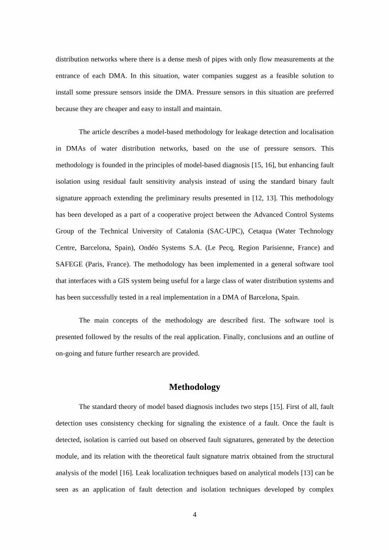
The zone with the highest leak probability can be determined online in the following six
step iterative procedure:
1. Simulation of possible faults in the different nodes of the network using
a hydraulic simulation (EPANET in this work)
2. Generation of the sensitivity-to-leak matrix containing the theoretical
Fault Signature Matrix (FSM) [15] of all considered potential leaks.
3. Collecting pressure measurements from sensors installed in the
network.
4. Generation of residuals comparing pressure measurements with
estimations provided by the hydraulic simulator, considering a model without leakage.
5. Comparison of residuals with the FSM contained in the sensitivity-to-
leak matrix using the correlation function.
6. Results aggregation and representation.
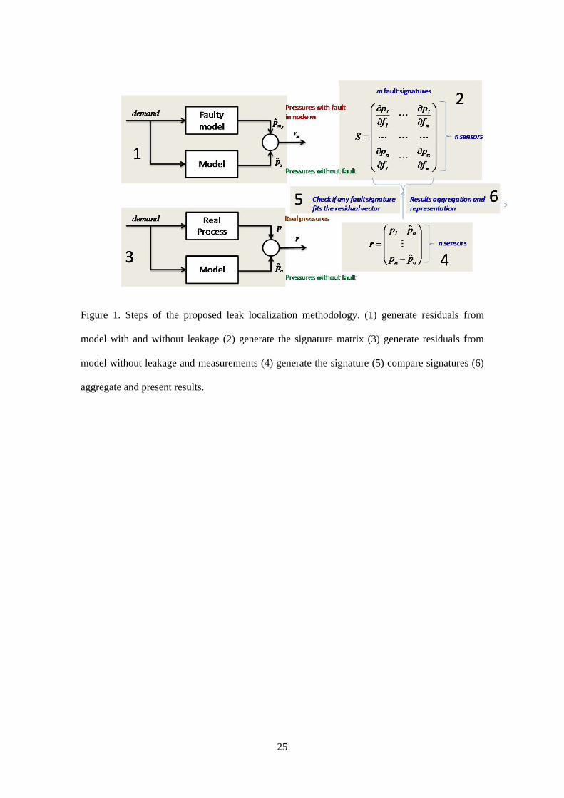
Figure 1 shows the iterative process searching nodes whose leakage signature has
maximal likelihood with the residual obtained from measurements.
Simulation of possible faults
The first step is to generate the model of all the possible leaks that may exist in the
network. A size of leakage has to be assumed or estimated. The residual sensitivity-to-leak
matrix (FSM) and the observed signatures (residuals) depend on the leakage size; nevertheless
the correlation method is robust to bad estimations of the leakage size [21]. The model is
7
simulated with the boundary conditions (global demand and boundary pressures) at any time-
step and the pressures obtained at the nodes where sensors are present are saved ( ̂ ). Then,
placing a leak at a certain node and running as many simulations as considered potential leaks
(number of nodes), pressures for each scenario are saved ( ̂ ).
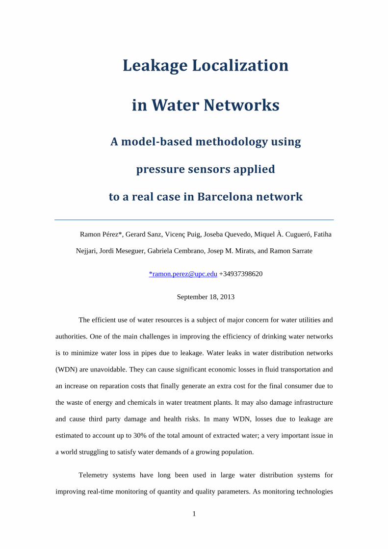
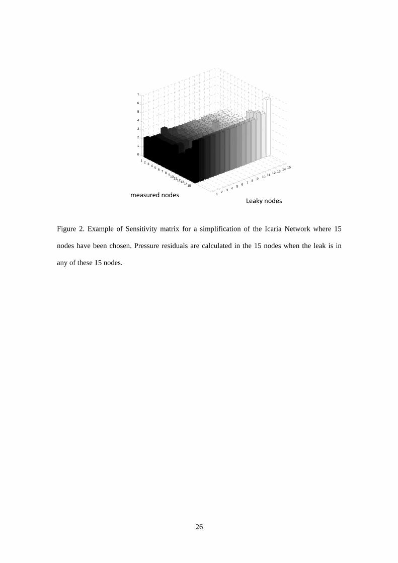
Generation of Sensitivity Matrix (FSM)
The difference between the pressure simulated without leakage and the pressure
simulated with each leak gives the theoretical signature for each possible leak and for a given
size. It is an approximation of the residual sensitivity-to-leak matrix [11]
.. . .
.
.. . .
.,
where m is the number of possible leak locations, f is the assumed leak size, and n is the number
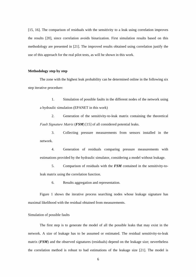
of sensors. Figure 2 shows the result for a small network with only 15 nodes and with a sensor
in each node for illustrative purposes.
Notice that this Sensitivity Matrix depends on the magnitude of the leakage because the
equations of the network are nonlinear. In particular, the non-linearity appears because pressure
and flow in a pipe are related through the Hanzen-Williams equation
∆ . ,
where R is the pipe roughness.
Measurement at the network
Pressure measurements within the network are used. This kind of sensor is
recommended by the company because of its reliability and cost compared with flow sensors.
Nevertheless, the accuracy of the installed sensors is 10 cm and in simulation, leaks of interest,
8
smaller than 10 l/s, produced pressure differences often smaller than 10 cm. Besides, sensor
noise requires filtering.
Resolution may be enhanced using oversampling [22]. The idea is to use the mean of t
measurements provided in an iteration time T (in this work the iterations are each hour and
sampling time is 10 minutes thus the mean is over 6 values). This mean operation filters the
noise of high frequency and leads to a better resolution than the sensors (10 cm in this network).
Pressures generated by simulation are truncated to the first decimal and the mean is calculated
so that the information containing is equivalent to that provided by the measurements.
Generation of the residuals
Estimated pressures without leakage are subtracted from the mean of pressure
measurements in T obtaining the residuals
∑ ̂⋮
∑ ̂,
where index j indicates the ordinal of measurements in an hour and k the index related to a given
hour.
Comparison of residuals with the theoretical fault signatures (FSM)
Residuals at time k are compared with all columns ( of the leak sensitivity matrix S
that correspond with the potential leaks to be isolated. This comparison is obtained applying the
Pearson’s correlation coefficient , between two variables , that is defined as
, cov , r cov , cov r, r⁄ ,
where cov , is the covariance function between two variables a and
b, being and ,respectively. The columns of S (possible node leaks) having
bigger correlation values with the residual vector at time k are the most probable nodes to have a
9
leak. The correlation between the observed residual fault signature (that is r(k)) and each
column of the matrix S(k) (that is for fault , considering I possible faults) is a measure of
the similarity between the leak residual effect (with unknown magnitude) and the leaks
considered in the matrix S (with known magnitude) that allows discovering which is the column
of this matrix (fault) having the same behavior.
For linear systems the correlation function obtains the maximum similarity, that is ρ=1,
in the node having the leak for any magnitude of this leakage. Because of the non-linearity of
the water network system, if the magnitude of the leakage is far from the one used to compute
the sensitivity matrix S, the similarity of the correlation function decreases but a high
correlation between the residuals corresponding to a particular leak and the corresponding
column of this matrix still exists.
Results aggregation and representation
The simulation model of the studied DMA mainly contains pipes and junctions. If tanks
were considered the methodology would not be much affected as the level of tanks is usually
monitored. Length, diameter and roughness of pipes are parameters with rather confidence.
Nevertheless demands are a very uncertain parameter. A study of the effect of a bad calibration
in demands on the leakage localization [23] showed that these parameters are critical since
demands and leakages behave exactly the same. The spatial distribution of demands was revised
using the registered water of last months. Once real pressure is used another critical point is a
good determination of the topographical head associated with every monitored node. Before the
real test was carried out the topographical heads had to be revised because the approximate data
were not accurate enough taking into account the pressure differences that leakages produce.
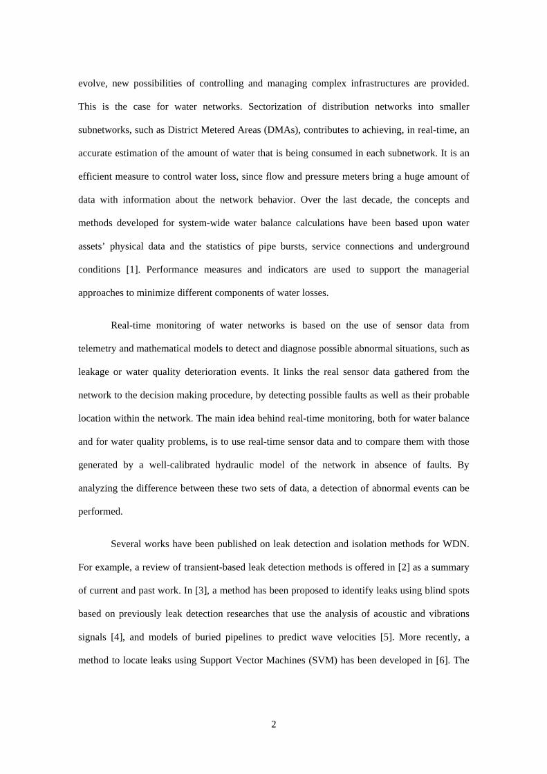
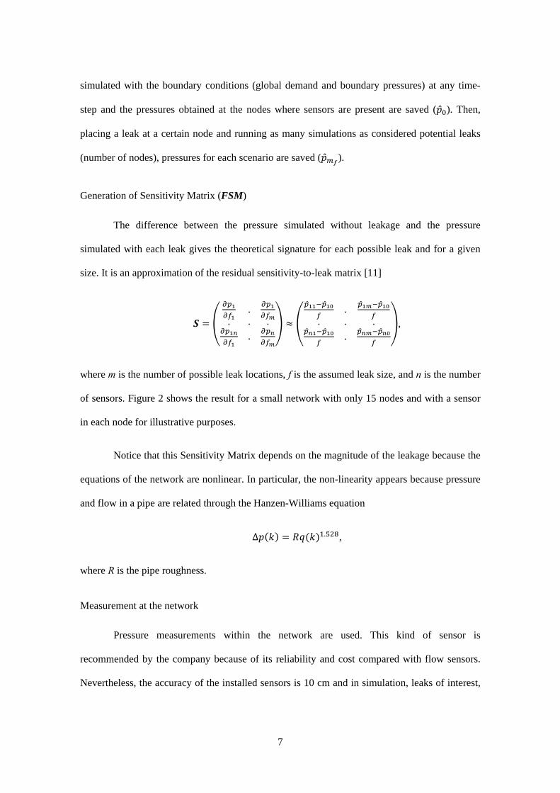
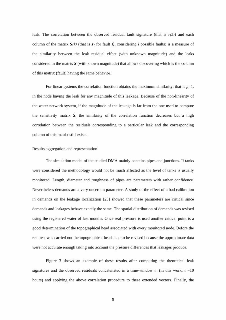
Figure 3 shows an example of these results after computing the theoretical leak
signatures and the observed residuals concatenated in a time-window τ (in this work, τ =10
hours) and applying the above correlation procedure to these extended vectors. Finally, the
10
representation is done by means of a grey scale for each node, being those with a higher score a
darker representation
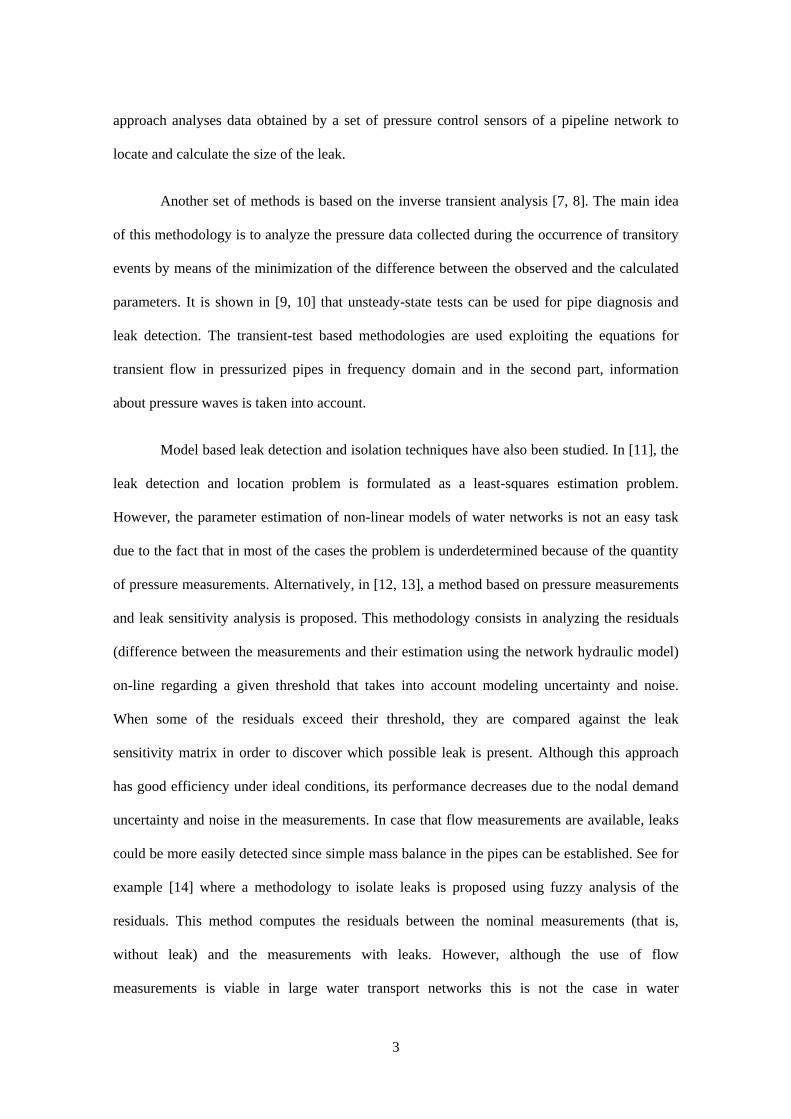
Software
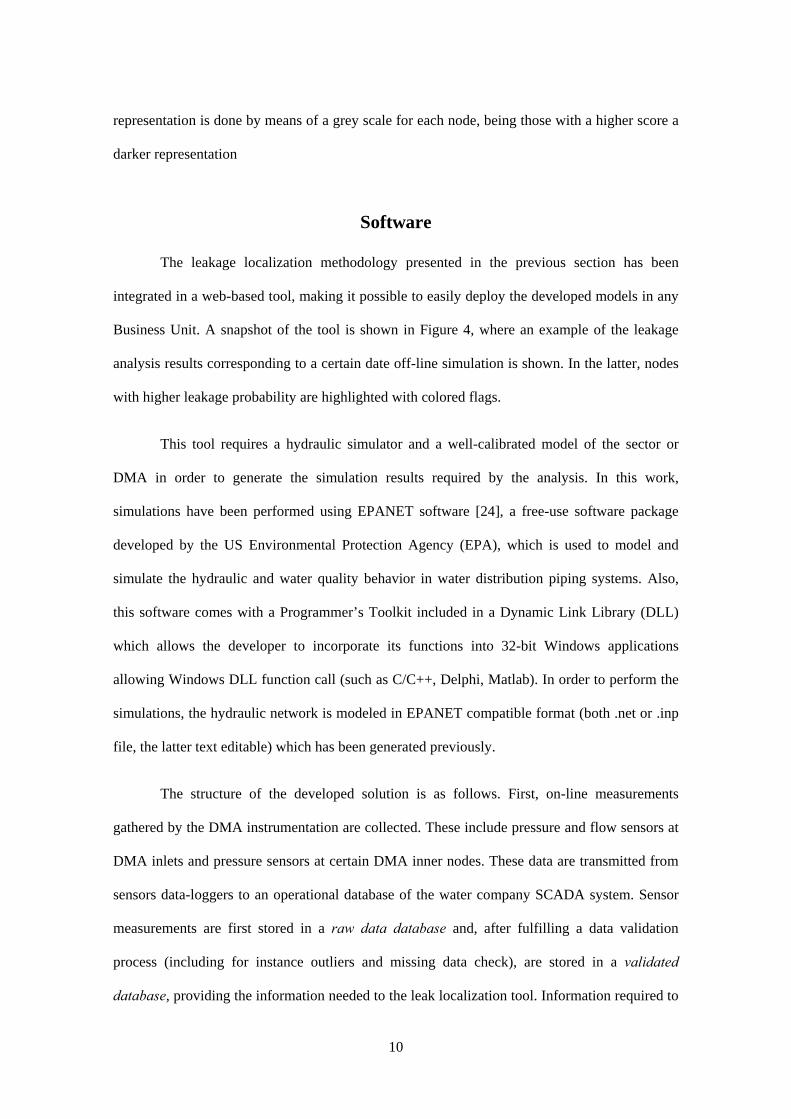
The leakage localization methodology presented in the previous section has been
integrated in a web-based tool, making it possible to easily deploy the developed models in any
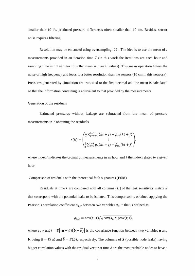
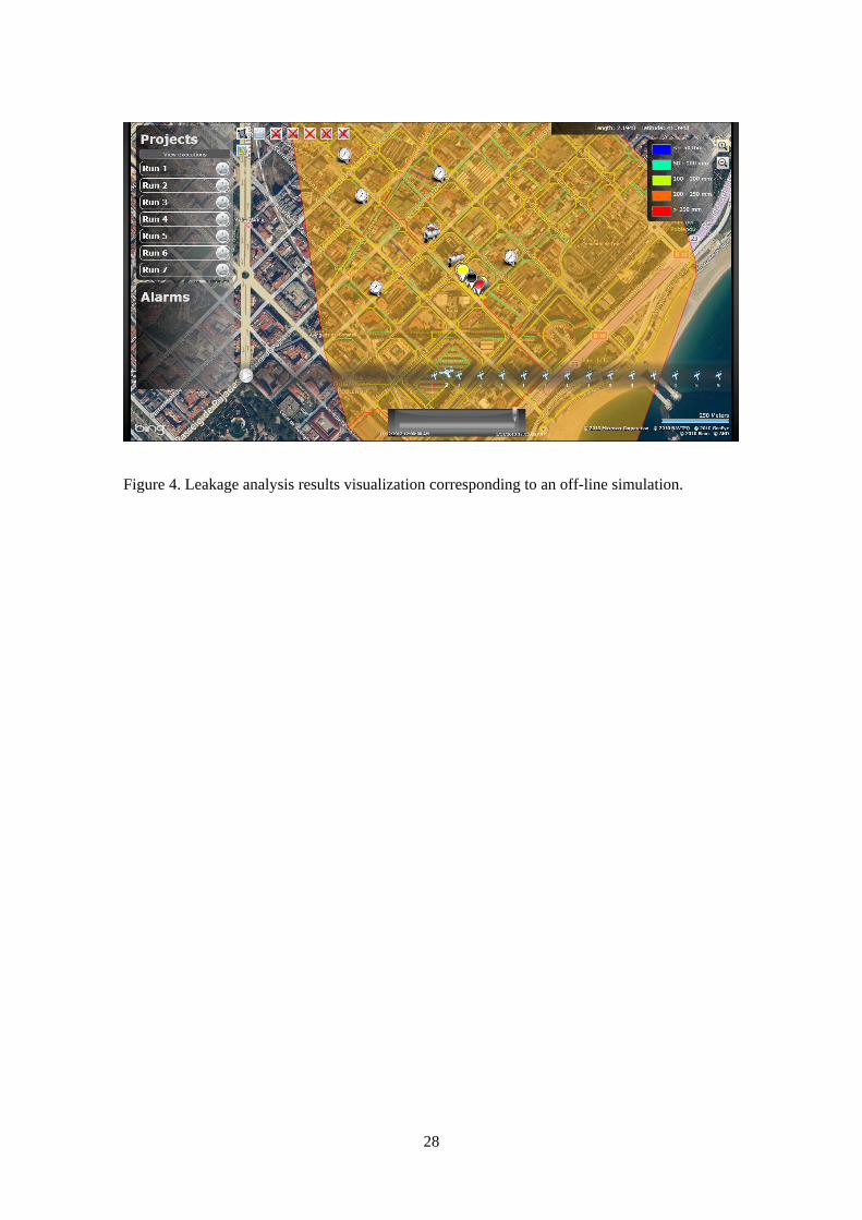
Business Unit. A snapshot of the tool is shown in Figure 4, where an example of the leakage
analysis results corresponding to a certain date off-line simulation is shown. In the latter, nodes
with higher leakage probability are highlighted with colored flags.
This tool requires a hydraulic simulator and a well-calibrated model of the sector or
DMA in order to generate the simulation results required by the analysis. In this work,
simulations have been performed using EPANET software [24], a free-use software package
developed by the US Environmental Protection Agency (EPA), which is used to model and
simulate the hydraulic and water quality behavior in water distribution piping systems. Also,
this software comes with a Programmer’s Toolkit included in a Dynamic Link Library (DLL)
which allows the developer to incorporate its functions into 32-bit Windows applications
allowing Windows DLL function call (such as C/C++, Delphi, Matlab). In order to perform the
simulations, the hydraulic network is modeled in EPANET compatible format (both .net or .inp
file, the latter text editable) which has been generated previously.
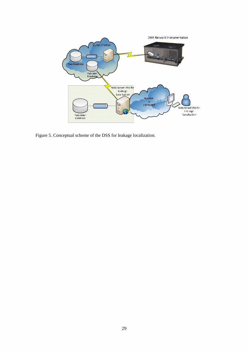
The structure of the developed solution is as follows. First, on-line measurements
gathered by the DMA instrumentation are collected. These include pressure and flow sensors at
DMA inlets and pressure sensors at certain DMA inner nodes. These data are transmitted from
sensors data-loggers to an operational database of the water company SCADA system. Sensor
measurements are first stored in a raw data database and, after fulfilling a data validation
process (including for instance outliers and missing data check), are stored in a validated
database, providing the information needed to the leak localization tool. Information required to
11
construct the EPANET model of the DMA network (for instance topological structure,
roughness, length and diameter for pipes, location of sensors, demand patterns) is obtained from
a parameters database. Finally, either on-line or manually (that is, specifying a range of dates)
leak localization analysis is performed and results are presented to the network operator as
depicted in Figure 4. Figure 5 provides a general scheme of the presented structure.
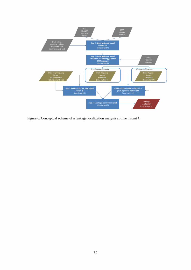
Moreover, a conceptual diagram showing the leakage localization analysis procedure at
a certain time instant k is provided in Figure 6.
The several steps involved in the method in Figure 6 are described next
Step 1 - Calibration of the DMA hydraulic model. The process involved in step 1 needs
the following inputs: the DMA hydraulic model (in EPANET format), the pressure and flow
measurements in the DMA inlets between k and k-1 time instants, the base demand values of the
DMA inner nodes and the value of the demand patterns at time instant k. The output is a
calibrated model of the DMA hydraulic network at time instant k, the latter used to predict
pressure and flow values at the DMA inlets and pressure in monitored inner nodes.
Step 2 - DMA hydraulic model simulation considering potential DMA leakages. This
process needs the calibrated DMA hydraulic model at time instant k obtained in Step 1 and the
locations of the potential leakages that may appear in the DMA. Step 2 follows an iterative
process running as many iterations as considered potential leakages. For every potential leak, its
effect on the pressure values of the monitored DMA inner nodes is estimated.
Step 3 – Computing the fault signal vector (k) (i.e. residuals r(k)). To proceed with
step 3, the pressure sensor measurements between time instant k and k-1 at the monitored DMA
inner nodes as well as the estimated pressure using the calibrated DMA hydraulic model,
assuming a faultless (that is, leakage-free) scenario, are needed. The output is the residual vector
r(k) (or fault signal vector (k)), that is, a vector of pressure differences between the pressure
12
measured by ith sensor and the predicted pressure value associated with ith pressure sensor in a
faultless scenario.
Step 4 – Computing the theoretical fault signature matrix FSM(k) (i.e. sensitivity
matrix S(k)). To perform this step, the pressure estimation at time instant k in all the monitored
nodes considering all DMA potential leaks (Step 2), as well as its pressure estimation at time
instant k using the calibrated DMA faultless hydraulic model (Step 1), is needed. The pressure
differences in the monitored DMA nodes between the faultless scenario and each leakage
scenario is obtained in order to compute the matrix FSM(k) (S(k)).
Step 5 – Leak localization result. This last step provides the most probable localizations
of the potential existing leakages. This result is obtained for k ≥ τ (time accumulation window),
considering the τ-past values of r(k) ((k)) (obtained in Step 3) and S(k) (FSM(k)) (obtained in
Step 4).
See [25] for further details on the software implementation.
Results
Description of Nova Icaria District Metered Area (DMA)
This model-based leakage localization methodology has been tested in one DMA of
Barcelona under a real leakage scenario. The water network which contains this DMA supplies
both Barcelona and its metropolitan area covering around 3 million of inhabitants and is
managed by the water company SGAB. The whole water network is composed by 4.574 km of
pipes, 65 pumping stations and 72 water tanks with a water storage capacity up to 250.542 m3.
This network is segmented into 117 pressure levels and 214 District Metered Areas (DMAs). In
this pilot implementation, the Barcelona’s DMA of Nova Icaria has been used. It is included in
level 55 within the city network, and has two inlets (Alaba and Llull), 3377 nodes and 3442
13
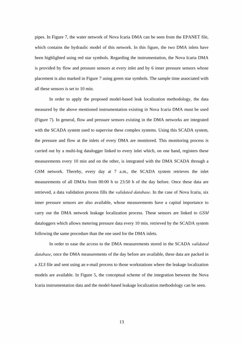
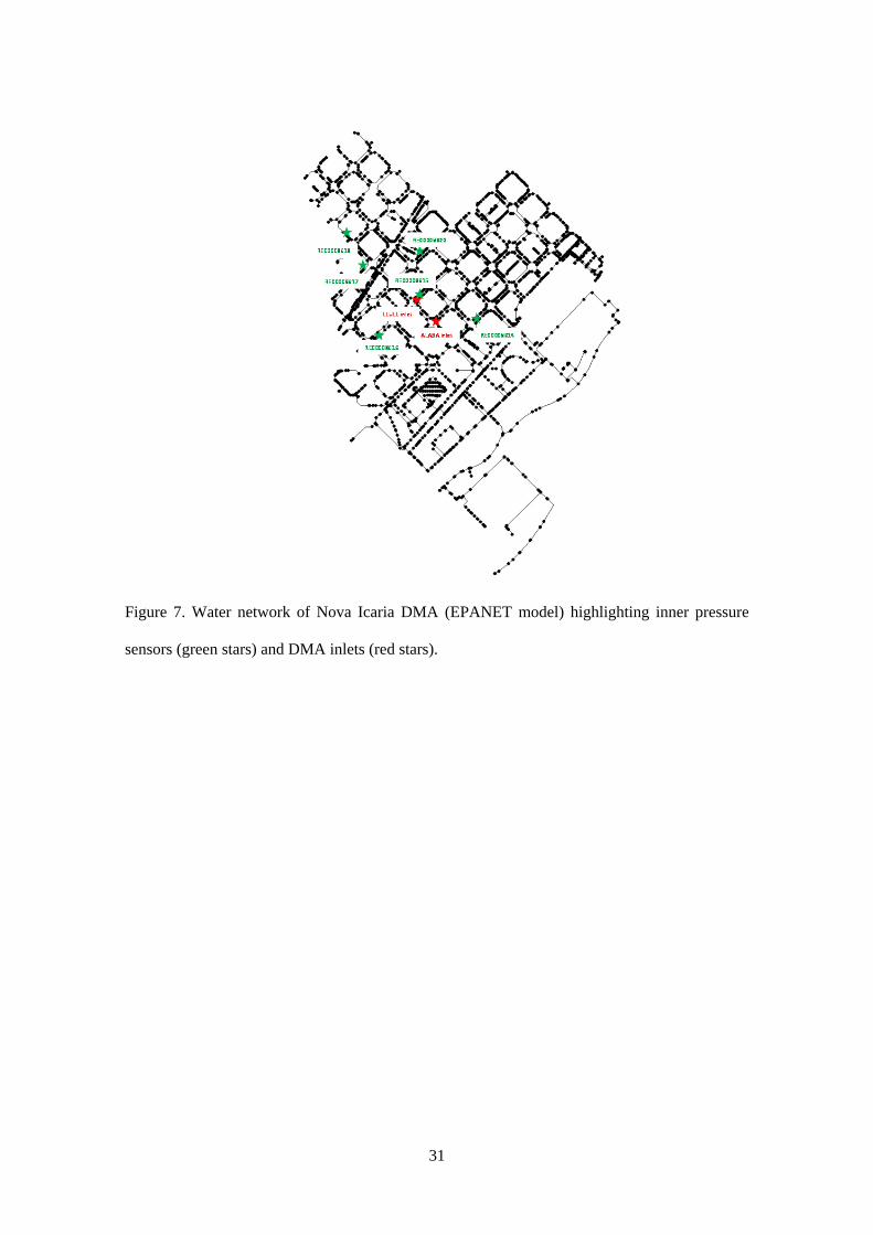
pipes. In Figure 7, the water network of Nova Icaria DMA can be seen from the EPANET file,
which contains the hydraulic model of this network. In this figure, the two DMA inlets have
been highlighted using red star symbols. Regarding the instrumentation, the Nova Icaria DMA
is provided by flow and pressure sensors at every inlet and by 6 inner pressure sensors whose
placement is also marked in Figure 7 using green star symbols. The sample time associated with
all these sensors is set to 10 min.
In order to apply the proposed model-based leak localization methodology, the data
measured by the above mentioned instrumentation existing in Nova Icaria DMA must be used
(Figure 7). In general, flow and pressure sensors existing in the DMA networks are integrated
with the SCADA system used to supervise these complex systems. Using this SCADA system,
the pressure and flow at the inlets of every DMA are monitored. This monitoring process is
carried out by a multi-log datalogger linked to every inlet which, on one hand, registers these
measurements every 10 min and on the other, is integrated with the DMA SCADA through a
GSM network. Thereby, every day at 7 a.m., the SCADA system retrieves the inlet
measurements of all DMAs from 00:00 h to 23:50 h of the day before. Once these data are
retrieved, a data validation process fills the validated database. In the case of Nova Icaria, six
inner pressure sensors are also available, whose measurements have a capital importance to
carry out the DMA network leakage localization process. These sensors are linked to GSM
dataloggers which allows metering pressure data every 10 min, retrieved by the SCADA system
following the same procedure than the one used for the DMA inlets.
In order to ease the access to the DMA measurements stored in the SCADA validated
database, once the DMA measurements of the day before are available, these data are packed in
a XLS file and sent using an e-mail process to those workstations where the leakage localization
models are available. In Figure 5, the conceptual scheme of the integration between the Nova
Icaria instrumentation data and the model-based leakage localization methodology can be seen.
14
Leakage Scenario in Nova Icaria
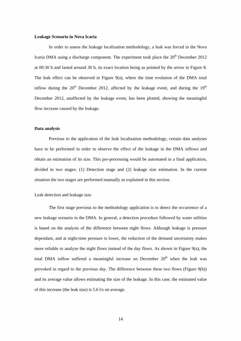
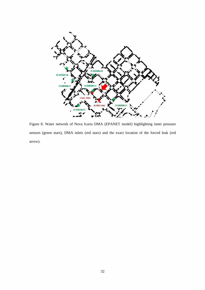
In order to assess the leakage localization methodology, a leak was forced in the Nova
Icaria DMA using a discharge component. The experiment took place the 20th December 2012
at 00:30 h and lasted around 30 h, its exact location being as pointed by the arrow in Figure 8.
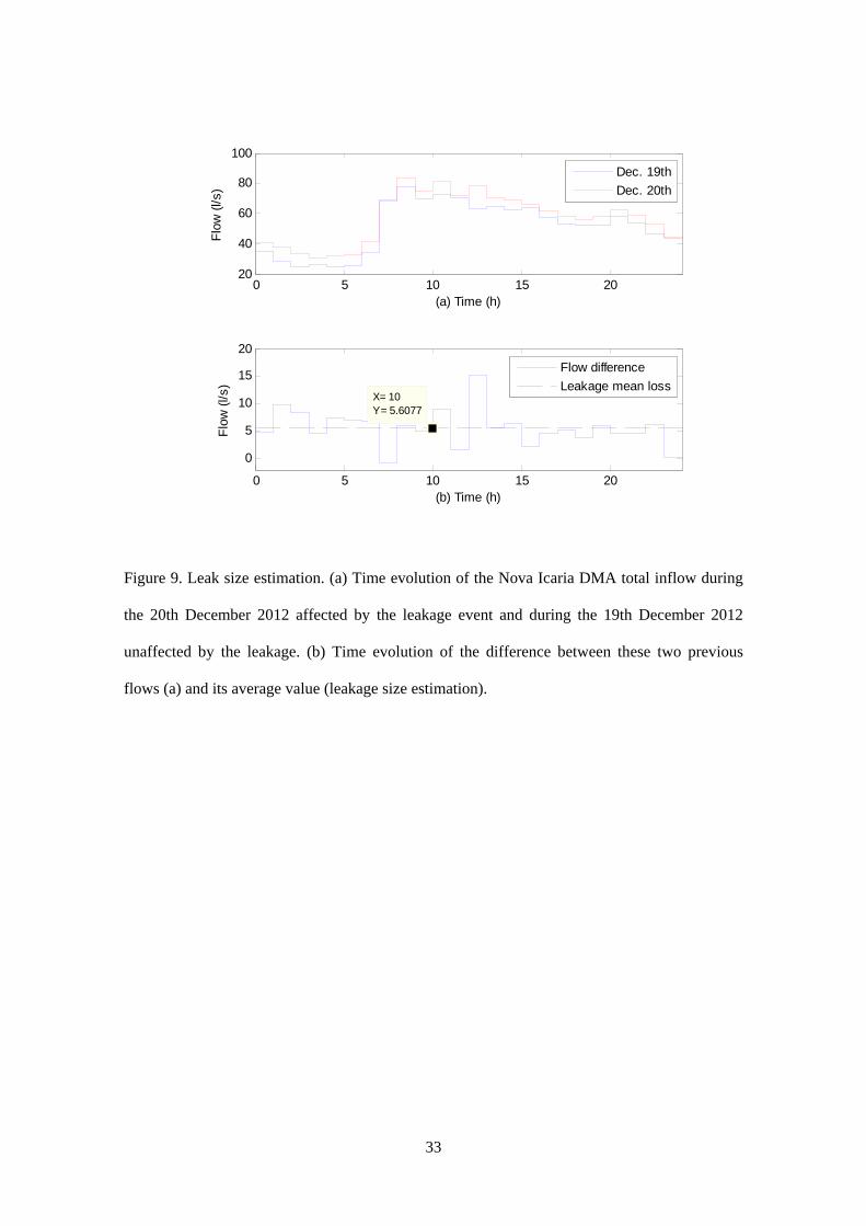
The leak effect can be observed in Figure 9(a), where the time evolution of the DMA total
inflow during the 20th December 2012, affected by the leakage event, and during the 19th
December 2012, unaffected by the leakage event, has been plotted, showing the meaningful
flow increase caused by the leakage.
Data analysis
Previous to the application of the leak localization methodology, certain data analyses
have to be performed in order to observe the effect of the leakage in the DMA inflows and
obtain an estimation of its size. This pre-processing would be automated in a final application,
divided in two stages: (1) Detection stage and (2) leakage size estimation. In the current
situation the two stages are performed manually as explained in this section.
Leak detection and leakage size
The first stage previous to the methodology application is to detect the occurrence of a
new leakage scenario in the DMA. In general, a detection procedure followed by water utilities
is based on the analysis of the difference between night flows. Although leakage is pressure
dependant, and at night-time pressure is lower, the reduction of the demand uncertainty makes
more reliable to analyze the night flows instead of the day flows. As shown in Figure 9(a), the
total DMA inflow suffered a meaningful increase on December 20th when the leak was
provoked in regard to the previous day. The difference between these two flows (Figure 9(b))
and its average value allows estimating the size of the leakage. In this case, the estimated value
of this increase (the leak size) is 5.6 l/s on average.

15
Regarding the leakage simulation in water network models, in general leaks are not
simulated as constant consumptions. It is more realistic to set an emitter coefficient in a node
which will generate a leakage size depending on the pressure of that node [24]
q Cp , (0)
where q is the leak size; C is the emitter coefficient provided; p is the pressure at the node; and γ
is an exponent in the range of 0.5 (Hazen-Williams, Darcy-Weisbach, Chezy-Manning
formulas).
The model-based leakage localization methodology requires the estimation of the
emitter coefficient C which according to Equation (0) can be obtained using the estimated
average size of the leakage (5.6 l/s, Figure 9(b)) and an estimation of the average pressure in the
leakage localization. This average pressure has been estimated averaging the measurements of
the DMA inner pressure sensors for the 20th December (leakage scenario shown in Figure 11)
which is around 50 m.w.c. (meter of water column). As a result, and using γ=0.5 (Darcy-
Weisbach formula), the estimated emitter coefficient is 0.8. The peaks in the leakage observed
in Figure 9 will be modulated by the network pressure.
Calibration: DMA hydraulic model and inner pressure sensor
The last stage before launching the leak isolation methodology is to verify the
calibration of the DMA hydraulic model and the inner pressure sensors since existing model
errors or poor calibrations may lead to a low-confident performance of the leakage isolation
methodology. In order to carry out this process, the data of December 19th have been used since
no major leaks were present that day. The general procedure to calibrate the DMA hydraulic
model derives from the one proposed in [21] where the pressure in the DMA inlets at time
instant k is set while the flow value in the inlets at this time instant is distributed among all the
DMA inner nodes according to the values of their base demand and related demand patterns. As
pointed out in [26], the DMA water demand model (that is, base demand of nodes and their
demand patterns) is one of the main sources of uncertainty which may lead to inaccurate
16
performances and consequently, a special attention should be paid in their calibration. In the
application considered in this article, the base demand of the network nodes and their demand
pattern (water demand model) have been obtained through a basic process using the billing
information of this DMA offered by SGAB. As an output of the whole model calibration
process, a calibrated model of the DMA hydraulic network at every time instant k is obtained
which can be used to predict the pressure and flow values in the DMA inlets and the pressure in
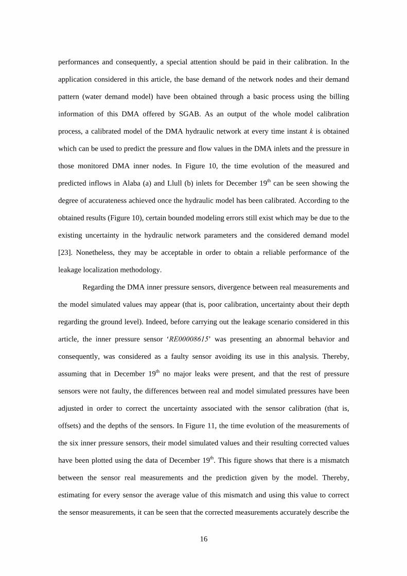
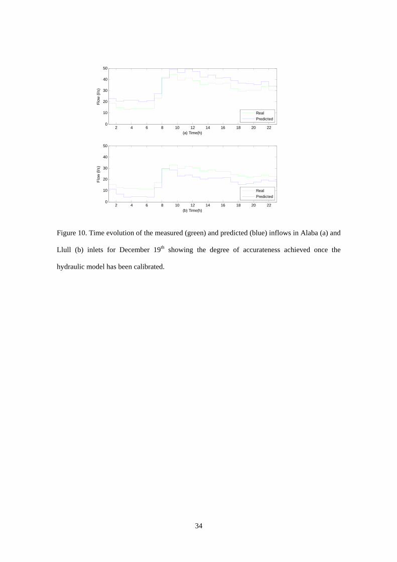
those monitored DMA inner nodes. In Figure 10, the time evolution of the measured and
predicted inflows in Alaba (a) and Llull (b) inlets for December 19th can be seen showing the
degree of accurateness achieved once the hydraulic model has been calibrated. According to the
obtained results (Figure 10), certain bounded modeling errors still exist which may be due to the
existing uncertainty in the hydraulic network parameters and the considered demand model
[23]. Nonetheless, they may be acceptable in order to obtain a reliable performance of the
leakage localization methodology.
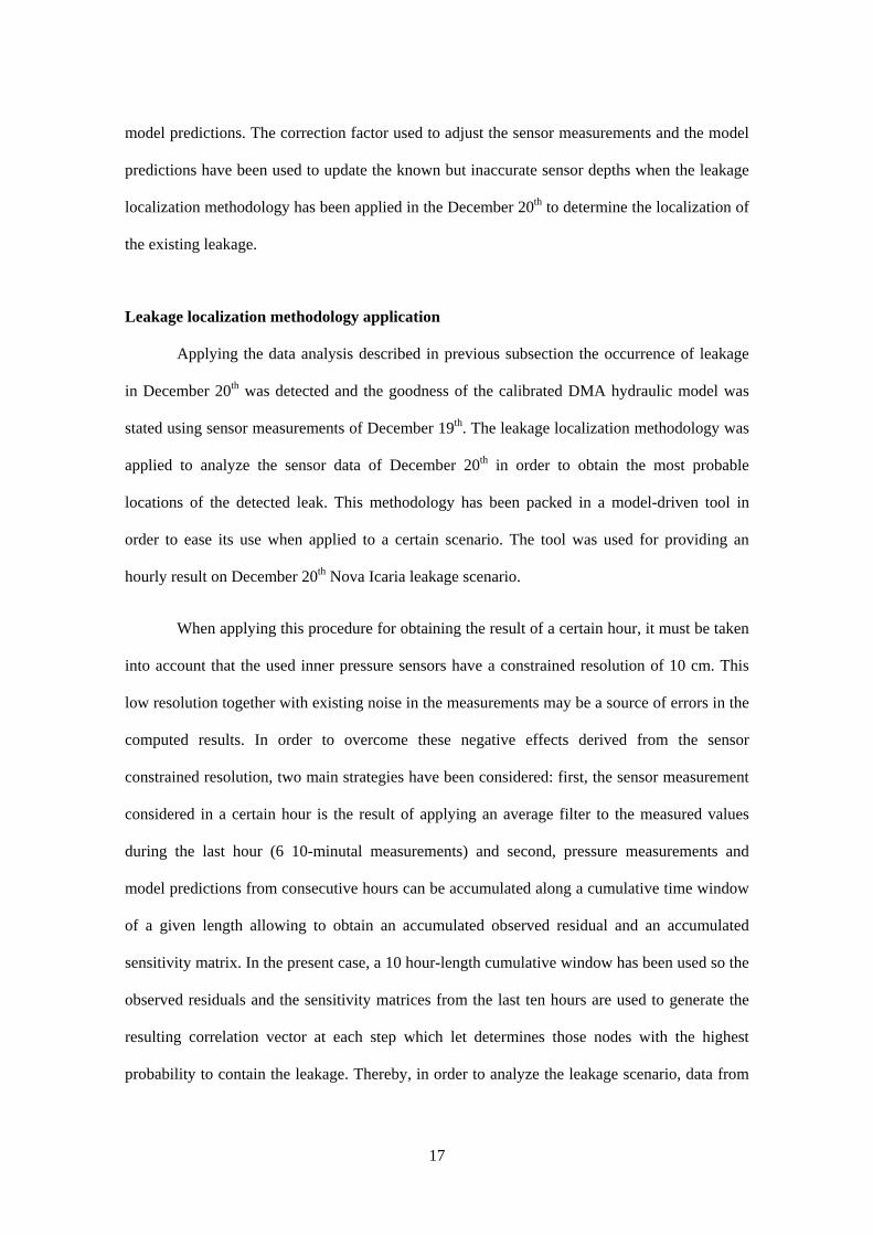
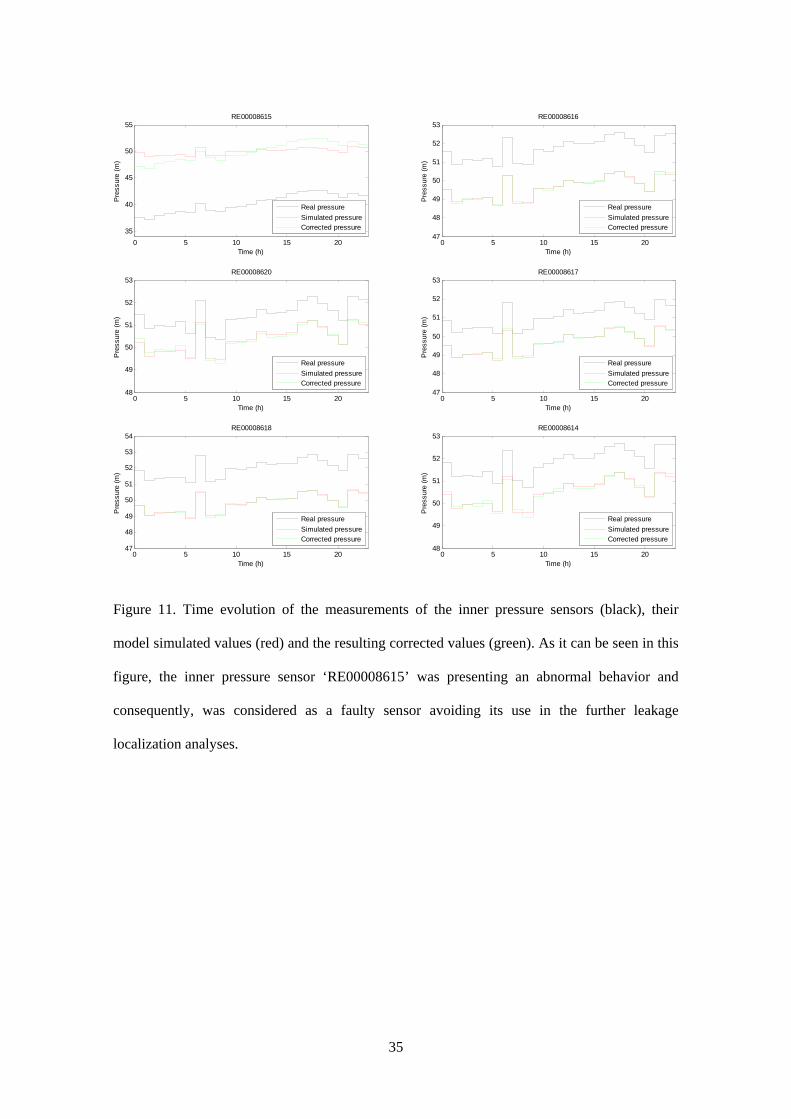
Regarding the DMA inner pressure sensors, divergence between real measurements and
the model simulated values may appear (that is, poor calibration, uncertainty about their depth
regarding the ground level). Indeed, before carrying out the leakage scenario considered in this
article, the inner pressure sensor ‘RE00008615’ was presenting an abnormal behavior and
consequently, was considered as a faulty sensor avoiding its use in this analysis. Thereby,
assuming that in December 19th no major leaks were present, and that the rest of pressure
sensors were not faulty, the differences between real and model simulated pressures have been
adjusted in order to correct the uncertainty associated with the sensor calibration (that is,
offsets) and the depths of the sensors. In Figure 11, the time evolution of the measurements of
the six inner pressure sensors, their model simulated values and their resulting corrected values
have been plotted using the data of December 19th. This figure shows that there is a mismatch
between the sensor real measurements and the prediction given by the model. Thereby,
estimating for every sensor the average value of this mismatch and using this value to correct
the sensor measurements, it can be seen that the corrected measurements accurately describe the
17
model predictions. The correction factor used to adjust the sensor measurements and the model
predictions have been used to update the known but inaccurate sensor depths when the leakage
localization methodology has been applied in the December 20th to determine the localization of
the existing leakage.
Leakage localization methodology application
Applying the data analysis described in previous subsection the occurrence of leakage
in December 20th was detected and the goodness of the calibrated DMA hydraulic model was
stated using sensor measurements of December 19th. The leakage localization methodology was
applied to analyze the sensor data of December 20th in order to obtain the most probable
locations of the detected leak. This methodology has been packed in a model-driven tool in
order to ease its use when applied to a certain scenario. The tool was used for providing an
hourly result on December 20th Nova Icaria leakage scenario.
When applying this procedure for obtaining the result of a certain hour, it must be taken
into account that the used inner pressure sensors have a constrained resolution of 10 cm. This
low resolution together with existing noise in the measurements may be a source of errors in the
computed results. In order to overcome these negative effects derived from the sensor
constrained resolution, two main strategies have been considered: first, the sensor measurement
considered in a certain hour is the result of applying an average filter to the measured values
during the last hour (6 10-minutal measurements) and second, pressure measurements and
model predictions from consecutive hours can be accumulated along a cumulative time window
of a given length allowing to obtain an accumulated observed residual and an accumulated
sensitivity matrix. In the present case, a 10 hour-length cumulative window has been used so the
observed residuals and the sensitivity matrices from the last ten hours are used to generate the
resulting correlation vector at each step which let determines those nodes with the highest
probability to contain the leakage. Thereby, in order to analyze the leakage scenario, data from
18
December 20th to December 21st have been used obtaining one resulting correlation vector at
each time instant (one hour).
The leakage localization methodology output is a correlation vector with as many
components as potential locations of the leakage. Thereby, the value of the jth-component
determines the correlation between the observed residual and the theoretical residual predicted
by the model which would be obtained if the leakage were placed in the jth-node of the network.
So, the correlation vector can be represented graphically on the top of cartography layer of the
DMA using a grey map where the highest correlations are darker than lower ones. The level of
grey depends on the highest correlation obtained at every time instant. This means that the
graphical representation associated with a certain time instant cannot be directly compared with
the one of another time instant since the associated highest correlation value may be different. In
this graphical representation, those nodes with the highest correlation value are depicted with a
black star. Besides, a red cross points the gravity centre of those nodes whose correlation value
is bigger or equal than the 99% of the highest correlation set according to the coordinates of
every node.
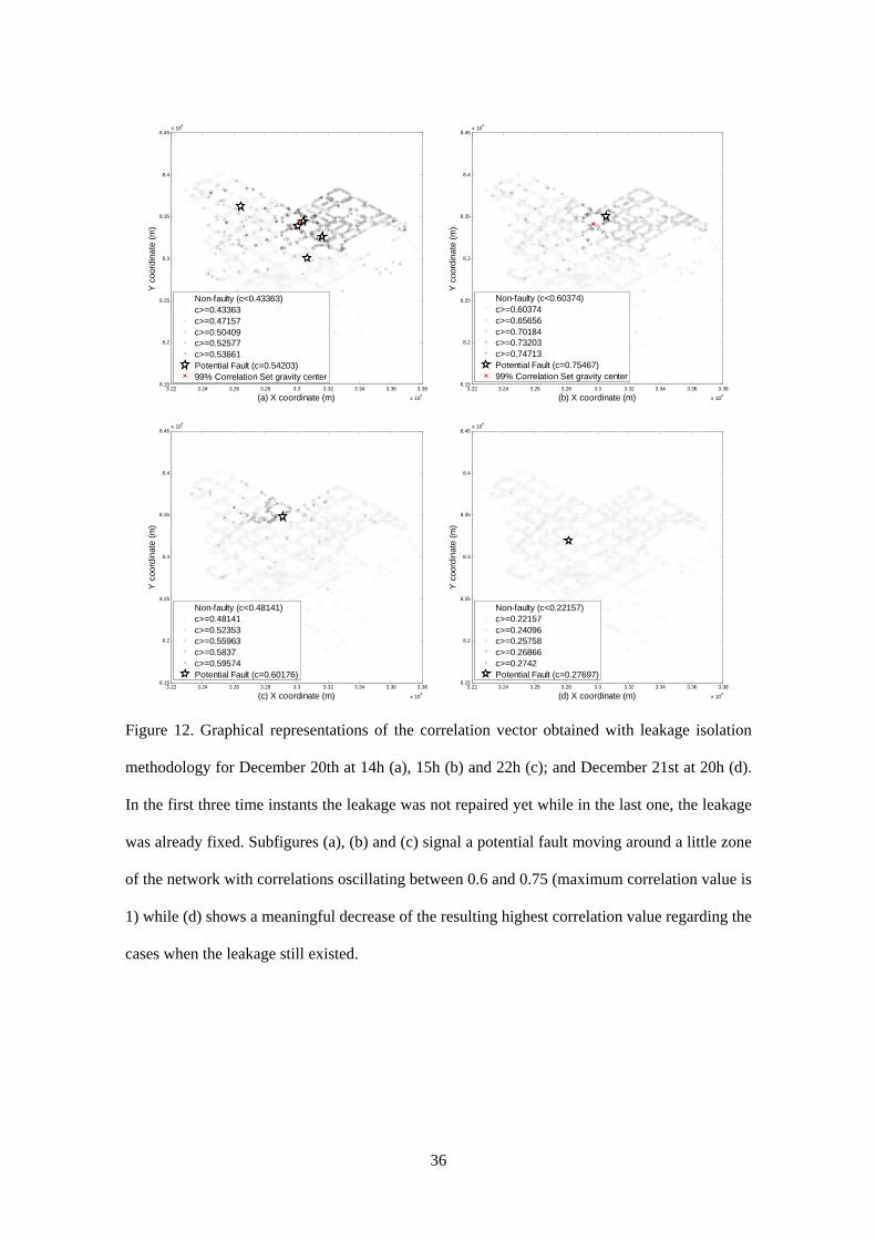
Figure 12 shows four graphical representations of the correlation vector obtained with
leakage isolation methodology for December 20th at 14 h (a), 15 h (b) and 22 h (c); and
December 21st at 20 h (d). In the first three time instants, the leakage was not repaired yet while
in the last one, the leakage was already fixed. Thus, the first three subfigures (a, b and c) signal
a potential leak moving around a little zone of the network with correlations oscillating between
0.6 and 0.75 (maximum correlation value is 1). The last subfigure (d) depicts the correlation
vector once the leakage has been fixed pointing out the meaningful decrease of the resulting
highest correlation value regarding the cases when the leakage still existed.
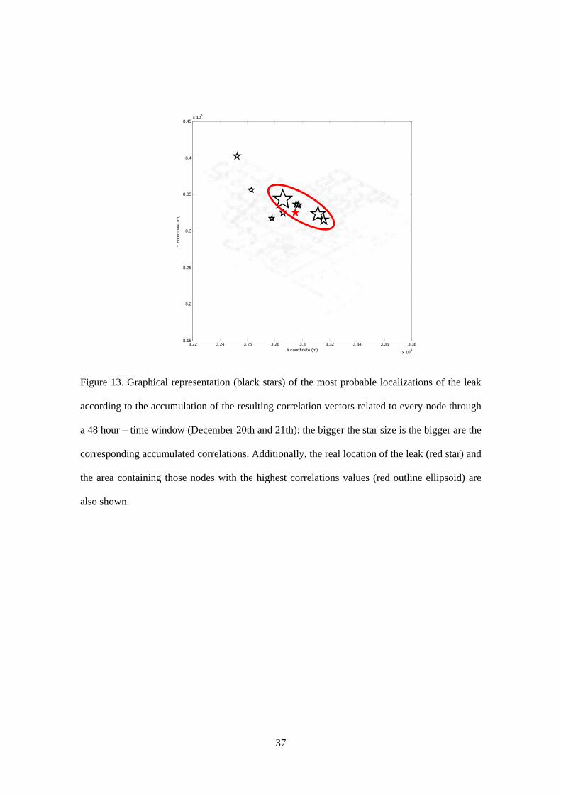
In Figure 13, the resulting correlation vectors obtained at every time instant during
December 20th and 21st have been accumulated in order to determine the nodes with the highest
correlation. Consequently, the most probable localizations of the leak according to this 48 hour
19
– time window are determined (only those correlation values higher than 0.5 are considered). In
this manner, the star size has been plotted according to the resulting value of the accumulated
correlation: the bigger the size is, the bigger are the corresponding accumulated correlations.
Additionally, in this figure the real location of the leak has also been signaled using a red star
and that area containing the nodes with the higher accumulated correlation values has been
marked using an ellipsoid with a red outline. Comparing the leakage localization indications
given by the proposed methodology with the real localization of the leakage, the resulting error
is considered acceptable in the sense that the leak localization predicted area has an acceptable
size containing the real localization of the leak. It must be considered that mainly the resulting
error is due to the errors / uncertainty that may exist in the hydraulic and demand models and in
sensor measurements. Moreover, it is also valuable to consider that a nodal leak localization
using a small set of sensors tends to determine potential network areas where the leak could be
rather than the exact node where the leakage could be. Mainly, this is because when using few
sensors, there could be certain leaks causing the same pressure disturbance from the point of
view of the used sensor and consequently, isolation among them cannot be carried out.
Conclusions
This article has presented a model based methodology for leakage detection and
isolation in water distribution networks (WDN) using pressure measurements. The method is
based on generating residuals between the pressure measurements and their estimation using the
network model that characterizes its behavior without leaks. Those residuals are compared with
the leak sensitivity matrix that contains the effect of each potential node leak in each
measurement. Leak isolation relies on correlating the residuals with the fault sensitivity matrix.
The proposed methodology has been implemented in software tool that interfaces with a GIS
system and allows the easy use by the engineers responsible of the network monitoring.
Simulation results obtained applying the proposed approach to a District Metered Area (DMA)

20
of Barcelona water distribution network have shown the effectiveness and robustness of the
proposed approach. Finally, a real application of the correlation-based method on the pilot tests
has been presented showing satisfactory results in real fault scenarios.
Acknowledgments
This work has been partly funded in by Real-Time Network Monitoring project (ref.
AM0901) of R+i Alliance and by the Spanish MINECO through SHERECS project (ref.
DPI2011-26243).

21
References
[1] A. O. Lambert, “International report: water losses management and techniques”,
Water Science and Technology: Water Supply, vol. 2, no. 4, pp. 1-20, 2002.
[2] A. F. Colombo, P. Lee, and B. W. Karney, “A selective literature review of
transient-based leak detection method”, Journal of Hydro-environment Research, vol. 2, no. 4,
pp. 212-227, 2009.
[3] J. Yang, Y. Wen, and P. Li, “Leak location using blind system identification in
water distribution pipeline”, Journal of Sound and Vibration, vol. 310, pp. 134-148, 2008.
[4] H. V. Fuchs, and R. Riehle, “Ten years of experience with leak detection by acoustic
signal analysis”, Applied Acoustics, vol. 33, pp. 1-19, 1991.
[5] J. M. Muggleton, M. J. Brennan, and R. J. Pinnington, “Wavenumber prediction of
waves in buried pipes for water leak detection”, Journal of Sound and Vibration, vol. 249, no. 5,
pp. 939-954, 2002.
[6] J. Mashford, D. De Silva, D. Marney, and S. Burn, “An approach to leak detection
in pipe networks using analysis of monitored pressure values by support vector machine”, in .
Proc. 3rd International Conference on Network and System Security, Gold Coast, AU, 2009, pp.
534-539.
[7] D. Covas, and H. Ramos, “Hydraulic transients used for leak detection in water
distribution systems”, Proc. 4th International Conference on Water Pipeline Systems, York,
UK, 2001, pp. 227-241.
[8] A. K. Soares, D. Covas, and L. Reis, “Leak detection by inverse transient analysis in
an experimental PVC pipe system”, Journal of Hydroinformatics, vol. 13, no. 2, pp. 153-166,
2011.
22
[9] M. Ferrante, and B. Brunone, “Pipe system diagnosis and leak detection by
unsteady-state tests, 1. Harmonic analysis”, Advances in Water Resources, vol. 26, no. 1, pp.
95-105, 2003.
[10] M. Ferrante, and B. Brunone, “Pipe system diagnosis and leak detection by
unsteady-state tests. 2. Wavelet analysis”, Advances in Water Resources, vol. 26, no. 1, pp. 107-
116, 2003.
[11] R. S. Pudar, and J. A. Ligget, “Leaks in pipe networks”, Journal of Hydraulic
Engineering, vol. 118, no. 7, pp. 1031-1046, 1992.
[12] R. Pérez, V. Puig, J. Pascual, A. Peralta, E. Landeros, and Ll. Jordanas, “Pressure
sensor distribution for leak detection in Barcelona water distribution network”, Water Science &
Technology: Water Supply, vol. 9, no. 6, pp. 715-721, 2009.
[13] R. Pérez, V. Puig, J. Pascual, J. Quevedo, E. Landeros, and A. Peralta,
“Methodology for leakage isolation using pressure sensitivity analysis in water distribution
networks”, Control Engineering Practice, vol. 19, no. 10, pp. 1157-1167, 2011.
[14] J. Ragot, and D. Maquin, “Fault measurement detection in an urban water supply
network”, Journal of Process Control, vol. 16, no. 9, pp. 887-902, 2006.
[15] J. J. Gertler, Fault Detection and Diagnosis in Engineering Systems, Marcel
Dekker, 1998.
[16] M. Blanke, M. Kinnaert, J. Lunze, and M. Staroswiecki, Diagnosis and Fault-
Tolerant Control, 2nd Ed, Springer, 2006.
[17] J. Quevedo, R. Pérez, J. Pascual, V. Puig, G. Cembrano, and A. Peralta,
"Methodology to detect and isolate water losses in water hydraulic networks: application to
Barcelona water network", in Proc 8th IFAC International Symposium on Fault Detection,
23
Supervision and Safety for Technical Processes (SAFEPROCESS), Mexico City, MX, 2012, pp.
922-927.
[18] A. Lambert, “Accounting for losses: the burst and background concept”. Water and
Environment Jounal, vol. 8, no. 2, pp. 205-214, 1994.
[19] M. Farley, and S. Trow. Losses in Water Distribution Networks, IWA Publishing
UK, 2003.
[20] R. Pérez, J. Quevedo, V. Puig, F. Nejjari, M. À. Cuguero, G. Sanz, and J. M.
Mirats, “Leakage isolation in water distribution networks: a comparative study of two
methodologies on a real case study”, Proc 19th Mediterranean Conference on Control &
Automation (MED), Corfu, GR, 2011, pp. 138–143.
[21] J. Quevedo, M. À. Cuguero, R. Pérez, F. Nejjari, V. Puig, and J. M. Mirats,
“Leakage location in water distribution networks based on correlation measurement of pressure
sensors”, Proc. IWA Symposium on System Analysis and Integrated Assessment
(WATERMATEX), San Sebastián, ES, 2011, pp. 290-297.
[22] “ARV 121: Enhancing ADC resolution by oversampling”, ATMEL 8-bit
microcontrollers application note. Available at http://www.atmel.com/images/doc8003.pdf.
[23] R. Pérez, F. Nejjari, V. Puig, J. Quevedo, G. Sanz, M. À. Cugueró, and A. Peralta,
“Study of the isolability of leaks in a network depending on calibration of demands,” Proc. 11th
International Conference on Computing and Control for the Water Industry, Exeter, UK, 2011,
pp. 455-460.
[24] L. A. Rossman, EPANET 2 Users Manual. Water Supply and Water Resources
Division, National Risk Management Research Laboratory, 2000. Available at
http://www.epa.gov/nrmrl/wswrd/dw/epanet.html.

24
[25] J. Meseguer, J. M. Mirats, and G. Cembrano, Puig V., Quevedo J., Pérez R., Sanz
G., Ibarra D. “Web-based software tool (DSS) for on-line leakage localization based on pressure
sensitivity analysis”, submitted to the Journal of Environmental Modelling & Software.
[26] G. Sanz, and R. Pérez, “Demand pattern calibration in water distribution
networks”, Proc. 12th International Conference on Computing and Control for the Water
Industry, Perugia, 2013.
25
Figure 1. Steps of the proposed leak localization methodology. (1) generate residuals from
model with and without leakage (2) generate the signature matrix (3) generate residuals from
model without leakage and measurements (4) generate the signature (5) compare signatures (6)
aggregate and present results.
26
Figure 2. Example of Sensitivity matrix for a simplification of the Icaria Network where 15
nodes have been chosen. Pressure residuals are calculated in the 15 nodes when the leak is in
any of these 15 nodes.
12
3 45
6 78
9 1011
12 1314
15
1 2 3 45 6 7 8 9
101112131415
0
1
2
3
4
5
6
7
Nodos con fuga
Matriz de sensibilidad
Nodos con sensor
Leaky nodesmeasured nodes

27
Figure 3. Results obtained with the correlation method. Maximum correlation (that is 1)
corresponds to the real leak signaled by star and romb. The grey scale represents the correlation
of each node.
3.22 3.24 3.26 3.28 3.3 3.32 3.34 3.36 3.38
x 104
8.15
8.2
8.25
8.3
8.35
8.4
8.45x 10
4
X coordinate [m]
Y c
oord
inat
e [m
]
Fault Isolation, 16 hour data
Error distance: Average = 0m
NodesUnfaulty (c<0.8)
c>=0.8
c>=0.98
c>=0.99
Potential Fault (c=1)Real Fault
28
Figure 4. Leakage analysis results visualization corresponding to an off-line simulation.
29
Figure 5. Conceptual scheme of the DSS for leakage localization.
30
Figure 6. Conceptual scheme of a leakage localization analysis at time instant k.
DMA inlets:Pressure / InflowMeasurements
(k≥time instant>k‐1)
DMA EPANET HydraulicModel
DMA DemandPatterns
Step 1 ‐ DMA hydraulic modelcalibration
(time instant k)
DMA PotentialLeakages
Step 2 ‐ DMA hydraulic model simulation considering potential
DMA leakages(time instant k)
DMA Inner PressureSensor
Measurements(k≥time instant>k‐1)
DMA PressureSensor
Prediction(time instant k)
DMA PressureSensor
Prediction(time instant k)
Free‐Leakage Scenario All Potential Leakages
Step 3 – Computing the fault signal vector Φ
(time instant k)
Step 4 – Computing the theoretical fault signature matrix FSM
(time instant k)
Step 5 – Leakage localization result(time instant k)
LeakageLocalization
(time instant k)
31
Figure 7. Water network of Nova Icaria DMA (EPANET model) highlighting inner pressure
sensors (green stars) and DMA inlets (red stars).
32
Figure 8. Water network of Nova Icaria DMA (EPANET model) highlighting inner pressure
sensors (green stars), DMA inlets (red stars) and the exact location of the forced leak (red
arrow).
33
Figure 9. Leak size estimation. (a) Time evolution of the Nova Icaria DMA total inflow during
the 20th December 2012 affected by the leakage event and during the 19th December 2012
unaffected by the leakage. (b) Time evolution of the difference between these two previous
flows (a) and its average value (leakage size estimation).
0 5 10 15 2020
40
60
80
100
(a) Time (h)
Flo
w (
l/s)
Dec. 19th
Dec. 20th
0 5 10 15 20
0
5
10
15
20
X= 10Y= 5.6077
(b) Time (h)
Flo
w (
l/s)
Flow difference
Leakage mean loss
34
Figure 10. Time evolution of the measured (green) and predicted (blue) inflows in Alaba (a) and
Llull (b) inlets for December 19th showing the degree of accurateness achieved once the
hydraulic model has been calibrated.
2 4 6 8 10 12 14 16 18 20 220
10
20
30
40
50
(a) Time(h)
Flo
w (
l/s)
Real
Predicted
2 4 6 8 10 12 14 16 18 20 220
10
20
30
40
50
(b) Time(h)
Flo
w (
l/s)
Real
Predicted
35
Figure 11. Time evolution of the measurements of the inner pressure sensors (black), their
model simulated values (red) and the resulting corrected values (green). As it can be seen in this
figure, the inner pressure sensor ‘RE00008615’ was presenting an abnormal behavior and
consequently, was considered as a faulty sensor avoiding its use in the further leakage
localization analyses.
0 5 10 15 20
35
40
45
50
55
Time (h)
Pre
ssur
e (m
)RE00008615
Real pressure
Simulated pressureCorrected pressure
0 5 10 15 2047
48
49
50
51
52
53
Time (h)
Pre
ssur
e (m
)
RE00008616
Real pressure
Simulated pressureCorrected pressure
0 5 10 15 2048
49
50
51
52
53
Time (h)
Pre
ssur
e (m
)
RE00008620
Real pressure
Simulated pressureCorrected pressure
0 5 10 15 2047
48
49
50
51
52
53
Time (h)
Pre
ssur
e (m
)
RE00008617
Real pressure
Simulated pressureCorrected pressure
0 5 10 15 2047
48
49
50
51
52
53
54
Time (h)
Pre
ssur
e (m
)
RE00008618
Real pressure
Simulated pressureCorrected pressure
0 5 10 15 2048
49
50
51
52
53
Time (h)
Pre
ssur
e (m
)RE00008614
Real pressure
Simulated pressureCorrected pressure
36
Figure 12. Graphical representations of the correlation vector obtained with leakage isolation
methodology for December 20th at 14h (a), 15h (b) and 22h (c); and December 21st at 20h (d).
In the first three time instants the leakage was not repaired yet while in the last one, the leakage
was already fixed. Subfigures (a), (b) and (c) signal a potential fault moving around a little zone
of the network with correlations oscillating between 0.6 and 0.75 (maximum correlation value is
1) while (d) shows a meaningful decrease of the resulting highest correlation value regarding the
cases when the leakage still existed.
3.22 3.24 3.26 3.28 3.3 3.32 3.34 3.36 3.38
x 104
8.15
8.2
8.25
8.3
8.35
8.4
8.45x 10
4
(a) X coordinate (m)
Y c
oord
inat
e (m
)
Non-faulty (c<0.43363)c>=0.43363c>=0.47157c>=0.50409c>=0.52577c>=0.53661Potential Fault (c=0.54203)99% Correlation Set gravity center
3.22 3.24 3.26 3.28 3.3 3.32 3.34 3.36 3.38
x 104
8.15
8.2
8.25
8.3
8.35
8.4
8.45x 10
4
(b) X coordinate (m)
Y c
oord
inat
e (m
)
Non-faulty (c<0.60374)c>=0.60374c>=0.65656c>=0.70184c>=0.73203c>=0.74713Potential Fault (c=0.75467)99% Correlation Set gravity center
3.22 3.24 3.26 3.28 3.3 3.32 3.34 3.36 3.38
x 104
8.15
8.2
8.25
8.3
8.35
8.4
8.45x 10
4
(c) X coordinate (m)
Y c
oord
inat
e (m
)
Non-faulty (c<0.48141)c>=0.48141c>=0.52353c>=0.55963c>=0.5837c>=0.59574Potential Fault (c=0.60176)
3.22 3.24 3.26 3.28 3.3 3.32 3.34 3.36 3.38
x 104
8.15
8.2
8.25
8.3
8.35
8.4
8.45x 10
4
(d) X coordinate (m)
Y c
oord
inat
e (m
)
Non-faulty (c<0.22157)c>=0.22157c>=0.24096c>=0.25758c>=0.26866c>=0.2742Potential Fault (c=0.27697)
37
Figure 13. Graphical representation (black stars) of the most probable localizations of the leak
according to the accumulation of the resulting correlation vectors related to every node through
a 48 hour – time window (December 20th and 21th): the bigger the star size is the bigger are the
corresponding accumulated correlations. Additionally, the real location of the leak (red star) and
the area containing those nodes with the highest correlations values (red outline ellipsoid) are
also shown.
3.22 3.24 3.26 3.28 3.3 3.32 3.34 3.36 3.38
x 104
8.15
8.2
8.25
8.3
8.35
8.4
8.45x 10
4
X coordinate (m)
Y c
oord
inat
e (m
)
38
AUTHOR INFORMATION
Ramon Pérez received the M.Sc. degree in Physics in 1993 from the University of
Barcelona and the Ph.D. degree in physics in 2003, from the Technical University of Catalonia
(UPC), Terrassa, Spain. He has currently a position as a lecturer at the Department of Automatic
Control at the same university. His current research interests include control and supervision
specially focused in water systems. He joins Advanced Control Systems (SAC) research group
at the Universitat Politècnica de Catalunya and Technological Center of Manresa (CTM).
Gerard Sanz received the M.Sc. degree in Automatic Control and Electronics in 2011
from the Technical University of Catalonia, Terrassa, Spain. He is currently developing his Ph.
D. Thesis in Automatic Control, Robotics and Computer vision. His current research interests
focuses in modeling and supervision applied to water systems.
Vicenç Puig received the Telecommunications Engineering Degree in 1993 and the
PhD Degree in Control Engineering in 1999, both from the Technical University of Catalonia
(UPC), Barcelona, Spain. He is currently Professor of Automatic Control and leader of the
Advanced Control Systems (SAC) research group at the Universitat Politècnica de Catalunya.
His main research interests are fault detection and isolation (FDI) of fault-tolerant control (FTC)
of dynamic systems as well as model predictive control of large-scale systems with special
emphasis on water systems. He has been involved in several European projects and networks
and has published about 200 papers in international conference proceedings and about 45 in
scientific journals.
Joseba Quevedo received the M.Sc. degree in Electrical, Electronic and Control
Engineering in 1973 and the PhD in Control Engineering from the University Paul Sabatier of
Toulouse (France) in 1976 and the PhD in Computer Engineering from the Technical University
of Catalonia in 1982. Since 1979 he is with the Technical University of Catalonia where he is
full professor since 1990. His current research interests include advanced control, identification
and parameter estimation, fault detection and diagnosis, and fault tolerant control and their
applications to large scale systems and to industrial processes.

39
Miquel Àngel Cugueró Escofet received the MSc degree in Control Engineering in
2004 and the PhD degree in Control Systems in 2010, both from the Technical University of
Catalonia (UPC). He currently holds a postdoctoral position in the Intelligent Control Systems
group (SIC) at the same university. His current research activities include model-based fault
diagnosis in water network systems.
Fatiha Nejjari received the M.Sc. degree in physics from Hassan II University,
Casablanca, Morocco, in 1993 and the Ph.D. degree in automatic control from Cadi Ayyad
University, Marrakech, Morocco, in 1997. She is currently an Associate Professor with the
Department of Automatic Control, Universitat Politècnica de Catalunya (UPC). She is also a
Member of the Aeronautical and Space Science Research Centre, UPC. Her active research
areas include nonlinear control, parameter and state estimation, model-based fault diagnosis,
and fault-tolerant control.
Jordi Meseguer received the M.Sc. degree in industrial engineering in 1997 and the
Ph.D. degree in Control Engineering in 2009, both from the Technical University of Catalonia,
UPC. He joined at AGBAR Group in 2001 as IT Analyst. Currently, he is a member of the
Asset Efficient Management research program at CETaqua (AGBAR Group). His current
research interests are focused on model-based fault tolerant-control applied to water systems.
Gabriela Cembrano received her MSc and PhD degrees in Industrial Engineering and
Automatic Control from the Technical University of Catalonia (UPC) in 1984 and 1988
respectively. Since 1989, she is a tenured researcher of the Spanish National Research Council
(CSIC) at IRI. Her main research area is control engineering and she has been involved in
numerous industrial projects on modeling and optimal control of water supply, distribution and
urban drainage system since 1985. She has taken part in several Spanish and European research
projects in the field of advanced control and especially its application in water systems.
Currently, she the leader of WATMAN project on modeling and control of systems in the water
cycle, funded by the Spanish Ministry of Science and Innovation (2010-12) and Scientific
Director of EC project EFFINET Integrated Real-time Monitoring and Control of Drinking
40
Water Networks FP7 ICT-318556 (2012-14). She has published and co-authored over 50
journal and conference papers in this field.
Josep M. Mirats Tur, M.Sc. in Telecommunication Engineering (Technical University
of Catalonia, UPC) and Ph.D. at the Institute of Robotics of Barcelona in 2001. He has been a
research visitor at the UT (USA), the UNINA (Italy), and an invited professor at the ITESM in
Mexico. He has been a visiting scholar at U. Cambridge (UK) and the UCSD (USA) to study
tensegrity structures. He has co-authored more than 40 publications and participated in more
than 20 collaborative projects. He leads CETAQUA’s participation in the EFFINET project on
real-time network monitoring.
Ramon Sarrate received the M.Sc. and Ph.D. degrees in industrial engineering from
the Universitat Politècnica de Catalunya, Terrassa, Spain, in 1994 and 2002, respectively. He is
currently a Collaborating Professor with the Department of Automatic Control, Universitat
Politècnica de Catalunya. His current research interests include model-based fault diagnosis and
hybrid systems.