Embed Size (px)
Citation preview

LUND UNIVERSITY
PO Box 117221 00 Lund+46 46-222 00 00
Leaching of concrete : experiments and modelling
Ekström, Tomas
2001
Link to publication
Citation for published version (APA):Ekström, T. (2001). Leaching of concrete : experiments and modelling. Division of Building Materials, LTH, LundUniversity.
Total number of authors:1
General rightsUnless other specific re-use rights are stated the following general rights apply:Copyright and moral rights for the publications made accessible in the public portal are retained by the authorsand/or other copyright owners and it is a condition of accessing publications that users recognise and abide by thelegal requirements associated with these rights. • Users may download and print one copy of any publication from the public portal for the purpose of private studyor research. • You may not further distribute the material or use it for any profit-making activity or commercial gain • You may freely distribute the URL identifying the publication in the public portal
Read more about Creative commons licenses: https://creativecommons.org/licenses/Take down policyIf you believe that this document breaches copyright please contact us providing details, and we will removeaccess to the work immediately and investigate your claim.

LUND INSTITUTE OF TECHNOLOGY
Division of Building Materials
LEACHING OF CONCRETE
Experiments and Modelling
Tomas Ekström
Report TVBM-3090 2001

I
PREFACE This work has been carried out at the Division of Building Materials at the Lund Institute of
Technology and has been financed by Swedish National Board for Industrial and Technical Development (NUTEK), Elforsk AB and Sydkraft AB, Miljö och Utveckling. The research project was initiated by NUTEK and professor Kyösti Tuutti, Skanska Teknik.
My supervisor has been Göran Fagerlund, whom I wish to thank for his support and inspiration.
I would also to thank my colleagues at the Div.of Building Materials for their help and support. A special thanks to Björn Johannesson for discussion about mode1ling, Mårten Janz for helping me with the experimental determination of the water retention curves, Sture Lindmark for a decisive idea concerning the water pressure equipment, Stefan Backe for his quick and effective he1p with cornputers and finally Bo Johansson and Ingemar Larsson for he1p in the laboratory.
I would also express my gratitude to my company Sycon Energikonsult AB with staff for having such patience with my studies.
The work presented in this report is almost identical with the licentiate thesis report TVBM-7153 (Ekström 2000), but the results have been further developed and analys ed.

II
Contents
PREFACE
ABSTRACT
SUMMARY
LIST OF SYMBOLS AND ABBREVIATIONS
1. INTRODUCTION 1.1 General about leaching and its effects 1.2 literature survey
1.2.1 Introduction 1.2.2 The leaching process 1.2.3 Factors influencing leaching 1.2.4 Leaching effect on penneability 1.2.5 Leaching effect on porosity 1.2.6 Leaching effect on strength 1.2.7 Synergy between leaching and other environmental attacks 1.2.8 Conc1uding remarks
1.3 Research needs 1.4 Short description of the present study
2. LEACHING PROCESS 2.1 General 2.2 Chemical influences on the process
2.2.1 Chemical structure of concrete 2.2.2 Dissolving reactions 2.2.3 Mobility of ions in concrete
2.3 Physical influences on the process 2.3.1 Physical structure of concrete 2.3.2 Mobility of water in concrete
3. LEACHING MODELS USED IN THIS WORK 3.1 Introduction 3.2 The leaching process 3.3 Strength models for concrete 3.4 Degradation model 3.5 Dissolving reaction
4. SCOPE AND GENERAL LAYOUT OF THE EXPERIMENTAL WORK
5. THE EXPERIMENTAL PROCEDURES 5.1 Test equipment
5.1.1 Test water 5.1.2 Pressure equipment 5.1.3 Test cells 5.1.4 Oudet
I
v
VI
IX
1 1 5 5 5
16 22 25 25 27 27 27 28
29 29 35 35 39 44 45 45 48
55 55 56 60 64 65
68
73 73 73 73 74 74

m
5.2 Test procedure 74 5.2.1 Mounting in test cells and measurements of water flow 74 5.2.2 Permeability analysis 75 5.2.3 Chemical analysis in collected water samples 75 5.2.4 Chemical analysis of concrete 77 5.2.5 Porosity analysis 78 5.2.6 Analysis of mechanical properties 80 5.2.7 Dissolving rate of Ca(OH)2 in de-ionised water 80
5.3 Validity of the tests 81 5.4 Reliability of the tests 85
5.4.1 Introduction 85 5.4.2 Permeability analysis 85 5.4.3 Chemical analysis of drainage water 91 5.4.4 Chemical analysis in concrete 93 5.4.5 Porosity analysis 93 5.4.6 Mechanical properties 93
6. CONCRETE 94 6.1 Introduction 94 6.2 Cement 94 6.3 Admixtures and additives 94 6.4 Aggregate 94 6.5 Mixing and curing water 96 6.6 Recipes 96 6.7 Casting 96 6.8 Curing 96
7. RESULTS OF EXPERIMENTAL WORKS 98 7.1 Permeability 98 7.2 Chemical analysis of the drainage water 104
7.2.1 General 104 7.2.2 Leaching of Ca 105 7.2.3 Leaching of K and Na 106 7.2.4 Leaching of S 106 7.2.5 Leaching of Mg, Fe and Si 106 7.2.6 Changes in pH 106 7.2.7 Summary 106
7.3 Chemical analyses of the water at the upstream face 107 7.4 Chemical analysis of the leached concrete 109 7.5 Porosity 111
7.5.1 Total porosity 111 7.5.2 Pore size distribution 113
7.6 Mechanical properties 113 7.6.1 Compressive strength 113 7.6.2 Elastic modulus 115
7.7 Dissolving rate of Ca(OH)2 in de-ionised water 115
8. DISCUSSION OF RESULTS AND MODELLING OF THE LEACHING PROCESS 117 8.1 Introduction 117 8.2 Discussion of permeability results 117

8.3 Leaching of substances 8.3.1 Introduction
IV
8.3.2 Leaching of ions to water at the upstream face 8.3.3 Leached ions in the drainage water 8.3.4 Unleached components in the specimen
8.4 Porosity 8.5 Mechanical properties
8.5.1 Compressive strength 8.5.2 Elastic modulus
8.6 Leaching modell versus the experimental results 8.7 Dissolution of Ca(OHh in pure water 8.8 Conc1usions
8.8.1 Experiments 8.8.2 Modelling 8.8.3 Future research
REFERENCES
Test cells. Evaporation from measuring vessels. Sieve curves of aggregate. Overview of casting, curing and leaching tests. Experiment 2: water flow and permeability. Experiment 3: water flow and permeability. Permeability. Mean values and standard deviation.
121 121 121 126 131 133 135 135 136 136 142 143 143 144 145
146
Appendix 5-1 Appendix 5-2 Appendix 6-1 Appendix 6-2 Appendix 7-1 Appendix 7-2 Appendix 7-3 Appendix 7-4 Appendix 7-5
Experiment 2: water flow and content of calcium in drainage water. Experiment 2: water flow and content of potassium and sodium in drainage water.
Appendix 7-6 Appendix 7-7
Appendix 7-8 Appendix 8-1
Experiment 2: Content of sulphate in drainage water. Experiment 2: summary of the content of studied elements Ca, K, Na, S and pH in drainage water. Experiment 2: stress-strain curves of drilled-out cores. Leaching rate of calcium and potassium.

v
ABSTRACT The report contains a literature survey of concrete leaching, and presents the results of an experimental determination of leaching. Deionized water was pressed through a number of defect-free concrete specimens in order to study lime leaching. The result showed low and uniform water flow during the first time. After a certain period, however, most specimens obtained a rapidly increased flow. This was probably due to breakthrough in some distinct percolation paths. Around these paths of "flow pipes" the solid material was leached and the concrete became disintegrated with almost no continuos cementitious materialleft to maintain strength and tightness. The main results of the experimental study are presented. A model for how to model the leaching process and its effects, is theoretically outlined and applied to the experimental data.
Key words: concrete dams, leaching, water permeability.

VI
SUMMARY Many concrete dams, and other concrete structures within the hydropower industry in Sweden
and other western countries, are old and in a more or less severe state of degradation. The economical value of these structures is very high. Besides, they are urgently needed for production of electricity. Leaching is, together with freeze-thaw, the most common degradation problem in Swedish hydraulic concrete structures. In mountainous terrain, river water is often relatively free from dissolved ions (soft water). Such water is aggressive to concrete structures because of its high dissolving ability. In leaching of concrete, hydration products are dissolved from the pore system of the concrete and transported away by ion diffusion or by the water flow. When solid material is leached, porosity and permeability will increase and strength will decrease. Influencing factors that increase leaching are; (i) high permeability of the concrete and any increase of permeability due to leaching, (ii) high amount of calcium in the concrete, especially calcium hydroxide, (iii) high content of carbon dioxide in the water (iv) low hardness of the water (soft water).
Published literature before 1970 mainly deals with percolation of concrete, i.e. concrete exposed to water pressure with resulting water and ionic flow through the concrete. Also extraction studies of concrete i.e. concrete that lays in stagnant aggressive water with a resulting diffusion of ions to the water, are reported.
literature after 1970 deals also with extraction studies with careful analysis and modelling of the ionic diffusion from cement paste or mortar to the outside water. Self-healing phenomena where the permeability decreases are also treated both in cracks and in homogenous concrete.
A leaching process starts when water dissolves compounds in pore walls inside the concrete. A dis solution can be looked upon as a diffusion process where, (i) water molecules diffuses to the reaction place in the pore walls, (ii) water molecules dissolve solid compounds, (iii) the dissolved compounds are transported away from the reaction place to the pore solution. The dis solution rate of different compounds in concrete depends on the solubility of the actual compound and on how elose the compound is to pure water. Except for potassium hydroxide and sodium hydroxide, which are always in the pore solution, calcium hydroxide is the most soluble compound in concrete. Calcium silicate hydrates and aluminium ferrite phases are less soluble, but the more calcium that is incorporated in these phases, the more soluble they are. When the pore walls become poor of soluble compounds, dis solution to the pore solution will decrease and the concentration of dissolved ions in the drainage water, flowing through the structure, will decrease.
The purpose with the experimental work and the modelling was to investigate the flow of deionised water through homogenous concrete and the leaching process. Changes in permeability, leaching rate and strength were therefore studied.
In the leaching model, water is assumed to flow through a number of tortuous flow pipes of different average diameter, within a saturated continuous concrete body. The water flow is calculated by a reduced Hagen-Poiseuilles law, regarding the deviation between flow in a real tortuous flow pipe and flow in a perfect cylinder. In the model, solid material is supposed to be dissolved from the pipe walls and transported downstream, and out of the body. No diffusion of ions in upstream direction is regarded. When solid material is leached, the pipe becomes wider and the water permeability increases. Due to a gradually reduced amount of dissolvable material in the pipe walls, the dissolving rate decreases. Another effect is that the porosity increases and the strength decreases. The concrete body is divided into one element, so any effect of gradients

VIT
of leaching effects throughout the body is not regarded. The model does not consider any selfhealing effect, e.g. re-crystallisation of CaC03• Strength changes is modelled by involving an assumed fictitious strength of the solid phase of the cement paste together with calculated porosity changes due to leaching. The leaching model gives interesting results despite its simplicity and the many assumptions made. The leaching model can easily be connected to ordinary static calculations for estimations of the safety margin for concrete structures over time.
To imitate a concrete dam subjected to soft water under pressure, de-ionised water was pressed through a number of concrete specimens. The experiment was accelerated regarding (i) the pressure gradient, (ii) the water to cement ratio and (iii) the water aggressiveness. The test equipment consisted of a de-ionising aggregate, a storage tank for the de-ionised water, a pump, a pressure tank and a steel pipe system that carried the water to a number of stainless steel test cells in which cylindrical "pressure" specimens of concrete were placed. "Reference" specimens of the same size were cast, hardened and cured in the same way as the pressure specimens were. All specimens were made of ordinary Portland cement of type CEM I 42.5, without any admixtures or additives. Aggregate was of quartzite and had a maximum size of 16 mm. The specimens were made with three different w/c ratios, wie 0.6, 0.8 and 1.3. The specimens were cured in three different ways; (i) virgin specimens were water cured for 2 months, (ii) late-dried specimens were driedone week in oven +55°C after 6 months ofwater curing, (iii) early-heated specimens were wrapped in plastic bags and then heated immediately in an oven in a cycle from +20° to +55-60°C and then down again to +20°C during a week. They were then placed in laboratory air at +20°C for 2 months.
The wie ratios 0.8 and 1.3 were used for virgin and late-dried specimens and the w/c ratios 0.6 and 0.8 for early-heated specimens. All specimens had a height of 50 mm. The diameters was 155 mm and 45 mm. The pressure specimens were cast in conical steel cylinders in which they were later placed during the leaching test. The conical shape, together with silicon grease and a latex tube around the circumference, made the joint between the specimen and the steel cylinder tight. Percolated water, drainage water, was collected in measuring glas ses and measured by volume. Flow of dissolved ions in the drainage water was measured by ion selective electrodes and to some extent by ICP-AES technique (Inductive Coupled Plasma Atom Emission Spectroscopy). Unleached components in one, leached specimens was measured by dissolving the specimen in HN03 and then analysing the solution by ICP-AES. Compressive strength of some leached specimens and of some reference specimens was measured by a strength test machine.
The experimental results shows that pure water percolating the concrete specimens has an ability to dissolve hydration products, probably mainly Ca(OH)2, and also to carry the dissolved ions out of the specimen by diffusion and convection. Depending on the wie ratio and the curing history, the extent of leaching was different. A high water to cemetn ratio made the specimens more porous, resulting in higher water permeability. Virgin specimens had a low and constant permeability with small deviations between the specimens. However, one specimens with w/c 0.8 and one with w/c 1.3 had a rapidly increased permeability after a certain period. Late-dried specimens became 100 times more permeable than in the virgin state. This was probably caused by micro-cracks appearing during drying. Because of the high hydration ratio almost all cement was hydrated and there was not much cement left for any self-healing. The permeability of these specimens often increased rapidly, after some time. Early-heated specimens, had about 100 times higher initial water permeability than the virgin specimens. However, immediately after the test started, the permeability began to decrease in the specimens. After about eight month it

vm
was c10se to the penneability at the virgin state. The reduced penneability was probably caused by re-started hydration and resulting se1f-healing. If the test time had been long enough, probably all specimens had sooner or later been so leached that the penneability had increased once again.
Observations of the specimens indicated that water had flown in a rather few, distinct flow pipes. Also other authors have suggested that the main water flow through concrete, exposed to water pressure, occurs in certain main flow channels, orf/ow pipes, that are continuous throughout the concrete. Such main flow paths can be large-sized capillaries, inter-facial contact zones between paste and aggregate, cracks or construction joints in real structures.
In the tested concrete, water dissolved solids from the walls of such flow pipes and when the pipes grew wider, the water flow increased further and even more solid material was leached. Finally, the pipe walls became so exhausted in lime that the lime leaching rate and the water flow increased only slowly. The dissolution of the pipe walls was govemed by a diffusion process from the interior of the solid towards the pipe wall. Around these pipes the concrete became very disintegrated with almost no continuos cementitious materialleft to maintain strength and tightness. Between the flow pipes, or in less penneable concrete, more of the leaching seems to have been govemed by diffusion to the inlet water at the upstream face of the specimens. A detailed analysis of the residual elements of one specimen also showed that the most important element in concrete, calcium, mostly was leached from the upstream part of the specimen. This was probably due to diffusion in the upstream direction. Another possibility is that penneating water became saturated with lime already at the upstream part due to dissolution of lime. Therefore, its dissolving ability was very much reduced when it reached the deeper parts of the specimen.
Another part of the specimen, which lost quite a lot of calcium, was where the aggregate content was high. The cause of the leaching in this part was probably water percolation in porous and easily soluble areas between the aggregate and the cement paste. Because of leaching, porosity was increased in these parts of the specimen.
The measwed residual content of substances in the leached specimens corresponded fairly well to the measured ionic flow in the drainage water flow. The results also show that when solid material is leached, the porosity will increase. The strength reduction, was to a high degree a local phenomenon. In parts of the specimen, where much solid material had been leached, the strength was very much reduced. But if these parts were small compared to the whole specimen, the average strength of the whole specimen was not much influenced. The number of specimens used for strength testing were however too few for any more detailed analysis of relations between leaching and strength.
The work shows that there is need of more research of leaching. Examples of research areas are; (i) a more precise study of the diffusion of ions upstreams combined with measurements of ions in the drainage water, (ii) experiments of leaching in cracks or other defects and inhomogenities, (iii) studies of porosity changes due to leaching, (iv) studies of strength changes in leached concrete.

IX
List of symbols and abbreviations
All symbols are explained where they first appear in the text. Most of the symbols are also presented here. All dimensions are in SI units
Symbol DeC"mition SIuDit a Approximation matrix of a state variable in the Finite
Element Method (-) A Area (m2)
A Aggregate content (kg) A; Area of pipes with size i at time t (m2)
Asolid lon releasing area in flow pipe walls (m2)
A tot Total area (m2)
B Permeability coefficient (s) c lonic concentration (mole/m\ (moleIl),
(kg/l), (g/l) Ci lonic concentration for specie i (mole/m3)
c;(s) lonic concentration for specie i in a solid phase (mole/m3)
Csat Saturation concentration (mole/m3)
C Cement content (kg) dm; Mass of leached material for pipes with size i (kg) D Constitutive matrix (-) D Diffusion coefficient (m2/s) Da Apparent diffusion coefficient , regarding tortuosity,
constrictivity and chemical reactions with the pore wa11s. (m%)
Df Free water diffusion coefficient (m2/s) dt Time increments (s) E Electrical potential (V) E Energy (J) E Modulus of e1asticity (pa) F Faraday constant (9.65·10~ J/(V ·mole) F i Total ionic flux (mole/(m2·s)) Fiu lonic flux due to diffusion (mole/(m2·s)) F iv lonic flux due to convection (mol/(m2·s)) Jo Fictitious strength of the solid phase without pores (pa) Jo' Fictitious strength of the cement gel with gel pores inc1uded (pa) J;,c Compressive strength of cement paste (pa) g Acceleration of gravity (m/s2)
g(fcck) Model of compressive strength for concrete (pa) I lon strength (moleIl) K Empirical parameter instrength model (-) K Resistance matrix in the Finite Element Method (-)
KR Henry' s constant (molell·atm) Ksp Solubility product (-) kw Water permeability (m/s) k~(t) Water permeability for pipes with size i at time t (m/s) k;on lon diffusivity coefficient (m%) k;on(s) Diffusion coefficient in solid diffusion layers (d/s)

kion(aq)
L L m M lnpaste
Tnwet,air
mwet,water
m,dry,air
Mflushed
N ni p p Pw p p
Pe
Pp
(Peap)p
(Peap)pL
Q Qpipe
Q Q qion
qiondiff
qioneonv
qw qwO q~(t) rh
RH
s So share t tes)
t(aq)
T
V;iPe,leached
x
Diffusion coefficient in pipe solutions Length of flow pipes Length of strength tested cylinders Molarity Molar weight Weight of cement paste Weight of saturated slices in air Weight of saturated slices beneath water Weight of dried (+105°C) slices in air Flushed-out mass of ions from the inlet of the test cells Number of different pipe sizes in a body Number of flow pipes with size i Pressure Partial pressure Water pressure head Wet perimeter Porosity Total porosity of concrete Total porosity of cement paste Capillary porosity in paste before leaching Capillary porosity of paste after leaching source term Source term for one dimensional flow pipe Heat energy Reaction matrix Flow ofions lonic diffusion Convection flow of ions Flow ofwater Initial flow of water Total water flow for pipes with pipe size i at time t Hydraulic radius Relative humidity Circular pore radius Gas constant
(m2/s) (m) (m) (mole/m3) (moleIl) (kg/mole) (kg) (kg) (kg) (kg) (g) (nos.) (nos.) (pa) (atm) (m) (m) (m3/m3)
(m3/m3)
(m3/m3)
(m3/m3)
(m3/m3)
(mole/s) (kg/s) (mole/(ms) (J) (-) (mole/(s)) (mole/s) (mole/s) (m%) (kg/s) (m3/s)
(m3/s) (m) (%) (m) (J/(K·mole) )
Reaction quotient ( -) Reduction coefficient due to deviation between flow in a real tortuous flow pipe and a perfect cylinder ( -) Solubility (kg/m3)
Solubility at time zero (kg/m3)
Share of total pore volume that can percolate water (-) Diffusion layer thickness (m) Thickness of diffusion layers in solids (m) Thickness of diffusion layers in solutions (m) Temperature (K) Volume of leached material for all pipe sizes (m3)
L V~iPe (to) Total pipe volume for pipe size i at time zero
V:ne pipe Volume of one pipe with pipe size i at time zero

Vi p/m
V;ipe,leached
Vp/m
Vgel (VO)a (VO)p Vp
(Vp)a (Veap)p (Vp)gel (Vp)p Va Vair
Ve Vflushed
w W
Wn
W W W/C
X
a dPw
t1t 10
I/J I/Jb
I/J: y <p
Il fl
J.li fliO
V
v
p p Pa pe PM Pw
XI
Total pore volume per kg paste for pipe size i at time zero
Volume of leached material during a time step t1t
Total volume of cement paste per kg paste Volume of cement gel Compact volume of aggregate Compact volume of cement paste Volume of cement paste Pore volume of aggregate Volume of capillary pores in cement paste Volume of gel pores in cement paste Total pore volume of cement paste Volume of aggregate Volume of air due to compaction or air additives Volume of concrete Flushed-out volume of ions from the inlet of the test cells Velocity of water Crack width Work Chemical bonded water Free (or unbound) water fraction Mixing water content Water to cement ratio Gel space ratio Valence of the ionic specie i Degree of hydration Water pressure differences Time step Dielectric constant Diameter Diameter of pipes with size i at time zero
Diameter of pipes with size i at time t
Activity coefficient contact angle between the liquid and the solid tube walls Mean value Dynamic viscosity Electrochemical potential of specie i Standard chemical potential of specie i Coefficient of variation
Nabla operator ( VT = [:x :y :J) Electrical charge density Bulk density Density of the aggregate Density of cement Density of leached material Density of water
(m3Ikg)
(m3)
(m3Ikg) (m3)
(m3)
(m3)
(m3)
(m3)
(m3)
(m3)
(m3)
(m3)
(m3)
(m3)
(litre) (m/s) (m) (J) (kg) (m3/m3)
(kg) (kglkg) (m3/m3)
(-)
(-) (m) (s)
CF/m=J/(V2·m)) (m)
(m)
(m)
(l/mole) (rad) (-) (Ns/m2)
(J/mole) (J/mole) (-)
(J/(V·m3))
(kg/m3)
(kg/m3)
(kg/m3)
(kg/m3)
(kg/m3)

XII
Surface tension between liquid and air Compressive stress Standard deviation Reduction tensor regarding the tortuosity of a pore system
(N/m) (pa) (-) (-)

1 INTRODUCTION
1.1 General abont leaching and its effects
Background
l
Many concrete dams, or other concrete structures in the hydropower industry in Sweden and other western countries, are old and in a state of degradation. These structures are very valuable because they represent a large amount of money invested and they are needed for production of electricity.
Leaching is, together with freeze-thaw, the most common degradation problem in Swedish concrete dams. In northem Sweden, river water is often relatively free from dissolved ions (soft water). Such water is aggressive to concrete structures because of the dissolving ability. It is mostly older dams, with of ten very porous concrete with high water permeability that has leaching problems. But even though they are erected by better methods and made ofbetter concrete, also more recently built dams may be subjected to leaching damages in a near future. So, the knowledge how to predict leaching damages is needed now and even more in the future. This work is about lime leaching in concrete specimens subjected to soft water.
Concrete structures
To be a little witt y one might say that there are two types of rocks; natural rocks (sedimentary, magmatic, and metamorphic) and man-made rocks as concrete structures. Concrete is made of approximate1y the same material as the natural rocks. However, because we do not have the supply of pressure or heat as the other rocks had when formed, the concrete rocks must be made in a chemical way. Cement is used to create cement paste that fix incorporated aggregates in a rigid structure. Cement reacts strongly with mixing water and forms hydration products. During the continuous hydration that can last for long time, a supply of water is needed. If there is no water available, hydration will cease.
Concrete structures are built with the shape and geometry needed to resist loads and to meet other requirements.
Leaching
If concrete is used for a dam in a river, water will penetrate the concrete due to the water pressure and due to the porosity of the concrete. Now, water is not only good for the continuous hydration. On the contrary, water can start to dissolve hydration products in the concrete. Concrete dams are subjected to exactly the same environmental impacts as the naturally built rocks; water will dissolve substances, water will together with low or high temperatures break up parts of the concrete and wind will erode the surfaces. When material dissolves from the rocks, wind and water will carry away the loose parts and the rock will become smaller and weaker.
If percolating water is soft, the leaching effect on the concrete will be strong. The water diffuses inta the concrete and dissolve hydration products (and aggregate if it is easy soluble). Dissolved material will diffuse out of the concrete to the bulk of pure water in the reservoir. This is a slow leaching process.
If water also percolates through the concrete due to pressure gradients, the water will reach much more intemal area of soluble products. Now, dissolved material will also be carried away by the flow of water downstream and out of the concrete. This can be a rapid leaching process, depending on how fast the water is percolated through the concrete and how much intemal area the water will meet on its way.

2
Leaching is the name of the whole process of dissolving and transporting substances out of the concrete.
Leaching effects
When solid material is leached, the porosity will increase and the amount of OH" -ions will decrease in the pore solution and in the pore walls. When the porosity increases, the water penneability will increase and the leaching process will accelerate. When the porosity increases, the strength will also decrease. When the permeability in different parts of a concrete dam changes, interna! pore pressure will also change in the same way. The decreasing strength but also a changed pore pressure may lower the stability for parts of or for the whole dam.
Figure 1-1 shows a old stone-faced concrete dam subjected to lime leaching. Water has percolated the dam and transported dissolved lime to the downstream face of the dam, where the lime have react with atmospheric carbondioxide and formed curtains of calcite. The calcite curtains has probably slowed down the water flow and the lime leaching due to a tightening effect, but the curtains can also change the intemal pore pressure so the pushing force of water become worse.
There are also synergy effects between leaching and other degradation mechanisms. An example is showed in Figure 1-2, where a changed pore structure has changed (decreased) the resistance to freeze-thaw. The figure shows a concrete block supporting a steel tube, which conveys water down to a hydropower station. Rainwater has penetrated from the top of the block and through this. Water has penetrated especially through the slit between the concrete and the tube. The block lay in a slope in the terrain, so the water flows inside the block while dissolving lime and finally both water and the dissolved lime flows out through the downstream face. When coming out from the surface, the leached Ca(OH)2 reacts with CO2 in the air and a hard calcite-Iayer is formed. This layer has increased the water content in this part of the block. This increased water content, together with a possibly coarsened pore system, has in this case lead to substantially freezing damages. These damages open up the concrete for even more flow of water and this circle is running towards a total destruction of the load-bearing capacity of the block.

WateJi."
~ Environment
wads ~
WateJr
3
Poorer mecbanica1 properties Jncreased wafer fiow
Incteased intemal pore pressure SyneIgie with freezo.thawing
Figure 1-1 An old stone-faced concrete dam subjected to lime leaching. Pure water penetrates the cement paste inside the dam or under the dam and dissolve lime and other soluble substances. The white curtains on the downstream face is calcium carbonate formed by atmospheric CO2 and Ca(OH)2 transported by water coming out of the dam.

4
Figure 1-2 Synergy effects between lime leaching and freeze-thaw in a fix-block of concrete, supporting a water tube.
Another synergy effect could be between leaching and reinforcement corrosion. The pH value inside the concrete may decrease due to leaching, and this can fmally open up for reinforcement corrosion.
Structures for which leaching is a problem Most modern concrete structures can withstand leaching very weil. For old dams, badly
designed dams, badly cast dams, badly cured dams, dams in rivers with very pure or acid water and for joints or gate abutments in dams, leaching can be a problem. In the worst case, the leaching may in such structures decrease the strength, increase the intemal forces, decrease the resistance against freeze-thaw and decrease the protection against corrosion on the reinforcement.

1.2 Literature survey
1.2.1 Introduction
5
Halvorsen (1966) performed a large study of lime leaching on water retaining concrete structures. The study is still rather up to date, in part because lime leaching in such structures have not been studied so much the last 30 years. The study also contains a large literature survey. Halvorsen divides leaching into three types: 1) Leaching through very porous concrete. 2) Leaching from free concrete surfaces. 3) Leaching through cracks in concrete.
Due to Halvorsen, leaching studies have only been performed on homogenous, very porous concrete (with percolation and extraction tests) and at concrete surfaces (with extraction tests). By percolatian is meant flows of water that trickle through a homogenous body. An extractian test is to place a homogenous body in stagnant, aggressive water and letting the water dissolve material from the surfaces of the body.
Until1966, not a single leaching test was carried out for cracked concrete! On the other hand, Halvorsen claims that the literature does not show any case where the concrete has been destroyed due to leaching in cracks.
Studies af ter 1966 regards mostly extraction tests with leaching from mortar or cement paste specimens in pure water without pressure gradients. Some percolation tests have been performed with homogenous or cracked concrete subjected to water pressure, but only self-healing effects have been regarded. By self-healing means that the main flow-paths in the concrete are filled with material during time, for example with calcium carbonates coming from re actions between Ca2+ in the pore solution and atmospheric CO2 coming in from surroundings.
Be1ow, some literature regarding the leaching process, influencing parameters on leaching and leaching effects on permeability, porosity and strength is given.
1.2.2 The leaching process
The leaching process is when solid compounds in the concrete are dissolved by water and then transported away, either due to concentration gradients (diffusion) or by the flow of water (convection). External or capillary pressures may for example cause water to flow. For future estimations of leaching degradation in concrete, it is important to have a knowledge about the kinetics and influencing variables on the process, i.e. from the dis solution of solids to the diffusion and the convection of dissolved ions.
Unsworth, Lata and Hubbard (unknown) exposed OPC mortar specimens with de-ionised water under a pressure of 2 Mpa, see Figure 1-3. The results shows a rapid rise of N a in the drainage water up to a maximum content of about 280 (/lg/l) when a water volume corresponding to two pore volumes (PV) had percolated the specimens. The rise of K was almost as rapid as for Na and rise to about 1200 (/lgll), when three PV of water had percolated. At the same time, the pH value rise rapidly up to about 13.1 because of the rise in Na and K. After the maximum values was reached for N a and K, the concentration of these components rapidly decreased again down to very low values at about eight PV. As the content of Na and K started to decline, the pH value declined to about 12.5 and the content of Ca started to rise. After ab out ten PV had been flowed, the content of Ca reached its maximum value of about 530 (/lg/l) and then only slowly (in a logarithmic time scale) decreased to about 460 (J1g/l) after about 80 PV when the test stops. The pH value also decreased slowly as the content of Ca decreased. The

6
water permeability followed a slowly decreasing curve from about 7.10-12 down to 6.10-12 (mls). The result shows that N a and K was quickly washed out of the pore system, followed by a dissolving of Ca to the pore solution. Because of the much larger amount of Ca, than N a and K in the mortar, the leaching rate of Ca was rather constantly high for the whole studied time. However, as Moskvin (1980) observes, the leaching rate usually decreases when the pore walls in the main flow paths become exhausted in lime. Main flow paths can be large-size capillaries, inter-facial contact between paste and aggregate, cracks or constructionjoints.
In Figure 1-4, generalised data from several studies presented in Moskvin (1980) is showed of the rate of lime (CaO) leaching from cement mortar and concrete as depended on the volume of percolated water. Moskvin observed that the leaching rate of lime per volume of percolated water decrease after removal of about 10-20 (g) of lime per kg of the initial cement. In other words, the leaching rate decrease after a certain volume of water has percolated.
Moskvin emphasis that when the seepage flow out of a surface is larger then the evaporation, the leaching process can continue undisturbed. If the evaporation is larger than the water flow, the concrete surface has a possibility to seal due to reaction with atmospheric CO2•
' , , ,
'" ~300
P"""",bility .. :. -t- +T=i#- : 13 .: ++ -:-;.. Tt ++-+4+~ 6 S J . H- -:
~ +: : •• • •• 12 == .s 200
: :. • • Na x 0.5 + : . : ....
~ o 11i KxO.l : o : 4
g *' 10 i ~ 100 SxlO P o*,~ ~i
X + o: *' : il Caxo.s o * dIE
-2
i • o ~~ .~~~ ~* 9
a- G", X O ."" 8 o
0.1 10 100 Thtal Flowed Pore Volumes
Figure 1-3 The permeability of OPC mortar subjected to 2 MPa water pressure and the ion concentrations and pH values in the drainage water. The x-axis is a function of collected drainage water in relation to measured capillary porosity. Unsworth et al (unknown)
M .... .b .... g ~ ä t ~

7
Decreasing leaching ~
la J> K' T 1-1~ ~ 7" o 4 9 X
X 7 X
5 /Ih /' 3
.. ~t>A; ~ i. ~~ ./ ~1
/
// )/
6 ~~ t='
IV./.
1L / /1"/ O.
0.1 Q2 0.40.6 1 2 4 6810 20 4060100200400.10002000,
Volume of seeped water per kg cement (l/kg)
1: hardened cement paste
2: concrete
3: hardened cement paste
4: hardened cement paste
k=lO,6_1.5·lO,7 (mls)
5: hardened cement paste
k=3.5-6·10,7 (mls)
6: concrete
7: hardened cement paste
8: designed amounts of leached
lime, concentration of
saturated solution, 1.36 (gll)
9: complete loss of strength.
Figure 1-4 Quantity of lime leached from cement mortar or concrete vs volume of percolated water. Based on data from several authors and presented in Moskvin (1980). k = permeability
(m/s)
Faucon et al (1996) and Faucon et al (1998) describes the leaching process in cement paste subjected to demineralised water without any water pressure gradient as a leaching process that creates ca1cium concentration gradients in a layer between the surface and the core of the specimens. Those gradients change the chemical equilibrium in the layer and the hydration products ca1cium hydroxide (CH), calcium aluminium hydrates (C3A) and ca1cium aluminium iron hydrate (C~F) will start to dissolves. When the calcium content in the pore solution decrease, the calcium silicate hydrate (C-S-H) will also loose calcium. At a concentration of Ca:z+ in the pore solution of about 1.8 (mmolJl), the residual silica matrix in the C-S-H will start to dissolve completely. However, at this moment the residual C-S-H gel have a large ionexchange capability and iron and aluminium, released from crystallised hydrates, are partially incorporated into the residual C-S-H gel. Iron and aluminium incorporation enhances the stability of the C-S-H gel and slow down the dis solution by an significant degree.
Dissolving reaction The kinetics of dis solution of inorganic material is usually very fast Atkins and Jones (1997).
In Hedin (1962) some information is available about the reaction rate for crystals of Ca(OH)2 in pure water, see Figure 1-5. It can be seen that the lower the concentration of dissolved CaO and the higher rates of stirring, the more rapid becomes the reaction. The increasing solution rate when stirring is probably caused of a decreasing diffusion layer nearest the solid particles. When the water is stirred, or moves of other causes, the thin diffusion layer is washed away and the pure water can move much doser to the solid. Pure water molecules in direct contact with solid Ca(OH)2 dissolves the solid almost instantly. This behaviour leads to the conc1usion that an ordinary dissolving reaction in cement paste is probably very much a diffusion-controlled

8
process. The time for pure water to diffuse to the solid and for the dissolved ions to diffuse away is much larger than the pure dissolving reaction.
1.5
~ R te of low
Of) -I bh c S '-'
O ~
1,0
U c.;..., o
.§
.ä /,5 o Of) '. c.;..., . , o . <Il ~ ~
/,0 '.
---0,5 +-~:"::"'-.t2>-2:.....;;;::-F-~~_::;:_----t ...... :-:-... ~.;-.-t----+---l
------ ---: :;;;~. ~i~i}lil "~ OJ 0,1 O~ O,, 0.5 006 0,1 0.1 11.9 1,0 1.1
Concentration of CaO (gJl)
Figure l-S Rate of solution as a function of the concentration at various rates of flow (stirring). Hedin (1962).
In such a strong e1ectro1yte as the pore solution in a cement paste, it is not easy to predict to which content the different ions are dissolved. Pitzer (1991) has developed an ion interaction mode1 for e1ectro1yte activity coefficients. With data of Ca-K-Cl-OH-H20 systems from the literature and own experimental data of Ca-K-Na systems, Dushesne and Reardon (1995) has refined the parameters in the Pitzer mode1 for Ca(OHh(aq) systems and obtain "excellent agreement" (the authors expression) with experimental data of Ca(OH)2 in solutions with CaCh, CaS04, NaCl, NaOH, KCl, Na2S04 and K2S04. They used a solubility product of Ksp = 10-5.2 for Ca(OH)2'
Diffusion When water has disso1ved ions from the solid phases, the ions will flow away by convection
and diffusion. The smaller the flow paths are, the less is the flow of water (Table l-l) and the more of the ions will flow by diffusion.

9
Table 1-1 Related pore radius to permeability coefficients. Moskvin (1980)
Pore radius (m) Permeability coefficient (m/s) Transfer < 10-7 < 10-10 Molecular diffusion 10-7 _ 10-5 lO-lO _ 10-9 Molecular flow > 10-5 > 10-9 Viscous flow
Some authors have tried to mode1 the dissolving and diffusion part of the leaching process. Marchand, Samson and Maltais (1999) have modelled ionic diffusion mechanisms in saturated cement based material. They start by an equation that describes the time change in the solid phase, the time change in the pore solution and the balancing ionic flow:
(1- P) aci(,) + a(W c) = -div(W F.) at at I
(1-1)
Fi=Fiu +Fiv
where Ci
Ci(s) Fi
Fiu Fiv P W
(1-2)
Ionic concentration in the free water solution (pore solution) (mole/m3)
Ionic concentration in the solid phase (mole/m3)
Total ionic flux (mole/(m2s)) Ionic flux due to diffusion (mole/(m2s)) Ionic flux due to convection (mole/(m2s)) Total porosity (m3/m3)
"Free" (or unbound) water fraction (m3/m3)
Neglecting ion flow due to convection and neglecting interaction between the dissolved ions in the pore solution and bounded ions in the solid phase (no dissolving reaction), the authors uses a model, called STADIUM, by which they do numerical calculations of diffusion. So, neglecting the first term in equation (1-1), the diffusion is described by the equation:
a(W c) = -div(WF. ) at /U
(1-3)
The diffusion is assumed to be caused of local gradients of the electrochemical potential (J.L;).
D. Flu =--' grad(/J-;)
RT
J1; = f.l.iO + R·T·Zn(n·Ci) + zi"F-E
where Di E grad(J.L;) F R T R· T·Zn( n'c;)
Zi
n
Diffusion coefficient for specie i (m%) Local e1ectrical potential (V) Local gradient of f.l. Faraday constant (9.65.104 J/(V·mole)) Gas constant (J/(K-mole)) Temperature (K) Difference between any condition for specie i and the standard condition (at 1 atm,20°C). Valence of the ionic specie i Activity coefficient of specie i
(1-4)
(1-5)

10
Electrochemical potential of specie i (J/mole) Standard chemical potential of specie i (J/mole)
The local electrical field E between different ions is given as:
V 2E +!!.. = O s
P=F!ZiCi i=1
where s p
Dielectric field of the medium (F/m=J/(V2·m)) Electrical charge density (J/(V·m3))
(1-6)
(1-7)
(1-4) is rewritten as an equation which the authors called an extended Nernst-Planck equation:
( FZ.) Fiu = -Di grad ci + Ci grad in ri + R~ ci grad E (1-8)
By this equation, it is c1aimed that both viscous-drag on the ions and various electrical forces between different ions, are regarded. The ionic solution establishes an electroneutrality that slows down faster ions and speeds up slower ions. The authors said the equations are simply implemented in computer programs.
For the above equations, the activity coefficient ris used. Many theories have been developed for calculation of the activity coefficient y, e.g. the Debye-Hiickel equation, the Pitzer equation (Pitzer (1991)), the Giintelberg equation (Stumm (1996)), etc. Marchand et al relates a equation proposed in Samson et al (1999), said to be suitable for calculations of activity effects in ionic solutions of high concentrations:
in Az;-!i [4.7.1O-5 .J +0.2]Az;J y. = 1.+
, 1 + aiB-v J .J1000 (1-9)
1 N J =-" z~ ·C.·
2~' "
where J
ai
A _ .fiF2eo . - 8n(sRTY'2 '
lon strength (moleIl) Adjustable parameter corresponding to the size of the ion, e.g. 3 (A)
for Kr, mr, 4 (A) for Na+ and 6 (A) for Ca2+, (Stumm 1996).
In a later work, Samson, Marchand and Beaudoin (1999), uses the same equations as (1-8), but they neglect the diffusion caused by gradients in chemical activity, -Dic;grad In (r;). The variables of interest are also averaged on a representative elementary volume (REV). The averaging method is said to not require any detailed knowledge of the material inner structure and the inc1uded variables is measured easily in practice. The equations (1-3) and (1-8) are rewritten as:
(l-W)

11
The electric field in (1-6) is rewritten as:
div(W r grad (iZ L ))+ W F fz; G;L = O c l
Where A verage concentration of specie i in the liquid phase in a whole
representative elementary volume (REV) (mole/m3)
A verage electric potential in the liquid phase in a whole representative elementary volume (REV) (V) Reduction tensor regarding the tortuosity of the pore system
(1-11)
Delagrave, Gerard and Marchand (1997) have modelled the calcium leaching mechanisms in hydrated cement pastes. The modelling starts with the same equation (1-1) as in Marchand et al(1999). However, they neglect the second term dCi(s/dl: on the left side by saying, "the amount of calcium ion initially in solution is very small in comparison with the amount dissolved by the calcium-bearing hydrates during the leaching process" and rewrite (1-1) to:
dc Ca(s) dc Ca'+ • ( ) -- . --= dzv D Ca'+ grad c Ca'+
dc Ca'+ dt (1-12)
The first part of the first term on left side, dCCa(s/dcca is the equilibrium curve between Ca2+
in pore solution and the Ca/Si ratio in the solid phase as showed in Figure 1-6. It is calculated with a complicated relation which is not easy to see through:
2 I e f l cc"" =a-b·x +c'x- 1+( c~: r + 1+( C:,'" T (1-13)
e = Spor; f = 0.S6S(Stot-Spor); c = (StocSpod)120 + 20b;
a = Spor+b
where cCa'+
eeals)
Spor Stot
N M
Concentration of Ca in the pore solution (mmoleJl)
Concentration of Ca in the solid phase (mmoleJl) Molar fraction of portlandite (mmole/l) Molar fraction of total calcium in the hydrated cement paste (mmole/l) Average position of the dis solution front of portlandite (at a calcium concentration of 20 mmoleJl). average position of the dis solution front of C-S-H (at a calcium concentration of 2 mmoleJl). Constant (70 to 100) Constant (S)

12
<l)
~ -a 2.4 ;El o '" "O 1.6
• • t! ~ .~
{O , ....... l • I .
~ ~ , ,
~ ~ .... ..- . , J.toI " .... , . .g ~ Il' il ~ ~'
. N
Q 0.8
~ ~-u O ~.
O 4 8 12 16 20
Figure 1-6 The ratio CaO/Si02 of the hydrated cement paste as a function of calcium concentration in solution. Data from Bemer (1988), represented in Delagrave, Gerard and Marchand (1997)
like in Samson et al (1999), and Delagrave et al (1997), the authors only considers the diffusivity due to concentration gradients and neglect gradients in local chemical activities and local electrical potentials.
The pore system is assumed to become more open when solid material is leached away and the authors assume the diffusivity to increase by the equation:
et= l+(l-j3)-Vipo;Vi
where D Do DL
~or v'
f3
Diffusion coefficient of the solid at a given time (m2/s) Initial diffusion coefficient (m2/s)
(1-14)
(1-15)
Diffusion coefficient of the totally degraded solid at the end of the calcium leaching process (m2/s) Volume fraction of the portlandite (m3/m3)
volume fraction of the hydrates other than portlandite (m3/m3)
volume fraction of the hydrates calculated by subtracting the volume occupied by the portlandite and Si02 fraction to the total volume of hydrates in a fully hydrated system. (m3/m3)
Empirical coefficient which mainly accounts for the effect of the dissolution of calcium hydrates on the diffusion properties of the material. A higher 13 gives a more open pore network, which make it easier for ions to move. (-)
The authors c1aim good agreement with test results and that the only parameter to be determined in the test was 13.
Another example on modelling of the diffusion coefficient is given in Seveque, Cayeux, Elert and Nouguier (1992). The authors introduce the apparent diffusion coeffiGient, Da, used in Fick's secondlaw:

dc =D d 2 e dt a dx2
Where c Da
Where Df
P
P K.i
13
Ionic concentration in the pore solution (mole/m3)
apparent diffusion coefficient , regarding tortuosity, constrictivity and chemical reactions with the pore walls. (m2/s)
Free water diffusion coefficient (m2/s) Bulk porosity (m3/m3)
Solid bulk density (kg/m3)
Sorption coefficient (m3/kg)
(1-16)
(1-17)
Adenot and Richet (1997) have developed a Finite Difference mode1 of chemical degradation of cement paste, DIFFUZON. The modelling starts with equation (1-1). However, like Samson et al (1999), and Delagrave et al (1997), they regard only diffusivity due to concentration gradients and neglect gradients in local chemical activities and local electrical potentials. In Figure 1-7, the authors showa calculation of the residual Ca and Si content in an OPC paste with w/c=O.4 af ter 3 months degradation in essentially deionized water at pH 7. They claim good agreement with experimental results. In the part of the paste nearest to pure water only silica gel remains. The other compounds have leached away by diffusion. The deeper into the specimen, the more original hydration compounds are stillleft and the more Ca remains in the hydration products.
20 §' § 15 <= .g
~ 10 § u 5
O
O
. 0,5 1 1,5
Distance from the surface (mm)
2
I: Silica gel. fl: C-S-H. ffi: AFt and C-S-H. IV: AFm, AFt and C-S-H. V: CH, AFm, AFt and C-S-H
Figure 1-7 Calculated solid phase profiles of ca1cium, silicon, aluminium and sulphate in an OPC paste with w/c 0.4 after 3 months degradation in essentially deionized water at pH 7. Adenot and Richet (1997).
Bentz and Garboczi (1991a) and Garboczi and Bentz (1992) uses a somewhat different mode1ling approach to the leaching process. They use a computer model, laying cement particles of C3S randomly in a 3-dimension space. The particles hydrates randomly and grow by the

14
volume effect 1.0C3S~1.7(C-S-H) + 0.61CH, where C-S-H is calcium silicate hydrate (cement gel) and CH is calcium hydroxide (volume ratios) into a 3D micro-structural model. By this, the porosity and the permeability decreases. The pixels can be solid phases or pore space. In the leaching process, the computer does the reverse, taking away hydration products (pixels ) randomly and the porosity and the permeability increases again. The computer test at each hydration ratio or leaching ratio, how connected the pore-pixels are through the specimen and the results are the percolation (or diffusion) ability.
They have performed a large amount of simulations with this computer modelon fictive cement pastes. They have modelled such properties as porosity, fraction of connected pores, percolation in capillary pores, ionic diffusivity for both the hydration phase and for any possibly leaching phase. The early hydration phase have also been siInulated regarding interfacial zone percolation, strength development, thermal development and self-desiccation, see Bentz and Garboczi (1991b), (1992), Garboczi and Bentz (1992), (1998), (1998) and Bentz (1999).
Eijk and Brouwers (1998), referring to the same modelling method as that was used by Bentz and Garboczi, give other volume fractions for the hydration products by considering also chemical shrinkage; CsS~1.52(C-S-H)+O.61CH. Garboczi and Bentz (1996) have modelled the diffusivity of ions in a pore system of cement paste for different porosity based on degree of hydration and compared it to free water diffusivity, se Figure 1-8 . They denote the porosity as capillary porosity, but when looking at the porosity values of 0.34 for w/c ratio 0.45 and 0.45 for w/c 0.60, one must assume they mean total porosity.
DlDa = 0.001+0.07*Pp2 + H(PP-0.18)*1.8*(Pp-0.18)2 (1-18)
Where D Measured diffusivity (m2/s) Df Free water diffusivity (m2/s) PP Total porosity in the paste before leaching =
(w/c-0.39a.)/(0.32+w/c) (m3/m3)
H(Pp-0.18) = O for Pp<0.18 and = 1 for Pp>0.18, where 0.18 is a percolation threshold, due to
Bentz and Garboczi (1992), where a unbroken path from one side of the system to the other for the first time appear.

15
0.0 I I I
,-,
0 0 0:> o -0.5 r-~
-1.0 o:;P08
bJj r-o
c9öR ....l -1.5 r-
-2.0 r- 9'0 -2.5 r- 6>& -3.0 r- eP
-3.5 I I
0.00 0.20 0.40 0.60
Total porosity (Pcap)p (m3/m3)
Figure 1-8 Calculated data for the diffusivity in cement pastes, normalized by the free water diffusivity, as a function of the total porosity. Data from Garboczi and Bentz (1996) but the porosity is here denoted as total porosity instead for capillary porosity in the reference.
Eijk, Brouwers (1998) instead use the leached capillary porosity:
DlDr = 0.0025-0.07*Pp2 - H(pp-0.18)*1.8*(Pp-0.18)2 + 0.14PpL2 +
+ H(PPL-O. 16)*3.6*(PpL-0. 16i (1-19)
Where PPL Capillary porosity of the paste af ter leaching (m3/m3)
In Table 1-2, values from literature of the diffusivity of different ions in free water are presented.
Table 1-2 The mass diffusivity Dr of ions in dilute, free water.
lon Dr Literature reference (mzls)
ci+ 1.10-9 Moskvin (1980) 0.79.10-9 Wallin (1988)
K+ 1.96.10-9 Johannesson (1998) Na+ 1.33.10-9 Johannesson (1998)
OK 5.27.10-9 Wallin (1998)
5.30·W-9 Johannesson (1998)
W 9.30·W-9 Wallin (1998)
COz 2.00.10-9 Wallin (1998) HC03- 1.20.10-9 Wallin (1998)
CO/- 0.70.10-9 Wallin (1998)

16
Convection In water retaining structures with water percolating through the concrete, ions in the pore
water will move by the water flow (convection). literature references on permeability is given in section 1.2.3.
1.2.3 Factors influencing leaching Influencing factors on leaching in concrete is Halvorsen (1966):
./ The water permeability
./ The amount of total Cain the concrete and the amount ofCa(OHMs) .
./ Any additives that can bind lime .
./ Carbonation of Ca(OH)2
./ The hardness of the water
./ The amount of carbonic acid which is free to attack the concrete.
The most important influencing factor is the water permeability of the concrete. The permeability is a measure how easy the water can flow in the three dimensional pore system of the concrete. The concrete consist of the three main phases paste, aggregate and the interfacial zone between the paste and the aggregate. The permeability can be divided in (Lawrence 1982): l) The permeability of the paste 2) The permeability of the aggregate 3) The permeability of the interfacial zone
a) Pore size distribution of the zone b) Crystals in the zone (mainly Ca(OH)2)
In reference to Darcy' s law, Halvorsen (1966) gives examples of permeability values for concrete from as highest 10-7 (mls) to as lowest 10-13 (mls) (pressure gradient in piezometric head/m). The most important factors due to the author are: (i) w/c ratio, (ii) maximum aggregate size, (iii) the curing conditions. He emphasis that permeability for real structures is often higher than measured in laboratory.
An attempt to relate the permeability of cement paste to the porosity, specific area and hydraulic radii, have been done by Nyame and llistone (1981). They conc1ude that these factors are not uniquely re1ated to permeability. However, the hydraulic radius of the pore system describes rather well the permeability except for pore sizes near to molecular dimension, see Figure 1-9 and Figure 1-10. The permeabilityis not a unique function of the porosity as can be seen in Figure 1-9. The authors suppose that continued hydration subdivided the pore system in many, not connected pores. They suggest that the water flow occur in distinct flow channels. The relationship between permeability and pore structure in hardened cement paste is summarised in Figure 1-11 as:
Log kw = 38.45 + 4.08 log (p·rh 2) (1-20)
Where kw P
Water permeability (mls) Porosity (unc1ear unit in reference, should probably be m3/m3)
Hydraulic radius of the pore system (m)

17
10-'
""" I ~.,,~ <Il 1·00 !
g Q·71
:g 10-'
<l.l Q'47 S [)
p.,
wie ~ Q-23
I O
10" -
1Q ,.
o 0·1 0-2 Q'3 Q-4 Q·5 Q-6 Q·7
Porosity oftotal volume (m3/m3)
Figure 1-9 Permeability for cement paste as function of total porosity Nyame and lllston (1981)
""" 10 ' <Il
El '-'
o ~ 10 10
~ <l.l
S 10 12 [)
p.,
10 14
10 16
o 1000 2000 3000 4000 5000 6000
Hydraulic radius (Ä)
Figure 1-10 Relationship between permeability and hydraulic radius of the pare system Nyame and lllston (1981)

lQ •
10 7
10 '
.J bl) O
...:l 10 '. -
10 1O -
10 11
10 12
10 13
10 ,. ,-
10 15
10'13
O
10 12
18
O O
O
Units: Kw (mls) p (unclear in the reference) rh (m)
10 " 10 10
Figure 1-11 A comparison of permeability data for hardened cement paste with hydraulic radius theory. Nyame and IDston (1981)
Figure 1-12, Figure 1-13 and Figure 1-14 show early studies of permeability for cement paste and homogenous concrete. The relation between k and B is k = lO*B. It can be seen that the higher the w/c ratio, the higher the permeability for both cement paste and concrete. Concrete has higher permeability than cement paste. The larger the maximum aggregate size is in concrete, the higher the permeability. Of course, the influences from w/c ratio, aggregate or not and the size of aggregate on the permeability, all arise from the fact that they cause larger flow paths and that the water flow approximate1y is proportional to the radius raised to 4. Therefor, the larger the flow paths, the higher the water permeability.

----<lO on
b ...... '--'
"" ~
~ ~
~ o-.....
~ ~
19
10
~
~ f
~ _1U_~ ~ aggregate ~
I 1---751mm~ 381; l " 4mm,
k " /* ·~t~ .l -;-
~.,/:~C .. • * .,. ~. r-
1:>---I~ t-
r-
60 % hydr. ratio
100000
10000
1000
100
70 % hydr. ratio
93 % hydr. ratio
1 0,3 0,4 0,5 0,6 0,8 1,0
Wie ratio
Cement paste phase in concrete Ruettgers et al (1935) Cement paste Ruettgers et al (1935) Cement paste Powers et al (1954)
Figure 1-12 Water permeability for cement paste and the cement paste phase in concrete. Presented in Fagerlund (1980).

20
140 ,-.., UJ
on
b 120 ,...., '-'
" ~
g 100 :E '" <1.l 80 5 p, .... 60 tJ ~
40 i J
20 ~.
l.-e' J'
o 0,2 0,3 0,4 0,5 0,6 0,7 0,8
Wie ratio
Figure 1-13 Permeability of cement paste in proportion to wie ratio. Powers et al (1954), presented in Fagerlund (1980).
,-.., UJ
on
b ,...., '-'
o. ~
.o ;.::::
~ <1.l
5 p, .... tJ ~
100
80
4
60
40
20
I ~
~ r-
--o
° 0,10 0,20 0,30 0,40
Capillary porosity w/ c-0.34 ·a
w/ c +0.32
Figure 1-14 Permeability of cement paste in proportion to capillary porosity. Powers et al (1954), presented in Fagerlund (1980).

21
When there are cracks in the paste, mortar or eonerete, the water flow is totally govemed by the crack width. A way to calculate the 1eakage through a crack is to use the following variant of Hagen-Poiseuilles equation:
w 3 ,tJ> qw,crack = a A .. ' L
f-l'DA,
where: qw,crack a w
LlP/Llx
!l L
Leakage ofwater through a crack (m3/s) "Surface roughness factor"; general1y ab out 0.01-0.2. Crack width (m) Pressure gradient (Pa/m) Dynamie viscosity (kg/ms) Length of the crack (m)
(1-21)
Edwardsen 1996) have studied the permeability in cracks in concrete under the influence of self-healing, see below under "Leaching effects on permeability". The initial flow for different crack widths and water pressure gradients followed the equation (1-21) with a roughness factor ofaboutO.21 (Figure 1-15).
Initial flow (litreslh)
400
I q,= f (w') I D
350
• 1.00 bar 300
250
200 D 0.50 bar
150 • 0.25 bar
100
50
oL---~~~~~~~--~------~ o 0,05 0,1 0,15 0,2 0,25 0,3 0,35
Crack width (mm)
Figure 1-15 Initial flow of water as a function of the crack width from Edwardsen (1996).
Heam and Morley (1997) found indications of increased leaching of Ca, K and Na compared to its virgin state when they dried 26-year old virgin concrete (Figure 1-16). They assume that the drying caused an exposure of previously unexposed soluble compounds. They found also that the concentration of Ca in the outflow water decreased during the test.

22
Leaching in virgin and dried concrete (Hearn & Morley 1997)
350
~ 300 .s. ~ 250
== == ..2 200 ~ o .5 150 c o i ii! 100 8 8 50
o o
/\ / \ ..
1\
L ... 1". ~ •
50
I
I
I
100 150 200 250 300
Time (h)
--
___ IC aj (virgin concrete)
Kl (virgin concrete) -+-1
-+-IC aj (dried concrete)
Kl (dried concrete)
aj (dried concrete)
---l
-31E-IN
350
Figure 1-16 Typical changes in the outflow water during time for a penneability test Hearn & Morley (1997)
The less amount of dissolved ions there is in the pore water and the lower the pH value (e.g. due to aggressive CO2 in the water), the more aggressive on concrete is the water. Water in many rivers is very soft with a pH value about 7.0. Comes the water from e.g. moor lands, it can also contain carbonic acid, which makes the water even more aggressive on concrete. Terzaghi (1940) means however, that aggressive carbonic acid mostly influences the leaching of concrete surfaces only and not so much the interior of the concrete.
In Table 1-3, mean values from water analyses in Swedish rivers are shown.
Table 1-3 Mean values of pH and aggressive CO2 in Swedish rivers from Halvorsen (1966).
Location
Porjus Knutsbro
Älvkarleby Norrfors
Trollhättan Edsele Motala Mean:
pH
6.6 6.8 6.5 6.5 6.6 6.6 7.2 6.7
Aggressive CO2
(mg/l) 5.4 7.9 6.2 6.7 4.3 5.0 3.0 5.5
1.2.4 Leaching effect on penneability
Intuitively, one may presume that leaching shall give higher permeability when material is withdrawn from the pore space.

23
Halvorsen (1966) refers to work done by Ruettgers (1936), who daims that there is no increased permeability due to leaching, even for as much leaching as 1/3 of the total lime.
Meyers (1936), meant that for specimens of the type that Ruettgers used, the effect of carbonation was not regarded. CO2 that has reacted with lime in pore solution, can both open and fill cavities and the permeability will change due to this.
Hearn and Morley (1997) performed a percolation study of 26-year old homogenous concrete in its virgin state and the same concrete af ter drying in order to find its self-healing properties. The result showed a constant permeability for the virgin concrete (Figure 1-17). The dried concrete got an increased permeability of about 100 times that in the virgin state, but it gradually decreased during the test. To facilitate the comparisons between water and other liquids, the authors has used a so-called "intrinsic" permeability k (!if):
k=~~ap PH' A ax
Where k
Il Pw qw A ap/dx
"Intrinsic" permeability (m2)
Dynamic viscosity (Pa·s) Density of water (kg/m3)
Rate offlow (m3/s) Cross-section area (m2)
Pressure gradient (Palm)
(1-22)
Probably is the equation (1-22) wrongly written in Hearn and Morley. To have k in the unit m2 and the pressure gradient written normal, the permeability k shall probably be written as D' Arcy's law (Scheidegger 1963):
_ k ap A ( 3 qw - Il ax 1-2 )
The authors daim that the decrease in permeability was due to self-healing, caused of dis solution of soluble species such as Ca(OH)2 in the upstream face and deposition and crystallisation of the same species at the downstream face. No self-healing due to continuing hydration of cement in the specimens was assumed. The deposition and crystallisation of species was assumed to occur when the pressure drops along the flow path. However, this presumes a pressure effect on the solubility of the species. In Constantiner and Diamond (1995), there was no significant pressure effect measured on the solubility for alkali and Ca1cium hydroxide.

24
2.5r-------------------. 26-Year Old Concrete in a Virgin State
2.0
1.5
°0~~~~~~~~~~-L~~-~~~~150
nME (hr) (a)
3.5r-------------------,
.... b o 2.0 .-"i
g 1.5 ~
] 1.0
0.5
26-Year Old Concrete Af ter Drying
TIME (hr)
Figure 1-17 Typical variation of the permeability during testing of (a) 26-year old, never-dried concrete; and (b) the same concrete but oven-dried in + 105°C and resaturated. Hearn and Morley (1996).
Edwardsen (1996) has studied the self-healing properties in concrete cracks. She found that: ./ It was differences between stationary and mobile cracks. In Table 1-4 Edwardsen indicates
crack widths that have a ability to self-heal . ./ The main cause of self-healing was formation of CaC03 coming from reactions between
disso1ved Ca(OH)2 and atmospheric C02. The growths of the CaC03 decreased by increasing crack width, with mobile cracks and by increasing water pressure.
In Figure 1-18, the healing rates for different crack widths and water pressure are showed Edwardsen (1996). The water flow in tests decreased rapidly due to self-healing. The author

25
means that the first time, Ca2+ are taken directly from the crack surface and the crystals of CaC03 can grow directly on the surlace. But, due to the increasing layer of crystals on the surface, Ca2+ must diffuse both through the concrete and the formed crystallayer, and this will slow down further crystal growths and the self-healing rate.
Table 1-4 Recommendations by Edwardsen (1996) for maximum crack width for what autogenous healing at water-retaining structures with stationary and mobile cracks is possible.
Pressure Crack width gradient (mim) (mm)
Stationary cracks Mobile cracks ~w::;lO% ~w::;50%
::;10 0.20 0.20 0.10 ::;30 0.10 0.10 0.05
;§ 1.0 --+- p=0,25 bar, w= 0,10 mm '-' 0.9
<1.)
t:il 0.8 Phase2 ------+I -O- p= 0,50 bar, w= 0,10 mm
.... bJ) 0.7 ;:<
;.::::: 0.6 ro
<1.) .J:1 0.5 ~ 0.4 V)
0.3
0.2
0.1
o o 200
Diffusion controlled
400 600
__ p= 1,00 bar, w= 0,10 mm
-<>- p= 0,25 bar, w= 0,20 mm
----s.-- p= 0,50 bar, w= 0,20 mm
---ls- p= 1,00 bar, w= 0,20 mm
-+- p= 0,25 bar, w= 0,30 mm
-O- p= 0,50 bar, w= 0,30 mm
800 1000 1200
Duration of expo sure to water (h)
Figure 1-18 Healing rate for different crack widths and water pressure Edwardsen (1996).
1.2.5 Leaching effect on porosity The work done by Bentz and Garboczi, mentioned ab ove, have resulted in some possibilities
of modelling leaching effect on porosity. It has not been possible to find any experimental data on the effect of leaching on porosity.
1.2.6 Leaching effect on strength Spontaneously, one may presume that leaching shall give lower strength when material is
withdrawn from the pore space. Ruettgers (1936) performed comprehensive percolation studies on homogenous, very porous
concrete and in Figure 1-19connections between leached content of CaO and the compressive strength are showed. Halvorsen (1966) and Mary (1937) have pointed out that the relation is

26
only valid for concrete with continuous pore system and not when the water percolation is concentrated to cracks or surfaces. In Figure 1-19, results from Tremper (1931) and Terzaghi (1948) are also showed. The results show substantial higher reductions in strength than the Ruettgers data. One explanation given by Terzaghi, is that they used water with high content of aggressive CO2 while Ruettgers used only pure water without carbon acid. lime can very well have leached away from pore spaces in the upstream part, but re-crystallised as CaC03 again further downstream. The authors only measured the lime that came out of the specimens. Regarding that the total strength of the specimens probably was govemed by theirs weakest link, in this case the leached upper part of the specimens, the measured leached ratio of CaO became too low in comparison to the measured strength.
100
,-.,
~ t Ruettgers (1936)
~ = Takemoto (1959) .~ ~
~ 50 Terzaghi (1948) o Tremper (1931) u
.~ <oJ
~ , ,
Sällström (1964)
O+----+----+----+--~ O 20 40 60 80
Leached ratio of total CaO (%)
Figure 1-19 Relation between lime leaching and compressive strength. Results from different authors cited in Halvorsen (1966).
Terzaghi (1950) means that the main reduction in strength is caused by the dissolution of the cement gel.
On the other hand, Hallström (1934), cited in Halvorsen (1966), means that crystalline Ca(OHh inside the concrete, contributes largely to the strength.
In Figure 1-20, a relation of loss of strength in proportion to loss of lime is shown from Moskvin (1980) with data from Ruettgers (1936). Moskvin stresses that the results behind the figures had a wide scatter and therefor not are altogether reliable.

27
(a) (b) . Rcom'
%
80r---~--~~----~
60r---~----~--~~
o 60~ __ ~ ____ ~ __ ~ __ ~~o~
O 5 10 15 20 QcaO' 10 40~ __ ~ ____ ~ ____ ~
O
Figure 1-20 Loss of strength Room in mortar (a) and concrete (b) as function of the arnount of lime leached QCaO' Ruettgers (1936) presented in Moskvin (1980).
1.2.7 Synergy between leaching and other environmental attacks No information about synergy effects between leaching and other environrnental attacks have
been found in the literature.
1.2.8 ConcInding remarks
To surnrnarise the literature survey one can say: ~ hl older literature before 1970, there have been mostly studies about percolation of water and
homogenous leaching in concrete dams. Studies about leaching in cracks are rnissing. There are very few studies about mechanisms behind leaching.
~ hl later literature af ter 1970, there have not been so many leaching studies in percolated concrete, the few perforrned have been about self-healing effects. It has been more studies about leaching from cement paste and mortar in stagnant, pure water, where the dissolved hydration products have diffused to the water (extraction tests). Models of leaching due to diffusion of ions and models of changes in porosity and strength have been developed to some extent.
Many experiments have been carried out through the years, but these studies has mostly given curves for certain concrete types with certain curing condition, and for other certain conditions. The theory behind the whole leaching process has not been so much treated. This is only natural, because it is very difficult to look into a pore systern - in any condition. There are no methods to visually look at the leaching process during time. It is both a rnicro-scale and a macro-scale involved and most of test methods destroys the specimens when they are used. Also, the statistical distribution of studied properties has not been so much treated.
1.3 Research needs Today, there is a lack ofknowledge regarding the following items:
~ Statistical distributions of experimental data. By "statistical" is meant both distributions in space and time for a given property.

28
./ Models for permeability in concrete, both for cracked and for homogenous concrete .
./ Models for dissolving reactions in concrete. It should be of interest to simulate the dis solution of different hydration products in relation to each other' s solubility and locations in the cement paste .
./ Models for the whole leaching process inc1uding the flow of water, the dis solution of solid hydration products and the flow of dissolved ions due to both convection and diffusion .
./ Changes of the pore size distribution when hydration products are leached away are not well known .
./ Strength changes caused by increase in porosity due to leaching are not well known.
1.4 Short description of the present study
The purpose of the work The purpose of the experimental work presented in this report was to study how de-ionised
water flows through homogenous concrete and how the water effects the leaching process. Changes in permeability, leaching rate and strength were therefor studied.
The purpose of the theoretical work was to understand the theory behind leaching and perhaps find some models, by which estimations can be made about permeability, leaching rate and strength in concrete subjected to water percolation.
Limitations of the work The experimental work has the following limitations:
./ The w/c ratio was mainly 0.8, but a few specimens with w/c ratio 0.6 and 1.3 was used .
./ The water pressure difference over the specimens was mainly 6 (bar) (60 meter water head) .
./ The water that was pressed through the specimens was de-ionised water with only atmospheric carbonic acid .
./ The downstream face was not in contact with air below 100 % RH and have almost no contact with CO2 •
./ There were no aggressive substances in the water (except atmospheric CO2 •
./ The temperature was constantly +20°C .
./ There was no influence from any other degradation mechanisms .
./ There was no reinforcement in the specimens.
The modelling work has the following limitations: ./ Water flow is assumed to occure in a number of flow pipes with an assumed size distribution
and calculated by an assumed, reduced Hagen-Poiseuilles law . ./ Only convection of transported Ca2+-ions is regarded. Diffusion is not considered . ./ The flow pipes are modelled with only one element through the concrete body, which means
that no gradients of leaching effects can be calculated . ./ Strength changes is assumed by an strength-structure relation, regarding only porosity, age,
w/c-ratio and the amount of aggregate.
Experimental method De-ionised water was pressed through a number of concrete specimens of different qualities.
The flow of water and dissolved ions was measured in the drainage water. A chemical analysis was done of one leached specimen. A few cylinders that were drilled out of some leached specimens were tested of the compressive strength.

2 THE LEACHING PROCESS 2.1 General
29
A leaching process can be said to be the cause of an ambition to reach a lower energy level in a system. Chemical bonds are broken and solids are dissolved. hl concrete, the pore solution stands in thermodynamic equilibrium with the solid material. If some parameters in the thermodynamic relation, such as temperature or pressure are changed, or if any of the dissolved material is carried away, the equilibrium is disturbed. hl figure 2-1, Moskvin (1980) gives a picture of the leaching rate in concrete. Between a and b the water flow is rather slow and the pore water is saturated. If the water flow increases, as at b, the pore walls become exhausted in lime and more lime must diffuse from the interior. The lime content in the water will in such a case decrease. hl line segment c-d, the leaching rate is governed totally by the diffusion of Ca(OH)2 from the interior to the main flow paths.
Water flow govemed release. Dissolving govemed release.
~d 'bD o O '" U
'C: <!.l ~ ~ <!.l ~
a
Figure 2-1 Lime leached from concrete vs rate of water percolation Moskvin (1980).
Concrete have certain chemical and physical properties, which make it more or less sensible to leaching.
Chemical properties depend on how the different compounds are built up, of what substances and how the different substances chemically interact with each other. How substances are built up or how they interact with each other is mainlya question how to reach a low, stable energy level.
Physical properties are related to how the hydration products are formed and connected to each other and the cavity between them, for ex ample the geometrical size, connectivity and shape of the pores.
Chemical and physical properties interact with each other. The physical properties of a pore system decide how easy pure water can penetrate the pores. The chemical properties decide how easy the water, or in water dissolved aggressive substances, can react with the solid material inside the pore system. The reaction can for ex ample be a dissolving reaction, as in leaching. Both physical and chemical properties govern the transportation of dissolved ions.
hl figures 2-2 to 2-4, pictures taken by an ESEM microscope on one of the specimen that was tested in this work, is showed. hl these pictures, the physical structure of the cement paste and the zone between the paste and the aggregate can to some extent be seen. The internai porosity of cement paste is very large, which appears in the pictures. The main constituents Calcium silicate hydrate (C-S-H), Ca1cium hydroxide (CH) and aggregate can be seen in the pictures. hl a leaching process, it is mainly CH that is dissolved and transported away. When CH disappear, also C-S-H will starts to dissolve.

30
Capillary pores.
Size""SOÅ to lOOOÅ.
Original border of the cement grain.
Figure 2-2 "Fluffy" Calcium-Silicate-Hydrate gel with capillary pores between. ESEM picture of one of the specimens tested in this study. Finger Institute at the University of Weimar.
Figure 2-3 Calcium hydroxide formed elose to the surface of an aggregate partiele. ESEM picture of one of the specimens tested in this study. Finger Institute at the University of Weimar.

31
Figure 2-4 Ca1cium-Silicate-Hydrate gel with incorporated calcium hydroxide and capillary pares. ESEM picture of one of the specimens tested in this study. Finger Institute at the University of Weimar.
Most natural processes can be re1ated to same sort of transforming (reaction) of energy inside a system or transport of energy through its barder, see figure 2-5.
System
R!it Figure 2-5 A principle picture over energy changes in a system.
In words, the transforming of energy can be written as: the change in energy is the change of heat plus the change of work done on a system.
dE=dq+dw
where dE dq dw
Change in energy (1) Heat change by radiation, convection or conductian (J) Work done on the system, e.g. Wchemicab Wmechanicah Wkinetic,
Wgravitionab Winterfacial and W e1ectric. (J)
(2-1)
Transforming of energy inside a system or transport of energy through the barder of the system may lead to transforming or transporting of mass inside the system or through its barder. This is how lime leaching can be assumed to arise, pure water change the thermodynarnic equilibrium in the concrete, solid mass is dissolved and transported away.

32
One way to describe a leaching process inside a saturated, porous material can be to see it as a balance of mass:
Change of mass = convection of mass + diffusion of mass + source or sink of mass through chemical reactions.
Or by a equation with masses rewritten to concentrations:
Fin = -kion(aq) VCi
where Ci
cj
kion(aq)
F iv
Fin
Q
(Balance ofions in water)
Concentration of dissolved ions (mole/m3)
Changes of concentration during time dc/dt (mole/(m3·s))
Diffusion coefficient in pore solution (m2is) Convection flux ofions in pore solution (mole/(m2.s)) Constitutive relation of diffusion flux of ions in pore solution (mole/(m2·s))
(2-2)
(2-3)
(2-4)
Mass source term, here as a dissolving reaction term (mole/(m3·s)) Velocity of the water (mls) Nabla operator
The second term V· Fiv in the equation tells about how much of the substance that is carrled away by a veloc;ity field, e.g. ions transport in a water flow. The higher the velocity of the water, the more dissolved material is carried away by the water flow. The water velocity is very much influenced by the pore structure and the water pressure gradient.
The third term V'(Fin) tells about the ionic diffusion due to concentration gradients. Intermolecular forces in the pore solution between different ions and between dissolved ions and solid molecules influence the diffusion mobility. The larger the ion diffusivity, the more dissolved material is carried away by diffusion. Due to tortuosity of the pipes and intermolecular forces with other dissolved ions, or with solid material in the pipe walls, the diffusion coefficient in a real flow pipe, kion(aq), is probably smaller than in the bulk water.
The fourth term Q tells about how much mass that is provided or lost due to chemical reactions with other substances. The reward in lower, more stable energy levels force different reactants to react with each other. Heat, pressure and chemical bonding energies influence these chemical reactions. A dissolving reaction may be looked upon as a matter of diffusion of reactants and products in a molecular scale. The purer the water, the larger the dissolving area, the higher the diffusivity at the pipe walls and the thinner the diffusion layer at the pipe walls, the larger is the dissolving reaction term Q and the more rapid will the leaching process be.
The flow of water can in the same manner be described by a balance equation:
vw=-kwVPw
where kw VPw
(Balance ofwater)
(Constitutive relation for water flux)
Water permeability coefficient (mls) Water pressure gradient (mim)
(2-5)
(2-6)

33
Water flux (velocity) (m/s)
The wider the flow paths, the higher water penneability, and the higher is the water velocity. In figure 2-6, a hypotheticalleaching process in a small-scale fictitious flow path is showed.
Pure water flows through concrete and tempts different hydration compounds to dissolve. If also aggregate consist of easy soluble compounds, these can also become dissolved. In which order solid materials are dissolved depends on theirs solubility and where they are situated in the pore system in relation to pure water and each other. Substances with lower solubility may be dissolved before other, more soluble substances, if they are surrounded by purer water (if all other terms in the energy balance, such as temperature, pressure, etc, are equal). When dissolved, the ions will diffuse towards water with less content of the ions. If they reach some main flow paths (flow pipe) where water flows through the concrete, the ions will be dragged along by the water. At the same time that the ions are carried away by the water flow, the ions may also diffuse towards purer water, which can be in the contra direction of the water flow.
Pure water flows in a main flow-pipe.
The pure water dissolve solids.
Dissolved ions diffuse against pure water
Dissolved ions are dragged away by the water flow.
Figure 2-6 Principle how pure water in pore system dissolves substances of the pore walls.
Large internal, for water easy reachable surfaces, means a high leaching rate. If the water is aggressive (soft water or aggressive substances), the leaching rate will be even higher. High water permeability will not always cause a high leaching rate (kg/l). The concrete may have a few large flow pipes or cracks, enough for high penneability, but the pipe walls can quickly become exhausted in soluble ions and the leaching rate expressed in kg/l will be low. The maximum leaching effect arise probably when pure water is pressed through a pore system with many large flow-pipes leading through the concrete and with many short side pores into the pipe walls. The short side-pores brings ahead pure water to dissolve solid material and the large flow pipes is a supply of pure water that the dissolved ions can diffuse to.
Lime that are leached away by the pure water, comes mainly from crystals of Calcium hydroxide, Ca(OHh, due to its large amount and easy solubility. At the same time, but to a much less amount, as long there is Ca(OH)2 left, lime will also be dissolved from the other

34
hydration products Calcium silicate hydrate (C-S-H), Calcium aluminium hydrates (C3A) and Calcium aluminium iron hydrate (C4ÄF).
(2-7)
Three different, large-scale common leaching processes can be sorted out: CASE l: Transport of ions governed by convection in very porous concrete with pure water
and high pressure gradient. This case may lead to a rapid deterioration. See figure 2-7.
CASE2: Transport of ions governed by diffusion in tight concrete with, pure water. This case may lead to a slow deterioration. See figure 2-7.
CASE3: Concrete subjected to water with aggressive carbonic acid. This case may lead to a rapid deterioration. See figure 2-8.
With CO2 in contact with the pore solution, possible reactions are:
carbon acid is formed (2-8)
calcium hydroxide is dissolved (2-9)
Ca(HCOh + Ca(OH)2 ~ 2CaC03 + 2H20 calcium carbonate is formed (2-10)
calcium carbonate is dissolved (2-11)
In this work, there has been no aggressive carbonic acid in the water. Therefore, case 3 is not regarded further.
soft water.
Diffusion of ions
Leached layer
\====::=:=- Convection of ions. Also diffusion if there is soft water downstream.
Concrete dam
Figure 2-7 Schematic picture of leaching of ions by diffusion and convection from a concrete dam. The more permeable the dam is, the more of the dissolved ions are carried away downstream with the water flow (convection).

35
Carbonated Reservoir with soft water. Leached layer
Diffusion of ions \=====-Convection of ions. Also diffusion if
there is soft water downstream.
Figure 2-8 Schematic picture of leaching of ions from a concrete dam when the water contains aggressive carbon dioxide.
2.2 Chemical influeuces ou the process
2.2.1 Chemical structure of concrete The chenrlcal composition of the cement used in this work is showed in table 6-1. Ordinary Portland cement (OPC) is mainly made of raw material coming from limestone,
sand and c1ay, The raw material are mixed, heated and grind and the resulting product is cement. In OPC, the main clinker minerals are C2S, C3S, C3A and C~, see table 2-l.
When cement is mixed in water, the most soluble compounds, such as K+, Na+, Ca2+, S04-and Off, dissolves in the water under heat release. In this mixture, with heat available and water molecules that willingly bond to the cement constituents, many new compounds are formed of the primarily cement constituents and the water. Crystals of Ca(OH2) and ettringite precipitates. Residual cement grains are covered by an increasing layer of hydration products, in which water diffuses and reacts with the cement. With increasing degree of hydration, less cement grains remains and more hydration products are formed. Most of the compounds forms amorphous or crystallite solids where water molecule, or part of the water molecule W and Off), is built in. These solid products are called hydratiol1 products and form the cement paste. Hydration products in hardened concrete have a very big internal surface in relation to its mass and form a porous complex. Some of the cement constituents remain to a great extent dissolved in the solution with the water, e.g. KOH(aq) and NaOH(aq). In concrete, are not only cement mixed with water, but also aggregates of different size. These aggregates are fixed within the hydration products, which form a thin "glue" between the aggregate partic1es.
Concrete is usuallY composed of about 75% aggregate and 25% cement paste. The dominant constituents of OPC cement paste are Calcium silicate hydrate (C-S-H), Calcium hydroxide (CH), Calcium aluminium hydrates (C3A) and Calcium aluminium iron hydrate (C~).
CH is formed as a by-product when C3S and C2S are hydrated. Under ideal conditions of crystallisation, CH forms hexagonal plates with weak bonding forces between every plate (Taylor 1990). A nature mineral that looks likes CH is Portlandite. The composition of the C-SH gel may vary, but can approximately be written as l.7CaO·Si02·xH20, where x =1-4. The CS-H structure in the inner part ofthe hydrated layer of the cement grain, is (Taylor 1990) more massive of almost no structure. The outer part formed in water-filled spaces, form columns of fibres radiating outwards. The older the cement paste becomes, the denser and more featureiess the C-S-H gel becomes. Nature minerals that look like the C-S-H gel are Tobermorite and Jennit. The aluminium, ferrite and sulphate phases has the general composition C3(A,F)-xCaXyH, where X can be different anions, e.g. sol-, OH- or C03-_ For the AFm phase there are one (x=l) CaS04 and for the AFt phase there are three (x=3) CaS04. The AFm crystal looks similar to CH, but each third atom of Ca is changed to an atom of Al or Fe. Between each layer there are anions X that leve1s out the charge differences. Between each layer there are also

36
water molecules situated. Difference in size between the Ca atoms and the atoms of Al and Fe, makes the layer, which for CH was perfect plane, a little distorted. The AFt phase forms hexagonal prismatic crystals (Taylor 1990) with columns of [Ca3(A,F)(OHk 12H20]3+ running paralle1 to the prism. Between the columns there are X-anions and HsO.
Concrete is made up of a cement phase, aggregate, inter-facial zones between the paste and the aggregate and finally, air voids. The chemically structure of aggregate depends on the type of aggregate used. In Sweden, normally fractions of crushed granite and gneiss are used. This aggregate are hard, tight and not easy soluble. The inter-facial zone between the paste and the aggregate, become porous during the hydration and may also crack due to differences in modules of e1asticity and strength. This zone has normally large contents of CH-crystals.
A life cyc1e for a concrete specimen from the source to a leached structure is described in figure 2-9.
limestone } { CEMENT l Sand q (C2S, C3S, Dissolulion Clay CJA, C~) of cement. Energy S04 Hardening
Curing
wJI Aggregate
Soil material Cement Mixing
{
CONCRETE (CH, C-S-H, C3(A,F)·xCaX·y H, pore solution)
WATER
RESIDUAL CONCRETE ·(Si, Fe, Mg, etc. Aggregate)
LEACHING Ca2+, K+, Na+, OK, sol-
Concrete dam
Figure 2-9 Cement is made of limestone, sand and c1ay during energy supply. Mixing cement, water and aggregate gives concrete. If the concrete structure is subjected to relatively pure water in the reservoir, soluble substances in the concrete will dissolve and diffuse away towards the reservoir. If the water at the same time percolates the dam body, the dissolved substances will also flow downstream and out of the dam.
Calcium is, together with oxygen and hydrogen, the most common element in concrete. There are calcium in several different types of compounds in the concrete, e.g. Ca(OHh(s), C-SH and AF-phases. These compounds stand for a large cause of the strength and the tightness of the concrete. These compounds are more or less soluble in water. NaOH and KOH are two very easily soluble compounds in concrete. Most of Na and K is therefor always dissolved in the pore solution. Not much solid phases of these compounds are available, so when there are concentration gradients or when the pore solution is pressed out of the concrete, NaOH and KOH will be washed out quickly. When NaOH and KOH are washed out, the concentration of OIr will decrease in the residual pore solution and this make it possible for other, not so soluble, compounds consisting of OH', to be dissolved. Especially Ca(OH)z, which have a rather high solubility and which there is a great extend of, are leached away. At the same time, but to much less extent, Ca2+ and OIr from the C-S-H and AF-phases is leached away. The more porous the concrete are and the more CH in the concrete, the more sensitive is the concrete

37
against soft water attacks. The solubility of CH is further enhanced because it is concentrated to places like aggregate-paste interfaces and capillary pores, where also the porosity and permeability is larger (Grattan-Bellow 1990).
For notations and mole weights for common constituents in cement and cement paste, see table 2-1.
An example, of which hydration products that are formed when OPC is hydrated, is showed below. The example is rather realistic for the type of cement used later in this work. It is important to know how much of each hydration products that is formed so correct estimations can be done of residual contents after that the cement paste have been leached. For approximately weight parts of different hydration products in OPC reactions, see table 2-2.
Example 1 (estimated forrned hydration products with the cement used in this work) Assume cement with the following clinker composition ratios (Fagerlund 1997b):
VVhere a, b, c, d, e C3S, C2S, C3A, C4AF, S
Constants see table 2-1
The degree ofhydration is assumed to be a=0.9 and the constants a, b, c, d and e to 0.557, 0.228,0.021,0.131 and 0.0207 respectively. These assumptions of a, b, c, d and e are received from the cement supplier for the cement used in this work. Assume that the amount of solresults in half AFt and half AFm.
0.9*(0.557·C3S + 0.228·C2S + 0.021·C3A + 0.131·C4AF + 0.0207· S) (kg/kg cement)
In this ex ample, the following amount of hydration products is obtained.
mCSH =0.9*( 0.557*0.75 + 0.228*1.00) = 0.581 kg CSH/kg cement
llcH = 0.9*( 0.557*0.49 + 0.228*0.21 + 0.131 *(-0.31) + 0.0207*(-1.0*74.08/40.08) ) =
=0.218 kg CH/kg cement
mC3AH6 = 0.9*( 0.021 *1.40 + 0.131 *0.78) = 0.118 kg CH/kg cement
mC3FH6 = 0.9*(0.131 *0.90) = 0.106 kg CH/kg cement
mMt =0.9*0.5*0.0207*4.64 = 0.043 kg AFt/kg cement
mMm =0.9*0.5*0.0207*2.30 = 0.021 kg AFt/kg cement

38
Table 2-1 Notations for different compounds used in cement chemistry.
Chemical formula Used notations Moleweight (~)
CaO C 56.08
Si02 S 60.09
H20 H 18
Ca(OH)2 CH 74.08 sol- S 96.07
3CaO·Si02 C3S 228.33
2CaO·Si02 C2S 172.25
3CaO· 2Si02· 3HsO C3S2H3 (C-S-H) 342.42
3CaO·Ah0 3 C3A 270.2
4CaO·Ab0 3·Fe203 C~ 485.98
3CaO·Ab0 3·6H20 C3AH6 378.2
3CaO·Fe203·6H20 C3FH6 435.94
CaS04 CaS 136.15
3CaO·Ah03·3CaS04· 32H2O C3A-3CaS ·32H (AFt) 1254.65
3CaO·Ab03·CaS04 . 12H20 C3A·CaS ·12H (AFm) 622.35
Table 2-2 Main Portland cement reactions of pure clinker compounds in water.
Reaction Weight parts 2C3S + 6H 1.00 + 0.24 2C2S + 4H 1.00 + 0.21 C3A + 6H 1.00 + 0.40
~
~
~
C-S-H 0.75 C-S-H 1.00 C3AH6 1.40
+ 3CH + 0.49 + CH
+ 0.21
C~ + 2CH + lOH ~ C3AH6 + C~ 1.00 + 0.31 + 0.37 0.78 + 0.90 --_._---._----_._-_._-_ .. _. __ .- ....... -.-_._-_ .. _ .. _-C3(A,F) + xCaX + yH C3(A,F)·xCaX·yH (general) X = e.g. solo, OIr, C03-
x=3, y=32:
C3(A,F) + 3Ca S + 32H 1.0 + 1.51 + 2.13 x-l, y-12:
~ C3(A,F)·3CaS ·32H ettringite (AFt) 4.64
C3(A,F) + Ca S + 12H ~ C3(A,F)-Ca S ·12H monosulphate (AFm) 1.0 + 0.50 + 0.80 2.30
In table 2-3 are the parts and the total amount of calcium (Ca), coming from the different hydration products, showed for the example. The total Ca, coming from the hydration products, is in the example 0.397 (kg/kg cement). If an assumed amount of free CaO of 0.07 (kg/kg) is included, the total Ca is 0.468 (kg/kg).

39
Table 2-3 The amount of hydration products and the amount of Ca in the hydration products for the example above.
C-S-H CH C3AH6 C3FH6 Af t AFm Sum CaO Tot sum
0.581 0.218 0.118 0.106 0.043 0.021 0.070 (kg/kg)
Mole 342 74 378 436 1255 622 56 weight Mole 3*40 40 3*40 3*40 6*40 4*40 40 weight Ca Ca 0.204 0.118 0.035 0.027 0.008 0.006 0.397 0.47 (kg/kg)
The leaching process involves the dissolving reactions and the transport of dissolved ions. Regarding the dissolving reaction, the solubility is a main propert y (chapter 2.2.1). The transport of dissolved ions can be due to diffusion or convection. In chapter 2.2.3, the diffusion of ions is discussed. In chapter 2.3.2, the mobility of water, which is the cause to the convection flow, is discussed.
2.2.2 Dissolving reactions For inorganic materials, such as cementitous materials, water is an excellent solvent. The
purer and the more acid the water is, the more aggressive is the water. One can divide dissolving reactions in: ./ Dissolving in stagnant water where the re action can reach equilibrium ./ Dissolving in mobile or stirred water where the reaction is not allowed to reach equilibrium
Dissolving in stagnant water where the reaction can reach equilibrium: The dissolving of a salt in an aqueous e1ectrolyte can be assumed as:
AaBb(s) B aAb+ + bBa- (2-12)
Where A, B lons A and B a, b Stoichiometric coefficients
The reaction quotient R can be written:
(2-13)
or
R = (Ya·mA)a·('{b·mB)b (2-14)
Or if ca1culating with stepwise increasing dissolution:
(2-15)
Where y m
Activity coefficient regarding the ion strength in the e1ectrolyte (l/mole) Amounts of the ions A and B (molarity) (mole/m3)
a,b x
Stoichiometric coefficients (-) Stepwise added amount of ions (mole/m3)

40
When a dissolving process is in equilibrium, there is a saturated solution and R is called the solubility product Ksp• The Ksp for some hydration products are shown in table 2-4 and 2-5.
HR is greater than Kp, there is a over-saturated solution and the dissolved salt will precipitate until K is reached. H R is smaller than Ksp, there is a under-saturated solution and the salt will dissolve until Ksp is reached.
One among many equations to calculate the activity coefficient, is the Giintelberg equation, which is said to be valid up to about 0.1 (mol/l):
(2-16)
(2-17)
A = 1.82·106(E·Tr1.5 "'().5 for water at 25°C (Stumm (1996)) (2-18)
Where I lon strength (mole/l) E Dielectrlc constant (F/m) T Temperature (K) Zj Valenee of the ion (-)
As could be understood from equations (2-16), (2-15) and (2-13), the more dissolved ions in a solution, the higher the ion strength, the smaller the activity coefficients, and the smaller the re action quotient, which means that more of the solid can dissolve before reaching Ksp• On the other hand, if there already are dissolved ions of the same type as those coming from the solid (mA and mB), the reaction quotient R will be larger and less solid can dissolve before reaching Ksp, known as the "common ion effect".
To show how the Giintelberg equation can be used, an example of a calculation scheme is presented below and compared with two solubility curves of measured data from Duchesne & Reardon (1995) and Fratini (1949) for Ca2+ in an aqueous solution of KOR (figure 2-10). Ksp is assumed from the literature. The calculated curve fit surprisingly weIl to the experimental data considering the high concentrations and the simplicity of the model. For solutions in equilibrium, an increase of KOR leads to a strong decrease in dissolved Ca(ORh due to a much larger solubility product Ksp for KOR.
Example: calculation scheme "model Giintelberg": 1. Assume starting dissolved amounts of salts mA, mB, ... 2. Calculate ion strength and activity coefficients for each ion with equations (2-17) and (2-16). 3. Calculate the reaction quotient R with equation (2-15). 4. Check if R is <, = or > than Ksp•
5. Move against the saturation point (Ksp) by small steps ofincrease or decrease of the dissolved amount x.
6. Go to 2. again, until reaching the saturation points for all salts.

41
SolobIlity 01 Ca in KOH soluUon
...... Ca2+ Calculated ..... Ca2+ [Duchesne & Rea'don] ....... Ca2+ [FratinI1949] +25CI
0,025
0,02
} 0,015
g ~ 0,01
0,005
l
\ ~ ~
o o 0,2 0,4 0,6 0,8 1 1,2 1,4 1,6 1,8 2
[I<'] (mole/I)
Fig 2-10 Calculated solubility of Ca(OHh in aqueous solution of KOH compared with data from Duchesne & Reardon (1995), Fratini (1949). For the calculation, the solubility product Ksp was assumed to 10.10-6 and 4.5 for Ca(OH)2 and KOH respectively.
Table 2-4 Solubility data of different compounds in OPC.
Hydration product
CH
C-S-H
C3A1It;
C3FH6
C3(A,F} xCaX·yH
Solubility (moleIl)
s = (70.38-0.17 T)' 10-3 (large crystals) Hedin (1955) e.g. 20.5.10-3 (+20°C) 21.0.10-3 (+19°C) Basset (1934) 22.2.10-3 Duchesne and Reardon (1995) 25.0.10-3 (co1d water) 10.4.10-3 (hot water)
16.2.10-3 (+25°C) Aylward&Findlay (1994)
See table 2-5, table 2-6, figure 2-4 and equation (2-19).
See table 2-5
See table 2-5
CaS04: S=15.3·l0-3 [Chem & Phys] CaS04·2H20: S= 14.10-3 [Chem &Phys]
KOH Solubility S=119g1l/(39.1+(16+1»g1mol=2.12M Aylward&Findlay (1994)table 5.
NaOH Solubility S=114gJlJ(22.99+(16+ 1))g/mol=2.85M Aylward&Findlay (1994)table 5.
Solubility product Ksp
5.5.10-6 Atkins &Jones (1997) 6.4·10-<; Ay1ward&Findlay (1994)
CaS04: K=4.4·1O-5 [Chem & Phys] CaS04·2H20: K=2.6·1O-5 [Chem &Phys].

42
Table 2-5 Solubility for different concrete hydration products Moskvin (1980)
Compound Solubility Releasing Stable at (g CaOIL)
Ca(OHh 1.18 CH
Ca(OHh supersaturated 1.6-1.9 CH
Ca(OH)2 in 1 % Na2S04 solution 2.14 CH
Ca(OHh in 5g1l NaOH solution 0.18 CH
2CaO·Si02·aq stab1e in saturated CH CH
3CaO· 2Si02·aq stab1e in 1.1 CH
Ca·Si02·aq (WolIasonite) stab1e in 0.05
4CaO·Alz03·19H20 (C4ÄH19) stab1e over 1.15 CH
3CaO·Alz03·6H2O (C3AH6) stab1e between 0.315-1.15 CH
Cl2A7 CH and Ah03 (A)
C2AHS CH andA
C~·aq (4CaO·Fez03·aq) stab1e over 1.15
C2A·aq ----- II ----- stab1e between 0.17-0.315
C~·aq (4CaO·Fez03·aq) stab1e over 1.15
CF·aq stab1e between 0.64-1.15
Ayora et al (1998) has given the folIowing relation for the solubility of the C-S-H gel for all CalSi-ratios:
log KcSH = -13.863 + 1.743x - 0.937x2 + 0.134x3 (2-19)
where x log (CalSi)solution (CalSi)solution The calcium-silicon ratio in the C-S-H gel
In figure 2-11, KcSH is showed due to the equation (2-19). Such an equation can be useful when modeling the leaching process.

43
-12
-13 o
::e o
tf.) 00 o
U o o
~ -14 01) o ......
-15
o
-16 -1 O 1 2 3 4
log (Ca/Si) sol.
Figure 2-11 Solubility product Ksp for C-S-H gel Ayora et al (1998).
Adenot and Richet (1997) gives experimental data of the solubility of C-S-H, shown in table 2-6.
Table 2-6 Solubility product KcSH for C-S-H of different composition from experimental data of Jennings (1986) and Bemer (1988).
C/S ofC-S-H PKcSH= -lOglO(KcSH) ofC-S-H
1.65 11.7
1.45 1.30 1.15 1.05 0.95 10.6 9.8 8.9 8.3 7.6
Dissolving in mobile water where the reaction not can go to equilibrium:
0.90 0.85 7.3 6.9
For mobile water, re action rates and diffusion velocities become important. The kinetics of a dissolving reaction is very difficult to state. The steps in a reaction may be: 1) The time in which the reagents (e.g. water) move to the reaction place. 2) The chemical reaction (e.g. Ca(OHh~Ca2+ +20H) 3) The time in which the products (e.g. Ca2+, OK) can leave the reaction place.
The rate-determining steps are most probably 1) and 3). Most probably are chemical reactions of inorganic compounds very fast. In 1) and 3) lays both the diffusion velocities for the reagents and for the products, but also the influence from ion strength and common ion effect.
A dissolving reaction can be assumed as a diffusion process (Hedin 1962):
Q=rate(csat -c)=ASOlid kion (csat -c) r
where Q Asolid
Dissolving mass (mole/s) Surface from which the solid comes from (m2) Diffusion coefficient (m2/s) Diffusion layer thickness (m)
(2-20)
Csat Saturation concentration (mole/m3). Depended on the ion strength and common ion effect.
c Concentration outside the diffusion layer t (mole/m3)

44
In figure 2-12, the idea behind the equation is shown. Water molecules diffuse against the solid material, where they force the solid atoms or ions to break away from the solid and diffuse away against pure water or by any flow of water. If there are small diffusion layers, large concentration gradients and easily moving ions (high diffusion coefficient), the dissolving reaction is fast. If there are small volumes of water or the water is not exchanged with new, pure water often, the dissolving reaction will decrease rapidly.
Dissolved cation Water molecule diffusing towards the
Anions bonded in the solid particle
Cations bonded in the solid particle
solid pore wall Dissolving reaction between water molecules and solid compound
Water molecule af ter dissolving reaction.
Di~:Rol'ved anion
Surface of the pore wall
Figure 2-12 Principle of a dissolution process where water molecules diffuse to a solid pore wall and dissolve solid compounds. c = concentration (mole/l) in the pore solution outside the diffusion layer t. Csat = saturation concentration of a compound (molell) in water.
Theoretically are all solid substances in concrete and in the pore solution in thermodynamic balance with each other and with the surroundings. When the balance is disturbed, as in leaching processes, the order of dissolution among the substances can be correlated to the solubility of the individual substances, but also to how elose to the dissolving pure water each substance is. A substance a, which has a higher solubility than a substance b, but that is not so elose to pure water, may be dissolved more slowly than substance b despite this has a lower solubility.
A model of the dissolving reaction in cement paste is presented in chapter 3.
2.2.3 Mobility of ions in concrete In a concrete pore, ions are subject to different forces. The forces are the result of how the
system wants to reach a low, stable level of energy. The forces may move ions, e.g. by convection or diffusion, in different directions.
Convection flow of ions is totally govemed by the velocity field (the water flow) and is discussed in chapter 2.3.2. Most often, the quickest leaching degradation of a concrete structure happens when ions are leached by convection.
Diffusion flow of ions is probably influenced by concentration gradients, inter-molecular forces between dissolved ions and intermolecular forces between dissolved ions and solid walls.

45
Chemical interactions between ions and electrical forces between different charged ions may govem the mobility of ions (Marchand et al 1999). Also the shape, tortoise and connection of the pores influence the mobility (Delagrave et al 1997).
In this work not much effort is laid in study diffusion of ions. U sed values are more or less taken from the literature.
2.3 Physical influences on the process
2.3.1 Physical structure of concrete Here, only ordinary Portland cement (OPC) is treated and the structure of the concrete is
assumed by a structure model described in Fagerlund (1994), which is largely based on works of Powers (1962).
When cement and water is mixed, the cement reacts with the water and forms aporous conglomerated mass of fine crystal-like gel partic1es or cement paste, see figure 2-2 to 2-4. The main volume of the gel consists of calcium-silicate-hydrate products with incorporated calcium hydroxide. The gel grows due to increasing porosity and water molecules that are chemically bounded in it. The rest of the original volume consists of the capillary pores, which are much coarser than the gel pores. If also aggregate is added, the results will be mortar or concrete, with fine or coarse aggregate respectively. Aggregate disturbs the structure. In the interfacial border between the cement paste and the aggregate, the properties are different compared to the cement paste and the aggregate. The porosity is higher, micro-cracks are common, water separation may have caused cavities under the aggregate, air voids may have been trapped and there are more crystals of calcium hydroxide (Fagerlund 1994). These properties make this zone weaker, more water permeable and more sensitive to leaching.
The physically structure of concrete is described by the shape and amount of the different phases in the concrete. A very important aspect regarding water permeability and leaching, is pore size distribution and connectivity. In figure 2-13 a principle figure is showed over the different types of pores in concrete, gel pores inside the cement gel, the capillary pores between the solids in the cement gel and finally, the pores between the cement gel and the aggregate. In addition to these, there can also be of air voids and cracks.
1 nm 10 nm 100 nm
Pore size (/lm)
Figure 2-13 Diagram showing the large contribution of pores at the paste-aggregate interface to the total porosity in concrete. From Rohling and Nietner (1990) presented in Grattan-Bellew (1996)

46
In the model of cement paste it is assumed: 1) The density of the cement grains is 3100 (kg/m\ 2) The chemically bound water in the hydration process is 0.25·a,·C. 3) The chemicallybound water "decrease" in volume to 0.75 of the volume before the
hydration. 4) The cement gel that is formed during hydration has a porosity of 28 %. 5) The air pores due to compaction or air-entraining agents are omitted. They are instead added
on concrete level.
Where a, C
Degree of hydration (-) Cement content (kg)
In figure 2-14, the constituents in concrete are showed principally.
Vo
CapiIlary pores
V. (Vo).
AGGREGATE CEMENT PASTE
Figure 2-14 Schematic volume fractions of pores and solid materials in concrete.
The total pore volume (V p)p of the cement paste is:
(V) = W-0.75·Wn W-0.75·0.25·a·C p p Pw Pw
C =--(w/c-0.19·a)
1000
W -0.19·a·C
1000 =
(2-21)

where (Vp)p W Wn
pw wie
47
Total pore volume of the cement paste (m3)
Mixing water content (kg) Chemical bound water (kg) Density of water (kg1m3)
Water to cement ratio
The compact volume, i.e. the solid volume without any pores, of the cement paste (Vo)p is
(V) =~+ Wn =~+ 0.19·a·C =~(0.32+0.19.a) (m3 )
o p Pc Pw 3100 1000 1000
where (Vo)p
Pe Compact volume of the cement paste (m3)
Density of cement (kg1m3)
(2-22)
The total volume of the cement paste V p is the sum of the pore volume and compact volume
The total porosity of the cement paste P p is
The volume of the cement gel V gel is
The volume of the gel pores (V p)gel is
The volume of the capillary pores (V p)eap in the cement paste is
c C ev ) =(V) -(V) =-(wlc-0.19·a)--·0.20·a= cap p p p P gel 1000 1000
C 3 =--(wlc-0.39·a) (m)
1000
The capillary porosity (P eap)p of the paste is
(P ) = wlc-0.39a (m 3 Im 3 )
cap p 0.32 + W I C
The volume of the aggregate is
where Ve Va
Volume of the concrete (m3)
Volume of aggregate (m3)
(2-23)
(2-24)
(2-25)
(2-26)
(2-27)
(2-28)
(2-29)

48
Volume of air due to compaction or air additives (m3)
Volume of the compact volume of the aggregate (m3)
Volume of the pores of the aggregate (m3)
Aggregate content (kg) Density of the aggregate (kg/m3)
The total volume of the whole concrete, air pores inc1uded, is
Ve = Va + Vp + Vair
The porosity of the concrete is
Most ofren the porosity of the aggregate is negligible, and the porosity P c of the concrete becomes:
p = 0+wlc-0.19·a+ Vair (m 3 Im3 )
e Va +wlc+0.32+ Vair
(2-30)
(2-31)
(2-32)
During the casting or afterwards during the curing, the concrete can receive cavities, which should be added to the above-mentioned porosity.
2.3.2 Mobility of water in concrete Water can be transported either as vapour or as liquid. Driving forces for the movements can
for example be; vapour content, vapour pressure, temperature, capillary under-pressure, overpressure (e.g. hydrostatic, wind, gravity, osmotic pressure, etc). Water transport has a great influence on the durability of the concrete. Water itself can dissolve concrete and in freezethawing, water is a necessary ingredient. Different aggressive substances can move by diffusion or by convection through the concrete.
A flow of water through concrete is the sum of all smallleakage ways. These ways can be of different shapes and origin. Concrete is ·constituted of cement paste and aggregate. Paste is a very porous material, but not all pores distrlbutes any significant amount of water, they have to be of rather large size and they must be connected trough the concrete to do that. It is mainly the larger capillary pores and micro-cracks that stands for the main flow of water through the paste. Aggregate is very seldom so porous that any water flows through it. But between the paste and the aggregate, there are weak zones with micro-cracks and easy soluble hydration products, and here can the flow of water be quite large. In a large scale, there are also cracks and cavities due to compaction or curing. In this text, the flow paths (capillary pores, cracks or cavities), that distrlbute the main water are calledflow pipes. The wider, the less tortuous, the less rough and the more connected the flow pipes are, the more water they can distrlbute.
In this work, only mobility of water due to hydrostatic over-pressure in saturated concrete is assumed. However, below is water flow due to other driving causes are shortly mentioned.
Transport of water at 0-45 % RH and no over-pressnre: In dry conditions, below 45 %RH, water vapour will diffuse due to differences in vapour
concentrations through the more or less empty pore system (figure 2-15). The wider, straighter, smoother and more connected the pores are, the more easy goes the diffusion. Some of the water molecules will be absorbed on the pore walls, get stuck in very narrow pores or react chemically with substance in the pore walls.

49
~ Figure 2-15 Diffusion in dry pores. The wider the pores, the less collision and attraction with the pore walls.
Transport of water at 45-99 % RH and no over-pressure: When the humidity increases in pores, more water is adsorbed to the pore walls and af ter a
while, water meniscus is formed in narrow passages causing capillary condensation. This happens at ab out 45 % RH. Now, the flow of water changes to the much more rapid capillary suction due to the curved meniscus. The transport becomes a combination of diffusion and capillary suction (figure 2-16). Between the water meniscus, the water is transported by diffusion to the next meniscus where the vapour condenses. The water is sucked through the meniscus to the next air-filled pore, where it is vaporised again and then diffuses again to the next meniscus. The higher humidity, the more of the transport is due to capillary suction.
Figure 2-16 Diffusion and capillary suction in the pores. The higher the humidity, the more of the water is transported by capillary suction.
Transport of water at 100 % RH and no over-pressure: Near 100% RH, the material is filled almost completely with water and the transport is
caused by capillary suction. Some pores are so isolated and difficult to reach, so they are filled with water first af ter a long time of water suction. When the pore system is completely filled with water, any transport of dissolved ions or gases goes by slow diffusion in the water.
Transport of water at 0-100 % RH and over-pressure: The over-pressure may for example be applied as air over-pressure (e.g. hydrostatic
pressure). The same principles as above for 0-100 % RH and no over-pressures is valid, but the transport of water is probably faster. The mobility of water differs depended on the content of water in the concrete (figure 2-17).

50
Very low mobility Low mobility High mobility
____ ~A ..... _____ r----~Å------ __ -------~--------_ r- - y 'r "\ We
100% RH
Water in arr-pores
Waterin big capillary pores
Capillary condensed waterinsmall capillaries
Water in gel pores + adsorbed water
50%
150MPa
99%
1.5MPa O MPa M' (Capillary underpressure
Figure 2-17 A princip1e picture of the mobility of water due to over-pressure effects in concrete for different relative humidity Fagerlund (2000).
Transport of water by over-pressure in saturated eonerete: This is the treated case in this work. The experimental set-up in this work gives this
condition. The water pressure can generally be due to several reasons as: hydrostatic pressure, over-pressure in the vicinity of freezing water that expand, osmotic pressure, etc. The water is pressed through the pore system due to the over-pressure. The mobility of water is high, see figure 2-17 at 100 % RH. In figure 2-18, an example ofwater flow in saturated concrete in a cross-section of a fictive concrete dam is showed. In saturated concrete, the flow is stationary during time (if the pressure gradient is the same and no sources or sinks are located inside the body). The normal way to calculate a stationary flow of water in one dimension in aporous material is by using Darcy' s law:
k dPw L1 qw = w dx ·"tot
where qw kw dP,./dx Atot
Or in other ulrits:
where qw B dPldx
Flow ofwater (m3/s) Water permeability coefficient (m/s) The gradient of the piezometric water head (m/m) Cross section area (m2)
Flow ofwater (kg/s) Permeability coefficient (s) Pressure gradient (Palm)
(2-33)
(2-34)

Upstream waterlevel
51
Concrete dam I Over-pressure gradient
A
------------~------------Saturation zone.
I. L
No vapour pressure gradient
Downstream water level
Figure 2-18 A principle sketch of a thick concrete dam and water flow due to over-pressure in saturated concrete in a section A-A.ln the section A-A, both the upstream and the downstream faces are in water and the whole section is water saturated.
lnfluencing factors on the permeability of a concrete structure can be; Nilsson (1994) and Lawrence (1982): ./ The permeability of the paste ./ The permeability of the aggregate ./ Type and size of aggregate ./ More porous aggregate and larger aggregate made the concrete more permeable ./ The permeability of the interfacial zone
a) Pore size distribution of the zone b) Crystals in the zone (mainly Ca(OH)2)
./ Type of cement Ingredients in the cement that consumes CH decrease the short-term permeability. The 10ngterm permeability is more uncertain. For example can the self-healing be less with less CH .
./ Cracks or cavities during the casting work
./ Micro-cracks due to shrinkage in the cooling period after casting, drying-shrinkage, temperature movements and e1astic strain and creeping due to 10ads. These cracks exist mainly in the interfacial zone, but also in the paste. The larger the aggregate, the more and larger the micro-cracks, see figure 2-19. In dams with thick dimensions, cracks will easily be formed due to large temperature differences, if no actions are done to avoid them .
./ Cracking during the life time of the structure
./ Freezing
./ Chemical attacks

52
./ Leaching may lead to increasing permeability (flow pipes become wider) or decreasing permeability (self-healing in flow pipes) .
./ The shape and dimensions of the whole structure
./ The influence of air- or water filled large pores. They exist mainly in the interfacial zone, but also in the paste. They exist very seldom in the aggregate.
Cement paste
Aggregate
The larger the aggregate, the more and larger the microeraeks.
Figure 2-19 When the paste shrinks due to moisture or temperature changes, the aggregate will resist the movements and the paste will crack if the tensile strength is exceeded. The larger the aggregate, the larger will the micro-crack be and the bigger volume of micro-cracks are formed.
Because the flow of water approximately can be said to proportional to the pore diameter raised to 4, it is obvious that the flow increases rapidly for wider and more connected pores or cracks.
Combined water flow : In reality, flow of water can be a combination of all the above mentioned transport types Fagerlund (1996) and Hedenblad (1993). For example, figure 2-20 shows a thick concrete dam where there is a hydrostatic pressure against the upstream face of the dam and the downstream face is exposed to air. The concrete is saturated and the internal water pressure is hydrostatic down to a point near the downstream face, where the humidity reaches 100 % RH. Further downstream, the internal relative humidity decreases down to the current climatic condition at . the downstream face. A sunny summer day, the relative humidity at the downstream face can reach as low as about 30-40 % RH. The water transport is caused by a combination of overpressure, suction and diffusion. Finally, at the downstream face, evaporation to the surrounding airoccurs.
If there is water at the downstream face, water flow will of course be depended only on hydrostatic pressure all the way from the upstream to the downstream face.

Upstream water level
Concrete dam
\.._--~ Y
Saturation zone. Flow due to overpressure gradient.
a
L
S3
Over-pressure gradient
Saturation level
I Suction gradient
lvapour pressure gradient
Downstream water level
Figure 2-20 A principle sketch of a thick concrete dam and a combined water flow in a section B-B. In the section B-B, the upstream face is in water and the downstream face is in air. The section has one saturated zone and one evaporation zone Fagerlund (2000).
In a combined transport of water, the flux of water in the over-pressure part is, if assuming Darcy' s law to be valid:
dP vlV=B
a
where Vw
B dP a
Water flux (kg/(m2s)) Permeability coefficient (s) Pressure difference (Pa) Distance to the saturation level (see figure 2-20) (m)
This distance a can be written as; see Fagerlund (1996):
kw·dP·L a =-----"-------
VIV<lOO%RH • H <100%RH + kw . dP
(2-3S)
(2-36)
where Vw<lOO%RH
H<100%RH
L
= measured flux of water below 100 % RH in laboratory (kg/(m2s)) = the thickness of the specimen tested in laboratory (m) = the total thickness of the dam (m)
In the example below, the point where the relative humidity reach 100% and the corresponding water flow is calculated for a fictive dam. Example
A fictive concrete dam with a cross section thickness of L = 30 (m) is exposed to water pressure of SO. 104 (Pa) (SO m water head) at the upstream face. Three different permeability coefficients (B) is assumed from figure 1-12 (Ruettgers 1935) for three different w/c ratios.

54
In table 2-7, data is taken from Hedenblad (1993) of q<lOO%RH for different thickness ~lOO%RH and for a relative humidity RH of 60% at the downstream face. Equations (2-35) and (2-36) are used. The result shows that the distance where the 100 % RH point is reached is very elose to the downstream face for an ordinary concrete dam, 0.02 m for wie ratio 0.8. It means that most often Darcy' s law is enough for estimating water flows. The flow of water is little larger when calculated with a combined water flow than with pure over-pressure flow, due to the shorter dx in Darcy' s law (a < dL). The higher the wie ratio, the nearer the downstream face is the 100 % RH point.
Table 2-7 Calculation of water flux Vw in a fictive dam.
Type Wlc B DP L RH Vw<100%RH RIOO%RH a Vw Vw
(Darcy) (combined) 10-15 (s) 104 (Pa) (m) (%) (~(m224hour) (m) (m) (k~(m2s)) (k~(m2s))
Concrete 05 500 50 30 60 3.1 0.094 29.60 8.333.10-9 8.446.10-9
- I1- 0.6 6000 50 30 60 6.8 0.097 29.92 100.0.10-9 100.2.10-9
- I1- 0.8 50000 50 30 60 14.4 0.098 29.98 833.3.10-9 833.9.10-9

55
3 Leaching model used in this work 3.1 Introduction
The intention of the leaching model presented here is to find a tool that can be used in future structural check of concrete dams.
Nyame and lllston (1981) suggested that the main amounts of water flow in saturated concrete, exposed to over-pressure, occur in certain flow paths. Some preliminary results in the present work indicate also, that the flow of water goes mainly in such jlow-pipes. In figure 3-1, the principle with water flow in flow-pipes is showed for a hypothetical dam. Water flows in tortuous pipes of different sizes and roughness. Between the pipes the concrete is assumed to be completely tight.
Upstream water level
Concrete dam
Downstream water level
Figure 3-1 Water flow in assumed flow pipes in a concrete dam.
It must be said immediately that it is not an easy task to model a leaching process in concrete. Pore size distribution, tortuosity, connectivity and micro-cracks that govem the water permeability are difficult to model. How fast solid material is dissolved and transported away is difficult to model. Change in strength is probably strongly depended on where the leached material is taken from in the concrete. However, an attempt is done here to model the whole leaching degradation process (permeability, leaching of ions and strength reduction).
A short description of leaching can start with the dis solution of ions in the walls of the flow pipes. Dissolved ions must penetrate a diffusion layer in the walls of the pipe and then penetrate a diffusion layer in the pipe solution before they reach pure (or purer) water. In the pipes, ions will diffuse upstream or downstream towards even purer water. At the same time, ions will be transported by water flow (if any).
A total balance of mass for the solution in flow pipes can be assumed as:
(2-2)
Concentration of dissolved ions (mole/m3)
Changes of concentration during time dc/dt (mole/(m3·s))

56
Diffusion coefficient in pore solution (m2/s) Convection flux:::: VwC; of ions in pore solution (mole/(m2·s)) Constitutive relation:::: -k;on(aq) Vc; of diffusion flux of ions in pore solution (mole/(m2·s))
Q Mass source term, here as a dissolving reaction term (mole/(m3·s)) Vw Velocity of the water (m/s) V Nabla operator
The equation descrlbes how ions are dissolved from the solid (Q) and how the ions are transported away by convection (vw Vc) or by diffusion (V·(-k;on(aq) Vc;). In chapter 3.2, the leaching process is modelled in a simplified manner compared to equation (2-2). Leached material cause more aporous concrete when disappearing. Strength reduction due to leaching is treated in chapter 3.3. In chapter 3.4, leaching and strength models are combined to a degradation model. In chapter 3.5, a little more sophisticated modelofthe dissolving reaction Q is suggested for future calculations.
3.2 The leaching process In figure 3-2, the assumed leaching model with certain flow pipes is showed for a small
concrete part. The concrete is saturated and there is a water pressure gradient over the part. The part may for example be located somewhere inside a real dam. The model is very simple and the theory is rather easy to understand. However, many assumptions are made that ought to be checked against test results. This is done to some extent in chapter 8. The model is best suited for high-permeable concrete where most of the water flows in rather large paths that can be looked upon asflow pipes.
Flow pipes of different sizes are connected through 1he body.
Figure 3-2 The assumed leaching model for a concrete specimen subjected to pure water pressure at the upstream face and a volume of drainage water at the downstream face without any pressure.

57
The model is based on the following assumptions: Water flows through a number of tortuous flow pipes in asaturated continuous concrete
body. The water dissolves solid material from the pipe walls. In this particular model, only dissolving of Ca(OH)2 is regarded. It probably comes mainly from solid crystals of Ca(OHh, but also to some extent from other compounds that partly consist of Ca(OHh Dissolved ions (Ca2+, OH-) are transported downstream and out of the body by the flow of water. No diffusion of ions in upstream direction is regarded! When solid material is taken from pipe walls, the pipe become wider and the water permeability increases and the strength decreases. Due to less available ions in the pipe walls, the dissolving rate is assumed to decrease. The body is here divided in only one element, so any gradients of leaching effects throughout the body can not be regarded. The model does not consider any self-healing effect, e.g. crystallisation of CaC03.
The flow of water through a number ni of flow pipes of different average pipe diameters N, is assumed to be governed by a reduced Hagen-Poiseuilles law. The reduction is regarded by an assumed reduction coefficient rIV, regarding the deviation between flow in a real tortuous flow pipe and a perfect cylinder. The number ni of each pipe size, is estimated from an assumed pore size distribution, see figure 3-3. In figure 3-3, the total pore volume is assumed for each of ten (10) different assumed pore diameters. Garboczi and Bentz (1996) have shown (figure 1-8) that only a fraction of the total pores are connected through the cement paste and have the ability to convey water. In the model presented here, only a certain portion (here called share) of the total pore volume is assumed to percolate water. The sum of the ten different pore volumes V~/m
made up the total pore volume Vp1m• The figure is only hypothetical. The pore size distribution is however to some extent based on data from Winslow & Diamond (1970). From the total pore volume for each pore size, the total number ni is calculated .
...... w/c 0.8 ..... Share of percolation channels
0,120 ..----T".-.-.-...... -.--... ~-.. -.-... ~ ... - ~...................... --~.--. --........... - 0,5000
~ 0,100 +-''''''--+---+---+---t----jl----::--t----i 0,4000
-; 0,080 +-----t--' ....... ,.---+---t---t-""7'YI--+-t--...---j 0,3000
~ .g 0,060 +----+---+~r_-+___:.;"...y:=-"f=-==-=~r-=:..:::r::.=t=-=-=j > e ~~
&. 0,040 +-----+---+~=----t---"'....t_-t----il--+-t--...---j
~ .... 0,020 +-----:J,.o~-+---+-+-+-= ..... -t-+-I-----I 0,1000
0,000 F----I-----t----+--'--t---t--'W_-I----+ 0,0000
1,OE-03 1,OE-02 1,OE-01 1,OE+00 1,OE+01 1,OE+02 ~,OE+03 1,OE+04
Pore diameter (1 E-6 m) \ $max = maximum flow pipe diameter
Figure 3-3 The pore size distribution model used. It is based on mercury porosimetry studies by Winslow and Diamond (1970). The figure shows an example with concrete with wJc 0.8.
In chapter 8 has the variables rate, share, rw, and I/>max been varied to fit to experimental data. The total flow of water for pipes with a certain size i is:

The permeability for each pipe size i is:
i (cf>:)2 kw(t)==ni ·_-Pwg·rw
32f..L
The number of pipes of size i is:
L V~iPe (to) L V~iPe (to) lli == i == i 2
Vonepipe n(cf>O) /4·L
58
(3-1)
(3-2)
(3-3)
The total volume of pipes of size i that are connected through the concrete and can lead water is:
(3-4)
(3-5)
v: - ) /m _ (w/c-0.19a) Plm - (Vp p paste - 1000(1 + 0.25a) (3-6)
(Vp)p == C(W-0.19·a.)/1000 (3-7)
(3-8) 111paste == C(l+ O.2S·a)
Where q~(t)
k~(t)
.1Pw L Aj ni
cf>~ cf>;
p g
V:nep;pe
V~/m Vp/m
sharei (Vp)p 111paste
N
Total water flow for pipes with pipe size i at time t (m3/s)
Water permeability for pipe size i at time t, expressed by a reduced Hagen-Poiseuilles law (m/s) Water pressure difference between the ends of the pipe (m) Length of the flow pipes (m) Area of pipe size i at time t (m2)
Number of flow pipes with pipe size i (nos.) Pipe diameter for pipe size i at time zero (m)
Pipe diameter for pipe size i at time t (m)
Density of water (kglm3)
Acceleration of gravity (m/s2)
Reduction coefficient due to deviation between flow in a real tortuous flow pipe and a perfect cylinder (-) Dynamic viscosity (Ns/m2)
Initial total pipe volume for pipe size i at time zero (m3)
Initial volume of one pipe with pipe size i at time zero (m3)
Total pore volume per kg paste for pipe size i at time zero (m3/kg)
Total volume of the cement paste per kg paste (m3/kg) Share of the total pore volume with pi~e size i that percolate water (-) Total pore volume of cement paste (m ) Weight of cement paste (kg) Number of different pipe sizes in the body (nos.)

W a C
59
Content of mixing water (kg) Degree of hydration (-) Cement content (kg)
The mass of Ieached material from the pipe walls is assumed to be proportional to the flow of water, i.e. an instant dissolving reaction and then only convection flow of the dissolved ions are assumed. The concentration of dissolved material is assumed to be the same along the pipeelement.
where dmi c qion
I1t
Mass of Ieached material for pipe size i. (kg) Concentration of dissolved material in the drainage water (kg/m3)
Ionic flow (kg/s) Time step (s)
(3-9)
As Unsworth et al (unknown), Moskvin (1980) and Hearn & Morley (1997) found, the Ieaching rate will probably decrease when the concrete have been leached for some whiIe. As the walls of the flow pipes are assumed to be exhausted in soluble material, the concentration of ions in the drainage water is assumed to decrease:
C=c . --.Q... [I/> i ]ra,e
o 1/>: (3-10)
Where Co Concentration of dissolved material at time zero in the drainage water (kg/m3)
Rate Rate at which the solubility decrease with increased pipe diameter
The volume of solid material that is leached in pipe size i is:
where V;ipe.zeaChed
PM Volume ofleached Ca(OH)2 during a time step I1t (m3)
Density of the leached material (kg/m3)
(3-11)
The pipe is assumed to grow wider as the solid material is Ieached away from the pipe walls. . ? 2
V'pipe,leached = nr (<!>t- - 1/>,_I)1tU4 (3-12)
Where 11>1-1 Pipe diameter at the last time step (m)
Equations (3-11) and (3-12) gives a new flow-pipe diameter:
(3-13)
The new total porosity of the cement paste in a Ieached concrete specimen is:
(3-14)

(Vp)p = w/c-O.19·a
where (Vp)p
V;ipe,leached
Vair
60
Initial pore volume of the cement paste (m3)
Volume of leached material for all flow pipes (m3)
Pore volume due to mixing and anyair additives (m3)
3.3 Strength modeIs for concrete
(3-15)
The strength of concrete depends on the amount and the strength of its solid constituents. Due to scatter in the distribution of hydration products, micro-cracks, stress concentrations, stress redistribution, different modulus of elasticity of hydration products and aggregate, etc, it is difficult to give any precise value of the strength by any theoretical model. Stress concentrations and micro-cracks around pores and in the not perfect homogenous solid phase lower the strength. Aggregates will probably to some extent "trap" micro-cracks and by that increase the strength. The smaller the size and higher the amount of the aggregate, the better crack-trapping ability and the higher strength is probably achieved. On the other hand, aggregate can result in more stress concentrations and stress re-distribution due to differences in e1asticity and strength between the aggregate and the cement paste, and because of that aggregate can lead to decreasing strength. Larger sizes of the aggregate will probably mean higher stress concentration and lower strength. In Möller & Petersons (1994), the following influencing aspects on concrete strength are given; structure and porosity, the age of the concrete, w/c-ratio, any air-additives used, cement strength, additives, aggregate, curing condition, different strength in different directions, long term effects, temperature and temperature gradients, moisture gradients and the velocity of load placing and the duration of the applied load. In the model presented below, only influencing due to porosity is regarded.
From a leaching model, the amount of leached material is achieved. The amount of leached material gives a changed porosity in the cement paste phase in the concrete. Because the main effect of leaching is an increased porosity, it is tempting to use a strength model, which involve the porosity. It is also desirable to be able of relate the calculated strength of the cement paste to the strength of the whole concrete.
In the principles showed by figure 3-4, the strength of the concrete is assumed to approximately follow the strength of the cement-paste. In high wie ratios, the aggregate probably increase the concrete's strength a bit compared to the paste's strength and vice versa for low w/c ratios Fagerlund (1987).
Strength
" ~ fconcrete
lir ........ __
fpaste
w/c
Figure 3-4 Principle relations between compression strength of concrete and paste. fconcrete '" fp•ste•
Two simple models for the strength of cement paste based on porosity are showed below.

61
Alternative 1: Compressive strength for cement paste The solid phase ev o)p of the paste, with solid gel and unhydrated cement, takes the entire load. Pores do not carry any load, see figure 3-5.
Bal'shin (1949) and Fagerlund (1995)
The porosity of the cement paste is defined as:
p=p = wlc-O.19·a p wlc+0.32
Where hc Jo Kl Pp wie a
Compressive strength of cement paste (pa) Fictitious strength of the solid phase without pores (pa) Empirical parameter. Given as 2~l::;;3.5 in the literature (-) Porosity of the cement paste (no air pores are included) (m3/m3)
Water to cement ratio (kg/kg) Degree of hydration (-)
Alternative 2: Compressive strength for cement paste
(3-16)
(2-17)
The cement gel V gel. with gel pores, takes the entire load. Unhydrated cement and capillary pores takes no load, see figure 3-5.
Powers (1958) (3-18)
The gel space ratio is defined as:
Where Jo' K2
X Vgel
(Vcap)p
O.71·a (3-19)
0.32·a+ wie
Fictitious strength of the cement gel, with gel pores included (pa) Empirical parameter. Given as 2~l::;;3 in the literature (-) Gel space ratio (m3/m3)
Volume of the cement gel (m3)
Volume of the capillary pores in the cement paste (m3)

Capillary pores
Gelpores
62
Where Vp
(Vo)p (Vp)p Vge!
(Vo), (VO),d (Vp),d (V"",)p
Figure 3-5 Schematic volume fractions in cement paste
Total volume of cement paste (m') Solid volume of cement paste (m') Pore volume of cement paste (m') Total volume of cement gel (m') Volume ofnnhydrated cement (m') Solid volume of cement gel (m') Pore volume of cement paste (m') Capillary pore volume cement paste (m')
The "fictitious" strength depend in alternative 1 on the strength of the solid phase without pores and in alternative 2 on the cement gel with gel pores inc1uded. Because the fictitious strength in the second alternative inc1udes gel pores it should be lower than in the first alternative.
In figure 3-6, calculations of the compressive strength as a function of w/c ratio is showed for the strength-structure relations descrlbed by alternative 1 and 2 above. The parameters Kl and K2
are both chosen to 2.5. In the figure are also results from a laboratory test on the compressive strength!cc of concrete made of Swedish standard cement and aggregate shown Ysberg (1979). Novalues of the fictitious strength are available in this work. The fictitious strength in the strength-structure relations has just been set toJo = 210 MPa andjo' = 100 Mpa, so the curves fit weIl toJcc given by Ysberg for w/c 0.7. It is interesting to note that the two alternative curves of the relations alternative 1 and 2, have very much the same shape. However, as it was assumed in figure 3-4, the curves for the strength-structure relations in figure 3-6, which describe the strengths of the cement paste, are little steeper than the curve for concrete presented by Y sberg.

63
70
60 ~Compressive strength for eonerete (fee) Ysberg (1979)
-o-AI!.1: fpe = 210*(1-Peap)A2.5 50
'ii ......... AI!.2: fpe = 100*)02.5
D. e 40 ... i c 30
~ f concrete
20 f paste
10
o 0,4 0,5 0,6 0,7 0,8 0,9 1,0 1,1
wlc
Figure 3-6 Calculated compressive strength relations (Alternative 1 and 2 from the text) compared with laboratory test results of compressive strength of Swedish concrete Y sberg (1979).
In figure 3-7, the strength-structure relations for the cement paste are modified to fit the whole curve of the concrete strengthfee presented by Ysberg. The modifications are only pure curve fitting and transform the calculated strength of cement paste to an assumed strength of concrete. With a=1.2 and b=O.5 in the model glfee) below, the relations tums out to be elose to fee presented by Y sberg.
g(fcc) = he'a'(w/c)b (3-20)
where glfee}
he
a b
Mode! describing the compressive strength of concrete (Pa) Compressive strength of cement paste by any of the strength relations alternative 1 and 2 described above (pa) Curve fitting parameter. a = 1.2 to fit!ce in Ysberg (1979). Curve fitting parameter. b = 0.5 to fitfee in Ysberg (1979).
The strength model may be used for comparison with experimental results in this work and for static checks of real structures in the future. For such use, more verification must, however, be done.
An important reflection is that the strength of the concrete is rather similar to the strength of the cement paste. Is there, for example, a reduction by 10 % of the strength of the cement paste in the concrete (e.g. due to leaching), there will also be a reduction by 10 % of the strength of the whole concrete.

64
55
50 ~ Compressive strength fo r concrete (fcc) Ysberg (1979)
45
"ii 40 ll. :il ...... 35 .2 .c '5! 30 c:
~ 25
20
15
10
0,4
~ , ~
0,5 0,6
-<>- Alt. 1 : g(fcc) = fo(1-Pp(1*1 .2*(w/c)o.s
---AIt.2: g(fcc) = f'o *XK2*1.2* (w/c)o.s
~ ,
'""II ~ ~~
i
I 0,7 0,8 0,9 1,0 1,1
wlc
Figure 3-7 Modified compressive strength relations from figure 3-6 compared with laboratory test results of compressive strength of Swedish concrete Y sberg (1979).
3.4 Degradation model The degradation of concrete due to leaching is assumed to occur according to the following
line:
Leaching mode1 in chapter 3.2 + strength mode1 in chapter 3.3 :::} degradation model
A short description of a calculation scheme is showed below, which is a summary of chapter 3.2 and 3.3.
Calculation of degradation: Fort=I:T
Fori=I:N
i ) e ( M'w A qw(t = w t) ·L· i
. (cp i )2 kl (t)=n .. _'-p g·r
w l 32J.l w w
(3-1)
(3-2)
(3-9)
(3-13)

(Vp ) p + L V;iPe,leaChed
Pp (t) = ---'----Vp
Next i
g(fcc) = frJC'a'(w/c)b
Next t
65
ln chapter 8, calculations is performed with help of the above calculation scheme, The calculations are to some extent calibrated against the test results.
3.5 Dissolving reaction
(3-14)
(3-20)
The dissolving mode1 presented here is not used further in this work, but it is planned to be used in future works. The dissolving reaction Q is supposed to happen when water molecules diffuse into the pipe wall and dissolve hydration products that are fixed there. The dissolved ions diffuse out through the pipe wall into the pipe solution. The dissolving reaction presented here inc1udes only the diffusion of dissolved ions out to the pipe solution (figure 3-8). For the further leaching process of ions out of the concrete, the equation (2-2) may be used.
(2-2)
where Q is the reaction term Qreact from equation (3-26) below for a one-dimensional pipe.
ln a system with many ions, the calculation scheme "model Guntelberg" presented in chapter 2.2.2 may be used together with the model presented in this section. The reaction term Q is then depended on the ion strength and common ion effect between different ions.

:al dissolving ;tion Qreact
ilsion of ions l the solid.
'usion layer in the i.
66
I Flowpipe
'usion layer in the pore tion.
An arbitrary
--. ~I ~~~dr~~~~l ~ent 'lion+d'lion
Figure 3-8 The reaction term Qpipe is assumed as a diffusion process where new dissolved ions must penetrate the somewhat leached solid layer ris) and out through the diffusion layer rlaq) in the pore solution in the flow pipe.
For diffusion in an arbitrary element, see lower left in figure 3-8, the mass balance can be written as:
o
Where qreact
dr
(3-21)
diffusion of dissolved ions from the pipe wall into the pipe solution (mole/(m·s)) infinitesimallength of the diffusion layer perpendicular to the wall (m)
Diffusion of dissolved ions from the pipe wall with the area Asolid and per meter pipe dx can be written as:
P=1t·<j>
Where Asolid
c dx kion
l/> p
(for cylindrical pipes)
Area of the solid walls, that release ions to the flow pipe (m2)
lonic concentration in the diffusion layer (mole/m3)
infinitesimallength in the pipe direction (m) lon diffusivity coefficient (m%) Diameter of the flow pipe (m) wet perimeter (m)
(3-22)
(3-23)

67
The concentration distribution c over the element is approximated by Ottosen & Petersson (1992) and Zienkiewicz & Taylor (1989):
c=Na
Where a N
Approximation of concentration c (mole/m3)
element shape functions (-)
The balance equation is reformulated by using the finite element method and the Galerkin method. The "diffusion resistance" for an arbitrary element is calculated as:
(3-24)
K e = p k iol1 [1 -11] (3-25) dr -1
Where K e "Diffusion resistance" matrix for element e (m2/s)
The global FE formulation of the diffusion through the two diffusion elements in the wall and in the pipe solution is:
Ka=Qpipe
(3-26)
(3-27)
(3-28)
K 2 = Asolid k iol1 (aq) /(dx r(aq)) = 1C d k iol1 (aq) /(dx r(aq)) (3-29)
Where K Kl
K2
kion!s)
kioll!aq)
Qpipe
r
ris)
r!aq)
Ci
Cj
Ck
Global "diffusion resistance" matrix (m2/s) Diffusion "resistance" in the diffusion layer in the solid (m2/s) Diffusion "resistance" in the diffusion layer in the solution (m2/s) Diffusion coefficient in the solid diffusion layer (m2/s) Diffusion coefficient in the pipe solution (m2/s) Global reaction matrix for a cylindrical pipe in one dimension (mole/(m·s)) Diffusion layer thickness (m) Thickness of the solid diffusion layer (m) Thickness of the diffusion layer in the pipe solution (m) Concentration in the un-Ieached solid wall (mole/m3)
Concentration in the leached surface of the pipe (mole/m3)
Mean current concentration in the flow pipe (mole/m3)
The diffusion coefficient in the solid material, kion(s), will probably decrease with the leaching ratio because it will be more difficult for the water to find any soluble substances. On the other hand, the solid structure is perhaps somewhat more porous after leaching, so the diffusion should be somewhat more rapid. When the substances are dissolved, the diffusion layer thickness, ris), will increase.

68
4 SCOPE AND GENERAL LAYOUT OF THE EXPERIMENTAL WORK To imitate a concrete dam subjected to soft water under pressure, a test equipment was built
that pressed de-ionised water through a number of concrete specimens. The equipment consisted of a de-ionising aggregate, a storage tank for the de-ionised water, a pump, a pressure tank and a steel pipe system that carrled the water to a number of stainless steel test cells in which "pressure specimens" of concrete were placed (4-1 to 4-4). The specimens were cast in cells of which the walls had a conical shape. Before starting the test, the specimens were remoulded from the cells and treated in different ways, see below. Then they were once again placed in the cells with latex-foil between the specimen and the cell. Foil was used to secure complete sealing. Any water that flowed through the concrete specimens after these were exposed to water pressure was collected in measuring vesse1s after the concrete specimens.
The reference specimens had the same size and were hardened and cured in the same way as the pressure specimens was. The only difference was that they were not conical shaped and they were not water pressed. The amount of the reference specimens was the same as the pressure
lons out TEST CELLS
b)
Figure 4-1 Test equipment. De-ionised water was pressed through a number of concrete specimens. 30 cells were used totaHy.
Figure 4-2 Test cell of steel with the pressure specimens of concrete inside. See drawing in appendix 5-1.

69
155 and 45 mm
Figure 4-3 The pressure specimen for the pressure test. The reference specimens had the same dimensions, but were not conical.
Figure 4-4 A specimen in a test cell after the leaching test.
The test equipment was intended to imitate concrete in a cross section A-A in figure 4-5 of a real dam. In such a section there is often water on both sides and the concrete is always more or less completely water saturated. There is almost no carbon dioxide (C02) that can influence the concrete. The leaching model used represents this case.
Upstream wafer level
Downstream water
SectlonA-A
Figure 4-5 The test set-up is intended to imitate the saturated concrete inside a real dam in the cross section A-A.

70
The main properties that were studied were changes in water permeability, the leaching rate of water and Ca2+ and the strength changes.
Three types of experiments were performed, see below and figure 4-6.
Experiment l This was a test, to see how the test equipment worked and how large the water permeability
was for this type of eonerete. The concrete characteristics were: w/c 0.8, aggregate maximum 16 mm, 1 day of hardening in plastic bags in +20°C and then cured at +20°C for 3 months in lime saturated water. The specimens were then exposed to a water pressure of 6 bar for 2 months. This type of never dried concrete was called virgin eonerete.
Nine specimens were tested: -/ virgin concrete with diameter 155 mm: specimens 1-8 and specimen 10 (specimen 9 was
abandoned)
Experiment 2 The resulting water flow in experiment 1 was very low. To get alarger leaching effect in a
reasonable time, some specimens were late-dried to have the permeability increased. Concrete characteristic were: w/c 0.8 and 1.3, aggregate maximum 16 mm, 1 day of hardening in plastic bags at +20°C and then water cured for 6.5 months in +20°C. Half the number of the specimens were then dried 1 week at +55°C without plastic bags and then water saturated by vacuum treatment followed by water absorption .. Then all specimens were exposed to water pressure of 6 bar. At the end, the pressure was reduced to 1 bar. Water permeability, leaching of the most soluble ions (Ca2+, K+, Na+, S) and the compressive strength in some specimen was measured in this experiment.
Ten specimens were tested: -/ virgin concrete wJc 0.8 with diameter 155 mm: specimens 2 and 5 (specimen 2 was the same
as specimen 2 in experiment 1) -/ late-dried concrete wJc 0.8 with diameter 155 mm: specimens 1,3 and 4 -/ virgin concrete wJc 1.3 with diameter 155 mm: specimen 10 -/ late-dried concrete wJc 1.3 with diameter 155 mm: specimens 6, 7 and 8
Experiment 3 Some specimens were early-heated to imitate a more realistic curing condition in the interior
of a thick dam, with much hydration-heat but no possibilities of drying. Concrete characteristics were: w/c 0.6 and 0.8, aggregate maximum 8 mm. The heating procedure was divided in 3 steps: (i) 1 day of hardening in plastic bags at +20°C, (ii) heating in plastic bags at +40°C (1 day for w/c 0.6 and 2 days for w/c 0.8), (iii) heating in plastic bags at +60°C for 2 days for w/c 0.6 and at +55°Cfor 3 days for w/c 0.8, (iiii) heating at +30°C (3 days for w/c 0.6 and 2 days for wJc 0.8). Then all specimens were stored in the same plastic bags for 52 days at +20°C. After the storing, all specimens were water saturated by vacuum treatment followed by water absorption. Then all specimens were exposed to water pressure in the leaching test. The pressure was a over-pressure of 6 bar, except for a short period (varied between one and eight weeks for different specimens) when the pressure was reduced to 3 bar.
23 specimens were tested: -/ early-heated concrete w/c 0.6 with diameter 155 mm: specimens 1,5,6 and 7 -/ early-heated concrete w/c 0.8 with diameter 155 mm: specimens 8, 9 and 10 -/ early-heated concrete w/c 0.6 with diameter 45 mm: specimens 20 to 30 -/ early-heated concrete w/c 0.8 with diameter 45 mm: specimens 31 to 36

71
The de-ionising of the water and the test procedure are described in chapter 5. The test specimens are described in more detail in chapter 6.

Exp 1
9 concrete specimens
158 nnn
'\ZJ 50nnn 150nnn
Hardening Curing
2months
72
Plastic bucket ~
Water pressing 2months
waterfressure l day la.b p stic ag
Jt a c::::) L......I ___ >~;; water
Drainage water
Fromexp.l
Exp2
10 concrete specimens 158 nnn
Curing Oven drying ~w/c 0.8 t=:rL6smOnthS 1 week l I 08 +50°C W C •
+20°C
'---=G;]=----+~ "eJ 50 150nnn
Plastic bucket
Hard .. ening 6.5 m .. o .•.. n.tb .. s ~ 3 nos. W/c 0.8 f:--.II. ld>y 7~~I-...r-----l ~ ':;'oI3-Y rilJ 'CD I ~
6Concrete specimens
158nnn
"CI]50nnn 150nnn
17 Concrete specimens
50 mm
850mm 45 mm Curing
Hardening (+60°C +55"C ~
Ovenheating
l day +4OOC
Plastic bags +30°C
J(" ~ +20°C ~
~ '@ Y~ 3 nos w/c 0.6 11 nos w/c 0.6 • ffi c::::::> 3 nos w/c 0.8 6 nos wie 0.8
2 nos. W/c 0.8 l nos. W/c 1.3
Room+20°C
~q 52 days
Water pressing
1 months - still
Test iY .. es .. ,i . cell
Drainage water
Water pressing Still going
il·p··l Test . cell
Drainage water
Figure 4-6 Three different experimental set-ups were used. The figure shows the pressure specimens. The reference specimens were hardened and cured in exactly the same way as the pressure specimens. The only difference was that they were not exposed to water pressure.

5 The experimental procedures 5.1 Test equipment
5.1.1 Test water
73
By test water is meant the water that was pressed through the concrete specimens during the experiment. Ordinary, municipally tap water was de-ionised in order to remove dissolved inorganic salts. A reverse osmosis water purifier was used. About 98 % of the inorganic ions are normally taken away according to the supplier. The conductivity was reduced from about 300 IlS/cm to about 2-5 IlS/cm according to the conductivity meter on the equipment. An analyses of the test water used was also performed, see table 5-1, which shows that a very pure (soft) water was received.
The water was de-ionised because oftwo things, (i) to have controi over what was going in and what was going out from the specimens during the test, and (ii) soft water is more aggressive to concrete and results can be received more rapidly. The water was not de-aired.
Table 5-1 The properties of the de-ionised test water.
Propert y pH!) Alkalinityl) Hardness1)
Conductivityl) Ca2)
Mg2)
Na2)
K 2)
Value 6.25 3.25 -4.5 mg CaCOil 0.20 mg CaC03/l 8.7 IlS/cm (2-5 according to the ELGA's meter) 1.034 mg/l 0.045 mg/l 1.337 mg/l 0.316 mg/l
1) Measured by titration and ion se1ective electrodes. 2) Measured by ICP-AES (5.2.3)
5.1.2 Pressure equipment An over-view of the equipment is given in figure 4-1. Af ter the de-ionising aggregate, the water was stored in a plastic tank of 400 litre. The water
was then pumped into ordinary pressure tank designed for houses that consisted of a rubber container inside a stee1 tank. When the rubber container was filled, the air pressure between the rubb er container and the steel tank increased. The increased air pressure led to an increased water pressure in the rubber container. The pump was set to shut of when the water pressure reached 8 bar. The "water pressure" in this report means over pressure above the atmospheric pressure.
From the pressure tank, water flowed via a steel pipe to three pressure reduction valves. From each valve, water flowed further to test cells via a stee1 pipe. The valves were set to hold a certain pressure at the out-flowing side. With these valves, it was possib1e to have different pressures in each of the three stee1 pipes. When so much water had flowed out from the pressure tank that the pressure was lowered to a certain level, the pump started again and pumped in more water into the pressure tank.
Shut-off valves were placed before each test cells, so that the individual cells could be taken out of the system any time. The test cells was connected to the shut-off valves by a flexible tube.
Because of the very pure water, all parts in the system were made of acid-proof material.

74
5.1.3 Test cells A number of test cells were made of acid-proof stainless steel. Two sizes was used, one for
specimens with about <1>155 mm diameter and one for specimens with about <j>45mm in diameter. See figure 4-3 and Appendix 5-1.
Each test cell was composed of one cylindrical part and two end-plates. O-rings of rubber were placed between the plates and the cylinder. The concrete specimens were cast directly in the cylinders. The cylinders were conical inside so the water pressure applied during the leaching test should press down the concrete specimen and tighten it against the steel.
Entrapped air under the upstream lid was led out via a shut -off valve.
5.1.4 Outlet Water that percolated through the concrete specimens (drainage water) was led via soft
plastic tubes to measuring vessels. Three different types of measuring vessels were used, byretts for small water flow, measuring glasses for bigger water flow and 25 litres plastic drums for the real big flow.
5.2 Test procedure
5.2.1 Mouuting in test cell and measurements of water flow Concrete specimens that were exposed to water pressure are called pressure specimens. The
mounting of the pressure specimens is described below. Reference specimens were stored in a water bucket during the whole test period.
A short (30-40mm), stiff plastic tube was applied to each bottom lid via a plastic nipple, see figure 5-1. A short (50-60mm), soft plastic tube was forced on each stiffplastic tube end. An 0-
ring was applied at the bottom end of each cylinder and the cylinders were placed on the bottom lids. De-ionised water was filled inside the cylinders, to stop carbon dioxide to come in contact with the downstream end of the concrete specimens and to avoid drying these ends.
The concrete specimens were taken from the curing water one by one. Mter about 2-3 minutes in the open air, silicon high vacuum grease was greased around the outer surface of each specimen. A latex rubber tube was forced around the surface. More silicon grease was applied on the latex tube and on the inside of the steel cylinders. This grease and latex tube were used for secure perfect sealing.
The concrete specimen was then placed inside the cylinder, entrapped air and some water from the bottom of the cylinder was pressed out during mounting of the specimen. The top lid with its o-ring was mounted and the cell was screwed together.
Atube, letting water in from the steel-pipe system, was screwed to the top of each lid and the water pressure was applied by the shut-of-valve. Trapped air, above the top lid, was released via air-valves.
The test cells were placed on a shelf on its cylindrical surface or on its flat surface and the measuring vessels were connected to the soft plastic outlet tubes.
To prevent moisture leakage from the byretts, rubber plugs and balloons were mounted on the outlet of the byretts. On the measuring glass, rubber balloons were mounted. On the drums, plastic tubes were placed around the soft plastic tube coming from the test cell and the hole in thedrums.

Byrett
Rubber balloon and rubber plug . ..-
Test cell Water
outlet 7I1f===irf J
Soft plastic tube t Stiff plastic tube ~f===::::jWr
Alternative with byrett
75
Waterinlet
Shelf
~
Cfl~ber balloon.
Airvalve
Measu . ng gl ss ~
Test cell
Alternative with measuring glass
Figure 5-1 Test cells mounting, one on its cylindrical surface and one on its flat surface.
5.2.2 Permeability analysis
The pressure specimens were exposed to a water pressure of 6 bar on the upstream face during the test period. Sometimes the pressure was reduced, see chapter 7.
During the same period, the downstream face was expos ed to water without any significant pressure.
The amount of water flowing through the concrete specimens, the drainage water, was measured manually by reading the water levels in byretts, measuring glass or plastic drums.
When the water-collecting ves sel was full and after measuring the amount of water, it was emptied into the sink or it was gathered in small plastic or glass bottles, test water samples. The gathered water samples were later examined for pH and leached ion content.
The result of the permeability measurements is shown in chapter 7.2.
5.2.3 Chemical analysis in collected water samples
The gathered drainage water was checked regarding pH and ion concentration. pH was measured by an pH e1ectrode and the concentration of calcium was measured by an Ca2+
selective electrode. At some occasion the concentration of Ca2+ and other ions in the out-flowing water were measured by a apparatus which use the technique ofICP AES, see below.
In real situations, with a large water reservoir against the upstream face of a dam, dissolved ions from the concrete will not influence the ion content in the reservoir very much. In the experiment, the small volume of the upstream water was rather quickly contaminated with dissolved ions that diffused upstream from the test specimens. To avoid this, the in1ets were flushed through the air valves in the top lids every time the water level in the ves sels was measured. In doing so, a rather pure water situation was maintained on the upstream face of each specimen, at least during the first one or two days af ter the flushing. The flushed volume was about 2 litre per specimen and occasion for the <1>155 mm specimens and about 0.2-0.3 litre per <I> 45 mm specimens. During the experiment 2, it was observed that this flushed water consist of relatively much ions that had diffused from the specimens. So, in experiment 3, the outflushed water was occasionally gathered for some specimens (no 6, 7,8,9 and 10). The gathered water was then analysed in the same way as said above.

76
pH measured by pH electrode An Orion 720A ISE/pH meter was used together with a Beta Sensor pH Electrode model G-200-PC. A magnetic stirrer was used to get quicker and more stable values. The temperature in buffers and collected water sample was the same, +20°C . • :. Calibration. The pH Electrode was calibrated every measuring occasion against buffer
solution with pH 7, 9 and Il. .:. Measuring. The pH value was measured directly in the collected water sample.
Calcium measured by ion selective electrode An Orion 720A ISE/pH meter was used together with a Beta Sensor calcium selective electrode model ISE-400-P and a Beta Sensor reference electrode model R-860-S. A magnetic stirrer was used to get quicker and more stable values. The temperature in standards and collected water sample was the same for both types of electrode . • :. Calibration: The electrodes were calibrated in three different standards that was mixed of 40 mI O.lM NaCI + 0.4 mI acetate buffer + x CaCh, where x was: ./ x = 0.4 mI O.OOlM =} 0.39 mg Ca2+Jl (0.4*10-3*40080/(0.4+40+0.4)=0.39) ./ x = 0.4 mI O.OlM => 3.9 mg Ca2+fl (0.4*10-2*40080/(0.4+40+0.4)=3.9) ./ x = 0.4 mI O.lM => 39.3 mg Ca2+fl (0.4*10-1*40080/(0.4+40+0.4)=39.3)
where 40080 is the mole weight of calcium (mg)
Acetate buffer and sodium chloride was added to ensure that the test water samples and the standards have proper pH, similar ionic strength and to reduce the effect of interfering ions. The acetate buff er was made of acetic acid (CH3COOH) and sodium acetate (N aCH3COO). The acetate buffer buff ers at pH = pK. + 10g([A l/[RA]) = 4.75 +log 1 = 4.75 .
Because an ion selective electrode only detects free ions, the pH must be rather low to avoid ion bonding between the ion studied and other ions. The measured pH was in the range 4.5 to 4.8 for both the calibration standards and the test specimens.
The ionic strength for both standards and test water sample was about 0.1, see table 5-2 and 5-3 . • :. Measuring: To have the same pH, ion strength and sensibility to interfering ions, the test water sample was composed of a solution of 20 mI 0.1 M CaCI + x of collected water + y acetate buffer (or multiples of it). x and y was most often chosen to x=O.4 and y=0.4 mI. The pH value was about 4.5 to 4.8.
The real ion concentration was given from the read value as:
[A] d al * (V N.O + VeolIeeted water + Vacetate buffer) =rea v ue
Vcollected water
(5-1)
where [A] Real ion concentration in the test water (moleJl) read value Value read by the ion meter (moleJl) VN.Cl volume of NaCI solution used (mI) V collected water Collected test water volume (mI) V.cetate buffer Volume of used acetate buffer (mI)
Calcium measured by ICP-AES To check the reliability of the ion selective electrode measuring (chapter 5.4.3) and to measure other ions, analyses was also done with a Purcin-Elmer Optima 3000 DV which use a ICP AES technique (Inductive coupled plasma atom emission spectroscopy). The accuracy with this technique is +/- 5 % according to the test centre at the Plant ecology at Lund University. The.

77
other elements checked, besides Ca were; Na, K, Al, Fe, S, Mg. The result of the chemical analysis is showed in chapter 7.3.
5.2.4 Chemical analysis of concrete One specimen, specimen 3 in experiment 2, was analys ed regarding chemical contents after
the leaching test. One halves (piece l) and one quarter (piece 2) of the specimen, was sliced into five slices each (figure 5-2). The procedure was:
l) The specimen was taken out of the leaching test.
2) The pieces l and 2 were cut in five slices, approximately 7 mm thick.
3) The still wet slices were measured by weight in air =} mwet.air
4) The slices were measured by weight under water =:} illwet, water
5) The slices were dried in + 105°C.
6) The slices were measured by weight in air =} mdry,air
The slices coming from piece l were then dissolved in HN03 and the solution was analys ed chemically with regard to the most important elements. The dis solution of the slices gave also an insoluble rest. The procedure was:
7) The slices coming from piece l were boiled in a solution of water and HN03 for 2.5 weeks at 130°C. When the boiling was stopped, all except 80 mI was boiled away. The residual solution was diluted with de-ionised water to 1000 mI.
8) The solution was analys ed with ICP AES (see chapter 5.2.3) with regard to the amount of the elements Al, Ca, Fe, K, Mg, Mn, Na, S and Si.
9) The dissolving of the slices gave also a residual solid part in the bottom of the measuring glass. This was dried and measured by weight
10) Because of the uncertainty of how much of the residual, not dissolved, part that came from the aggregate and how much that came from the cement paste, a new chemical analysis was done. In this newanalyse, only aggregate was dissolved as described in 7) to 9) above.

Specimen 3, experiment 2.
Piece
Cylinder for compressiontest.
Water pressure
78
Piece 1
Slice 5 (upstream)
Figure S-2 A chemical analysis of the residual content of elements was done for the piece 1 from the leached specimen 3 in experiment 2. Piece 2 was used for porosity measurements. An outdrilled cylinder from piece 3 was used for testing the compressive strength.
The resu1t of the chemicaI analysis is showed in chapter 7 A.
5.2.5 Porosity analysis
The pore-structure of specimen 3 in experiment 2 was anaIysed.
The total porosity From the same anaIyse point 1) to 6) in the above chapter S.2A, the total porosity of piece 1
and 2 from the specimen 3 was aIso received. The volume Ve of the concrete slices was measured as:
v = mwet,air - mwet.water
c Pw
where Ve fnwet,air
fnwet,water
Pw
volume of the concrete slices (m3)
Weight of the saturated slices in air (kg) Weight of the saturated slices beneath water (kg) Density of water (kg/m3)
The dry bulk-density Pdry was measured as:
mdry,air Pdry =
Ve
where Pdry
m,dry,air
Dry bulk-density of the concrete slices (kg/m3)
Weight of the dried (+lOS°C) slices in air (kg)
The total porosity P c of concrete that is reachable by drying in +1 OsoC is
m . -ma' p = we' ,aIr ry.alr
c Pw • Ve
The resu1t is showed in chapter 7 .S.
The pore size distribution
(S-2)
(S-3)
(S-4)

79
After the total porosity was determined as described above, the slices from piece 2 were water saturated again by vacuum treatment followed by water absorption. The test was carried out with help of a suction test, described in Janz (1997), see figure 5-3.
Outtlowtube
Pressure vesseJ
Parous ceramic plate
Kaolin
Cloth
Neoprene diaphragm
Figure 5-3 A sketch of a pressure plate extractor mounted in a pressure vessel. Excess water in the specimen is by overpressure forced out of the specimen through the doth, kaolin day, ceramic plate and then out of the vessel. The internal screen prevents the neoprene diaphragm to dog the underside of the ceramic plate when pressure is applied. The connection between the internal screen and the outside of the vessel (the outflow tube) produces atmospheric pressure underneath the ceramic plate. A high quality manifold pressure regulator regulates the applied overpressure Janz (1997).
The procedure was:
1) The wet weight was measured for all the slices.
2) The slices were put on aporous plate inside the suction apparatus described by Janz (1997) and an air pressure was applied to the chamber.
3) The pressure forced water out from the concrete pieces. Assuming the pores as circular tubes, the air pressure can be assumed to have a relation to the pore size according to the Laplace equation.
2·(j·costp r. =----'--
I ~
Circular pore radius (m) Surface tension between liquid and air (N/m) contact angle between the liquid and the solid tube walls Applied air pressure (pa)
(5-5)

80
The surface tension (j = 0.07275 N/m at +20°C. The contact angle cp is here assumed to be zero, i.e. the water will wet the solid surface completely. Radii between approximately 10 000 Å and 200 Å can be detected, which correspondence to a relative humidity RH of approximately 0.999 and 0.930 respectively according to the Kelvin equation.
lnRH=
where
(j·M" 1
R·T·p" ri
Mw R T
Molar weight ofwater (0.018 kg/mole) Gas constant 8.314 (J/(mole*K)) Temperature (K)
(5-6)
When equilibrium was reached the slices were taken out of the suction pot and measured by weight. The weight loss during each pressure step, correspondence to the volume of pores Vi with the assumed radius according to equation (5-4)
Vi=m;/pw
Where mi Measured weight loss during each pressure step (kg)
The result is shown in chapter 7.5.
5.2.6 Analysis of mechanical properties Compressive strength tests were performed on flve of the leached specimens.
(5-7)
Small cylinders with diameter of 64 mm (specimens 1,6, 8 and 10 in experiment 2) and of 40 mm (specimen 3 in experiment 2) were drilled out of the concrete specimens. At the same time, reference specimens of the same dimensions were tested. All cylinders were water saturated. H the cylinders had poor end surfaces, they were ground so that reasonably [me contact surfaces were received. The geometry of the cylinders was measured and then they were tested in an ordinary strengthtesting machine. The applied load was 1-2 kN/minute. The result is show in chapter 7.6.
The compressive strength, or modulus of e1asticity modulus obtained, in this test can not be compared to such obtained at common standard tests, because of the difference in specimen sizes and procedure. But, anyhow, this test indicates changes in compressive strength and Emodulus for leached compared to un-leached concrete specimens.
5.2.7 Dissolving rate of Ca(OHh in de-ionised water Calcium hydroxide (Ca(OH)2) is one of the mayor dissolved substance in the leaching
process. To get an indication of the dissolving rate of Ca(OHh a simple test was performed. 0.046 g powder of Ca(OH)2 was instantly dissolved in 40 ml de-ionised water, and the change of pH was measured in the solution as function of time. The experiment started without a magnetic stirrer. To see the effect on the dissolving rate a magnetic stirrer was put in after 240 s. The pHvalue correlates to the amount of OK, so by knowing the pH we know how much of the Ca(OH)2 that has dissolved for each time step:
0.046 g in 40 ml is the same as 1.15 g!l or 1.15174.08=0.0155 mole/l. H all the Ca(OHh is dissolves, the pH valuewill be 14 + log (2*0.0155) = 12.49.
The result is shown in chapter 7.5.

81
5.3 VaIidity of the tests
The validity in this case tells how well the measured values from the tested concrete specimens can be compared to concrete somewhere inside a real dam in a real environment. Naturally, the test specimen cannot be of the same size as the real structure, but also the environment is very difficult to predict and imitate. Chemical, physical, mechanical and biological impacts from the environment can be more or less pronounced during a dam' s lifetime. In real dams there are of ten more than one, degradation mechanisms at the time and sometimes they also working together by synergy, leading to a more rapid degradation.
The specimens, when placed inside the test equipment, are thought to be as much like as possible a real concrete dam, subjected to water on both sides and a pressure gradient between the two sides. The temperature was held constantly (+20°C). There was only a permanent load (the water pressure). The water was very pure with no chemical or biological aggressive constituents.
The intention with this work was not to grip over the whole spectrum of influences on the leaching process in a concrete dam. It would have been to many parameters at the same time.
So, compared with a real dam subjected to all possible impacts, the test method used was somewhat not valid in some aspects. Because leaching is strongly depended of the water permeability, most of the below mentioned aspects influence the permeability.
Our laboratory test was probably accelerated regarding: • The pressure gradient • The water to cement ratio • The water aggressiveness • No atmospheric CO2 in contact with the concrete.
On the other hand, our laboratory test was retarded regarding: • No aggressive ions in the water (C02, W, sol-, etc). Some CO2 was however dissolved
from the air into the water storage tank, leading to a pH value of about 6. • The temperature was constantly 20°C • Only permanent loads. • No synergy degradation mechanisms.
To increase the value of this study, an additional field investigation of a real dam ought to be done.
Below, some factors that probably influence the validity are discussed.
1. Curing
Inside a real, thick dam during hydration, the temperature can rise quite high, 80 to 90°C (Fagerlund 1997c). The moisture in this location has no possibility to move away. The nearer the surfaces of the dam, the easier has the heat and moisture to flow out from the dam. The temperature will not rise so much here and if the surfaces are not water-cured, the concrete will also dry.
Three main curing conditions were used; virgin, late-dried, early-heated, see chapter 4. Virgin specimens were never dried, except for some little drying the [rrst day when they
were hardening in plastic foil. The small specimen size and the fact that they were put in a water tank after unmoulding, led probably to few cracks in the specimens. The specimens had a high water to cement ratio, which means that the chemical drying was small, which means few micro-cracks. Stresses due to temperature changes and chemical reactions were small.

82
If concrete in real dams is very weIl cured (by water and cooling) and of the same w/c ratio as for the test specimens, the quality of the tested virgin specimens may be quite similar with such concrete.
Late-dried specimens, were dried about a week in +55°C af ter about 4 months in water. It means, that they were weIl cured and had a hydration ratio of about 0.9, when the drying started. +55°C is also a rather moderate drying temperature, especially when the concrete already had got a high tensile strength, due to the good curing conditions before the drying. If there are cracks, they will not heal easily due to lack of un-hydrated cement.
If concrete in real dams is very weIl cured (by water and cooling), of the same w/c ratio as for the test specimens and if it is later dried for some cause (e.g. stop of curing and very warm summer days at the same time), the quality of the tested late-dried specimens may be quite similar with such concrete.
Early-heated specimens were heated in plastic bags immediately after unmolding. The specimens probably received arealistic quality compared to concrete located in the interior of thickdams.
2. The pressure gradient The pressure gradient over the 0.05-meter thick specimens in the experiment, ranged from 30
to 60 meter water head (mwh), i.e. 600 to 1200 (mwh/m.) A massive gravity dam often has a pressure gradient of about 1.1 to 1.4 (mwh/m), i.e. a 100
m high dam is about 70 to 90 (m) at the base. Such a dam, can in a major part of its volume, have a water cement ratio (w/c) as high as the ones used in actual test. Only the upstream part and perhaps the downstream part usually have lower w/c. The pressure gradient in such a case is steeper over the tighter part and more flat over the more permeable, supporting part of the dam. For massive gravity dams with a front slab, the water pressure gradient over the front slab can be as high as aQout 40 (mwh/m).
Are dams can have up to 20 (mwh/m) in pressure gradients. Pillar dams can have about 30 to 40 (mwh/m) over theirs tightening parts.
At joints and gate abutments, the pressure gradient can be even higher. Massive dams with tight front layer, arc dams and pillar dams however have concrete of very
good quality with low w/c, so their pressure gradient, which is often high, is not so dangerous. Around embedded parts such as joint band or gate folder, where it is difficult to cast, the concrete can however be of bad quality.
A high-pressure gradient can lead to: ./ A higher percolation of water, leading to a more rapid leaching process . ./ Chemical self-healing of the concrete will probably become impossible, because dissolved
ions have no chance to precipitate due to high water flow . ./ The high-pressure gradient can perhaps lead to internal erosion, i.e. partic1es inside the
specimen can physically erode and follow the water out. The permeability can in such a case increase very much. On the other hand, the eroded partic1es perhaps get stuck or sediments somewhere downstream in the specimen and in such a case the permeability will decrease. However, the results from our experiments shows that the water velocity is very low even in porous concrete and therefore internal water erosion is not assumed to be of any significant value.
To summarise; it can be said that the gradients used in our experiments is much higher than usual for dams, even if it could be possible to reach the same height in some parts of a dam. The higher gradient leads to higher water flow and higher leaching rate. Different pressure gradients were used in our tests: Therefore the pressure influence can to some extent be understood.

83
3. Water to cement ra tio In the experiments, the water cement ratio used was 0.6, 0.8 and 1.3. These high values were
chosen because a high permeability was wanted. For watertight structures, the w/c ratio shall not exceed 0.55 to 0.6. However in some structures or parts, in badly cast parts and in older structures there are possibilities for wie ratios as high as 0.8. It is more doubtful if wie ratios 1.3 exist, but perhaps they do in parts where the casting has failed or in older dams. Supporting parts in a dam, e.g. the main part in a RCC-dam or an old massif dam or the pillars in a pillar dam, may often have high wie ratio. In such a case, darnage of the tight front slab may lead to a high water leakage and leaching of hydration products trough the supporting parts. A high water to cement ratio means agreater permeability and that a bigger pore area is exposed to aggressive substances, like pure water.
It was rather difficult to cast concrete with such high wie ratio as 1.3. Probably the specimens received flow paths due to water separation. A little amount of water separated to the top surface during casting and this water probably evaporated to some extent leading to a little lower w/c ratio than 1.3.
The intention was to imitate old, aged dams, which can very weIl have such poor concrete as these studied. The intention was also to study the leaching process, which probably is not so much influenced by the w/c ratio. It must also be admitted that, to finish the study in a reasonable time, the experiment must be accelerated, and high w/c ratios with resulting high permeability, was one way to go.
4. Water aggressiveness De-ionised water was used. This has a very high ability to dissolve concrete. It is not
unrealistic however, because much water in nature is fairly pure like water from melting snow or water flowing over or through insoluble ground material. These situations are rather common in mountainously terrain with granite or gneiss in the ground, such as in northem Sweden.
If also acids are dissolved in water, leaching effect on the concrete increases even more. In natural waters interacting with the atmosphere or coming from areas of decomposed organic matter, there is dissolved carbonic acid. Many natural waters contains ions, such as CO2, Fr, sol-, which are aggressive to concrete and in most cases will increase the permeability in the long term. Myran (1967) gives a variation between pH 4.7 to pH7.1 forthirty dam locations in Norway. The CO2 content varied between 1.0 to 19.3 mgll.
Marshy waters can content additionai C~ and also other acids as humic acid, so pH can decrease, perhaps as low as pH 3-4. Moskvin (1980) gives example from Siberia ofmarshy waters that contain up to 50 mg CO2/l. It is not uncommon to have plenty of carbonic acid in the water due to the atmosphere or to any surrounding decomposing organic material. There was no such water in contact with our specimens and therefor the experiment was retarded compared to some, real structures. Some CO2 was however dissolved from the air into the water storage tank, leading to a pH value of about 6.
The partial pressure P of carbon dioxide at 25°C and 1.00 atm is P = 3.04*104 atm (Atkins & Jones 1997 p. 535). At such condition, the solubility S of CO2 is:
S = kH*P = 2.3*1O-2 mole r 1atm-I*3.04*104 atm = 7.0*1O-6 mole/l or 44 000*7*10-6=0.31 mg CO2/l.
Henry's constant (mole/(l·atm))
For dilute water this leads to: H20 + CO2 ~ H2C03 +
a-x

84
x2/(a-x)= Kal => X = -KaI/2 +((KaI/2)A2+Kal*a)l\0.5
For a = S = 7.0*10-6 molell and Kal = 10-6.35 gives
W = x = 1.6*10-6 mol/l
pH=-log x = 5.81
So, the measured pH-value of 6.25 in our test water seems reasonable. To summarise; it can be said that the experiments used a rather aggressive water condition at
the upstream face but a non-aggressive water condition at the downstream face in relation to a real dam.
5. No atmospheric CO2 in contact with the concrete Surfaces of real dams, are usually in contact with atmospheric CO2. This CO2 together with
leached Ca(OH)2 from the dam, often fonn calcite curtains at the downstream faces and thereby the penneability is somewhat reduced at the surface. The concrete specimens used in this work have no contact with atmospheric CO2. Compared to dams with surfaces in contact atmospheric air the test method is therefore to same degree accelerated.
6. The temperature was constantly 20°C In real concrete dams, the temperature differs depended on the size of the dams and the
location in the dam. At the upstream face, the temperature is the same as the water temperature, somewhere between 4 to 10°C. At the downstream face, the temperature follows the air temperature, or the water temperature if below water surface. The air temperature may differ much during the year. The thicker the dam is, the more influence will the ground temperature have on the interior temperature of the dam. Inside the dam, the temperature varies between the temperature of the upstream face, the ground and the downstream face. Any temperature changes at these faces only slowly influence the interior. Most probably the interior temperature is about 5 to 10°C during most of the year. When the temperature in thinner dams changes, the concrete mayexpand or shrink, and the resulting tensions can cause cracking in the concrete.
The test equipment was placed in a room with the constant temperature +20°C. Solubilityof solid material in concrete differs with the temperature. For calcium hydroxide, Ca(OH)z, the most important coIistituent regarding leaching, the solubility increases with lower temperature. Due to the rather high temperature in the experiment compared to real dams and due to the fact that the temperature was constant during test, the test method must be said to somewhat retarded.
7. Loads In real dams there are stresses due to external or internal forces. These stresses may lead to
cracks and a higher penneability. If the stresses vary in intensity, the cracks also vary and any possible self-hea1ing may be hindered.
The present specimens were supported at the circumference. The water pressure forces the specimens down and outwards due to the conical shape of the specimen and the steel cylinder in which the specimen is mounted. The water pressure cause bending moment and nonnal stresses in the specimens. In our experiments the stresses were always constant.
8. Synergy between degradation mechanisms In reality, there are many other degradation mechanisms acting simultaneously (e.g.leaching,
freeze-thawing, erosion). Frost damage can cause substantial cracking in concrete and the

85
permeability is of course increased in such a case. No other degradation mechanisms than leaching were exposed on our experiments.
9. Cast direction In the test specimens, the water flow direction during the leaching test was in the same
direction as the cast direction. The upstream face was the same as the top face during casting. In real dams the cast direction often is perpendicular to the water flow direction.
10. End effects There may be an end effect when pressing water through a specimen, which made short
specimens less permeable per unit length than longer specimens (Ruettgers et al (1935) p. 408).
11. Summary of va/idity The experiment was accelerated regarding; (i) the high water pressure, (ii) the high water to
cement ratio, (iii) the aggressive water.
5.4 Reliability of the tests
5.4.1 Introduction
The reliability of a test depends on the accuracy of used test methods. It is quantified with variation coefficients from a large amount of test results. Low variations coefficients imply a good reliability of the test method. Any source of errors shall be regarded in estimating the reliability. The reliability can be divided in: ./ Repeatahility: The variation in test results when the test is repeated for the same material
batch, by the same test equipment and by the same test personneL ./ Reproducibility: The variation in test results when the test is repeated for the same batch of
material, but in another laboratory by other test equipment and other test personneL
In this report, only repeatability is regarded. The reproducibility for this test method has not been checked in another laboratory. The reliability of the whole test depends on the reliabilities of the different test methods used for determining leaching and permeability.
5.4.2 Penneability analysis In the following, different parameters influencing reliability are treated.
1. Undesired water leakage Any possible leakage of water between the concrete specimen and the steel cylinder and not
through the concrete specimen will give wrong results. If there is evaporation from the measuring vessels, it will also give wrong results.
(i) Water leakage between specimen and steel cylinder: The very uniform water flows in the experiments indicate that all or almost all water volume
permeates through the concrete and not trough the boundary between the specimen and the cell walL If water had flown through the boundary, it should probably not have been so uniform. The silicon grease that was used at the boundary should in case of leakage probably have been eroded and the water flow should have increased with time. In many cases there was an increased water flow, but in these cases distinctflow pipes through the concrete specimens were always observed. No sign of increased water flow through the slot between the specimen and stee1 cylinder was ever observed. When dismantled, no concrete specimens showed any sign of

86
corrosion on the surface that had been placed against the steel cylinder. The surface was smooth and there was no visible sign of leaching of the surface, even for the specimens that have had very much water flowing through them.
In order to test the tightness of the boundary between the specimen and the cell wall, the top surface of one concrete specimen and its side was covered by a tight latex ''foil''. No water flow was observed indicating that the boundary was completely tight.
(ii) Evaporation from measuring vessels: If the collected water evaporates, the measured water flow would give too small values and
the measured contents of dissolved ions may give too high values. If CO2 comes into the collected water, the carbon dioxide will react with the dissolved calcium in the water and calcite will be produced and the pH value will sinlc The later examination of the Ca2+ and pH will in such a case give wrong results. So, it is important that there is a diffuse tight layer between the air and the vessel that collect the water. For tight specimens with low flow of water, this is especially important.
The soft plastic tube leading collected water from the test cells to the byretts was made as short as possible. When byretts were used as measuring ves sels, a rubber plug and a rubber balloon was placed on the top of byrett to prevent moisture diffusion to the air and CO2
diffusion from the air. The specimens with measuring glass as measuring vessels had the same short soft plastic tube
and rubber balloon in the top. The very permeable specimens that had plastic drum to collect the drainage water had a
longer soft plastic tube from test cells to the drums, about O.5m. But in this case, with high water flow, moisture evaporation or COrdissolving in the water was not so important as with the other specimens.
Permeability tests on the rubber plug-balloon used for the byretts, and on the balloon used for measuring glass was performed. The result points to a nearly insignificant leakage. The largest measured evaporation together with the smallest measured drainage water flow has a ratio of l to 30. In such a case the measured drainage water flow was in the reality about 1/30=3.3% larger and the measured ion content in the drainage water was about 3.3% less in the reality. The result can be seen in appendix. 5-2.
2. Water pressure. When byretts were used as measuring vessels, the water level in the byretts was sensitive to
the applied water pressure. If the pressure had risen above the decided level, the water level in the byrett showed a little to high level. The pressure was checked every time a measurement of the flow was made.
3. Decrease in flowarea. When the specimens were taken out from the test cell after the test was stopped, it could be
seen that in some cases the latex tube around the concrete had been pressed out 1-2 cm on the top and bottom end of the specimen. However, the out-pressed tube was so loose that the flow area had not decreased.
4. Carbonation It is always a risk that atmospheric carbon dioxide CO2 will come in contact with calcium
hydroxide in the concrete, either via the water inlet side or via the water outlet side, causing carbonation. If the concrete is carbonated, the permeability will probably decrease. Also the

S7
drainage water in the outlet side can be carbonated if CO2 leaks into the measuring ves sel. If the drainage water become carbonated, the content of ions and the pH value will be too low.
(i) Water at the inlet side: Some COz from the atmosphere have probably been dissolved in the water of the storage
tank. It is not easy to say how the permeability will be influenced by the COz in the inlet water. In chapter 5.3, it was estimated that about 0.31 mg/l of atmospheric COz dissolves in water at ordinary partial pressure. This 0.31 mg COz means that 0.31.10-3 g/44 g/mole = 7.0.10-6 mole HZC03 is formed in each litre water according to equation (2-S).
With CO2 in contact with the pore solution, possible reactions are:
carbon acid is formed
ca1cium hydroxide is dissolved
calcium carbonate is formed
ca1cium carbonate is dissolved
(2-S)
(2-9)
(2-10)
(2-11)
As can be seen in equation (2-9), one mole of HZC03 may dissolve Yz mole of Ca(OH)z and produce Yz mole of Ca(HC03b The Yz mole of ca1cium bicarbonate produced may flow out of the concrete by convection or diffusion or it will react with one mole Ca(OH)z and form one mole of CaC03 (equation 2-10).
Later, perhaps more, H2C03, will reach this CaC03, dissolve this and then perhaps flow through and out of the concrete, equation (2-11). If only Ca(OH)z is leached, the capillary porosity and the permeability may increase. But if also CaC03 is formed, the permeability may decrease again.
Example An example of the influence on the permeability if re action equations (2-9) and (2-10) happen is given for specimen 3, experiment 2 (dried wie O.S).
At the end of the leaching test, 12 litre of water had penetrated through the specimen 3. The dimension of the specimen was Vspecimen=1t*0.155zl4*0.050 = 9.4.10-4 m3. The capillary pore volume for of the specimen is assumed as Vcap = (w/c - 0.39a)*C/1000*Vspecimen = (O.S-0.39*a)*245/1000*9.4.1O-4 = 0.110 m3/m3* 9.4-10-4 m3 = 1.0.10-4 m3.
The molar weight for Ca(OH)2 and CaC03 is 74.0S·1O-3 and 100.0S kg/mole respectively. The density for Ca(OH)z and CaC03 is 2300 and 2700 kg/m3 respectively.
If only equation (2-9) happens, the volume of dissolved ca1cium hydroxide will approximate1y be:
VCa(0H)2.1each = llca(OH)2·MCa(0H)Z/PCa(0H)Z·Vw = Yz*7· 1O-6·74.0S· 10-312300. 12 =13.6.10-10 m3
The calcium bicarbonate formed may flow out of the concrete by convection or diffusion or it will react with more Ca(OH)z and form CaC03. If this happens, equation (2-10), and no backward reaction happens, the volume of formed ca1cium carbonate will approximately be:
VCaC03.1each = nCac03·McaC03/PCaC03·Vw = 7.10-6• 100.0S· 10-3/2700. 12 =31.1.10-10 m3
Both the capillary volume increases due to leaching of Ca(OH)z and capillary volume decreases due to crystal1isation of CaC03 as the theoretical example shows above, is insignificant little compared to the capillary volume of 9.4·10-4 (m3) and can not influence the permeability.
However, if the water has percolated through only a few main flow pipes, there may be a significant increase in permeability. Let us hypothetically assume hundred flow pipes with an

88
initial diameter of 0.1 mm which make the volume ofthese pipes to V100pipes= 100·n·(l0· 4)2/4*0.05 = 393.10-10 m3• If the water onlyhave leached away Ca(OH)2 due to equation (2-9), the diameters of the hundred pipes may have increased to (4.(13.6+393)-10.10/( 100·n·0.05)-(1O-4/)0.5 = 0.14.10-3 m (see equation 3-3) and with Hagen-Poisuilles law, the permeability may increase (0.14/0.1)4 = 4 times. So, if there are very few flow pipes, the permeability can be influenced. With the same discussion, formed CaC03 may decrease the permeability significantly, if only a few flow-pipes is regarded.
(ii) At the outlet side, the drainage water is in contact with the concrete all the time. The vessels in which, the drainage water is stored in, are sealed from the atmospheric CO2 by balloons. When the balloons were removed to empty the vessel, some CO2 came in contact with the drainage water, but the emptying is too fast for any significant amount of CO2 to be dissolved. However, when the vessels are emptied some CO2 is trapped inside the vessel.
Assuming a trapped volume of l litre, a total pressure of l atm, 25°C and a partial pressure of CO2 to 3.104 atm, (Atkins & Jones 1997 p. 535):
n = PV/eRT) = 3.104 *11(8.206.10-2*293) = 12.10-6 mole (5-8)
Where n p V R T
Number of CO2 molecules (mole) Partial pressure of CO2 (atm) Volume of trapped air (litre ) Gas constant Temperature (K)
According to equation (2-8) to (2-9), this amount of CO(aq) can carbonate about 0.5-12.10-6 = 6.10-6 mole Ca(OH)(aq) to CaC03• However, in one litre drainage water there is about 15.10-3
mole Ca(OH)2, so the drainage water will act as a big buffer that trap any CO2 before it reach the eonerete. Any leakage of CO2 in to the outlet side is therefore assumed not to influence the permeability.
5. Effect of air-filled pores in the concrete Some of the concrete specimens were not saturated when the test started, by the vacuum
saturation method described in paragraph 6.7. However, they had been stored in a water tank all the time, so they were probably almost completely saturated. From the air measurement of the concrete when it was east, the air content was typically about 0.6- 1.3 % of the volume of the eonerete. For the specimens with the dimensions of <l> 155 mm * 50 mm, this means that there was about 1.0%*0.155A2*pi/4*0.055 = 9.4 mI air for each specimen. During the experiment, air bubbles were sometimes observed when escaping to the water surface in the outlet water. This could mean that not all air had been removed before the test started. However, the water flow during the test was very uniform, indicating that the air bubbles had a1ready been saturated in the water storage stage before the test started.
6. Effect of air in the in/et wafer Air bubbles released in the concrete specimen due to the gradually lower water pressure in
the specimen from the top to the bottom may decrease the permeability. However, the water used for the test was in contact only with air under ordinary atmospheric pressure. The water pressure was risen from the atmospheric pressure by a pump and again re1eased to the atmospheric pressure when the water flowed through the concrete specimen. So, there shall not

89
be any decrease in the permeability due to re1eased air bubbles inside the concrete specimen, because the pressure never drops below the pressure where the air first was dissolved, 1.0 atm.
7. Swelling of the concrete Swelling of the concrete specimens occurs when it is resaturated af ter drying. The specimens
were probably almost complete1y saturated when the test started and therefore swelling can be neglected.
8. Dissolution and deposition of dissolved substances Dissolution and deposition of soluble species rnight occur along the flow path. Any solid
material that is dissolved and carried away from its location by the water, increases the local permeability. If the dissolved material is deposited in any other place, the permeability will decrease in that place. It is hard to say what the resulting change in the global permeability of the specimen will be. Since the solubility of the species in the specimen is not pressure dependent, since the temperature was not changed through the specimen or during the time, since the whole specimen was saturated with water, since the concrete was not carbonated and since no other propert y, that influences the solubility was changed, there was probably no deposition of already dissolved material. So, with only dis solution and no deposition of material, this must mean that the permeability was increased.
9. Stresses in the specimen. As mentioned in chapter 5.3, bending moment and supporting tension at the circumference
against the steel cylinder, can perhaps change the permeability. The bending moment in the <1>155 (mm) circular specimen exposed to 6 bar water pressure is:
M = qr 2 (3+v) 600 kN/m2*0.07752 m 2*(3+0.2)116 = 0.72 kNmlm 16
The stress due to this moment is:
aM =± M*6/W = ± 0.72 kNmlm*6/(1 m*0.052 m2) = ± 1730 (kPa)
The normal stress in the specimen due to the supporting force at the circumference is (see figure 5-4):
aN = q*upstream face area/(tan 9*circurnference area) = 600kN/m2*1t*0.1552/4m2/(8.3/50*1t*0.155*0.05) = 2790 kPa
where M q r v W
Bending moment (kNmlm) Water pressure (kPa) Radius (m) Poisson's ratio Bending resistance (m3)
Normal stress (kPa)
Figure 5-4 The conical shape of the specimens.

90
The total normal stress a in upstream face is:
a = OM + ON = + 1730 + 2790 = +4520 kPa
The total normal stress in downstream face is:
a = OM + ON = -1730 + 2790 = +1060 kPa
( compressive stress)
(compressive stress)
If a elasticity modulus of about 30 GPa is assumed, the strain te of the whole concrete specimen is:
€c = fNNe = alE = 4520.103 PaJ30·109 Pa =0.15.10-3
If only the capillary pores in the cement paste, (Veap)p are assumed to be compressed, the initially capillary pore volume will decrease as:
f N = €c·Ve /(Veap)p = €c·1000/(G(w!c-0.39·a;))
where €c f N Ve (Veap)p w/c C a;
Example
Strain in the specimen (m3/m3)
Change in capillary volume due to normal stresses (m3)
Volume of the whole specimen (m3)
Capillary volume of the paste (m3)
Water to cement ratio Cement content (kg) Degree ofhydration
For the w/c 0.8 specimen 3 in experiment 2 it is assumed: !1 V = 0.15.10-3 ·1000/(245·(0.8-0.39·0.9)) = 1.36.10-3 = 0.14 % of the initial capillarypores, which is not much!
For the test cell types of <j> 45 mm, the same value is about 0.03%. As was also seen, both the upstream and the downstream side of the specimen was compressed, so no cracks may appear and therfore the permeability will not increase due to cracking.
10. Continued hydration of residual clinker. The concrete specimens in experiment 1 (virgin w/c 0.8) were water cured for about 90 days
before the leaching test started. The specimens in experiment 2 were water cured for 58 days (late-dried w/c 1.3) and 201 days (late-dried wie 0.8), see chapter 4 and 6.
Probably the hydration ratio a; was about 0.9 when the late-drying process or the leaching test started. ID such high ratios not much cement was left for continued hydration.
The situation was probably different for the specimens in experiment 3. These specimens were air cured for about 60 days and had no access to outer free water, see chapter 4 and 6. Therefore, a considerable amount of unhydrated cement might have been left in the specimens when they were exposed to water pressure. The cement hydrated when water flowed through the specimen.
ID conc1usion, there was probably no hydration during the leaching test for specimens in experiment 1 and 2 but probably a marginal hydration in specimens in experiment 3.
11. Summary of reliability The discussion performed above indicates that the reliability in the permeability test probably
was quite high.

91
5.4.3 Chemical analysis of drainage water
1. Undesired water /eakage This has alreadybeen discussed in chapter 5.4.1. No significant amount ofwater leakage
occurred, and therefore the measured content of ions in the leakage water must be assumed as quite reliable.
2. Contamination by a/kalis in the in/et water The water did not only leach ions from the concrete specimens downward due to convection.
lons also moved up-streams due to diffusion. After a while, especially if the water flow was small, the de-ionised water at the inlet side becomes saturated with dissolved ions and the water consequently becomes less aggressive to the eonerete. This was solved by occasionally flushing out the water from the inlet side through the air-valve.
3. Carbonation. CO2 in the inlet or outlet water can may react with Ca(OH)2 and form CaC03• This can
influence the ion profile in the specimen if the specimen is studied by chemical analyses, see more in chapter 5.4.1 about carbonation.
CO2 coming in from the outlet, into the drainage water can also influence the content of free C~+ and the pH value. There is typically a content of Ca2+ of 20 mg/l to 800 mg/l in the drainage water.
In the chapter 5.4.2 about Carbonation it was mentioned that dissolved CO2 in the drainage water will react with approximately 140.10-9 kg Ca2+1l, or in other Units 0.14 mg/l, to form CaC03• This is very little compared to the measured content of 20 mg/l to 800 mg/l. During the chemical investigation of the collected water, acetate acid was added, which decrease the pH to about 4.7, which probably released the Ca in CaC03 to free Ca2+_ So the CO2 in the drainage water have probably not disturbed the measurement of Ca2+.
The produced H30+ ion from atmospheric C02 was discussed in chapter 5.3 Water aggressiveness to be about 1.6.10-6 moleIl. If the pH value in the drainage water was typically about 12.5, without regard to the CO2, then the pH is reduced to about pH = 14 _log(1O-(14-12.5) -1.6-10-6) "" 12.5, i.e. the pH in the drainage water was not significantly reduced by atmospheric CO2•
4. Measurement of ions in the drainage water The eITor due to different ion strength is with the Glintelberg equation and table 5-2 and 5-3:
(_ym. m ltest sample l _ (y)test sample _10
A-z'~
1 + ~ I"".m,~', ----==-
(..!!!....)standard - (y)standard - A· z' ~
y·m 10 1+~I. ........
1= O.5-D?·m.
-log 'Y = 0.585-z2 '-VI/(1 +-Vl) (the Glintelberg equation)
Where EITor m
Error due to different ion strength Molarity (moleIl)
(5-9)
(5-10)
(5-11)
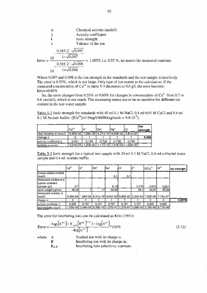
a
'Y I z
92
Chemical activity (moleIl) Activity coefficient lonic strength Valenee of the ian
0.585·22 .J0.097 10 1 +.J0.097
Error = ------;:::===_ 1.0055, Le. 0.55 %, no matter the measured contents. 0.585·2 2 .J0.ö98
10 1+.J0.098
Where 0.097 and 0.098 is the ian strength in the standards and the test sample respectively. The error is 0.55%, which is not large. Qnly type of ian matter in the calculation. If the measured concentration of Ca2+ in table 5-3 decreases to 0.6 g/l, the error become: Error=0.60%
So, the error changes from 0.55% to 0.60% for changes in concentration of Ca2+ from 0.7 to 0.6 (moleIl), which is not much. The measuring seems not to be so sensitive for different ian content in the test water sample.
Table 5-2 lonic strength for standards with 40 ml 0.1 M NaCI, 0.4 mI 0.01 M CaCI and 0.4 ml 0.1 MAcetate buffer. ([Ca2+]=3.9mgIll40080mglmole = 9.8·10-\
ion Ca2+ H+ OH- Na+ cr strength
real molaritv m (moVIl 980E-05 158E-05 631E-10 9,80E-02 981E-02 charge z 2 1 1 1 1 0098 activity caefficient Yl 0327 0,756 0756 0756 0,756 aclivitv a (malm 3,21E-05 120E-05 4,77E-10 7,41E-02 7,42E-02
Table 5-3 lonic strength for a typical test sample with 20 ml 0.1 M NaCI, 0.4 mI collected water sample and 0.4 ml Acetate buffer.
Ca2+ H+ OH- Na+ cr K'
Known added content mol/I) 0,1 0,1
Measured content in a typical collected sample (gilJ_ 0,7 0,13 0,475 atom weiQht (o/mol) 40,08 1 17 22,99 39,1 measured molarity m (moVI) 3,36E-04 1,58E-05 6,31E-10 9,63E-02 9,62E-02 2,34E-04 charoe z 2 1 1 1 1 1 activity coefficient "Ii 0,329 0,757 0,757 0,757 0,757 0,757 real molaritv (mol/l) 1,02E-03 2,09E-05 8,33E-10 1,27E-01 1,27E-01 3,09E-04
The error for interfering ions can be calculated as Kriz (1991):
Error -lagdA n+ ]+ K A,B [B m+ f' m) + log[A n+ t 100~
-log[A n+ ] O
where A B KA,B
Studied ion with its charge n. Interfering ion with its charge m. Interfering ions selectivity constant.
(804f AI3+ ion strength I
0,012 0,001 32,07 26,98
7,20E-06 7,13E-07 2 3 0,09701
0329 0,082 2,19E-05 8,71E-06
(5-12)

93
For the standards in table 5-2: [A] = 9.8.10-5 Ca2+, [B] = 9.8.10-2 Na+ and KA,B = 0.003 Kriz (1991) and the error = -2.6 %. But the content in the standard is known, so the value set is the right one.
For the test sample in table 5-3, the ion concentrations is [A] = 3.4·10-4 Ca2+, [B] = 9.6.10-2
Na+ and KA,B = 0.003 and the error is -0.9 %. When calibrating by the standard, a volume of about 0.9 % (0.0-0.9) to low is obtained for
the test sample. A comparison with ICP AES was also permformed. The deviation when measuring with the
electrodes was usually about +/- 0-10 % (sometimes about 20 %) compared to measuring by ICP AES. The error with ICP AES is normally within the range +/- 5 % according to the test centre at the Plant ecology at Lund University.
5.4.4 Chemical analysis in concrete Only specimen 3 in experiment 2 was examined with regard to the chemical content which is
toofew. Dissolving the leached concrete in HN03 as described in chapter 5.2.4 also might have
caused certain dis solution of the aggregate. Determining the solubility of the pure aggregate compensated for this error.
5.4.5 Porosity analysis Only specimen 3 in experiment 2 was examined with regard to porosity. For porosity studies
it is important to examine such large pieces so the influence from uurepresentative sample due to the aggregate can be neglected.
For the total porosity study, one half of the specimen (about 100 cm2) and one quarter (about 50 cm2) were examined. These two parts were sliced in 5+5 slices of about 7 mm thickness. These 10 slices were examined, see chapter 5.2.5. Only one specimen is too small for a statistically safe. On the other hand, the total area of the slices from this separate specimen was large enough to get a good reliability for this specimen.
5.4.6 Mechanical properties The compression tests were made on rather few specimens. Therefore the test are probably
not totally statistically significant. The size of the samples was also much smaller then for common standard tests. But the intention was only to compare leached concrete with un-leached concrete of the same size, the same recipe, and that was cast and cured in the same way. However, larger amount of samples ought to be tested in the future to get higher statistical precision.

6 CONCRETE
6.1 Introduction
94
The concrete specimens used were of two types, leaching specimens and reference specimens, see chapter 4 for an overview. The leaching specimens were exposed to a water pressure gradient. The reference specimens lay in stagnant water without any water pressure. The leaching specimens were produced from rather normal concrete used for hydraulic structures. However,'unusually high wie ratios were used to get permeable concrete.
6.2 Cement A low alkali, sulphate resistance Portland cement with moderate heat of hydration
("Degerhamn anläggningscement) of the type CEM I 42,5 was used for all three experiments, see table 6-1.
Table 6-1 Chemical composition of cement.
Cement Oxides % Clinker minerals
Type CaO SiO, Al,O, Fe,O, K,O Na,O MgO so, CI C,S C,S C,A c.AF
Experiment 1 and 2 65.5 22.7 3.56 4.32 0.57 0.05 0.45 2.07 0.02 55.7 22.8 2.1 13.1 An~y~dbyCE~A
Period 970101·971231
Experiment 3 65.4 22.7 3.5 4.2 0.6 0.1 0.7 2.1 0.0 57.3 21.8 2.1 l3 An~ysed by CEMENTA Period 980101·981231
6.3 Admixtures and additives No admixtures or additives were used.
6.4 Aggregate The sieve curves for the different aggregate fractions used are shown in figure 1 in Appendix
6. Due to the suppliers, the compact density of the aggregate is: ./ Hardeberga quartzite 2630-2640 (kg/m3) •
./ Åstorp sand 2550 (kg/m3)
Both types of aggregate are non-porous. This leads to the same bulk density as the compact density. The size distribution of the aggregate used in the different concrete recipes is shown in figures 6-1 and 6-2. Two limiting size distributions curves for good workability and thereby good homogeneity are also shown in the figures. Generally, it can be said that the smaller size and the smoother the size distribution of the aggregate, the more watertight will the concrete be. The gradation curves used are quite normal for Swedish concrete. No optimum curve with regard to impermeability was searched for.

-~ .~ c as ::I 1:1"
"CI al III III as Il.
95
-.-A ---B ..... Sand -8mm -+ Total used aggregate 0-16mm
A and B is recomended limiting curves.
100
90
80
70
60
50
40
30
20
10
O
/ ~
/ /)' / / /
V /~ tf / ~
,... / / ~/
/ / "/ /.J V/ t'" _ ..... ~ V
0,000 0,125 0,250 0,500 1,000 2,000 4,000 5,700 8,000 16,00
Size (mm)
Figure 6-1 Size distribution for sand 0-8 mm and the total aggregate 0-16 mm for experiment 1 and 2.
-.-A ........ 8 ..... Sand -8mm
A and B is recomended 11miting curves.
100
90 -7 t'"
/ / 80
70 / / ~ ~ .~ c as ::I 1:1"
"CI al III
= Il.
60
50
/ V /"" / ./ /
/ / r' /V 40
30 / /' /' 20
10
o
/'" L v/ r'..-/ .........
_.-.-I r---~ V
0,000 0,125 0,250 0,500
/r
1,000
Size (mm)
2,000 4,000
Figure 6-2 Size distribution for sand 0-8 mm for experiment 3.
5,700 8,000

96
6.5 Mixing and curing water Ordinary municipal tap water was used both as mixing water and curing water.
6.6 Recipes The recipes for the different types of concrete that were used are shown in tables 1 to 5 in
appendix 6.
6.7 Casting The concrete was mixed in an ordinary laboratory concrete mixer. Cement and aggregate
were mixed frrst for about 3 minutes. Then water was added and the mixing continued for about 3 minutes more.
For the leaching specimens, the concrete was cast in steel cylinders (figure 6-3) placed on fibreboard and vibrated on a vibrating table for approximately 15-20 seconds. The steel cylinders were the same cylinders as were used later in the leaching test. The thickness of the specimen was adjusted for the correct value using a piece of wood.
= 155 and 45 mm
Figure 6-3 Casting of the leaching specimens.
The reference specimens were cast in 300 mm long steel tubes with diameter 150 mm. The concrete cylinders were later cut in 50 mm slices.
After about 24 hours in plastic bags, all the specimens and cylinders were unmolded.
6.8 Curing The experimental specimens were divided in three groups: ,/ Experiment 1 was a feasibility study to see if the test equipment worked and to see which
concrete quality to use. The concrete quality was virgin (undried) w/c 0.8 concrete. ,/ Experiment 2 was an outcome of experiment 1 and included specimens with much higher
permeability. Virgin concrete with w/c 0.8 and 1.3 were used together with late-dried specimens with the same w/c ratios.
,/ Experiment 3 was an attempt to use a more normal curing, early-heating, and to study the lower w/c ratio of 0.6.
A more precise specification over the casting and curing conditions are shown in tables 6 to 9 in appendix 6. See also chapter 4 for an overview.
After the pressure and reference specimens were unmolded, they were either put in a water storage tank (experiment 1 and experiment 2) or put in plastic bags and in an oven (experiment 3). The specimens, which went to the water storage tank, were later, either put in the pressure

97
cells (virgin specimens) or dried in an oven (late-dried specimens). The specimens that were dried were water saturated by vacuum treatment followed by water absorption before they were mounted in the pressure cells.
The specimens that were put in oven directly af ter unmolding (experiment 3), were stored in the same plastic bags in room temperature until they were exposed to water pressure. Before the specimens were mounted in the pressure cells, they were water saturated by vacuum treatment followed by water absorption. The virgin (never-dried) specimens were assumed to be water saturated without vacuum treatment.
The curing water was saturated with lime to prevent any leaching of lime from the specimens during the curing.

98
7 RESULTS OF EXPERIMENTAL WORKS
7.1 Permeability All results from the leaching test regarding water flow permeability are shown in Appendix
7. A summary is shown be10w in figures 7-1 to 7-7. Generally, the water flow was different for different concrete qualities (wie 0.6, 0.8 and 1.3)
and for different curing histories (virgin, early-heated and late-dried) . ./ Virgin = never dried eonerete, see a short description in chapter 4 and 6.7 . ./ Early-heated = heated in oven directly after un-molding, see chapter 4 and 6.7 . ./ Late-dried = virgin specimens that was dried after 6.5 months, see chapter 4 and
6.7. The results show three different water flow pattern; a constant water flow, an accelerating
water flow or a retarding water flow. Observe that the last observed flow of water for each specimen in the figures, is no final water flow, but the water flow at just that time when respective specimen were taken out of the pressure cell.
Below a summary is made of the observed effect of w/c-ratio and pre-curing history, see also figure 7-7 for an schematic over-view. .
The water flow for the specimens with virgin w/c 0.8 (figure 7-1 and specimens 2 and 5 in figure 7-2) was constant of about 10-11 m%. However, one of the specimens had an increased water flow of 100 times after some time, to about 10-9 m3/s.
The water flow for the specimens with late-dried w/c 0.8 (specimens 1,3 and 4 in figure 7-2) was constant of about 10-9 m%, which is approximately 100 times larger compared to the virgin state. However, one of the specimens had a further increased water flow of 100 times af ter some time, to about 10-7 m3/s
The water flow for the specimens with virgin w/c 1.3 (specimens 10 in figure 7-2) was initially constant of about 10-9 m% for the one tested specimen, which is 100 times higher than virgin concrete with wie 0.8. Later the flow increased 100 times to about 10-7 m3/s.
The water flow for the specimens with late-dried wlc 1.3 (specimens 6-8 in figure 7-2) was constant of about 10-8 m3/s, which is approximately 10 times larger compared to the virgin state. Later, the water flows for all these specimens increased about 100 times to about 10-6 m3 Is.
The water flow for the specimens with early-heated wlc 0.6 was initially about 0.5 to 1.010-9 m3/s for the specimens with a diameter of 150 mm (specimens 1,5-7 in figure 7-3), but rather fast it decreased 10 times down to about 10-10 m3/s. After 12 000 hours, the water flow had decreased about 100 times to 10-11 m%. The specimens with a diameter of 45 mm (specimens 20-30 in figure 7-4) had the same development, but only 30% oftheflow of the larger specimens, if converted to the same diameter.
The water flow for the specimens with early-heated wlc 0.8 was initially about 0.5 to 1.0 10-9 m% for the specimens with a diameter of 150 mm (specimens 1,5-7 in figure 7-3), but rather fast it decreased 10 times down to about 10-10 m%. After 12 000 hours, the water flow had decreased about 100 times to 10-11 m3/s. The specimens with a diameter of 45 mm (specimens 31-36 in figure 7-5) had the same development, but only 50% of the flow of the larger specimens, if converted to the same diameter.
Thus, the water permeability differed by about 100 000 times from the lowest initially water flow value of virgin concrete with wie ratio of 0.8, to the highest flow after about 30 days in the late-dried concrete with wie ratio of 1.3.
The early-heated concrete had permeability that was about 50 times higher compared to the virgin eonerete, but after some time it was reduced to about 5 times as high as the virgin eonerete, probably by self-healing.
When the water flows increased for some concrete specimens, they were dismantled to see if there were any visual changes. At the upstream face of the concrete specimens, small brown

99
areas were always observed. The brown areas consisted of compounds containing Al, Fe, Si and some Ca, probably residual parts of leached C-S-H and AF phases. In the centre of the brown areas, small pipes leading into the concrete were observed. Probably these holes were the socalled mainflow pipes, in which the main water flows had occurred.

100
-'-spec.1
--'-spec.3
---spec.5
-+-spec.7
-<>-spec. g
~Exp 1 w/c 0.8 virgin, mean q spec. 1-10
1,OE-09 .,--------------------1
{ 1,OE-10 +--'1\----.,..".==,-------------1
.,. ~
:;::
!1,OE-11
~ '" c: 'i! c
-+-spec.2
-spec.4
-9-spec.6
-6-spec.8
--spec.10
1,OE-12 +-1\--+---+1--------------------------------1
1,OE-13 -1-----,-------,----..,-------,----,-------,.-------,.-------1
o 200 400 600 800
Time (h)
1000 1200 1400 1600
Figure 7-1 Water flow in experiment l: virgin concrete wie 0.8 (spec. 1-10). The mean flow for the same specimens is also

101
given.
---spec. 1 -+- spec. 2 ...... spec. 3 -spec. 4 --spec. 5 -a- spec. 6 -+-spec. 7 ....... spec. 8 -e-spec. 10
1,OE-06 r~;;:;:::::l6~to~1~b~a~r~--,-----rr---:;==~~!!:=:=~~--r
1 ,OE-O? +--'--#fL--IIII~,"""-----+-----+l
{ 1,OE-08 +J!I'-,;IIJ\--.P .... -t-II----+------H
~ ;::
S 1,OE-09 ~ .. ~
4
~ 1,OE-10
1,OE-12 -J-----+-----+-----+-----+-----+------J----' o 2000 4000 6000 8000 10000 12000
Time (h)
Figure 7-2 Water flow in experiment 2: virgin concrete wie 0.8 (spec. 2 and 5), late-dried w/c 0.8 (spec. 1,3 and 4), virgin w/c 1.3 (spec. 10) and late-dried w/c 1.3 (spec. 6-8). Observe that the water pressure for specimens 1, 6-8 and 10 was reduced from 6 to 1 bar because of large water volumes.
---spec.1 -+-spec.5 ...... spec. 6 -spec. 7 --spec. 8 -a-spec. 9 -+-spec. 10
1,OE-08.--r---,r----,---.,.-----,-----.,----!
1,OE-11 +----l---+---+-----1~--_+---+---+_--_+--._I
1,OE-12 +----t----t----+---......,r----+----J----+----+----f o 1000 2000 3000 4000 5000 6000 7000 8000
Time (h)
Figure 7-3 Water flow in experiment 3: early-heated concrete w/c 0.6 (spec. 1,5-7), earlyheated w/c 0.8 (spec. 8-10).
9000

---Spec.20 -SpeC.23 ....... Spec.26
""*"" Spec. 29
102
-+-Spec.21 -+-Spec.24 -6-Spec.27 ...... Spec.30
1,OE-09 -,-----,--....,---,---,--..,..----,r--.... -t
-6-Spec.22 -e-Spec.25 -<>-Spec.28 ~w/c 0.6 mean q spec. 20-30
.. 1,OE-10 +-----r---t--+--+---r---t---t--t i r:r
~ ;;::
a; 1,OE-11 t;j ~
& f~~~~~~~S:~~~~~~~~~~~~~~~~~!i ~ '! Q 1,OE-12
1,OE-13 +----f---/---!---+---f---1r---f---+----f---/---+++----; o 500 1000 1500 2000 2500 3000 3500 4000 4500 5000 5500 6000
Time (h)
Figure 7-4 Water flow in experiment 3: early-heated concrete wie 0.6 (spec. 20-30). The mean flow for the same specimens is also given.
___ Spec. 31 -+-Spec. 32 -6-Spec. 33 - Spec. 34 --Spec. 35 --El- Spec. 36 ~w/c 0.8 mean q spec. 31-36
1,OE-10 ,---.----;---,---..,---,-----,---r---,---,---,..---;--,
i r e 1,OE-12 Q
1,OE-13 ~==+==~==t===I--_l_---+--t_--+--___4--_I_-_+-~ o 500 1000 1500 2000 2500 3000 3500 4000 4500 5000 5500 6000
Time (h)
Figure 7-5 Water flow in experiment 3: early-heated concrete w/c 0.8 (spec. 31-36). The mean flow for the same specimens is also given.

____ Exp 1 w/c 0.8 virgin. mean q spec. 1-10
....... Exp 2 w/c 0.8 late dried, mean q spec. 1,3,4
--Exp 2 w/c 1.3 late dried, mean q spec. 6-8
103
-+- Exp 2 w/c 0.8 virgin, mean q spec. 2,5
- Exp 2 w/c 1.3 virgin, q spec. 10
-tI- Exp 3 w/c 0.8 early dried, mean q spec. 8-10
1 ,OE-Ol +-----o~r+---_3ilr-It_---+---_+--___I
1,OE-12 +_----+----f----+----+---~----+_---_I_---_+----l
O 1000 2000 3000 4000
Time (h)
5000 6000 1000 8000
Figure 7-6 Mean water flow f..l[q] for experiment 1 (specimens 1-10), experiment 2 (specimens 1-8 and 10) and experiment 3 (specimens 6-10).

Water flow m3/s 10-6
..-Exp. 2late-drled W/rtf.3
I •
10-9 • J'"
104
l tf +
Exp. 2 virgin wlc 1.3 / ,,-• ",. ~XP. 2late-dried wie 0.8 --
'" Exp. 3 early-heated
"-- r' Exp. l virgin wlc 0.8 •
10-\2
Figure 7-7 Aschematic picture over the flow of outlet water in experiments 1-3.
7.2 Chemical analysis of the drainage water
7.2.1 General
Time
The test procedure and the concrete specimens are described in chapter 4, 5 and 6. The water that was pressed through the concrete specimens, here called the drainage water (sometimes called the outlet water), was analysed regarding its chemical contents. Only data from experiment 2 (late-dried w/c 0.8 and 1.3) is shown. In this chapter an overview of the result is given. The results of the chemical analysis are also shown in appendix 7-4 to 7-7.
The experiments show three types of leaching behaviour: ./ Leaching in homogenous concrete with constant flow . ./ Leaching in homogenous concrete with increasing water flow . ./ Leaching in homogenous concrete with decreasing water flow.
As mentioned in chapter 7.1, there was a constant drainage water flow in specimens with low w/c ratio and for virgin (non-dried) specimens. Increasing water flow appeared for high w/c ratios and for late-dried specimens. Finally, the decreasing water flow appeared for the earlyheated specimens. Some ions diffused upstream, against the water flow, towards the inlet water. This is treated in chapter 7.3.

105
7.2.2 Leaching of Ca When the water flow was constant, the concentration of leached calcium in the drainage
water was also constant with a mean value of about Il[Ca] = 0.6 g per litre drainage water, (figure 7-8). The leaching rate of Ca expressed as the product of the water flow and the concentration in the drainage water; I,m3/s·kglm3 = kg/s, was also constant because of the constant flow of water.
2,5 .-------------~~~~~-------------. c CI)
E 2+------ .,--'=---'--------II Staple chart of the ·u CI)
~ 1,5 -t------~"""'-
ö l!! 1 CI) .Q E 0,5 +---+-::::I c
0+----'--,-
concentration of Ca for specimens 1 to 5.
- Adjusted distribution of the concentration of Ca for specimen 1 to 5
<0.5 0.5 to 0.55 to 0.6 to 0.65 to >0.7 0.55 0.6 0.65 0.7
Concentration of Ca (gli) Figure 7-8 Variation in Ca concentration in the drainage water for five specimens of virgin and late-dried w/c 0.8 eonerete, before any rapid increase in water flow occurred.
When the water flow was increasing, the concentration of calcium in the drainage water decreased from the above mentioned 0.6 glI down to as lowest measured 0.005 gJl. The leaching rate expressed as kgls was however quite constant.
When an accumulated water flow of about 1 to 10 litres had percolated each specimen, the concentration of Ca began to decrease in the drainage water, see figures 10 to 12 in appendix 7-4. A specimen of the size <1>155 (mm)*50 (mm) has an initial content of cement of:
w/c 0.8 expo 1 and 2: Illc = V*C = 1t·0.1552/4·0.05 m3·241 kglm3 = 0.227 kg cement w/c 1.3 expo 2: Illc = V*C = 1t·0.1552/4·0.05 m3·158 kglm3 = 0.149 kg cement
1 litre percolated water for these two concrete types correspond to: w/c 0.8 expo 1 and 2: 1/0.227 = 4.41/kg cement wie 1.3 expo 3: 1/0.149 = 6.71/kg cement
When the water flow was decreasing, the concentration of calcium in the drainage water was constant, but a little bit higher than when the water flow was constant, 0.8 to 1.2 g Ca per litre drainage water. The leaching rate expressed by kgls decreased due to the decreasing flow of water.
The residual content of Ca in the specimens, decreased by rates that differs only a little among the same type of concrete/curing method.

106
7.2.3 Leaching of K and Na Both the concentration (kg/l) and the leaching rate (kg/s) of K and Na in the drainage water
decreased when water was pressed through the specimens. This was the case for all the three types offlow pattems; constant, decreasing and increasing water flow. The concentrations began to decrease when approximately O.llitre had flown through the specimens.
7.2.4 Leaching of S The initial concentration of leached sulphate in the drainage water was quite high (0.02 g/l).
It slowly decreased during the test.
7.2.5 Leaching of Mg, Fe and Si The leaching of Mg was typically about 0.01 to 0.1 mg per litre drainage water. The initial
concentration of Mg in the cement was according to the cement supplier about 0.45 % MgO per kg cement, i.e. approximately about 600 mg/specimen (e.g. for specimen 2: 0.0045*24.31 g/mole/40.31g/mole*245*106mg/m3*1t*.155A 2/4*0.05 m3 = 630 mg/specimen). The maximum observed leaching of Mg occurred in specimen 7 (late-dried wie 1.3) and was about 1 mg Mg, which is a fairly low value.
The leaching of Fe was typically about O.Olmg per litre drainage water. The initial content of Fe was according to the cement supplier about 4.32 % Fe203 per kg cement, i.e. approximately about Fe(s) = 0.0432*55.85*2(g/mole )/159.7 (g/mole )*245* 1Q6(mg/m3)*1t* . 155A2/4*0.05(m3) = 6900 mg/specimen for the w/c 0.8 specimens. The maximum drainage appeared in late-dried specimen 1 and was about 17 1*0.01 mg/l= 0.2 mg, i.e. 0.2/6900, which is a very low value.
7.2.6 Changes in pH The pH value of the drainage water decreased when its content of K+ and N a + decreased. It
decreased from about 13.2 -13.4 to about 12.5, corresponding to the pH-value of a saturated Ca(OHh solution. For the very permeable specimens where much water was percolated, the pH decreased even more. The lowest observed value was 10.25 in specimen 1, experiment 2.
7.2.7 Summary There were three types of leaching behaviour (figure 7-9) that were strongly correlated with the concrete type (w/c 0.8 or w/c 1.3) and the curing history (virgin, late-dried or early-heated). As described in chapter 7.1, the water permeability was different for these concrete types. When the water flow was constant, there was a constant concentration in the drainage water of leached Ca of about 0.7 to 1.2 g/l for the early-heated specimens, and about 0.6 g/l for the rest. The concentration of K and Na in the drainage water rapidly decreased for all specimens. Due to the decrease of K and Na in water, the pH-value in the drainage water fell somewhat at the beginning. When the water flow increased, especially when it increased rapidly, there was a rapid decrease in the concentration of Ca and pH. The concentration of S had a slowly decreasing rate, more or less unaffected by the water flow.

:ontent in the rainage water.
~13.3 \ \
107
[Ca'+] in the drainage water ~O.6 to 1.1 gli
\ ~12.5 ''-, ~ pH in the drainage water
\ '" [K+] and [Na +] in the ''-,-\"" drainage water '/
\ '---- ------~ - . - ":--"::"A-. I" ~ ._ . ..,
[S] in the drainage water .,.,' - • _ • _. ~ •• -_"~
Drainage water flow
-----.-
Accnmulated now ofwater (m3)
Figure 7-9 Aschematic picture over the effect of leaching on the ion content and pH-value of the oudet water in experiment 1-3.
7.3 Chemical analyses of the water at the upstream face The test procedure and the tested concrete specimens are described in chapter 5 and 6. As mentioned before, the inlet-water leading to each specimen, was de-ionised. The whole
upstream surface of each concrete specimen was exposed to this pure water. Because of the large gradients in concentration of ions between the concrete surface and the water, the diffusion of ions from the concrete surface to the purified water was probably quite large. The dissolved ions from the specimens made ilie inlet-water less de-ionised as it was meant to be. To maintain pure water condition water was flushed out from the inlet side at every measurement occasion. But, by doing so, the dissolved ions were also flushed away. Even if ilie concentration was low, the diffusion upstream should be inc1uded in the total loss of leached material from the concrete specimens.
Between every flushing, the inlet-water was again gradually refilled by dissolved ions from the concrete. No systematic measurement of the ion concentration of the inlet water was made. Only a few measurements of the pH-value and the concentration of Ca2+ in the out-flushed water were performed. By this, a rough estimation was made of the removed ions due to diffusion in the upstream direction.
In figure 7-10 an estimation of the amount of Ca-ions leached upstream is shown. It is based on measurements of out-flushed water from specimens 6 to 10 in experiment 3. At every measurements of water flow, about 2 litre of water was flushed per specimen of size <\>155 mm and about 0.3 litre per specimen of size <\>45 mm.
The diffusion upstream of C~+ decreased from initially about 0.03 g/l for the first 2 litres of collected water per concrete specimen, to about 0.01 g/l at 400 hours (see figure 7-10). At 400 hours to 500 hours the concentration was measured in three different samples, in the first litre

108
(O.OS glI), in the second litre (0.02 g/l) and in the third litre that was flushed (0.008 g/l). At 8S0 hours the concentration was measured for two different samples, for the frrst 0-1.S litre (0.03 g/l) and for the next 1.S -3litre (0.01 g/l) that came out by the flushing. This shows that it was concentration gradients in the inlet water, from the specimens and in the upstream direction in the steel pipe system.
In figure 7-11, the measured pH values from the inlet water that was flushed from specimens 6 to 10 in experiment 3, is showed.
Dissolved Ca2+ in upstream water
___ Ca gli from 0-1 liter sample volume _Ca gA from 1 -2 liter sample volume "'-Ca gli from 2-3 liter sample volume -Ca gli from 3-4 liter sample volume ..... Ca gA from 0-1.5 liter sample volume --Ca gli from 1.5-3 liter sample volume -e-Ca gli from 0-10 liter sample volume
0,07
0,06
~ 0,05
3 0,04
'ö 'E 0,03
! 8 0,02
0,01
o
GI..
o
"\ If---l "' r--..... 100 200 300
J\ i I i
/ \ I , / \
, i i
~ I lIC
... I
T • I ,---- l , l
400 500 600 700 800 900 1000
Exposure time (h)
Figure 7-10 Measured content of Ca2+ in the out-flushed water from the inlet side of specimens 6-10 in experiment 3.

109
pH in upstream water
..... pH from 0-1 liter sample volume ....... pH from 1-2 liter sample volume ""'-pH from 2-3 liter sample volume __ pH from 0-1.5 liter sample volume -e-pH from 1.5-3 I~er sample volume -+-pH from 0-2 liter sample volume -'!'-pH from 2-4 liter sample volume ""*"pH from 4-6 liter sample volume -e-pH from 0-10 liter sample volume
12,2
12
11,8 ,,-:-~ ...
~ 11,6 "\ ~ .. \ .So
+ 11,4 J:
'ö 11,2 c el) 11 c o 10,8 (.)
10,6
10,4
10,2
o
\ ..... i ('GJ(/7L..J 1-'\ /-- \ ~ 1
'At
1000 2000 3000
Exposure time (h)
4000
" -J V
5000
Figure 7-11 Measured content of W (PH) in collected water from the upstream face of specimens 6-10 in experiment 3.
6000
Some brown, soft areas were always observed at the upstream face of concrete specimens having a rapidly increased permeability (see chapter 7.1). A chemical analysis of this brown substance was performed. The result is shown in table 7-1. The results can not be treated quantitatively because a certain amount of the brown material was analysed together with some of the upstream water. Therefore, the unit mg/litre can only be regarded as an indication of which elements the brown powder consists of and of the proportions of elements.
Table 7-1 Measured content in mg of element per litre of water in the sample. The sample was taken from observed brown areas in the upstream face of specimen 7.
Water sample from experiment 2, specimen 7
Al 15.2
Ca 39.2
Fe K 93.0 0.9
7.4 Chemical analysis ofthe leached concrete
Na s 0.7 4.0
A chemical analysis was performed for one specimen; specimen 3 in experiment 2.
Si 20.2
The contents of different residual elements in flve slices taken from the leached concrete were examined. The result is shown in table 7-2 and in flgure 7-12. The chemical analysis was made by the method described in chapter 5.2.4.When the slices were dissolved in the HN03, a solution and a solid rest at the bottom were obtained.
The dissolved elements in the solution probably emanated from the cement paste, but also to some extent from the aggregate. The solid rest probably emanated from the aggregate, but also to some extent from the cement paste.

110
In order to estimate how much of the dissolved elements that came from the paste and how much that came from the aggregate, a second study of only the aggregate was performed. The second study was performed in the same way and with the same type and amount of aggregate that was used for the concrete specimen 3. See table 7-3.
Table 7-2 The chemical composition of the dissolved matter from one half (piece 1) of specimen 3 in experiment 2. The specimen was cut in 5 slices. Slice 1 is elosest at the downstream face and slice 5 elosest at the upstream face. The position of the slices is shown in figure 7-12. The content of elements is in mg element per mg of the total slice. The aggregate content is in weight percent of the total slice weight.
Measured Measured Measured Measured Measured Measured Measured Measured Measured Measured residua! residua! residua! residua! residua! residua! residua! residua! S residua! residua! Alpiece Capiece Fe piece Kpiece 1 Mgpiece Mnpiece Napiece piece 1 Si piece 1 solid 1 1 1 (mg/mg) 1 1 1 (mg/mg) (mg/mg) piece 1 (m~mg) (mg/mg) (m~mg) (mgImg) (mgImg) (m~mg) (% )
Slice 1 6,460 44,756 11,466 1,251 1,128 0,315 0,225 1,507 0,105 82,3
Slice 2 5,419 37,550 10,767 1,197 1,014 0,259 0,191 1,247 0,089 83,5
Slice 3 5,794 43,461 10,142 1,189 0,968 0,278 0,191 1,704 0,092 83,5
Slice 4 6,129 45,242 10,526 2,222 1,205 0,298 0,178 1,771 0,157 82,6
Slice 5 6,235 41,375 11,550 1,285 1,266 0,359 0,247 1,588 0,127 80,6
Table 7-3 The chemical compositian of the dissolved matter from the same aggregate that was used in table 7-2 after dissolution in HN03 acid. The aggregate content is in weight percent of the total slice weight.
Measured Measured Measured Measured Measured Measured Measured Measured Measured Measured residua! residua! residua! residua! residua! residua! residua! residua! S residua! residua! Alpiece Capiece Fe piece Kpiece 1 Mgpiece Mnpiece Napiece piece 1 Si piece 1 aggregate 1 1 1 (mgImg) 1 1 1 (mgImg) (mgImg) piece 1 (mgImg) (mgImg) (mgImg) (mgImg) (m~mg) (~ (% )
Sand 4,271 3,708 13,930 0,082 1,439 0,291 0,000 0,031 0,022 94,90 0-8 grave1 1,602 0,620 2,087 0,644 0,187 0,025 0,245 0,158 0,000 98,72 8-16

111
Dissolution of five slices from specimen 3, experiment 2. Water pressure
100,0
.~ "iii ..c l;l al -tO,O .!: .~ J!l"iii c el al E 5"i:n "iii E1,0 --' o ..c Öl
~ 0,1
0,0
.11.
11+
/ ~ - ""-
--2 3
Slice
_\ ~
85 '2f ~ iii
84 :s ö ~
83 'E, .~
S 82 &
l!! el
~
~ecel
. ~",;:, >. ,iB Slice S
Slice 1
....... Measured residual Al plece 1
-+-Measured resldual Ca piece 1
....- Measured residual Fe piece 1
- Measured resldual K plece 1
...... Measured residual Mg piece 1
-e-Measured residual Mn piece 1
\ 81 -+- Measured residual Na piece 1
4 80
5
-å- Measured resldual S plece 1
-+-Measured residual SI piece 1
~ Measured residual Solid plece 1
Figure 7-12 The chemical composition of the dissolved matter from one half (piece 1) of the specimen 3 in experiment 2. Slice 1 is c10sest at the downstream face and slice 5 c10sest at the upstream face. Observe the log scale.
7.5 Porosity
7.5.1 Total porosity Only one specimen was analysed for porosity after terminating leaching test, specimen 3 in
experiment 2 (late-dried w/c 0.8). The porosity was measured by the method described in chapter 5.2.5. The porosity after the specimen had been leached for 306 days is showed in figure 7.:13. Piece 1 is one half of the specimen and piece 2 is a quarter ofthe specimen. The specimen was also cut in 5 slices, slice 1 c10sest at the outlet surface and slice 5 c10sest at the inlet surface.
From the measurement of the porosity, also the density was obtained, see figure 7-14.

0,300
0,250
c;) 0,200
.€ ~ -;:: 0,150 .'1::
2 o
lI.. 0,100
0,050
0,000
112
Experiment 2, specimen 3: Porosity
J -~:: lA Slice'
...-iI- /: I .~ ... ~ -- 17 I
..... Measured resi dual total porosity Pc piece 1
-+-Measured resi dual total porosity Pc piece 2
I i
1 2 3 4 5
Slice (1 =downstream face, 5=upstream face)
Figure 7-13 Porosity of the leached specimen 3 in experiment 2. The initial total porosity is assessed in chapter 8.4, see figure 8-8, where also the measured residual total porosity of piece 1 in the above figure is shown.
2800
2700
2600
i' 2500 ~ E -;:: 2400
-I ;:; 2300
lI..
2200
2100
2000
Experiment 2, sample 3: Density
..... . ....-- --~'" ~
2 3 4
Slice nos (1=downstream face, 5=upstream face)
" 5
-II- measured residual compact density (kg/m3)
-+- measured residual dry bulk density (kg/m3)
Figure 7-14 The compact density and the drybulk densityforpiece 1 of the specimen 3, experiment 2.

113
7.5.2 Pore size distribution The pore-size distribution of specimen 3, experiment 2 (late-dried w/c 0.8) was studied. The
porosity after the specimen had been leached for 306 days is shown in figure 7-15. The distribution was measured by the method described in chapter 5.2.5. Unfortunately the measurement was interrupted when the air pressure was changed to 100 bar because the air was flowing so rapidly in the test cell that the small concrete slices were pulverised.
Pore size distribution
0,070 -,---------.,.----------,---1
0,060 -t----------t----------j----I
0,050 +----------1-\---------+----/ (öl E i 0,040
.~ ~ 0,030 -t------------1It\:--+---------j------... o D.
0,020 +----------+--'I~,____------+-------
0,010 -t---------.-~hl__-------t-------
SliceS
___ Slice 1
-+-Slice2
-Ir-Slice 3
-Slice 4
..... Slice5
0,000 -I---------1--~I,:lii~~~e==*==~-4I~--_4 1,OE-08 1,OE-07 1,OE-06 1,OE-05
Circular pore diameter (m)
Figure 7-15 Pore size distribution in the leached specimen 3, expo 2. The pore size distribution is not complete due to the problem described above.
7.6 Mechanical properties
7.6.1 Compressive strength Small cylinders were drilled from five leached specimens coming directly from the leaching
test. The cylinders were all water saturated. The same number of cylinders were drilled from reference specimens. All cylinders were tested in a compressive machine. Some of the leached cylinders had lower compressive strength than the un-Ieached cylinders.
Specimens 1, 3, 6, 8 and 10 from experiment 2 were strength tested directly after they were taken out of the test cell. See table 7 in appendix 6 for the time history for the specimens. The un-Ieached reference specimens had the same history, but were stored in lime-saturated curing water, without any pressure gradients during the same time as the comparing specimens were leached.
Specimens, which have had a large increase in water-flow during the water-pressing test, were in a very bad shape after the leaching test. Specimen no 7 fell completely apart when trying to drill cylinders. So from this specimen, no cylinder was available. Also one drilled cylinder from specimen no 8 was discarded since many small pieces fell from that cylinder. Many of the other cylinders also obtained minor damage during drilling. But after grinding, reasonable fine test surfaces were obtained.
In chapter 7.1, the observation of small brown areas in the upstream face of same specimens was mentioned. In these brown areas, it was also observedflow pipes leading into the specimen,

114
where the main water flow evidently had taken place and at the same time probably leached solid material. It was observed during the compressive test, that cylinders with many such brown areas and flow pipes, had lost much more of their strength. Around some larger flow pipes leading through the specimens, so much hydration products were lost, that the concrete no longer had any cohesion. Cylinders from leached specimens without such brown areas and flow pipes had almost the same strength as the reference specimens. So the influence of leaching on the compressive strength was very much a local effect.
In table 7-4, figure 7-16 and in appendix 7-8, the concrete compressive strength is shown. The value "29 MPa" for the unleached specimen 3 seems too low, compared to the strength of the other specimens, hut there is unfortunately no explanation to this.
Table 7-4 Compressive strength for un-Ieached and leached concrete specimens from experiment 2.
Specimen
1 (virgin w/c 0.8) 3 (late-dried w/c 0.8) 6 (late-dried w/c 1.3) 8 (late-dried w/c 1.3) 10 (virgin wie 1.3)
Compressive strength (Mpa) Un-Ieached specimen Mean Stddev 46 0.8 29 3.5 19 0.3 18 5.0 21 7.2
Leached specimen Mean Stddev 36 14.8 33 16 4.7 12 18 2.5
Measured compressive strength fcc for piece 3, specimen 3, expo 2.
50,00
45,00
_ 40,00
:. e 35,00 ;; g' 30,00
~ 25,00 ~ .;: 20,00 l!! ~ 15,00
8 10,00
5,00
0,00 o
I~ot leached wlc 0.8: mean = 36.1 Mpa
IstddeV = 9.6 MPa
I~eached w/c 0.8: mean=3S.1 MPa
!StddeV = 10.6 MPa
0,2 0,4
/' I 1--1 i
i
I { • I \ I
Mean values of fcc
1- l\ / i ---Not leaohed wlc 0.8
I -.- Leached wlc 0.8
! ~ /.". ---.-Not leached wlc 1-.3
I Not leached wie 1.3: I --../\ ( :. i --- Leached wlc 1.3 l can =19.3MPa I ~ stddev = 4.3 MPa
!;eaChed wie 1.3: 1...1 "' mean = 15.8 Mpa
Istddev = 3.6 MPa I
0,6 0,8 1,2 1,4
wlc ratio
Figure 7-16 Mean value and standard deviation of the compressive strength for piece 3 coming from specimen 3 in experiment 2.

115
7.6.2 Elastic modulus From the figures in appendix 7-8 over measured data of applied stress and deformation, the
modulus of elasticity E is calculated and presented in table 7-5.
E=..:la·U&
Where E ..:la
L &
= modulus of elasticity (pa) = a change in applied compressive stress for a certain change in
deformation &. Obtained from the steep part of the measured curves in appendix 7-8. (pa)
= the length of the tested cylinders (m) = the deformation change for the change in stress ..:la (m)
Table 7-5 Elastic modulus for un-Ieached and leached specimens.
Specimen
1 (virgin w/c 0.8) 3 (late-dried wie 0.8) 6 (late-dried w/c 1.3) 8 (late-dried w/c 1.3) 10 (virgin w/c 1.3)
Elastic modulus E (Gpa) Un-Ieached specimen ~ean Stddev 3.4 0.9 4.5 2.7 1.2 0.2 1.4 0.4 1.8 0.2
7.7 Dissolving rate of Ca(OHl2 in de-ionised water
Leached specimen ~ean Stddev 2.4 0.8 19.7 0.7 0.1 0.6 1.1 0.4
(7-1)
A simple test of the dis solution of Ca(OH)2 in de-ionised water was done, see also chapter 5.2.7.
Figure 7-17 shows the result. hritially the solution was not stirred, but af ter 240 seconds a magnetic stirrer was placed in the solution. Without stirring, an asymptote was reached at approximately 0.4 g of dissolved Ca2+ per litre, i.e. 0.01 mol/l. The rest of the Ca(OHh remains un-dissolved. When beginning to stir the solution, the reaction re-started, reaching 0.46 g Ca2+/l. The re action rate was rapid, especially at the beginning when the water was pure.

13,23
11,34 ,..
9,45
7,56 ::t: Do
5,67
3,78
.... I
hl t
1,89
o O 100
116
Dissolving of Ca(OH)2
-ll-Measured pH -+-Measured Ca(aq) g/I
200
.~ .. .-A ~
!
i~s::;:c tlrrer
i ! i i i
i i
i 300
Time (s)
- -......- "T
400
- -
500
0,5
0,45 'tJ
0,4 Iii easS
0,35 ~ 5 :g~
0,3 UI "ö iii UI
0,25 .g .5 'iii~
0,2 ! Ö o ...
0,15 'I: ii 11)'1:
0,1 ~ 8 (.)
0,05
O
600
Figure 7-17 Experimental result of dissolving powder of Ca(OH)2 in de-ionised water.

117
8 DISCUSSION OF RESULTS AND MODELLING OF THE LEACHING PROCESS
8.1 Introduction In the experiments presented in this report, pure water under pressure was applied to the
upstream face of the concrete specimens. On the outlet side, drainage water without any pressure was coming out of the specimen.
The experimental results show that pure water percolating through concrete has an ability to dissolve hydratian products, mainly Ca(OH)2, and also to carry the dissolved ions out of the specimen. The transport of the dissolved ions can occur as diffusion upstream to the bulk of pure water at the inlet side or as convection in a downstream direction by the flow ofwater. Depending on the w/c ratio and the curing history, leaching develops in different ways. Mature concrete with a high hydratian ratio or mature concrete that was dried (late-dried) was more porous and permeable. If the specimens were early-heated, the water permeability became high at the start but it quickly decreased due to restarted hydratian and self-healing.
In the high-permeable concrete, water seems to have flowed in a rather few, distinct flow pipes. In these pipes, water had dissolved solids, mainly Ca(OHh and thereby grew wider. Therefore the water flow increased further, which caused more leaching in a accelerated process. Finally, the pipe walls became so exhausted in solids (lime) that the leaching rate and the water flow increased only slowly. Around these pipes the concrete became very disintegrated with almost no continuous cementitious materialleft to maintain strength and tightness.
Between the flow pipes, or in not so permeable concrete, the leaching was govemed by diffusion to the flow pipes or to the bulk of soft water at the upstream end.
The permeability is related to the number and size of the flow pipes, and the permeability is therefore increased when the flow pipes become wider in the leaching process. The leached layer at the upstream face does probably not have a big effect on the permeability.
The measured residual content of substances in the leached specimens approximately weIl corresponded to the measured ionic flow in the drainage water flow.
When the OR- ions were leached, the pH value decreased in the drainage water and probably also in the pore solution; anyhow in the main flow pipes.
The results also show that when solid material is leached, the porosity increases and the strength decreases due to less load-bearing solid material. The number of specimens that were tested with regard to strength, were however too small for really reliable results.
In the following sections, the following parameters are discussed: (i) permeability, (ii) leaching in the upstrearn face, (iii) 1eaching through the specimen, (iv) residual content of substances in the leached specimen, (v) porosity, (vi) strength.
8.2 Discussion of permeability results A number of concrete specimens (chapters 4 and 6) were exposed to water pressure and the
flow of the drainage water out of the specimens was measured (chapter 7.1). The results show that there are three different types of water flow:
vi' a constant water flow. vi' an accelerating water flow vi' an retarding water flow
A constant water flow always appeared at the beginning of the test for all specimens. The late-dried and the early-heated specimens had an about 100 times higher initial permeability than in the virgin state. Some specimens maintained a constant flow but others obtained flow that changed with time. The main reasons for a constant water flow were probably:

118
./ the test time was not long enough. If there are no self-healing effects (e.g. formation of calcite), probably all concrete specimens exposed to water pressure will sooner or later be so leached that the permeability increases .
./ In case of virgin specimens, the concrete was well cured with few micro-cracks and a low permeability. Probably, the water flowed slowly in a large amount of flow pipes of small diameters. Since the water flow was so low, the leaching of solid material from the pipe walls was so low that the permeability remains the same.
Two cases of increased water flow appeared, (i) late-dried and early-heated concrete got an instantly higher permeability compared with the virgin state, (ii) some specimens got an increased flow during time. The reasons were probably: ./ The initially rise in water flow was due to much more formed micro-cracks when the
concrete was dried and heated . ./ The rise of flow during time was probably because the main flow occurred in rather few
pipes that quickly became leached. The higher w/c ratio and if the concrete was late-dried, the greater was the probability for an increased water flow. Due to leaching, the flow pipes became wider and because the water flow is approximately proportional to the diameter of the pipes raised to four, the flow increased very quickly. From visual observations of the upstream face of the concrete, small round, brown areas were seen. In these areas the solid was soft and small distinct pipes leading into the concrete could be imagined. The observed leaching in the upstream face due to diffusion of ions to the bulk water in the inlet, was probably not any great cause of increased permeability. The late-dried concrete had probably only a small amount of unhydrated cement available for continuous hydration that could have tightened the concrete.
A decreasing water flow appeared rather quickly for early-heated concrete specimens. The main reasons were probably: ./ The concrete was heated when had not yet reached high strength. The swelling due to the
increase in temperature in the oven and the shrinkage due to the decrease in temperature when taken out of the oven, lead to micro-cracking of the concrete. These cracks increased the permeability, but also increased the possibility for unhydrated amount to react. During the whole curing, the concrete specimens were placed in plastic bags. No more water was therefore available for continuous hydration. When penetrating water during the leaching test reached unhydrated cement, much of the cement was probably hydrated. The new hydration products filled up the pore system and caused a decrease in the permeability.
The measured permeability was calculated by the coefficients kw and B in the relations:
k dPw .4 qw = w dx ''tot
dPw .4 qw = B g dx ''tot
Where Atot
B dPw/dx kw
Total cross section area of the specimen perpendicular to the water flow at the middle height of the specimen, i.e. Atot =
(2-33)
(8-1)
1t( <1>12 +<j>l)/8, where <1>1 and <I>z is the diameter at the top and bortom end respectively (m2)
Permeability coefficient in (s) Water pressure gradient (mim) Water permeability (mls) of the concrete specimens with the

119
pressure gradient expressed as water-head per m specimen) Water flow. In this case measured in the experiments (m3/s)
The relation between the permeability expressed as kw and B is kw= g·B""10·B. The permeability relations above assumes a one-dimensional flow, a steady-state flow, no
damping effects, no source or sink of water inside the specimens and an isotropic permeability, Le. the coefficient of permeability is the same in all directions and locations.
In figures 8-1 and 8-2, the resulting permeability, expressed as B, from the experiment in this work are compared to values from literature. In figure 8-1, all values until a test period of 400 hours have been summarised to a mean value for each specimen. These mean values are presented in the figure by mean and standard deviation for certain groups of specimens. The relatively short period of 400 hours, make these permeability values to a sort of initial permeability.
In figure 8-2, the measured values of B is a sort of mean value of the permeability during the whole test time, inc1uding water pressure from time zero to as shortest 762 hours and as longest 5300 hours. Therefore, the values also inc1ude changes in permeability during the test time.
For wie 0.8, the mean value and standard deviation is given for each curing type and specimen size.
The curves from Ruettgers (1935) are taken from Fagerlund (1980) and show the permeability of only the cement paste in concrete. These curves are here multiplied with an assumed paste share of 0.25 in order to give the permeability for the whole concrete so a comparison could be made with the present experimental results. The concrete of Ruettgers was probably dried to some extent.
The curves from Hearn and Morley (1996) are based on concrete that was virgin (not dried) and that was 26 year old (wle=0.9) .
..... Specimens 1-10, expo 1 virgin wie 0.8. B at400h
..... spee.s 1-5 exp 2 wie 0.8. mean B at 400 h .
..... Spec. 8-10 exp 3 wie 0.8 early-heated. Mean B at 400 h .
..... Spec. 31-36 exp 3 wie 0.8 early-heated. Mean B at 400 h •
....... Conerete. Aggregate 4 mm Ruettgers (1935) -+-Conerete. Aggregate 38 mm Ruettgers (1935) ....... Concrete. Aggregate 75 mm Ruettgers (1935) -+-Concrete. Aggregate 113 mm Ruettgers (1935) -8-26 year old, wie 0.9. Mean B 20 to 140h. Heam (1994) -+-Conerete, average.values, 8 bar, euring: water 14 -28 days, air 2 days, plastic bags to 26 or 33 days Säliström (1968)
l,E-09 -,---,....---,..---r---,---....,..---.,...---.,----,.....-------,----,
l,E-13 +---f-----,,,L.!!---....J:L--+-=-=::==4-====I===jI
l,E-14 +---+---I------+---+---+---!----+---+------I--......; 0,4 0,5 0,6 0,7 0,8 0,9
wie
1,0 1,1 1,2 1,3 1,4
Figure 8-1 Initial water permeability B (s) for concrete specimens in this work and some values from literature. Specimens in this work were subjected to water pressure for a short time (t=400 hours).

1,OE-09
1 ,OE-1 O
1,OE-11
1.0E-12 l~ean=3.oE-13 (S» I stddev=1.6E-13 (s)
10E-13
1,OE-14 0,40
120
:;:~g~g: ~~i50e~~P1 ~~/fn °w~ce3~i{-~~~~~ ~lsaro ~t~ ~.60 lo 5100 hours . ...... ~pec.s 1,3,4 eXil 2 la~e-dried w/c 0.8. mean B 25 lo 920 h . ......... Spec. 8-10 exp 3 w/c 0.8 early-healed. Mean B al 12000 h. -Spec. 31-36 exp 3 w/c 0.8 early-healed. Mean Bior 16010 5100 hours. ~spec. 10 exp 2 virgin w/c 1.3. mean B 25 lo 2187 h . ...... ~pec. 618 exp 2lafe-dried w/c 1.3 mean B 25 lo 1897 h. -6-Concre e. 4 mm Ruettgers (1935\ -e--Concrele. 38 mm Rueftgers (193~ """*"Concrete. 75 mm Ruettgers (1935 ""*Concrete. 113 mm Rueftgers (19 ) -B-26 year old).~ c .. Mean B 20 lo PIOh. "Heam (1994) ....... Carlsson 1 >1<>3 -+-Carlsson 1953
I
'1~~:!~~~E-12 l -d IStddev=3.4E-13
..-::::i ~ ·IEarly-heated
r ~/ rean=4.2E-13
d ~ stddev=3.SE-13
K/ )4 ~ Early-heated
·1~ean=1.4E-13 stddov=3.7E-14
I I
I
I
/ ~ rrgln I mean=4.8E-13 (s) mean=4.6E-14 stddev=6.0E-13 (s) stddev=3.0E-14
0,50 0,60 0,70 0,80 0,90
wlc
1,00 1,10 1,20
to
1,30 1,40
Figure 8-2 Long-term water permeability B (s) for concrete specimens in this work and some values taken from the literature. Specimens in this work were exposed to water pressure for 25 to 5300 hours, see the head in the above figure.
The early-heated concrete from experiment 3 in this work has a maximum aggregate size of 8 mm, but 90 % was below 4 mm. In figure 8-2, it can be seen that concrete with w/c ratio 0.6, has a permeability of about 2 times respective 1/4 the permeability of concrete with aggregate size 4 mm and aggregate size 32 mm respectively from the test of Ruettgers (1935). This seems to be a good compliance. For concrete with w/c 0.8, the initial permeability (figure 8-1) was about the same as for concrete with aggregate size 4 mm from Ruettgers, but it decreased during time (figure 8-2) down to about 15 times lower than the permeability for aggregate size 4 mm.
The late-dried concrete in this work had maximum aggregate size of 16 mm, but 98 % was of 8 mm or smaller. In figure 8-2, it can be seen that concrete with w/c ratio 0.8, has a permeability of about 2 times respective 1/2 the permeability of concrete with aggregate size 4 mm and aggregate size 32 mm respectively from the test of Ruettgers (1935).
The virgin concrete used in this work has about the same permeability as the virgin concrete used by Hearn (1994). Certainly, Heam' s concrete had a w/c ratio of 0.90 compared with 0.80 in this work. On the other hand Heam's concrete was 26 years old and the concrete in this work only 3 months old. Therefore, the high wle-ratio in Heam's is compensated for by the higher maturity.
For the specimens in this work with w/c ratio of 0.8, the standard deviation of the permeability was larger than for the wie 0.6 specimens. This is because the deviation for w/c 0.8 was calculated for all three types of cured specimens; virgin, late-dried and early-heated, but for w/c 0.6 specimens only early-heated specimens were considered in calculation of standard deviation (table 8-1).

121
Table 8-1 Permeability expressed in B (s) defined by equation (8-25) from experiment 1, 2 and 3 in this work.
Concrete Mean Standard Coefficient of permeability deviation cr(B) variation v=(1/~
!:!(B) (s) (s) (-) Early-heated wie 0.6 <I> 45 mm 3.0.10-13 3.0.10-13 1,00 Early-heated w/c 0.8 <I> 45 mm 4.2.10-13 3.5.10-13 0,83 Early-heated w/c 0.8 <I> 155 1.1.10-12 3.4.10-13 0,31 mm Virgin w/c 0.8 <I> 155 mm 4.6.10-14 3.0.10-14 0,65 Late-dried w/c 0.8 <I> 155 mm 1.7.10-12 4.2.10-13 0,25 Total for all w/c 0.8 4.8.10-13 6.0.10-13 1,25
hl chapter 8.5, test results are compared with the leaching mode1 from chapter 3.
8.3 Leaching of substances
8.3.1 Introduction A number of concrete specimens (chapter 4 and 6) were leached and the drainage water coming out from the specimens was measured with regard to leached ions (chapter 7.2). The following tests were made: ./ chemical analyses of the inlet water at the upstream face were done for some specimens at
some occasions . ./ chemical analyses of the drainage water during the leaching experiment were done for all
specimens in experiment 2 and 3 . ./ chemical analyses of specimen 3 in experiment 2 were done after it had been leached.
The chemical reaction (Q) between the constituents of the cement paste and the water, has not been examined except for a simple study of the dis solution of Ca(OH)2 powder in de-ionised water. However, from the data of drainage water flow, ion content in drainage water and some measurements of the composition of the inlet water, some tendencies can be seen as how to water dissolves solid cement paste material as function of time or accumulated water flow. The different levels of dissolved ions in relation to each other in the examined water samples can be explained by different solubility of different substances and by how much of the different ions that are available in the concrete.
8.3.2 Leachlng of lons to water at the upstream face At the upstream face, the concrete was exposed to pure water with very low content of ions.
Because of the large concentration gradient between the pore solution inside the specimen and the pure inlet water, the diffusion of dissolved ion upstream probably was large. By the repeated flushing of the upper surface, the dissolved ions were removed. Therefore, the upstream water was rather pure all the time making big diffusion upwards possible. Diffusion of dissolved ions from the upper concrete face to the inlet water, was probably a big cause of the total loss of material from this upper part of the specimen. This was not expected when the test procedure was decided, and afterwards it can be said that not enough effort was laid on measuring the ion

122
content and flushed water volumes from the water inlet side. However,. the test equipment was not built in such away that such, extensive measurement on the inlet side could be done during the experiment.
During the leaching test, 2 l of the inlet water from each specimen was flushed out regularly. The concentrations of Ca2+ in the flushed-out water decreased from initially about 3.5-10-3
molell (0.03 g/l) to about 2.5·10-4 molell (0.01 g/l) at 800 hours of testing. Still af ter 5200 hours, the concentration was estimated to be about 1.10-4 molell (0.005 g/l). The result ofthe chemical analyses of the inlet water at the upstream face of the concrete specimens 6 to 10 in experiment 3 is presented in figures 8-3 and 8-4. More precisely, the analysis was made for the flushed-out water from the inlet side. In figure 8-4, the measured concentration of Ca2+ and W in the inlet water is shown.
At the moment, no data of the concentration of Ca2+ in the upstream water af ter 850 hours of leaching is available. However, some pH measurements up to 5200 hours were performed. These pH values are transformed into concentration of Ca2+ below.
The concentration of OH- that force the pH to high levels mainly comes from the dissolution of KOH, NaOH and Ca(OH)2 as described in the equation below.
[Kl + [Nal + 2*[Ca2+]/Mc. = (lO-(l4-pH) _10-7) molell (8-2)
Where Mc. Mole weight for Ca (g/mole) [ ] Concentration (g/l), (moleIl)
Until718 hours ofleaching the concentrations of~ andNa+ were estimated to be the measured OH" (PH) minus the measured concentration of Ca2+ from the equation above.
After 718 hours of leaching the concentration of K+ and N a + was assumed to be about 5·10-4 molell together and decreasing down to 2.5·10-4 molell at 5000 hours. The concentration of Ca2+ after 718 hours is estimated from the measured pH and the assumed ~, Na+ from equation above. See figure 8-4. Despite all the assumptions, there is a c1ear picture of the amount of leached Ca2+ from the upstream face of the concrete specimen.
1,OE-D3
~ 8,OE-04
l 'b 6,OE-04
ö c o ~ 4,OE-04
I (J 2,OE-D4
O,OE+OO
O
___ Ca moleA from 0-10 liter sampla volurna -+-pH from 0-10 liter sample volume
~ r---I----1000 2000 3000
Time (h)
~ • --. ~ 4000 5000
12,2
12
11,8
11,6
11,4 i
11,2
11
10,8
10,6
6000
Figure 8-3 Measured contents of Ca2+ and W (pH) in collected water from the upstream face of specimens 6-10 in experiment 3.

123
...... Estimated [K] and [Na] (mole/I) from pH and [Ca] -+- Estimated [Ca] (mole/l) from pH, [K] and [Na]
9,OE-03
8,OE-03
~ 7,OE-03 o §. . 6,OE-03 N ..
U 'C
5,OE-03 c lO ... z 4,OE-03 + ).:
o 3,OE-03 C ~ 2,OE-03 o U
1,OE-03
O,OE+OO
O
Measured Ca
an~ pH. !
i Na. i Esti ated K and Ca.
1000 2000 3000
Time (h)
4000 5000 6000
Figure 8-4 Estimated concentrations of K+ +N a + and Ca2+ in collected water from the upstream face of specimens 6-10 in experiment 3.
To obtain an understanding of the total amount of flushed-out Ca2+ an example is given for the first 1400 hours of leaching test. During these 1400 hours there were several flushing occasions n. 2 litres was flushed every occasion. The loss of mass Vjlusl1ed in the flush water is:
Vjlusl1ed = n times*2litre/time = 2*n litre per specimen
The flushed-out mass Mjlushed of Ca2+, if 5·10-4 molell is taken as a mean value between time zero and 1400 hours, is:
Mjlusl1ed = 2*n litre*- 5·10-4 mole/litre*40.08 g/mole = 0.04*n g per specimen.
In table 8-2, it can be seen that the diffusion through the upstream face accounts for a great part of the whole loss of Ca from the concrete specimens. With time the diffusion upstream will probably decrease since the thickness of the diffusion layer in the upstream part of the concrete will increase. More measurements must be done af ter a longer time to see the development of this diffusion through the upstream face. A reasonable assumption is that the diffusion ratio is invers e1y proportional to the square-root of the expo sure time.
Table 8-2 Assumed and measured loss of Ca (g) through the upstream face and measured loss of Ca (g) through the downstream face.
Spec.6 S12ec. 7 S12ec. 8 Spec.9 Spec. 10 Number offlushing occasions until1400 20 22 23 19 21 hours of test. Estimated loss of Ca (g) from the upstream 0.80 0.88 0.92 0.76 0.84 face until 1400 hours of test. Measured loss of Ca (g) from the 5.89 3.80 0.37 1.55 1.42 downstream face until 1400 hours if test.

124
An estimation of the relation between diffusion upstream and convection downstream of ions is given in two examples. In the first example, the water flow is given from experimental results and in the second example, the water flow is calculated by a reduced Hagen-Poiseuille law.
Example l (diffusion and convection of ions in two specimens with real water flow given) The diffusion and convection of Ca(OH)2 in specimen 1 (high water flow) and 2 (low water
flow) from experiment 2 is calculated. Due to intermolecular forces between the pore wall and water and the tortuous pore system, the diffusion coefficient kion(aq) in the pore solution is assumed to be onlyabout 10 % of the free water diffusion, kion(aq) ~.1 *10-9 (m2/s) = 10-10 (m2/s). It is also assumed that the layer dx over which the concentration drops from saturated concentration of 0.02 molell to zero, to be 0.010 m. The cross-section area of the specimen is A tot = n·<j?/4 = n·0.ISS2/4 = 18.9.10-3 m2•
Then, the diffusion upstream is:
dc -lO m 3 20mole/m 3 .18.9.1O-3m2 =4.10-9 mole qiondijf = kion<aq) . dx
i . A/at = 10 -:;-. O.Olm s
The convection flow for specimen l at the beginning of the test was:
= A n "" A = A qw c = 2 .10-9 ~. 20 mole = 4 .10-8 mole Qiollconv totVw VC tot VJV C tot 3
A/o/ S m s
and for specimen 2:
For specimen l, the diffusion of dissolved ions upstream was about 10 times less than the convective flow of ions downstream.
For specimen 2, the diffusion of ions upstream was about 10 times greater than the convective flow of ions downstream.
This means, as long the part of the specimen that is c10se to the upstream face still contain a large amount of dissoluble substances, the loss of ions by diffusion upstream was about the same as the loss downstream by convection in the drainage water.
However, when diffusion layers increases, diffusion will of course also decreases. This is valid both for diffusion from individual flow pipe walls, as for the whole upstream face of the specimen.
The circumstances was probably different for the really large water flows in some specimens, (up to 4.10-8 m3/s). Here convection ofions downstream in the flow pipes probably dominated. However, in the concrete between the flow pipes, where the water permeability was much smaller, the diffusion of ions upstream from the slice nearest the inlet water was probably still large compared to any convection flow downstream.
In order to relate the radius of the flow pipes to type of ionic flow, convection or diffusion, a calculation is given.
Example 2 (diffusion and convection of ions in two specimens with calculated water flow ) The flow of ions due to diffusion is described by:
qion dijf = A i kion(aq) dc/dx (8-3)
and the flow of ions due to convection is described by:
qion conv = A i Vw C (8-4)

where QiOI1.dijf
qion,conv
Ai
kion(aq)
C
dc/dx Vw
125
lonic flow by diffusion (mole/s) lonic flow by convection (mole/s) Cross-section area of a flow pipe i (m2)
Diffusivity of ions in the flow pipe solution (m2/s) lon concentration in the pipe solution (mole/m3)
lon gradient in x-direction (mole/(m3·m)) Velocity of the water flowing in the assumed flow pipes (mJs)
The ve10dty Vw of the water flow in the flow pipes is ca1culated with a reduced HagenPoiseuille's law. The reduction is done with an assumed reduction coefficient rw, due to deviation of a real, tortuous flow pipe and a perfect cylinder.
-k VP-r </>2 M.v Vw - w - w 32J.L P11'g L
where Vw
kw
liPw
L
Velocity of the water flowing in the assumed flow pipes (mJs) Water permeability (mJs) Difference in water pressure between the inlet and outlet face (m) Length of the flow pipe (m)
(8-5)
rw Assumed reduction coefficient due to the tortuosity and pore wallwater interactions in the flow pipes (-)
</> Diameter of the flow pipes (m)
J.L Dynarnic viscosity ofwater (Ns/m2)
Pw g
Density of water (kg/m 3) Acceleration of gravity (mJs2)
In figure 8-5, ion flow by diffusion versus convection for some in-data in the equations above is given. It can be seen that for flow-pipes with diameter less than 10-7 m, ionic diffusion dorninates and for flow pipes with diameter ab ove 10-7 m convective flow of ions dorninates. According to the figure, the convective and diffusive flows are equal at a pipe diameter of approximately 10-7 (m).

128
volume of the capillary pores of specimen 3 is Vcap '" 241(0.8-0.39·0.9)-7t·0.1552/4·0.05 = 0.10 litre. The passed Oo4llitre in table 8-3 corresponds to ab out four times the volume of the capillary pores V cap. According to figure 1-3, showing work by Unsworth et al (unknown), the concentration of Ca reaches its top value of about 0.53 glI, only when the concentration of K and Na had decreased to about 0.2 g/l. The value of 0.53 g/l in Unsworth (unknown) was measured af ter that a water volume corresponding to six pore volumes (6 PV) had passed the specimen, which is about the same as the amount of water passed per capillary volume at the first measuring occasion for specimen 3.
This confirrns that the high amount of Ca depends on previous leaching of amount of K and Na.
Table 8-3 Measured contents of K, Na, S and Ca, compared with ca1culated contents of Ca in specimen 3 from experiment 2. For the calculation was the solubility products for KOH, N aOH, CaS04 and Ca(OH)2 assumed to be 4.5,8.1,4·10'6 and 9·10,6 respectively.
Measuring K NaOH CaS04 occasion (gill (g/l) (gli)
measured measured -----Spec.3, 0.223 0.034 Q=0.41liter Spec.3, 0.013 0.005 0.021 0.84 Q=S.18 liter
The calculated values in table 8-3 correspond rather weil with the measured values of Ca. For a total penetrated water volume of 5.18Iitre, the concentrations of KOH and NaOH had decreased so much that, due to the common ion effect, more Ca(OH)2 can be dissolved than when the passed water content was low, Q=Oo4llitre. The measured amount of Ca was however smaller when 5.18litre had passed. This can perhaps be explained by the fact that the specimen had been leached for 4200 hours at this time and therefore, the flow pipe walls might have been exhausted in Ca.
Ca was probably dissolved mainly from Ca(OHh but also to some extent from AFt, AFm and C-S-H. There are much more of Ca compounds in concrete available than K and Na and therefore the total amount of dissolved Ca will be big, even if the solubility of Ca-compounds is lower than of K and N a compounds. Probably the great amount of Ca(OH)2 in the concrete was the main contributor to the high level of Ca in the drainage water. When the flow pipes at last became exhausted in Ca, the Ca content in the drainage water also decreased.
In figure 10 in Appendix 7-4 showing w/c 0.8 specimens 1-5 from experiment 2, it can be seen that somewhere between 2 and 10 litre of accumulated flow ofwater, the concentratian of Ca in the drainage water decreased rapidly. For specimen 5, the concentration of Ca decreased already after about 0.15 litre had passed.
For the specimens 6 to 10 (wie 1.3) from the same experiment 2, the concentration of Ca in the drainage water decreased af ter about 6 to 10 litre had passed through the specimens (figure 11 in Appendix 704).
The rapid decrease in the concentration of Ca after a certain accumulated water flow was probably caused by the flow pipe walls became exhausted in Ca. The differences between different specimens may be due to different number and size of the flow pipes. The flow of water is more or less proportional to pipe diameter I/> raised to 4, but the area of the pipe walls is proportional to I/> only. In the case of specimen 5, the flow pipes may have been fewer but wider and the layer with available calcium in the pipe waIls was also probably thinner than for the

129
other concrete specimens with w/c 0.8. The permeability became almost the same but the pipes were more rapidIy exhausted in ca1cium.
The water flow was about 100 times greater for concrete of quality w/c 1.3 than for concrete with w/c 0.8 (cured in the same way). This means that the number offlow pipes, or the diameter of the pipes (or both) was bigger for the concrete with w/c 1.3. The decreasing Ieaching rate after ab out 6 to 10 litres for the concrete with w/c 1.3, indicates that the pipes were wider and the Iayer with avaiIabIe calcium in the pipe walIs was thinner than for concrete with w/c 0.8.
In figure 1-4 from Moskvin (1980), the decrease in Ieached Ca appeared when approximately 10 to 60 (litre/kg cement) of water had seeped through. Transforming the values from the present investigation to this unit gives: For specimens 1-5: mc = C*mjl/4*L = 241 *rt*0.1552/4*0.05 = 0.23 kg cement which means 2/0.23 to 10/0.23 = 9 to 441/kg cement.
For specimens 6-10: mc = C*mj?/4*L = 158*rt*0.1552/4*0.05 = 0.15 kg cement, which means 6/0.15 to 10/0.23 = 40 to 671/kg cement.
In figure 8-6, it can be seen that the resuIt from the present work fits quite weIl with data from Moskvin (1980).
Result from the ~ecreasing leaChin~~ present experiment
> k lrf4 7- ~J~ ~
;'"
100 9 X
'bi) 7 ~ --- .... "-~ 5~
~ /'" 3
I=i \-.
~ ..
" ':.11
u 10 on
~
8. 1/ " ./7
o I
'" .I u 13 ~~ ~ ..c:: 6 g
1.0 " ....l )Y. '-l!
r// /7 /
0.1 7/
0.1 0.2 0.4·0.6 1 2 4 6810 20 4060 100 200400 10002000,
Volume of seeped water per kg cement (Ilkg)
1: hardened cement paste
2: concrete
3: hardened cement paste
4: hardened cement paste
k=1O-6-1.5·W-7 (mls)
5: hardened cement paste
k=3.5-6-1O-7 (mls)
6: concrete
7: hardened cement paste
8: designed amounts ofleached
lime, concentration of
saturated solution, 1.36 (gIl)
9: complete loss of strength.
Figure 8-6 Quantity of lime Ieached from cement mortar or concrete vs volume of percolated water. Data from the present work and data based from several authors and presented in Moskvin (1980). k = permeability (m/s)
Lea (1983) reported from a study that the concentration of ca1cium in the drainage water coming out from concrete exposed to water pressure was saturated until a ca1cium content corresponding to 10-15 % of the cement weight was Ieached. In the present study, the concentration of ca1cium in the drainage water was saturated until a content of ca1cium corresponding to about 2-4 % of

130
the cement weight was leached for specimens 1 to 4 (wie 0.8) and to 3-5 % for specimens 6 to 10 (wie 1.3). The specimens that Lea used was probably more porous than in the present study.
Figure 13 to 19 in appendix 7-4, shows how the estimated residual content of Ca decreases in the leached specimens 1 to 10 in experiment 2. The residual content is estimated from an assumed initial content minus the observed leaching to the drainage water. It is hard to say from which compound calcium is taken; CH, C-S-H or AF phases. The leached amount of calcium in relation to the total initial content of calcium in the specimens was about 6 % for specimens 1 to 5 (wie 0.8) and about 39 % for specimens 6 to 10 (wie 1.3).
The leached amount of calcium in relation to the total initial content of calcium hydroxide in the specimens was about 20 % for specimens 1-5 (figure 16 in Appendix 7-4), and from 77 % to over 100 % for specimens 6-10 (figure 19 in Appendix 7-4). The high ratios indicate that calcium probably is taken from C-S-H and AF phases also.
In figure 13 to 15, data from Sällström (1964) and Ruettgers (1936) are also showed. For low accumulated flow of water, the measured residual content of Ca from Ruettgers are about the same as for the wie 0.8 concrete specimen 1-5 in this text. For high-accumulated flow, the specimens in this text were not so much leached that the specimen of Ruettgers and Sällström. Probably, their specimens were more porous.
In figures 1 and 2 in Appendix 8-1, two relations that describe the concentration of Ca in the drainage water for two specimens (1 and 10) in experiment 2 is presented. Pure curve fitting have been used to develop the relations. One of the relations involves the accumulated flow of water and the other relation involves the increase in water flow. The relations may be used in future leaching models. The relations are: -/ Concentration of calcium in the drainage water for specimen 1 (Late-dried wie 0.8):
Relation 1): [ca]=(k +0.15· QwJ-2 [Ca] o
Relation 2): [Ca] = [Ca]o . [~: JS -/ Concentration of calcium in the drainage water for specimen 10 (Virgin wie 1.3):
Relation 1): [Ca] = [Ca]o ·e-O·23'Q"
[ JO'6
Relation 2): [Ca] = [Ca]o· ~:o
Where [Ca] [Ca]o Qw qw qwO
Concentration of Ca in the drainage water (g/l) Initial concentration of Ca in the drainage water (g/l) Accumulated water flow O) Waterflow (lis) Initial water flow O/s)
(8-6)
(8-7)
(8-8)
(8-9)
Due to the decrease of potassium and sodium and the corresponding decrease in OH", the pH value was somewhat reduced in the beginning. See also the principles in figure 7-9.
Leaching of S The concentration of sulphate (S) in the drainage water was low and constant in all tests.

131
S was observed in the drainage water by a 10w, but stable concentration for a long time. It probab1y comes from AFt and AFm compounds. There is less S than Ca in concrete and the solubility of sulphate compounds is lower than that of the others compounds. Therefore, the content of S in the drainage water was lower thaii that of K, Na and Ca, but it was constant and lasted longer then K and Na. As can be seen in figure 1 in appendix 7-6, the estimated residual content of S in the leached specimens 1 to 5, is about 95 to 99 % of the initial content.
Leaching of Mg, Fe, Si The content of magnesium (Mg), iron (Fe) and silicon (Si) in the drainage water was very
low in all test. The leaching of Mg, Fe and Si do not at all follow the other, more soluble elements Ca, K, Na and S. It was hardly possible to detect any concentration of Mg, Fe and Si in the drainage water. The hydration products mainly lost Ca, Na, K and S. The residual products probably consist of a leached, porous, weak skeleton of these, insoluble compounds containing Mg, Fe and Si.
Leaching of 011" The leaching of hydroxide ions (Olf) of course strongly follows the leaching of K, Na and
Ca, since it comes from the same dissolving reactions. See appendix 7-7. When Ca, K and Na are removed from the pores, the hydroxide ions are also removed.
8.3.4 Unleached components in the specimen The aim with this study was to estimate the residual contents of calcium, but also other
elements, in different parts in the water flow direction, of a leached specimen. One half of the leached specimen, no 3 (late-dried w/c 0.8) in experiment 2, was cut in five
slices perpendicular to the flow direction, see figures 5-2 and 8-6. The slices were dissolved in HN03 and then examined regarding the elements of Al, Ca, Fe, K, Mg, Mn, Na, S, Si by rcp AES technique, see chapter 5.2.4. The chemical contents of the elements above and also the porosity were measured in each slice.
When the slices of the half specimen 3 was dissolved, a solid rest appeared at the bottom of the container. This solid part came probably mainly from the aggregate, but also to some extent from the cement paste. To estimate the amount of aggregate that was dissolved in the HN03, a second test was performed in the same way, but now was only aggregate dissolved.
The measured residual elements for each slice in the specimen 3 are compared with an assumed initial content of the same elements. The residual content of calcium (Ca) is also compared to observed leached content of Ca in the drainage water from the same specimen.
The following assumptions is made: ,/ The structural model according to Powers is used (seechapter 2.3.1 for abbreviations). ,/ There are no pores in the aggregate.
From the measure of porosity described in chapter 7.3, the volume of the analys ed concrete slices is known. The total volume of each concrete slice is the sum of the volume of aggregate, cement paste and the volume of air due to compaction or air additives in them:
~=~+~+V* ~~m
The volume of aggregate Va in the concrete slices is assumed as the observed solid rest after the dissolution test minus estimated part of silicon from the cement paste and with regard to that a certain part of the aggregate was probably dissolved during the test:
Va = (mresidual- (Si(to) - Si(aq))/(Pa·(l-Sa)) (8-10)

132
Where mresidual Solid rest that was not dissolved in HN03 for each slice in specimen 3 (kg)
Si(to) Si(aq)
Assumed initial content of Si in each slice in specimen 3 (kg) Observed content of Si in the solution of HN03 and the slices from specimen 3 (kg) Solubility ofused aggregate in HN03 (weight %) Density of aggregate (kg/m3)
When dissolving the concrete slices, all the contents of Si in the paste except the measured content CSi(aq) in the solution is assumed to belong to the measured residual mresidual. The initial content of Si in the cement paste is assumed:
Si (to) = 0.1061·C
Where C
(from the cement manufacturer)
Cement content (kg)
The separate test of the solubility of the aggregate in HN03 indicated that (l-S.) = 94.0 % by weight of the aggregate 0-8 mm and 98.72 % of the aggregate 8-16mm byweight. The mean value was 96.36%. The density Pa is 2550 (kg/m3) for the 0-8 fraction and 2630-2640 (kg/m3)
for the 8-16 (mm) fraction (figures given by the supplier). If the total concrete volume, the content of air and the volume of the aggregates is known, the volume of cement paste can be estimated:
v =[~(0.32+w/c)1= p 1000 J
= V _ V _ V. = V _ (mresidual - (0.1061· C - Si(aq))) c a air c Pa . (l-Sa)
(8-11)
Reformulating the equation gives:
V _ mresidual + Si(aq) V. c P .(l-S ) air
C= a a
( 0.32+W/C) 0.1061 1000 Pa ·(l-Sa)
(8-12)
The content of different elements in the cement is known, see table 6-1 for experiment 2. The amount of calcium in concrete is:
Ca =0.655·C·Mc.lMcao = 0.47·G40/56 = 0.47·C
Where Ca Mc. Mc.o
Content of calcium in the concrete (kg) Molar weight of calcium (40 g/mole) Molar weight of calcium oxide (56 g/mole)
(8-13)
The w/c ratio and the volume of air due to insufficient compaction are assumed to be the same throughout the cement paste.
The upstream end of the specimen (slice 5) had a higher initial content of Ca than the rest of the specimen (figure 8-6). It was probably some separation of aggregate during casting and therefore, the upstream part became richer in cement paste.
The loss of Ca is defined as the difference between the assumed initial content and the measured residual content. For specimen 3, the loss of Ca using this assumption is estimated to be 3.6 (g). The measurements of the inlet water for specimens 6 to 10 in experiment 3, indicates

133
how much calcium is leached upwards, see chapter 8.2.1. If the diffusion between each flushing is assumed to be 1·10-4 molell for specimen 3, the loss of Ca is 10-4 molell ·40.08 glmole ·179 flushing occasions = 0.72 g. The measurements in the drainage water described in chapter 8.2.2 gave a loss for specimen 3 to 6.8 g.
The estimated loss of Ca in the leached specimen of 3.6 g (see above), is somewhat lower than the measured total loss in the inlet and outlet water which is 0.72+6.8 = 7.5 g. But the relations described above are rather sensitive, for example if the content of Ca in the cement instead is 0.5·C kg and if the solubility of aggregate in HN03 is (l-Sa)= 99%, the loss had been 7 g, which is almost the same as the measured value 7.5 g.
Specimen 3 lost calcium due to leaching. Most was lost in the upstream part (slice 5) but also in slice 2 in the downstream part. The loss of calcium from slice 5 at the upstream part is probably caused by the fact that it was exposed to aggressive pure water and that it contained a large initial content of Ca.
70,0
60,0
i E ·u 50,0 ~ III
.g» C 40,0
1 :, 30,0
S i 20,0
~ 10,0
0,0
Exp 2, leached specimen 3
/ "" / L """ ~ ~
-~' pressure
SliceS
Slice 1
2 3
Slice
/- 0,855
0,850
~ / :l: 0,845 ·f
;; 0,840 :si
'O 0,835 .§
.-I ~
4
\ --..
\ \
~ 0,830 CD
J 0,825 CI
\ 0,820
0,815· 5
:
~Assessed initial Ca piece 1
~Measured residual Ca
"""-Measured aggregate fraction of total weight
Figure 8-7 The figure shows the initial and residual content of Ca and the content of aggregate in concrete specimen 3, experiment 2. The assumed, initial content of Ca in the specimen is valid just before the leaching test started. The residual content of Ca in the leached specimen has been measured.
8.4 Porosity The initial total porosity is estimated and compared to the measured total porosity. The initial
total porosity P c of the concrete specimen 3 in experiment 2, just before the water-pressing test started, is estimated with: .
cassumed
(Vp)p = (wl c-0.19a) (m 3 ) 1000
(8-14)
p =r.(V) +V. ]Ivmeasured (m 3 Im3 ) c~pp aIr C (8-15)
Total volume of the pores in the cement paste (m3)

Cassumed
wie ex Pe
Vair Vcmeasured
134
Cement content from the chemical analyses in chapter 7.4 (kg) Water to cement ratio (kg/kg) Degree of hydration (-) Total porosity of the concrete (m3/m3)
Volume of air pores due to air additives or compaction (m3)
Measured volume of the concrete slice (m3)
The residual total porosity Pe in the leached specimen 3 is measured (chapter 7.5). The specimen became more porous in the upstream slice no 5, when the specimen was leached, see figure 8-7. The increases in porosity in this part make sense. It is evident that more leaching has occurred at the upstream part of the specimen. This indicates that leaching is not homogenous over the entire volume but that leaching occurs as a sort of "moving boundary". The reas on probably is that when water flows in the downstream direction from the upstream part, it became saturated by lime and therefore cannot dissolve more lime. A contributing factor is that diffusion upstream might have occurred making the dis solution bigger at the upstream part. The tighter the upstream face is, i.e. no, or very few and small flow pipes, the more is lost due to diffusion in upstream direction. When the flow pipes are wider, the water flows more easily in downstream direction, carrying more dissolved material with it.
The measured residual porosity minus the estimated initial porosity gives the solid volume that has leached during the leaching experiment. Data from figure 8-7 gives:
Vleaehed == 1.4.10-6 (m3)
Where Vleaehed Volume of leached solid material as the measured residual (V p)p
inc1uding the V.ir minus assumed the initial (V p)p (m3)
In chapter 8.2.3, the total loss of Ca to the drainage water was estimated to be some where between 3.6 and 7.5 g. Assuming Ca coming only from Ca(OH)2 and calculate with 3.6 g of Ca loss the following volume of solid material is leached:
V'1eaehed == 3.6 g 140 g/mole·74 g/mole 1-2300.103 g/m3 == 2.9.10-6 m3
The estimated loss of material in this study (1.4.10-6 m3) seems to be in rather good agreement with the estimated loss of material from the study of leached ions in the drainage water (2.9.10-6
m\

0,300
0,250
M 0,200
~ E ;: 0,150 ~ ,.-E o Il. 0,100
0,050
0,000 1
135
Experiment 2, specimen 3: Porosity
~."' Piece 1
i~,~,; -.;> Slice 5 !
A Slice 1
/1 !
1
I
I 2 3 4 5
Slice (1=downstream face, 5=upstream face)
~ Assessed initial total porosity Pe (m3/m3)
~Measured residual total porosity Pe pieee 1
Figure 8-8 Initial and residual total porosity Pe of concrete specimen 3 in experiment 2.
Not only the total porosity is interesting to know but, even more interesting is it to estimate the effect of leaching on the pore size distribution. Comparison between the initial pore size distribution af ter leaching give important information for an analysis of the leaching process; how water permeability is re1ated to the pore distribution, from which pores the leached material is taken, and how the size of these pores has changed.
One measurement of the pore size distribution was made (chapter 7.5). The test was unfortunate1y interrupted, so no data is available above air pressure 30 (bar) corresponding to 0.049/lm ofpore diameter or a relative humidity (RH) of 97.8 %. The capillaryvolume (Veap)e of the concrete specimen is approximately:
(Ve.p)e = 24111000*(0.8-0.39*0.9) = 0.108 (m3/m3)
The measured pore volumes in figure 7-15 of about 0.03 to 0.06 m3/m3 are therefore reasonable. The shape of the distribution up to 10 (/lm) agrees fairly well with figure 2-12 from GrattanBellew (1996).
It is quite dear that determination of the pore size distribution by the technique used here or by mercury porosimetry is promising methods to use in future experiments.
8.5 Mechanical properties
8.5.1 Compressive strength The compressive strength for five leached specimens 1,3,6,8 and 10 (see chapter 4 and 6
for description of the specimens) was performed, using a strength test machine. Generally it can be said, that the number of tested cylinders was too low for any safe statistical determination of the initial and residual compressive strength. The standard deviation for the different concrete types was too large. Anyhow, some trends can be seen. Leached specimens have lost some of their strength compared to the reference specimens. All specimens, except
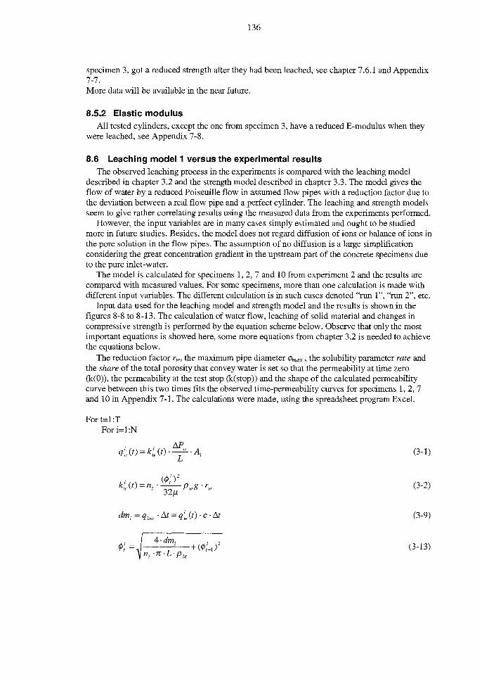
136
specimen 3, got a reduced strength after they had been leached, see chapter 7.6.1 and Appendix 7-7. More data will be available in the near future.
8.5.2 Elastic modulus All tested cylinders, except the one from specimen 3, have a reduced E-modulus when they
were leached, see Appendix 7-8.
8.6 Leaching model 1 versus the experimental results The observed leaching process in the experiments is compared with the leaching model
described in chapter 3.2 and the strength model described in chapter 3.3. The model gives the flow of water by a reduced Poiseuille flow in assumed flow pipes with a reduction factor due to the deviation between a real flow pipe and a perfect cylinder. The leaching and strength models seem to give rather correlating results using the measured data from the experiments performed.
However, the input variables are in many cases simplyestimated and ought to be studied more in future studies. Besides, the model does not regard diffusion of ions or balance of ions in the pore solution in the flow pipes. The assumption of no diffusion is a large simplification considering the great concentration gradient in the upstream part of the concrete specimens due to the pure inlet-water.
The model is calculated for specimens 1,2, 7 and 10 from experiment 2 and the results are compared with measured values. For some specimens, more than one calculation is made with different input variables. The different calculation is in such cases denoted ''ron l", "run 2", etc.
Input data used for the leaching model and strength model and the results is shown in the figures 8-8 to 8-13. The calculation ofwater flow, leaching of solid material and changes in compressive strength is performed by the equation scheme be10w. Observe that only the most important equations is showed here, some more equations from chapter 3.2 is needed to achieve the equations below.
The reduction factor rw, the maximum pipe diameter cf>max , the solubility parameter rate and the share of the total porosity that convey water is set so that the permeability at time zero (k(0)), the permeability at the test stop (k(stop)) and the shape of the calculated permeability curve between this two times fits the observed time-permeability curves for specimens 1,2,7 and 10 in Appendix 7-1. The calculations were made, using the spreadsheet program Excel.
Fort=l:T Fori=l:N
.. M q~ (t) = k:. (t) . __ w. A;
L (3-1)
(3-2)
(3-9)
(3-13)

137
Next i
g(fcc) = jpc· a· (w/c )b
Next t
Where t T i N
Time step (hour) Total calculation time (hour) Ca1culation for pipe size i Number or different pipe sizes (nos.)
See chapter 3 for explanation of the notations used in the equations and in the figures.
Specimen 1, experiment 2:
(3-14)
(3-20)
Two different calculation mns was performed for specimen 1, mn 1 (figure 8-9) and mn 2 (figure 8-10).
In mn 1, the input variables rate, share, rw, and I/>max was set to 1.5,0.4, 104 and 257 /lm respectively. The received permeability from this mn 1 was in good correlation with the measured permeability. The initial value was calculated to 4.7·10'11 mls against the measured 8·10'11 mls and the value at 2000 hours was calculated to 1.5·10'8 mls against the measured 1.6·10'8 mls. The permeability between these two times was ab out the same. The measured curve is however steeper at the time when the permeability accelerated.
In mn 2, the input variables rate, share, rw, and I/>max was set to 1.5,0.0004, 10'3 and 91 /lID respectively. The received permeability from this mn 2 was also in good correlation with the measured permeability, except the initial value. The initial value was ca1culated to 7·10'14 mls against the measured 8·10'11 mls and the value at 2000 hours was ca1culated to 1.2·10'8 mls against the measured 1.6·10'8 mls. The permeability between these two times correlated better than for mn 1 with a steeper acceleration.
In mn 1 the flow pipes are coarser (<Pmax=257 /lm) and alarger share of the pipes lead water (share =0.4) compared to run 2 where <Pmax was 91/lm and the share was 0.004. On the other hand, water is assumed not to flow so easy through the specimen in mn l, the reduction due to tortuous pipes rw is rw=lO,4 compared with 10'3 for mn 2. So, the more and larger but less permeable flow pipes in mn 1 cause almost the same evolution of water flow during time as the fewer and smaller, but more permeable flow pipes in mn 2. The permeability curves in both mn follows the measured flow of water quite good. Run 2 however, gives a much lower initial permeability and also a more rapid increase in water-flow. By setting the fictitious strengthjo to 340 Mpa, the initial values of the compressive strength fit to the measured value for both runs. At the stop time 2060 h for the test, the strength is too low (29 MPa) in mn 1 and too high (46 MPa) in mn 2 compared to the measured values (36 MPa). All input and output data are shown in the figures.

138
,....----..,----....,...---......,-----,...-1-----,-50 --Calculated permeability
.... Measured permeability 45
---Calculated strength
40
1,5E-oa +---'===;==d....--+-----+~~.--tdi._--l
5,OE-09
35 Input data model1 :
dPw=SO m, l..=O.OS m, p,.--2300 kg/m3
30 50=0.7, rate=1.S, rw=10", <l>max=2S7 (!lm),
r---1.-----1l-___ +-__ ----.~~---+ share=0,4 2S '0=300 MPa, K=2.S, a=1.2, b=O.S
20 Output data: model1
15 k(O)= 4.7*10.11 m/s
k(20S0)= 1.S*10" m/s 10
100(0)= 4S MPa 5 Icc(20S0)= 29 MPa
measured S*10·11 m1s
1.S*10" m/s
4SMPa 3SMPa
1,0E-ll .1IIIII1IIIII •• iIIII •••• atlllllll~IIIIId!L-+----_t o 500 1000 1500 2000 2500
Figure 8-9 Specimen 1, expo 2; Late-dried wie 0.8. A comparison of penneability and strength between model 1 and measured values. See chapter 3 for explanation of used notations.
5,OE-09
,...----..,...----....,...----,.----,-t-----,-50 --Calculated permeability
.... Measured permeability 45
---Calculated strength
40
35 Input data model 1:
dPw=SO m, l..=O.05 m, PM=2300 kg/m3
30 50=0.7, rate=1.S, rw=10", <l>max=91 (!lm),
r-----'------1l----+----..ijik---\-!. share=O,0004 2S '0=300 MPa, K=2.S, a=1.2, b=O.S
20 Output data: modell
15 k(O)= 7.0*10.14 mls
k(20S0)= 1.2*10" mls
10 foo(O)= 46 MPa
5 fcc(20S0)= 4S MPa
measured S*10-11m1s
1.6*10'· mls
46MPa 3SMPa
1,0E-ll .1IIIII1IIIII1IIIII.1IItI1IIIII1IIIII •• IIII!IIIIII"'IIIIId!~-l----_t o 500 1000 1500 2000 2500
Figure 8-10 Specimen 1, expo 2; Late-dried w/c 0.8. A comparison of penneability and strength between modell and measured values. See chapter 3 for explanation of used notations.
Specimen 2, experiment 2: Two different calculations were perfonned for specimen 2, run1 (figure 8~ 11) and run2
(figure 8-12). In run1, the flow pipes were supposed to be almost as coarse (<!>m.,.) as for run lfor

139
the late-dried specimen 1 and the share of the flow pipes that can lead water is also the same. The difference is that the reduction parameter r w is set much smaller, so the calculated permeability became the 100 times smaller permeability that was observed in the experiment. The time evolution of the water-flow follows the measured rather weIl in fUll 1. hl run 2, the share of water flow in the flow pipes in relation to the total flow is decreased to 0.04 and the reduction due to deviation between a real pore and a perfect cylinder rw is increased to 10-5. The initial permeability kCO), is the same as in runl, hut the time evolution is not the same and does not at all follow the measured curve.
I,OE-12
B,OE-13
45
~--------~--------+~
---- Calculated permeability
....... Measured permeability
--..-. Calculated strength
35 Input data modell:
~ dPw=60 m, L=0.05 m. PM=2300 kg/m'
:; 6,OE-13 +-----::-------\----------+---------+----------t 30 8 0=0.7, rate=I.5, rr1 O"', $m~=219 (~m),
.i:' share=O,4 ~ 25 , 0 =300 MPa, K=2.5, a=1.2, b=0.5
~ 4,OE-13 J~~~:~~::~~~ 20 Output data: Cii II.
model1 ,..,. ... ....,~ ...... v... ................ if.InI .... ,..,.,..,.**! 15 k(O)= 3.5*10-13 m/s
k(2060)= 4.2*10.13 mls
2,OE-13 +--+------H----------+---------+----------t 10 1,,(0)= 15 MPa
5 Icc(2060)= 16 MPa
O,OE+OO +----------1----------1----------+----------+ O 5000 10000 15000 20000
Tid
measured 4*10·'3m/s
4*10-13 m/s
MPa - MPa
Figure 8-11 Specimen 2, exp, 2; Virgin w/c 0,8. A comparison of permeability and strength between modell and measured values. See chapter 3 for explanation of used notations.

140
----Calculated permeability
45 --Measured permeability
--Calculated strength S,OE-13 +-------1--01--------1 40
35 Inpul data modell:
.te
.§. 6,OE-13 +----,---JL--I-------j dPw=60 m, l=O.OS m, PM=2300 kg/m3
30 So=0.7, rate=I.5, rw=10-5, $max=219 (Ilm), share=0,04
... ~ ~
25 , 0 =300 MPa, K=2.S, a=1.2, b=O.S
E 4,OE-13 ,-"ThW++--1h...--P-"'H'-----=-t 20 Output data: iii
Do modell
,.,.,.,.,....'*'I!I/H,....,.,.,.,..-.j.j ............................. 15 k(O)= 3.5*10-13 m/s
2,OE-13 +--"4----+1-----+----+-----+ 10
O,OE+OO +------1------1------1-------1-O 5000 10000
Tid
15000 20000
k(2060)= 4.2*10-13 m/s
1,,(0)= 15 MPa Icc(2060)= 16 MPa
measured 4*1 O-13m/s
4*10-13 m/s
MPa MPa
Figure 8-12 Specimen 2, expo 2; Virgin w/c 0.8. A comparison ofpermeability and strength between model 1 and measured values. See chapter 3 for explanation of used notations.
Specimen 7, experiment 2: For late-drled wie 1.3 specimen 7 in figure 8-13, the flow pipes (<!>max) are rather coarse and there are also many pipes that can percolate water; i.e. the share of water flow in pipes is high. This leads to a good fitting to the measured permeability curve. The exponent K in the strength relation in equation (3-16) is changed to 1.9 to have a good fitting to the measured initial strength.

141
3,OE-0~r-~"'~:-:I-I-I-I--rr1
_ 2,5E-OS +---f---+----1f--'I""III..-+---+-_.---l
20
-+-Calculated permeability
....... Measured permeability
--Calculated strength
Input data modell: ~ .§. ~ 2,OE-OS
dPw=60 m, 1.=0.05 m PM=2300 kg/ms
H---t--rl-<IIII---I 15 50=0.7, rate=O.S, rw=10", <l>max=355 (!lm), share=O,S ~ '0=300 MPa, K=1.9, a=1.2, b=0.5
~ l,5E-OS
E ~
10 Output data:
l,OE-OS
5,OE-09 +---f---+----1f--+--+----::iI~-_+-T---l
l,OE-ll ~_ .... --.. !I!!e~:r=-_l.-.J--l o 100 200 300 400 500 600 700 800
Tid
k(O)= k(720)=
fcc(O)= fcc(720)=
modell measured 1.S*10·'o mls 2.4*10·'Omts
3.2*10"m!s 3.0*10" mls
21 MPa 18MPa 3MPa 12MPa
Figure 8-13 Specimen 7, expo 2; Late-dried wlc 1.3. A camparison of penneability and strength between modell and measured values. Input data due to table 4, modeIla. See chapter 3 for explanatian of used notations.
Specimen 10, experiment 2: For virgin wlc 1.3 specimen 10 in figure 8-14, the assumed size of the flow pipes is assumed to be the same (<Pmax) as for the late-dried variant of wlc 1.3 (specimen 7). In the calculations of specimens 1 and 2 (w/c 0.8) that is showed above, the selected value of <Pmax was a little lower for the virgin than for the late-dried variant, but here it is the same (<I>max=355Ilm). There is a somewhat smaller selected share of the pipes that can lead water in specimen 10 (share=0.4) than in specimen 7 (share=0.8) and the pipes are selected approximately the same penneable (rw) for specimen 10 and specimen 7. This leads to a good fitting to the measured penneability curve. The exponent K in equation (3-15) is 1.9, as for specimen 7, to have a good fitting to the measured initial strength.

142
8,oE-0,AC:l~~~$~~...,L---J-~--lJ--t.-j 20
-+- Calculated permeability
....... Measured permeability
.......... Calculated strength
r.ln~p~m-'d~am-m~od~e~ll~:-------~
~ dPw=60 m, 1.=0.05 m, PM=2300 kg/m"
S 60E-09 80=0.7, rate=0.5, rw=4*10", <J>mox=355 (11m), .lI:' +---t---j--+--f---+--+--+-,.--H'l---j--+ 1 share=O,4
~ f o=300 MPa, K=I.9, a=I.2, b=0.5
~ E 4,OE-09 Output data:
modell
~ k(O)= 3.6*10'" mls k(1700)= 10*10" mls
2,OE-09 I+--+---t---j~>-t+--;-+--+ s 1,,(0)= 21 MPa fcc(1700)= 6 MPa
1,0E-ll o O 200 400 600 800 1000 1200 1400 1600 1800 2000
Tid
measured 3*10'"m1s 8*10'· mls
21 MPa 18MPa
Figure 8-14 Specimen 10, expo 2; Virgin w/c 1.3. A comparison ofpermeability and strength between modell and measured values. See chapter 3 for explanation of used notations.
Conclusion Leaching modell described in chapter 3.2 and the strength model in chapter 3.3 have a
simple and physically reasonable basis. The parameters used C, W, Vair, dPw, L and Co are determined by the experiment while the parameters if>m= share, rw, and rate are seleeted to fit the experimental results of permeability. With these input parameters, the model and the experimental data corresponds very weIl with each other.
The chose of variables must however be discussed more before it can be said to be a good model. So far input data concerning the flow pipe size and the share of water flowing in these pipes are selected so that a good correlation with experiments is obtained. In a good model, the data should be based on observations.
A weak point of the model is that it only considers flow of Ca-ions due to convection (by the water flow). Diffusion must be regarded where there are large concentration gradients and when the concrete is of high quality with small flow pipes. Besides, the mass balance between different ions in the pore solution is not regarded in modell. This is of minor importance for high permeable specimens with many, coarse flow pipes, because Ca(OH)2 almost directly after start of the test becomes the main dissolved compound. The other compounds in cement paste have either aIready leached out due to their high solubility and small initial content (KOH and NaOH), or they have a low solubility.
8.7 DIssolutlon of Ca(OH)2 In purewater As can be seen in figure 8-15, the measured dissolving process was very rapid at the
beginning. The measured dis solution should have been even more rapid if the solution had been stirred from the beginning. Now, stirring started after 240 seconds.

143
The dissolving reaction is also calculated (figure 8-14) by the calculation scheme "model Guntelberg" in chapter 2.2.1 and with the method in chapter 3.5, which describes a dissolving reaction.
Calculation simulates the dis solution in cavities between particles. The following data were used in the model; the particle diameter if> is 2·10-4 m, the diffusion coefficient in the pore solution in the cavities kioll(aq) is lO-lO m2/s, the diffusion layer in each solid particle tes) is 10-9 m and the diffusion coefficient in the diffusion layer in the solid particle to kion(s) is 10-11 m2/s. The variables used are assumed, but quite reasonable.
The calculation gives surprisingly good agreements with the measured values (figure 8-14). One calculation used the solubility product Ksp = 4.10-6 and the other calculation used Ksp = 6·10-6. The one with Ksp = 4.10-6 fitted the measured dis solution curve before the stirring and the other with Ksp = 6.10-6 seems to fit a measured curve if it had been stirred from the start. The stirring made of course the solubility increase.
Due to Atkins & Jones (1997) and Aylward & Findlay (1994), the Ksp should be about 6.10-6,
so the used values of Ksp seems reasonable.
0,7
~ -; 0,6 o 5 ~ 0,5 .5 ftS ~
... ' CJ 04 ;g Me o 1/1
§ 0,3 ~S\Z :...-
"tI 'iii .= 0,2 o c ~ 0,1 o
CJ
o o
,~ i.ialculat d
f 50 100
.~
150 200 250
Time (s)
I I I ! i i ! L-f-II- I
I
300 350
! ....... Measured Ca(aq) gli
-+-Calculated Ksp=4*
....... Calculated Ksp=6*
I I I
1QA-6 g/I
10"-6 g/I
400 450 500
Figure 8-15 Measured and calculated dissolving of Ca(OH)2(s) in pure water.
8.8 Conclusions
8.8.1 Experiments The purpose of this work was to study the flow of de-ionised water under pressure through
homogenous concrete of different qualities and curing history and the leaching effect of this waterflow.
The laboratory test was accelerated regarding (i) the pressure gradient which is about 100 times higher than in a real structure, (ii) the water to cement ratio which is not below 0.80 although the normal value in structures is 0.55 to 0.60, and (iii) the water aggressiveness; deionized. On the other hand, the test was retarded since there were no aggressive ions in the water (C02, W, sol-, etc) and the temperature was constant at 20°C.

144
The experimental results show that percolating pure water through concrete specimens have an ability to dissolve hydration products, probably mainly Ca(OHh and also to carry the dissolved ions out of the specimen by diffusion or convection.
Depending on the wie ratio and the curing history, the permeability was different. A high hydration ratio made the specimens more porous with higher water permeability.
Virgin specimens had a low and constant permeability with small deviations between the specimens. However, one w/c 0.8 and one w/c 1.3 had a rapidly increased permeability after some time. Probably the same will happen with the other specimens after longer time of leaching.
Late-dried specimens, became 100 times more permeable than in the virgin state. This was probably caused by micro-cracks during the drying. Because of the high hydration ratio almost all cement had been consumed and there was not much cement left for any self-healing. These specimens had often a rapidly increased permeability after some time.
Early-heated specimens, had a about 100 times higher initial water permeability than in the virgin state. Then, the permeability rapidly decreased due to a restarted hydration and a resulting self-healing to near the same value as in the virgin state. Probably these specimens will also reach the point where the permeability rapidly increase. It is only a matter of time.
In the high-permeable eonerete, the water seems to have flowed in a rather few, distinct flow pipes. In these pipes, the water had dissolved solids, probably mainly Ca(OH)2) and the pipes grew wider. Then, the water flow increased further and even more solid material was leached. Finally, the pipe walls became so exhausted in lime so that the leaching rate and the water flow increased only slowly. The dissolution of the pipe walls was a diffusion process from the interior of the solid and towards the pipe wall. Around these pipes the concrete became very disintegrated with almost no continuos cementitious materialleft to maintain strength and tightness.
Between the flow pipes, or in less permeable concrete, more of the leaching seemed to be govemed by diffusion to the inlet water at the upstream end.
A detailed analysis of one specimen, showed that most calcium was leached from the upstream part of the specimen. This was probably due to diffusion in the upstream direction. Another possibility is that the permeating water became saturated with lime already at the upstream part due to dis solution of lime there. Therefore, its dissolving ability was very much reduced when it reached the deeper parts of the specimen. Another part of the specimen, which lost quite lot calcium, was where the aggregate content was high. The cause of the leaching in this part was probably due to water percolation in porous and easily soluble areas. Because of leaching, the porosity was increased in these parts of the specimen.
The measured residual content of substances in the leached specimens corresponded fairly well to the measured ionic flow in the drainage water flow.
The results also show that when solid material is leached, the porosity will increase and the strength will decrease due to less load-bearing solids. The strength reduction due to leaching, was to a high degree a local phenomenon. In parts of the specimen, where much solid material had been leached, the strength was very much reduced. But if these parts were small compared to the whole specimen, the average strength of the whole specimen was not much influenced. The number of specimens used for strength testing were however too few for any more detailed analysis.
8.8.2 Modelling The leaching modell is very simple, but despite this, it gave interesting results. This model
imitates leaching by assuming that there are a certain number of flow pipes in the eonerete. The flow ofwater was assessed by a "reduced" Hagen-Poiseuille law.

145
However, the pipes were modelled with only one element through the whole body and because of this, no gradients of the leaching effects could be predicted. Another weak point in the model is that no diffusion in the upstream direction is regarded. The experiment shows that diffusion upstream to the pure water at the inlet was strong. Also, the dissolving reaction term was modelled in a very simplified manner. The model is simply calculated using an Excel file. It can easily be connected to ordinary static calculations for estimations of the safety marginal for a concrete dam during time.
8.8.3 Future research The following additional research ought to be made:
./ A more precise study of the diffusion of ions upstream in addition to the study performed in this work of the convection of ions downstream .
./ Future experiments should regard leaching in cracks or larger flow pipes. These can be artificially be produced in the concrete specimens before the leaching test starts .
./ ESEM and MIP studies from the leached cracks or flow pipes should be used for investigating chemical and physical changes of the structure .
./ A comprehensive study of the strength of leached specimens .
./ Development of more sophisticated models that take consideration to the more complicated features in the leaching process. For example, the balance of mass (equation 2-2) can be formulated and solved by the Finite Element Method. This requires development of the individual terms in the equation and also verification by experiments.
146
References
Adenot, F., Richet, C. (1997), Modelling of the chemical degradation of a cement paste, Mechanisms of chemical degradation of cement based systems, E & FN Spon, London.
Alemo, J., Johansson, N., Bronner, N. (1988), Dissolution of cement grout by flowing water, Vattenfall Utveckling och Miljö, 1988, Råcksta, Vällingby.
Atkins, P., Jones, L. (1997), Chemistry Molecules, Matter, and Change, 3rd edition, W. H. Freeman and Company, New York.
Aylward, G., Findlay, T. (1994), S I Chemical Data (SICD), John Wiley & Son, 3rd edition.
Ayora, C. et al (1998), Weathering ofiron sulfides and concrete alteration: Thermodynamic model and observation in dams from central Pyrenees, Spain, Cem. & Coner. Res. Vol. 28, no. 9, pp 1223-1235.
Bal'shin (1949), Relation ofmechanical properties ofpowder metals and their porosity and the ultimate properties ofporous metal-ceramic materials, Dokl. Akad. Nauk. SSSR, 67, 5.
Beckman O., Kjöllerström B., Sundström T. (1986), Basic thermodynamicsfor college studies, (in Swedish), Almqvist & Wiksell, Sweden.
Bentz, D. P., Garboczi, E. J. (l991a) A digitized simulation modelfor microstructureal development, Advances in Cementitious Materials, Ceramic Transactions Vol. 16, pp. 211-226.
Bentz, D. P., Garboczi, E.J. (1991b) Percolation ofphases in a three-dimensional cement paste microstructural model, Cement and Concrete Research, Vol. 21, pp. 325-344.
Bentz, D. P., Garboczi, E. J. (1992), Modelling the leaching ofcaldum hydroxidefrom cement paste: effects on pore space percolation and difJusivity, Materials and Structures, Vol. 25, 523-533.
Bentz, D. P. (1999), Modelling cement microstructure: Pixels, particles, and property prediction, Materials and Structures, Vol. 32,187-195.
Bemer, U. R. (1988), Modelling the incongruent dissolution ofhydrated cement minerals, Radiochimica Acta, 44/45, pp. 387-393.
BBK 94, Concrete structures, (in Swedish), Boverket 1994.
BTG M, The concrete Handbook Material ed. 2, (in Swedish), Svensk Byggtjänst, Stockholm 1994.
Carde, C., Francois, R. (1997), Aging damage model of concrete behavior during the leaching process, Materials and Structures Vol. 30, pp 465-472.

147
Carde, C., Francois, R. (1997), "Effect ofITZ leaching on durability of cement-based materials", Cement and Concrete Research, Vol. 27, pp 971-978.
Carde, C., Francois, R, Torrenti, J-M. (1996), Leaching ofboth calcium hydroxide and C-S-H from cement paste: Modelling the mechanical behaviour, Cement and Concrete research, Vol. 26, No. 8, pp. 1257-1268.
Carde, C., Francois, R., Ollivier, J-P. (1995), Microstructural changes and mechanical effects due to the leaching of calcium hydroxide from cement paste. Proceedings of the Materials Research Society' s Symposium on Mechanisms of Chemical Degradation of Cement-based Systems, Boston, 27-30.
Carde, C., Francois, R, Ollivier, J-P (1997), Microstructural changes and mechanical effects due to the leaching of calcium hydroxide from cement paste. Mechanisms of chemical degradation of cement based systems, E & FN Spon 1997, London.
Carde, c., Francois, R (1997), "Effect of the leaching of calcium hydroxide from cement paste on mechanical and physical properties", Cement and Concrete Research, Vol. 27, pp 539-550.
Cederwall, K. (1979), Hydraulicsfor civil engineers, (in Swedish), Liber läromedel, Malmö.
Constantiner, D., Diamond, S. (1995), Pore solution analysis: Are there pressure effects?, Proceedings of the Materials Research Society' s Symposium on Mechanisms of Chemical Degradation ofCement-based Systems, Boston, 27-30.
Davis R E. (1950), "Permeability and Triaxial Tests of Lean Mass Concrete", Corps of Engineer.
Delagrave, A., Gerard, B., Marchand, J. (1997), Modelling the calcium leaching mechanisms in hydrated cement pastes, Mechanisms of chemical degradation of cement based systems, E & FN Spon, London.
Duchesne, J., Reardon, E. J. (1995), Measurement and prediction ofportlandite solubility in alkali solutions, Cement & Concrete Research, vol. 25, no. 5, pp 1043-1053.
Edvardsen, C. (1996), Water permeability and autogenous healing of cracks in concrete, (in German), Heft 455, Deutscher Ausschuss fUr Stahlbeton, Berlin.
Ekström, T. (2000), Leaching of concrete Experiments and Modelling, Licentiate thesis report TVBM -7153, Div. of Building Materials, Lund Institute of Technology.
Engkvist, 1., Albinsson, Y., Johansson Engkvist, W. (1996), The long term stability of cementLeaching tests, SKB technical report 96-09, KTH, Göteborg.
Eriksen, K., Coresfrom the Storfinnforsen dam, (in Danish), Statens Vejlaboratorium, Roskilde, Denmark.

148
Fagerlund, G. (1980), Moisture-mechanical properties, (in Swedish), The concrete Handbook Material, Svensk Byggtjänst, Stockholm.
Fagerlund, G. (1987), Relations between the strength and the degree of hydration or porosity of cement paste, cement mortar and concrete, Seminar on Hydration of Cement, Aalborg Portland, Aalborg.
Fagerlund, G. (1989), Concretefor hydraulic structures, (in Swedish), CEMENTA, Danderyd.
Fagerlund, G. (1991), Freeze testing of concrete from the Stoifinnforsen dam, (in Swedish), Div. of Building Materials, Lund Institute of Technology.
Fagerlund, G. (1994), Structure and development of structure, (in Swedish), The concrete Handbook Material, Svensk Byggtjänst, Stockholm.
Fagerlund G. (1996), Service life prediction of concrete structures, (in Swedish), report TVBM-3070, Lund.
Fagerlund, G. (1997), Deterioration, service life and repair of concrete structures-knowledge and research needs, Div. of Building Materials, Lund Institute of Technology.
Fagerlund, G. (1997a), Composite models and compositefonnulas, (in Swedish), Compendium in Building Material Div. of Building Materials, Lund Institute of Technology.
Fagerlund, G. (1997b), The chemistry of cement based binder, (in Swedish), Compendium in Building Material Div. of Building Materials, Lund Institute of Technology.
Fagerlund, G. (1997c), Temperature development in concrete, (in Swedish), Compendium in Building Material Div. of Building Materials, Lund Institute of Technology.
Fagerlund, G. (2000), Leaching of concrete, contribution to EU-project CONTECVET, Div. of Building Materials, Lund Institute of Technology.
Faucon, P., Bonville, P., Adenot, F., Genand-Riondet, N., Jacquionot, J., Virlet, J. (1997), 57Fe Mässbauer study of cement water degradation, Advances in Cement Research, 9, No 35, pp. 99-104.
Faucon, P., Gerard, B., Jacquinot, J., Marchand, J. (1996), Leaching of cement: study of the suiface layer, Cement and Concrete Research, vol. 26, no. 11, pp 1707-1715.
Faucon, P., Adenot, F., Jacquionot, J., Petit, J., Cabrillac, R, Jordan, M. (1998), Long-tenn behaviour of cement pastes used for nuclear waste disposal: Review of physico-chemical mechanisms of water degradation, Cement & Concrete Research, vol. 28, No.6, pp. 847-857.
Freeze, R. A, Cherry, J. A (unknown), Groundwater, Dep. Of Geological Sciences, Univ. Of British Columbia, Vancouver.

149
Garboczi, E. J., Bentz, D.P. (1992), Computer simulation of the diffusivity of cement-based materials, J. Mater. Sci. 27.
Garbotczi, E. J., Bentz, D. P. (1996), Multi-Scale Picture of concrete and its transport properties: Introduction for non-cement researchers, NISTIR 5900, Gaitersburg, U.S.A.
Garboczi, E. J., Bentz, D.P. (1998), Modelling AnalyticallNumerical theory of the diffusivity of concrete, Advances in Cement Based Materials 1998;8:77-88.
Granholm, H., Werner, D., Giertz-Hedström, S. (1934), Investigation of the suitability of concrete pipes for road drainage, (in Swedish), Betong, 1934(19):1, p.1-84.
Grattan-Bellew, P. E. (1996), Microstructural investigation of deteriorated Portland cement concretes, Construction and Building Materials, Vol. 10, No. 1, pp. 3-16.
Grube, H. and Rechenberg, W. (1989), Durability of concrete structures in acidic water, Cement and Concrete Research, Vol. 19, pp. 783-792.
Halvorsen, U. (1966), Corrosion of steel and leaching of lime near cracks in concrete structures, (in Swedish), Bulletin 1, Div. of Building Technology, Lund Institute of Technology.
Hearn, N., Detwiler, R. J., Sframeli, C. (1994), Water permeability and microstructure ofthree old concretes, Cement and Concrete Research, Vol. 24, No. 4, pp. 633-640.
Hedenblad, G. (1993), Moisture Permeability of Mature Concrete, Cement Mortar and Cement Paste, report TVBM-1014, Div. of Building Materials, Lund Institute of Technology.
Hedin, R. (1962), Processes of Diffusion, Solution and Crystallistation in System Ca(OHhH20, Swedish Cement and Concrete Research Institute, Stockholm.
ICOLD (unknown), Deterioration of dams and reservoirs, examples and their analysis, Paris, France.
Imhof-Zeitler, C. (1996), Flief3verhalten von Fliissigheiten in durchgehend gerissenen Betonkonstruktionen, (in German), Heft 460, Deutscher Ausschuss fUr Stahlbeton, Berlin.
Janz, M. (1997), Methods ofmeasuring the moisture diffusivity at high moisture leveis, Report TVBM 3076, Div. of Building Materials, Lund Institute of Technology.
Janz, M., Retention curve and pore size distribution measured with pressure plate and pressure membrane extractiors, Methods a nd calibration, Report TVBM-9050, Div. of Building Materials, Lund Institute of Technology.
Jennings, H.M. (1986), Aqueous solubility relationships for two types of Calcium silicate hydrates, Journal ofthe Ceramic Society, 69, pp. 614-618.

150
Johannesson, B. (1998), Modelling of transport processes involved in service life prediction of concrete; important principles, Licentiate thesis report TVBM - 3083, Div. of Building Materials, Lund Institute of Technology.
Koenders, E. (1997), Simulation ofVolume Changes in Hardening Cement-Based Materials. Delft University Press, Netherlands.
Kriz, D. (1991), Laboratory product handbook, Chemel analys AB, Lund.
Lagerblad, B., Trägårdh, J. (1994), Conceptual modelfor concrete long time degradation in a deep nuclear waste repository, SKB Technical report 95-21, Swedish Cement and Concrete Research Institute, Stockholm.
Lawrence, C. D. (1982), Permeability measurements on concrete, Cement and Concrete Association.
Lea, F. M. (1983), The chemistry of cement arid concrete, third edition, Edward Arnold (publishers ) Ltd, London.
Marchand, J., Sarnson, E., Maltais, Y. (1999), Modelting ionic diffusion mechanisms in saturated cement based materials - an overview, CRlB-Department of civil engineering, Laval Univ., Quebec, GIP4r7.
Mary, M. (1936), contribution to the discussion with Ruettgers, Proceedings of the ACI, vol. 32, pp.125-129.
Mason P.J. (1990), The effects of aggressive water on dam concrete, Water Power & Dam construction.
Melander, R. (1997), Betongdammars kondition och beständighet, Licentiate Thesis, Div. of Hydraulic Engineering, Royal Institute of Technology, Stockholm.
Meyers, S. L. (1936), contribution to the discussion with Ruettgers, Proceedings of the ACI, vol. 32, pp. 230-233.
Moskvin, V. (1980), Concrete and reinforced concrete deterioration and protection, Mir Publishers, Moscow.
Möller, G., Petersons, N. (1994), Strength, (in Swedish), The concrete Handbook Material, Svensk Byggtjänst, Stockholm.
The Swedish National Encyclopaedia, (1989-2000) Sweden.
Nilsson, L.-O. (1994), Moisture and Concrete, (in Swedish), The concrete Handbook Material, Svensk Byggtjänst, Stockholm.
Nyame, B. K., Illston, J. M. (1981), "Relationships between permeability and pore structure of hardened cement paste", Magazine of Concrete Research, Vol. 33, No. 116.

151
Ottosen, N., Petersson, H. (1992), Introduction to Finite Element Method, Prentice Hall Europe.
Pitzer, K. S. (1991), Activity coefficients in electrolyte solutions, p. 75, CRC Press, Boca Raton, FL.
Powers, T. C. (1962), Physical properties of cement paste, From: Chemistry of cement. Proceedings of the 4th International Symposium, Washington, 1960. Washington D.C., 1962. National Bureau of Standards, Monograph 43, vol. II, pp. 577-613, 1962.
Powers T. C. (1958), The physical structure and engineering properties of concrete. PCA Research & Development Laboratories, Bulletin 90, Chicago.
Persson, B. (1992), "Högpresterande betongs hydratation, struktur och hållfasthet", Report TVBM-1009, Div. of Building Materials, Lund Institute of Technology.
Roehling, S. and Nietner, M., A model to describe the kinetics of structure formation and strength development, VTT Symp. 115, ed. Heikki Kukko, 1990 Microstruct. Prop. Concr., 1990, pp.5-51.
Roy, D. M. and Jiang, W. (1995), Concrete chemical degradation: Ancient analogues and modem evaluation, Proceedings of the Materials Research Society' s Symposium on Mechanisms of Chemical Degradation of Cement-based Systems, Boston, USA, 27-30.
Ruettgers, A. (1936), final reply in discussion, Proceedings of the ACI, vol. 32, pp. 337-389.
Ruettgers, A., Vidal, E. N., Wing, S. P. (1935), An investigation of the permeability ofmass concrete with particular reference to Boulder Dam, ACI Journal, Proceedings 1935(31):4, pp. 382-416.
Ryshkewitch, T. (1953), Compression strength ofporous sintered alumina and zirconia. Journal of the American Ceramic Society, vol. 36.
Scheidegger, A. E., (1963) The physics offlow through porous media, University of Toronto Press
Seidell, A. (1965), Solubilities ofinorganic and metal-organic compounds, Princeton.
Seveque, J., Cayeux, M., Elert, M., Nouguier, H. (1992), Mathematical modelling ofredioactive waste leaching, Cement and Concrete Research. Vol. 22, pp477-488.
Stronach, S. A., Glasser, F. P. (1997), Modelling the impact of abundant geochemical components on phase stability and solubility of the CaO-Si02-H20 system at 25°C: Na+, r, SO/-, cr and col-, Advances in Cement Research, vol. 9, No. 36, pp. 167-181.
Stumm W., Morgan J. J. (1996), Aquatic chemistry, John Wiley & Sons, Inc., U.S.A.

152
Sällström, S. (1964), Investigation of the durability of porous cement mortar exposed to continuing water percolation, (in Swedish), Statens Vattenfallsverk, Preliminary report, Stockholm.
Sällström, S. (1991), The Storfinnforsen dam; investigation of the status and repair demand of the concrete, (in Swedish).
Takemoto, K, Takahashi, H., Takagi, S. (1959), Leaching of lime from various kinds of cement mortar and its effect on the strength, Japan Cement Engineering Ass., Review of the 13th
Cement Meeting, Tokyo.
Terzaghi, R. D. (1948), Concrete deterioration in a shipway, Proceedings of the ACI, vol. 44, pp. 977-1005.
Terzaghi, R. D., answer to K Mather regarding the paper "Leaching of lime from concrete, ACI February 1950, pp. 475-477.
Thaulow, T. and Jakobsen, U. H. (1995), The diagnosis of chemical deterioration of concrete by optical microscopy , Proceedings of the Materials Research Society' s Symposium on Mechanisms of Chemical Degradation of Cement-based Systems, Boston, 27-30.
Taylor H. F. W. (1990), "Cement chemistry", Academic Press, London.
Tremper, B. (1931), The effect of acid waters on concrete, Proceedings of the ACI, vol. 28, pp. 1-32.
Trägårdh, J., Lagerblad, B. (1998), Leaching of90-year old concrete mortar in contact with stagnant water, SKB Technical report TR-98-11, Swedish Cement and Concrete Research Institute, Stockholm.
Unsworth, H. P., Lota, J. S., Hubbard, F. H. (unknown magazine and year), Microstructural and chemical changes during leaching of cementitious materials.
Wallin, M. (1988), Afundamental analysis of the Rate of Limestone Dissolution from a Plane geometry, Licentiate thesis, Department of Chemical Engineer, University of Luud.
Wang, K, Jansen, D., Shah, S. (1997), Permeability ofcracked concrete, Cement and Concrete Research, Vol. 27, No. 3, pp. 381-393.
White, Frank M. (1979), Fluid mechanics, McGraw-Hill.
Winslow, D. N., Diamond S. (1970), A mercury porosimetry study of the evolution ofporosity in portland cement paste. Journal of Material, 1970(5):3, pp. 564-585.
y sberg, G. (1979), Connection between water cement ratiolwater-air-cement ratio and compressive strength, report Ra 3:79, Swedish Cement and Concrete Research Institute, Stockholm.

153
Young J. F. (1985), Hydration ofportland cement, Ed. Roy D. M. Institutional Modulus in Cement Science, Materials Research Laboratory, University Park, Pennsylvania State University, Pennsylvania.
Zamorani et al (1986), Calcium release from cement samples of different size, Cement and Concrete Research, vol. 16, pp 394-398.
Zienkiewicz, O. C., Taylor, R. L., (1989), The Finite Element Method, 4th edition, McGraw-Hill, New York.


AS-l
APPENDIX TO CHAPTER 5
5-1 Test cells 5-2 Evaporation from measuring vessels

.-<
o + o
(1J
ru
. 1,\'lJ/'~-® f{ijJ;{//UJ/'J'YJj
ASSEMBLING .J'2
TOP LID ):2
THREADED HOL E ISO 7/1 118'
DBSERVE DIRECTIDN!
THREADED HDLE ISO 7/1 118'
DBSERVE DIRECTIDN!
bO
l~ ~ I. 45 .1
71
STEEL RING 1:2
BOTTTOM 1:2
FOR D-RING OUTER EDGE STEEL RING + CA 0,2MM
~t~ I. 120 .1
A-A 1:2
7 16
6 4
5 4
4 2
311
2 1
1 1
NO NOS
'vIASHES
NUTS
SCRE'w'S
D-RINGS
STEEL
RING
LID
LID
DESIGNATIDN
LUNDS lNSmUTE DF TECHNDLDGY DEP. DF BU1LDlNG MAT.
IIMlAV,IC*SIm:AADAV
BRB 12x22 FZV
116M HlO FZV
M6S Ml0x110 FZV
[l-RINGS 59,5x3
INSIDE PRESSUREI
552343 ~MNESRöR 71x40, L:060, TURNING
CDNICAL INSJDE, SUlTS FOR D-RINGS
IN BDTH ENDS.
$52343
S52343
MA1ERIAl IREHARK
A 12
LEACH1NG EXPER1MENT 3 TEST CELL
TEM 1981126
TOIUI'Eh'rtrr. I 00106
lI.~Djm-lo-H
lNFRADAMM
~ ~ ~ VI I
.......
~ (l)
'" ..... ()
~
~ &.
I ~ .j::. VI
~
~ N

lA
LID 1:5
+ CA O.~ 1'\1'\
% I (lJ% ~
~1"'1~lru(i" J !2l240 J
A-A 1:5
\
;f I
ASSEMBL1NG OF CELL 1:5
STEEL RIING 3
115 I
"" m. Hm, .j60 ~ 1 j~ ,,~,,: ~
l} !2l1S0 ~ I !2l180 7
/I B-h=< /I
if
Rfl.AlTONSRftNING ~ ~IILAO BYGGN.'ZISLOVSRfTNlNG f'OfiHANDSKOPJA
7 12 WASHES
6 6 NUTS
5 6 SCREWS
4 " D-RINGS
3 l STEEC
RING
2 LID
LID
NO NOS DESIGNATlDN
LUNDS INSTITUTE OF TECHNOLOGY DEP. DF BUILDING MAT.
öi~~1ii T_ .....
ll/I5'l'!/11-ID-14
BRB 13x2:4 FZV
MGM Ml2 FZV
M6S M12xlfO fZV
INSIDE PRESSURE 800 kP!;).
1552343 11IMNESRÖR lBOxl50. L==6D. TURNING
CONICAL INSIDE. SUlTS FOR D-RINGS
IN :BOTH ENDS,
S52343
552343
MATERIAL REHARI<
LEACHING EXPERIMENT 3 TEST CELL
... INFRADAMM
_.+ ... -
~ ~ ~ Ul I ......
~ ~ ('l
~
~ e: i Pl ...... Ul Ul
§
~ I
W

APPENDIX 5-2: Evaporation from the measuring vessels A5-4
In the leaching experiment were rubber plugs and rubber balloons used to stop flow of vapor and air to and from the measuring vessels. A permeability test was performed for these plugs and balloons. The leakage appeared to be negligible, see figure l.
Figure shows that the evaporation was about 200 times less than the smallest measured drainage water flow.
~ S 1,00E-11 c o
~ o ~ 1,00E-12
CP "C e
Evaporation check in measuring vessel byrett and beaker .
...... Min. measured water flow for 25 mi byrett (exp. 2, specimen 2).
__ Min. measured water flow for 0.5 I beaker (exp. 3, specimen 10) .
....... Measured evaporation with byrett 50 mi with on ly rubber balloon
""*"" Measured evaporation with beaker 0.5 I with rubber balloon.
::> 1,00E-13 -j----------------------+--~---------' !R :;:
1 ,00E-14 -j-----,--------,------''In---;L----,-------,---------i o 1000 2000 3000
Time (h)
Figure l Check of evaporation from measuring vessels.
4000 5000 6000

APPENDIX TO CHAPTER 6
6-1 Sieve curves of aggregate and concrete composition 6-2 Overview of casting, curing and leaching tests
A6-1
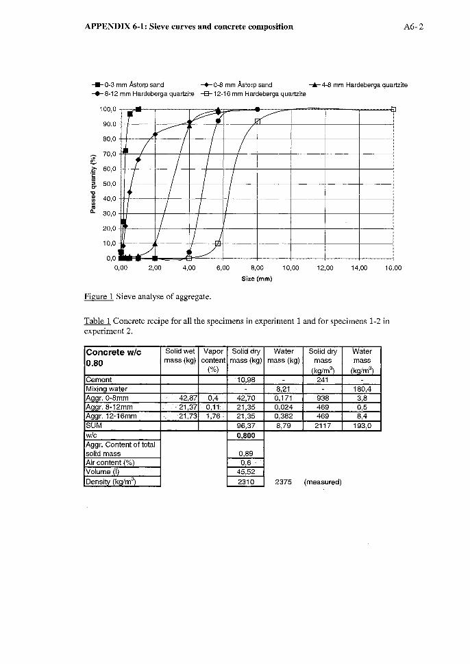
APPENDIX 6-1: Sieve curves and concrete composition A6-2
___ 0-3 mm Åstorp sand -+-0-8 mm Åstorp sand ...... 4-8 mm Hardeberga quartzite ..... 8-12 mm Hardeberga quartzite -8-12-16 mm Hardeberga quartzite
100,0
90,0
80,0
~ 70,0 C ~ 60,0 c III :::J 50,0 CT 'tI ID 40,0 Ul
= o.. 30,0
20,0
10,0
0,0
- ...... ,. V-. tV T
)V / I I I I I / / I
!
f I I / I / I I / l
i
+ / I I I I I I I / I I
/ / J I !~ , ~ I
0,00 2,00 4,00 6,00 8,00
Size (mm)
10,00 12,00 14,00 16,00
Figure 1 Sieve analyse of aggregate.
Table 1 Concrete recipe for all the specimens in experiment 1 and for specimens 1-2 in experiment 2.
Concrete wIe Solidwet Vapor Solid dry Water Solid dry Water
0.80 mass (kg) content mass (kg) mass (kg) mass mass (%) (kg/m3) (kg/m3)
Cement .10,98 - 241 -Mixing water - 8;21 - 180,4 Aggr.0-8mm . ·.····· .. ·42,87 0,4 ' .. 42,70 0,171 938 3,8 Aggr.8-12mm i 2),37 0,11. 21,35 0,024 469 0,5 Aggr.12-16mm <i 21,73 1,76 21,35 0,382 469 8,4 SUM 96,37 8,79 2117 193,0 w/c 0,800 Aggr. Content of total solid mass 0,89 Air content (%) 0,6. '. Volume (I) 45,52 Density (kg/m3) 2310 2375 (measured)

APPENDIX 6-1: Sieve curves aud concrete composition A6- 3
Table 2 Concrete recipe for specimens 3-5 in experiment 2.
Concrete wIe Solid wet Vapor Solid dry Water Solid dry Water
0.80 mass (kg) content mass (kg) mass (kg) mass mass (%) (kg/m3 ) (kg/m3 )
Cement 10,98 - 241 -Mixing water - 8,48 - 186,0 A~gr. 0-8mm 42,89 0,44 42,70 0,189 936 4,1 Aggr. 8-12mm 21,4 0,11 21,38 0,024 469 0,5 Aggr.12-16mm 21,4 0,39 21,32 0,083 467 1,8 SUM 96,37 8,78 2113 192,5 w/c 0,799 Aggr. Content of total solid mass 0,89 Air content (%) 0,8 Volume (I) 45,60 Density (kg/m3) 2306 2370 (measured)
Table 3 Concrete recipe for specimens 6-10 in experiment 2.
Concrete wIe Solid wet Vapor Solid dry Water Solid dry Water
1.30 mass (kg) content mass (kg) mass (kg) mass mass (%) (kg/m3) (kg/m3)
Cement 7,2 - 177 -Mixing water - 9,08 - 223,2 Aggr. 0-8mm 37,4 0,40 37,25 0,150 916 3,7 Aggr.8-12mm 18,7 0,20 18,66 0,037 459 0,9 Aggr.12-16mm 18,7 0,10 18,68 0,019 459 0,5 SUM 81,79 9,29 2010 228,2 w/c 1,290 Aggr. Content of total solid mass 0,91 Air content (%) 0,8 Volume (I) 40,69 Density (kg/m3) 2239 2317 (measured)

APPENDIX 6-1: Sieve curves and concrete composition
Table 4 Concrete recipe for specimens 1,6-7,20-30 in experiment 3.
Concrete wIe Solid wet Vapor Solid dry Water Solid dry Water
0.60 mass (kg) content mass (kg) mass (kg) mass mass (%) (kQ/m3) (kQ/m3)
.9 - 335 -MixinQ water 3,4 .' 126,6 Aggr.0-3mm O 0,0 Aogr. 0-8mm 35 5;5 33,08 1,925 1232 71,7 Aggr.4-8mm ., 15 0;7, .. 14,90 0,105 555 3,9 SUM 56,97 5,43 2122 202,2
w/c 0,603 Aggr. Content of total solid mass 0,84 Air content (%) 1;3 Volume (I) 26,85
Density (kg/m~ 2324
Table 5 Concrete recipe for specimens 8-10, 31-36 in experiment 3.
Concrete wIe Solid wet Vapor Solid dry Water Solid dry Water
0.80 mass (kg) content mass (kg) mass (kg) mass mass (%) (kQ/m3) (kQ/m3)
·9 289 Mixing water .·· .. 5,75 . 184,5 Aggr.0-3mm O 0,0 AQor. 0-8mm .... : ... 38 3~3· 36,75 1,254 1179 40,2 Aggr.4-8mm ... 18 1;1 17,80 0,198 571 6,4 SUM 63,548 7,202 2039 231,0
w/c 0,800 Aggr. Content of total solid mass 0,86 Air content (%) I:, t,3·· Volume (I) 31,17
Density (kg/m3) 2270 2325
The air content was measured by the pressure method in an apparatus of type Bluhm und Feurherdt containing 8.0 litre.
The volume in the tables were calculated as:
V el P~m+(Wm,,+Wagg)1 p.,+(Aggo_.+Agg'_1l +Aggll_1.)I Pagg
l-Air
le. for concrete table 1:
v = 10.98/3.1 + 0.6/1 + 42.7 12.55 + (21.35 + 21.35)/2.64 = 45.5 l 1-0.006
A6-4
The cement content per m3 then become C=10.98/0.0455=241 kglm3 which is used in table 1.
To the right of the calculated density is also one measured given.

APPENDIX 6-2: Overview of castings, curing and leaching tests A6-5
Table 6 Experiment 1. Casting, curing and leaching test.
Specimen W/c Water Water curing Eressing
0.8 83 days 77 days
2 0.8 96 days 64days
3 0.8 96 days 64days
4 0.8 96 days 64days
5 0.8 93 days 61 days
6 0.8 91 days 42days
7 0.8 90 days 41 days
8 0.8 91 days 42 days
9 0.8 92 days 43 days
10 0.8 96 days 44days
Table 8 Experiment 2. Casting, curing and leaching test.
Speci- W/c Water Oven Vacuum Vacuum Leaching test Water pressing men curing +55°C sucldng suclring stop
in water in air 6 bar 3 bar 2 bar 1 bar
Il) 0.8 119 14 days 1 day 1.5 hour 87 days 13 days After 100 days days No No
21) 0.8 127 No No No 497 68 days No No Still running days days2)
3 0.8 201 14 days 1 day 1.5 hour 306 68 days No No After 374 days days days
4 0.8 201 14 days 1 day 1.5 hour 487 68 days No No Still running days days2)
5 0.8 201 No No No 287 68 days No No After 355 days days days
6 1.3 58 days 7 days 1 day 1.5 hour 71 days 2 days 1 day 18 days After 92 days
7 1.3 58 days 7 days 1 day 1.5 hour 71 days 2 days 1 day 15 days After 89 days
8 1.3 58 days 7 days 1 day 1.5 hour 71 days 2days 1 day 18 days After 92 days
9 1.3 58 days No No No No No No No Abounded
10 1.3 75 days No No No 79days 2days 1 day 18 days After 100 days
l) Sample l and 2 were tested in an earlier Experiment 1 between 13/1 and 31/3 1998. In that test, they were situated in water all the time. A small amount of deionized water, 100 mi for sample 1 and 50 mi for sample 2, was pressed through the samples during that test period.

APPENDIX 6-2: Overview of castings, curing and leaching tests A6-6
2) At 30/11-99
Table 9 Experiment 3. Casting and curing.
Concrete type Room curing in Vacuum sucldng Vacuum sucldng +20°C in water in air
W/cO.6 1 day No 2 days 3 days 52 days 1 day 1.5 hOUT
W/c 0.8 2 days 3 days No 2 days 53 days 1 day 1.5 hOUT
Table 10 Experiment 3. Leaching test.
Specim W/c Water storing Water pressing Water pressing en stop
3 bar 6 bar 0.6 7 days 60 days 210 dayslJ Still running
5 0.6 47 days 20 days -- II -- Still running
6-7 0.6 7 days 11 days 259 daysI) Still running
8-10 0.8 3 days 11 days 259 daysI! Still running
20-23 0.6 7 days 6 days 264 daysI! Still running
24-27 0.6 18 days No 264 daysI) Still running
28-30 0.6 19 days No 264 daysI) Still running
31-36 0.8 15 days No 264 daysI) Still running
l) At 30111-99

A7-1
APPENDIX TO CHAPTER 7
7-1 Experiment 2: 7-2 Experiment 3: 7-3 Permeability: 7-4 Experiment 2: 7-5 Experiment 2:
water 7-6 Experiment 2: 7-7 Experiment 2:
7-8 Experiment 2:
water flow and permeability water flow and permeability Mean values and standard deviation water flow and concentration of calcium in drainage water water flow and concentration of potassium and sodium in drainage
Concentration of sulphate in drainage water summary of the concentration of studied elements Ca, K, N a, S and pH in drainage water stress-strain curves of drilled-out cores

APPENDIX 7·1 Experiment 2: water flow and permeability A7-2
Specimen 1 :Late-dried wlc 0.8
___ waterllow (m3/s) ~ Permeability k (m/s)
1,OE-06 .,-----...,.-----,---_ .. _- 16 to 1 bar. II .. -- ,OE-07
1,OE-07 1,OE-08
~ -.!e .§.
.§. >-~ 1,OE-08 1,OE-09 ~ o
\ ~ 01 ... Stop.
G) G) E 1U :s: G)
D..
1,OE-09 1,OE-10
1 ,OE-10 +-----+-----1-----+-----+-----+ 1,OE-11
O 500 1000 1500 2000 2500
Time (h)
Figure 1 Measured water flow for concrete specimen 1, expo 2. Late-dried w/c 0.8 concrete with thickness of 50mm. The water pressure was 6 bar except for the last 300 hours of the test. Specimen 1 had been leakage tested before in Experiment 1 for 1434 hours, as virgin eonerete. In Experiment 1 the water flow was about 1.5E-ll m3/s for 6 bar, i.e. 120 times less then now when the specimen had been dried. As can be seen in the figure, the flow increased rapidly between 1500 and 2lO0 hours. After 2100 hours the water pressure had to be decreased in order to manage the big water volumes.

APPENDIX 7-1 Experiment 2: water tlow and permeability A7- 3
Specimen 2: wirgin w/c 0.8
___ waterflow (m3/s) -e- Permeability k (m/s)
1 ,OE-10 ,-----,-----r-----,,-----,----..,....----,- 1,OE-11
1,OE-12 +-----j-----+---+--if-----+-----+-----+ 1,OE-13
o 2000 4000 6000 8000 10000 12000
Time (h)
Figure 2 Measured water flow for concrete specimen 2, expo 2. Virgin w/c 0.8 concrete with thickness of SOmm. The water pressure was 6 bar except for a period between 6800 and 8700 hours. The flow of water has been unifonn all the time. The test is still running when this figure is drawn.
1,OE-08
~ 1,OE-09
E ;;: .g i fti 3: 1,OE-10
1,OE-11
sample 3: Late-dried w/c 0.8
___ waterflow (m3/s) -e-Permeability k (m/s)
~~---,"-- ._--.
16to3barl 1\
t~ -- ~
,~ • J-
~ - ~ '-o - . ~ ~- I ... f!" ....
I 13to 6 bar! I
t \ stop .
1,OE-09
1,OE-10 i ...:
~ :iS SI e 1,OE-11 II)
o..
1,OE-12
o 1000 2000 3000 4000 5000 6000 7000 8000 9000 10000
Time (h)
Figure 3 Measured water flow for concrete specimen 3, expo 2. Late-dried w/c 0.8 concrete with thickness of SOmm. The water pressure was 6 bar except for a period between 6600 and 8400 hours. The flow of water decreased a while the first period, but then it leveled out. The flow was somewhat increased from 3000 hours until the test was stopped.

APPENDIX 7·1 Experiment 2: water Dow and permeability
1,OE-08
J!! 1,OE-09 C')
E
~ m '\;j ~ 1,OE-10
1,OE-11
sample 4: Late-dried wlc 0.8
-tl-waterflow (m3ls) -e- Permeability k (m/s)
6to3bar1 (to 6 barl
~ I
\ I ~ ,- la •
~-...
I!J .~ I!D.",- I.a. T"P"-"" -
'" .. ~ .~ rr:re-
'7,lf le'
o 2000 4000 6000 8000 10000
Time (h)
--,......
..,......
A7-4
1,OE-09
U)
1,OE-10 1 ..\Il:
~ :c m
1,OE-11 E al Q.
1,OE-12
12000
Figure 4 Measured water flow for concrete specimen 4, expo 2. Late-dried w/c 0.8 concrete with thickness of SOmm. The water pressure was 6 bar except for a period between 6600 and 8400 hours. The flow of water decreased a while the first period, but then it leveled out.
1,OE-08
1,OE-09
1,OE-11
1,OE-12
O
Specimen 5: Virgin wlc 0.8
-tl-waterflow (m3/s) -e- Permeability k (m/s)
~I~ '-:;.Ii rt' ~~
• ...... - .... III .. ~ .. Al ... r---:.~ -(!f" ~ I ..... ~- ....... -.... i!F
1,0
l/d bar.
10
__ o -- UE'OP. "'" ~ 11
1,0
1,0
1,0 1000 2000 3000 4000 5000 6000 7000 8000
Time (h)
E-09
E-10
I --=
E-11 ~ i
E-12
E-13
E :.
Figure S Measured water flow for concrete specimen 5, expo 2. Virgin w/c 0.8 concrete with thickness of SOmm. The water pressure was 6 bar except for a the last period. The flow of water was uniform and about the same as for spec. 2 the first 4000 hours. Then it was rapidly increased up to about 100 times higher fIow where it leveled out.

APPENDIX 7-1 Experiment 2: water Dow and permeability A7-5
specimen 6: Late-dned wlc 1.3 .
....... waterflow (m3/s) -e- Permeability k (m/s)
1,OE-07 -,------r-----,-----r-F===------,
~ I E ~
~ 1,OE-Oa -!------+----.."'---t-----;t'-----+------+ 1 ,OE-09 ~ ~ m ~ ~
l)..
1,OE-09 -!-----+.<-+-----t-------+------+ 1 ,OE-1 o
o 500 1000 1500 2000
Time (h)
Figure 6 Measured water flow for concrete specimen 6, expo 2. Late-dried w/c 1.3 concrete with thickness of 50mm. The water pressure was 6 bar except for the last periods. The flow of water increased rapidly by about 25 times after about 800 hours.
Specimen 7: Late-dried wlc 0.8
....... waterflow (m3ls) -e- Permeability k (m/s)
1,OE-06 .,.-----,.----;r-----r----r;:."..,--,.,-r--,----,.
~ 1 ,OE-07 -l-----+----+----.t.L--~::::::It=!~+=---_l_ 1,OE-08 I E ~
~ ~ ~ i ~ 1,OE-08 +---........... :...--=--Jr----+----+----+----+ 1 ,O E-Og ~
l)..
1,OE-09 -I----l----j----+----+-----f----+ 1,OE-10
o 200 400 600 800 1000 1200
Time (h)
Figure 7 Measured water flow for concrete specimen 7, expo 2. Late-dried w/c 1.3 concrete with thickness of SOmm. The water pressure was 6 bar except for the last periods. The flow of water increased rapidly by about 130 times after about 200 hours.

APPENDIX 7-1 Experiment 2: water flow and permeabiIity A7-6
Specimen 8: Late-dried w/c 1 .3
-tl-waterflow (m3ls) -e-Permeability k (m/s)
1,OE-06 ..,.-----,--,----,----,---,.---,---,-+1 1---,----,- 1 ,OE-07
..!!! C')
1,OE-07
E ..lI:
~ ~ ~ :a .. CD IlS
~ CD
1,OE-OB 1,OE-09 !§ CD o..
1,OE-09 +---+---\---+---I---+---I----I---!----I---+ 1,OE-1Q
o 200 400 600 BOO 1000 1200 1400 1600 1BOO 2000
Time (h)
Figure 8 Measured water flow for concrete specimen 8, expo 2. Late-dried w/c 1.3 concrete with thickness of 50mm. The water pressure was 6 bar except for the last periods. After a uniform beginning, the flow of water increased rapidly by about 90 times after about 800 hours.
Specimen 10: Virgin w/c 1.3
-tl-waterflow (m3ls) -e-Permeability k (m1s) 1 ,OE-06 ..,.----,....,;..-i--.!...~:...--,;..:;..~.:.;:-...;:.;.;;;:.....r-----r-----.- 1,OE-07
1 ,OE-07 +-----+-----f-----f-~IA~=-I----+ 1,OE-OB
..!!! C')
E
~ 1,OE-OB +------j-----+-,--"""--.."..Ii"'-----f------=F .. ~
+--.iillllII"'W=----,,--'mIfit==."'----f-----f-------,I----+ 1 ,OE-1 O
1 ,OE-10 +-----+-----f-----I-------II------'- 1,OE-11
o 500 1000 1500 2000
Time (h)
Figure 9 Measured water flow for concrete specimen 10, expo 2. Virgin w/c 1.3 concrete with thickness of 50mm. The water pressure was 6 bar except for the last period. The flow of water increased gradually during the entire test period. After 1500 hours, the increase was more rapid. The increase was about 240 times in total.

APPENDIX 7-2 Experiment 3: water flow and permeability A7-7
-e- waterflow (m3ls) ~ Permeability k (m/s)
1,OE-OB ,-----,--------,-----,-----.,-----.,,------,-----,- 1,OE-09
1,OE-09 -t----I----j-----I-----t------1I----j-----+ 1,OE-10
.-.
~ i S ~ ~ 1 ,OE-1 O -t-.... ~Il;;;;!:::----j-----I-----t------1I----j-----+ 1,OE-11 f j ~
1 ,OE-11 t----I----t....:....="!rI!~!&:,Q..Jb.,t-_\1iif1iidl:e::::;::~~>----t 1 ,OE-12
1,OE-12 +-----!----+----+---+----I----+----+ 1,OE-13 O 2000 4000 6000 BOOO 10000 12000 14000
Time (h)
Figure 1 Measured water flow and permeability for concrete specimen 1, expo 3. Early-heated w/c 0.6 concrete <J>155x50mm. The water pressure was 6 bar except the first period.
-e-waterflow (m3ls) ~ Permeability k (m/s)
1,OE-OB ,-----.,r----..,...---..,.....----.,r------r---...,......----,- 1,OE-09
1,OE-09 1,OE-10
.-. ~ Je S C"I
S ..lO:
~ 1,OE-10 1,OE-11 ~ ;;:: :s .. III CD CD
~ E • CD
Do
1,OE-11 1,OE-12
1 ,OE-12 +------11-----+----+------11-----+-----+-----!- 1,OE-13
o 2000 4000 6000 BOOO 10000 12000 14000
Time (h)
Figure 2 Measured water flow and permeability for concrete specimen 5, expo 3. Early-heated w/c 0.6 concrete <J>155x50mm. The water pressure was 6 bar except the first period.
, '

APPENDIX 7-2 Experiment 3: water flow and permeability A7-8
....... waterflow (m3ls) -e- Permeability k (m/s)
1,OE-08,-;:;;:;:::;;::;:::::r::::;---T--i---T---r--T--,1,OE-09
1,OE-09 1,OE-10
-- ..re ..re .§. C")
.§. .lo:
;: >-1,OE-10 1,OE-11 .'C
~ ii .. as el) el)
'Iii E 3= el) Il.
1,OE-11 1,OE-12
1,OE-12 +----f-----+---+----t----t----t-----j- 1,OE-13 o 2000 4000 6000 8000 10000 12000 14000
Time (h)
Figure 3 Measured water flow and penneability for concrete specimen 6, expo 3. Early-heated wie 0.6 concrete <l>lSSxSOmm. The water pressure was 6 bar except the first period .
....... waterflow (m3ls) -e- Permeability k (m/s)
1,OE-08 -,----.,...----,.....-----,------r----,-----,------y- 1,OE-09
3to6bar
1,OE-09 1,OE-10
--..re C")
.§.
..re
.§.
.lo:
;: 1,OE-10 o
;;:
>-1,OE-11 .'C
ii .. as el) el)
~ E el) Il.
1,OE-11 1,OE-12
1,OE-12 +------1I-----+---+----t----t----t-----j- 1,OE-13 O 2000 4000 6000 8000 10000 12000 14000
Time (h)
Figure 4 Measured water flow and penneability for concrete specimen 7, expo 3. Early-heated w/c 0.6 concrete <l>lSSxSOmm. The water pressure was 6 bar except the first period.

APPENDIX 7-2 Experiment 3: water flow and permeability A7-9
--waterflow (m3ls) -- Permeability k (m/s)
1,OE-OB -,-----,-------,.----,----,-------,..---,----, 1,OE-09
1,OE-09 +-+---1-----+---+----+----+----1----+ 1,OE-10
~ I S ..>:
~ 1 ,OE-10 +--'--=-........ 1-----+---+----+----+--____ -1-----+ 1 ,OE-11 ~ - Z ~ E ;> l
1 ,OE-11 -I-----I------1--------"'--I-=--~__+=-4i~~~:±:!L~~-_I_ 1 ,OE-12
1 ,OE-12 +------'1-----+---+----+----+----1-----+ 1,OE-13
O 2000 4000 6000 BOOO 10000 12000 14000
Time (h)
Figure 5 Measured water flow and permeability for concrete specimen 8, expo 3. Early-heated w/c 0.8 concrete <j>155xSOmm. The water pressure was 6 bar except the first period.
~ S
1,OE-OB
1,OE-09
~ 1,OE-10 ;;::
! 1,OE-11
1,OE-12
--waterflow (m3ls) -- Permeability k (m/s)
latos bar
~ ...... ~
~ ~~ rv---- 1_
~
o 2000 4000
-- ----v ~~ V i",
6000
Time (h)
BOOO
- .~ .. ...,
<>. ~
10000
- ---. ~
12000
1,OE-09
1,OE-10
-.!!! S ..>: a-
1,OE-11 ;:
1,OE-12
1,OE-13
Z i a.
Figure 6 Measured water flow and permeability for concrete specimen 9, expo 3. Early-heated w/c 0.8 concrete <j>lSSxSOmm. The water pressure was 6 bar except the first period.

APPENDIX 7-2 Experiment 3: water flow and permeability A7-1O
--waterflow (m3/s) -e-Permeability k (m/s)
.,------,-----,..----.,-----.,-----,.......---.,----,- 1,OE-09
1,OE-10
-.!!! C')
,S ~ 1,OE-10
;;:: 1,OE-11
... III
~ 1,OE-11 1,OE-12
1,OE-12 +----+----+----+----+----+----+----'- 1,OE-13 O 2000 4000 6000
Time (h)
8000 10000 12000
1 .lO:
~ :ii as III
E III Il.
Figure 7 Measured water flow and permeability for concrete specimen 10, expo 3. Early-heated wie 0.8 concrete <l>155x50mm. The water pressure was 6 bar except the frrst period.
--waterflow (m3ls) -e- Permeability k (m/s)
1,OE-10 -,------,------,-----,.----.,-----,------,- 1 ,OE-1 O
rialOS bar. I
~ 1,OE-11 1,OE-11 1 ,S ~
~ ~
j 1 > 1,OE-12 f-----t-----t--=..:"'""E~:ie=:;::::e::::::::::=_t----='-='P' .......... I-=:t 1 ,OE-12 l
1,OE-13 +----+------/----+----I-----!----+ 1,OE-13 O 1000 2000 3000 4000 5000 6000
Time (h)
Figure 8 Measured water flow and permeability for concrete specimen 20, expo 3. Early-heated w/c 0.6 concrete <j>45x50mm. The water pressure was 6 bar except the first period.

APPENDIX 7-2 Experiment 3: water Dow and permeability A7-11
-ll-waterflow (m3ls) -e- Permeability k (m/s)
1 ,OE-10 ,.-----,-----,----,-----...,------,------,- 1,OE-10
1,OE-11 +'FT= ... ..---+----+----+-----!-----+----+ 1,OE-11 ..... ..... ~
~ S S ~
~ 1 ,OE-12 +-----+-------="F"""'G"""--::--+----= ...... _-== __ ---l>-\----+ 1 OE-12 ~ , j J E :.
1 ,OE-13 +-----+----+-----+----+------\:1--+----+ 1,OE-13
1,OE-14 +-----+----+----+-----!-----+----+ 1,OE-14 o 1000 2000 3000
Time (h)
4000 5000 6000
Figure 9 Measured water flow and permeability for concrete specimen 21, expo 3. Early-heated w/c 0.6 concrete Ij)4SxSOmm. The water pressure was 6 bar except the frrst period.
-ll-waterflow (m3ls) -e- Permeability k (m/s)
1,OE-10 ,--===....,...-----,----.,...-----,.------r-----y- 1,OE-10 r Is lo 6 bar. I
en 1,OE-11 +----41;;;-:-1'0-.,.---+-----+----+-----+----+ 1,OE-11 :! ~ S S ~
~ ~ ~ t ~ E ... 1,OE-12 1,OE-12 .f
1,OE-13 -I-----+-----f----f-----!-----+-----/- 1,OE-13 o 1000 2000 3000
Time (h)
4000 5000 6000
Figure 10 Measured water flow and penneability for concrete specimen 22, expo 3. Early-heated w/c 0.6 concrete Ij)4SxSOmm. The water pressure was 6 bar except the first period.

APPENDIX 7-2 Experiment 3: water Dow and permeability A7-l2
----waterllow (m3/s) ...... Permeability k (m/s)
1 ,OE-10 -,-----,-----r-----,-----,-----,----, 1,OE-10
r 13to 6 bar I
~ 1,OE-11 +1'1'4-=-=--+----+-----+----+-----+-----+ 1,OE-11 i 5 ~
~ ~ ; ~
~ ~ ;> 1 ,OE-12 +----____ Hl-..... '=--~-"'_c_A__-+----+-----+-----+ 1 ,OE-12 ~
1 ,OE-13 +-----+----+-----+----+-----+~_lI__il_--+ 1,OE-13
O 1000 2000 3000 4000 5000 6000
Time (h)
Figure Il Measured water flow and permeability for concrete specimen 23, expo 3. Early-heated w/c 0.6 concrete <j>4SxSOmm. The water pressure was 6 bar except the first period.
----waterllow (m3/s) -e- Permeability k (m/s)
Uj' 1 ,OE-11 ~~-.... .--+----+-----+----+-----+-----+ 1 ,OE-11 ~ ~ S 5 ~
~ ~ ~ ~
~ ~ ;> 1,OE-12 1,OE-12 &.
1,OE-13 +-----+----+-----+----+-----+-----+ 1,OE-13
o 1000 2000 3000
Time (h)
4000 5000 6000
Figure 12 Measured water flow and permeability for concrete specimen 24, expo 3. Early-heated wie 0.6 concrete <j>4SxSOmm. The water pressure was 6 bar.

APPENDIX 7-2 Experiment 3: water flow and permeability A7-13
---waterflow (m3/s) -e- Permeability k (m/s)
1 ,OE-10 -,.------,------,----.,.-----r------,.-----,- 1,OE-10
'iii' 1,OE-11 1,OE-11 ! i ~ ~ ~ - ~ ~ E :> 1 ,OE-12 ~J-------I-~~-=~~.4i_1lI=2vL_+=~==:!Z=i=-""""'=_-AH.;_--=+ 1 ,OE-12 ~
1 ,OE-13 +-----+----1----+-----1-----+-----1- 1,OE-13 o 1000 2000 3000
Time (h)
4000 6000 6000
Figure 13 Measured water flow and permeability for concrete specimen 25, expo 3. Early-heated w/c 0.6 concrete <j>4SxSOnun. The water pressure was 6 bar.
1,OE-10
'iii' 1,OE-11 C;; ,§.
~ ;;::: -Id 3= 1,OE-12
1,OE-13 o 1000
---waterflow (m3ls) -e- Permeability k (mis)
.... ~
2000
... Go-
3000
Time (h)
4000 6000
~
1,OE-10
1,OE-11 ! ~
~
l 1,OE-12 ~
1,OE-13 6000
Figure 14 Measured water flow and permeability for concrete specimen 26, expo 3. Early-heated w/c 0.6 concrete <j>4SxSOnun. The water pressure was 6 bar.

APPENDIX 7-2 Experiment 3: water Dow and permeability A7-14
---waterflow (m3/s) -e- Permeability k (mls)
1,OE-10 ,........--........,----,----...,.---........,----,----.... 1,OE-10
(ii' 1,OE-11 +-=.....,.._-t-----f-----t-----If-----+-----+ 1 ,OE-11 ~ ~ g g ~
~ ~ : i I E == 1,OE-12 1,OE-12 l
1,OE-13 -\----4----+----+----4----+----+ 1,OE-13 o 1000 2000 3000
Time (h)
4000 5000 6000
Figure 15 Measured water flow and permeability for concrete specimen 27, expo 3. Early-heated w/c 0.6 concrete <j>45x50mm. The water pressure was 6 bar.
---waterflow (m3ls) -e- Permeability k (m/s)
1,OE-10 ,-----,-----,----.,.....---..,----.......,---........., 1,OE-10
1 ,OE-11 +-n::-=-W:----t----~----+------t-----t----+ 1,OE-11
~ i g ~
~ 1 ,OE-12 t----I--=:.::...::""e:~~::;:'II-.,'ii==;::t:==_-I---___t 1 OE-12 ~ = ' ~
J ~ ~ l
1 ,OE-13 +------t----~----+------t-----t----+ 1,OE-13
1 ,OE-14 +------t-----f----+------t-----t-----+ 1,OE-14
O 1000 2000 3000 4000 5000 6000
Time (h)
Figure 16 Measured water flow and permeability for concrete specimen 28, expo 3. Early-heated w/c 0.6 concrete <j>45x50mm. The water pressure was 6 bar.

APPENDIX 7·2 Experiment 3: water flow and penneability A7-1S
-+-waterflow (m3/s) -e- Permeability k (m/s)
1,OE-10 ,-----....,-----r----...,.--------,----,-----,- 1,OE-10
Ui' 1,OE-11 Bio-----.IiL---I-----I-----+-----+----+-----+ 1,OE-11 ~ ~ S .§. ~
~ ~ ~ t ~ E := 1,OE-12 1,OE-12 ~
1,OE-13 +------1-----1-----+-----+----+-----+ 1,OE-13 O 1000 2000 3000 4000 5000 6000
Time (h)
Figure 17 Measured water flow and permeability for concrete specimen 29, expo 3_ Early-heated w/c 0.6 concrete <j>4SxSOmm. The water pressure was 6 bar.
-+-waterflow (m3ls) -e- Permeability k (m/s)
1,OE-10 ,------,---------r----,-----...,.-----.......,.------,- 1,OE-10
~ 1,OE-11 1,OE-11 i .§. ~
~ ~ ~ I ~ E := 1,OE-12 -f-----I-------f---*l---H--+-----j-----+----+ 1,OE-12 ~
1,OE-13 -f-----I-------f----+-----j-----+----+ 1,OE-13 O 1000 2000 3000 4000 5000 6000
Time (h)
Figure 18 Measured water flow and permeability for concrete specimen 30, expo 3. Early-heated w/c 0.6 concrete <j>4SxSOmm. The water pressure was 6 bar. The drop at SOO and 2S00 hours is due to possible evaporation from the measuring ves sel.

APPENDIX 7-2 Experiment 3: water flow and permeability A7-16
..... waterflow (m3/s) -+-Permeability k (m/s)
1,OE-10 .,------,------,----.,.----...,-------r------,- 1,OE-10
• 'iii' 1,OE-11 +-"II,;;;;;;-----t-----t------t-----t-----t-----j- 1 ,OE-11 ~ ~ S S ~
~ ~ ~ l ! E ... 1,OE-12 1,OE-12 &.
1 ,OE-13 -1-----+-----4----+-----1-----1-+--4--_----1- 1,OE-13 O 1000 2000 3000 4000 5000 6000
Time (h)
Figure 19 Measured water flow and permeability for concrete specimen 31, expo 3. Early-heated wie 0.8 concrete <j>45x50mm. The waterpressure was 6 bar .
..... waterflow (m3/s) -+- Permeability k (m/s)
1,OE-10 ,....----.......,-----..,..------,----...,.------,-----r 1,OE-10
'iii' 1,OE-11 +-''!t:---=l''or--+-----+-----t-----+-----t-----+ 1 ,OE-11 ~ ~ g S ~
~ ~ ~ l ~ E ... 1,OE-12 1,OE-12 &.
1,OE-13 +-----+-----4-----1-----+-----4----+ 1,OE-13 o 1000 2000 3000
Time (h)
4000 5000 6000
Figure 20 Measured water flow and permeability for concrete specimen 32, expo 3. Early-heated wie 0.8 concrete <j>45x50mm. The water pressure was 6 bar.

APPENDIX 7-2 Experiment 3: water Dow and permeability A7-17
-w-waterflow (m3ls) -+- Permeability k (m/s)
1,OE-10 ,-----,-----r----,-----,------r-------r 1,OE-10
~ 1 ,OE-11 r---I'9':(j~;;:~::::-.f-==:;f;:~::;~::::=:r 1,OE-11 i S ~
~ ~ ~ j I -•• E == 1,OE-12 1,OE-12 &.
1,OE-13 +-----+-----+----+-----+-----+----+ 1,OE-13 o 1000 2000 3000
Time (h)
4000 5000 6000
Figure 21 Measured water flow and permeability for concrete specimen 33, expo 3. Early-heated w/c 0.8 concrete <j>45x50mm. The water pressure was 6 bar.
-W-waterflow (m3ls) -+- Permeability k (m/s)
1 ,OE-10 .,...------r----.......,.----.,..----....,..------r-------r 1,OE-10
~ 1,OE-11 1,OE-11 i S ~
~ ~ ~ ~Em 'l;j
== 1 ,OE-121---I---I::....::JO~ ....... et-e--"""'6'"t~:::::e:::ä:::;;:4::::a:::::=:et 1 ,OE-12 &.
1,OE-13 -l----4-----+----f------l-----+----+ 1,OE-13 o 1000 2000 3000
Time (h)
4000 5000 6000
Figure 22 Measured water flow and permeability for concrete specimen 34, expo 3. Early-heated w/c 0.8 concrete <j>45x50mm. The water pressure was 6 bar.

APPENDIX 7-2 Experiment 3: water flow and permeability A7-I8
.....-waterflow (m3/s) -e- Permeability k (mls)
1 ,OE-10 ,..-----,-----,----.,-------,-----..,..------,- 1,OE-10
'0 1,OE-11 +.----+-----1-----+-----1-----1----+ 1 ,OE-11 ~ ~ S S ~
~ ~ ~ l ~ E ;> 1,OE-12 1,OE-128?
1,OE-13 +-----+----/----+----+-----1----+ 1,OE-13 o 1000 2000 3000
Time (h)
4000 5000 6000
Figure 23 Measured water flow and permeability for concrete specimen 35, expo 3. Early-heated w/c 0.8 concrete <j>4SxSOmm. The water pressure was 6 bar .
....... waterflow (m3ls) -e- Permeability k (mls)
1,OE-10 ,----~----...,_-----r----..,......---___,----"'T 1,OE-10
'0 1,OE-11 +--'1'"1\--...... ...,::----1-----1-----1-----1-----+ 1 ,OE-11 ~ ~ S S ~
~ ~ ~ t ~ E ;> 1,OE-12 1,OE-12 8?
1,OE-13 -j-----t------f----+-----j-----+-----+ 1,OE-13 o 1000 2000 3000 4000 5000 6000
Time (h)
Figure 24 Measured water flow and permeability for concrete specimen 36, expo 3. Early-heated w/c 0.8 concrete <j>4SxSOmm. The water pressure was 6 bar.

APPENDIX 7-3 Permeability. Mean and standard deviation for wie 0.8, expo 1-3. A7-19
Experiment 1, spec. 1-8, 10 virgin wIe 0.8.
1,OE·11 ,...---r----,----,----,---.,...--.........,--.......... --,
I 1,OE-12 ±-l1&-----.,i"J.--I----+---+---+----j---+--l Jo::
~ ii
-mean k 1-10 exp 1 virgin wlc 0.8 _____ mean - stddev
-+-mean + stddev
:.~ 1,OE-13 -tl-/--I\-{-f-4f-+---+---f---f---+-7"I'-----+-!
1,OE-14 +---I----I----\----I---+----I---\-----I o 200 400 600 800 1000 1200 1400
Time (h)
Figure 1 The mean permeability J.1(k) (m/s) and standard deviation () (m/s) for specimens 1-8, 10, expo 1 (virgin w/c 0.8). Observe the log scale. It is the same distance between + andstandard deviations in relation to the mean valnes.
Experiment 2
-Mean k 2, 5 exp 2 wlc 0.8 virgin _____ mean + stddev
1 ,OE-1 O .,..-----,-----..,-----,-----.,..-----,------..,---,
I 1,OE-11 +-----+----+-..... y
Jo:: >:!!
j E :. 1,OE-12
1,OE-13 +-----+----+-----!-----+-----+----+--..... O 2000 4000 6000
Time (h)
8000 10000 12000
Figure 2 The mean permeability J.1(k) (m/s) and standard deviation () (m/s) for specimens 2,5 expo 2 (virgin w/c 0.8). The standard deviation is increased at 4000 hours dne to a rapidly increased flow of water in specimen 5. After 8000 hours this specimen was stopped and after this occasion, the figure shows only one specimen.

APPENDIX 7-3 Penneability. Mean and standard deviation for w/c 0.8, expo 1-3.
.-.
.!!! E
Experiment 2.
~Mean k 1,3,4 exp 2 wIe 0.8 Late-dried -+- mean + stddev
1,OE-0? .,-------r------,----,....-----,------,.----,-----,
1,OE-08 +------1I'I-+---+-----t----+-----t----+---j
::; 1,OE-09 +-----itr_&---+-----t----+-----t----+---j
~ :s ~ 1,OE-10
:.
1,OE-12 -\-----\-----+----+-----\------I-----+-----I O 2000 4000 6000
Time (h)
8000 10000 12000
A7-20
Figure 3 The mean penneability ~(k) (mls) and standard deviation c; (mls) for specimens 1,3,4 expo 2 (late-dried w/c 0.8).
.-.
.!!! g ..II:
Experiment 3, spec. 8-10 early-dried wIe 0.8.
1,OE..Q9,------;r----,----,-----,----,....-----,
1,OE-10 +----'I''----If------t----/----+----+-----I
-wIe 0.8 mean k spee. 8-10 ~ 10E-11
j' --IIIIH~lIt_ ....... b.___=-__+---_+---+-----1 -+-w/e 0.8 mean+stddev k
E :. --wie 0.8 mean-stcldev k
1,OE-12 +----I,------+---_+---+---4Ii"""'~iJ;:v----I
1,OE-13 +-----I----t----/----+----+-----I O 1000 2000 3000
Time (h)
4000 5000 6000
Figure 1 The mean penneability ~(k) (mls) and standard deviation c; (mls) for specimens 8-10, exp.3.
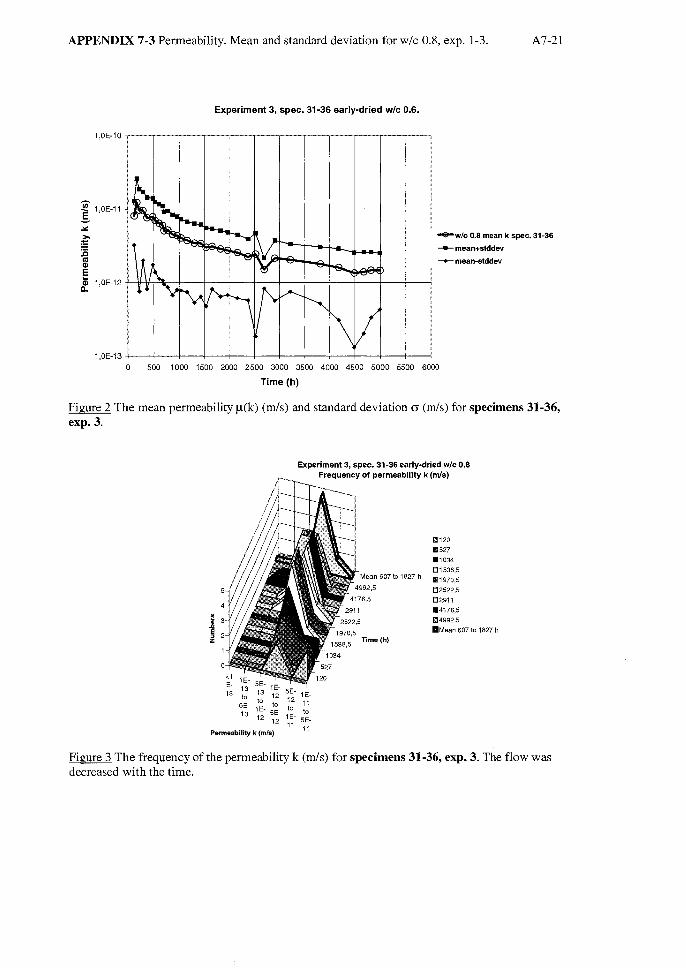
APPENDIX 7-3 Penneability. Mean and standard deviation for w/c 0.8, expo 1-3. A7-21
Experiment 3, spec. 31-36 early-dried wIe 0.6.
i 1,OE-11 +-l~-+= .... -+--t---+--+--t--j--j--f--+--+--!
.lO:
~ -wIe 0.8 mean k spee. 31-36
~ -+-mean+slddev
--+-mean-slddev
E :. 1,OE-12 -J-1Hi'-f-"'''=-+-+-+--+--+--+--+---j--f--f------l
1,OE-13 -J--+---+---+--+--+--+--t--j--j--f--+----i o 500 1000 1500 2000 2500 3000 3500 4000 4500 5000 5500 6000
Time (h)
Figure 2 The mean penneability f-l(k) (mls) and standard deviation (j (mls) for specimens 31-36, exp.3.
Experiment 3, spec. 31-36 early-dried wIe 0.8 Frequeneyof permeability k (mls)
~;- 5E- lE-13 lo 13 12 ~;- lE-
5E- to to 11 13 lE- 5E- lo lo
12 12 ~~- 5E-
Penneoblllty k (mls) l l
Mean 607 to 1827 h
Time (h)
11120 .527 .1034 01538,5
.1970,5 02522,5 02911 .4176,5 114992,5 aMoan 607 to 1827 h
Figure 3 The frequency of the penneabilityk (mls) for specimens 31-36, expo 3. The flow was decreased with the time.

APPENDIX 7-4 Experiment 2: water flow and content of calcium in drainage water
____ Waterflow (m3/s) -+- Leaching rate Ca (kg/s) -.-Content [Ca] (g/I)
1,OE-06
CI) 10E-0? ~ J
Dl s:: :E
1,OE-08 .., tU
..!! 'O s:: tU
~ 1,OE-09 o ;: ~ :s: 1,OE-10
j , 00 ~
tU s:: 'e 'O
.5 tU
(.)
0,010 c .!! s:: o (.)
1,OE-11 +-----t----+---+---+----+--~---+_---'- 0,001
O 20 40 60 80 100 120 140
Accumulated water flow (liter)
Figure 1 Measured drainage water flow and measured (Ca2+] in the drainage water and calculated leaching rate kg Ca2+ /s for specimen l, expo 2.
____ Waterflow (m3/s) -+- Leaching rate Ca (kg/s) --.!r- Content [Ca] (gli)
A7-22
1,OE-10 -r----r------,------r----,-----y-------y---.,----, 1,000
... CI)
~ 0,100 ~
tU s:: .~
'O
tU (.)
0,010 c .!! s:: o (.)
1,OE-12 +-----f----+----f"'-----+----l------j----+----+ 0,001 0,00 0,05 0,10 0,15 0,20 0,25 0,30 0,35 0,40
Accumulated water flow (liter)
Figure 2 Measured drainage water flow and measured (Ca2+] in the drainage water and calculated leaching rate kg Ca2+ /s for specimen 2, expo 2.

APPENDIX 7-4 Experiment 2: water flow and content of calcium in drainage water
A7-23
...... Waterflow (m3/s) -+-Leaching rate Ca (kgIs) ....... Content [Ca] (gli)
1,OE-08 ,....-----,------,.----..-----.,.-----,------..--..,- 1,000
... ~ ~
== ~ 1,OE-09 ~f----+----+----I-----.r.t;;_:;_;:;;;;;_r___+--_____.,..,..J.".,.....,..,+ 0,100 cP
-~ ! ... "i! ~ ~
Iii .5
== ~ ;s:i 1,OE-10 0,010 ~ w ~
1,OE-11 +-----!-----+----I-----+-----!-----+----'- 0,001 0,0 2,0 4,0 6,0 8,0 10,0 12,0
Accumulated water flow (liter)
Figure 3 Measured drainage water flow and measured (Ca2i in the drainage water and calculated leaching rate kg Ca2+ /s for specimen 3, expo 2 .
...... Waterflow (m3/s) -+-Leaching rate Ca (kg/s) ....... Content [Ca] (gli)
1,OE-08,-----,-----,.-----,----........,.----,------,- 1,000
U
~ I ~ 1,OE-09 -illl1II;------!-----+----t------+-----f-----+ 0,100 cP
-~ ! - "i! ~ ~
Iii ~
== ~ j 1,OE-10 0,010 i ~ 8
1,OE-11 +-----+----f-----+----+-----!-----+ 0,001 0,0 2,0 4,0 6,0 8,0 10,0 12,0
Accumulated water flow (liter)
Figure 4 Measured drainage water flow and measured (Ca2+] in the drainage water and calculated leaching rate kg Ca2+ /s for specimen 4, expo 2.

APPENDIX 7-4 Experiment 2: water flow and content of calcium in drainage water
....... Waterflow (m3/s) -+-Leaching rate Ca (kgls) __ Content [Ca] (gli)
A7-24
1,OE-oa -.------,-----,------,-----,------r------,- 1,000
! 1,OE-09 a-
I a-D) 0,100 CD c :c D)
III () C III "! .!!
" 1,OE-10 " c .5 III
==
III (J
~ 0,010 "5 CD
~ c 1,OE-11 o
(J
1 ,OE-12 ... ----+----+-----+------If----+----+ 0,001 0,0 1,0 2,0 3,0 4,0 5,0 6,0
Accumulated water flow (liter)
Figure 5 Measured drainage water flow and measured [Ca2i in the drainage water and calculated leaching rate kg Ca2+ /s for specimen 5, expo 2 .
...... Waterflow (m3/s) -+- Leaching rate Ca (kg/s) --Content [Ca] (gli)
1,OE-06
~ ~ bar
1,
/~ \ - Hr"". -
1\ r sto~
V ~ 1,OE-07
D) c J 1,OE-oa
" c III
~ 1,OE-09
! 1,OE-10
1,OE-11
..-I
~
rr~
~ ~--f.....--... L.. ~ l\ ,
L-O, ......
....... ~ V -----..
V-d '\ J ----r. o,
o, o 10 20 30 40 50 60 70 ao 90 100 110 120 130
Accumulated water flow (liter)
Figure 6 Measured drainage water flow and measured [Ca2+] in the drainage water and calculated leaching rate kg Ca2+ /s for specimen 6, expo 2.
000
I 100 CD
i .5 f! " .5 ~
010 c ~ 8
001

APPENDIX 7-4 Experiment 2: water flow and content of ca1cium in drainage water
___ Waterflow (m/s) -+-Leaching rate Ca (kg/s) ....... Content [Ca] (gli)
A7-25
1,OE-06 -,:.---,--,.----r--,----r--,----r--,----r---,- 1,000
r stop.
CD 1 ,DE-O? +-=\-~~---+--+===+=~_+~.._~::::!!:::t:==~~=r:_~ i! ~ ~100 :c 1 ,DE-DB __ >r-b1~-\-_+--r-"'k---.::.I......,-I_-_+--_I_--+_--I---__j 0111
~ ~ i i 1 ,OE-09 +---jf---=f"--+~=~~=~,::.=t:;;;:+==t=::!:::::~-~ <3 lE 0,010
i 1 ,OE-10 +---+--+---+---+---+---+---+---+---+---1
1,OE-11 +---+---!---+---!----+---I----+---+---+---+ 0,001
O 50 100 150 200 250 300 350 400 450 500
Accumulated water flow (liter)
Figure 7 Measured drainage water flow and measured (Ca2+] in the drainage water and calculated leaching rate kg Ca2+ /s for specimen 7, expo 2.
___ Waterflow (m/s) -+-Leaching rate Ca (kg/s) ....... Content [Ca] (gli)
1,OE-06 .,.-----r----,-----r-----,----,----.,.-----,.-.,-
~ 1 ,DE-O? t-''''''':::--I--::1I---I----t--'\Ja;;;:;;:t.i=it=:::::j~F==-====i,_j :p :: J ~ ~OOCD :c 1,OE-OB ,. ... I---:-~--__t---_+----+---+---+_---I__j ~ ~ "ii! 'tI 'tI
~ ~ ~ 1,OE-09 ~ lE 0,010 i i ~
1,OE-10 O
1,OE-11 +----+----i-----f----f----i----+----+-...L 0,001
O 50 100 150 200 250 300 350
Accumulated water flow (liter)
Figure 8 Measured drainage water flow and measured (Ca2+] in the drainage water and calculated leaching rate kg Ca2+ /s for specimen .8, expo 2.

APPENDIX 7-4 Experiment 2: water flow and content of calcinm in drainage water
___ Waterflow (m3/s) -- Leaching rate Ca (kg/s) ..... Content [Ca] (g/I)
1,OE-06
CP 1 ,O E-O?
i! 01 C j 1,OE-08
~ ~ 1,OE-09
=t: ~ !: 1,OE-10
1,OE-11
\ j 6to 3 bar
... .. \. "-
~ ,..........
-~ ~
.. ~~ ~ ~ ~ ....
\.
V -.... --...:. ........ ~
o 20 40 60 80 100 120 140 160 180
Accumulated water flow (liter)
r~ ..!
O
O
O
200
Figure 9 Measured drainage water flow and measured [Ca2+] in the drainage water and calculated leaching rate kg Ca2+ /s for specimen 10, expo 2 .
....... Spec.1 --Spec.2 ..... Spec. 3 -+-Spec. 4 -e-Spec. 5
A7-26
,000
I ,100 CP
! Mi! "CI
.5
~ ,010 ~
C 8
,001
10,00 -,------,------,.------,.........-----,.........----...........,
~ 1,00 lP 16 !: CP 01 al c "i! 0,10 "CI
.5 al ()
C .s 0,01 c o ()
0,00+------------r-----------4------------~----------4-----------~
0,01 0,10 1,00 10,00 100,00 1000,00 Accumulated water flow (liter)
Figure 10 Measured [Ca2+] in the drainage water for specimen 1-5, expo 2.

APPENDIX 7-4 Experiment 2: water flow and content of calcium in drainage water
___ Spec.6 -+-Spec. 7 -+-Spec. 8 -+-Spec. 10
~ 1,00 ... 4)
'Iii ii: 4) en os s: 'e 0,10 'O
.5 os (J
E .Sl 0,01 s: o (J
A7-27
O,OO+---------------r-------------~--------------_+--------------~
0,1 1,0 10,0 100,0 1000,0 Accumulated water flow (liter)
Figure Il Measured [Ca2+] in the drainage water for specimen 6-8, 10, expo 2.

APPENDIX 7-4 Experiment 2: water flow and content of calcium in drainage water
Content 01 Ca in drainage water
--?lt-Spec.l -+-Spec.2 -wlill-Spec. 3 -å-Spec. 4 ····i,···Spec. 5 -+-Spec. 6 -I--Spec. 7 --Spec. 8 _ .•• wSpec. 10
10,00 --~
1,00
~N.'.;....j~ 1= #4: 1tJ'...:.~
~ :;; 10 Öl
'" '" .. c: 0,10 '! .., .E tO $ c: o o
0,01
o,ooll------------------~----------------~~----------------~~--------------~~~--------------~ ~01 0,10 1,00 10,00 100,00 1000,00
Accumulated water Ilow (liter)
Figure 12 Measured [Ca2+] in the drainage water for specimen 1-8, 10, exp, 2.

APPENDIX 7-4 Experiment 2: water flow and content of calcium in drainage water
Residual total Ca in solid spec. 1-5 (compared with theoretical 65.5% of cement)
A7-29
.... Spec.1 -+-Spec.2 --Spec. 3 ........ Spec. 4 -El-Spec. 5 -"Ruettgers (1936) -+[Sällström 1966]
~ al E
"I .5 ..
110 2
105
100
id g 8. 95 u~ E ..... ::I ·0 90 S
85
80
~
" ~ ~
1
I--- • r-- -- r----~ o 10 20 30 40 50 60 70 80 90 100 110 120 130 140 150
Accumulated water flow (liter)
Figure 13 EstiInated residual content of total Ca in the leached specimen 1-5, expo 2 at a accumulated flow of water of 0-150 (1). It is estimated as the assumed initial content of total Ca minus the measured, accumulated leaching of Ca in the drainage water.
Residual total Ca in solid spec.1-5 (compared with theoreticaI65.5% of cement)
---Spec.1 -+-Spec.2 --Spec. 3 --Spec. 4 -w-Spec. 5 -..Ruettgers (1936)
III 108,0 c al E 107,0 ·0 al D. III 106,0 .5 ii '"":' 105,0 .. u c al oD. u ~ 104,0 E ..... . g 103,0
S g 102,0 "D
~ 101,0
100,0
I
......... ~ ~ ~
"~
S"
~ -- 1
--.... ~ ~ lJ
--.. ....
----
~
~
O 2 3 4 5 6 7 8 9 10
Accumulated water flow (liter)
Figure 14 Estimated residual content of total Ca in the leached specimen 1-5, expo 2 at a accumulated flow of water of 0-10 (1). It is estimated as the assumed initial content of total Ca minus the measured, accumulated leaching of Ca in the drainage water.

APPENDIX 7-4 Experiment 2: water flow and content of calcium in drainage water
Residual total Ca in solid spec. 1-5 (compared with theoretical 65.5% of cement)
--Spec.1 --Spec.2 -+-Spec. 3 --Spec. 4 ""*""Spec. 5 -e-RueHgers (1936)
A7-30
108,2,.-------r-----..,-------,------,--------, 1/1
ii E
l 1/1
108,1 r=~~~1I~~~~~::i==_--~_i--------1_-------l .5 ii --:- 108,0 t-----+----=::::::~~~~~~==t=~~=-,J+-~~~~===j .. u c ID o D. u..!!! § $107,9 +------t------t------+--..e:::,'"""""':'-31 ..... ~"""'=----__l ·u 1i § 107,8 +------!------f------/-------+-------"lk:::"'--%...j "O
~ 107,7 +------+------1-------1------+-------1
0,0 0,1 0,2 0,3 0,4 0,5
Accumulated water flow (liter)
Figure 15 Estimated residual content of total Ca in the leached specimen 1.5, expo 2 at a accumulated flow of water of 0-0.5 (1). It is estimated as the assumed initial content of total Ca minus the measured, accumulated leaching of Ca in the drainage water.
28
.5 '" 27 ~
O "i' 26 U--:-- () o ID .. D. 25 ii~ ä -; 24 () c E ~ .2 ·u 23 ..!:! ~ as 1/1 ~ 22 !!I
"O
~ 21
20
Residual Ca from Ca(OHh in solid spec.1-5 (compared with theoretical13.1 % of .,
--Spec.1 ....... Spec.2 ....... Spec. 3 ....... Spec. 4 -e-Spec. 5
2 I !
l'5 i
I
\ i ! 4, !
~ ... --'---
!
I o 10 20 30 40 50 60 70 80 90 100
Accumulated water flow Oiter)
Figure 16 Estimated residual content of Ca in Ca(OHHs) in the leached specimen 1-5, expo 2 at a accumulated flow of water of 0-150 (I). It is estimated as the assumed initial content of Ca in Ca(OHHs) minus the measured, accumulated leaching of Ca in the drainage water.

APPENDIX 7-4 Experiment 2: water flow and content of calcium in drainage water
40 O
Residual Ca in solid spec. 6-8,10 (compared with theoreticaI65.5% of cement)
..... Spec.6 --Spec. 7 ...... Spec. 8 --Spec.10
\.
~ --10 ~ ...
6 8
'\. -......... --- 7
50 100 150 200 250 300 350 400
Accumulated water flow (liter)
A7-31
450 500
Figure 17 Estimated -residual content oftotal Ca in the leached specimen 6-8, 10, expo 2 at a accumulated flow of water of 0-500 (1). It is estimated as the assumed initial content of total Ca minus the measured, accumulated leaching of Ca in the drainage water.
Residual Ca in solid spec. 6-8,10
..... Spec.6 --Spec. 7 ...... Spec. 8 --Spec.10
75
lir.
" ~ ~ ~ ~ 10
K I--. K ~ r---
1'---.6 r-..... .--I---r--. --r--- .......
50 O 5 10 15 20 25 30 35 40 45 50
Accumulated water flow (liter)
Figure 18 Estimated residual content of total Ca in the leached specimen 6-8, 10, expo 2 at a accumulated flow of water of O-50 (l). It is estimated as the assumed initial content of total Ca minus the measured, accumulated leaching of Ca in the drainage water.

APPENDIX 7-4 Experiment 2: water now and content of calcium in drainage water
.5 '" ~ 15
O 'ii' eJ--:-/I) I,) as II) .. a. e.!!! 5 .ss g l!! I,) II)
E E :::I .-._ I,) I,) II)
"jj i- -5 iii :::I
'" ·iii ~
-15 O
Residual Ca in solid spec. 6-8,10 (compared with theoretical12% CH of cement)
-e-Spec.6 -+-Spec. 7 ........ Spec. 8 --Spec.10
~Ia. 10
\\ ~""!" 8 ~
6
~ r-
--- 7
50 100 150 200 250 300 350 400 450
Accumulated water flow (liter)
A7-32
I , I
I
500
Figure 19 Estimated residual content of Ca in Ca(OH)z(s) in the leached specimen 6-8, 10, expo 2 at a accumulated flow of water of 0-500 (1). It is estimated as the assumed initial content of Ca in Ca(OH)2(s) minus the measured, accumulated leaching of Ca in the drainage water.

APPENDIX 7-5 Experiment 2: water flow and content of potassium and sodium in drainage water
A7-33
Leaching of K
! DI C
1,OE-06
1,OE-07
___ Waterflow (m3/s) -+-Ieaching rate K (kgls) -+-Content [Kl (gli)
fl 1,OE-08 ~
.m "C
lä ~ 1,OE-09
;;::::
j 1,OE-10
1,OE-11
...
\ 't: i'-. .....
o 2
~ ---
4 6 8 10 12 14 16 18
Accumulated water flow (liter)
Figure 1 Measured drainage water flow and measured concentration of potassiurn in the drainage water and calculated leaching rate kg K+ /s for specimen l, expo 2.
i DI C
)
___ Waterflow (m3/s) -+- Leaching rate K (kg/s) -+-Content [Kl (gli)
1,OE-10~----~-------r------~----~------,-------r------r------~
~ 1,OE-11
~ ;;::::
j
1,OE-12 ..L-__ --1. ___ ..L-__ --..L.. ___ .L..-__ -L.. ___ '--__ -'-__ ---L
20
0,1
0,00 0,05 0,10 0,15 0,20 0,25 0,30 0,35 0,40
Accumulated water flow (liter)
Figure 2 Measured drainage water flow and measured concentration of potassiurn in the drainage water and calculated leaching rate kg r /s for specimen 2, expo 2.
0,4
0,35
0,3
0,25
0,2
0,15
0,1
0,05

APPENDIX 7-5 Experiment 2: water flow and content of potassium and sodium in drainage water
A7-34
1,OE-OB
~ 1,OE-09
Dl c :E u as .!! 't:I 1,OE-10 lä ~ ;;::
~ ;> 1,OE-11
1,OE-12
__ Waterflow (m3/s) -+-Leaching rate Ca (kg/s) ~Content [Kl (g/I)
J 6to3bar'l \. 3taBbar.
.; \
r~ ~ --- -- \ l~ 1 !
..,
h ~ --!----r ---- -...
r--..,... ........ o 2 4 6 B 10 12 14
Accumulated water flow (liter)
Figure 3 Measured drainage water flow and measured concentration of potassium in the drainage water and calculated leaching rate kg K+ /s for specimen 3, expo 2.
--Waterflow (m3/s) -+-Leaching rate K (kg/s) ~Content [Kl (g/I)
1,OE-OB ,--.,---,---,--,-----,---,----.,.----,------r--,.--,----,-
_t ~ 1 ,OE-09 -WI"W"\I ... ~-+--+---+--+---I---+----I---+----If---+---f---I Dl \ ~..... '6io3i;ä;. "\ .13 to 6 bar. 1
~ ~' -~J~·~~~UL.-~~~~. r _ ~ ~ -l -lZ..r-........... ~-+-... ..., ................ ~ 1 ,OE-10 +----1~.-t--+----+--+--I--"''+---I--'''I-: ...... --+--f---+----t
---.
~
': ~---~ ---;> 1,OE-11 +---\+---I---+---=="+-=--+--I---+---f----+--+---I---I
j ~ -----~~-+-+ --r--_ -"'~""r-jt--""
1 ,OE-12 -'-_--'-_--1. __ "--_-'-_-.1. __ 1....-_-"-_--'-_--' __ -'--_-'--_--'
o 2 3 4 5 6 7 B 9 10 11 12
Accumulated water flow (liter)
Figure 4 Measured drainage water flow and measured concentration of potassium in the drainage water and calculated leaching rate kg K+ /s for specimen 4, expo 2.
0,25
0,2 "-al
~ al
0,15 Dl as c "e 't:I
.5 0,1 :.::
1: ~ o (,)
0,05
0,3
0,25
"-al '!ii
0,2 ;;: al Dl as c "!
0,15 't:I
.5 :.::
0,1 1: ~ o (,)
0,05

APPENDIX 7-5 Experiment 2: water now and content ofpotassium and sodium in drainage water
1,OE-08
~ 1,OE-09
~
) "C 1,OE-10 Iii ~ :;::
~ > 1,OE-11
1,OE-12
O
....... Waterflow (m3/s) ......... Leaching rate K (kg/s) ...-Content [Kl (gli)
6103 bar. 11
- .. '~ . ...... ... \ (LJ
~ II"F" - - .--- ----~'\ ..... --r~ , -
..
"'" 2 3 4 5
Accumulated water flow (liter)
Figure 5 Measured drainage water flow and measured concentration of potassium in the drainage water and calculated leaching rate kg K+ /s for specimen 5, expo 2 .
1,OE-08
~ 1,OE-09
.0)
.= l i 1,OE-10
~ ~ '!ii == 1,OE-11
1,OE-12
---\~
~
...... Waterflow (m3/s) ......... Ieaching rate K (kg/s) ...-Content [Kl (g/l)
.. -- --- ~
V
~
\' '- -"" "'-~ --.
A7-35
6
0,9
0,8
0,7 Iii '!ii
0,6 ~
0'5·f
"C
0,4.= ~
C 0,3 ~
o 0,2 U
0,1
0,1
0,09
0,08 ... 0,07 j 0,06 ~
C
"! 0,05 "C
.= 0,04 ~
0,031
<3 0,02
0,01
O 2 3 4 5 6 7 8 9 10
Accumulated water flow (liter)
Figure 6 Measured drainage water flow and measured concentration of potassium in the drainage water and calculated leaching rate kg K+ /s for specimen 6, expo 2.

APPENDIX 7-5 Experiment 2: water flow and content of potassium and sodium in drainage water
A7-36
1,OE-07
i 1,OE-08
CII c :c j "CI 1 ,OE-09 Ii ~
;;:::
j :> 1,OE-10
1,OE-11
o
-+-Waterflow (m/s) -+-Ieaching rate K (kg/s) -a-Content [Kl (gli)
\ -------~
~ ~ ...-- \~ ~
\ ~\ ~ ---. ~ ... ~ - -
2 4 6 8 10 12 14 16 18 20
Accumulated water flow (liter)
Figure 7 Measured drainage water flow and measured concentration of potassium in the drainage water and calculated leaching rate kg K+ /s for specimen 7, expo 2.
1,OE-07
~ 1,OE-08 ... CII c
j l1,OE-09
~ j :> 1,OE-10
1,OE-11
o
_+_Waterflow (m/s) -+-Ieaching rate K (kg/s) -a-Content [Kl (gli)
\ / ~
\~ ~ ""'- ---~~
\ \
..... -............ 1\
r--... --..:::;
2 3 4 5 6 7 8 9 10
Accumulated water flow (liter)
Figure 8 Measured drainage water flow and measured concentration of potassium in the drainage water and calculated leaching rate kg K+ /s for specimen 8, expo 2.
0,045
0,035 .. II '!;j
003 ;: , i 0,025 _!
"CI
0,02 .5 ~
0,015 ~ §
0,01 (.)
0,005
0,05
0,045
0,04
0,01
0,005

APPENDIX 7-5 Experiment 2: water flow and content of potassium and sodium in drainage water
1,OE-07
~ 1,OE-08
~
I " 1,OE-09 Ii ~
;;::
j 1,OE-10
1,OE-11
___ Waterflew (m3/s) --Ieaching rate K (kg/s) ....... Centent [Kl (g/I)
\ .~ ---- ~ -- r--
-_.~
~ ~ ~ o 2 3 4
Accumulated water flow (liter)
Figure 9 Measured drainage water flow and measured concentration of potassium in the drainage water and calculated leaching rate kg K+ /s for specimen 10, expo 2.
___ Spec.1 --Spec.2 ....... Spec. 3 ....... Spec. 4 -s-Spec. 5
A7-37
5
0,12
0,1
i 1;j
0,08 ~
.f 0,06 ~
.5 ~
0,04 i
0,02
1: o (,,)
10,00 -,---------r--------,---------,----------,
~
I CD DI III c "! " .5 ~
1: J!! c o (,,)
1,00
0,10
0,01
0,00 +--------+-------+--------+---------1 0,01 0,10 1,00
Accumulated water flow (liter) 10,00 100,00
Figure 10 Measured concentration of potassium in the drainage water for specimen 1-5, expo 2.

APPENDIX 7-5 Experiment 2: water flow and content of potassinm and sodium in drainage water
....... Spec.6 -+-Spec. 7 ..... Spec. 8 --Spec.10
~ 1,00 ... al
"tU
== al al as c 'iii 0,10 ... "O
.5 as (J
c .!! 0,01 c o (J
A7-38
0,00 +-----------1------------1------------1 0,1 1,0 10,0 100,0
Accumulated water flow (liter)
Figure 11 Measured concentration of potassium in the drainage water for specimen 6-8, 10, expo 2.
1,2
:§ 5i 1,0 E 2 .~
~ 0,8
.5 lw:: 'ö 0,6 c ~ 8 0,4
1& ::3
~ 0,2 t!
0,0
°
Residual K in spec.1-5 compared with teoretical 0.57%K20*cement
___ Spec.1 ...... Spec.2 ..... Spec. 3 -+-Spec. 4 -e-Spec. 5
~5 ~
~ 1
--
20 40 60 80 100 120 140
Accumulated water flow (liter)
Figure 12 Residual content of K in specimens 1 to 5 in experiment 2. Spec. 2,5: virgin wie 0.8. Spec. 1,2-3: Late-dried wie 0.8. The initial value is based on information from the cement supplier. The dots in the figure are measured values and the curve between is an interpolation. The last dot in each curve in the figure is extrapolated values. These last values can perhaps be overestimated especially when the drainage water flow was high.

APPENDIX 7-5 Experiment 2: water flowand content of potassium and sodium in drainage water
Residual Na in spec. 1-5 (compared with teoretical 0.05%Na20*Cement)
-ll-Spec.1 -+-Spec.2 ..... Spec. 3 ....... Spec. 4 -a-Spec. 5
0,10
-.9 c al E ·u al t:I. 0,00 III
.5 01 z ... o C al g -0,10 u iij ~
:2 III al II:
-0,20
° 2 4 6 8 10 12 14 16
Accumulated water flow (liter)
A7-39
18 20
Figure 13 Residual content of K in specimens 6 to 8 and 10 in experiment 2. Spec. 10: virgin wie 1.3. Spec. 6-8: Late-dried wie 1.3. The initial value is due to the cement supplier. The dots in the figure are measured values and the curve between is an interpolation_ The last dot in each curve in the figure is extrapolated values. These last values are probably overestimated especially when the drainage water flow was high. There can be no negative concentrations.

APPENDIX 7-5 Experiment 2: water Dow and content of potassinm and sodinm in drainage water
Leaching of Na
Residual S in spec. 1-5 (compared with teoreticaI2.07S030/0*Cement)
...... Spec.1 __ Spec.2 ....... Spec. 3 ----Spec. 4 -s-Spec. 5
A7-40
3,90,-----,-----,-----,-----,------,-----,-----,-----,-------r-----,
$ c al E
13,80 r~,1==~:±~~J---L--L--J---l--J---L---l .5 t/)
'ö
i 8 3,70 +----+----+--~--~~:__:_..._+----t----+--=-t""'""'=-t__----I 3 g
'tI
i 3,60 .L.... ____ ...1-____ ...J...... ____ ....1.... ____ ...J.... ____ -'-____ ...J.... ____ .....J.... ____ --L. ____ .....J.. ____ ......J
O 2 4 6 8 10 12 14 16 18 20
Accumulated water flow (liter)
Figure 14 Residual content ofNa in specimens l to 5 in experiment 2. Spec. 2,5: virgin w/c 0.8. Spec. 1,2-3: Late-dried wie 0.8. The initial value is due to the cement supplier. The dots in the figure are measured values and the curve between is an interpolation. The last dot in each curve in the figure is extrapolated values. These last values are probably overestimated, especially when the drainage water flow was high.

APPENDIX 7-6 Experiment 2: Content of sulphate in drainage water A7-41
Residual S in spec. 1-5 (compared with teoreticaI2.01S03%*Cement)
...... Spec.1 -+-Spec.2 .....-Spec. 3 ....... Spec. 4 -e-Spec. 5
3,90 -,----'T"""--....----,----,----,----;-----;-----,----,-----,
-.9 i .5 l3,80~~~:t::~=i~~_J------l-----l------l-----t----_J------l_--__J .5 III
'ö
i 8 3,10+-----~----_+----_4----~~~ __ +_----~----_+--~~-=~--~--~ m 3 :::I
" ~ 3,60~--~--~--~--~--~--~--~--~--~--~
o 2 4 6 8 10 12 14 16 18 20
Accumulated water flow (liter)
Figure 1 Residual content of S in specimens 1 to 5 in experiment 2. Spec. 2,5: virgin w/c 0.8. Spec. 1, 2-3: Late-dried w/c 0.8. The initial value is due to the cement supplier. The dots in the figure are measured values and the curve between is an interpolation. The last dot in each curve in the figure is extrapolated values. These last values can perhaps be overestimated especially when the drainage water flow was high.

APPENDIX 7-7 Experiment 2: summary of the content of studied elements Ca, K, Na, S and pH in drainage water
A7-42
---Content [I<] (gli) -+-Content [Na] (gli) ....... Content [S] (gli) --Content [Ca] (gli) -e-pH
14 CD CIl al 12 c "i! 6to 3 'tI bar ..
10 CD .5 0,1 ~ aI_ eJ 'ä, 8 CD
CIl 'ti_ llS Ii ~ c
cnfti 6 "i! C i!: 'tI Z 0,01 .5 )[ 4 ::t:
'2 a.
,el 2 c o C)
0,001 ° ° 10 100 1000
Accumulated water flow (liter)
Figure 1 Content of K, Na, S, Ca and W in the drainage water for specimen l, expo 2. The dots in the figure are measured values and the curves between are interpolations.
---Content [K] (gli) -+-Content [Na] (gli) ....... Content [S] (gli) --Content [Ca] (gli) -e-pH
~----::~:t~::~~==~:::;~==~~;;~===r~--------r13,4 13,3
13,2
0,1 L--~=j~[===!===::==c:::::::!:==d~----j 13,1 ~ i!:
13 t 12,9 ~
.5 0,01 t----I--4;:::==te===:::::e7""'0--1\--~tt---~-i 12,8 i
12,7
12,6
0,001 +------!-------I-----+------+-----+ 12,5 0,00 0,05 0,10 0,15 0,20 0,25
Accumulated water flow (liter)
Figure 2 Content of K, Na, S, Ca and W in the drainage water for specimen 2, expo 2. The dots in the figure are measured values and the curves between are interpolations.

APPENDIX 7-7 Experiment 2: summary of the content of studied elements Ca, K, Na, S and pH in drainage water
A7-43
___ Centent [K] (gli) __ Centent [Na] (gli) -+-Centent [S] (gli) --Centent [Ca] (gli) -a-pH
13,6
CD 01 1'11 13,4 c 0i! "el :u .5 0,1 13,2 ; ~E' CD "el 01 01 c~
13 1'11
1'11 :u c CIl1ä 'i! ai:: "el
z 0,01 128.5 '>i ' :c C
Il.
~ 12,6 o o
0,001 12,4 0,0 1,0 2,0 3,0 4,0 5,0 6,0 7,0 8,0 9,0 10,0 11,0
Accumulated water flow (liter)
Figure 3 Content of K, Na, S, Ca and If" in the drainage water for specimen 3, expo 2. The dots in the figure are measured values and the curves between are interpolations.
___ Centent [K] (gli) --Centent [Na] (gli) -+-Centent [S] (gli) --Centent [Ca] (gli) -a-pH
0,1 +---~----_r--~+_--~+---_r----+_--~-----+-7~~--~
.5 0,01 +----\-1'----_r----+_--~'=~-+==.:l\d:::::;;,...,..k:::_--___1I_----~--~ c ~ o O
0,001 +---~f---_r----+_--~f----+----+_--__!----_+----_I_--_+
13,4
13,3
13,2
13,1 ... CD
13 ; CD 01
12,9 .~ f!!
"el 12,8.5
:c 12,7 Il.
12,6
12,5
12,4 0,0 1,0 2,0 3,0 4,0 5,0 6,0 7,0 8,0 9,0 10,0
Accumulated water flow (liter)
Figure 4 Content of K, Na, S, Ca and If" in the drainage water for specimen 4, expo 2. The dots in the figure are measured values and the curves between are interpolations.

APPENDIX 7-7 Experiment 2: sunnnary of the content of studied elements Ca, K, Na, S and pH in drainage water
A7-44
___ Content [K] (g/I) --Content [Na] (gli) .... Content [S] (g/l) --Content [Ca] (gli) -e-pH
13,4
13,2 ou C!
13 m c .. 12,8 ~
== 12,6 8,
m c 12,4 ~
.E
"i! "O 0,1 .E
~E' "O C! c-m lP U) 'lä cä== Z
12,2 ~ ~ 0,01 'E ~ 12 o (J
11,8
0,001 11,6 0,0 1,0 2,0 3,0 4,0 5,0
Accumulated water flow (liter)
Figure 5 Content of K, Na, S, Ca and W in the drainage water for specimen 5, expo 2. The dots in the figure are measured values and the curves between are interpolations.
___ Content [K] (g/l) --Content [Na] (g/l) .... Content [S] (g/I) --Content [Ca] (gli) -e-pH
-r-------..,.....-------,-------..,..--------,- 13,5
0,1 +------=-+-------+--~~---+---------__4
0,01 +------~+----~~-+----~~~~r_--------__4
13
! 125 == , ou
:r c -i! "O
12 .E
11,5
::c 1:1.
0,001 +------~------_1_------+_-----_+ 11 ° 10 100 1000
Accumulated water flow (liter)
Figure 6 Content of K, Na, S, Ca and W in the drainage water for specimen 6, expo 2. The dots in the figure are measured values and the curves between are interpolations.

APPENDIX 7·7 Experiment 2: summary of the content of studied elements Ca, K, Na, S and pH in drainage water
A7-45
el) C! <Il c: 'e -o .5
8=2 -o C! c:~
<Il ~ Ul'lä .r:= z ~ 'E ~ o
"
___ Content [K] (g/I) -+- Content [N a] (g/I) __ Content [S] (g/I) --Content [Ca] (g/I) -e- pH
0,1
0,01
0,001
12,8
12,6
12,4 ...
~ 12,2 ! 12 ~ 'e
-o 11,8.5
J: 11,6 Il.
11,4
11,2
+-------------+_--------~--~nL----------+_------------+11
o 10
Accumulated water flow (liter)
100 1000
Figure 7 Content of K, Na, S, Ca and Jr in the drainage water for specimen 7, expo 2. The dots in the figure are measured values and the curves between are interpolations.
___ Content [K] (g/I) -+- Content [N a] (gli) __ Content [S] (g/I) --Content [Ca] (g/I) -e- pH
0,1 +------------------T----------~----~----------------~
12,8
12,6
12,4 ~ 'lä
122 := , el)
C!
12 ll! 'e -o
11,8 .5 0,01 +-------------''''''---=:::~'--t------------------_t_IrI'_------''T__------__j ;
11,6 -
11,4
11,2
0,001 +----------'----'-+---------1----------1- 11
10 100 1000
Accumulated water flow (liter)
Figure 8 Content of K, Na, S, Ca and Jr in the drainage water for specimen 8, expo 2. The dots in the figure are measured values and the curves between are interpolations.

APPENDIX 7-7 Experiment 2: summary of the content of studied elements Ca, K, Na, S and pH in drainage water
A7-46
III al ca c -i!
'tI
.5
8~ 'tIal c-
c:! cG~ z
':!tI!.-
t: ~ o o
....... Content [K] (g/l) --Content [Na] (gli) ....... Content [S] (g/l) --Content [Ca] (gli) -e-pH
0,1
0,01
0,001
13
12,8
12,6 .. +-----~~--~------------~--~~ __ ----+_----------_4 l
124 ~ , III
i 12,2.5
l! 12 ~
::c 11,8 g.
11,6
11,4
+-----------~------------~------------+_----------__+11,2
O 10 100 1000
Accumulated water flow (liter)
Figure 9 Content of K, Na, S, Ca and W in the drainage water for specimen 10, expo 2. The dots in the figure are measured values and the curves between are interpolations.

APPENDIX 7-8 Experiment 2: stress-strain curves of drilled-ont cores A7-47
50,00
40,00 'ii o.. e III III 30,00 l!! "Iii c o ·iii
20,00 III l!! o.. E o (.)
10,00
0,00 0,0
50,00
40,00 'ii o.. e III III 30,00 l!! "Iii c o ·iii
20,00 III l!! o.. E o (.)
10,00
0,00 0,0
Compression test Specimen 1 (Ia~ried wlc 0.8), Experiment 2.
1,0 2,0 3,0
Deformation (mm)
141.42 mm
4,0
~Leached specimen 1a
-+-Leached specimen 1 b
""*-Not leached specimen 1 aR
_ Not leached specimen 1 bR
5,0
Compression test Specimen 3 (Iate-dried wie 0.8), experiment 2.
1,0 2,0 3,0
Deformation (mm)
4,0
~ Leached specimen 3a
-+-Not leached specimen 3aR
-.... Not leached specimen 3bR
_Not leached specimen 3cR
5,0

APPENDIX 7-8 Experiment 2: stress-strain curves of driIled-out cores A7-48
Compression test Specimen 6 (Iate-dried wie 1.3), experiment 2.
20,00 -r-----~:-;~--r----_r----.,....---_.
l 15,00 +-----;~---;j.+---~-".!__''''---+_----+_---___l
e
I 6 1 0,00 +-___ -1IIF--.l-~----+_-~;:_'.;-__i
.~ r::I. E <3 5,00 +-it--l __ ~-+-----+_----I
t3842
rm
___ Leached specimen Sa
-t-Laached specimen 6b
-A-Not leached specimen 6aR
_ Not leached specimen abR
0,00~"~----~-------+-------~--------+--------4
0,0
25,00
20,00 "ii a.. e /II /II 15,00 l!! '!ii c o 'iii
10,00 el r::I. E o U
5,00
0,00 0,0
1,0 2,0 3,0
Deformation (mm)
4,0 5,0
Compression test Specimen 8 (Iate-dried wie 1.3), experiment 2.
1,0 2,0 3,0
Deformation (mm)
139.41 mm
4,0
_ Leaced specimen 8a
.....-Not leached specimen BaR
"""'Å-Not leached specimen abR
5,0

APPENDIX 7-8 Experiment 2: stress-strain curves of drilled-out cores A7-49
Compression test Specimen 10 (virgin wlc 1,3), experiment 2.
30,00 -,-----......,.--------.......,----...,----.......,
25,00 +----~~ __ ---+----_+_----+_---___l
'l e.. 20,00 +---:::::lF--:=-+---~+-----I----+-----I II! i C 15,00 t-"Ib~"P~~=-+---"",--j .2 fl)
~ ~ 10,00 +-::IIi~ ... -I------t~"""':----l
8
_ Leached specimen 1 Da
/----___ -+-Leached specimen 10b
-..-Not leached specimen 1 DaR l -Not leached specimen 10bR
:~45 1--_----1
5,00 +-=_F---I------+----_+_----'''?-~+_---___l
0,00 0,0 1,0 2,0 3,0
Deformation (mm)
4,0 5,0

I I I I I I I I I I I I I I I I I I I I I I I I I I I I I I I I I I I I I I I I I
I I I I I I I I I I I I I I I I I I I I
I I I I I I I I I I
I I I I I
I I I
I
I I I I

A8-1
APPENDIX TO CHAPTER 8
Leaching rate of calcium and potassium

APPENDIX Experiment 2: Leaching rate calcium and potassium
---Content [Ca] (glI) __ [Ca]=(1/rot[Ca(0))+.15*Q)1I..2 (rate 1.5) -.- [Ca]=[Ca(0)]*(qO/q)A1,5
0,8
S f! 0,6 al C :c j og 0,4 Ii ~ 'E cu 'Iii 02 ;: ,
0,0
\\
\-O 20
/g F 40 60 80 100 120 140
Accumulated water flow (liter)
A8-2
Figure 1 Assumed content of Ca in drainage water compared to measured content for specimen 1, expo 2. The assumed content is calculated with 1); rate = -O.1473[Cat5 or expressed as
[Ca]Q = ( b + k· Q)-2 , and 2); [Ca]=[Ca(O)]*(qO/qt, see chapter 8.3.3 for defInitions. ,,[Ca]o
---Content [Ca] (gli)
1,1
1,0
0,9
0,8
0,7 ~ 'ö 0,6 j 80,5
0,4
0,3
0,2
0,1
0,0
.\
O
, :~ ~ ~
~ r--20 40
-- [Ca]=[Ca(0)]*e"-(0.23*Q) (rate 1.0) -.- [Ca]=[Ca(0)]*(qO/q)AO.6
I
- 16103 bar 1
60 80 100 120 140 160 180 200
Accumulated water flow (liter)
Figure 2 Assumed content of Ca in drainage water compared to measured content for specimen 10, expo 2. The assumed content is calculated with l); a rate = -O.2334[Ca]l.O and a rate =O.9169[Ca]1.5, and 2); [Ca]=[Ca(O)]*(qO/qt, see chapter 8.3.3 for definitions.

APPENDIX Experiment 2: Leaching rate calcium and potassium
~
'ö
0,40
0,30
~ 0,20 1: <3
0,10
0,00
---Content [Kl (g/I)
I~
I\~ ~ i:-'""---
O 2 4
--Assumed 1.5 order rate -.-Assumed 2.0 order rate
6 8 10 12 14 16 18
Accumulated water flow (liter)
A8-3
20
Figure 3 Assumed content of K in drainage water compared to measured content for specimen l, expo 2. The assumed content is calculated with 1); rate = -1. 1 [Kt5 and a rate = 28.8[K]2.0, and 2); [K]=[K(O)]*(qO/q)a, see chapter 8.3.3 for definitions.

KFS AB, Lund 2001