Embed Size (px)
Citation preview

Journal of Mathematical Neuroscience (2013) 3:1DOI 10.1186/2190-8567-3-1
RESEARCH Open Access
Laws of Large Numbers and Langevin Approximationsfor Stochastic Neural Field Equations
Martin G. Riedler ·Evelyn Buckwar
Received: 4 July 2012 / Accepted: 14 January 2013 / Published online: 23 January 2013© 2013 M.G. Riedler, E. Buckwar; licensee Springer. This is an Open Access article distributed under theterms of the Creative Commons Attribution License (http://creativecommons.org/licenses/by/2.0), whichpermits unrestricted use, distribution, and reproduction in any medium, provided the original work isproperly cited.
Abstract In this study, we consider limit theorems for microscopic stochastic mod-els of neural fields. We show that the Wilson–Cowan equation can be obtained as thelimit in uniform convergence on compacts in probability for a sequence of micro-scopic models when the number of neuron populations distributed in space and thenumber of neurons per population tend to infinity. This result also allows to obtainlimits for qualitatively different stochastic convergence concepts, e.g., convergencein the mean. Further, we present a central limit theorem for the martingale part ofthe microscopic models which, suitably re-scaled, converges to a centred Gaussianprocess with independent increments. These two results provide the basis for pre-senting the neural field Langevin equation, a stochastic differential equation takingvalues in a Hilbert space, which is the infinite-dimensional analogue of the chemicalLangevin equation in the present setting. On a technical level, we apply recently de-veloped law of large numbers and central limit theorems for piecewise deterministicprocesses taking values in Hilbert spaces to a master equation formulation of stochas-tic neuronal network models. These theorems are valid for processes taking values inHilbert spaces, and by this are able to incorporate spatial structures of the underlyingmodel.
Keywords Stochastic neural field equation · Wilson–Cowan model · Piecewisedeterministic Markov process · Stochastic processes in infinite dimensions · Law oflarge numbers · Martingale central limit theorem · Chemical Langevin equation
Mathematics Subject Classification (2000) 60F05 · 60J25 · 60J75 · 92C20
M.G. Riedler (�) · E. BuckwarInstitute for Stochastics, Johannes Kepler University, Linz, Austriae-mail: [email protected]
E. Buckware-mail: [email protected]

Page 2 of 54 M.G. Riedler, E. Buckwar
1 Introduction
The present study is concerned with the derivation and justification of neural fieldequations from finite size stochastic particle models, i.e., stochastic models for thebehaviour of individual neurons distributed in finitely many populations, in terms ofmathematically precise probabilistic limit theorems. We illustrate this approach withthe example of the Wilson–Cowan equation
τ ν(t, x) = −ν(t, x) + f
(∫D
w(x, y)ν(t, y)dy + I (t, x)
). (1.1)
We focus on the following two aspects:
(A) Often one wants to study deterministic equations such as Eq. (1.1) in order toobtain results on the ‘behaviour in the mean’ of an intrinsically stochastic sys-tem. Thus, we first discuss limit theorems of the law of large numbers type forthe limit of infinitely many particles. These theorems connect the trajectories ofthe stochastic particle models to the deterministic solution of mean field equa-tions, and hence provide a justification studying Eq. (1.1) in order to infer on thebehaviour of the stochastic system.
(B) Secondly, we aim to characterise the internal noise structure of the complex dis-crete stochastic models as in the limit of large numbers of neurons the noise isexpected to be close to a simpler stochastic process. Ultimately, this yields astochastic neural field model in terms of a stochastic evolution equation concep-tually analogous to the Chemical Langevin Equation. The Chemical LangevinEquation is widely used in the study of chemical reactions networks for whichthe stochastic effects cannot be neglected but a numerical or analytical study ofthe exact discrete model is not possible due to its inherent complexity.
In this study, we understand as a microscopic model a description as a stochastic pro-cess, usually a Markov chain model, also called amaster equation formulation (cf. [3,5, 8, 9, 22] containing various master equation formulations of neural dynamics). Incontrast, amacroscopic model is a deterministic evolution equation such as (1.1). De-terministic mean field equations have been used widely and for a long time to modeland analyse large scale behaviour of the brain. In their original deterministic form,they are successfully used to model geometric visual hallucinations, orientation tun-ing in the visual cortex and wave propagation in cortical slices to mention only a fewapplications. We refer to [7] for a recent review and an extensive list of references.The derivation of these equations is based on a number of arguments from statisti-cal physics and for a long time a justification from microscopic models has not beenavailable. The interest in deriving mean field equations from stochastic microscopicmodel has been revived recently as it contains the possibility to derive deterministic‘corrections’ to the mean field equations, also called second-order approximations.These corrections might account for the inherent stochasticity, and thus incorporateso called finite size effects. This has been achieved by either applying a path-integralapproach to the master equation [8, 9] or by a van Kampen system-size expansion ofthe master equation [5]. In more detail, the author in the latter reference proposes aparticular master equation for a finite number of neuron populations and derives the

Journal of Mathematical Neuroscience (2013) 3:1 Page 3 of 54
Wilson–Cowan equation as the first-order approximation to the mean via employingthe van Kampen system size expansion and then taking the continuum limit for a con-tinuum of populations. In keeping also the second-order terms, a ‘stochastic’ versionof the mean field equation is also presented in the sense of coupling the first momentequation to an equation for the second moments.
However, the van Kampen system size expansion does not give a precise math-ematical connection, as it neither quantifies the type of convergence (quality of thelimit), states conditions when the convergence is valid nor does it allow to charac-terise the speed of convergence. Furthermore, particular care has to be taken in sys-tems possessing multiple fixed points of the macroscopic equation, and we refer to[5] for a discussion of this aspect in the neural field setting. The limited applicabil-ity of the van Kampen system size expansion was already well known to Sect. 10 invan Kampen [33]. In parallel to the work of van Kampen, T. Kurtz derived preciselimit theorems connecting sequences of continuous time Markov chains to solutionsof systems of ordinary differential equations; see the seminal studies [19, 20] or themonograph [15]. Limit theorems of that type are usually called the fluid limit, ther-modynamic limit, or hydrodynamic limit; for a review, see, e.g., [13].
As is thoroughly discussed in [5] establishing the connection between masterequation models and mean field equations involves two limit procedures. First, alimit which takes the number of particles, in this case neurons per considered popu-lation, to infinity (thermodynamic limit), and a second which gives the mean field bytaking the number of populations to infinity (continuum limit). In this ‘double limit’,the theorems by Kurtz describe the connection of taking the number of neurons perpopulation to infinity yielding a system of ordinary differential equation, one for eachpopulation. Then the extension from finite to infinite dimensional state space is ob-tained by a continuum limit. This procedure corresponds to the approach in [5]. Thus,taking the double limit step by step raises the question what happens if we first takethe spatial limit and then the fluid limit, thus reversing the order of the limit proce-dures, or in the case of taking the limits simultaneously. Recently, in an extension tothe work of Kurtz, one of the present authors and co-authors established limit the-orems that achieve this double limit [27], thus being able to connect directly finitepopulation master equation formulations to spatio-temporal limit systems, e.g., par-tial differential equation or integro-differential equations such as the Wilson–Cowanequation (1.1). In a general framework, these limit theorems were derived for Piece-wise Deterministic Markov Processes on Hilbert spaces, which in addition to thejump evolution also allow for a coupled deterministic continuous evolution. Thisgenerality was motivated by applications to neuron membrane models consisting ofmicroscopic models of the ion channels coupled to a deterministic equation for thetransmembrane potential. We find that this generality is also advantageous for thepresent situation of a pure jump model as it allows to include time-dependent inputs.In this study, we employ these theorems to achieve the aims (A) and (B) focussing onthe example of the deterministic limit given by the Wilson–Cowan equation (1.1).
Finally, we state what this study does not contain, which in particular distinguishesthe present study from [5, 8, 9] beyond mathematical technique. Presently, the aim isnot to derive moment equations, i.e., a deterministic set of equations that approximatethe moments of the Markovian particle model, but rather processes (deterministic or

Page 4 of 54 M.G. Riedler, E. Buckwar
stochastic) to which a sequence of microscopic models converges under suitable con-ditions in a probabilistic way. This means that a microscopic model, which is closeto the limit—presently corresponding to a large number of neurons in a large num-ber of populations—can be assumed to be close to the limiting processes in structureand pathwise dynamics as indicated by the quality of the stochastic limit. Hence, thepresent work is conceptually—though neither in technique nor results—close to [30]wherein using a propagation to chaos approach in the vicinity of neural field equa-tions the author also derives in a mathematically precise way a limiting process tofinite particle models. However, it is an obvious consequence that the convergence ofthe models necessarily implies a close resemblance of their moment equations. Thisprovides the connection to [5, 8, 9], which we briefly comment on in Appendix B.
As a guide, we close this introduction with an outline of the subsequent sectionsand some general remarks on the notation employed in this study. In Sects. 1.1 to 1.3,we first discuss the two types of mean field models in more detail, on the one hand,the Wilson–Cowan equation as the macroscopic limit and, on the other hand, a masterequation formulation of a stochastic neural field. The main results of the paper arefound in Sect. 2. There we set up the sequence of microscopic models and stateconditions for convergence. Limit theorems of the law of large numbers type arepresented in Theorem 2.1 and Theorem 2.2 in Sect. 2.1. The first is a classical weaklaw of large numbers providing uniform convergence on compacts in probability andthe second convergence in the mean uniformly over the whole positive time axis.Next, a central limit theorem for the martingale part of the microscopic models ispresented in Sect. 2.2 characterising the internal fluctuations of the model to be ofa diffusive nature in the limit. This part of the study is concluded in Sect. 2.3 bypresenting the Langevin approximations that arise as a result of the preceding limittheorems. The proofs of the theorems in Sect. 2 are deferred to Sect. 4. The studyis concluded in Sect. 3 with a discussion of the implications of the presented resultsand an extension of these limit theorems to different master equation formulations ormean field equations.
Notations and Conventions Throughout the study, we denote by Lp(D), 1 ≤ p ≤∞, the Lebesgue spaces of real functions on a domain D ⊂ R
d , d ≥ 1. Physicallyreasonable choices are d ∈ {1,2,3}, however, for the mathematical theory presentedthe spatial dimension can be arbitrary. In the present study, spatial domains D arealways bounded with a sufficiently smooth boundary, where the minimal assumptionis a strong local Lipschitz condition; see [2]. For bounded domains D, this condi-tion simply means that for every point on the boundary its neighbourhood on theboundary is the graph of a Lipschitz continuous function. Furthermore, for α ∈ N
we denote by Hα(D) the Sobolev spaces, i.e., subspaces of L2(D), with the corre-sponding Sobolev norm. For α ∈ R+\N we denote by Hα(D) the interpolating Besovspaces. In this study, H−α(D) is the dual space of Hα(D), which is in contrast to thewidespread notation to denote by H−α(D), α ≥ 0, the dual space of Hα
0 (D). Asusual, we have H 0(D) = L2(D) = H−0(D). We thus obtain a continuous scale ofHilbert spaces Hα(D), α ∈ R, which satisfy that Hα1(D) is continuously embed-

Journal of Mathematical Neuroscience (2013) 3:1 Page 5 of 54
ded1 in Hα2(D) for all α1 < α2. Next, a pairing (·, ·)Hα denotes the inner productof the Hilbert space Hα(D) and pairings in angle brackets 〈·, ·〉Hα denote the dualitypairing for the Hilbert space Hα(D). That is, for ψ ∈ Hα(D) and φ ∈ H−α(D) theexpression 〈φ,ψ〉Hα denotes the application of the real, linear functional φ to ψ . Fur-thermore, the spaces Hα(D), L2(D) and H−α(D) form an evolution triplet, i.e., theembeddings are dense and the application of linear functionals and the inner productin L2(D) satisfy the relation
〈φ,ψ〉Hα = (φ,ψ)L2 ∀φ ∈ L2(D),ψ ∈ Hα(D). (1.2)
Norms in Hilbert spaces are denoted by ‖ · ‖Hα , ‖ · ‖0 is used to denote the supremumnorm of real functions, i.e., for f : R → R we have ‖f ‖0 = supz∈R |f (z)|, and | · |denotes either the absolute value for scalars or the Lebesgue measure for measurablesubsets of Euclidean space. Finally, we use N0 to denote the set of integers includingzero.
1.1 The Macroscopic Limit
Neural field equations are usually classified into two types: rate-based and activity-based models. The prototype of the former is the Wilson–Cowan equation; seeEq. (1.1), which we also restate below, and the Amari equation, see Eq. (3.7) inSect. 3, is the prototype of the latter. Besides being of a different structure, due totheir derivation, the variable they describe has a completely different interpretation.In rate-based models, the variable describes the average rate of activity at a certainlocation and time, roughly corresponding to the fraction of active neurons at a certaininfinitesimal area. In activity-based models, the macroscopic variable is an averageelectrical potential produced by neurons at a certain location. For a concise physicalderivation that leads to these models, we refer to [5]. In the following, we considerrate-based equations, in particular, the classical Wilson–Cowan equation, to discussthe type of limit theorems we are able to obtain. We remark that the results are essen-tially analogous for activity based models.
Thus, the macroscopic model of interest is given by the equation
τ ν(t, x) = −ν(t, x) + f
(∫D
w(x, y)ν(t, y)dy + I (t, x)
), (1.3)
where τ > 0 is a decay time constant, f : R → R+ is a gain (or response) functionthat relates inputs that a neuron receives to activity. In (1.3), the value f (z) can beinterpreted as the fraction of neurons that receive at least threshold input. Further-more, w(x,y) is a weight function, which states the connectivity strength of a neuronlocated at y to a neuron located at x, and finally, I (t, x) is an external input, whichis received by a neuron at x at time t . For the weight function w : D × D → R andthe external input I , we assume that w ∈ L2(D × D) and I ∈ C(R+,L2(D)). As for
1A normed space X is continuously embedded in another normed space Y , in symbols X ↪→ Y , if X ⊂ Y
and there exists a constant K < ∞ such that ‖u‖Y ≤ K‖u‖X for all u ∈ X.

Page 6 of 54 M.G. Riedler, E. Buckwar
the gain function f , we assume in this study that f is non-negative, satisfies a globalLipschitz condition with constant L > 0, i.e.,∣∣f (a) − f (b)
∣∣≤ L|a − b| ∀a, b ∈ R, (1.4)
and it is bounded. From an interpretive point-of-view, it is reasonable and con-sistent to stipulate that f is bounded by one—being a fraction—as well as beingmonotone. The latter property corresponds to the fact that higher input results inhigher activity. In specific models, f is often chosen to be a sigmoidal function, e.g.,f (z) = (1 + e−(β1z+β2))−1 in [6] or f (z) = (tanh(β1z + β2) + 1)/2 in [3], whichboth satisfy f ∈ [0,1]. Moreover, the most common choices of f are even infinitelyoften differentiable with bounded derivatives, which already implies the Lipschitzcondition (1.4).
The Wilson–Cowan equation (1.3) is well-posed in the strong sense as an integralequation in L2(D) under the above conditions. That is, Eq. (1.3) possesses a unique,continuously differentiable global solution ν to every initial condition ν(0) = ν0 ∈L2(D), i.e., ν ∈ C1([0, T ],L2(D)) for all T > 0, which depends continuously onthe initial condition. Furthermore, if the initial condition satisfies ν0(x) ∈ [0,‖f ‖0]almost everywhere in D, then it holds for all t > 0 that ν(t, x) ∈ (0,‖f ‖0) for almostall x ∈ D. For a brief derivation of these results, we refer to Appendix A where wealso state a result about higher spatial regularity of the solution: Let α ∈ N be suchthat α > d/2. If now ν0 ∈ Hα(D) and if f is at least α-times differentiable withbounded derivatives and the weights and the input function satisfy w ∈ Hα(D × D)
and I ∈ C(R+,Hα(D)), then the equation is well-posed in Hα(D), i.e., for all T > 0in ν ∈ C1([0, T ],Hα(D)). In particular, this implies that the solution ν is jointlycontinuous on R+ × D.
1.2 Master Equation Formulations of Neural Network Models
For the microscopic model, we concentrate on a variation of the model considered in[5, 6], which is already an improvement on a model introduced in [11]. We extend themodel including variations among neuron populations and foremost time-dependentinputs. We chose this model over the master equation formulations in [8, 9] as it pro-vides a more direct connection of the microscopic and macroscopic models; see alsothe discussion in Sect. 3. We describe the main ingredients of the model beginningwith the simpler, time-independent model as prevalent in the literature. Subsequently,in Sect. 1.3 the final, time-dependent model is defined.
We denote by P the number of neuron populations in the model. Further, we as-sume that the kth neuron population consists of identical neurons which can eitherbe in one of two possible states, active, i.e., emitting action potentials, and inactive,i.e., quiescent or not emitting action potentials. Transitions between states occur in-stantaneously and at random times. For all k = 1, . . . ,P , the random variables Θk
t
denote the number of active neurons at time t . An integer l(k) is used to characterisethe population size. This number l(k) can be interpreted as the number of neurons inthe kth population, at least for sufficiently large values. However, this is not accuratein the literal sense as it is possible with positive probability for populations to containmore than l(k) active neurons. Nevertheless, a posteriori the interpretation can be sal-

Journal of Mathematical Neuroscience (2013) 3:1 Page 7 of 54
vaged from the obtained limit theorems.2 It is a corollary of these that the probabilityof more then l(k) neurons being active for some time becomes arbitrarily small forlarge enough l(k). Hence, for physiological reasonable neuron numbers the probabil-ity in these models of observing ‘non-physiological’ trajectories in the interpretationbecomes ever smaller.
Proceeding with notation, Θt = (Θ1t , . . . ,ΘP
t ) is a (unbounded) piecewise con-stant stochastic process taking values in N
P0 . The stochastic transitions from inactive
to active states and vice versa for a neuron in population k are governed by a con-stant inactivation rate τ−1 > 0—uniformly for all populations—and inputs from otherneurons depending on the current network state. This non-negative activation rate isgiven by τ−1l(k)f k(θ) for θ ∈ N
P0 . For the definition of f k , we consider weights
Wkj , k, j = 1, . . . ,P , which weigh the input one neuron in population k receivesfrom a neuron in population j . Then the activation rate of a neuron in population k isproportional to
f k(θ) = f
(P∑
j=1
Wkjθj
)(1.5)
for a non-negative function f : R → R, which obviously corresponds to the gainfunction f in the Wilson–Cowan equation (1.3). We remark that here f is not therate of activation of one neuron. In this model, the activation rate of a populationis not proportional to the number of inactive neurons but it is proportional to l(k),which stands for the total number of neurons in the population. In [5], this rate is thusinterpreted as the rate with which a neuron becomes or remains active.
It follows that the process (Θt )t≥0 is a continuous-time Markov chain which isusually defined via the following master equation, where ek denotes the kth basisvector of R
P ,
dP[θ, t]dt
= 1
τ
P∑k=1
(l(k)f k(θ − ek)P[θ − ek, t]
− (θk + l(k)f k(θ))P[θ, t] + (θk + 1
)P[θ + ek, t]
)(1.6)
which is endowed with the boundary conditions P[θ, t] = 0 if θ /∈ NP0 . In (1.6), the
variable P[θ, t] denotes the probability that the process Θt is in state θ at time t .Finally, the definition is completed with stating an initial law L, the distribution ofΘ0, i.e., providing an initial value for the ODE system (1.6).
Another definition of a continuous-time Markov chain is via its generator; see,e.g., [15]. Although the master equation is widely used in the physics and chemicalreactions literature the mathematically more appropriate object for the study of aMarkov process is its generator and the master equation is an object derived from
2The derivation of limit theorems for bounded populations sizes, where l(k) actually is the number of neu-rons per population, is much more delicate than the subsequent presentation as the transition rate functionsbecome discontinuous. Although this would be a desirable result, we have not yet been able to prove sucha theorem, though it is clear that the Wilson–Cowan equation would be the only possible limit. See also adiscussion of this aspect in Sect. 3.2.

Page 8 of 54 M.G. Riedler, E. Buckwar
the generator, see Sect. V in [33]. The generator of a Markov process is an operatordefined on the space of real functions over the state space of the process. For theabove model defined by the master equation (1.6), the generator is given by
Ag(θ) = λ(θ)
∫N
P0
(g(ξ) − g(θ)
)μ(θ,dξ) (1.7)
for all suitable g : NP0 → R. For details, we refer to [15]. Here, λ is the total instanta-
neous jump rate, given by
λ(θ) := 1
τ
P∑k=1
(θk + l(k)f k(θ)
), (1.8)
and defines the distribution of the waiting time until the next jump, i.e.,
P[Θt+s = Θt ∀s ∈ [0,Δt]|Θt = θ
]= e−λ(θ)Δt .
Further, the measure μ in (1.7) is a Markov kernel on the state space of the processdefining the conditional distribution of the post-jump value, i.e.,
P[Θt ∈ A|Θt �= Θt−] = μ(Θt−,A) (1.9)
for all sets A ⊆ NP0 . In the present case for each θ , the measure μ is given by the
discrete distribution
μ(θ, {θ − ek}
)= 1
τ
θk
λ(θ),
μ(θ, {θ + ek}
)= 1
τ
l(k)f k(θ)
λ(θ)∀k = 1, . . . ,P .
(1.10)
The importance of the generator lies in the fact that it fully characterises a Markovprocess and that convergence of Markov processes is strongly connected to the con-vergence of their generators; see [15].
1.3 Including External Time-Dependent Input
Until now, the microscopic model does not incorporate any time-dependent input intothe system. In analogy to the macroscopic equation (1.3), this input enters into themodel inside the active rate function f k . Thus, let I k(t) denote the external input intoa neuron in population k at time t , then the time-dependent activation rate is given by
f k(θ, t) = f
(P∑
j=1
Wkjθj + I k(t)
). (1.11)
The most important qualitative difference when substituting (1.5) by (1.11) is that thecorresponding Markov process is no longer homogeneous. In particular, the waiting

Journal of Mathematical Neuroscience (2013) 3:1 Page 9 of 54
time distributions in between jumps are no longer exponential, but satisfy
P[Θt+s = Θt ∀s ∈ [0,Δt]|Θt = θ
]= e− ∫ Δt0 λ(θ,s)ds .
Hence, the resulting process is an inhomogeneous continuous-time Markov chain;see, e.g., Sect. 2 in [36]. It is straightforward to write down the corresponding masterequation analogously to (1.6) yielding a system of non-autonomous ordinary differ-ential equations, cf. the master equation formulation in [8]. Similarly, there existsthe notion of a time-dependent generator for inhomogeneous Markov processes, cf.Sect. 4.7 in [15]. Employing a standard trick, that is, suitably extending the statespace of the process, we can transform a inhomogeneous to a homogeneous Markovprocess [15, 28]. That is, the space-time process Yt := (Θt , t) is again a homoge-neous Markov process. The initial law of the associated space-time process is L × δ0on N
P × R+. We emphasise that definitions of the space-time process and its initiallaw imply that the time-component starts at 0 a.s. and, moreover, moves continuouslyand deterministically. That is, the trajectories satisfy in between jumps the differentialequation (
θ
t
)=(01
),
where the jump intensity λ is given by the sum of all individual time-dependentrates analogously to (1.8). Finally, the post jump value is given by a Markov ker-nel μ((θ, t), ·)× δt as there clearly do not occur jumps in the progression of time andμ is the obvious time-dependent modification of (1.10).
It thus follows, that the space-time process (Θt , t)t≥0 is a homogeneous PiecewiseDeterministic Markov Process (PDMP); see, e.g., [14, 16, 26]. This connection isparticularly important as we apply in the course of the present study limit theoremsdeveloped for this type of processes; see [27]. Finally, for the space-time process(Θt , t)t≥0, we obtain for suitable functions g : N
P0 × R+ → R the generator
Ag(θ, t) = ∂tg(θ, t) + λ(θ, t)
∫N
P0
(g(ξ, t) − g(θ, t)
)μ((θ, t),dξ
). (1.12)
2 A Precise Formulation of the Limit Theorems
In this section, we present the precise formulations of the limit theorems. To thisend, we first define a suitable sequence of microscopic models, which gives theconnection between the defining objects of the Wilson–Cowan equation (1.3) andthe microscopic models discussed in Sect. 1.2. Thus, (Y n
t )t≥0 = (Θnt , t)t≥0, n ∈ N,
denotes a sequence of microscopic PDMP neural field models of the type as de-fined in Sect. 1.3. Each process (Y n
t )t≥0 is defined on a filtered probability space(Ωn, F n, (F n
t )t≥0,Pn), which satisfies the usual conditions. Hence, the defining ob-
jects for the jump models are now dependent on an additional index n. That is P(n)
denotes the number of neuron populations in the nth model, l(k, n) is the number ofneurons in the kth population of the nth model and analogously we use the notations

Page 10 of 54 M.G. Riedler, E. Buckwar
Wn
kj and I k,n and f k,n. However, we note from the beginning that the decay rate τ−1
is independent of n and τ is the time constant in the Wilson–Cowan equation (1.3).In the following paragraphs, we discuss the connection of the defining componentsof this sequence of microscopic models to the components of the macroscopic limit.
Connection to the Spatial Domain D A key step of connecting the microscopicmodels to the solution of Eq. (1.3) is that we need to put the individual neuron pop-ulations into relation to the spatial domain D the solution of (1.3) lives on. To thisend, we assume that each population is located within a sub-domain of D and thatthe sub-domains of the individual populations are non-overlapping. Hence, for eachn ∈ N, we obtain a collection Dn of P(n) non-overlapping sub-sets of D denotedby D1,n, . . . ,DP(n),n. We assume that each subdomain is measurable and convex.The convexity of the sub-domains is a technical condition that allows us to applyPoincaré’s inequality, cf. (4.1). We do not think that this condition is too restrictiveas most reasonable partition domains, e.g., cubes, triangles, are convex. Furthermore,for all reasonable domainsD, e.g., all Jordan measurable domains, a sequence of con-vex partitions can be found such that additionally the conditions imposed in the limittheorems below are also satisfied. One may think of obtaining the collection Dn bypartitioning the domain into P(n) convex sub-domains D1,n, . . . ,DP(n),n and con-fining each neuron population to one sub-domain. However, it is not required that theunion of the sets in Dn amounts to the full domain D nor that the partitions consistsof refinements. Necessary conditions on the limiting behaviour of the sub-domainsare very strongly connected to the convergence of initial conditions of the models,which is a condition in the limit theorems; see below. For the sake of terminologicalsimplicity, we refer to Dn simply as the partitions.
We now define some notation for parameters characterising the partitions Dn: theminimum and maximum Lebesgue measure, i.e., length, area, or volume dependingon the spatial dimension, is denoted by
v−(n) := mink=1,...,P (n)
|Dk,n|, v+(n) := maxk=1,...,P (n)
|Dk,n|, (2.1)
and the maximum diameter of the partition is denoted by
δ+(n) := max1,...,P (n)
diam(Dk,n), (2.2)
where the diameter of a set Dk,n is defined as diam(Dk,n) := supx,y∈Dk,n|x − y|. In
the special case of domains obtained by unions of cubes with edge length n−1, itobviously holds that v±(n) = n−d and δ+(n) = √
dn−1. It is a necessary conditionin all the subsequent limit theorems that limn→∞ δ+(n) = 0. This condition implieson the one hand that limn→∞ v+(n) = 0 as the Lebesgue measure of a set is boundedin terms of its diameter, and on the other hand—at least in all but degenerate casesdue to the necessary convergence of initial conditions that limn→∞ P(n) = ∞. Thatis, in order to obtain a limit the sequence of partitions usually consists of ever finersets and the number of populations diverges. Finally, each domain Dk,n of the par-tition Dn contains one neuron population ‘consisting’ of l(k, n) ∈ N neurons. Then

Journal of Mathematical Neuroscience (2013) 3:1 Page 11 of 54
we denote by �±(n) the maximum and minimum number of neurons in populationscorresponding to the nth model, i.e.,
�−(n) := mink=1,...,P (n)
l(k, n), �+(n) := maxk=1,...,P (n)
l(k, n). (2.3)
Connection to the Weight Function w We assume that there exists a function w :D × D → R such that the connection to the discrete weights is given by
Wn
kj := 1
|Dk,n|∫
Dk,n
(∫Dj,n
w(x, y)dy
)dx, (2.4)
where w is the same function as in the Wilson–Cowan equation (1.3). For the defini-tion of activation rate at time t , we thus obtain
f k,n
(θn, t
) := f
(P∑
j=1
Wn
kj
θj,n
l(j, n)+ I k,n(t)
). (2.5)
As already highlighted by Bressloff [5], the transition rates are not uniquely definedby the requirement that a possible limit to the microscopic models is given by theWilson–Cowan equation (1.3). If in (2.5), the definition of the transition rates ischanged to
f k,n
(θn, t
) := f n
(P∑
j=1
Wn
kj
θj,n
l(j, n)+ I k,n(t)
),
where f n, n ∈ N, is a sequence of functions converging uniformly to f , then alllimit theorems remain valid. The proof can be carried out as presented adding andsubtracting the appropriate term where the additional difference term vanishes due tosupx∈R |f n(x) − f (x)| → 0 for n → ∞. Hence, any microscopic model with gainrates f k,n of such a form reduces to the same Wilson–Cowan equation in the limit.Clearly, the same applies analogously to the decay rate τ , the weights w, and theinput I .
Connection to the Input Current I The external input which is applied to neuronsin a certain population is obtained by spatially averaging a space-time input over thesub-domain that population is located in, i.e.,
I k,n(t) := 1
|Dk,n|∫
Dk,n
I (t, x)dx. (2.6)
This completes the definition of the Markov jump processes (Θnt , t)t≥0. For the
sake of completeness, we repeat the definition of the total jump rate
λn(θn, t
) := 1
τ
P∑k=1
(θk,n + l(k, n)f k,n
(θn, t
))

Page 12 of 54 M.G. Riedler, E. Buckwar
and the transition measure μn is defined by
μn((
θn, t),{θn − ek
}) := 1
τ
θk,n
λn(θn, t),
μn((
θn, t),{θn + ek
}) := 1
τ
l(k, n)f k,n(θn, t)
λn(θn, t)
for all k = 1, . . . ,P (n).
Connection to the Solution ν As functions of time, the paths of the PDMP(Θn
t , t)t≥0 and the solution ν live on different state spaces. The former takes val-ues in N
P0 × R+ and the latter in L2(D). Thus, in order to compare these two, we
have to introduce a mapping that maps the stochastic process onto L2(D). In [27],the authors called such a mapping a coordinate function, which is also the terminol-ogy used in [13]. In fact, the limit theorems we subsequently present actually are forthe processes we obtain from the composition of the coordinate functions with thePDMPs. Here, it is important to note that for each n ∈ N the coordinate functionsmay—and usually do—differ, however, they project the process into the commonspace L2(D). For the mean field models, we define the coordinate functions for alln ∈ N by
νn : NP0 → L2(D) : θn �→
P∑k=1
θk,n
l(k, n)IDk,n
. (2.7)
Clearly, each νn is a measurable map into L2(D). For the composition of νn with thestochastic process (Θn
t , t)t≥0, we also use the abbreviation νnt := νn(Θn
t ), and hencethe resulting stochastic process (νn
t )t≥0 is an adapted càdlàg process taking valuesin L2(D). This process thus states the activity at a location x ∈ D as the fraction ofactive neurons in the population, which is located around this location.
Connection of the Initial Conditions One condition in the subsequent limit theoremsis the convergence of initial conditions in probability, i.e., the assumption that
limn→∞ P
n[∥∥νn
(Θn
0
)− ν0∥∥
L2(D)> ε]= 0 ∀ε > 0. (2.8)
It is easy to see that such a sequence of initial conditions Θn0 , n ∈ N, can be found
for any deterministic initial condition ν0 under some reasonable conditions on thedomain D and the sequence of partitions Dn. Hence, the assumption (2.8) can alwaysbe satisfied. For example, we may define such a sequence of initial conditions by
Θk,n0 = argmin
i=1,...,l(k,n)
∣∣∣∣ i
l(k, n)− 1
|Dk,n|∫
Dk,n
ν(0, x)dx
∣∣∣∣.Next, assuming that partitions fill the whole domain D for n → ∞, i.e., limn→∞ |D\⋃P(n)
k=1 Dk,n| = 0, and that the maximal diameter of the sets decreases to zero, i.e.,limn→∞ δ+(n) = 0, it is easy to see using the Poincaré inequality (4.1) that the

Journal of Mathematical Neuroscience (2013) 3:1 Page 13 of 54
above definition of the initial condition implies that ‖νn0 − ν(0)‖L2(D) → 0 and
supn∈N ‖νn0‖2r
L2(D)< ∞ for all r ≥ 1. Then (2.8) holds trivially as the initial con-
dition is deterministic and converges. A simple non-degenerate sequence of initialconditions is obtained by choosing random initial conditions with the above value astheir mean and sufficiently fast decreasing fluctuations. Furthermore, a sequence ofpartitions, which satisfy the above conditions also exists for a large class of reason-able domains D. Assume that D is Jordan measurable, i.e., a bounded domain suchthat the boundary is a Lebesgue null set, and let Cn be the smallest grid of cubeswith edge length 1/n covering D. We define Dn to be the set of all cubes, whichare fully in D. As D is Jordan measurable, these partitions fill up D from inside andδ+(n) → 0. For a more detailed discussion of these aspects, we refer to [26].
In the remainder of this section, we now collect the main results of this article. Westart with the law of large numbers, which establishes the connection to the determin-istic mean field equation, and then proceed to central limit theorems which providethe basis for a Langevin approximation. The proofs of the results are deferred toSect. 4.
2.1 A Law of Large Numbers
The first law of large numbers takes the following form. Note that the assumptionsimply that the number of neuron populations diverges.
Theorem 2.1 (Law of large numbers) Let w ∈ L2(D) × L2(D) and I ∈ L2loc(R+,
H 1(D)). Assume that the sequence of initial conditions converges to ν(0) in proba-bility in the space L2(D), i.e., (2.8) holds, that E
nΘk,n0 ≤ l(k, n), and that
limn→∞ δ+(n) = 0, lim
n→∞�−(n) = ∞ (2.9)
holds. Then it follows that the sequence of L2(D)-valued jump-process (νnt )t≥0 con-
verges uniformly on compact time intervals in probability to the solution ν of theWilson–Cowan equation (1.3), i.e., for all T , ε > 0 it holds that
limn→∞ P
n[sup
t∈[0,T ]
∥∥νnt − ν(t)
∥∥L2(D)
> ε]
= 0. (2.10)
Moreover, if for r ≥ 1 the initial conditions satisfy in addition supn∈N En‖νn
0‖2rL2(D)
<
∞, then convergence in the r th mean holds, i.e., for all T > 0
limn→∞ E
n supt∈[0,T ]
∥∥νnt − ν(t)
∥∥r
L2(D)= 0. (2.11)
Remark 2.1 The norm of the uniform convergence supt∈[0,T ] ‖ · ‖L2(D), which weused in Theorem 2.1 is a very strong norm on the space of L2(D)-valued càdlàg func-tions on [0, T ]. Hence, due to continuous embeddings, the result immediately extendsto weaker norms, e.g., the norms Lp((0, T ),L2(D)) for all 1≤ p ≤ ∞. Also, for thestate space, weaker spatial norms can be chosen, e.g., Lp(D) with 1 ≤ p ≤ 2 or anynorm on the duals H−α(D) of Sobolev spaces with α > 0. If weaker norms for the

Page 14 of 54 M.G. Riedler, E. Buckwar
state space are considered, it is possible to relax the conditions of Theorem 2.1 bysharpening some estimates in the proof of the theorem. The results in the followingcorollary cover the whole range of α ≥ 0 and splits it into sections with weakeningconditions. In particular note that after passing to weaker norms, the convergencedoes not necessitate that the neuron numbers per population diverge. However, re-garding the divergence of the neuron populations, this condition (δ+(n) → 0) cannotbe relaxed.
Corollary 2.1 Let α ≥ 0 and set
q :=
⎧⎪⎨⎪⎩2d
d+2α if 0 ≤ α < d/2,
1− if α = d/2,
1 if d/2 < α < ∞.
(2.12)
Further, assume that w ∈ Lq(D) × L2(D) and I ∈ L2loc(R+,H 1(D)) and that the
sequence of initial conditions converges to ν(0) in probability in the space H−α(D),that limn→∞ δ+(n) = 0 and
limn→∞ v+(n)2α/d
�−(n)= 0 if 0 ≤ α < d/2,
limn→∞ v+(n)1−�−(n)
= 0 if α = d/2,
limn→∞ v+(n)�−(n)
= 0 if d/2 < α < ∞,
⎫⎪⎪⎬⎪⎪⎭ (2.13)
where 1− denotes an arbitrary positive number strictly smaller than 1. Then it holdsfor all T , ε > 0 that
limn→∞ P
n[
supt∈[0,T ]
∥∥νnt − ν(t)
∥∥H−α(D)
> ε]
= 0
and for r ≥ 1, if the additional boundedness assumptions of Theorem 2.1 are satisfied,that for all T > 0
limn→∞ E
n supt∈[0,T ]
∥∥νnt − ν(t)
∥∥r
H−α(D)= 0.
Remark 2.2 We believe that fruitful and illustrative comparisons of these conver-gence results and their conditions to the results in Kotelenez [17, 18], and particularly,Blount [4] can be made. Here, we just mention that the latter author conjectured theconditions (2.13) to be optimal for the convergence, but was not able to prove thisresult in his model of chemical reactions with diffusions for the region α ∈ (0, d/2].For our model, we could achieve these rates.
2.1.1 Infinite-Time Convergence
In the law of large numbers, Theorem 2.1, and its Corollary 2.1 we have presentedresults of convergence over finite time intervals. Employing a different technique,we are also able to derive a convergence result over the whole positive time axis

Journal of Mathematical Neuroscience (2013) 3:1 Page 15 of 54
motivated by a similar result in [32]. The proof of the following theorem is deferredto Sect. 4.3. Restricted to finite time intervals, the subsequent result is strictly weakerthan Theorem 2.1. However, the result is important when one wants to analyse themean long time behaviour of the stochastic model via a bifurcation analysis of thedeterministic limit as (2.14) suggests that E
nνnt is close to ν(t) for all times t ≥ 0 for
sufficiently large n.
Theorem 2.2 Let α ≥ 0 and assume that the conditions of Corollary 2.1 are satis-fied.We further assume that the current input function I ∈ L2
loc(R+,H 1(D)) satisfies‖∇xI‖L∞(R+,L2(D)) < ∞, i.e., it is square integrable in H 1(D) over bounded inter-
vals, and possesses first spatial derivatives bounded for almost all t ≥ 0 in L2(D).Then it holds that
limn→∞ sup
t≥0E
n∥∥νn
t − ν(t)∥∥
H−α(D)= 0. (2.14)
2.2 A Martingale Central Limit Theorem
In this section, we present a central limit theorem for a sequence of martingales as-sociated with the jump processes νn. A brief, heuristic discussion of the method ofproof for the law of large numbers explains the importance of these martingales andmotivates their study. In the proof of the law of large numbers, the central argumentrelies on the fact that the process (νn
t )t≥0 satisfies the decomposition
νnt = νn
0 +∫ t
0λ(Θn
s , s)∫
NP0
(νn(ξ) − νn
(Θn
s
))μn((
Θns , s),dξ)ds + Mn
t . (2.15)
Here, the process (Mnt )t≥0 is a Hilbert space-valued, square-integrable, càdlàg mar-
tingale using (2.15) as its definition. We have used this representation of the processνn in the proof of Theorem 2.2; see Sect. 4.3. We note that the Bochner integral in(2.15) is a.s. well defined due to bounded second moments of the integrand; see (4.7)in the proof of Theorem 2.1. Now an heuristic argument to obtain the convergenceto the solution of the Wilson–Cowan equation is the following: The initial condi-tions converge, the martingale term Mn converges to zero and the integral term inthe right-hand side of (2.15) converges to the right-hand side in the Wilson–Cowanequation (1.3). Hence, the ‘solution’ νn of (2.15) converges to the solution ν of theWilson–Cowan equation (1.3). Now interpreting Eq. (2.15) as a stochastic evolutionequation, which is driven by the martingale (Mn
t )t≥0 sheds light on the importanceof the study of this term. Because, from this point of view, the martingale part inthe decomposition (2.15) contains all the stochasticity inherent in the system. Thenthe idea for deriving a Langevin or linear noise approximation is to find a stochas-tic non-trivial limit (in distribution) for the sequence of martingales and substitutingheuristically this limiting martingale into the stochastic evolution equation. Then itis expected that this new and much less complex process behaves similarly to theprocess (νn
t )t≥0 for sufficiently large n. Deriving a suitable limit for (Mnt )t≥0 is what
we set to do next. The result can be found in Theorem 2.3 below and takes the formof a central limit theorem.

Page 16 of 54 M.G. Riedler, E. Buckwar
First of all, what has been said so far implies the necessity of re-scaling the martin-gale with a diverging sequence in order to obtain a non-trivial limit. The conditions inthe law of large numbers imply in particular that the martingale converges uniformlyin the mean square to zero, i.e.,
limn→∞ E
n supt∈[0,T ]
∥∥Mnt
∥∥L2(D)
= 0,
which in turn implies convergence in probability and convergence in distribution tothe zero limit.
Furthermore, in contrast to Euclidean spaces norms on infinite-dimensional spacesare usually not equivalent. In Corollary 2.1, we exploited this fact as it allowed us toobtain convergence results under less restrictive conditions by changing to strictlyweaker norms. In the formulation and proof of central limit theorems, the changeto weaker norms even becomes an essential ingredient. It is often observed in theliterature, see, e.g., [4, 17, 18] that central limit theorems cannot be proven in thestrongest norm for which the law of large numbers holds, e.g., L2(D) in the presentsetting, but only in a strictly weaker norm. Here, this norm is the norm in the dualof an appropriate Sobolev space. Hence, from now on, we consider for all n ∈ N theprocesses (νn
t )t≥0 and the martingales (Mnt )t≥0 as taking values in the space H−α(D)
for an α > d , where d is the dimension of the spatial domain D, using the embeddingof L2(D) into H−α(D). The technical significance of the restriction α > d is thatthese are the indices such that there exists an embedding Hα(D) into a Hα1(D)
with d/2 < α1 < α, which is of Hilbert–Schmidt type3 due to Maurin’s theorem andHα1(D) is embedded into C(D) due to the Sobolev embedding theorem. These twoproperties are essential for the proof of the central limit theorem and their occurrencewill be made clear subsequently.
The limit we propose for the re-scaled martingale sequence is a centred diffusionprocess in H−α(D), that is, a centred continuous Gaussian stochastic process (Xt )t≥0taking values in H−α(D) with independent increments and given covariance C(t),t ≥ 0; see, e.g., [12, 25] for a discussion of Gaussian processes in Hilbert spaces. Sucha process is uniquely defined by its covariance operator and conversely, each familyof linear, bounded operators C(t) : Hα(D) → H−α(D), t ≥ 0, uniquely defines adiffusion process4 if
3A continuous embedding of two Hilbert spaces X ↪→ Y is of Hilbert–Schmidt type if for every orthonor-
mal basis ϕj , j ∈ N, of X it holds that∑∞
j=1 ‖ϕj ‖2Y
< ∞. Then, more precisely, Maurin’s theorem states
that for non-negative integers m, k, the embedding of Hm+k(D) into Hm(D) is of Hilbert–Schmidt typefor k > d/2; see [2]. The result was generalised to fractional order Sobolev spaces in [35]: Let D be abounded, strong local Lipschitz domain in R
d and 0 ≤ α1 < α2 are real numbers. Then it holds that theembedding of Hα2+d/2(D) into Hα1 (D) is of Hilbert–Schmidt type.4Usually, the covariance operator for a Hilbert space-valued process is an operator mapping from the statespace into the state space and not into the dual, i.e., in the present situation mapping H−α(D) into itself.Due to the canonical embedding of Hilbert spaces into their dual and the Riesz representation, however, wecan effortless change from the usual definition to ours and vice versa. Moreover, the symmetry conditionthus implies due to the Hellinger–Toeplitz theorem that the operator is self-adjoint, and hence of trace classif and only if (2.16) is satisfied. The choice of the presentation here is due to the fact that it is simpler toevaluate the duality pairing on H−α(D) than the inner product thereon, as the former usually is just theinner product in L2(D).
Journal of Mathematical Neuroscience (2013) 3:1 Page 17 of 54
(i) each C(t) is symmetric and positive, i.e.,⟨C(t)φ,ψ
⟩Hα(D)
= ⟨C(t)ψ,φ⟩Hα(D)
and⟨C(t)φ,φ
⟩Hα(D)
≥ 0,
(ii) each C(t) is of trace class, i.e., for one (and thus every) orthonormal basis ϕj ,j ∈ N, in Hα(D) it holds that
∞∑j=1
⟨C(t)ϕj ,ϕj
⟩Hα(D)
< ∞, (2.16)
(iii) and the family C(t), t ≥ 0, is continuously increasing in t in the sense that themap t �→ 〈C(t)φ,ψ〉Hα(D) is continuous and increasing for all φ,ψ ∈ Hα(D).
We next define the process, which will be the limit identified in the martingalecentral limit theorem via its covariance. In order to define the operator C, we firstdefine a family of linear operators G(ν(t), t) mapping from Hα(D) into the dualspace H−α(D) via the bilinear form⟨
G(ν(t), t
)φ,ψ
⟩Hα(D)
=∫
D
φ(x)
(1
τν(t, x)
+ 1
τf
(∫D
w(x, y)ν(t, y)dy + I (t, x)
))ψ(x)dx. (2.17)
It is obvious that this bilinear form is symmetric and positive and, as ν(t) is con-tinuous in t , it holds that the map t �→ 〈G(ν(t), t)φ,ψ〉Hα(D) is continuous for allφ,ψ ∈ Hα(D). Furthermore, it is easy to see that the operator is bounded, i.e.,∥∥G(ν(t), t
)∥∥L(Hα(D),H−α(D))
= sup‖φ‖Hα(D)=1
sup‖ψ‖Hα(D)=1
∣∣⟨G(ν(t), t)φ,ψ
⟩Hα(D)
∣∣< ∞,
as the solution of the Wilson–Cowan equation ν and the gain function f arepointwise bounded. Hence, due to the Cauchy–Schwarz inequality, the norm|〈G(ν(t), t)φ,ψ〉Hα(D)| is proportional to the product ‖φ‖L2(D)‖ψ‖L2(D) and forany α ≥ 0 the Sobolev embedding theorem gives now a uniform bound in terms ofthe norm of φ, ψ in Hα(D). As a final property, we show that these operators are oftrace-class if α > d/2. Thus, let (ϕj )j∈N be an orthonormal basis in Hα(D), then theCauchy–Schwarz inequality yields
∣∣⟨G(ν(t), t)ϕj ,ϕj
⟩Hα(D)
∣∣≤ 1
τ
(1+ ‖f ‖0
)|D|‖ϕj‖2L2(D).
Summing these inequalities for all j ∈ N, we find that the resulting right-hand side isfinite as due to Maurin’s theorem the embedding of Hα(D) into L2(D) is of Hilbert–Schmidt type. Moreover, their trace is even bounded independently of t .
Now, it holds that the map t �→ G(ν(t), t) is continuous taking values in the Ba-nach space of trace class operators, hence we define trace class operators C(t) from

Page 18 of 54 M.G. Riedler, E. Buckwar
Hα(D) into H−α(D) via the Bochner integral for all t ≥ 0
C(t) :=∫ t
0G(ν(s), s
)ds. (2.18)
Clearly, the resulting bilinear form 〈C(t)·, ·〉Hα(D) inherits the properties of the bi-linear form (2.17). Moreover, due to the positivity of the integrands, it follows that〈C(t)φ,φ〉Hα(D) is increasing in t for all φ ∈ Hα(D). Hence, the family of opera-tors C(t), t ≥ 0, satisfies the above conditions (i)–(iii), and thus uniquely defines anH−α(D)-valued diffusion process.
We are now able to state the martingale central limit theorem. The proof of thetheorem is deferred to Sect. 4.4.
Theorem 2.3 (Martingale central limit theorem) Let α > d and assume that the con-ditions of Theorem 2.1 are satisfied. In particular, convergence in the mean holds,i.e., (2.11) holds for r = 1. Additionally, we assume it holds that
limn→∞
v−(n)
v+(n)
�−(n)
�+(n)= 1. (2.19)
Then it follows that the sequence of re-scaled H−α(D)-valued martingales(√�−(n)
v+(n)Mn
t
)t≥0
converges weakly on the space of H−α(D)-valued càdlàg function to the H−α(D)-valued diffusion process defined by the covariance operator C(t) given by (2.18).
Remark 2.3 In connection with the results of Theorem 2.3, two questions may arise.First, in what sense is there uniqueness of the re-scaling sequence, and hence ofthe limiting diffusion? That is, does a different scaling also produce a (non-trivial)limit, or, rephrased, is the proposed scaling the correct one to look at? Secondly,the theorem deals with the norms for the range of α > d in the Hilbert scale, whatcan be said about convergence in the stronger norms corresponding to the range ofα ∈ [0, d]? Does there exist a limit? We conclude this section addressing these twoissues.
Regarding the first question, it is immediately obvious that the re-scaling sequence�−(n)v+(n)
, which we denote by ρn in the following, is not a unique sequence yielding anon-trivial limit. Re-scaling the martingales Mn by any sequence of the form
√cρn
yields a convergent martingale sequence. However, the limiting diffusion differs onlyin a covariance operator, which is also re-scaled by c, and hence the limit is es-sentially the same process with either ‘stretched’ or ‘shrinked’ variability. However,the asymptotic behaviour of the re-scaling sequences, which allow for a non-trivialweak limit is unique. In general, by considering different re-scaling sequences ρ∗
n ,we obtain three possibilities for the convergence of the sequence
√ρ∗
nMn. If ρ∗n is
of the same speed of convergence as ρn, i.e., for ρ∗n = O(ρn), the thus re-scaled se-
quence converges again to a diffusion process for which the covariance operator is

Journal of Mathematical Neuroscience (2013) 3:1 Page 19 of 54
proportional to (2.18). This is then just a re-scaling by a sequence (asymptotically)proportional to ρn as discussed above. Secondly, if the convergence is slower, i.e.,ρ∗
n = o(ρn), then the same methods as in the law of large numbers show that thesequence converges to zero uniformly on compacts in probability, hence also con-vergence in distribution to the degenerate zero process follows. Thus, one only ob-tains the trivial limit. Finally, if we rescale by a sequence that diverges faster, i.e.,ρn = o(ρ∗
n), we can show that there does not exist a limit. This follows from generalnecessary conditions for the preservation of weak limits under transformation, whichpresuppose that
√ρ∗
n/ρnM has to converge in distribution in order for√
ρ∗nMn pos-
sessing a limit in distribution; see Theorem 2 in [29]. As the sequence ρ∗n/ρn diverges,
this is clearly not possible to hold.Unfortunately, an answer to the second question is not possible in this clarity,
when considering non-trivial limits. Essentially, we can only say that the currentlyused methods do not allow for any conclusion on convergence. The limitations are thefollowing: The central problem is that for the parameter range α ∈ [0, d] the currentmethod does not provide tightness of the re-scaled martingale sequence, hence wecannot infer that the sequence possesses a convergent subsequence. However, if tight-ness can be established in a different way then for the range α ∈ (max{1, d/2}, d], thelimit has to be the diffusion process defined by the operator (2.18) as follows fromthe characterisation of any limit in the proof of the theorem. Here, the lower boundof max{1, d/2} results, on the one hand, from our estimation technique, which ne-cessitates α ≥ 1, and on the other hand, from the definition of the limiting diffusion.Recall that the covariance operator is only of trace class for α > d/2. Hence, forα ∈ [0, d/2], we can no longer infer that the limiting diffusion even exists.
2.3 The Mean-Field Langevin Equation
An important property of the limiting diffusion in view toward analytic and numericalstudies is that it can be represented by a stochastic integral with respect to a cylin-drical or Q-Wiener process. For a general discussion of infinite-dimensional stochas-tic integrals, we refer to [12]. First, let (Wt )t≥0 be a cylindrical Wiener process onH−α(D) with covariance operator being the identity. Then G(ν(t), t) ◦ ι−1 is a traceclass operator on H−α(D) for suitable values of α. Here, ι−1 : H−α(D) → Hα(D)
is the Riesz representation, i.e., the usual identification of a Hilbert space with itsdual. The operator G(ν(t), t) ◦ ι−1 possesses a unique square-root we denote by√
G(ν(t), t) ◦ ι−1, which is a Hilbert–Schmidt operator on H−α(D). It follows thatthe stochastic integral process
Zt :=∫ t
0
√G(ν(s), s
) ◦ ι−1 dWs (2.20)
is a diffusion process in H−α(D) with covariance operator C(t). That is, (Zt )t≥0 isa version of the limiting diffusion in Theorem 2.3. Now, formally substituting for thelimits in (2.15) yields the linear noise approximation
Ut = ν0 +∫ t
0τ−1(Us + F(Us, s)
)ds + εn
∫ t
0
√G(ν(s), s
) ◦ ι−1 dWs,

Page 20 of 54 M.G. Riedler, E. Buckwar
or in differential notation
dUt = τ−1(Ut + F(Ut , t))dt + εn
√G(ν(t), t
) ◦ ι−1 dWt, U0 = ν0, (2.21)
where εn = √v+(n)/�−(n) is small for large n. Here, we have used the operatornotation
F : H−α(D) × R+ → H−α(D) : F(g, t)(x) = f(⟨g,w(x, ·)⟩
Hα(D)+ I (t, x)
).
Equation (2.21) is an infinite-dimensional stochastic differential equation with addi-tive (linear) noise. Here, additive means that the coefficient in the diffusion term doesnot depend on the solution Ut . A second formal substitution yields the Langevin ap-proximation. Here, the dependence of the diffusion coefficient on the deterministiclimit ν is formally substituted by a dependence on the solution. That is, we obtain astochastic partial differential equation with multiplicative noise given by
Vt = V0 +∫ t
0τ−1(Vs + F(Vs, s)
)ds + εn
∫ t
0
√G(Vs, s) ◦ ι−1 dWs,
or in differential notation
dVt = τ−1(Vt + F(Vt , t))dt + εn
√G(Vt , t) ◦ ι−1 dWt. (2.22)
Note that the derivation of the above equations was only formal, hence we have toaddress the existence and uniqueness of solutions and the proper setting for theseequations. This is left for future work. It is an ongoing discussion and probably un-decidable as lacking a criterion of approximation quality which—if any at all—isthe correct diffusion approximation to use. First of all note that for both versions thenoise term vanishes for n → ∞, and thus both have the Wilson–Cowan equation astheir limit. And also, neither of them approximates even the first moment of the mi-croscopic models exactly. This means that for neither we have that the mean solvesthe Wilson–Cowan equation, which would be only the case if f were linear. How-ever, they are close to the mean of the discrete process. We discuss this aspect inAppendix B.
Furthermore, we already observe in the central limit theorem, and thus also in thelinear noise and Langevin approximation that the covariance (2.18) or the drift andthe structure of the diffusion terms in (2.21) and (2.22), respectively, are independentof objects resulting from the microscopic models. They are defined purely in termsof the macroscopic limit. This observation supports the conjecture that these approx-imations are independent from possible different microscopic models converging tothe same deterministic limit. Analogous statements hold also for derivations from thevan Kampen system size expansion [5] and in related limit theorems for reaction dif-fusion models [4, 17, 18]. The only object reminiscent of the microscopic models inthe continuous approximations is the re-scaling sequence εn. However, the re-scalingis proportional to the square root of �−(n)/v+(n), i.e., the number of neurons per areadivided by the size of the area, which is just the local density of particles. Therefore,in the approximations, the noise scales inversely to the square root of neuron densityin this model, which interpreted in this way can also be considered a macroscopicfixed parameter and chosen independently of the approximating sequence.

Journal of Mathematical Neuroscience (2013) 3:1 Page 21 of 54
Remark 2.4 The stochastic partial differential equations (2.21) and (2.22), which weproposed as the linear noise or Langevin approximation, respectively, are not neces-sarily unique as the representation of the limiting diffusion as a stochastic integralprocess (2.20) may not be unique. It will be subject for further research efforts toanalyse the practical implications and usability of this Langevin approximation. LetQ be a trace class operator, (W
Qt )t≥0 be a Q-Wiener process and let B(ν(t), t) be
operators such that B(ν(t), t) ◦ Q ◦ B(ν(t), t)∗ = G(ν(t), t) ◦ ι−1, where ∗ denotesthe adjoint operator. Then also the stochastic integral process
ZQt :=
∫ t
0B(ν(s), s
)dWQ
s
is a version of the limiting diffusion in (2.3) and the corresponding linear noise andLangevin approximations are given by
dUQt = τ−1(UQ
t + F(U
Qt , t))dt + εnB
(ν(t), t
)dWQ
t
and
dV Qt = τ−1(V Q
t + F(V
Qt , t
))dt + εnB
(V
Qt , t
)dWQ
t .
We conclude this section by presenting one particular choice of a diffusion coef-ficient and a Wiener process. We take (W
Qt )t≥0 to be a cylindrical Wiener process
on L2(D) with covariance Q = IdL2 . Then we can choose B(t) = j ◦ (·√g(t)) ∈L(L2(D),H−α(D)), where j is the embedding operator L2(D) ↪→ H−α(D) in thesense of (1.2) and (·√g(t)) ∈ L(L2(D),L2(D)) denotes a pointwise product of afunction in L2(D), i.e.,
(φ ·√g(t)
)(x) = φ(x)
(τ−1ν(t, x) + τ−1f
(∫D
w(x, y)ν(t, y)dy + I (t, x)
))1/2.
We first investigate the operator G(ν(t), t) ◦ ι−1 and write it in more detail as thefollowing composition of operators:
G(ν(t), t
) ◦ ι−1 = j ◦ (·g(t)) ◦ k ◦ ι−1,
where k is the embedding operator Hα(D) ↪→ L2(D). Next, the Hilbert adjointB∗ ∈ L(H−α,L2) is given by B∗ = (·√g) ◦ k ◦ ι−1, which is easy to verify. Hence,the stochastic integral of B(t) with respect to WQ is again a version of the limitingmartingale as
B(t) ◦ Q ◦ B∗(t) = j ◦ (·√g(t)) ◦ IdL2 ◦ (·√g(t)
) ◦ k ◦ ι−1
= j ◦ (·g(t)) ◦ k ◦ ι−1 = G
(ν(t), t
) ◦ ι−1.
3 Discussion and Extensions
In this article, we have presented limit theorems that connect finite, discrete micro-scopic models of neural activity to the Wilson–Cowan neural field equation. The

Page 22 of 54 M.G. Riedler, E. Buckwar
results state qualitative connections between the models formulated as precise prob-abilistic convergence concepts. Thus, the results strengthen the connection derived ina heuristic way from the van Kampen system size expansion.
A general limitation of mathematically precise approaches to approximations, cf.also the propagation to chaos limit theorems in [30], is that the microscopic modelsare usually defined via the limit. In other words, the limit has to be known a priori, andwe look for models which converge to this limit. Thus, in contrast to the van Kampensystem size expansion, the presented results are not a step-by-step modelling pro-cedure in the sense that, via a constructive limiting procedure, a microscopic modelyields a deterministic or stochastic approximation. Hence, it might be objected thatthe presented method can only be used a posteriori in order to justify a macroscopicmodel from a constructed microscopic model and that somehow one has to ‘guess’the correct limit in advance. Several remarks can be made to answer this objection.
First, this observation is certainly true, but not necessarily a drawback. On the con-trary, when both microscopic and macroscopic models are available, then it is ratherimportant to know how these are connected and qualitatively and quantitatively char-acterise this connection. Concerning neural field models, this precise connection wassimply not available so far for the well-established Wilson–Cowan model. Further-more, when starting from a stochastic microscopic description working through prov-ing the conditions for convergence for given microscopic models, one obtains verystrong hints on the structure of a possible deterministic limit. Therefore, our resultscan also ease the procedure of ‘guessing the correct limit’.
Secondly, often a phenomenological, deterministic model, which is an approxima-tion to an inherently probabilistic process is derived from ad-hoc heuristic arguments.Given that the model has proved useful, one often aims to derive a justification fromfirst principles and/or a stochastic version, which keeps the features of the determin-istic model, but also accounts for the formerly neglected fluctuations. A standard,though somewhat simple approach to obtain stochastic versions consists of adding(small) noise to the deterministic equations. This article, provides a second approachwhich consists of finding microscopic models, which converge to the deterministiclimit to obtain a stochastic correction via a central limit argument.
Thirdly and finally, the method also provides an argument for new equations,i.e., the Langevin and linear noise approximations, which can be used to study thestochastic fluctuations in the model. Furthermore, in contrast to previous studies, wedo not provide deterministic moment equations but stochastic processes, which canbe, e.g., via Monte Carlo simulations, studied concerning a large number of pathwiseproperties and dynamics beyond first and second moments.
We now conclude this article commenting on the feasibility of our approach con-necting microscopic Markov models to deterministic macroscopic equations whendealing with different master equation formulations that appear in the literature. Ad-ditionally, the following discussions also relate the model (1.6) considered in this ar-ticle to other master equation formulations. We conjecture that the analogous resultsas presented for the Wilson–Cowan equation (1.3) in Sect. 2 also hold for these vari-ations of the master equations. This should be possible to achieve by an adaptation ofthe methods of proof presented although we have not performed the computations indetail.

Journal of Mathematical Neuroscience (2013) 3:1 Page 23 of 54
3.1 A Variation of the Master Equation Formulation
A first variation of the discrete model we discussed in Sect. 1.2 was considered in thearticles [8, 9] and a version restricted to a bounded state space also appears in [31].This model consists of the master equation stated below in (3.2), which closely re-sembles (1.6). In the earlier reference [8], the model was introduced with a differentinterpretation called the effective spike model. We briefly explain this interpretationbefore presenting the master equation. Instead of interpreting P as the number ofneuron populations, in this model, P denotes the number of different neurons in thenetwork located within a spatial domain D. Then Θk
t , the state of the kth neuron,counts the number of ‘effective’ spikes this neuron has emitted in the past up tilltime t . Effective spikes are those spikes that still influence the dynamics of the sys-tem, e.g., via a post-synaptic potential. Then state transitions adding/subtracting oneeffective spike for the kth neuron are governed by a firing rate function fk , whichdepends on the input into neuron k, and a decay rate τ−1. The constant decay rateindicates that emitted spikes are effective for a time interval of length τ and the gainfunction is defined—neglecting external input—by
fk(θ) = f ∗(
P∑j=1
Wkj θj
),
where f ∗ is a certain non-negative, real function. It is stated clearly in [9] that thefunction f ∗ is not equal to the gain function f in the proposed limiting Wilson–Cowan equation (1.3), but rather connected to f such that
Ef ∗(
P∑j=1
WkjΘjt
)= f
(P∑
j=1
WkjEΘjt
)+ higher order terms. (3.1)
The authors in [9] state that for any function f such a function f ∗ can be found.Then the process Θt = (Θ1
t , . . . ,ΘPt ) is a jump Markov process given by the master
equation
dP[θ, t]dt
=P∑
k=1
[fk(θ − ek)P[θ − ek, t]
−(1
τθk + fk(θ)
)P[θ, t] + 1
τ
(θk + 1
)P[θ + ek, t]
](3.2)
with boundary conditions P[θ, t] = 0 if θ /∈ NP0 as stated in [9]. The advantage of the
effective spike model interpretation over the interpretation as neurons per populationis that the unbounded state space of the model is justified. In principle, there can be anarbitrary number of spikes emitted in the past still active. However, a disadvantage ofthe master equation (3.2) is that for taking the limit it lacks a parameter correspondingto the system size providing a natural small parameter in the van Kampen system sizeexpansion. This explains the shift in the interpretation of the master equation in the

Page 24 of 54 M.G. Riedler, E. Buckwar
study [9] following [8], and subsequently in [5] to the interpretation we presented inSect. 1.2, which provides the system-size parameters l(k).
On the level of Markov jump processes, the master equation (3.2) obviously de-scribes dynamics similar to the master equation (1.6) only replacing the activationrate τ−1l(k)f k(θ) in (1.6) by fk(θ) which is independent of the parameter l(k).Thus, the model (3.2) can be understood as resulting from (1.6) after a limit pro-cedure taking l(k) → ∞ has been applied and the firing rate functions are connectedvia the formal limit liml(k)→∞ l(k)f k(θ) = fk(θ). A qualitative interpretation of thislimit procedure connecting the two types of models is given in [8]. This observationmotivated the model in [5] stepping back one limit procedure, and thus providing thecorrect framework for the derivation of limit theorems.
It would be an interesting addition to the limit theorems in Theorem 2.1 to de-rive a law of large numbers for the models (3.2) with stochastic mean activity νn
as defined in (2.7) and suitable chosen weights Wkj . Clearly, the macroscopic limitshould be given by the Wilson–Cowan equation (1.3). We conjecture that the appro-priate condition for the function f ∗ in the present setting—including time dependentinputs—is
E
[l(k, n)−1f ∗
(P∑
j=1
WnkjΘ
j + Ik,n(t)
)]
= f
(P∑
j=1
Wn
kj
EΘj
l(j, n)+ I k,n(t)
)+ h.o.t., (3.3)
such that the higher order terms are uniformly bounded and vanish in the limitn → ∞, and where the weights W
n
kj and inputs I k,n(t) are defined as in (2.4) and(2.6). Property (3.3) closely resembles condition (3.1) and trivially holds for linear f
with f ∗ = f .
3.2 Bounded State Space Master Equations
We have already stated when introducing the microscopic model in Sect. 1.2 that theinterpretation of the parameter l(k) as the number of neurons in the kth populationis not literally correct. The state space of the process is unbounded, hence arbitrarilymany neurons can be active, and thus each population contains arbitrarily many neu-rons. In order to overcome this interpretation problem, it was supposed to consider themaster equation only on a bounded state space. That is, the kth population consists ofl(k) neurons, and 0≤ Θk
t ≤ l(k) almost surely. Such master equations are simply ob-tained by setting the transition rates for transition of θk from l(k) → l(k)+ 1 to zero.
A first master equation of this form was considered in [22], which in present no-tation, takes the form
dP[θ, t]dt
= 1
τ
P∑k=1
[(l(k) − θk + 1
)f k(θ − ek)P
[θk − ek, t
]− (θk + (l(k) − θk
)f k(θ)
)P[θ, t] + (θk + 1
)P[θ + ek, t]
]. (3.4)

Journal of Mathematical Neuroscience (2013) 3:1 Page 25 of 54
Versions of such a master equation for, e.g., one population only or coupled inhibitoryand excitatory populations were considered in [3, 22], and a van Kampen systemssize expansion was carried out. Here, the bound in the state space provides a naturalparameter for the re-scaling, thus a small parameter for the expansion. The setup ofthis problem resembles closely the structure of excitable membranes for which limitshave been obtained with the present technique by one of the present author and co-workers in [27]. Therefore, we conjecture that our limit theorems also apply to thissetting with minor adaptations with essentially the same conditions and results as inSect. 2. However, the macroscopic limit, which will be obtained does not conformwith the Wilson–Cowan equation but will be given by
τ ν(t, x) = −ν(t, x) + (1− ν(t, x))f
(∫D
w(x, y)ν(t, y)dy + I (t, x)
). (3.5)
Next, we return to the master equation (1.6) as discussed in this article in Sect. 1.2and the comment we made regarding bounded state spaces the footnote on page 7. Inour primary reference for this model [5], actually a bounded state space version of themaster equation was considered where the activation rate for the event θk → θk + 1is
l(k)f k(θ, t)I[θk<l(k)], (3.6)
replacing l(k)f k(θ, t) in (1.6). The van Kampen system size expansion was thenapplied to this bounded state space master equation, tacitly neglecting possible diffi-culties, which might arise due to the discontinuity of (3.6) considered as a functionon R
P . However, for the present, mathematically precise limit convergence resultsconsidering bounded state space as originally suggested in [5] are problematic. Thediscontinuous activation rate (3.6) causes the machinery developed in [27], whichdepends on Lipschitz-type estimates to break down. However, we strongly expectthat also in this case the law of large numbers with the deterministic limit given bythe Wilson–Cowan equation (1.3) holds. Furthermore, also the Langevin approxima-tions should agree with the equations discussed in Sect. 2.3. However, we have notyet been able to prove such a theorem. We further conjecture that the results in thisarticle can be used to prove the convergence for the bounded state space model bya domination argument. Heuristically, it seems clear that a bounded process shouldbe dominated by a process that possesses the same dynamics inside the state spaceof the bounded process, but can stray out from that bounded domain. Hence, as thelimit of the potentially larger process lies within the domain where the two processesagree also the dominated process should converge to the same limit. Mathematically,this line of argument relies on non-trivial estimates between occupation measures ofhigh-dimensional Markov processes. This is work in progress.
3.3 Activity Based Neural Field Model
Finally, we return also to a difference in neural field theory mentioned in the begin-ning. In contrast to rate-based neural field models of the Wilson–Cowan type (1.1),there exists a second essential class of neural field models, so-called activity based
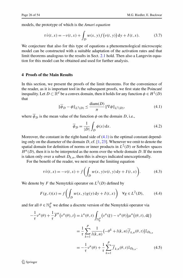
Page 26 of 54 M.G. Riedler, E. Buckwar
models, the prototype of which is the Amari equation
τ ν(t, x) = −ν(t, x) +∫
D
w(x, y)f(ν(t, y)
)dy + I (t, x). (3.7)
We conjecture that also for this type of equations a phenomenological microscopicmodel can be constructed with a suitable adaptation of the activation rates and thatlimit theorems analogous to the results in Sect. 2.1 hold. Then also a Langevin equa-tion for this model can be obtained and used for further analysis.
4 Proofs of the Main Results
In this section, we present the proofs of the limit theorems. For the convenience ofthe reader, as it is important tool in the subsequent proofs, we first state the Poincaréinequality. Let D ⊂ R
d be a convex domain, then it holds for any function φ ∈ H 1(D)
that
‖φD − φ‖L2(D) ≤ diam(D)
π‖∇φ‖L2(D), (4.1)
where φD is the mean value of the function φ on the domain D, i.e.,
φD = 1
|D|∫
D
φ(x)dx. (4.2)
Moreover, the constant in the right-hand side of (4.1) is the optimal constant depend-ing only on the diameter of the domain D, cf. [1, 23]. Whenever we omit to denote thespatial domain for definition of norms or inner products in L2(D) or Sobolev spacesHα(D), then it is to be interpreted as the norm over the whole domain D. If the normis taken only over a subset Dk,n, then this is always indicated unexceptionally.
For the benefit of the reader, we next repeat the limiting equation
τ ν(t, x) = −ν(t, x) + f
(∫D
w(x, y)ν(t, y)dy + I (t, x)
). (4.3)
We denote by F the Nemytzkii operator on L2(D) defined by
F(g, t)(x) = f
(∫D
w(x, y)g(y)dy + I (t, x)
)∀g ∈ L2(D), (4.4)
and for all θ ∈ NP0 we define a discrete version of the Nemytzkii operator via
−1
τνn(θ) + 1
τF
n(νn(θ), t
) = λn(θ, t)
∫N
P0
(νn(ξ) − νn(θ)
)μn((θ, t),dξ
)= 1
τ
P∑k=1
1
l(k, n)
(−θk + l(k, n)f k,n(θ, t))IDk,n
= −1
τνn(θ) + 1
τ
P∑k=1
f k,n(θ, t)IDk,n. (4.5)

Journal of Mathematical Neuroscience (2013) 3:1 Page 27 of 54
Note that τ−1(φ, νn(θ))L2 + τ−1(φ,Fn(νn(θ), t))L2 for φ ∈ L2(D) corresponds to
the generator of (Θnt , t)t≥0 applied to the function (θ, t) �→ (φ, νn(θ))L2 .
Finally, another useful property is that the means of the process’ components arebounded. For each k, n it holds that
EΘk,nt = EΘ
k,n0 + 1
τ
∫ t
0l(k, n)Ef k,n
(Yn
s
)− EΘk,ns ds
≤ EΘk,n0 + 1
τ
∫ t
0l(k, n)‖f ‖0 − EΘk,n
s ds,
see also (B.1). Therefore, it holds that EΘk,nt ≤ m
k,nt , where m
k,nt solves the deter-
ministic initial value problem
mk,nt = −1
τm
k,nt + 1
τl(k, n)‖f ‖0, m
k,n0 = EΘ
k,n0 ,
i.e.,
mk,nt = e−t/τ
(m0
k,n − l(k, n)‖f ‖0)+ l(k, n)‖f ‖0
≤ l(k, n)(1+ ‖f ‖0
) ∀t ≥ 0. (4.6)
Here, we also used the assumption EnΘ
k,n0 ≤ l(k, n) on the initial condition.
4.1 Proof of Theorem 2.1 (Law of Large Numbers)
In order to prove the law of large numbers, Theorem 2.1, we apply the law of largenumbers for Hilbert space valued PDMPs, see Theorem 4.1 in [27], to the sequence ofhomogeneous PDMPs (Y n
t )t≥0 = (Θnt , t)t≥0. For the application of this theorem, re-
call that the first, piecewise constant, vector-valued component of this process countsthe number of active neurons in each sub-population and the second, deterministiccomponent states time. The process (Y n
t )t≥0 is the usual ‘space-time process’, i.e.,homogeneous Markov process which is obtained via a state-space extension to ob-tain a homogeneous Markov process from the inhomogeneous process (Θn
t )t≥0. Thecontinuous component satisfies the simple ODE t = 1, t (0) = 0, and thus the fullprocess is a PDMP. In the terminology of [27], the sequence of coordinate functionson the different state spaces of the PDMPs (Y n
t )t≥0 into a common Hilbert space isgiven by the maps νn (2.7) with the common Hilbert space L2(D). Thus, in order toinfer convergence in probability (2.10) from Theorem 4.1 in [27], it is sufficient tovalidate the following conditions:
(LLN1) For fixed T > 0, it holds that
limn→∞ E
n
∫ T
0λn(Yn
t
)∫NP
∥∥νn(ξ) − νn(Θn
t
)∥∥2L2μ
n(Yn
t ,dξ)dt = 0. (4.7)
(LLN2) The Nemytzkii operator F satisfies a Lipschitz condition in L2(D) uni-formly with respect to t , t ≥ 0, i.e., there exists a constant L0 > 0 such

Page 28 of 54 M.G. Riedler, E. Buckwar
that∥∥F(g1, t)−F(g2, t)∥∥
L2 ≤ L0‖g1 −g2‖L2 ∀t ≥ 0, g1, g2 ∈ L2(D). (4.8)
(LLN3) For fixed T > 0, it holds that
limn→∞ E
n
∫ T
0
∥∥Fn(νnt , t)− F
(νnt , t)∥∥
L2 dt = 0. (4.9)
Note that the final condition of Theorem 4.1 in [27], i.e., the convergence of the initialconditions, is satisfied by assumption. For a discussion of these conditions, we referto [27] and proceed to their derivation for the present model in the subsequent parts(a) to (c).
(a) In order to prove condition (4.7), we write the integral with respect to the discreteprobability measure μn as a sum. This yields
Enλ(Yn
t
)∫NP
∥∥νn(ξ) − νn(Θn
t
)∥∥2L2μ
n(Yn
t ,dξ)
= 1
τ
P∑k=1
En 1
l(k, n)2
(Θ
k,nt + l(k, n)f k,n
(Yn
t
))|Dk,n|
≤ 1
τ
1+ 2‖f ‖0�−(n)
|D|, (4.10)
where we have used the upper bound (4.6) on the expectation EnΘ
k,nt and the
assumption on the initial conditions. Next, integrating over [0, T ] and employingthe assumption limn→∞ �−(n) = ∞ in (2.9) establishes condition (4.7).
(b) The Lipschitz condition (4.8) of the Nemytzkii operators is a straightforwardconsequence of the Lipschitz continuity (1.4) of the gain function f as∥∥F(g1, t) − F(g2, t)
∥∥2L2
=∫
D
∣∣∣∣f(∫D
w(x, y)g1(y)dy + I (x, t)
)
− f
(∫D
w(x, y)g2(y)dy + I (x, t)
)∣∣∣∣2 dx≤ L2
∫D
∣∣∣∣∫D
w(x, y)(g1(y) − g2(y)
)dy
∣∣∣∣2 dx≤ L2
∫D
∥∥w(x, ·)∥∥2L2‖g1 − g2‖2L2 dx
= L2‖w‖2L2×L2‖g1 − g2‖2L2 .
Therefore, (4.8) holds with Lipschitz constant L0 := L‖w‖L2×L2 .

Journal of Mathematical Neuroscience (2013) 3:1 Page 29 of 54
(c) Finally, we prove the convergence of the generators (4.9). To this end, we employthe characterisation of the norm in L2(D) by ‖η‖L2 = sup‖φ‖
L2=1 |(φ, η)L2 | forall η ∈ L2(D), and thus consider first the scalar product of elements φ ∈ L2(D)
with ‖φ‖L2 = 1 and the difference inside the norm in (4.9). On the one hand, weobtain using definition (4.5) that
(φ,F
n(νnt , t))
L2 =(
φ,
P∑k=1
f k,n
(Yn
t
)IDk,n
)L2
. (4.11)
Next, we apply the Nemytzkii operator F defined in (4.4) to νn(t) and take theinner product of the result with respect to φ to obtain on the other hand
(φ,F
(νnt , t))
L2 =(
φ,f
(P∑
k=1
Θk,nt
l(k, n)
∫Dk,n
w(·, y)dy + I (t, ·)))
L2
. (4.12)
Subtracting (4.12) from (4.11), we obtain the integrated difference(φ,F
n(νnt , t))
L2 − (φ,F(νnt , t))
L2
=∫
D
φ(x)
[P∑
k=1
f k,n
(Yn
t
)IDk,n
− f
(P∑
j=1
Θnj (t)
l(j, n)
∫Dj,n
w(x, y)dy + I (t, x)
)]dx
=P∑
k=1
∫Dk,n
φ(x)
[f
(P∑
j=1
Wn
kj
Θj,nt
l(j, n)+ I k,n(t)
)
− f
(P∑
j=1
Θj,nt
l(j, n)
∫Dj,n
w(x, y)dy + I (t, x)
)]dx.
We proceed to estimate the norm of the term in the right-hand side. We use theLipschitz condition (1.4) on f , the triangle inequality, and finally the Cauchy–Schwarz inequality on the resulting second term to obtain the estimate∣∣(φ,F
n(νnt , t))
L2 − (φ,F(νnt , t))
L2
∣∣≤ L
P∑k=1
∫Dk,n
∣∣φ(x)∣∣
×∣∣∣∣∣
P∑j=1
Θnj (t)
l(j, n)
(W
n
kj −∫
Dj,n
w(x, y)dy
)+ I k,n(t) − I (t, x)
∣∣∣∣∣dx

Page 30 of 54 M.G. Riedler, E. Buckwar
≤ L
P∑k=1
∫Dk,n
∣∣φ(x)∣∣∣∣∣∣∣
P∑j=1
Θnj (t)
l(j, n)
(W
n
kj −∫
Dj,n
w(x, y)dy
)∣∣∣∣∣dx︸ ︷︷ ︸(∗)
+ L
P∑k=1
‖φ‖L2(Dk,n)
∥∥I k,n(t) − I (t)∥∥
L2(Dk,n)︸ ︷︷ ︸(∗∗)
.
Here, the term in the right-hand side marked (∗∗) is further estimated using theCauchy–Schwarz inequality and the Poincaré inequality (4.1), which yields
(∗∗) ≤ δ+(n)
π
(P∑
k=1
∥∥∇I (t)∥∥2
L2(Dk,n)
)1/2
= δ+(n)
π
∥∥∇xI (t)∥∥
L2 . (4.13)
We now consider the term marked (∗). Inserting the definition of Wn
kj given in(2.4), the reordering of the summations and changing the order of integrationyields
(∗) =P∑
k=1
∫Dk,n
∣∣φ(x)∣∣
×∣∣∣∣∣
P∑j=1
Θj,nt
l(k, n)
(∫Dj,n
(1
|Dk,n|∫
Dk,n
w(z, y)dz
)− w(x,y)dy
)∣∣∣∣∣dx≤
P∑k=1
∫Dk,n
∣∣φ(x)∣∣
×P∑
j=1
Θj,nt
l(k, n)
∫Dj,n
∣∣∣∣( 1
|Dk,n|∫
Dk,n
w(z, y)dz
)− w(x,y)
∣∣∣∣dy dx=
P∑k=1
P∑j=1
Θj,nt
l(k, n)
×∫
Dj,n
[∫Dk,n
∣∣φ(x)∣∣∣∣∣∣( 1
|Dk,n|∫
Dk,n
w(z, y)dz
)− w(x,y)
∣∣∣∣dx]dy.
We next apply the Cauchy–Schwarz inequality to the integral inside the squarebrackets in the last term. Thus, we obtain the estimate
(∗) ≤P∑
j=1
∫Dj,n
P∑k=1
‖φ‖L2(Dk,n)
×[∫
Dk,n
∣∣∣∣( 1
|Dk,n|∫
Dk,n
w(z, y)dz
)− w(x,y)
∣∣∣∣2 dx]1/2 dy.

Journal of Mathematical Neuroscience (2013) 3:1 Page 31 of 54
Now the Poincaré inequality (4.1) is applied to the innermost integral inside thesquare brackets, which yields
(∗) ≤P∑
j=1
Θj,nt
l(k, n)
∫Dj,n
P∑k=1
‖φ‖L2(Dk,n)
diam(Dk,n)
π
∥∥∇xw(·, y)∥∥
L2(Dk,n)dy.
Finally, using once more the Cauchy–Schwarz inequality on the innermost sum-mation we obtain
(∗) ≤ δ+(n)
π
P∑j=1
Θj,nt
l(k, n)
∫Dj,n
∥∥∇xw(·, y)∥∥
L2 dy. (4.14)
Now, a combination of the estimates (4.13) and (4.14) on the terms (∗) and(∗∗) yields∣∣(φ,F
n(νnt , t))
L2 − (φ,F(νn(t), t
))L2
∣∣≤ δ+(n)
L
π
(P∑
j=1
Θj,nt
l(k, n)
∫Dj,n
∥∥∇xw(·, y)∥∥
L2 dy + ∥∥∇xI (t)∥∥
L2
).
Here, the right-hand side is independent of φ, hence taking the supremum overall φ with ‖φ‖L2 = 1 yields∥∥Fn(
νnt , t)− F
(νn(t), t
)∥∥L2
≤ δ+(n)L
π
(P∑
j=1
Θj,nt
l(k, n)
∫Dj,n
∥∥∇xw(·, y)∥∥
L2 dy + ∥∥∇xI (t)∥∥
L2
).
Finally, integrating over (0, T ) and taking the expectation on both sides results in
En
∫ T
0
∥∥Fn(νnt , t)− F
(νn(t), t
)∥∥L2 dt
≤ δ+(n)L
π
(√|D|T (1+ ‖f ‖0)‖∇xw‖L2×L2 + ‖∇xI‖L1((0,T ),L2)
).
(4.15)
Here, we have used (4.6) and a combination of the Cauchy–Schwarz and Poincaréinequality (4.1) in order to estimate
En
P∑j=1
Θj,nt
l(k, n)
∫Dj,n
∥∥∇xw(·, y)∥∥
L2 dy ≤ δ+(n)
√|D|(1+ ‖f ‖0)π
‖∇xw‖L2×L2 .
The upper bound in (4.15) is of order O(δ+(n)) and, therefore, converges to zerofor n → ∞ due to assumption (2.9). Hence, condition (4.9) is satisfied. The proofof the convergence in probability (2.10) is completed.

Page 32 of 54 M.G. Riedler, E. Buckwar
It is now easy to extend this result to the convergence in the r th mean. Firstof all, the convergence in probability (2.10) implies for all r ≥ 1 the convergencein probability of the random variables supt∈[0,T ] ‖νn
t − ν(t)‖rL2 to zero. As conver-
gence in the mean of real valued random variables is equivalent to convergence inprobability and uniform integrability it remains to prove the latter for the familiessupt∈[0,T ] ‖νn
t − ν(t)‖rL2 , n ∈ N.
We first consider the case r = 1, and establish a uniform bound on the second mo-ments E
n supt∈[0,T ] ‖νnt − ν(t)‖2
L2 . Then the de la Vallée–Poussin theorem, cf. App.,Proposition 2.2 in [15], implies that the random variables supt∈[0,T ] ‖νn
t − ν(t)‖L2 ,n ∈ N, are uniformly integrable.
Without loss of generality, we can assume that there exist5 Poisson processes(N
k,nt )t≥0 with rates Λk,n = l(k, n)(1+ ‖f ‖0)/τ , which dominate (Θ
k,nt − Θ
k,n0 )t≥0
pathwise. Then we obtain almost surely
∥∥νnt
∥∥2L2 ≤ 2
∥∥νn0
∥∥2L2 +2
P∑k=1
(Θk,nt − Θ
k,n0 )2
l(k, n)2|Dk,n| ≤ 2
∥∥νn0
∥∥2L2 +2
P∑k=1
(Nk,nT )2
l(k, n)2|Dk,n|.
Here, the right-hand side is independent of t ≤ T , and thus we obtain
En sup
t∈[0,T ]
∥∥νnt
∥∥2L2 ≤ 2E
n∥∥νn
0
∥∥2L2 + 2
P∑k=1
En(N
k,nT )2
l(k, n)2|Dk,n| ≤ 2E
n∥∥νn
0
∥∥2L2 + CT ,
where we have used that Nk,nT is Poisson distributed with rate T Λk,n, and thus
En(N
k,nT )2 = T Λk,n +T 2Λ2
k,n. Here, CT is some finite constant which depends on T
and the overall parameters of the model, i.e., τ , f , D, but is independent of k and n.Using this upper bound, the triangle inequality yields the estimate
En sup
t∈[0,T ]∥∥νn
t − ν(t)∥∥2
L2 ≤ 2CT
(E
n∥∥νn
0
∥∥2L2 + ‖ν‖2
C([0,T ],L2)+ 1).
Therefore, using the assumption supn∈N En‖νn
0‖2L2 < ∞ it holds that
supn∈N
En sup
t∈[0,T ]
∥∥νnt − ν(t)
∥∥2L2 < ∞.
The general case for r > 1 works analogously. Note that the r th moment of thePoisson distribution is proportional to the r th power of its rate. Hence, just as in thecase of r = 1, the term
En
(P∑
k=1
(Nk,nT )2
l(k, n)2|Dk,n|
)r
5The Poisson process jumps at a faster rate than the components of the Markov chain regardless of thetime and the state these are in. Furthermore, all jumps are upward. Hence, using a coupling argument asdiscussed in the proof of Theorem 4.3.5 in [16], we find that there exists a probability space supportingtwo processes with distributions equivalent to the Poisson process and the Markov chain component suchthat the Poisson process dominates the second process for all paths. Clearly, all moments dominate andthese inequalities are then valid for any probability spaces supporting these processes.

Journal of Mathematical Neuroscience (2013) 3:1 Page 33 of 54
can thus be bounded from above by some constant CT independent of k and n. Theproof of Theorem 2.1 is completed.
4.2 Proof of Corollary 2.1 (Corollary to the Law of Large Numbers)
For α = 0, the statement of the corollary coincides with the statement of Theorem 2.1,hence we consider α > 0. As in the proof of Theorem 2.1, we apply Theorem 4.1 in[27] to the PDMPs (Y n
t )t≥0, however, this time for the functions νn understood as tak-ing values in the Hilbert space H−α(D) instead of L2(D). Thus, we have to validateagain conditions (LLN1)–(LLN3) wherein the norm in L2(D) is always replaced bythe norm in H−α(D). The essential argument is sharpening the estimates in part (a)of the proof of Theorem 2.1 using optimal Sobolev embedding theorems such that theconditions (2.13) imply (LLN1). This we present in part (a) of the proof below. TheLipschitz condition (LLN2) of the Nemytzkii operator F in the spaces H−α is estab-lished in part (b). Finally, as the condition δ+(n) → ∞ remains as in Theorem 2.1,the condition (LLN3) follows immediately from the proof of Theorem 2.1 due to thecontinuous embedding of L2(D) into H−α(D).
(a) In the case α = 0, i.e., Hα(D) = L2(D), we used in (4.10) that ‖IDk,n‖2L2 =
|Dk,n|. For general α > 0, we use the representation
‖IDk,n‖H−α = sup
‖φ‖Hα
∣∣(φ, IDk,n)L2
∣∣.In order to estimate the terms inside the supremum in the right-hand side, we useHölder’s inequality and the Sobolev embedding theorem, i.e.,Hα(D) ↪→ L∞(D)
for α > d/2 and Hα(D) ↪→ Lr(D) with r = d/(d/2 − α) for 0 < α < d/2, seeTheorem 7.34 and Corollary 7.17 in [2]. Thus, we obtain
‖IDk,n‖H−α ≤
{Kd/(d/2−α)‖IDk,n
‖L2d/(d+2α) if 0 < α < d/2,
K∞‖IDk,n‖L1 if d/2< α,
where the constants K are the constants arising from the continuous embeddingsof the Sobolev spaces into the Lebesgue spaces. Evaluating the norms in theright-hand side, and further estimating using the maximal Lebesgue measure ofthe elements of the partition yields
‖IDk,n‖2H−α ≤
{K2
d/(d/2−α)|Dk,n|v+(n)2α/d if 0 < α < d/2,
K2∞|Dk,n|v+(n) if d/2< α.
Note that the upper bounds are consistent with the condition in Theorem 2.1for α = 0. Finally, as Hd/2(D) ↪→ H(d/2−ε)(D) for all small ε, the result forα = d/2 follows from the result above as
‖IDk,n‖H−d/2 ≤ sup
‖φ‖H2α
(‖φ‖Ld/ε‖IDk,n‖Ld/(d−ε)
)≤ C‖IDk,n‖Ld/(d−ε)

Page 34 of 54 M.G. Riedler, E. Buckwar
where C is the constant resulting from the continuous embedding of Hd/2(D)
into Hd/2−ε(D). Thus, we obtain for all ε > 0 the estimate
‖IDk,n‖2H−d/2 ≤ C2|Dk,n|v+(n)(d−2ε)/d .
(b) Next, we have to establish that the Nemytzkii operator F on L2(D) is also Lip-schitz continuous with respect to the norms ‖ · ‖H−α , α ≥ 0, i.e., for all α ≥ 0there exists a constant L−α such that∥∥F(g1, t) − F(g2, t)
∥∥H−α ≤ L−α‖g1 − g2‖H−α ∀t ≥ 0, g1, g2 ∈ L2(D).
(4.16)We obtain due to the Lipschitz continuity of f , which implies absolute continuityof f , that∣∣∣∣∫
D
φ(x)(F(g1, t)(x) − F(g2, t)(x)
)dx
∣∣∣∣= ∣∣∣∣∫D
φ(x)
∫ z2(t,x)
z1(t,x)
f ′(z)dzdx∣∣∣∣,
where
z1(t, x) =∫
D
w(x, y)g1(y)dy + I (t, x),
z2(t, x) =∫
D
w(x, y)g2(y)dy + I (t, x).
Applying Hölder’s inequality and the essential boundedness of the derivative f ′,we obtain the estimate∣∣∣∣∫
D
φ(x)(F(g1, t)(x) − F(g2, t)(x)
)dx
∣∣∣∣≤ ‖φ‖Lp
(∫D
∣∣∣∣∫ z2(t,x)
z1(t,x)
f ′(z)dz∣∣∣∣q dx)1/q
≤ ‖φ‖Lp
(∫D
∣∣∥∥f ′∥∥L∞(z1(t, x) − z2(t, x)
)∣∣q dx)1/q= ‖φ‖Lp‖f ′‖L∞
(∫D
∣∣∣∣∫D
w(x, y)(g1(y) − g1(y)
)dy
∣∣∣∣q dx)1/q .
Next, as by assumption w(x, ·) ∈ Hα(D), we obtain(∫D
∣∣∣∣∫D
w(x, y)(g1(y) − g1(y)
)dy
∣∣∣∣q dx)1/q=(∫
D
∥∥w(x, ·)∥∥q
Hα
∣∣⟨w(x, ·)/∥∥w(x, ·)∥∥Hα , g1 − g2
⟩Hα
∣∣q)1/q≤ ‖w‖Lq×Hα‖g1 − g2‖H−α .

Journal of Mathematical Neuroscience (2013) 3:1 Page 35 of 54
Overall, this yields the estimate∣∣⟨φ,F (g1, t) − F(g2, t)⟩H−α
∣∣≤ ‖φ‖Lp
∥∥f ′∥∥L∞‖w‖Lq×Hα‖g1 − g2‖H−α .
Hence, taking the supremum on both sides of this inequality over all ‖φ‖Hα = 1,we obtain the Lipschitz condition (4.16) with L−α := LKα‖w‖Lq×Hα , where Kα
is the constant resulting from the continuous embedding of Hα(D) into Lp(D)
and the Lipschitz constant L of f satisfies L ≥ ‖f ′‖L∞ .
4.3 Proof of Theorem 2.2 (Infinite Time Convergence)
(a) We first present an alternative representation for the jump processes (Θnt )t≥0 and
the solution ν of the Wilson–Cowan equation (1.3). Using the generator of thePDMP (Θn
t , t)t≥0, we obtain that the components Θk,n satisfy
Θk,nt = Θ
k,n0 +
∫ t
0λn(Θn
s , s)∫
Np
(ξk − Θk,n
s
)μn(Θn
s , s;dξ)ds + Mk,nt
= Θk,n0 +
∫ t
0
(−1
τΘk,n
s + 1
τl(k, n)f k,n
(Θn
s , s))
ds + Mk,nt , (4.17)
where (Mk,nt )t≥0 is a square-integrable càdlàg martingale given by
Mk,nt := Θ
k,nt −Θ
k,n0 −
∫ t
0λn(Θn
s , s) ∫
Np
(ξk −Θk,n
s
)μn(Θn
s , s;dξ)ds. (4.18)
As the jump process is regular, this martingale is almost surely of finite varia-tion and it could also be written in terms of a stochastic integral with respect tothe associated martingale measure of the PDMP [16]. Next, interpreting Θk,n asthe solution of the stochastic evolution equation (4.17) driven by the martingaleMk,n, it follows from the variation of constants formula that it satisfies
Θk,nt = e−t/τΘ
k,n0 + 1
τl(k, n)
∫ t
0e−(t−s)/τ f k,n
(Θn
s , s)ds
+∫ t
0e−(t−s)/τ dMk,n
s . (4.19)
This formula can also be easily verified path-by-path by inserting (4.19) into(4.17) and using integration by parts. Note that here the stochastic integral withrespect to the martingale is just a Riemann–Stieltjes integral as the martingale isof finite variation. For the sake of completeness, we briefly sketch the arguments.Thus, inserting (4.19) into (4.17) yields
Θk,nt = Θ
k,n0 − 1
τ
∫ t
0e−s/τΘ
k,n0 ds︸ ︷︷ ︸
(∗)
− 1
τl(k, n)

Page 36 of 54 M.G. Riedler, E. Buckwar
×(1
τ
∫ t
0
∫ s
0e−(s−r)/τ f k,n
(Θn
r , r)dr ds −
∫ t
0f k,n
(Θn
s , s)ds︸ ︷︷ ︸
(∗∗)
)
−1
τ
∫ t
0
∫ s
0e−(s−r)/τ dMk,n
r ds + Mk,nt︸ ︷︷ ︸
(∗∗∗)
.
Considering the three terms marked (∗)–(∗ ∗ ∗) separately, we show that thisright-hand side equals (4.19). For the first term (∗) simply evaluating the integralyields
Θk,n0 − 1
τ
∫0t
e−s/τΘk,n0 ds = Θ
kn
0 − 1
τ
(α−1e−t/τ − τ
)Θ
k,n0 = e−t/τΘ
k,n0 ,
which gives the first term in the right-hand side of (4.19). Next, we simplify theterm (∗∗) employing integration by parts to the first term in (∗∗), which yields
1
τ
∫ t
0
∫ s
0e−(s−r)/τ f k,n
(Θn
r , r)dr ds
= 1
τ
∫ t
0e(t−s)/τ
∫ s
0e−(t−r)/τ f k,n
(Θn
r , r)dr ds
= 1
τ
(−τe(t−s)/τ
∫ s
0e−(t−r)/τ f k,n
(Θn
r , r)dr
)∣∣∣∣t0
− 1
τ
∫ t
0(−τ)e(t−s)τ e−(t−s)/τ f k,n
(Θn
s , s)ds
= −∫ t
0e−(t−s)/τ f k,n
(Θn
s , s)ds +
∫ t
0f k,n
(Θn
s , s)ds.
Thus, we obtain subtracting from this right-hand side the second term in (∗∗)
that
(∗∗) = −∫ t
0e−(t−s)/τ f k,n
(Θn
s , s)ds.
This term is just the second term in the right-hand side of (4.19). It remains toconsider the term marked (∗ ∗ ∗). We have already stated that the stochastic inte-gral with respect to the martingale (4.18) is defined path-by-path as a Riemann–Stieltjes integral, and thus satisfies
−1
τ
∫ s
0e−(s−r)/τ dMk,n
s
= −1
τ
∑τnj ≤s
e−(s−τnj )/τ (
Θk,n
τnj
− Θk,n
τnj−
)

Journal of Mathematical Neuroscience (2013) 3:1 Page 37 of 54
+ 1
τ
∫ s
0e−(s−r)/τ λn
(Θn
r , r)
×∫
NP0
(ξk − Θk,n
r
)μn((
Θnr , r),dξ)ds, (4.20)
where τnj denotes the j th jump time of the nth PDMP. Integrating the sum in this
right-hand side over (0, t) yields
−1
τ
∫ t
0
∑τnj ≤s
e−(s−τnj )/τ (
Θk,n
τnj
− Θk,n
τnj−
)ds
=∑τnj ≤t
e−(t−τnj )/τ (
Θk,n
τnj
− Θk,n
τnj−
)− ∑τnj ≤t
(Θ
k,n
τnj
− Θk,n
τnj−
)=∑τnj ≤t
e−(t−τnj )/τ (
Θk,n
τnj
− Θk,n
τnj−
)− (Θk,nt − Θ
k,n0
).
Next, we apply integration by parts to the integral over (0, t) of the second termabove analogously to the application to term (∗∗), and obtain
1
τ
∫ t
0
∫ s
0e−α(s−r)λn
(Θn
r , r)∫
NP0
(ξk − Θk,n
r
)μn((
Θnr , r),dξ)dr ds
= −∫ t
0e−(t−s)/τ λn
(Θn
s , s)∫
NP0
(ξk − Θk,n
s
)μn((
Θns , s),dξ)ds
+∫ t
0λn(Θn
s , s) ∫
NP0
(ξk − Θk,n
s
)μn((
Θns , s),dξ)ds.
Hence, overall these considerations show that
(∗ ∗ ∗) =∫ t
0e−(t−s)/τ dMk,n
s
and we obtain the final, third term in the right-hand side of (4.19). This completesthe proof that (4.19) solves Eq. (4.17).
Further, we obtain from the variation of constants formula for Θk,nt also a
representation for the stochastic mean activity νn by inserting (4.19) into its def-inition (2.7). This gives
νnt = e−t/τ νn
0 + 1
τ
P∑k=1
∫ t
0e−(t−s)/τ f k,n
(Θn
s , s)dsIDk,n
+P∑
k=1
1
l(k, n)
∫ t
0e−(t−s)/τ dMk,n
s IDk,n

Page 38 of 54 M.G. Riedler, E. Buckwar
= e−t/τ νn0 + 1
τ
∫ t
0e−(t−s)/τF
n(νns , s)ds
+P∑
k=1
1
l(k, n)
∫ t
0e−(t−s)/τ dMk,n
s IDk,n. (4.21)
Finally, in order to compare stochastic and deterministic solutions we use thatthe solution of the Wilson–Cowan equation can also be given via the variation ofconstants formula, i.e., it holds that for all t ≥ 0
ν(t) = e−t/τ ν(0) + 1
τ
∫ t
0e−(t−s)/τF
(ν(s), s
)ds. (4.22)
Thus, subtracting (4.22) from (4.21), and taking the expectation of the norm inH−α(D) yields the estimate
En∥∥ν(t) − νn
t
∥∥H−α
= e−t/τE
n∥∥ν(0) − νn
0
∥∥H−α
+ 1
τ
∫ t
0e−(t−s)/τ
En∥∥F (ν(s), s
)− Fn(
νns , s)∥∥
H−α
+ En
∥∥∥∥∥P∑
k=1
1
l(k, n)
∫ t
0e−(t−s)/τ dMk,n
s IDk,n
∥∥∥∥∥H−α
. (4.23)
We deal with the terms in the right-hand side of (4.23) separately in the followingsuch that we can apply Gronwall’s inequality. Note that the term containing theinitial condition vanishes due to the assumptions of the theorem. We start withthe stochastic integrals in the subsequent part (b) of the proof.
(b) As due to Jensen’s inequality E|Y | ≤ √E|Y |2, it makes sense to calculate thesecond moment of the stochastic integral in the right-hand side. For the norm inH−α(D), we use ‖φ‖2
H−α = (φ,φ)H−α , and thus obtain using the linearity of theinner product∥∥∥∥∥
P∑k=1
1
l(k, n)
∫ t
0e−(t−s)/τ dMk,n
s︸ ︷︷ ︸=:βk,n
t
IDk,n
∥∥∥∥∥2
H−α
=P∑
k=1
|βk,n|2l(k, n)2
‖IDk,n‖2H−α +
P∑k,j=1k �=j
βk,nβj,n
l(k, n)l(j, n)(IDk,n
, IDj,n)H−α .
We next consider the individual expectations of the random terms |βk,n|2 andβk,nβj,n in the right-hand side. We have already stated that the stochastic inte-

Journal of Mathematical Neuroscience (2013) 3:1 Page 39 of 54
gral with respect to the martingale (4.18) is defined path-by-path as a Riemann–Stieltjes integral (see (4.20)) and, moreover, (4.20) implies that the stochasticconvolution integral can be written as a stochastic integral with respect to thefundamental martingale measure Mn associated with the PDMP (Θn
t , t)t≥0 (see[16]), i.e.,∫ t
0e−(t−s)/τ dMk,n
s =∫
[0,t]×NP0
e−(t−s)/τ(ξk − Θ
k,ns−)Mn(ds,dξ)
with predictable integrand
(ξ, s,ω) �→ e−(t−s)/τ(ξk − Θ
k,ns− (ω)
).
Then we obtain due to the Itô-isometry following from Proposition 4.6.2 in [16]using (4.6) that
En
∣∣∣∣∫ t
0e−(t−s)/τ dMk,n
s
∣∣∣∣2= E
n
∫ t
0λn(Yn
s
)∫N
P0
e−2(t−s)/τ(ξk − Θk,n
s
)2μn(Yn
s ,dξ)ds
≤ En
∫ t
0e−2(t−s)/τ
(1
τΘk,n
s + 1
τl(k, n)f k,n
(Yn
s
))ds
≤ 1
τ
(E
nΘk,n0 + 2l(k, n)‖f ‖0
)∫ t
0e−2(t−s)/τ ds.
It remains to consider the product βk,nt β
j,nt for which we obtain due to the inte-
gration by parts formula
βk,nt β
j,nt =
∫ t
0β
k,ns− dβj,n
s +∫ t
0β
j,ns− dβk,n
s + [βk,n, βj,n]t, (4.24)
where the square brackets denote the quadratic variation process. The expectationof each of the terms in the right-hand side vanishes: The first two are stochasticintegrals with respect to martingales, hence martingales themselves which areidentical to zero at the origin. Furthermore, as both martingales are càdlàg withpaths of finite variation on compacts, hence quadratic pure jump martingales, weobtain for the quadratic variation process[
βk,n, βj,n]t=∑s≤t
(βk,n
s − βk,ns−)(
βj,ns − β
j,ns−).
However, as all jump times of the two martingales a.s. differ it follows that[βk,n, βj,n]t = 0.

Page 40 of 54 M.G. Riedler, E. Buckwar
Thus, overall we have established that
En
∥∥∥∥∥P∑
k=1
1
l(k, n)
∫ t
0e−(t−s)/τ dMk,n
s IDk,n
∥∥∥∥∥2
H−α
= 1
2
P∑k=1
1+ 2‖f ‖0l(k, n)
‖IDk,n‖2H−α , (4.25)
where 1/2 is an upper bound for 1τ
∫ t
0 e−2(t−s)/τ ds independent of t . Estimat-
ing the norm ‖IDk,n‖2H−α just as in the proof of Corollary 2.1, we finally obtain
that
En
∥∥∥∥∥P∑
k=1
1
l(k, n)
∫ t
0e−(t−s)/τ dMk,n
s IDk,n
∥∥∥∥∥H−α
≤ 1
4
((1+2‖f ‖0
)|D|v+(n)r
�−(n)
)1/2,
with r = 2α/d for 0 ≤ α ≤ d/2, r = 1 − ε for α = d/2 and r = 1 for α >
d/2.(c) We next estimate the term∫ t
0e−(t−s)/τ
En∥∥F (ν(s), s
)− Fn(
νns , s)∥∥
H−α
in (4.23). From part (b) of the proof of Theorem 2.1 in Sect. 4.1, it followsthat
En∥∥F (νn
t , t)− F
n(νnt , t)∥∥
H−α
≤ δ+(n)K−αL
π
(√|D|(1+ ‖f ‖0)‖∇xw‖L2×L2 + ∥∥∇xI (t)
∥∥L2
), (4.26)
where F is the Nemytzkii operator defined in (4.4) and K−α is a constantresulting from the continuous embedding of L2(D) into H−α(D). Here, theright-hand side can be further estimated independently of t ≥ 0 using the as-sumption that ‖∇xI (t)‖L2 is uniformly bounded in t ≥ 0. Furthermore, wehave shown in Sect. 4.2 in the proof of Corollary 2.1, that under the ap-propriate assumptions the Nemytzkii operator F is Lipschitz continuous onH−α(D), α ≥ 0, with Lipschitz constant L−α > 0 independent of t ≥ 0,i.e.,∥∥F(g1, t) − F(g2, t)
∥∥H−α ≤ L−α‖g1 − g2‖H−α ∀g1, g2 ∈ L2(D). (4.27)
A combination of the triangle inequality and the estimates (4.26) and (4.27)yields ∫ t
0e−(t−s)/τ
En∥∥F (ν(s), s
)− Fn(
νns , s)∥∥
H−α
≤ L−α
∫ t
0e−(t−s/τ)
En∥∥ν(s) − νn
s
∥∥H−α ds + O
(δ+(n)
).

Journal of Mathematical Neuroscience (2013) 3:1 Page 41 of 54
Overall, it thus follows from (4.23) that
En∥∥ν(t) − νn
t
∥∥H−α ≤ E
n∥∥ν(0) − νn
0
∥∥H−α
+ L−α
τ
∫ t
0e−(t−s/τ)
En∥∥ν(s) − νn
s
∥∥H−α ds
+ O(
δ+(n) +√
v+(n)r
�−(n)
).
Then an application of Gronwall’s inequality yields
En∥∥ν(t) − νn
t
∥∥H−α ≤
(E
n∥∥ν(0) − νn
0
∥∥H−α + O
(δ+(n) +
√v+(n)r
�−(n)
))
× exp
(L−α
τ
∫ t
0e−(t−s)/τ ds
)
≤(
En∥∥ν(0) − νn
0
∥∥H−α + O
(δ+(n) +
√v+(n)r
�−(n)
))eL−α .
By assumptions of the theorem, the term in the right-hand side converges to zerofor n → ∞. As this convergence is uniform in t , it holds that
limn→∞ sup
t≥0E
n∥∥ν(t) − νn
t
∥∥H−α = 0. (4.28)
4.4 Proof of Theorem 2.3 (Martingale Central Limit Theorem)
In order to prove the martingale central limit theorem, we employ the general martin-gale central limit theorem (Theorem 5.1 in [27]) for the Hilbert space H−α(D), i.e.,the dual of the Sobolev space Hα(D), for α > d . To apply this theorem, it suffices toprove the following conditions. Subsequently we use ρn =√�−(n)/v+(n) to denotethe re-scaling sequence and use the notation
⟨Gn(t)φ,φ
⟩Hα = λ
(Yn
t
)∫N
P0
⟨νn(ξ) − νn
(Θn
t
), φ⟩2Hαμ
n(Yn
t ,dξ)
(4.29)
which corresponds to the quadratic variation of the martingales (Mnt )t≥0, see [27] for
a discussion.
(CLT1) For all t > 0, it holds that
supn∈N
ρnEn
∫ t
0
[λn(Yn
s
)∫NP
∥∥νn(ξ) − νn(Θn
s
)∥∥2H−αμ
n(Yn
s ,dξ)ds
]< ∞, (4.30)
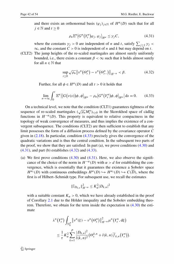
Page 42 of 54 M.G. Riedler, E. Buckwar
and there exists an orthonormal basis (ϕj )j∈N of Hα(D) such that for allj ∈ N and t ≥ 0
ρnEn⟨Gn(Yn
t
)ϕj ,ϕj
⟩Hα ≤ γjC, (4.31)
where the constants γj > 0 are independent of n and t , satisfy∑
j≥1 γj <
∞, and the constant C > 0 is independent of n and k but may depend on t .(CLT2) The jump heights of the re-scaled martingales are almost surely uniformly
bounded, i.e., there exists a constant β < ∞ such that it holds almost surelyfor all n ∈ N that
supt≥0
√ρn
∥∥νn(Θn
t
)− νn(Θn
t−)∥∥
H−α < β. (4.32)
Further, for all φ ∈ Hα(D) and all t > 0 it holds that
limn→∞
∫ t
0E
n∣∣⟨G(ν(s)
)φ,φ
⟩Hα − ρn
⟨Gn(Yn
s
)φ,φ
⟩Hα
∣∣ds = 0. (4.33)
On a technical level, we note that the condition (CLT1) guarantees tightness of thesequence of re-scaled martingales (
√ρnM
nt )t≥0 in the Skorokhod space of càdlàg
functions in H−α(D). This property is equivalent to relative compactness in thetopology of weak convergence of measures, and thus implies the existence of a con-vergent subsequence. The conditions (CLT2) are then sufficient to establish that anylimit possesses the form of a diffusion process defined by the covariance operator C
given in (2.18). In particular, condition (4.33) precisely gives the convergence of thequadratic variations and is thus the central condition. In the subsequent two parts ofthe proof, we show that they are satisfied: In part (a), we prove conditions (4.30) and(4.31), and part (b) establishes (4.32) and (4.33).
(a) We first prove conditions (4.30) and (4.31). Here, we also observe the signifi-cance of the choice of the norm in H−α(D) with α > d for establishing the con-vergence, which is essentially that it guarantees the existence a Sobolev spaceHα1(D) with continuous embeddings Hα(D) ↪→ Hα1(D) ↪→ C(D), where thefirst is of Hilbert–Schmidt type. For subsequent use, we recall the estimates
‖IDk,n‖2H−α ≤ K2
α|Dk,n|2
with a suitable constant Kα > 0, which we have already established in the proofof Corollary 2.1 due to the Hölder inequality and the Sobolev embedding theo-rem. Therefore, we obtain for the term inside the expectation in (4.30) the esti-mate
λn(Yn
s
)∫N
P0
∥∥νn(ξ) − νn(Θn
s
)∥∥2H−αμ
n(Yn
s ,dξ)
≤ 1
τK2
α
P∑k=1
|Dk,n|2l(k, n)2
(Θk,n
s + l(k, n)f k,n
(Yn
s
)).

Journal of Mathematical Neuroscience (2013) 3:1 Page 43 of 54
Next taking the expectation, using the bound (4.6) on EnΘ
k,ns and integrating
over [0, t] we obtain the estimate∫ t
0E
n
[λn(Yn
s
)∫N
P0
∥∥νn(ξ) − νn(Θn
s
)∥∥2H−αμ
n(Yn
s ,dξ)]
ds
≤ t
τK2
α
(1+ 2‖f ‖0
)v+(n)
�−(n).
Multiplying both sides with ρn = �−(n)/v+(n), we find that condition (4.30) issatisfied.
We proceed to condition (4.31) and first of all expand the integrand to obtain
⟨Gn(Yn
s
)ϕj ,ϕj
⟩Hα = λn
(Yn
s
)∫N
P0
⟨νn(ξ) − νn
(Θn
s
), φj
⟩2H−αμ
n(Yn
s ,dξ)
= 1
τ
P∑k=1
1
l(k, n)2
(Θk,n
s + l(k, n)f k,n
(Yn
s
))〈IDk,n, ϕj 〉2Hα .
We next estimate the term 〈IDk,n, ϕ〉2Hα . Here, we use the fact that for a function in
L2(D) its application as an element of the dual H−α(D) as well as H−α1(D) forany α1 with 0 ≤ α1 < α coincide. We choose α1 such that d/2 < α1 < α − d/2and obtain
〈IDk,n, ϕ〉2Hα ≤ ‖IDk,n
‖2H−α1‖ϕj‖2Hα1 ≤ K2
α1|Dk,n|2‖ϕj‖2Hα1 ,
where Kα1 is the constant resulting from the Sobolev embedding theorem. Next,taking the expectation, estimating the expectation terms as before and multiply-ing by ρn yields
ρnEn⟨Gn(Yn
t
)ϕj ,ϕj
⟩Hα ≤ 1
τK2
α1
(1+ ‖f ‖0
)‖ϕj‖2Hα1 .
We chose the constants in (4.31) as C := K2α1
(1+ ‖f ‖0)/τ and γj := ‖ϕj‖2Hα1 .Finally, as due to Maurin’s theorem the embedding of the space Hα(D) intoHα1(D) is of Hilbert–Schmidt type, cf. footnote 3 on page 16, it holds that∑
j≥1 ‖ϕj‖2Hα1 < ∞. Condition (4.31) is satisfied.(b) The estimates in part (a) further show that the jump sizes are almost surely uni-
formly bounded as
supt≥0
√ρn
∥∥νn(Θn
t
)− νn(Θn
t−)∥∥
H−α ≤ Kα
√v+(n)
�−(n).
Here, the upperbound in the right-hand side converges to zero for n → ∞, andthus the left-hand side is bounded over all n ∈ N. Therefore, condition (4.32)holds and we are left to prove the convergence of the quadratic variation (4.33).
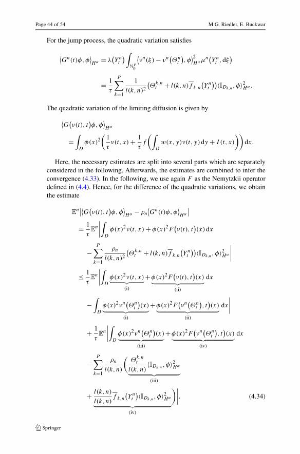
Page 44 of 54 M.G. Riedler, E. Buckwar
For the jump process, the quadratic variation satisfies
⟨Gn(t)φ,φ
⟩Hα = λ
(Yn
t
)∫N
P0
⟨νn(ξ) − νn
(Θn
t
), φ⟩2Hαμ
n(Yn
t ,dξ)
= 1
τ
P∑k=1
1
l(k, n)2
(Θ
k,nt + l(k, n)f k,n
(Yn
t
))〈IDk,n, φ〉2Hα .
The quadratic variation of the limiting diffusion is given by⟨G(ν(t), t
)φ,φ
⟩Hα
=∫
D
φ(x)2(1
τν(t, x) + 1
τf
(∫D
w(x, y)ν(t, y)dy + I (t, x)
))dx.
Here, the necessary estimates are split into several parts which are separatelyconsidered in the following. Afterwards, the estimates are combined to infer theconvergence (4.33). In the following, we use again F as the Nemytzkii operatordefined in (4.4). Hence, for the difference of the quadratic variations, we obtainthe estimate
En∣∣⟨G(ν(t), t
)φ,φ
⟩Hα − ρn
⟨Gn(t)φ,φ
⟩Hα
∣∣= 1
τE
n
∣∣∣∣∫D
φ(x)2ν(t, x) + φ(x)2F(ν(t), t
)(x)dx
−P∑
k=1
ρn
l(k, n)2
(Θ
k,nt + l(k, n)f k,n
(Yn
t
))〈IDk,n, φ〉2Hα
∣∣∣∣≤ 1
τE
n
∣∣∣∣∫D
φ(x)2ν(t, x)︸ ︷︷ ︸(i)
+φ(x)2F(ν(t), t
)(x)︸ ︷︷ ︸
(ii)
dx
−∫
D
φ(x)2νn(Θn
t
)(x)︸ ︷︷ ︸
(i)
+φ(x)2F(νn(Θn
t
), t)(x)︸ ︷︷ ︸
(ii)
dx
∣∣∣∣+ 1
τE
n
∣∣∣∣∫D
φ(x)2νn(Θn
t
)(x)︸ ︷︷ ︸
(iii)
+φ(x)2F(νn(Θn
t
), t)(x)︸ ︷︷ ︸
(iv)
dx
−P∑
k=1
ρn
l(k, n)
(Θ
k,nt
l(k, n)〈IDk,n
, φ〉2Hα︸ ︷︷ ︸(iii)
+ l(k, n)
l(k, n)f k,n
(Yn
t
)〈IDk,n, φ〉2Hα︸ ︷︷ ︸
(iv)
)∣∣∣∣. (4.34)
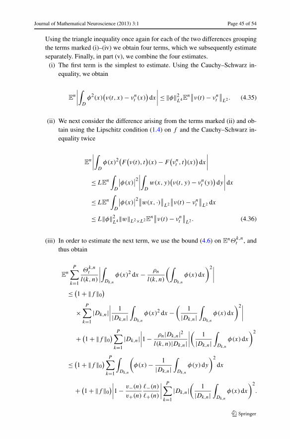
Journal of Mathematical Neuroscience (2013) 3:1 Page 45 of 54
Using the triangle inequality once again for each of the two differences groupingthe terms marked (i)–(iv) we obtain four terms, which we subsequently estimateseparately. Finally, in part (v), we combine the four estimates.(i) The first term is the simplest to estimate. Using the Cauchy–Schwarz in-
equality, we obtain
En
∣∣∣∣∫D
φ2(x)(ν(t, x) − νn
t (x))dx
∣∣∣∣≤ ‖φ‖2L4E
n∥∥ν(t) − νn
t
∥∥L2 . (4.35)
(ii) We next consider the difference arising from the terms marked (ii) and ob-tain using the Lipschitz condition (1.4) on f and the Cauchy–Schwarz in-equality twice
En
∣∣∣∣∫D
φ(x)2(F(ν(t), t
)(x) − F
(νnt , t)(x))dx
∣∣∣∣≤ LE
n
∫D
∣∣φ(x)∣∣2∣∣∣∣∫
D
w(x, y)(ν(t, y) − νn
t (y))dy
∣∣∣∣dx≤ LE
n
∫D
∣∣φ(x)∣∣2∥∥w(x, ·)∥∥
L2
∥∥ν(t) − νnt
∥∥L2 dx
≤ L‖φ‖2L4‖w‖L2×L2E
n∥∥ν(t) − νn
t
∥∥L2 . (4.36)
(iii) In order to estimate the next term, we use the bound (4.6) on EnΘ
k,nt , and
thus obtain
En
P∑k=1
Θk,nt
l(k, n)
∣∣∣∣∫Dk,n
φ(x)2 dx − ρn
l(k, n)
(∫Dk,n
φ(x)dx
)2∣∣∣∣≤ (1+ ‖f ‖0
)×
P∑k=1
|Dk,n|∣∣∣∣ 1
|Dk,n|∫
Dk,n
φ(x)2 dx −(
1
|Dk,n|∫
Dk,n
φ(x)dx
)2∣∣∣∣+ (1+ ‖f ‖0
) P∑k=1
|Dk,n|∣∣∣∣1− ρn|Dk,n|2
l(k, n)|Dk,n|∣∣∣∣( 1
|Dk,n|∫
Dk,n
φ(x)dx
)2
≤ (1+ ‖f ‖0) P∑
k=1
∫Dk,n
(φ(x) − 1
|Dk,n|∫
Dk,n
φ(y)dy
)2dx
+ (1+ ‖f ‖0)∣∣∣∣1− v−(n)
v+(n)
�−(n)
�+(n)
∣∣∣∣ P∑k=1
|Dk,n|(
1
|Dk,n|∫
Dk,n
φ(x)dx
)2.

Page 46 of 54 M.G. Riedler, E. Buckwar
Then the estimate is completed applying the Poincaré inequality (4.1) to thefirst term, that is, estimating
P∑k=1
∫Dk,n
(φ(x) − 1
|Dk,n|∫
Dk,n
φ(y)dy
)2dx ≤ diam(Dk,n)
2
π2‖∇φ‖2
L2,
and the observation that the second term is proportional to ‖φn‖2L2 , which
is the piecewise constant approximation to φ based on the partition Dn;see (4.2). Therefore, we overall obtain an upper bound for the differenceconstituted by the terms (iii) in (4.34) by
En
∣∣∣∣∫D
φ(x)2νnt (x)dx − ρn
P∑k=1
Θk,nt
l(k, n)2〈IDk,n
, φ〉2Hα
∣∣∣∣≤ δ+(n)2
1+ ‖f ‖0π2
‖φ‖2H 1 + (1+ ‖f ‖0
)R(n). (4.37)
In the last term,
R(n) :=∣∣∣∣1− v−(n)
v+(n)
�−(n)
�+(n)
∣∣∣∣∥∥φn∥∥2L2
converges to zero for n → ∞ by assumption (2.19) and as the sequence‖φn‖L2 is bounded as it converges to ‖φ‖L2 for n → ∞.
(iv) Finally, we consider the difference
En
∣∣∣∣∫D
φ(x)2F(νnt , t)(x)dx − ρn
P∑k=1
l(k, n)
l(k, n)2f k,n
(Yn
t
)〈IDk,n, φ〉2Hα
∣∣∣∣≤ E
n
P∑k=1
∣∣∣∣∫Dk,n
φ(x)2F(νnt , t)(x)dx − ρn
l(k, n)f k,n
(Yn
t
)〈φ, IDk,n〉2Hα
∣∣∣∣.We continue estimating the difference in each summand in the final right-hand side and obtain using the triangle inequality for the term inside theexpectation
En
P∑k=1
∣∣∣∣∫Dk,n
φ(x)2F(νnt , t)(x)dx − ρn
l(k, n)f k,n
(Yn
t
)〈IDk,n, φ〉2Hα
∣∣∣∣≤ E
n
P∑k=1
∣∣∣∣∫Dk,n
φ(x)2(F(νnt , t)(x) − f k,n
(Yn
t
))dx
∣∣∣∣︸ ︷︷ ︸(∗)
+ En
P∑k=1
∣∣∣∣f k,n
(Yn
t
)(∫Dk,n
φ(x)2 dx − ρn
l(k, n)〈IDk,n
, φ〉2Hα
)∣∣∣∣︸ ︷︷ ︸(∗∗)
.

Journal of Mathematical Neuroscience (2013) 3:1 Page 47 of 54
We start with the first term and observe that it possesses the same structureas the term estimated in part (c) of the proof of Theorem 2.1 with the onlydifference that here the function φ in the integrand is squared. Therefore,we obtain the estimate, cf. (4.15),
(∗) ≤ δ+(n)L‖φ‖2
L4
τπ
(√|D|(1+ ‖f ‖0)‖∇xw‖L2×L2 + ∥∥∇xI (t)
∥∥L2
).
Next, we estimate the second term. Note that f k,n is bounded by ‖f ‖0, andthus the remaining term is just as in part (iii) of the proof. Hence, we obtainthe estimate, cf. (4.37),
(∗∗) ≤ δ+(n)2‖f ‖0π2
‖φ‖2H 1 + ‖f ‖0
∣∣∣∣1− v−(n)
v+(n)
�−(n)
�+(n)
∣∣∣∣∥∥φn∥∥2L2 .
Therefore, we overall obtain an upper bound for the difference generated bythe terms (iv) by
En
∣∣∣∣∫D
φ(x)2F(νnt , t)(x)dx − ρn
P∑k=1
1
l(k, n)f k,n
(Yn
t
)〈IDk,n, φ〉2Hα
∣∣∣∣≤ δ+(n)
L‖φ‖2L4
π
(√|D|(1+ ‖f ‖0)‖∇xw‖L2×L2 + ∥∥∇xI (t)
∥∥L2
)+ δ+(n)2
‖f ‖0π2
‖φ‖2H 1 + ‖f ‖0R(n), (4.38)
where the term R(n) is as in (4.37).(v) To complete the proof, we combine the estimates (4.35)–(4.38) to obtain
En∣∣⟨G(ν(t), t
)φ,φ
⟩Hα − ρn
⟨Gn(t)φ,φ
⟩Hα
∣∣≤ (1+ L‖w‖L2×L2
)‖φ‖2L4E
n∥∥ν(t) − νn
t
∥∥L2 + (1+ 2‖f ‖0
)R(n)
+ δ+(n)L‖φ‖2
L4
π
(√|D|(1+ ‖f ‖0)‖∇xw‖L2×L2 + ∥∥∇xI (t)
∥∥L2
)+ δ+(n)2
1+ 2‖f ‖0π2
‖φ‖2H 1 .
Integrating over (0, T ), we obtain with a suitable constant Cφ > 0 indepen-dent of n and T the estimate∫ T
0E
n∣∣⟨G(ν(t), t
)φ,φ
⟩Hα − ρn
⟨Gn(t)φ,φ
⟩Hα
∣∣dt≤ Cφ
(E
n∥∥ν(t) − νn
t
∥∥L1((0,T ),L2)
+ T R(n)
+ T δ(n)(1+ ∥∥∇xI (t)
∥∥L1((0,T ),L2)
)+ δ(n)2).

Page 48 of 54 M.G. Riedler, E. Buckwar
The constant Cφ depends on the norm of φ in the spaces H 1(D) and L4(D)
where the latter can be estimated in terms of the norm in the Sobolev spaceHα(D) due to the embedding Hα(D) ↪→ L4(D), i.e., Cφ is finite and de-pends only on φ ∈ Hα(D). Finally, each term in the right-hand side con-verges to zero for n → ∞, and hence condition (4.33) follows. The proof ofTheorem 2.3 is completed.
Competing interests
The authors declare that they have no competing interests.
Authors’ contributions
MR performed the analysis and wrote and rewrote versions of the manuscript. EB contributed mathemati-cal discussions and to the writing of the manuscript. All authors read and approved the final manuscript.
Acknowledgements The authors thank J. Touboul for directing our attention also toward the infinite-time convergence in Theorem 2.2. We also thank two anonymous reviewers for their helpful comments.
Appendix A: Well-Posedness of the Wilson–Cowan Equation
This section provides a concise exposition, based on classical existence theory, ofthe well-posedness of the Wilson–Cowan equation (1.3), and the boundedness andregularity results for its solution as referred to in Sect. 1.1. We understand Eq. (1.3)as an L2(D)-valued integral equation, i.e.,
ν(t) = ν0 + 1
τ
∫ t
0
(−ν(s) + F(ν(s), s
))ds, t ≥ 0, ν0 ∈ L2(D), (A.1)
where the integral is a Bochner integral and F is the Nemytzkii operator acting onL2(D) defined by
F(g, t)(x) = f
(∫D
w(x, y)g(y)dy + I (t, x)
)∀g ∈ L2(D).
As in Sect. 1.1, we assume that f : R → R+ is Lipschitz continuous, w ∈ L2(D ×D)
and I ∈ C(R+,L2(D)), which implies that F is continuous in t . Furthermore, it wasshown in Sect. 4.1 that under these assumptions F(g, t) is Lipschitz continuous in theargument g with Lipschitz constant independent of t ≥ 0. Thus, the integrand in (A.1)is Lipschitz continuous with respect to the L2(D)-valued argument for all t ≥ 0 and,moreover, uniformly continuous in g with respect to t . It follows that the integrand in(A.1), that is, the map (g, t) → −g + F(g, t), is jointly continuous on R+ × L2(D).Then Theorem 5.1.1 in [10] implies that there exists a unique, strongly continuous,global solution to (A.1) for every initial condition ν0 ∈ L2(D). By definition, thissolution is absolutely continuous, and as F is jointly continuous, the derivative of thesolution is continuous and exists everywhere. Thus, we conclude that there exists aunique continuously differentiable solution, i.e., ν ∈ C1(R+,L2(D)).

Journal of Mathematical Neuroscience (2013) 3:1 Page 49 of 54
Next, we recall an ‘explicit’ representation of the solution is the variation of con-stants formula (4.22), which we already stated in Sect. 4.3. We have that the solutionof the Wilson–Cowan equation satisfies the integral equation
ν(t) = ν0 +∫ t
0Aν(t) + F
(ν(t), t
)/τ dt,
where A is the linear operator in L2(D) mapping g to −g/τ . Thus, the solution ν
satisfies
ν(t) = etAν0 + 1
τ
∫ t
0e(t−s)AF
(s, ν(s)
)ds ∀t ≥ 0.
In the present setting, the application of the linear operator etA corresponds to thescalar multiplication with e−t/τ as A = − 1
τIdL2 , and thus
ν(t) = e−t/τ ν0 + 1
τ
∫ t
0e−(t−s)/τF
(s, ν(s)
)ds ∀t ≥ 0.
We next discuss the results stated in Sect. 1.1 on the higher spatial regularity ofsolutions to (A.1). Then a pointwise bound on ν(t) ∈ L2(D), i.e., a constant C suchthat |ν(t, x)| ≤ C for almost all x ∈ D and all t ≥ 0, are then easily obtained by anapproximation argument, that is, approximating the less regular solution by solutionsof higher regularity. It is possible to prove the pointwise bounds directly; see e.g.,[26] for such an argumentation in a similar setting. However, it is easier and moreillustrative to use available results for solutions of higher spatial regularity, which areusually arising as the deterministic solution of (A.1) one is interested in. For example,the authors in [34] argue that from an application point of view it is reasonable to con-sider at least continuous solutions. In particular, the authors in [34] present a detailedexistence and uniqueness result for the activity based Amari mean field equation andstate that an analogous result hold for the Wilson–Cowan equation (A.1) for spatialdimensions d ≤ 3, which covers all physical relevant domains. Concerning the spatialregularity, they consider the space Hα(D), where α is set to be the smallest integersuch that α > d/2. The significance of the choice of α > d/2 is—as so often in thisstudy—that this implies the embedding of the space Hα(D) into C(D). Furthermore,we then even obtain that C([0, T ],Hα(D)) ⊂ C([0, T ] × D), i.e., the solution ν isjointly continuous.
Therefore, we have the subsequent theorem, which is sufficient for the set-up inthis study. However, we note that existence and uniqueness of solutions of the Amariequation were considered under less strict regularity assumptions on the coefficientsin [24], and we conjecture that these are also valid for the Wilson–Cowan equation.
Theorem A.1 (Sect. 2 in [34]) The domain D is bounded and satisfies the stronglocal Lipschitz property. We assume that w ∈ Hα(D × D), that f ∈ Cα(D) withall derivatives bounded, and that I ∈ C(R+,Hα(D)). Then there exists a uniqueglobal solution ν ∈ C([0, T ],Hα(D)) for every T > 0 and every initial conditionν0 ∈ Hα(D) to (A.1), which depends continuously on the initial condition and iscontinuously differentiable. Moreover, the solution is globally bounded in Hα(D) ifthe externally applied current I is globally bounded.

Page 50 of 54 M.G. Riedler, E. Buckwar
Remark A.1 In the work [34], the authors assume for the domain only the cone prop-erty, which is implied by the strong local Lipschitz property; see p. 84 in [2]. Thelatter is the necessary boundary regularity for the present study, cf. footnote 3 onpage 16. Furthermore, in [34], it is also assumed that the gain function f is infinitelyoften differentiable with bounded derivatives, but it is surely sufficient for f beingα-times continuously differentiable.
Finally, it remains to show the pointwise bound ν(t, x) ∈ (0,‖f ‖0) if the initialcondition satisfies ν0(x) ∈ [0,‖f ‖0] proposed in Sect. 1.1. Under Theorem A.1 thesolution ν(t, x) to (A.1) is jointly continuous and, therefore, theWilson–Cowan equa-tion holds pointwise in x everywhere and for all t ≥ 0. Furthermore, t �→ ν(t, x) iscontinuously differentiable for every fixed x ∈ D, and it is immediate that the boundsare satisfied due to the fact that the derivative of the solution approaching 0 or ‖f ‖0becomes positive or negative, respectively. Now, using an approximation result ofsmooth solutions converging to the L2(D) solution, we obtain that even in this lessregular case the pointwise bounds hold almost everywhere.
Appendix B: Comparisons of Moment Equations
In this section, we discuss the moment equations for the L2(D)-valued jump Markovprocesses νn
t = νn(Θnt ). These can be derived from the corresponding moment equa-
tions of the jump Markov process (Θnt )t≥0 taking values in N
P . This process is anal-ogous in structure to the usual model used in chemical reaction kinetics, cf., e.g.,[21]. Thus, we can use the formulae derived in this reference to obtain, e.g., for themean the system of differential equations
d
dtE
nΘnt = −1
τE
nΘnt + 1
τ
P∑k=1
l(k, n)Enf
(P∑
j=1
Wn
kjΘk,nt
)ek. (B.1)
Furthermore, it is straightforward to state a system for the second moments, how-ever, we are not so much interested in the moments of the Markov chain model,but those of the L2(D)-valued processes (νn
t )t≥0, which we can compare to theLangevin approximation. As νn is a linear mapping from R
P into L2(D), it holdsthat νn(EnΘn
t ) = Enνn(Θn
t ) and νn( ddt E
nΘnt ) = d
dt Enνn(Θn
t ), and thus
d
dtE
nνnt = −1
τE
nνnt + 1
τE
nFn(
νnt , t). (B.2)
For the second moments of theL2(D)-valued process, we obtain for all φ ∈ L2(D)
d
dtE
n(φ,νn
t
)2L2
= En
(P∑
k=1
Θk,nt
l(k, n)
∫Dk
φ(x)dx
)2

Journal of Mathematical Neuroscience (2013) 3:1 Page 51 of 54
= 21
τE
n[(
φ,νnt
)L2
(φ,−νn
t + Fn(
νnt , t))
L2
]+ 1
τE
n
[P∑
k=1
1
l(k, n)2
(Θ
k,nt + l(k, n)f k,n
(νnt , t))(∫
Dk,n
φ(s)dx
)2]
= 2
τE
n[(
φ,νnt
)L2
(φ,−νn
t + Fn(
νnt , t))
L2
]+ E
n(Gn(Θn
t , t)φ,φ
)L2 , (B.3)
where the bilinear form (Gn(Θnt , t)φ,φ)L2 is as defined in (4.29).
Next, we state the moment equations for the stochastic partial differential equa-tions. We assume that the Langevin approximation (2.22) possesses a (strong) solu-tion in an appropriate Hilbert space H and employ the Itô-formula Sect. 4.5 in [12]which yields for all φ ∈ H ∗
〈φ,Vt 〉H = 〈φ,V0〉H + εn
∫ t
0
⟨φ,√
G(Vs, s)dWs
⟩H
+∫ t
0
⟨φ,
1
τVs + 1
τF (Vs, s)
⟩H
ds
and
〈φ,Vt 〉2H = 〈φ,V0〉H + εn
∫ t
0
⟨2〈φ,Vs〉H φ,
√G(Vs, s)dWs
⟩H
+ 2∫ t
0〈φ,Vs〉H
⟨φ,−1
τVs + 1
τF (Vs, s)
⟩H
ds
+ ε2n
∫ t
0
⟨φ,G(Vs, s)φ
⟩Hds.
Next, we take the expectation both sides of these identities and differentiate withrespect to t resulting for the first moment in the differential equations
d
dtE〈φ,Vt 〉H =
⟨φ,E
[−1
τVt + 1
τF (Vt , t)
]⟩H
which is equivalent to the abstract evolution equation in H given by
d
dtEVt = −1
τEVt + 1
τEF(Vt , t). (B.4)
And for the second moment, we obtain the differential equation
d
dtE〈φ,Vt 〉2H = 2
τE[〈φ,Vt 〉H
⟨φ,−Vt +F(Vt , t)
⟩H
]+ε2nE[⟨G(Vt , t)φ,φ
⟩H
]. (B.5)
Further, the linear noise approximation (2.21) satisfies the equations
d
dtEUt = −1
τEUt + 1
τEF(Ut , t) (B.6)

Page 52 of 54 M.G. Riedler, E. Buckwar
and
d
dtE〈φ,Ut 〉2H = 2
τE[〈φ,Ut 〉H
⟨φ,−Ut + F(Ut , t)
⟩H
]+ ε2n⟨G(ν(t), t
)φ,φ
⟩H
. (B.7)
Finally, we note that exactly the same moment equations hold for the variants of thelinear noise and Langevin approximation using a Q-Wiener process and an appropri-ate diffusion coefficient, cf. Remark 2.4.
A comparison of the moment equations (B.1), (B.4), (B.6) for the mean and (B.3),(B.5), (B.7) for the second moments show that they are similar in structure, but donot coincide. This is analogous to the properties of the moment equations in finitedimension and as in finite dimensions there is one exception, which is the case offirst order transitions: If F were affine6 in v, i.e., F(v, t) = f1(t) · v + f2(t), thenwe obtain that the first moment equations (B.4) and (B.6) of the Langevin and linearnoise approximation, respectively, reduce to the Wilson–Cowan equation with ν(t) =EVt = EUt . Furthermore, if F is affine, this implies that also G is affine in Vt , andthus
⟨φ,G(Vt , t)φ
⟩H
= 1
τ〈φ,Vt · φ〉H + ⟨φ,f1(t) · Vt · φ⟩
H+ ⟨φ,f2(t) · φ⟩
H. (B.8)
Taking the expectation on both sides and assuming interchangeability of the expec-tation with the application of all the linear forms (think of the duality pairing as theinner product in L2(D)), we obtain
E⟨G(Vt , t)φ,φ
⟩H
= 1
τ
⟨φ,E[Vt ] · φ⟩
H+ ⟨φ,f1(t) · E[Vt ] · φ⟩
H+ ⟨φ,f2(t) · φ⟩
H
= ⟨G(E[Vt ], t)φ,φ
⟩H
. (B.9)
As EVt = EUt = ν(t), we obtain that the second moment equation for the Langevinapproximation and the linear noise approximation coincide. Moreover, they areclosed (for each φ), i.e., the system depends only on EVt and E〈φ,Vt 〉2H . Again,this corresponds to the well-known case from finite-dimensional chemical reactionkinetics.
Finally, if F is affine also the connection of the moment equations for the resultingMarkov chain models is interesting. On the one hand, the equation for the meancoincides with the Wilson–Cowan equation where the gain function in its right-handside is given by F
n. As F
nis essentially a piecewise constant approximation to F , the
resulting equations for the mean correspond to a spatial discretisation of the Wilson–Cowan equation, cf. the continuum limit in the derivation of the mean field equationin [5].
6In the case of an affine function F(v, t) = f1(t) · v + f2(t), the mapping f1 is a linear form on H , whichis interchangeable with the expectation operator. For example, in the simplest case, the application of f1to v ∈ H is just a multiplication by a scalar.

Journal of Mathematical Neuroscience (2013) 3:1 Page 53 of 54
References
1. Acosta G, Durán RG: An optimal Poincaré inequality in L1 for convex domains. Proc Am MathSoc 2004, 132(1):195-202.
2. Adams RA, Fournier JFJ: Sobolev Spaces. 2nd edition. San Diego: Academic Press; 2003.3. Benayoun M, Cowan JD, van Drongelen W, Wallace E: Avalanches in a stochastic model of spiking
neurons. PLoS Comput Biol 2010, 6(7):e1000846.4. Blount D: Comparison of stochastic and deterministic models of a linear chemical reaction with
diffusion. Ann Probab 1991, 19(4):1440-1462.5. Bressloff PC: Stochastic neural field theory and the system-size expansion. SIAM J Appl Math
2009, 70:1488-1521.6. Bressloff PC:Metastable states and quasicycles in a stochastic Wilson–Cowan model of neuronal
population dynamics. Phys Rev E 2010, 82:051903.7. Bressloff PC: Spatiotemporal dynamics of continuum neural fields. J Phys A, Math Theor 2012,
45:033001.8. Buice MA, Cowan JD: Field-theoretic approach to fluctuation effects in neural networks. Phys
Rev E 2007, 75:051919.9. Buice MA, Cowan JD, Chow CC: Systematic fluctuation expansion for neural network activity
equations. Neural Comput 2010, 22(2):377-426.10. Corduneanu C: Integral Equations and Applications. Cambridge: Cambridge University Press; 1991.11. Cowan JD: Stochastic neurodynamics. In Advances in Neural Information Processing Systems.
Edited by Touretzky DS, Lippmann RP, Moody JE. San Mateo: Morgan Kaufman; 1991:62-69.12. Da Prato G, Zabczyk J: Stochastic Equations in Infinite Dimensions. Cambridge: Cambridge Univer-
sity Press; 1992.13. Darling RWR, Norris JR: Differential equation approximation for Markov chains. Probab Surv
2007, 5:37-79.14. Davis MHA:Markov Models and Optimisation. London: Chapman & Hall; 1993.15. Ethier SN, Kurtz TG: Markov Processes: Characterization and Convergence. New York: Wiley;
1986.16. Jacobsen M: Point Process Theory and Applications: Marked Point and Piecewise Deterministic Pro-
cesses. Boston: Birkhäuser; 2006.17. Kotelenez P: Law of large numbers and central limit theorem for linear chemical reactions with
diffusion. Ann Probab 1986, 14(1):173-193.18. Kotelenez P: Linear parabolic differential equations as limits of space-time jump Markov pro-
cesses. J Math Anal Appl 1986, 116(1):42-76.19. Kurtz TG: Solutions of ordinary differential equations as limits of pure jump Markov processes.
J Appl Probab 1970, 7:49-58.20. Kurtz TG: Limit theorems for a sequence of jump Markov processes approximating ordinary
differential equations. J Appl Probab 1971, 8:344-356.21. Mélykúti B, Burrage K, Zygalakis KC: Fast stochastic simulation of biochemical reaction systems
by alternative formulations of the chemical Langevin equation. J Chem Phys 2010, 132:164109.22. Ohira T, Cowan JD: Stochastic neurodynamics and the system size expansion. In Mathematics of
Neural Networks: Models, Algorithms, and Applications. Edited by Ellacott S, Mason JC, AndersonIC. Norwell: Kluwer Academic; 1997:290-294.
23. Payne LE, Weinberger HF: An optimal Poincaré inequality for convex domains. Arch Ration MechAnal 1960, 5:286-292.
24. Potthast R, Beim Graben P: Existence and properties of solutions for neural field equations.MathMethods Appl Sci 2010, 33(8):935-949.
25. Prévôt C, Röckner M: A Concise Course on Stochastic Partial Differential Equations. Berlin:Springer; 2007.
26. Riedler MG: Spatio-temporal stochastic hybrid models of excitable biological membranes. PhDthesis. Heriot-Watt University; 2011.
27. Riedler MG, Thieullen M, Wainrib G: Limit theorems for piecewise deterministic processes ininfinite dimensions with applications to diffusion approximation of spatially extended models ofneuronal membranes. Electron J Probab 2012, 17:55.
28. Sharpe M: General Theory of Markov Processes. San Diego: Academic Press; 1988.29. Topsoe F: Preservation of weak convergence under mappings. Ann Math Stat 1967, 38(6):1661-
1665.

Page 54 of 54 M.G. Riedler, E. Buckwar
30. Touboul J: Propagation of chaos in neural fields. arXiv:1108.2414v3; 2011.31. Touboul J, Ermentrout B: Finite-size and correlation-induced effects in mean-field dynamics.
J Comput Neurosci 2011, 31(3):453-484.32. Touboul J, Hermann G, Faugeras O:Noise-induced behaviors in neural mean field dynamics. SIAM
J Appl Dyn Syst 2012, 11(1):49-81.33. van Kampen NG: Stochastic Processes in Physics and Chemistry. Amsterdam: North-Holland; 1981.34. Veltz R, Faugeras O: Local/global analysis of the stationary solutions of some neural field equa-
tions. SIAM J Appl Dyn Syst 2010, 9:954-998.35. Wloka J: Vektorwertige Sobolev-Slobodeckijsche Distributionen. Math Z 1967, 98:303-318.36. Yin GG, Zhang Q: Continuous-Time Markov Chains and Applications. New York: Springer; 1998.