Embed Size (px)
Citation preview

Linear Models and Animal Breeding
Lawrence R. SchaefferCentre for Genetic Improvement of LivestockDepartment of Animal and Poultry Science
University of GuelphGuelph, ON N1G 2W1
June 2010 - Norway
1
Introduction to Course
1 Aim of the Course
The aim of the course is to present linear model methodology for genetic evaluation oflivestock (plants) and general analysis of livestock (plant) data.
2 The Assumed Genetic Model
The Infinitesimal Model (1909) is assumed. There are an estimated 30,000 genes inmammals. If each gene has only two alleles (variants), then there are only 3 possiblegenotypes at each locus. The number of possible genotypes across all loci would be 330000,which is a number greater than the total number of animals in any livestock species. Manygenes are likely to have more than two alleles, and hence the number of possibly differentgenotypes is even greater then 330000. Logically, one can assume a genome with essentiallyan infinite number of loci as being approximately correct for all practical purposes.
Infinitesimal Model: An infinite number of loci are assumed, all with an equal andsmall effect on a quantitative trait.
True Breeding Value: The sum of the additive effects of all loci on a quantitative traitis known as the True Breeding Value (TBV).
3 Types of Genetic Effects
In this course, only additive genetic effects are of interest. Additive effects are generallythe largest of the genetic effects, and the allelic effects are passed directly to offspringwhile the other genetic effects are not transmitted to progeny, and are generally smallerin magnitude.
3.1 Additive Effects
Assume one locus with three alleles, A1, A2, and A3. Assume also that the effect of thealleles are +3, +1, and -1, respectively. If the genetic effects are entirely additive, thenthe value of the possible genotypes would be the sum of their respective allele effects, i.e.
2

A1A1 = 3 + 3 = +6
A1A2 = 3 + 1 = +4
A1A3 = 3 − 1 = +2
A2A2 = 1 + 1 = +2
A2A3 = 1 − 1 = 0
A3A3 = −1 − 1 = −2.
3.2 Dominance Effects
Dominance genetic effects are the interactions among alleles at a given locus. This isan effect that is extra to the sum of the additive allelic effects. Each genotype wouldhave its own dominance effect, let these be denoted as δij, and each of them are non-zeroquantities. Using the previous example, the additive and dominance effects would give
A1A1 = 3 + 3 + δ11 = +6 + δ11
A1A2 = 3 + 1 + δ12 = +4 + δ12
A1A3 = 3 − 1 + δ13 = +2 + δ13
A2A2 = 1 + 1 + δ22 = +2 + δ22
A2A3 = 1 − 1 + δ23 = 0 + δ23
A3A3 = −1 − 1 + δ33 = −2 + δ33.
3.3 Epistatic Genetic Effects
Epistatic genetic effects encompass all possible interactions among the m loci (m beingapproximately 30,000). This includes all two way interactions, three way interactions,etc. As well, epistasis includes interactions between additive effects at different loci,interactions between additive effects at one locus with dominance effects at a secondlocus, and interactions between dominance effects at different loci.
3

4 Necessary Information
Genetic improvement of a livestock species requires four pieces of information.
4.1 Pedigrees
Animals, their sires, and their dams need to be uniquely identified in the data. Birthdates,breed composition, and genotypes for various markers or QTLs could also be stored. Ifanimals are not uniquely identified, then genetic change of the population may not bepossible. In aquaculture species, for example, individual identification may not be feasible,but family identification (sire and dam) may be known.
4.2 Data
Traits of economic importance need to be recorded accurately and completely. All animalswithin a production unit (herd, flock, ranch) should be recorded. Animals should not beselectively recorded. Data includes the dates of events when traits are observed, factorsthat could influence an animal’s performance, and an identification of contemporaries thatare raised and observed in the same environment under the same management regime.Observations should be objectively measured, if at all possible.
4.3 Production System
A knowledge and understanding of the production system of a livestock species is impor-tant for designing optimum selection and mating strategies. The key elements are thegestation length and the age at first breeding. The number of offspring per female pergestation will influence family structure. The use of artificial insemination and/or embryotransfer could be important. Other management practices are also useful to know. Allinformation is used to formulate appropriate linear models for the analysis of the dataand accurate estimation of breeding values of animals.
4.4 Prior Information
Read the literature. Most likely other researchers have already made analyses of the samespecies and traits. Their models could be useful starting points for further analyses. Theirparameter estimates could predict the kinds of results that might be found. The idea isto avoid the pitfalls and problems that other researchers have already encountered. Beaware of new kinds of analyses of the same data, that may not involve linear models.
4

5 Tools for Genetic Evaluation
5.1 Statistical Linear Models
A model describes the factors that affect each trait in a linear fashion. That is, a factorhas an additive effect on a trait. All models are simple approximations to how factorsinfluence a trait. The goal is to find the best practical model that explains the mostvariation. Statistical knowledge is required.
5.2 Matrix Algebra
Matrix algebra is a notation for describing models and statistical analyses in a simplifiedmanner. Matrix addition, multiplication, inversion, differentiation, and other operationsshould be mastered at an efficient level of expertise.
5.3 Computing
Animal breeders should know how to write programs, or at least to be capable of usingsoftware written by others. Available software may not be enough for some analyses, andso new programs may need to be written. The best languages for programming animalbreeding work are FORTRAN (77 or 90), C, or C++. For this course, R software willbe used to solve the example problems. R is an open source language available on theinternet. Go to the CRAN site and download the latest version of R onto your desktopmachine or laptop. R is continually being updated with one or two new versions per year.One version should suffice for at least a year. Some of the basics of R will be given inthese notes.
5

6 EXERCISES
1. Search the literature or internet to fill in the missing values in the following table.
Species Age at first breeding Gestation Pairs ofMales(days) Females (days) Length (d) Chromosomes
CattleSwineSheepGoatsHorseElkDeerLlamaRabbitMinkChickenTurkeyDogCatMouse
2. Describe a typical production system for one of the livestock species in the previoustable.
3. Take one of the livestock species in the first question and make a file of the differentbreeds within that species and the number of animals in each breed today in Canada(your country). Include a picture and brief background of each breed.
4. Describe an existing data recording program for a quantitative trait in one speciesin Canada (your country).
6

7 Matrices
A matrix is a two dimensional array of numbers. The number of rows and number ofcolumns defines the order of the matrix. Matrices are denoted by boldface capital letters.
7.1 Examples
A =
7 18 −2 22−16 3 55 1
9 −4 0 31
3×4
B =
x y + 1 x+ y + za− b c log d e√x− y (m+ n)/n p
3×3
and
C =
(C11 C12
C21 C22
)2×2
7.2 Making a Matrix in R
A = matrix(data=c(7,18,-2,22,-16,3,55,1,9,-4,0,31),byrow=TRUE,
nrow=3,ncol=4)
# Check the dimensions
dim(A)
7.3 Vectors
Vectors are matrices with either one row (row vector) or one column (column vector), andare denoted by boldface small letters.
7.4 Scalar
A scalar is a matrix with just one row and one column, and is denoted by an letter orsymbol.
7

8 Special Matrices
8.1 Square Matrix
A matrix with the same number of rows and columns.
8.2 Diagonal Matrix
Let {aij} represent a single element in the matrix A. A diagonal matrix is a square matrixin which all aij are equal to zero except when i equals j.
8.3 Identity Matrix
This is a diagonal matrix with all aii equal to one (1). An identity matrix is usuallywritten as I.
To make an identity matrix with r rows and columns, use
id = function(n) diag(c(1),nrow=n,ncol=n)
# To create an identity matrix of order 12
I12 = id(12)
8.4 J Matrix
A J matrix is a general matrix of any number of rows and columns, but in which allelements in the matrix are equal to one (1).
The following function will make a J matrix, given the number or rows, r, and numberof columns, c.
jd = function(n,m) matrix(c(1),nrow=n,ncol=m)
# To make a matrix of 6 rows and 10 columns of all ones
M = jd(6,10)
8

8.5 Null Matrix
A null matrix is a J matrix multiplied by 0. That is, all elements of a null matrix areequal to 0.
8.6 Triangular Matrix
A lower triangular matrix is a square matrix where elements with j greater than i areequal to zero (0), { aij} equal 0 for j greater than i. There is also an upper triangularmatrix in which {aij} equal 0 for i greater than j.
8.7 Tridiagonal Matrix
A tridiagonal matrix is a square matrix with all elements equal to zero except the diagonalsand the elements immediately to the left and right of the diagonal. An example is shownbelow.
B =
10 3 0 0 0 03 10 3 0 0 00 3 10 3 0 00 0 3 10 3 00 0 0 3 10 30 0 0 0 3 10
.
9

9 Matrix Operations
9.1 Transposition
Let {aij} represent a single element in the matrix A. The transpose of A is defined as
A′ = {aji}.
If A has r rows and c columns, then A′ has c rows and r columns.
A =
7 18 −2 22−16 3 55 1
9 −4 0 31
A′ =
7 −16 9
18 3 −4−2 55 022 1 31
.
In R,
At = t(A)
# t() is the transpose function
9.2 Diagonals
The diagonals of matrix A are {aii} for i going from 1 to the number of rows in thematrix.
Off-diagonal elements of a matrix are all other elements excluding the diagonals.
Diagonals can be extracted from a matrix in R by using the diag() function.
9.3 Addition of Matrices
Matrices are conformable for addition if they have the same order. The resulting sum isa matrix having the same number of rows and columns as the two matrices to be added.Matrices that are not of the same order cannot be added together.
A = {aij} and B = {bij}
10

A + B = {aij + bij}.
An example is
A =
(4 5 36 0 2
)and B =
(1 0 23 4 1
)then
A + B =
(4 + 1 5 + 0 3 + 26 + 3 0 + 4 2 + 1
)
=
(5 5 59 4 3
)= B + A.
Subtraction is the addition of two matrices, one of which has all elements multipliedby a minus one (-1). That is,
A + (−1)B =
(3 5 13 −4 1
).
R will check matrices for conformability, and will not perform the operation unlessthey are conformable.
9.4 Multiplication of Matrices
Two matrices are conformable for multiplication if the number of columns in the firstmatrix equals the number of rows in the second matrix.
If C has order p × q and D has order m × n, then the product CD exists only ifq = m. The product matrix has order p× n.
In general, CD does not equal DC, and most often the product DC may not evenexist because D may not be conformable for multiplication with C. Thus, the orderingof matrices in a product must be carefully and precisely written.
The computation of a product is defined as follows: let
Cp×q = {cij}
andDm×n = {dij}
and q = m, then
CDp×n = {m∑k=1
cikdkj}.
11

As an example, let
C =
6 4 −33 9 −78 5 −2
and D =
1 12 03 −1
,then
CD =
6(1) + 4(2)− 3(3) 6(1) + 4(0)− 3(−1)3(1) + 9(2)− 7(3) 3(1) + 9(0)− 7(−1)8(1) + 5(2)− 2(3) 8(1) + 5(0)− 2(−1)
=
5 90 10
12 10
.In R,
# C times D - conformability is checked
CD = C %*% D
9.4.1 Transpose of a Product
The transpose of the product of two or more matrices is the product of the transposes ofeach matrix in reverse order. That is, the transpose of CDE, for example, is E′D′C′.
9.4.2 Idempotent Matrix
A matrix, say A, is idempotent if the product of the matrix with itself equals itself, i.e.AA = A. This implies that the matrix must be square, but not necessarily symmetric.
9.4.3 Nilpotent Matrix
A matrix is nilpotent if the product of the matrix with itself equals a null matrix, i.e.BB = 0, then B is nilpotent.
9.4.4 Orthogonal Matrix
A matrix is orthogonal if the product of the matrix with its transpose equals an identitymatrix, i.e. UU′ = I, which also implies that U′U = I.
12

9.5 Traces of Square Matrices
The trace is the sum of the diagonal elements of a matrix. The sum is a scalar quantity.Let
A =
.51 −.32 −.19−.28 .46 −.14−.21 −.16 .33
,then the trace is
tr(A) = .51 + .46 + .33 = 1.30.
In R, the trace is achieved using the sum() and diag() functions together. Thediag() function extracts the diagonals of the matrix, and the sum() function adds themtogether.
# Trace of the matrix A
trA = sum(diag(A))
9.5.1 Traces of Products - Rotation Rule
The trace of the product of conformable matrices has a special property known as therotation rule of traces. That is,
tr(ABC) = tr(BCA) = tr(CAB).
The traces are equal, because they are scalars, even though the dimensions of the threeproducts might be greatly different.
9.6 Euclidean Norm
The Euclidean Norm is a matrix operation usually used to determine the degree of dif-ference between two matrices of the same order. The norm is a scalar and is denoted as‖A‖ .
‖A‖ = [tr(AA′)].5 = (n∑i=1
n∑j=1
a2ij)
.5.
For example, let
A =
7 −5 24 6 31 −1 8
,13

then‖A‖ = (49 + 25 + 4 + · · ·+ 1 + 64).5
= (205).5 = 14.317821.
Other types of norms also exist.
In R,
# Euclidean Norm
EN = sqrt(sum(diag(A %*% t(A))))
9.7 Direct Sum of Matrices
For matrices of any dimension, say H1, H2, . . . Hn, the direct sum is
∑+i Hi = H1 ⊕H2 ⊕ · · · ⊕Hn =
H1 0 · · · 00 H2 · · · 0...
.... . .
...0 0 · · · Hn
.
In R, the direct sum is accomplished by the block() function which is shown below.
14

# Direct sum operation via the block function
block <- function( ... ) {argv = list( ... )
i = 0
for( a in argv ) {m = as.matrix(a)
if(i == 0)
rmat = m
else
{nr = dim(m)[1]
nc = dim(m)[2]
aa = cbind(matrix(0,nr,dim(rmat)[2]),m)
rmat = cbind(rmat,matrix(0,dim(rmat)[1],nc))
rmat = rbind(rmat,aa)
}i = i+1
}rmat
}
To use the function,
Htotal = block(H1,H2,H3,H4)
9.8 Kronecker Product
The Kronecker product, also known as the direct product, is where every element of thefirst matrix is multiplied, as a scalar, times the second matrix. Suppose that B is a matrixof order m× n and that A is of order 2× 2, then the direct product of A times B is
A⊗B =
(a11B a12Ba21B a22B
).
Notice that the dimension of the example product is 2m× 2n.
In R, a direct product can be obtained as follows:
15

AB = A %x% B
# Note the small x between % %
9.9 Hadamard Product
The Hadamard product exists for two matrices that are conformable for addition. Thecorresponding elements of the two matrices are multiplied together. The order of theresulting product is the same as the matrices in the product. For two matrices, A and Bof order 2× 2, then the Hadamard product is
A�B =
(a11b11 a12b12
a21b21 a22b22
).
In R,
AB = A * B
16

10 Elementary Operators
Elementary operators are identity matrices that have been modified for a specific purpose.
10.1 Row or Column Multiplier
The first type of elementary operator matrix has one of the diagonal elements of anidentity matrix replaced with a constant other than 1. In the following example, the{1,1} element has been set to 4. Note what happens when the elementary operator ismultiplied times the matrix that follows it.
4 0 00 1 00 0 1
1 2 3 4
8 7 6 59 10 11 12
=
4 8 12 168 7 6 59 10 11 12
.
10.2 Interchange Rows or Columns
The second type of elementary operator matrix interchanges rows or columns of a matrix.To change rows i and j in a matrix, the identity matrix is modified by interchange rowsi and j, as shown in the following example. Note the effect on the matrix that follows it.
1 0 00 0 10 1 0
1 2 3 4
8 7 6 59 10 11 12
=
1 2 3 49 10 11 128 7 6 5
.
10.3 Combine Two Rows
The third type of elementary operator is an identity matrix that has an off-diagonal zeroelement changed to a non-zero constant. An example is given below, note the effect onthe matrix that follows it.
1 0 0−1 1 0
0 0 1
1 2 3 4
8 7 6 59 10 11 12
=
1 2 3 47 5 3 19 10 11 12
.
17

11 Matrix Inversion
An inverse of a square matrix A is denoted by A−1. An inverse of a matrix pre- or post-multiplied times the original matrix yields an identity matrix. That is,
AA−1 = I, and A−1A = I.
A matrix can be inverted if it has a nonzero determinant.
11.1 Determinant of a Matrix
The determinant of a matrix is a single scalar quantity. For a 2× 2 matrix, say
A =
(a11 a12
a21 a22
),
then the determinant is|A| = a11a22 − a21a12.
For a 3 × 3 matrix, the determinant can be reduced to a series of determinants of 2 × 2matrices. For example, let
B =
6 −1 23 4 −51 0 −2
,then
|B| = 6
∣∣∣∣∣ 4 −50 −2
∣∣∣∣∣− 1(−1)
∣∣∣∣∣ 3 −51 −2
∣∣∣∣∣+ 2
∣∣∣∣∣ 3 41 0
∣∣∣∣∣= 6(−8) + 1(−1) + 2(−4)
= − 57.
The general expression for the determinant of a matrix is
|B| =n∑j=1
(−1)i+jbij|Mij|
where B is of order n, and Mij is a minor submatrix of B resulting from the deletion ofthe ith row and jth column of B. Any row of B may be used to compute the determinantbecause the result should be the same for each row. Columns may also be used insteadof rows.
In R, the det() function may be used to compute the determinant.
18

11.2 Matrix of Signed Minors
If the determinant is non-zero, the next step is to find the matrix of signed minors,known as the adjoint matrix. Using the same matrix, B above, the minors and theirdeterminants are as follows:
M11 = +1
(4 −50 −2
), and |M11| = − 8,
M12 = −1
(3 −51 −2
), and |M12| = + 1,
M13 = +1
(3 41 0
), and |M13| = − 4,
M21 = −1
(−1 2
0 −2
), and |M21| = − 2,
M22 = +1
(6 21 −2
), and |M22| = − 14,
M23 = −1
(6 −11 0
), and |M23| = − 1,
M31 = +1
(−1 2
4 −5
), and |M31| = − 3,
M32 = −1
(6 23 −5
), and |M32| = 36, and
M33 = +1
(6 −13 4
), and |M33| = 27.
The adjoint matrix of signed minors, MB is then
MB =
−8 1 −4−2 −14 −1−3 36 27
.
11.3 The Inverse
The inverse of B is thenB−1 = |B|−1M′
B
=1
−57
−8 −2 −31 −14 36−4 −1 27
.
19

If the determinant is zero, then the inverse is not defined or does not exist. A squarematrix with a non-zero determinant is said to be nonsingular. Only nonsingular matriceshave inverses. Matrices with zero determinants are called singular and do not have aninverse.
In R, there are different ways to compute an inverse.
BI = ginv(B) # will give generalized inverse if
# determinant is zero
11.4 Inverse of an Inverse
The inverse of an inverse matrix is equal to the original matrix. That is,
(A−1)−1 = A.
11.5 Inverse of a Product
The inverse of the product of two or more nonsingular matrices follows a rule similar tothat for the transpose of a product of matrices. Let A,B, and C be three nonsingularmatrices, then
(ABC)−1 = C−1B−1A−1,
andC−1B−1A−1ABC = I.
20

12 Generalized Inverses
A matrix having a determinant of zero, can have a generalized inverse calculated. Thereare an infinite number of generalized inverses for any one singular matrix. A uniquegeneralized inverse is the Moore-Penrose inverse which satisfies the following conditions:
1. AA−A = A,
2. A−AA− = A−,
3. (A−A)′ = A−A, and
4. (AA−)′ = AA−.
Usually, a generalized inverse that satisfies only the first condition is sufficient for practicalpurposes.
12.1 Linear Independence
For a square matrix with a nonzero determinant, the rows and columns of the matrix arelinearly independent. If A is the matrix, then linear independence means that no vector,say k, exists such that Ak = 0 except for k = 0.
For a square matrix with a zero determinant, at least one non-null vector, k, existssuch that Ak = 0.
12.2 Rank of a Matrix
The rank of a matrix is the number of linearly independent rows and columns in thematrix. Elementary operators are used to determine the rank of a matrix. The objectiveis to reduce the matrix to an upper triangular form.
Pre-multiplication of a matrix by an elementary operator matrix does not change therank of a matrix.
Reduction of a matrix to a diagonal matrix is called reduction to canonical form,and the reduced matrix is called the canonical form under equivalence.
21
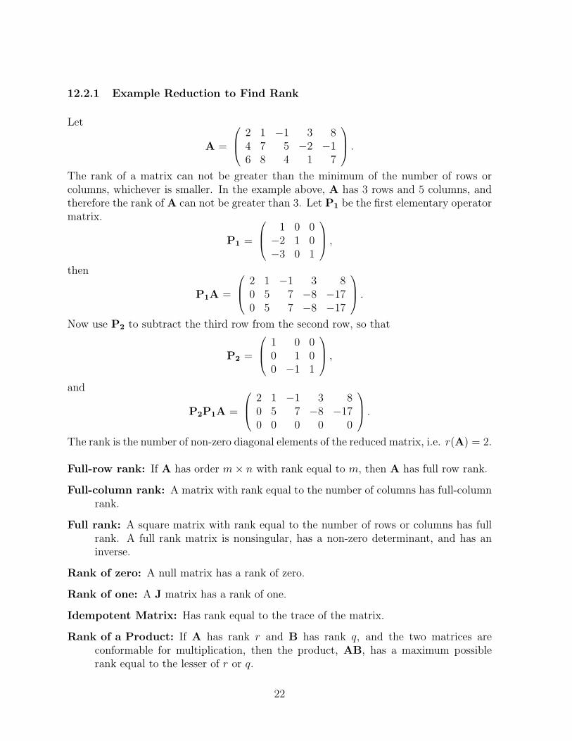
12.2.1 Example Reduction to Find Rank
Let
A =
2 1 −1 3 84 7 5 −2 −16 8 4 1 7
.The rank of a matrix can not be greater than the minimum of the number of rows orcolumns, whichever is smaller. In the example above, A has 3 rows and 5 columns, andtherefore the rank of A can not be greater than 3. Let P1 be the first elementary operatormatrix.
P1 =
1 0 0−2 1 0−3 0 1
,then
P1A =
2 1 −1 3 80 5 7 −8 −170 5 7 −8 −17
.Now use P2 to subtract the third row from the second row, so that
P2 =
1 0 00 1 00 −1 1
,and
P2P1A =
2 1 −1 3 80 5 7 −8 −170 0 0 0 0
.The rank is the number of non-zero diagonal elements of the reduced matrix, i.e. r(A) = 2.
Full-row rank: If A has order m× n with rank equal to m, then A has full row rank.
Full-column rank: A matrix with rank equal to the number of columns has full-columnrank.
Full rank: A square matrix with rank equal to the number of rows or columns has fullrank. A full rank matrix is nonsingular, has a non-zero determinant, and has aninverse.
Rank of zero: A null matrix has a rank of zero.
Rank of one: A J matrix has a rank of one.
Idempotent Matrix: Has rank equal to the trace of the matrix.
Rank of a Product: If A has rank r and B has rank q, and the two matrices areconformable for multiplication, then the product, AB, has a maximum possiblerank equal to the lesser of r or q.
22

12.3 Consequences of Linear Dependence
A matrix with rank less than the number of rows or columns in the matrix means thatthe matrix can be partitioned into a square matrix of order equal to the rank (with fullrank), and into other matrices of the remaining rows and columns. The other rows andcolumns are linearly dependent upon the rows and columns in that square matrix. Thatmeans that they can be formed from the rows and columns that are linearly independent.
Let A be a matrix of order p × q with rank r, and r is less than either p or q, thenthere are p− r rows of A and q− r columns which are not linearly independent. PartitionA as follows:
Ap×q =
(A11 A12
A21 A22
)such that A11 has order r × r and rank of r. Re-arrangement of rows and columns ofA may be needed to find an appropriate A11. A12 has order r × (q − r), A21 has order(p− r)× r, and A22 has order (p− r)× (q − r).
There exist matrices, K1 and K2 such that(A21 A22
)= K2
(A11 A12
),
and (A12
A22
)=
(A11
A21
)K1,
and
A =
(A11 A11K1
K2A11 K2A11K1
).
To illustrate, let
A =
3 −1 41 2 −1−5 4 −9
4 1 3
,and the rank of this matrix is 2. A 2 × 2 full rank submatrix within A is the upper left2× 2 matrix. Let
A11 =
(3 −11 2
),
then
A12 =
(4−1
)= A11K1,
where
K1 =
(1−1
),
23

A21 =
(−5 4
4 1
)= K2A11,
where
K2 =
(−2 1
1 1
),
andA22 = K2A11K1
=
(−2 1
1 1
)(3 −11 2
)(1−1
)=
(−9
3
).
This kind of partitioning of matrices with less than full rank is always possible. Inpractice, we need only know that this kind of partitioning is possible, but K1 and K2 donot need to be derived explicitly.
12.4 Calculation of a Generalized Inverse
For a matrix, A, of less than full rank, there is an infinite number of possible generalizedinverses, all of which would satisfy AA−A = A. However, only one generalized inverseneeds to be computed in practice. A method to derive one particular type of generalizedinverse has the following steps:
1. Determine the rank of A.
2. Obtain A11, a square, full rank submatrix of A with rank equal to the rank of A.
3. Partition A as
A =
(A11 A12
A21 A22
).
4. Compute the generalized inverse as
A− =
(A−1
11 00 0
).
If A has order p×q, then A− must have order q×p. To prove that A− is a generalizedinverse of A, then multiply out the expression
AA−A =
(A11 A12
A21 A22
)(A−1
11 00 0
)(A11 A12
A21 A22
)
=
(A11 A12
A21 A21A−111 A12
).
From the previous section, A21 = K2A11 so that
A21A−111 A12 = K2A11A
−111 A12 = K2A12 = A22.
24

12.5 Solutions to Equations Not of Full Rank
Because there are an infinite number of generalized inverses to a matrix that has lessthan full rank, then it logically follows that for a system of consistent equations, Ax = r,where the solutions are computed as x = A−r, then there would also be an infinite numberof solution vectors for x. Having computed only one generalized inverse, however, it ispossible to compute many different solution vectors. If A has q columns and if G is onegeneralized inverse of A, then the consistent equations Ax = r have solution
x = Gr + (GA− I)z,
where z is any arbitrary vector of length q. The number of linearly independent solutionvectors, however, is (q − r + 1).
Other generalized inverses of the same matrix can be produced from an existinggeneralized inverse. If G is a generalized inverse of A then so is
F = GAG + (I−GA)X + Y(I−AG)
for any X and Y. Pre- and post- multiplication of F by A shows that this is so.
12.6 Generalized Inverses of X′R−1X
The product X′R−1X occurs frequently where X is a matrix that usually has more rowsthan it has columns and has rank less than the number of columns, and R is a squarematrix that is usually diagonal. Generalized inverses of this product matrix have specialfeatures. Let X be a matrix of order N × p with rank r. The product, X′R−1X hasorder p× p and is symmetric with rank r. Let G represent any generalized inverse of theproduct matrix, then the following results are true.
1. G is not necessarily a symmetric matrix, in which case G′ is also a generalizedinverse of the product matrix.
2. X′R−1XGX′ = X′ or XGX′R−1X = X.
3. GX′R−1 is a generalized inverse of X.
4. XGX′ is always symmetric and unique for all generalized inverses of the productmatrix, X′R−1X.
5. If 1′ = k′X for some k′, then 1′R−1XGX′ = 1′.
25

13 Eigenvalues and Eigenvectors
There are a number of square, and sometimes symmetric, matrices involved in statisticalprocedures that must be positive definite. Suppose that Q is any square matrix then
• Q is positive definite if y′Qy is always greater than zero for all vectors, y.
• Q is positive semi-definite if y′Qy is greater than or equal to zero for all vectors y,and for at least one vector y, then y′Qy = 0.
• Q is non-negative definite if Q is either positive definite or positive semi-definite.
The eigenvalues (or latent roots or characteristic roots) of the matrix must be calcu-lated. The eigenvalues are useful in that
• The product of the eigenvalues equals the determinant of the matrix.
• The number of non-zero eigenvalues equals the rank of the matrix.
• If all the eigenvalues are greater than zero, then the matrix is positive definite.
• If all the eigenvalues are greater than or equal to zero and one or more are equal tozero, then the matrix is positive semi-definite.
If Q is a square, symmetric matrix, then it can be represented as
Q = UDU′
where D is a diagonal matrix, the canonical form of Q, containing the eigenvalues of Q,and U is an orthogonal matrix of the corresponding eigenvectors. Recall that for a matrixto be orthogonal then UU′ = I = U′U, and U−1 = U′.
The eigenvalues and eigenvectors are found by solving
| Q− dI | = 0,
andQu− du = 0,
where d is one of the eigenvalues of Q and u is the corresponding eigenvector. There arenumerous computer routines for calculating D and U.
In R, the eigen() function is used and both U and D are returned to the user.
26

14 Differentiation
The differentiation of mathematical expressions involving matrices follows similar rules asfor those involving scalars. Some of the basic results are shown below.
Letc = 3x1 + 5x2 + 9x3 = b′x
=(
3 5 9) x1
x2
x3
.With scalars, the derivatives are
∂c
∂x1
= 3
∂c
∂x2
= 5
∂c
∂x3
= 9,
but with vectors they are∂c
∂x= b.
The general rule is∂A′x
∂x= A.
Another function might be
c = 9x21 + 6x1x2 + 4x2
2
or
c =(x1 x2
)( 9 33 4
)(x1
x2
)= x′Ax.
With scalars the derivatives are
∂c
∂x1
= 2(9)x1 + 6x2
∂c
∂x2
= 6x1 + 2(4)x2,
and in matrix form they are,∂c
∂x= 2Ax.
If A was not a symmetric matrix, then
∂x′Ax
∂x= Ax + A′x.
27

15 Cholesky Decomposition
In simulation studies or applications of Gibb’s sampling there is frequently a need to factora symmetric positive definite matrix into the product of a matrix times its transpose. TheCholesky decomposition of a matrix, say V, is a lower triangular matrix such that
V = TT′,
and T is lower triangular. Suppose that
V =
9 3 −63 5 0−6 0 21
.The problem is to derive
T =
t11 0 0t21 t22 0t31 t32 t33
,such that
t211 = 9
t11t21 = 3
t11t31 = −6
t221 + t222 = 5
t21t31 + t22t32 = 0 and
t231 + t232 + t233 = 21
These equations give t11 = 3, then t21 = 3/t11 = 1, and t31 = −6/t11 = −2. From thefourth equation, t22 is the square root of (5− t221) or t22 = 2. The fifth equation says that(1)(−2) + (2)t32 = 0 or t32 = 1. The last equation says that t233 is 21− (−2)2 − (1)2 = 16.The end result is
T =
3 0 01 2 0−2 1 4
.The derivation of the Cholesky decomposition is easily programmed for a computer. Notethat in calculating the diagonals of T the square root of a number is needed, and con-sequently this number must always be positive. Hence, if the matrix is positive definite,then all necessary square roots will be of positive numbers. However, the opposite is nottrue. That is, if all of the square roots are of positive numbers, the matrix is not neces-sarily guaranteed to be positive definite. The only way to guarantee positive definitenessis to calculate the eigenvalues of a matrix and to see that they are all positive.
28

16 Inverse of a Lower Triangular Matrix
The inverse of a lower triangular matrix is also a lower triangular matrix, and can beeasily derived. The diagonals of the inverse are the inverse of the diagonals of the originalmatrix. Using the matrix T from the previous section, then
T−1 =
t11 0 0t21 t22 0t31 t32 t33
,where
tii = 1/tii
t21t11 + t22t
21 = 0
t31t11 + t32t
21 + t33t31 = 0
t32t22 + t33t
32 = 0.
These equations give
t11 =1
3
t21 = −1
6
t22 =1
2
t31 =5
24
t32 = −1
8and
t33 =1
4
Likewise the determinant of a triangular matrix is the product of all of the diagonalelements. Hence all diagonal elements need to be non-zero for the inverse to exist.
The natural logarithm of the determinant of a triangular matrix is the summationof the natural logarithms of the individual diagonal elements. This property is useful inderivative free restricted maximum likelihood.
29

17 EXERCISES
For each of the following exercises, first do the calculations by hand (or in your head).Then use R to obtain results, and check to make sure the results are identical.
1. Given matrices A and B, as follows.
A =
1 −1 0−2 3 −1−2 −2 4
, B =
6 −5 8−4 9 −3−5 −7 1
3 4 −5
.
If legal to do so, do the following calculations:
(a) A′.
(b) A + A′
(c) AA. Is A idempotent?
(d) AB.
(e) |A|.(f) B′A.
(g) Find the rank of B.
(h) A−1.
(i) B + B′.
(j) tr(BB′.
2. Given a new matrix, D.
D =
8 3 5 −1 74 1 2 −3 6−2 6 7 −5 2
1 −2 −4 0 31 6 14 −3 −4
Find the rank and a generalized inverse of D.
3. Find the determinant and an inverse of the following lower triangular matrix.
L =
10 0 0 0 0−2 20 0 0 0
1 −2 16 0 04 −1 −2 5 0−1 −6 3 1 4
30

4. If matrix R has N rows and columns with a rank of N − 2, and matrix W has Nrows and p columns for p < N with rank of p− 3, then what would be the rank ofW′R?
5. Create a square matrix of order 5 that has rank of 2, and show that the rank ofyour matrix is indeed 2.
6. Obtain a generalized inverse of matrix B in the first question, and show that itsatisfies the first Moore-Penrose condition.
31
Data Manipulations and R
18 Small Data Sets
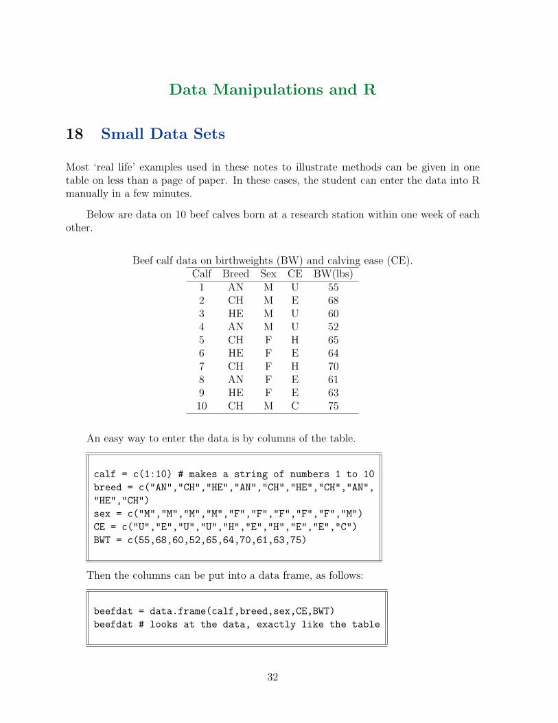
Most ‘real life’ examples used in these notes to illustrate methods can be given in onetable on less than a page of paper. In these cases, the student can enter the data into Rmanually in a few minutes.
Below are data on 10 beef calves born at a research station within one week of eachother.
Beef calf data on birthweights (BW) and calving ease (CE).Calf Breed Sex CE BW(lbs)
1 AN M U 552 CH M E 683 HE M U 604 AN M U 525 CH F H 656 HE F E 647 CH F H 708 AN F E 619 HE F E 6310 CH M C 75
An easy way to enter the data is by columns of the table.
calf = c(1:10) # makes a string of numbers 1 to 10
breed = c("AN","CH","HE","AN","CH","HE","CH","AN",
"HE","CH")
sex = c("M","M","M","M","F","F","F","F","F","M")
CE = c("U","E","U","U","H","E","H","E","E","C")
BWT = c(55,68,60,52,65,64,70,61,63,75)
Then the columns can be put into a data frame, as follows:
beefdat = data.frame(calf,breed,sex,CE,BWT)
beefdat # looks at the data, exactly like the table
32

The data frame can be saved and used at other times. The saved file can not beviewed because it is stored in binary format
setwd(choose.dir())
save(beefdat,file="beef.RData")
# and retrieved later as
load("beef.RData")
18.1 Creating Design Matrices
A desgin matrix is a matrix that relates levels of a factor to the observations. Theobservations, in this example, are the birthweights. The factors are breed, sex, and CE.The breed factor has 3 levels, namely AN, CH, and HE. The sex factor has 2 levels, Mand F, and the CE factors has 4 levels, U, E, H, and C.
A function to make a design matrix is as follows:
desgn <- function(v) {if(is.numeric(v)) { vn = v }else
{ vn = as.numeric(factor(v)) }
mrow = length(vn)
mcol = length(levels(vn))
X = matrix(data=c(0),nrow=mrow,ncol=mcol)
for(i in 1:mrow) {ic = vn[i]
X[i,ic] = 1 }return(X)
}
# To use, then
B = desgn(breed)
S = desgn(sex)
C = desgn(CE)
33

These matrices are
B =
1 0 00 1 00 0 11 0 00 1 00 0 10 1 01 0 00 0 10 1 0
, S =
1 01 01 01 00 10 10 10 10 11 0
, C =
1 0 0 00 1 0 01 0 0 01 0 0 00 0 1 00 1 0 00 0 1 00 1 0 00 1 0 00 0 0 1
.
Each row of a design matrix has one 1 and the remaining elements are zero. Thelocation of the 1 indicates the level of the factor corresponding to that observation. Ifyou summed together the elements of each row you will always get a vector of ones, or aJ matrix with just one column.
18.2 The summary Function
The data frame, beefdat, was created earlier. Now enter
summary(beefdat)
This gives information about each column of the data frame. If appropriate it givesthe minimum and maximum value, median, and mean of numeric columns. For non-numeric columns it gives the levels of that column and number of observations for each,or the total number of levels. This is useful to check if data have been entered correctlyor if there are codes in that data that were not expected.
The information may not be totally correct. For example, if missing birthweightswere entered as 0, then R does not know that 0 means missing and assumes that 0 wasa valid birthweight. The letters NA, signify a missing value, and these are skipped in thesummary function.
18.3 Means and Variances
The functions to calculate the means and variances are straightforward. Let y be a vectorof the observations on a trait of interest.
34

# The mean is
mean(y)
# The variance and standard deviation are
var(y)
sd(y)
18.4 Plotting
The plot function is handy for obtaining a visual appreciation of the data. There are alsothe hist(), boxplot(), and qqnorm() functions that plot information. Use the ?hist,for example, to find out more about a given function. This will usually show you all ofthe available options and examples of how the function is used. There are enough optionsand additional functions to make about any kind of graphical display that you like.
19 Large Data Sets
Large, in these notes, means a data set with more than 30 observations. This could bereal data that exists in a file on your computer. There are too many observations andvariables to enter it manually into R. The data set can be up to 100,000 records, but Ris not unlimited in space, and some functions may not be efficient with a large number ofrecords. If the data set is larger than 100,000 records, then other programming approacheslike FORTRAN or C++ should be considered, and computing should be on servers withmultiprocessors and gigabytes of memory.
For example, setting up a design matrix for a factor with a large data set may requiretoo much memory. Techniques that do not require an explicit representation of the designmatrix should be used. A chapter on analyses using this approach is given towards theend of the notes.
To read a file of trotting horse data, as an example, into R, use
zz = file.choose() # allows you to browse for file
# zz is the location or handle for the file
trot = read.table(file = zz, header=FALSE, col.names=
c("race","horse","year","month","track","dist","time"))
When a data frame is saved in R, it is written as a binary file, and the names of thecolumns form a header record in the file. Normally, data files do not have a header record,
35

thus, header=FALSE was indicated in the read.table() function, and the col.names hadto be provided, otherwise R provides its own generic header names like V1, V2, ....
19.1 Exploring the Data
summary(trot) # as before with the small data sets
dim(trot) # will indicate number of records and
# number of columns in trot data frame
horsef = length(factor(trot$horse)) # number of different horses
# in the data set
yearsf = length(factor(trot$year)) # number of different years
yearsf = factor(trot$year)
levels(yearsf) # list of years represented in data
tapply(trot$times,trot$track,mean) # mean racing times by
# track location
36

20 EXERCISES
1. Enter the data from the following table into a data frame.
Trotting horses racing times.Horse Sex Race Time(sec)
1 M 1 1352 S 1 1303 S 1 1334 M 1 1385 G 1 1322 S 2 1234 M 2 1315 G 2 1256 S 2 134
(a) Find the average time by race number and by sex of horse.
(b) Find the mean and variance of race times in the data.
(c) Create design matrices for horse, sex, and race.
(d) Do a histogram of race times.
(e) Save the data frame. Remove the data frame from your R-workspace usingrm(trot). Use ls() to determine that it is gone. Load the data frame backinto the R-workspace.
(f) Create a second data.frame by removing the ”sex” column from the first dataframe.
(g) Change the racing time of horse 6 in the second race to 136.
2. Read in any large data file, (provided by the instructor), and summarize the infor-mation as much as possible.
37

Writing a Linear Model
21 Parts of a Model
A linear model, in the traditional sense, is composed of three parts:
1. The equation.
2. Expectations and Variance-Covariance matrices of random variables.
3. Assumptions, restrictions, and limitations.
21.1 The Equation
The equation of the model contains the observation vector for the trait(s) of interest, thefactors that explain how the observations came to be, and a residual effect that includeseverything not explainable.
A matrix formulation of a general model equation is:
y = Xb + Zu + e
where
y is the vector of observed values of the trait,
b is a vector of factors, collectively known as fixed effects,
u is a vector of factors known as random effects,
e is a vector of residual terms, also random,
X,Z are known matrices, commonly known as design or indicator matrices, that relatethe elements of b and u to their corresponding element in y.
21.1.1 Observation Vector
The observation vector contains elements resulting from measurements, either subjectiveor objective, on the experimental units (usually animals) under study. The elements inthe observation vector are random variables that have a multivariate distribution, and ifthe form of the distribution is known, then advantage should be taken of that knowledge.
38

Usually y is assumed to have a multivariate normal distribution, but that is not alwaystrue.
The elements of y should represent random samples of observations from some definedpopulation. If the elements are not randomly sampled, then bias in the estimates of b andu can occur, which would lead to errors in ranking animals or conclusions to hypothesistests.
21.1.2 Factors
Discrete or Continuous A continuous factor is one that has an infinite-like range ofpossible values. For example, if the observation is the distance a rock can be thrown,then a continuous factor would be the weight of the rock. If the observation is therate of growth, then a continuous factor would be the amount of feed eaten.
Discrete factors usually have classes or levels such as age at calving might have fourlevels (e.g. 20 to 24 months, 25 to 28 months, 29 to 32 months, and 33 months orgreater). An analysis of milk yields of cows would depend on the age levels of thecows.
Fixed Factors In the traditional ”frequentist” approach, fixed and random factors needto be distinguished.
If the number of levels of a factor is small or limited to a fixed number, then thatfactor is usually fixed.
If inferences about a factor are going to be limited to that set of levels, and to noothers, then that factor is usually fixed.
If a new sample of observations were made (a new experiment), and the same levelsof a factor are in both samples, then the factor is usually fixed.
If the levels of a factor were determined as a result of selection among possibleavailable levels, then that factor should probably be a fixed factor.
Regressions of a continuous factor are usually a fixed factor (but not always).
Random Factors If the number of levels of a factor is large, then that factor can be arandom factor.
If the inferences about a factor are going to be made to an entire population ofconceptual levels, then that factor can be a random factor.
If the levels of a factor are a sample from an infinitely large population, then thatfactor is usually random.
If a new sample of observations were made (a new experiment), and the levels werecompletely different between the two samples, then the factors if usually random.
39

Examples of fixed and random factors.Fixed RandomDiets AnimalsBreeds Contemporary GroupsSex Herd-Year-SeasonsAge levels Permanent EnvironmentCages, Tanks Maternal EffectsSeasons Litters
21.2 Expectations and VCV Matrices
In general terms, the expectations are
E
yue
=
Xb00
,and the variance-covariance matrices are
V
(ue
)=
(G 00 R
),
where G and R are general square matrices assumed to be nonsingular and positivedefinite. Also,
V ar(y) = ZGZ′ + R = V.
21.3 Assumptions and Limitations
The third part of a model includes items that are not apparent in parts 1 and 2. Forexample, information about the manner in which data were sampled or collected. Werethe animals randomly selected or did they have to meet some minimum standards? Didthe data arise from many environments, at random, or were the environments speciallychosen? Examples will follow.
A linear model is not complete unless all three parts of the model are present. Sta-tistical procedures and strategies for data analysis are determined only after a completemodel is in place.
22 Example 1. Beef Calf Weights
Weights on beef calves taken at 200 days of age are shown in the table below.
40

Males Females198 187211 194220 202
185
22.1 Equation of the Model
yij = si + cj + eij,
where yij is one of the 200-day weights, si is an effect due to the sex of the calf (fixedfactor), cj is an effect of the calf (random factor), and eij is a residual effect or unexplainedvariation (random factor).
22.2 Expectations and Variances
E(cj) = 0
E(eij) = 0
V ar(cj) = σ2c
V ar(eij) = σ2ei
Additionally, Cov(cj, cj′) = 0, which says that all of the calves are independent of eachother, i.e. unrelated. Note that σ2
ei implies that the residual variance is different for eachsex of calf, because of the subscript i. Also, Cov(eij, eij′) = 0 and Cov(eij, ei′j′) = 0 saysthat all residual effects are independent of each other within and between sexes.
22.3 Assumptions and Limitations
1. All calves are assumed to be of the same breed.
2. All calves were reared in the same environment and time period.
3. All calves were from dams of the same age (e.g. 3 yr olds).
4. Maternal effects are ignored. Pedigree information is missing and maternal effectscan not be estimated.
5. Calf effects contain all genetic effects, direct and maternal.
6. All weights were accurately recorded (i.e. not guessed) at age 200 days.
41

22.4 Matrix Representation
Ordering the observations by males, then females, the matrix representation of the modelwould be
y =
198211220187194202185
, X =
1 01 01 00 10 10 10 1
,
and Z = I of order 7. Also,
G = Iσ2c = diag{σ2
c}R = diag{σ2
e1 σ2e1 σ
2e1 σ
2e2 σ
2e2 σ
2e2 σ
2e2}
23 Example 2. Temperament Scores of Dairy Cows
Below are progeny data of three sires on temperament scores (on a scale of 1(easy tohandle) to 40(very cantankerous)) taken at milking time.
CG Age Sire Score1 1 1 171 2 2 291 1 2 341 2 3 162 2 3 202 1 3 242 2 1 132 1 1 182 2 2 252 1 2 31
23.1 Equation of the Model
yijkl = ci + aj + sk + eijkl,
where yijkl is a temperament score, ci is a contemporary group effect (CG) which identifiesanimals that are typically reared and treated alike together; aj is an age group effect, in
42

this case just two age groups; sk is a sire effect; and eijkl is a residual effect. Contemporarygroups and age groups are often taken to be fixed factors, and sires are generally randomfactors. Age group 1 was for daughters between 18 and 24 mo of age, and age group 2was for daughters between 25 and 32 mo of age.
23.2 Expectations and Variances
E(yijkl) = ci + aj
E(sk) = 0
E(eijkl) = 0
V ar(sk) = σ2s
Cov(sk, sk′) = 0
V ar(eijkl) = σ2ei
Thus, the residual variance differs between contemporary groups. The sire variance rep-resents one quarter of the additive genetic variance because all progeny are assumed tobe half-sibs (i.e. from different dams). The sires are assumed to be unrelated.
23.3 Assumptions and Limitations
1. Daughters were approximately in the same stage of lactation when temperamentscores were taken.
2. The same person assigned temperament scores for all daughters.
3. The age groupings were appropriate.
4. Sires were unrelated to each other.
5. Sires were mated randomly to dams (with respect to milking temperament or anycorrelated traits).
6. Only one offspring per dam.
7. Only one score per daughter.
8. No preferential treatment towards particular daughters.
43

24 Example 3. Feed Intake in Pigs
24.1 Equation of the Model
yijkmn = (HYM)i + Sj + Lk + akm + pkm + eijkmn,
where yijkmn is a feed intake measurement at a specified moment in time, n, on the mth
pig from litter k, whose sow was in age group j, within the ith herd-year-month of birthsubclass; HYM is a herd-year-month of birth or contemporary group effect; Sj is an ageof sow effect identified by parity number of the sow; Lk is a litter effect which identifiesa group of pigs with the same genetic and environmental background; akm is an additivegenetic animal effect; pkm is an animal permanent environmental effect common to allmeasurements on an animal; and eijkmn is a residual effect specific to each measurement.
24.2 Expectations and Variances
E(Lk) = 0
V ar(Lk) = σ2L
E(akm) = 0
V ar(a) = Aσ2a
E(pkm) = 0
V ar(p) = Iσ2p
E(eijkmn) = 0
V ar(e) = R = Iσ2e
G =
Iσ2L 0 0
0 Aσ2a 0
0 0 Iσ2p
.All pigs were purebred Landrace. Two males and two females were taken randomly fromeach litter for feed intake measurements.
24.3 Assumptions and Limitations
1. There are no sex differences in feed intake.
2. There are no maternal effects on feed intake.
3. All measurements were taken at approximately the same age of the pigs.
44

4. All measurements were taken within a controlled environment at one location.
5. Feed and handling of pigs was uniform for all pigs within a herd-year-month subclass.
6. Litters were related through the use of boars from artificial insemination.
7. Feed intake was the average of 3 daily intakes during the week, and weekly averageswere available for 5 consecutive weeks.
8. Growth was assumed to be linear during the test period.
25 Comments on Models
1. Read the literature first to find out what should be in the model. Know what hasalready been researched.
2. Explain your model to other people in a workshop. Get ideas from other people.
3. Talk to industry people to know how data are collected.
4. Test your models. Do not be afraid to change the model as evidence accumulates.
5. Not everyone will agree to the same model.
6. Make sure you can justify all three parts.
7. Consider non linear or other types of models if appropriate.
26 EXERCISES
Write models for each of the following situations.
1. Dogs compete at tracking at several levels of skill. The lowest level is called a TD(Tracking Dog) trial. A track layer will set a track that is 600 to 800 meters inlength with at least two right angle turns in it and with two scent articles for thedog to indicate. The dog must pick up or lie down next to an article. The trackmust be at least one hour old before the dog runs it. The tracks are designed by ajudge based on the fields in which the tracks are set and weather conditions. Dogsof many breed compete. Someone decided to analyze data from two years of trialsin Canada. The results of 50 trialswere collected. Dogs either passed or failed thetest, so the observation is either 1 (if they pass) or 0 (if they fail). Write a modelto analyze these data.
45

2. Cows have been challenged with a foreign substance injected into their blood toinduce an immune response. Cows’ blood is sampled at 2 hr, 6 hr, 12 hr, 24 hr,and 48 hr. Levels of immune response are measured in each sample. Four differentlevels of the foreign substance have been used, and a fifth group of cows were givena placebo injection. Each group contained 3 cows. All cows were between 60 to 120days in milk.
3. Beef bulls undergo a 112 day growth test at stations located in 3 places in Ontario.The traits measured are the amount of growth on test and amount of feed eatenduring the test. Data are from several years, and bulls are known to be related toeach other across years. Several breeds and crossbreds are involved in the tests. Ageat start of the test is not the same for each bull, but between 150 to 250 days.
4. Weights of individually identified rainbow trout were collected over five years attwo years of age. Fish are reared in tanks in a research facility with the capabilityof controlling water temperature and hours of daylight. Tanks differ in size andnumber of fish. Pedigree information is available on all fish. Sex and maturity areknown. When a trout matures they stop growing.
5. Rabbit rearing for meat consumption is concerned with raising the most rabbits perlitter. Average litter size at birth may be 9, but the average number at weaning isonly 7. Litter size at weaning is the economically important trait measured on eachdoe.
6. Describe your own research project and write models for your data or experiment.
46

Estimation
27 Description of Problem
Below are data on gross margins (GM) of dairy cows. For each cow there are also observa-tions on protein yield, type score, non-return rate, milking speed, and somatic cell score.The problem is to regress the observed traits onto gross margins to derive a predictionequation. Given protein yield, type score, non-return rate, milking speed, and somaticcell score, predict the gross margins of the cow.
Gross Margins (GM) of dairy cows.Cow Prot Type Non-return Milking Somatic Gross
kg score rate speed Cell score Margins($)1 246 75 66 3 3.5 -2842 226 80 63 4 3.3 -4023 302 82 60 2 3.1 -2074 347 77 58 3 4.3 2675 267 71 66 5 3.7 -2016 315 86 71 4 3.5 2837 241 90 68 3 3.6 -458 290 83 70 2 3.9 2469 271 78 67 1 4.1 70
10 386 80 64 3 3.4 280
28 Theory Background
28.1 General Model
A general fixed effects model is
y = Xb + e
with E(y) = Xb, and V ar(y) = V = V (e). V is assumed to be positive definite, i.e. alleigenvalues are positive.
28.2 Function to be Estimated
Let a function of b be K′b, for some matrix K′.
47

28.3 Estimator
The estimator is a linear function of the observation vector, L′y, where L′ is to be deter-mined.
28.4 Error of Estimation
The error of estimation is given by L′y −K′b, and the variance-covariance matrix of theerror vector is
V ar(L′y −K′b) = V ar(L′y) = L′VL.
28.5 Properties of the Estimator
The following criteria are used to derive L′.
1. L′y should have the same expectation as K′b.
E(L′y) = L′E(y) = L′Xb,
and therefore, L′y is an unbiased estimator of K′b if L′X = K′.
2. The variance-covariance matrix of the error vector, L′VL, should have diagonalelements that are as small as possible. Minimization of the diagonal elements ofL′VL results in an estimator that is called best.
28.6 Function to be Minimized
F = L′VL + (L′X−K′)Φ
where Φ is a LaGrange Multiplier that imposes the restriction L′X = K′.
The function, F, is differentiated with respect to the unknowns, L and Φ, to give
∂F
∂L= 2VL + XΦ,
and∂F
∂Φ= X′L−K.
48

28.7 Solving for L′
The derivatives are equated to null matrices and rewritten as(V XX′ 0
)(Lθ
)=
(0K
)
where θ = .5Φ. Note that VL + Xθ = 0 from the first equation. Further,
L = −V−1Xθ
Substitution into the second row gives
X′L = −X′V−1Xθ = K,
so thatθ = − (X′V−1X)−K.
Putting θ into the equation for L, then
L = V−1X(X′V−1X)−K.
The estimator of K′b is then
L′y = K′(X′V−1X)−X′V−1y = K′b
whereb = (X′V−1X)−X′V−1y.
BLUE stands for Best Linear Unbiased Estimator. K′b is BLUE of K′b.
GLS stands for Generalized Least Squares, which are
(X′V−1X)b = X′V−1y
and b is the GLS solution.
Weighted LS is equivalent to GLS except that V is assumed to be a diagonal matrixwhose diagonal elements could be different from each other.
Ordinary LS is equivalent to GLS except that V is assumed to be an identity matrixtimes a scalar. That is, all of the diagonals of V are the same value.
49

29 BLUE for Example Data
The model isy = Xb + e,
withV ar(y) = V = Iσ2
e ,
X =
1 246 75 66 3 3.51 226 80 63 4 3.31 302 82 60 2 3.11 347 77 58 3 4.31 267 71 66 5 3.71 315 86 71 4 3.51 241 90 68 3 3.61 290 83 70 2 3.91 271 78 67 1 4.11 386 80 64 3 3.4
, y =
−284−402−207
267−201
283−4524670
280
.
Ordinary LS equations are sufficient for this problem.
X′X =
10 2891 802 653 30 36.402891 858337 231838 188256 8614 10547.60802 231838 64588 52444 2393 2915.00653 188256 52444 42795 1961 2377.1030 8614 2393 1961 102 108.20
36.4 10547.60 2915 2377.10 108.2 133.72
,
X′y =
79244244202593−679
469
,
y′y = 622, 729.
The solutions are given by
b = (X′X)−1 X′y,
50

b =
−4909.6115604.158675
14.33544120.8331251.493961
327.871209
.
If the solve() function in R is used, then the b above is obtained. If the solutionis obtained by taking the inverse of the coefficient matrix, X′X, then a different solutionvector is found. This solution vector is invalid due to rounding errors in the calculationof the inverse. To avoid rounding errors, subtract a number close to the mean of eachx−variable. For example, subtract 289 from all protein values, 80 from all type values,65 from NRR, 3 from milking speed values, and 3.6 from somatic cell scores. Then
X =
1 −43 −5 1 0 −0.11 −63 0 −2 1 −0.31 13 2 −5 −1 −0.51 58 −3 −7 0 0.71 −22 −9 1 2 0.11 26 6 6 1 −0.11 −48 10 3 0 0.01 1 3 5 −1 0.31 −18 −2 2 −2 0.51 97 0 −1 0 −0.2
,
and
X′X =
10 1 2 3 0 0.401 22549 −20 −526 −59 24.402 −20 268 74 −13 −4.203 −526 74 155 2 0.300 −59 −13 2 12 −1.00
0.4 24.40 −4.20 0.30 −1.00 1.24
,
X′y =
79041938602138−700
443
,
Notice that the elements in the coefficient matrix are much smaller, which leads toless rounding error. The solutions are the same except for the intercept, which is now−21.947742, which is related to the first solution in that
−4909.611560 = −21.947742− b1(289)− b2(80)− b3(65)− b4(3)− b5(3.6).
51

30 Analysis of Variance
30.1 Basic Table Format
All analysis of variance tables have a basic format.
Source Degrees of Sum of FormulaFreedom Squares
Total N SST y′V−1yMean 1 SSM y′V−11(1′V−11)−11′V−1y
Model r(X) SSR b′X′V−1y = y′V−1X(X′V−1X)−X′V−1yResidual N-r(X) SSE SST - SSR
For the example problem the table is as follows.
Analysis of Variance Table.Source df SSTotal 10 622,729.00Mean 1 4.90Model 6 620,209.10Residual 4 2519.90
Alternative tables can be found from different software packages. A common one isshown below, with corrections for the mean.
Alternative Analysis of Variance Table.Source df SSTotal-Mean 9 622,724.10Model-Mean 5 620,204.20Residual 4 2519.90
30.2 Requirements for Valid Tests of Hypothesis
The distribution of y should be multivariate normal. An F-statistic assumes that thenumerator sum of squares has a central Chi-square distribution, and the denominator sumof squares has a central Chi-square distribution, and the numerator and denominator areindependent.
A sum of squares, say y′Qy, has a Chi-square distribution if QV is idempotent.
52

30.2.1 Distribution of SSR
SSR = y′QRy
QR = V−1X(X′V−1X)−X′V−1.
SSR has a chi-square distribution if QRV is idempotent.
Proof:
QRVQRV = [V−1X(X′V−1X)−X′][V−1X(X′V−1X)−X′]
= [V−1X(X′V−1X)−][X′V−1X(X′V−1X)−X′]
= [V−1X(X′V−1X)−][X′]
= QRV.
30.2.2 Distribution of SSE
SSE = y′QEy,
QE = V−1 −QR.
SSE has a chi-square distribution if QEV is idempotent.
Proof:
QEVQEV = (V−1 −QR)V(V−1 −QR)V
= (I−QRV)(I−QRV)
= I−QRV −QRV + QRVQRV
= I− 2QRV + QRV
= I−QRV
= QEV
30.2.3 Independence of SSR and SSE
SSR and SSE are independent chi-square variables if QRVQE = 0.
53

Proof:
QRVQE = QRV(V−1 −QR)
= QR −QRVQR
= QR −QRVQRVV−1
= QR −QRVV−1
= QR −QR
= 0
30.2.4 Noncentrality parameters for SSR and SSE
The denominator of an F-statistic must be a central chi-square variable, while the numer-ator of the F-statistic will have a central chi-square distribution only if the null hypothesisis true. The noncentrality parameter of SSR, if the null hypothesis is false, is
λR = .5b′X′QRXb.
The noncentrality parameter of SSE is always zero.
Proof:
QEX = (V−1 −QR)X
= V−1X−V−1X(X′V−1X)−X′V−1X
= V−1X−V−1X
= 0
30.3 Testing the Model
To test the adequacy of the model,
FM =SSR/r(X)
SSE/(N − r(X)).
SSR could have a noncentral chi-square distribution. The noncentrality parameter isnon-null except when b = 0. If b = 0, then the model is non-significant.
A significant FM is one that differs from the table F-values, and indicates that b isnot a null vector and that the model does explain some of the major sources of variation.The model should usually be significant because b includes the mean of the observationswhich is usually different from zero.
54

The test of the model for the example data is
FM =620, 209.1/6
2519.9/4= 164.083,
which is highly significant.
30.4 R2 Values
The multiple correlation coefficient, R2, is another measure of the adequacy of a modelto fit the data.
R2 =SSR− SSMSST − SSM
.
The value goes from 0 to 1, and the higher the R2, the better is the fit of the modelto the data.
If the number of observations is small, then there is an adjustment for this situation.Let N be the number of observations and r be the number of regression coefficients(including intercept), then the adjusted R2 value is
R2∗ = 1− (N − 1)(1−R2)
(N − r).
For low R2, the adjusted value could be negative, which means it is actually 0, i.e. no fitat all.
31 General Linear Hypothesis Testing
The general linear hypothesis test partitions SSR into sub-hypotheses about functions ofb. An hypothesis test consists of
1. a null hypothesis,
2. an alternative hypothesis,
3. a test statistic, and
4. a probability level or rejection region.
55
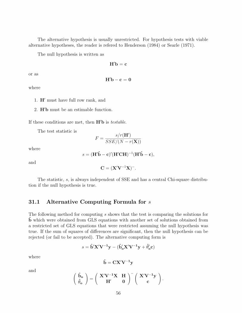
The alternative hypothesis is usually unrestricted. For hypothesis tests with viablealternative hypotheses, the reader is refered to Henderson (1984) or Searle (1971).
The null hypothesis is written as
H′b = c
or asH′b− c = 0
where
1. H′ must have full row rank, and
2. H′b must be an estimable function.
If these conditions are met, then H′b is testable.
The test statistic is
F =s/r(H′)
SSE/(N − r(X))
wheres = (H′b− c)′(H′CH)−1(H′b− c),
andC = (X′V−1X)−.
The statistic, s, is always independent of SSE and has a central Chi-square distribu-tion if the null hypothesis is true.
31.1 Alternative Computing Formula for s
The following method for computing s shows that the test is comparing the solutions forb which were obtained from GLS equations with another set of solutions obtained froma restricted set of GLS equations that were restricted assuming the null hypothesis wastrue. If the sum of squares of differences are significant, then the null hypothesis can berejected (or fail to be accepted). The alternative computing form is
s = b′X′V−1y − (b′oX′V−1y + θ′oc)
whereb = CX′V−1y
and (bo
θo
)=
(X′V−1X H
H′ 0
)− (X′V−1y
c
).
56

The equivalence of the alternative formula to that in the previous section is as follows.From the first row of the above equation,
X′V−1Xbo + H′θo = X′V−1y
which can be re-arranged and solved for bo as
bo = C(X′V−1y −Hθo)
= CX′V−1y −CHθo
= b−CHθo
and consequently from the second row of the restricted equations,
H′bo = c
= H′b−H′CHθo
Solving for θo givesθo = (H′CH)−1(H′b− c).
Now substitute this result into that for bo to obtain
bo = b−CH(H′CH)−1(H′b− c).
Taking the alternative form of s and putting in the new solutions for bo and θo the originallinear hypothesis formula is obtained, i.e.
s = SSR− (b′oX′V−1y + θ′oc)
= SSR− [b′ − (H′b− c)′(H′CH)−1H′C]X′V−1y
+(H′b− c)′(H′CH)−1c
= SSR− SSR + (H′b− c)′(H′CH)−1(H′b− c)
= (H′b− c)′(H′CH)−1(H′b− c)
31.2 Hypotheses having rank of X
Suppose there are two null hypotheses such that
H′1b = 0 with r(H′1) = r(X),
H′2b = 0 with r(H′2) = r(X),
butH′1 6= H′2,
then s1 is equal to s2 and both of these are equal to SSR. To simplify the proof, butnot necessary to the proof, let X have full column rank. Both null hypotheses represent
57

estimable functions and therefore, each H′i may be written as T′X for some T′, and T′Xhas order and rank equal to r(X). Consequently, T′X can be inverted. Then
si = b′Hi(H′iCHi)
−1H′ib
= b′X′T(T′XCX′T)−1T′Xb
= b′(X′T)[(X′T)−1C−(T′X)−1](T′X)b
= b′C−b
= y′V−1XC(C−)CX′V−1y
= y′V−1XCX′V−1y
= SSR
31.3 Orthogonal Hypotheses
Let H′b = 0 be a null hypothesis such that r(H′) = r(X) = r, and therefore,
s = (H′b)′(H′CH)−1H′b = SSR.
Now partition H′ into r rows as
H′ =
h′1h′2...
h′r
where each h′i has rank of one, then the rows of H′ are orthogonal if
h′iChj = 0 for all i 6= j.
If the rows are orthogonal to each other then
H′CH =
h′1Ch1 0 . . . 0
0 h′2Ch2 . . . 0...
.... . .
...0 0 . . . h′rChr
which means that
s = SSR =r∑i=1
(h′ib)2/(h′iChi).
When data are unbalanced, orthogonal contrasts are difficult to obtain and depend onthe number of observations in each subclass. Orthogonal contrasts are not essential forhypothesis testing. The subpartitions of SSR do not necessarily have to sum to SSR.
58
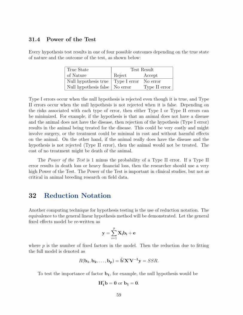
31.4 Power of the Test
Every hypothesis test results in one of four possible outcomes depending on the true stateof nature and the outcome of the test, as shown below:
True State Test Resultof Nature Reject AcceptNull hypothesis true Type I error No errorNull hypothesis false No error Type II error
Type I errors occur when the null hypothesis is rejected even though it is true, and TypeII errors occur when the null hypothesis is not rejected when it is false. Depending onthe risks associated with each type of error, then either Type I or Type II errors canbe minimized. For example, if the hypothesis is that an animal does not have a diseaseand the animal does not have the disease, then rejection of the hypothesis (Type I error)results in the animal being treated for the disease. This could be very costly and mightinvolve surgery, or the treatment could be minimal in cost and without harmful effectson the animal. On the other hand, if the animal really does have the disease and thehypothesis is not rejected (Type II error), then the animal would not be treated. Thecost of no treatment might be death of the animal.
The Power of the Test is 1 minus the probability of a Type II error. If a Type IIerror results in death loss or heavy financial loss, then the researcher should use a veryhigh Power of the Test. The Power of the Test is important in clinical studies, but not ascritical in animal breeding research on field data.
32 Reduction Notation
Another computing technique for hypothesis testing is the use of reduction notation. Theequivalence to the general linear hypothesis method will be demonstrated. Let the generalfixed effects model be re-written as
y =p∑i=1
Xibi + e
where p is the number of fixed factors in the model. Then the reduction due to fittingthe full model is denoted as
R(b1,b2, . . . ,bp) = b′X′V−1y = SSR.
To test the importance of factor b1, for example, the null hypothesis would be
H′1b = 0 or b1 = 0.
59

To obtain the appropriate reduction to test this hypothesis, construct a set of equationswith X1b1 omitted from the model. Let
W =(
X2 X3 . . . Xp
),
then the reduction due to fitting the submodel with factor 1 omitted is
R(b2,b3, . . .bp) = y′V−1W(W′V−1W)−W′V−1y
and the test statistic is computed as
s = R(b1,b2,b3, . . .bp)−R(b2,b3, . . .bp)
= R(b1 | b2,b3, . . .bp)
with r(X) − r(W) degrees of freedom. The above s is equivalent to the general linearhypothesis form because
R(b2,b3, . . .bp) = b′oX′V−1y
where bo is a solution to(X′V−1X H1
H′1 0
)(bo
θo
)=
(X′V−1y
0
).
The addition of H′1 as a LaGrange Multiplier to X′V−1X accomplishes the same pur-pose as omitting the first factor from the model and solving the reduced equationsW′V−1Wbs = W′V−1y, where bs is b excluding b1.
As long as the reductions due to fitting submodels are subtracted from SSR, the sames values will be calculated. The reduction notation method, however, assumes the nullhypothesis that H′b = 0 while the general linear hypothesis procedure allows the moregeneral null hypothesis, namely, H′b = c.
60

33 Example in R
# X is a matrix with N rows and r columns
# y is a vector of the N observations
# Ordinary LS equations are
XX = t(X) %*% X
Xy = t(X) %*% y
bhat = solve(XX,Xy)
# OR
C = ginv(XX)
bhat = C %*% Xy
# The two vectors should be identical.
# If they are not equal, then rounding errors are
# occurring
# AOV Table
SST = t(y) %*% y
SSR = t(bhat) %*% Xy
SSE = SST - SSR
SSM = sum(y)*mean(y)
sors = c("Total","Mean","Model","Residual")
df = c(N, 1, r, (N-r) )
SS = c(SST, SSM, SSR, SSE)
FF = c(0,0,((SSR/r)/(SSE/(N-r))) , 0)
AOV = cbind(sors,df,SS,FF)
AOV
# R-squared
R2 = (SSR - SSM)/(SST - SSM)
R2S = 1 - ( (N-1)*(1-R2)/(N-r) )
R2
R2S
61

# General Linear Hypothesis (assuming r=4, e.g.)
H0 = matrix(data=c(1, 0, 0, 0, 0, 1, 0, 0),byrow=TRUE,ncol=4)
c0 = matrix(data=c(250, 13),ncol=1)
w = (H0 %*% bhat) -c0
HCH = ginv(H0 %*% C %*% t(H0))
s = t(w) %*% HCH %*% w
df = 2 # two rows of H0
F = (s/df)/(SSE/(N-r)) # with df and (N-r) degrees of freedom
62
34 EXERCISES
1. Prove that s in the general linear hypothesis is Chi-square and is independent ofSSE. This is complicated and difficult.
2. Using the data from the example problem, test the hypothesis that
b1 = 5.
3. Using the data from the example problem, test the following hypothesis:
b2 = 0
b4 − b5 = 0
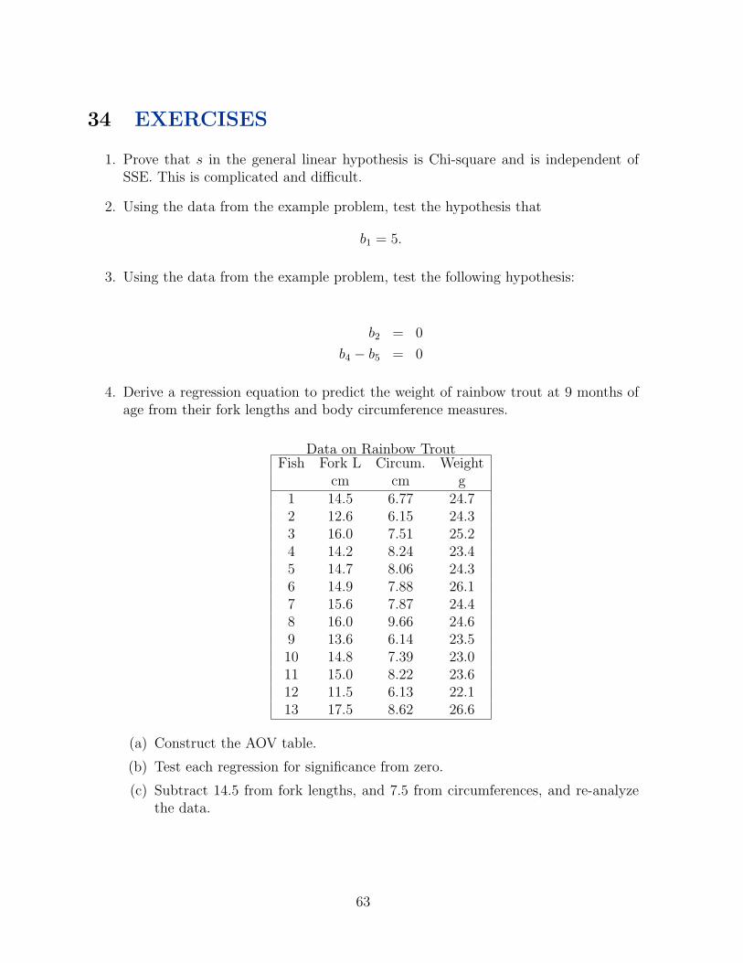
4. Derive a regression equation to predict the weight of rainbow trout at 9 months ofage from their fork lengths and body circumference measures.
Data on Rainbow TroutFish Fork L Circum. Weight
cm cm g1 14.5 6.77 24.72 12.6 6.15 24.33 16.0 7.51 25.24 14.2 8.24 23.45 14.7 8.06 24.36 14.9 7.88 26.17 15.6 7.87 24.48 16.0 9.66 24.69 13.6 6.14 23.510 14.8 7.39 23.011 15.0 8.22 23.612 11.5 6.13 22.113 17.5 8.62 26.6
(a) Construct the AOV table.
(b) Test each regression for significance from zero.
(c) Subtract 14.5 from fork lengths, and 7.5 from circumferences, and re-analyzethe data.
63

5. In a spline regression analysis inclusion of one of the x-variables depends on thevalue of another x-variable. In this problem, x2 is included only if x1 is greater than7, then x2 = X1 − 7, otherwise x2 = 0. The number 7 is called a knot, a point inthe curve where the shape changes direction. Below are the data and model.
Spline Regression Data.x1 x2
1 x2 x22 yi
8 64 1 1 1475 25 0 0 88
13 169 6 36 2026 36 0 0 1359 81 2 4 151
11 121 4 16 19818 324 11 121 9412 144 5 25 1737 49 0 0 1692 4 0 0 122
yi = a + b1x1 + b2x21 + b3x2 + b4x
22 + ei,
with V ar(y) = Iσ2e .
(a) Give the AOV table and R2 value.
(b) Test the hypothesis thata = 250.
(c) Test the hypothesis that
b1 = −5
b2 = 0
b2 − b4 = 3
64

6. Below are data on protein yields of a cow during the course of 365 days lactation.
Daily Protein Yields, kg for Agathe.Days in Milk(d) Yield(kg)
6 1.2014 1.2525 1.3238 1.4152 1.4973 1.35
117 1.13150 0.95179 0.88214 0.74246 0.65271 0.50305 0.40338 0.25360 0.20
yi = b0 + b1s + b2s2 + b3t + b4t
2 + ei,
and assume for simplicity that V ar(y) = Iσ2e . Also,
s = d/365
t = log(400/d)
(a) Analyze the data and give the AOV table.
(b) Estimate the protein on day 200 and the standard error of that estimate.
(c) Estimate the total protein yield from day 5 to day 305, and a standard errorof that estimate.
(d) Could this prediction equation be used on another cow? Could it be used ona clone of Agathe?
65

Estimability
35 Introduction
Consider models where the rank of X is less than the number of columns in X. Anexample is a two-way cross classified model without interaction where
yijk = µ+ Ai +Bj + eijk,
and
yijk is an observation on the postweaning gain (165 days) of male beef calves,
µ is an overall mean,
Ai is an effect due to the age of the dam of the calf,
Bj is an effect due to the breed of the calf, and
eijk is a residual effect specific to each observation.
There are four age of dam groups, namely 2-yr-olds, 3-yr-olds, 4-yr-olds, and 5-yr-oldsor greater, and three breeds, i.e. Angus(AN), Hereford(HE), and Simmental(SM). Thefollowing assumptions are made,
1. There are no breed by age of dam interactions.
2. Diet and management effects were the same for all calves.
3. All calves were raised in the same environment in the same months and year and atthe same age of development.
4. Calves resulted from random mating of sires to dams, and there is only one progenyper sire and per dam.
Also,
E(yijk) = µ+ Ai +Bj and
V ar(yijk) = σ2e ,
that is, the same residual variance was assumed for all calves regardless of breed groupor age of dam group. The data are given in the table below.
66

Growth Data on Beef CalvesCalf Age of Dam Breed of PWG
Tattoo (yr) calf (kg)16K 2 AN 34618K 3 AN 35522K 4 AN 363101L 5+ HE 388121L 5+ HE 38498L 2 HE 366115L 3 HE 371117L 3 HE 37552J 4 SM 41249J 5+ SM 42963J 2 SM 39670J 2 SM 404
Determine the effects of breed of calf and age of dam on postweaning gains of malecalves at a fixed age. The model in matrix notation is y = Xb + e, with
E(y) = Xb and V ar(y) = Iσ2e ,
where
Xb =
1 1 0 0 0 1 0 01 0 1 0 0 1 0 01 0 0 1 0 1 0 01 0 0 0 1 0 1 01 0 0 0 1 0 1 01 1 0 0 0 0 1 01 0 1 0 0 0 1 01 0 1 0 0 0 1 01 0 0 1 0 0 0 11 0 0 0 1 0 0 11 1 0 0 0 0 0 11 1 0 0 0 0 0 1
µA2
A3
A4
A5+
BAN
BHE
BSM
.
36 The Rank of X
Procedures for determining the rank of a matrix using elementary operators were given inprevious notes. In practice, the matrix X is too large to apply elementary operators. Also,in the use of classification models, X has mostly just zeros and ones in it. For one factorin a model, say diets, in a row of X there will be a single one, indicating the particulardiet, and the remaining elements in the row will be zero. If there were five diets, then
67

there would be five columns in X, and if those five columns were added together, theresult would be one column with all values equal to one.
If there were two factors, diets and breeds, in X, then the columns for the diet effectswould always sum to give one, and the columns for the breed effects would also sum togive one. Thus, there would be a dependency between diet effects and breed effects. Thedependencies need to be identified and removed. For example, if the column for diet 1 wasremoved from X, then there would not be a dependency between breed effects and dieteffects any longer. Any diet or any breed column could have been removed to eliminatethe dependency.
In the example problem of the previous section, the model equation is
yijk = µ+ Ai +Bj + eijk,
where age of dam has 4 levels, and breed of calf has 3 levels. The total number of columnsin X is 8. The columns of age of dam effects will have a dependency with the columns ofbreed of calf, and therefore, one of those columns has to be removed. Suppose the columnfor 2-yr-old age of dam is removed. The columns for breed of calf still sum to a column ofones, which is the same as the column for µ. Thus, another column (one of the breed ofcalf columns OR the µ column) needs to be removed. There are no further dependenciesafter removing the µ column. There were two restrictions imposed, so the rank of X istherefore, 6.
Given the model, and number of levels of each factor, it is possible to determine,before analyzing the data, the rank of X without using elementary operators. This takespractice, and problems are given in the Exercise section.
Another example is as follows. Let
yijk = µ+ Ai +Bij + eijk,
where factor A has 5 levels and factor B has 3 levels for every level of factor A. Thetotal number of columns in X is 1 + 5 + 5 ∗ (3) or 21. Factors A and B both have i as asubscript, and therefore, there is a dependency for every i, or 5 dependencies. All columnsfor factor A need to be removed. Also, summing all 15 columns of factor B gives a columnof ones, equivalent to the column for µ. Remove the column for µ and all dependenciesare removed. The rank of X is 15.
37 Estimable Functions
If the rank of X is less than the number of columns in X, then
• the inverse of X′X does not exist because its determinant is zero.
68

• a generalized inverse must be used, let
C = (X′X)−
such thatb = CX′y.
• there are an infinite number of generalized inverses of X′X, and therefore, an infinitenumber of possible solution vectors, b.
Recall that,
X′XCX′X = X′X
XCX′X = X
and XCX′ is invariant to C.
37.1 Solution vector
Ifb = CX′y,
thenE(b) = CX′Xb
is the first set of estimable functions.
37.2 Other Estimable Functions
Let K′b represent a set of functions of the elements of b, to determine if that function isestimable in terms of the working linear model, then show that
K′CX′X = K′.
If this equality does not hold, then the function K′b is not estimable.
Estimable functions are unique regardless of the solution vector or generalized inverseof X′X that is derived.
69

38 Generalized Least Squares Equations
38.1 Equations
Because V ar(y) = Iσ2e , the GLS equations reduce to ordinary LS equations, i.e. X′Xb =
X′y. For the example data,
X′X =
12 4 3 2 3 3 5 44 4 0 0 0 1 1 23 0 3 0 0 1 2 02 0 0 2 0 1 0 13 0 0 0 3 0 2 13 1 1 1 0 3 0 05 1 2 0 2 0 5 04 2 0 1 1 0 0 4
,X′y =
458915121101775
1201106418841641
,
and y′y = 1, 761, 549.
38.2 Generalized Inverse and Solution Vector
The rank of X in this example is 6. The dependencies are: columns 2, 3, 4, and 5 sumto give column 1 as do columns 6, 7, and 8. Two constraints on the solutions are needed.Let µ and A2 be set equal to zero, then a generalized inverse of (X′X) is C where C isequal to
0 0 0 0 0 0 0 00 0 0 0 0 0 0 00 0 .71366 .22467 .32159 −.31278 −.41410 −.136560 0 .22467 .79295 .19383 −.33921 −.16740 −.246700 0 .32159 .19383 .66960 −.17181 −.39648 −.215860 0 −.31278 −.33921 −.17181 .55066 .19383 .127750 0 −.41410 −.16740 −.39648 .19383 .52423 .140970 0 −.13656 −.24670 −.21586 .12775 .14097 .36564
.
The corresponding solution vector is b = CX′y, or
µ
A2
A3
A4
A5+
BAN
BHE
BSM
=
0.0.
9.026413.563924.4934
347.1366363.3921400.7357
.
70

38.3 Expectation of Solution Vector
The expectation of b isE(b) = E(CX′y) = CX′Xb.
For the example data, the expectations are
E
µ
A2
A3
A4
A5+
BAN
BHE
BSM
=
0 0 0 0 0 0 0 00 0 0 0 0 0 0 00 −1 1 0 0 0 0 00 −1 0 1 0 0 0 00 −1 0 0 1 0 0 01 1 0 0 0 1 0 01 1 0 0 0 0 1 01 1 0 0 0 0 0 1
µA2
A3
A4
A5+
BAN
BHE
BSM
=
00
A3 − A2
A4 − A2
A5+ − A2
µ+ A2 +BAN
µ+ A2 +BHE
µ+ A2 +BSM
.
Hence, A3 = 9.0264 is not an estimate of A3, but is rather an estimate of the differenceof A3 − A2. Also, BAN = 347.1366 is not an estimate of BAN , but of µ + A2 + BAN , anestimate of the mean of Angus calves from 2-yr-old dams.
By computing the expected value of the solution vector, the functions of the true pa-rameters that have been estimated by a particular generalized inverse can be determined.These functions are estimable because the solution vector is a linear function of y, whichis always estimable.
38.4 Other Solution Vectors
Other possible solution vectors are given by the formula,
bo = CX′y + (I−CX′X)z,
where z is any vector of arbitrary constants. For example, let
z′ =(
1 −2 6 0 1 −5 1 3),
71

then another solution vector is
bo = b +
1 0 0 0 0 0 0 00 1 0 0 0 0 0 00 1 0 0 0 0 0 00 1 0 0 0 0 0 00 1 0 0 0 0 0 0−1 −1 0 0 0 0 0 0−1 −1 0 0 0 0 0 0−1 −1 0 0 0 0 0 0
1−2
601−5
13
=
1−2
7.026411.563922.4934
348.1366364.3921401.7357
.
In order to check that bo is a valid solution vector, multiply bo by X′X which gives
X′Xbo = X′XCX′y + X′X(I−CX′X)z
= X′y + (X′X−X′XCX′X)z
= X′y
Hence, bo regenerates X′y and is therefore, a valid solution vector. Because z is anarbitrary vector, there are an infinite number of valid solution vectors to these equations.
38.5 Estimable Functions
The solution for A3 from b was 9.0264 which was an estimate of A3−A2. More generally,
k′b =(
0 −1 1 0 0 0 0 0)
b = A3 − A2.
The solution for A3 from bo was 7.0264, and the expectation is not known. However,
k′bo = Ao3 − Ao2 = 7.0264− (−2) = 9.0264,
and the expected value of k′bo is A3 − A2, the same as the expected value of k′b.
Suppose the following two functions are of interest.
k′1 =(
1 1 −1 0 0 1 0 0),
andk′2 =
(1 0 0 1 0 0 0 1
).
One way to quickly determine if these functions are not estimable is to multiply each ofthem times b and bo and if the results are different, then that function is not estimable.For the example data the results are
k′1b = 338.1102 and k′1bo = 340.1102,
andk′2b = 414.2996 and k′2b
o = 414.2996.
72

Thus, k′1b would definitely not be an estimable function because different results wereobtained with different solution vectors. The function, k′2b gave the same results for thesetwo solution vectors, and therefore might be an estimable function.
An exact method of determining estimability would be to check if
k′CX′X− k′ = 0 or k′CX′X = k′.
For the two functions in the previous paragraph,
k′1CX′X =(
1 2 −1 0 0 1 0 0)6= k′1,
andk′2CX′X = k′2.
Hence, k′2b is an estimable function.
38.6 Comments
Some basic results on estimability for classification models are
• µ is generally not estimable by itself.
• Differences among levels of main factors are estimable provided that factor has nointeractions with other factors.
• Only estimable functions have any meaning or value in an analysis.
• Only estimable functions can be tested.
39 Sum of Squares Due to Model
The infinite number of possible solution vectors to the GLS equations yield the same sumof squares due to the model. That is,
SSR = bo′X′y
= y′XCX′y + z′(I−X′XC)X′y
= y′XCX′y
because (I − X′XC)X′ = 0, and note that XCX′ = XC′X′ is unique for all possiblegeneralized inverses of X′X. For the example data,
SSR = b′X′y
= 1, 761, 457.9
= bo′X′y
73

This means that the test of the significance of the model is always unique, i.e. the testdoes not depend on the particular solution vector that has been calculated.
40 Least Squares Means
Least squares means are frequently reported in the scientific literature and are provided byseveral statistical packages. Least squares means are estimable functions and are thereforeunique. For the example data, the least squares means for age of dam effects would be
Least Squares MeansFor Age of Dam
Age of Dam Least Square Mean2 370.42153 379.44794 383.9854
5+ 394.9149
The functions that these numbers are estimating are not equal to µ+Ai because µ+Ai isnot an estimable function. Instead, these means are estimating µ+Ai + 1
3(BAN +BHE +
BSM).
Similarly, the least square means for the breed effects are estimating the function
µ+1
4(A2 + A3 + A4 + A5+) +Bj.
The values were 358.9075, 375.1630, and 412.5066 for AN, HE, and SM, respectively.
Least square means are not well understood by all researchers because estimabilityis not understood.
41 Variance of Estimable Functions
If k′b is an estimable function, then
k′CX′X = k′
or k′ = t′X witht′ = k′CX′.
74

Then
V ar(k′b) = k′V ar(b)k
= k′V ar(CX′y)k
= k′CX′V ar(y)XC′k
= k′CX′XC′kσ2e
= t′XC′kσ2e
= k′C′kσ2e
= k′Ckσ2e
If k′ =(
1 0 0 1 0 0 0 1)
and k′b = 425.2291, then
V ar(k′b) = (.79295 + .36564 + 2(−.24670))σ2e
= .66519σ2e .
Similarly, if
K′ =
(0 1 0 0 −1 0 0 00 0 0 0 0 0 −1 1
),
then
V ar(K′b) = K′CKσ2e
=
(.66960 −.18062−.18062 .60793
)σ2e
42 Analysis of Variance
AOV for Calf Postweaning Gain Data.Source Degrees of Sum of Squares Notation
FreedomTotal 12 1,761,549 SSTMean 1 1,754,910.08 SSMModel 6 1,761,457.9 SSRResidual 6 91.1 SSE
An estimate of σ2e is
σ2e =
SSE
(N − r(X))= 15.1833.
75

42.1 The Model
A test of the adequacy of the model is
FM =SSR/r(X)
SSE/(N − r(X))=
293, 576.32
15.1833= 19, 335.5.
Therefore, the model is highly significant. Another criterion would be the R2 where
R2 =SSR− SSMSST − SSM
= .9863.
Adjusting for the small sample size gives
R2∗ = .9748.
Thus, the model is very adequate at explaining variation in calf postweaning gains.
42.2 Partitioning SSR
Two tests of interest for the example data would be
1. Age of dam effects, and
2. Breed of calf effects.
42.2.1 Age of Dam Effects
The null hypothesis would be H′1b = 0 where
H′1 =
0 1 −1 0 0 0 0 00 1 0 −1 0 0 0 00 1 0 0 −1 0 0 0
,and
H′1b =
A2 − A3
A2 − A4
A2 − A5+
.H′1b is an estimable function, and therefore, the test is testable.
The sum of squares is
s1 = (H′1b)′(H′1GH1)−1H′1b
76

where
H′1b =
−9.0264−13.5639−24.4934
,
H′1GH1 =
.71366 .22467 .32159.22467 .79295 .19383.32159 .19383 .66960
,
(H′1GH1)−1 =
1.86667 −.33333 −.80000−.33333 1.41667 −.25000−.80000 −.25000 1.95000
,and s1 = 981.10653 with 3 degrees of freedom. The F -test is
F1 =s1/r(H
′1)
15.185022=
327.0355
15.185022= 21.5.
Age of dam effects, i.e. differences among age of dam groups, are significantly differentfrom zero.
Suppose the null hypothesis for age of dam effects had been written as H′2b = 0where
H′2 =
0 1 −1 0 0 0 0 00 0 1 −1 0 0 0 00 0 0 1 −1 0 0 0
,and
H′2b =
A2 − A3
A3 − A4
A4 − A5+
,then it can be shown that s2 = s1, and the same conclusions would be drawn with respectto the age of dam differences. To prove that s2 = s1, note that
H′2 = PH′1
where P is an elementary operator matrix,
P =
1 0 0−1 1 0
0 −1 1
,then
s2 = b′H1P′(PH′1CH1P
′)−1PH′1b
= b′H1P′P′−1(H′1CH1)−1P−1PH′1b
= b′H1(H′1CH1)−1H′1b
= s1.
Thus, the differences that are used in the null hypothesis only need to represent one setof linearly independent differences. All other differences can be generated by use of theappropriate elementary operator matrices.
77

42.2.2 Breed of Calf Effects
The hypothesis is
H′3 =
(0 0 0 0 0 1 −1 00 0 0 0 0 1 0 −1
),
H′3b =
(−16.2555−53.5991
),H′3CH3 =
(.68722 .37004.37004 .66079
),
and s3 = 4742.0565 with 2 degrees of freedom.
42.2.3 Summary
The tests are summarized in the table below.
Partitions of SSR for Calf PWG DataSource D.F. Sum of SquaresModel 6 1,761,457.9**Age of Dam 3 981.1065**Breed of Calf 2 4742.0565**
∗∗Significance at .05 level
43 Reduction Notation
Hypothesis testing may also be conducted using reduction notation as in the regressionmodels. For the example data, the model and submodels can be written as
Full Model y = µ1 + X1a + X2b + e where a refersto the vector of four age of dam effects, and brefers to the vector of three breed of calf effects.
Model 1 y = µ1 + X2b + e
Model 2 y = µ1 + X1a + e
Model 3 y = µ1 + e
The corresponding reductions for these models were obtained by constructing theordinary LS equations for each model, solving, and multiplying the solutions times theircorresponding right hand sides. The results gave
78

R(µ, a,b) = SSR = 1,761,457.9 6 dfR(µ,b) = 1,760,476.7935 3 dfR(µ, a) = 1,756,715.8435 4 dfR(µ) = SSM 1,754,910.08 1 df
To test the age of dam differences for significance from zero,
s1 = R(µ, a,b)−R(µ,b)
= R(a | µ,b)
= 981.1065
with 3 degrees of freedom (6-3).
For breed of calf differences,
s3 = R(µ, a,b)−R(µ, a)
= R(b | µ, a)
= 4742.0565
with 2 (6-4) degrees of freedom.
Lastly,
s = R(µ, a,b)−R(µ)
= R(a,b | µ)
= SSR− SSM= 6, 547.82
provides a test of the model excluding the mean with 5 (6-1) degrees of freedom.
All tests using reduction notation involve SSR in order to be equivalent to tests fromthe general linear hypothesis approach. All tests are for differences being not zero.
44 Connectedness
A procedure to determine connectedness was suggested by Weeks and Williams (1964).If all subclasses of the fixed effects are full, i.e. contain at least one observation, then thedata are completely connected and there are no problems of estimability.
When several subclasses are empty, i.e. do not contain any observations, then someestimable functions of b may no longer be estimable.
Following Weeks and Williams (1964): An N -tuple is a collection of numbers thatidentify a particular subclass. Suppose there are three fixed factors, then a general 3-tuple
79

that identifies a subclass is (i, j, k), where i indicates the level number of the first factor,j indicates the level number of the second factor, and k indicates the level number of thethird factor. Two N -tuples are said to be nearly identical if all of the level indicators arethe same except for one factor. The steps to determine connectedness are
1. Construct a table of all N -tuples that contain one or more observations.
2. Select any N -tuple from the table. The subclass with the largest number of obser-vations would be a logical choice.
3. Find all N -tuples in the table that are nearly identical to the selected N -tuple, thenany N -tuples that are nearly identical to these, and so on until no more nearlyidentical N -tuples can be found.
The resulting subset of N -tuples obtained in this manner form a connected set of sub-classes. If any other N=tuples remain in the table, then repeat the procedure on theremaining N -tuples, and continue until all N -tuples have been allocated to a connectedsubset.
The following list of 2-tuples is used to illustrate the procedure.
(1,1) (1,2) (1,5) (1,6)(2,2) (2,4) (2,6)
(3,3) (3,8)(4,1) (4,4) (4,5) (4,7)
(5,3) (5,8)
Pick one of the points from the table, say (1,1). The 2-tuples that are nearly identicalto (1,1) are
(1,2), (1,5), (1,6), and (4,1).
Now find the 2-tuples that are nearly identical to each of these four subclasses, andso on. The set of subclasses forms a connected subset consisting of
(1,1), (1,2), (1,5), (1,6), (4,1)(2,2), (4,5), (2,6), (4,4), (4,7)and (2,4).
The remaining points are (3,3), (3,8), (5,3), and (5,8) which form a second connectedsubset, but this subset is disconnected from the first.
There are a few options for handling disconnected subclasses.
80

1. Discard all of the small subsets and analyze only the largest group of connectedsubclasses.
2. Analyze each connected subset separately.
3. Collect more data for those subclasses that would improve connectedness betweenthe disconnected groups. In the previous example, the addition of observations tosubclasses (1,3), (2,3), (1,8), (2,8), and (3,5) would make all subclasses in the tableconnected.
The choice depends on the goals of the analysis and the costs of collecting more dataversus analyzing the available data.
The procedure of Weeks and Williams (1964) applies to a completely fixed effectsmodel without interactions or covariates. Connectedness may also be a problem in somemixed model situations and in the estimation of variance components. Computer pro-grams for checking connectedness are not trivial for large data sets. A simple, efficientprocedure for 2-tuples has been described by Fernando et al. (1983).
45 Classification Model with Interactions
Below are data on pheasants raised in two locations on three diets.
Example Data on PheasantsLocation Diet Males Females
1 1 3, 6, 4 2, 5, 12 1, 4, 5 1, 33 2, 4 1, 3, 2
2 1 5, 6, 4 2, 2, 42 2, 3, 6 33 4, 6, 5 2, 3, 3
Assume the model,
yijkm = µ+ Li +Dj + Sk + LDij + LSik +DSjk + LDSijk + eijkm
where
µ is the overall mean,
Li is a location effect,
81

Dj is a diet effect,
Sk is a sex effect, and
LDij, LSik, DSjk are the two-way interaction effects among the main factors, and
LDSijk is the three-way interaction of the main effects.
All factors are assumed to be fixed effects. The X matrix for this model is of order 32 by36 with a rank of 12, which is the number of three-way interaction subclasses.
An alternative (equivalent) form of the above model is
yijkm = µijk + eijkm
which has a corresponding X matrix of order 32 by 12 with a rank of 12. Assuming thatV ar(e) = Iσ2
e , then
X′X = diag(
3 3 3 2 2 3 3 3 3 1 3 3),
and(X′y)′ =
(13 8 10 4 6 6 15 8 11 3 15 8
),
where subclasses are ordered as in the table.
45.1 Solution Vector
The solutions to the LS equations are the subclass means in this case. For example, thesolution for location 1, diet 2, females was
µ122 = 4/2 = 2,
with expectation equal to
E(µ122) = µ+ L1 +D2 + S2 + LD12 + LS12 +DS22 + LDS122.
The expectation of all subclass means has a similar format to the above example. Noticethat all of the main effects and all of the interaction terms are involved. Consequently,there is no function of the µijk that can be formulated that would be totally free of theinteraction effects. For example,
E(µ211 − µ111) = µ+ L2 +D1 + S1 + LD21 + LS21 +DS11
+LDS211 − µ− L1 −D1 − S1 − LD11
−LS11 −DS11 − LDS111
= L2 − L1 + LD21 − LD11 + LS21 − LS11
+LDS211 − LDS111
82
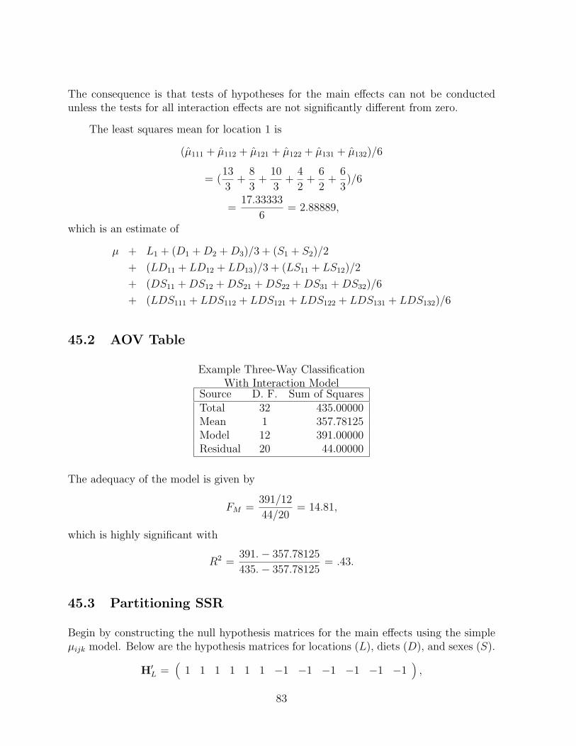
The consequence is that tests of hypotheses for the main effects can not be conductedunless the tests for all interaction effects are not significantly different from zero.
The least squares mean for location 1 is
(µ111 + µ112 + µ121 + µ122 + µ131 + µ132)/6
= (13
3+
8
3+
10
3+
4
2+
6
2+
6
3)/6
=17.33333
6= 2.88889,
which is an estimate of
µ + L1 + (D1 +D2 +D3)/3 + (S1 + S2)/2
+ (LD11 + LD12 + LD13)/3 + (LS11 + LS12)/2
+ (DS11 +DS12 +DS21 +DS22 +DS31 +DS32)/6
+ (LDS111 + LDS112 + LDS121 + LDS122 + LDS131 + LDS132)/6
45.2 AOV Table
Example Three-Way ClassificationWith Interaction Model
Source D. F. Sum of SquaresTotal 32 435.00000Mean 1 357.78125Model 12 391.00000Residual 20 44.00000
The adequacy of the model is given by
FM =391/12
44/20= 14.81,
which is highly significant with
R2 =391.− 357.78125
435.− 357.78125= .43.
45.3 Partitioning SSR
Begin by constructing the null hypothesis matrices for the main effects using the simpleµijk model. Below are the hypothesis matrices for locations (L), diets (D), and sexes (S).
H′L =(
1 1 1 1 1 1 −1 −1 −1 −1 −1 −1),
83

H′D =
(1 1 −1 −1 0 0 1 1 −1 −1 0 01 1 0 0 −1 −1 1 1 0 0 −1 −1
),
andH′S =
(1 −1 1 −1 1 −1 1 −1 1 −1 1 −1
).
The matrices for testing the interaction effects are obtained from the matrices for themain effects by computing the product of each row of one matrix times each row of thesecond matrix, element by element. The matrix for testing location by diet interactionwould be formed by the product of rows of H′L times H′D. Because the matrix for locationshas one row and that for diets has two rows, the resulting matrix will have 2(= 1 × 2)rows, as follows:
H′LD =
(1 1 −1 −1 0 0 −1 −1 1 1 0 01 1 0 0 −1 −1 −1 −1 0 0 1 1
).
Similarly, for location by sex and diet by sex interactions,
H′LS =(
1 −1 1 −1 1 −1 −1 1 −1 1 −1 1),
and
H′DS =
(1 −1 −1 1 0 0 1 −1 −1 1 0 01 −1 0 0 −1 1 1 −1 0 0 −1 1
).
The matrix for testing the three-way interaction can be formed in a number of ways,one of which is to multiply H′LD times H′S giving
H′LDS =
(1 −1 −1 1 0 0 −1 1 1 −1 0 01 −1 0 0 −1 1 −1 1 0 0 −1 1
).
Partitions of SSRThree-way model with interaction example.
Source D.F. Sum of Squares F-valuesL,locations 1 4.3556 1.98D,diets 2 2.4482 0.56S,sexes 1 17.4222 7.92*LD 2 1.4380 0.33LS 1 0.3556 0.16DS 2 1.1468 0.26LDS 2 1.1013 0.25
None of the interaction effects were significantly different from zero. Tests of themain effects may be interpretted ignoring the interactions.
If the three-way interaction was significant, then all of the other tests would notbe needed because they could not be interpretted without reference to the three-wayinteractions.
84

45.4 Missing Subclasses
If one or more subclasses had been empty, i.e. no observations present, then the for-mulation of the hypothesis test matrices and the interpretation of results becomes morecomplicated, and in some cases tests may not be possible at all.
As the number of missing subclasses increases, one must ”customize” the contraststo be those of the most interest. Another possibility is to remove data until all remainingsubclasses are full. This could have the effect of eliminating one or more levels of severalfactors which may not be desirable. If too many subclasses are missing, then a model thatignores interactions could be analyzed. Interpretation of results would need to considerthe possibility that interactions might exist.
46 Classification Model with Covariates
Consider a nutrition trial of dairy heifers designed to study growth and development ofthe mammary gland relative to the plane of nutrition. The amount of adipose tissue inthe mammary gland is one of the traits of interest which is dependent upon the amountof growth hormone in the blood as well as the diet. A model might be as follows:
yij = µ+ Ti + b(Xij) + eij
where
yij is the amount of adipose tissue,
µ is the overall mean,
Ti is the effect of diet, i = 1, 2, 3,
b is the regression coefficient of yij on Xij, and
eij is a residual effect.
Assume that V ar(eij) = σ2e , and that all residual effects are uncorrelated. The levels of
growth hormone in the blood are assumed to be unaffected by the diets in the study.If there were an effect, then the inclusion of growth hormone levels as a covariate couldreduce the effects of diets in the analysis. A way to counteract this problem would be toestimate a separate regression coefficient for each diet.
85

Example data on dairy heifers.Heifer Diet Adipose Growth
Number Tissue Hormone1 1 147 552 1 150 473 1 145 564 1 166 50
5 2 114 536 2 140 487 2 105 498 2 130 549 2 133 58
10 3 101 4211 3 97 4512 3 112 5113 3 90 57
46.1 Equations and Solution Vector
13 4 5 4 6654 4 0 0 2085 0 5 0 2624 0 0 4 195
665 208 262 195 34303
µ
T1
T2
T3
b
=
1, 630
608622400
83, 645
with solutions
µ
T1
T2
T3
b
=
0.0000
165.1677137.6690112.3447−.2532
.
The expectation of this particular solution vector is E(b) = (X′X)−X′Xb or
E
µ
T1
T2
T3
b
=
0 0 0 0 01 1 0 0 01 0 1 0 01 0 0 1 00 0 0 0 1
µT1
T2
T3
b
.
86
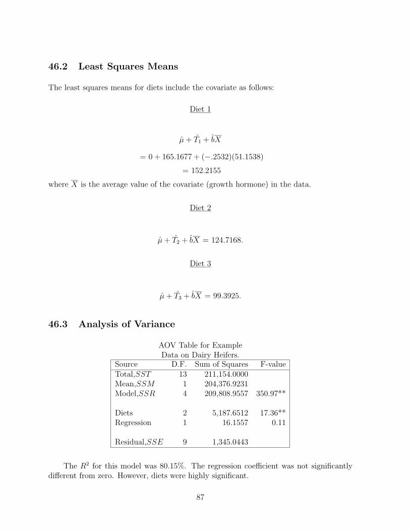
46.2 Least Squares Means
The least squares means for diets include the covariate as follows:
Diet 1
µ+ T1 + bX
= 0 + 165.1677 + (−.2532)(51.1538)
= 152.2155
where X is the average value of the covariate (growth hormone) in the data.
Diet 2
µ+ T2 + bX = 124.7168.
Diet 3
µ+ T3 + bX = 99.3925.
46.3 Analysis of Variance
AOV Table for ExampleData on Dairy Heifers.
Source D.F. Sum of Squares F-valueTotal,SST 13 211,154.0000Mean,SSM 1 204,376.9231Model,SSR 4 209,808.9557 350.97**
Diets 2 5,187.6512 17.36**Regression 1 16.1557 0.11
Residual,SSE 9 1,345.0443
The R2 for this model was 80.15%. The regression coefficient was not significantlydifferent from zero. However, diets were highly significant.
87

47 EXERCISES
1. Rank of the Model
Determine the number of columns in X and the rank of X for the following modelequations where all factors are fixed factors:
(a) yijkl = µ+ Ai +Bj + Ck + eijkl where i = 1, 5, j = 1, 4, k = 1, 8.
(b) yijkl = µ+ Ai +Bj + Ck + (AC)ik + eijkl where i = 1, 5, j = 1, 3, k = 1, 6.
(c) yijklm = µ+(AB)ij+(CD)kl+(BC)jk+eijklm where i = 1, 3, j = 1, 4, k = 1, 6,l = 1, 5.
(d) yijklm = Ai + Bij + Cijk + Dl + eijklm where i = 1, 2, j = 1, 3, k = 1, 4, andl = 1, 9.
(e) yijkl = µ+Ai +BC(jk) + b1x1ijkl + b2x2ijkl + eijkl where i = 1, 6, j = 1, 2, andk = 1, 4.
(f) yijkl = µ +Ti +Hj +HYjk + eijkl where i = 1, 10, j = 1, 20, and k = 1, 15.
2. Disconnectedness
Determine the connected groups within each of the following sets of filled subclassnumbers
(a)
(1,1,1) (2,2,2) (3,3,4) (4,3,1)(1,3,2) (2,1,4) (3,1,1) (4,4,1)(1,3,1) (2,1,1) (3,2,4) (4,2,3)(1,1,4) (2,4,1) (3,3,3) (4,4,4)(1,2,3) (2,3,1) (3,1,4) (4,3,2)(1,4,1) (2,2,3) (3,3,1) (4,4,3)(1,2,1) (2,3,2) (3,4,2) (4,1,1)
(b)
(A,1,6) (A,2,5) (B,3,4) (B,1,5) (C,2,6)(C,3,4) (D,2,1) (D,1,6) (A,3,3) (B,2,6)(C,1,5) (D,3,1) (A,2,4) (B,1,6) (C,1,4)(D,1,1) (A,3,1) (B,4,4) (C,3,3) (D,4,2)
88

(c)
(1,1,1,1) (1,2,1,2) (2,1,3,1) (2,3,3,1) (3,2,2,1)(1,3,3,3) (1,2,1,3) (3,2,1,2) (1,3,3,1) (2,3,1,1)(2,2,3,1) (2,2,2,2) (1,2,3,1) (2,1,2,2) (2,2,3,1)(3,2,3,1) (2,3,1,3) (1,3,2,1) (3,3,3,2) (1,1,1,2)
3. Classification Model
(a) Guinea pigs were given different types of water, and small amounts of one ofthree varieties of nuts (as a snack). They were housed in separate cages withinone of four rooms that were kept at different temperatures. Below are recordson the amount of regular feed eaten per day. The factors in the model areRoom (R), Water Type (W)(either tap water or Perrier), and Nut Variety (V)(either almonds, walnuts, or cashews). Nuts and water are offered through theday - equal amounts to each guinea pig.
The objective is to estimate and test differences in regular feed intake (g) dueto room, water type, and nut variety.
Guinea Pig Data on Daily Feed IntakeRoom Water Nuts Obs. Room Water Nuts Obs.
1 1 1 117 2 2 2 1781 2 2 110 2 2 3 821 1 3 71 2 1 2 411 2 2 170 2 1 3 911 1 3 150 2 1 1 1161 2 3 130 2 2 1 611 1 3 64 2 2 2 1151 2 2 89 2 1 2 871 1 1 1413 2 2 48 4 2 3 593 2 1 75 4 1 1 903 1 3 139 4 2 2 1383 1 3 55 4 2 3 773 2 2 53 4 1 1 1293 2 2 84 4 2 1 823 1 3 62 4 2 3 453 1 1 125 4 1 1 673 2 1 103 4 2 3 180
4 2 2 123
Let the model equation be:
yijkl = Ri + Wj + Vk + eijkl
Assume the residual variance is constant for all subclasses (i.e. Iσ2e).
89

i. Construct the OLS equations and obtain a solution.
ii. Test for differences among rooms.
iii. Test for differences among water types.
iv. Test for difference among nut varieties.
v. Write a complete AOV table, and compute the multiple R2 coefficient.
vi. Write a “Conclusions” paragraph about this analysis.
(b) Below are scores of warmblood mares from Inspection Tests given in threelocations, (Lj). Age of the horse at test, (Ai), is another important variable.
Mare Age Location Score1 2 Alberta 712 3 Alberta 833 4 Alberta 924 2 Alberta 745 3 Sask. 686 4 Sask. 787 2 Sask. 808 3 Sask. 949 4 Man. 8910 2 Man. 7711 3 Man. 8512 4 Man. 86
Let the model equation be
yijk = µ + Ai + Lj + eijk.
The total sum of squares is 80,285.
i. Set up X′X and X′y.
ii. Assume that the solution vector was as follows:
µ
A1
A2
A3
LALLSKLMB
=
0.00.05.49.3
71.372.475.5
,
Construct the basic AOV table.
iii. Calculate R2.
iv. Write the null hypothesis, (H′0), for testing the effect of location.
90

v. Calculate the Least Squares Mean for LAL.
(c) Every time that I go to the cottage I have to clear the cottage of mice. Everymouse that is killed, I measure its tail length and record its sex. Below is atable of my findings over the last four years. Numbers in parentheses are thenumber of mice, and the first number is the sum of the tail lengths of thosemice.
Sex 2004 2005 2006 2007 Row TotalsFemales 54(12) 42(9) 51(10) 47(9) 194(40)Males 34(8) 50(11) 46(10) 41(11) 171(40)ColumnTotals 88(20) 92(20) 97(20) 88(20) 365(80)
Construct Ordinary Least Squares equations from the numbers in the table fora model with sex and year fixed effects.
(d) Below are quantities calculated for an analysis of data on squirrels. Use thesequantities to complete the Analysis of Variance Table below.
y′y = 54, 079
N = 22
b′X′y = 43, 266.84
r(X) = 8
y′11′y/N = 32, 417.26
Analysis of Variance TableSource degrees of Sum of Squares Mean Squares F-value
freedomTotal
Model
Residual
What is the R2 value for this analysis?
(e) We know thatE(b) = CX′Xb,
91

for C = (X′X)−, and for a given analysis it was found that
CX′X =
0 0 0 0 0 0 0 00 1 −1 0 0 0 0 00 0 0 0 0 0 0 00 0 0 0 0 0 0 00 0 0 −1 1 0 0 00 0 0 −1 0 1 0 01 0 1 1 0 0 1 01 0 1 1 0 0 0 1
.
Determine if K′b is estimable if
K′ =
(0 1 −1 −2 1 1 0 02 0 2 0 1 1 1 1
).
(f) Please use the data in Table AA. The first number is the number of observa-tions, and the second number in parentheses is the SUM of the observations inthat subclass.
92

Table AAFarm Breeds Totals
1 2 31 5(105) 5(155) 30(780) 40(1040)2 5( 45) 15(285) 10(140) 30(470)Totals 10(150) 20(440) 40(920) 70(1510)
i. Construct the OLS equations (order 6) for the model
yijk = (BF )ij + eijk,
where both factors are fixed.
ii. Assume the total sum of squares is 37842, and a solution vector is equalto the subclass means (and µ = 0), and its expectation are
b =
219
31192614
=
BF11
BF12
BF21
BF22
BF31
BF32
.
Construct the basic ANOVA table from this information.
iii. Construct the null hypothesis matrices for the two main effects (breed andfarm), and the one for the interaction between breed and farm.
iv. What are the R2 and estimate of residual variance for this analysis?
93
Prediction Theory
48 Introduction
Best Linear Unbiased Prediction (BLUP) was developed for animal breeding by Dr.Charles Roy Henderson around 1949. The methods were first applied to genetic eval-uation of dairy sires in the northeastern United States in 1970. BLUP is used in nearlyall countries and all livestock species for genetic evaluation of individual animals.
DEFINITION: Prediction is the estimation of the realized value of a randomvariable (from data) that has been sampled from a population with a known variance-covariance structure.
49 General Linear Mixed Model
49.1 Equation of the Model
y = Xb + Zu + e
where
y is an N × 1 vector of observations,
b is a p× 1 vector of unknown constants,
u is a q × 1 vector of unknown effects of random variables,
e is an N × 1 vector of unknown residual effects,
X,Z are known matrices of order N × p and N × q respectively, that relate elements ofb and u to elements of y.
The elements of b are considered to be fixed effects while the elements of u arethe random effects from populations of random effects with known variance-covariancestructures. Both b and u may be partitioned into one or more factors depending on thesituation.
94

49.2 Expectations and Covariance Structure
The expectations of the random variables are
E(u) = 0
E(e) = 0
E(y) = E(Xb + Zu + e)
= E(Xb) + E(Zu) + E(e)
= XE(b) + ZE(u) + E(e)
= Xb + Z0 + 0
= Xb
and the variance-covariance structure is typically represented as
V
(ue
)=
(G 00 R
),
where G and R are known, positive definite matrices. Consequently,
V ar(y) = V ar(Xb + Zu + e)
= V ar(Zu + e)
= ZV ar(u)Z′ + V ar(e) + ZCov(u, e) + Cov(e,u)Z′
= ZGZ′ + R, and
Cov(y,u) = ZG
Cov(y, e) = R
If u is partitioned into s factors as
u′ =(
u′1 u′2 · · · u′s),
then
V ar(u) = V ar
u1
u2...
us
=
G11 G12 · · · G1s
G′12 G22 · · · G2s...
.... . .
...G′1s G′2s · · · Gss
.Each Gij is assumed to be known.
50 Predictors
The problem is to predict the function
K′b + M′u,
provided that K′b is an estimable function.
95

50.1 Best Predictor
The best predictor, for any type of model, requires knowledge of the distribution of therandom variables as well as the moments of that distribution. Then, the best predictoris the conditional mean of the predictor given the data vector, i.e.
E(K′b + M′u|y)
which is unbiased and has the smallest mean squared error of all predictors (Cochran1951). The computational form of the predictor depends on the distribution of y. Thecomputational form could be linear or nonlinear. The word best means that the predictorhas the smallest mean squared error of all predictors of K′b + M′u.
50.2 Best Linear Predictor
The best predictor may be linear OR nonlinear. Nonlinear predictors are often difficult tomanipulate or to derive a feasible solution. The predictor could be restricted to class oflinear functions of y. Then, the distributional form of y does not need to be known, andonly the first (means) and second (variances) moments of y must be known. If the firstmoment is Xb and the second moment is V ar(y) = V, then the best linear predictoris
E(K′b + M′u) = K′b + C′V−1(y −Xb)
whereC′ = Cov(K′b + M′u,y).
When y has a multivariate normal distribution, then the best linear predictor (BLP) isthe same as the best predictor (BP). The BLP has the smallest mean squared error of alllinear predictors of K′b + M′u.
50.3 Best Linear Unbiased Predictor
In general, the first moment of y, namely Xb, is not known, but V, the second moment,is commonly assumed to be known. Then predictors can be restricted further to thosethat are linear and also unbiased. The best linear unbiased predictor is
K′b + C′V−1(y −Xb)
whereb = (X′V−1X)−X′V−1y,
and C and V are as before.
96

This predictor is the same as the BLP except that b has replaced b in the formula.Note that b is the GLS estimate of b. Of all linear, unbiased predictors, BLUP has thesmallest mean squared error. However, if y is not normally distributed, then nonlinearpredictors of K′b + M′u could potentially exist that have smaller mean squared errorthan BLUP.
51 Derivation of BLUP
51.1 Predictand and Predictor
DEFINITION: The predictand is the function to be predicted, in this case
K′b + M′u.
DEFINITION: The predictor is the function to predict the predictand, a linear functionof y, i.e. L′y, for some L.
51.2 Requiring Unbiasedness
Equate the expectations of the predictor and the predictand to determine what needs tobe true in order for unbiasedness to hold. That is,
E(L′y) = L′Xb
E(K′b + M′u) = K′b
then to be unbiased for all possible vectors b,
L′X = K′
orL′X−K′ = 0.
51.3 Variance of Prediction Error
The prediction error is the difference between the predictor and the predictand. Thecovariance matrix of the prediction errors is
V ar(K′b + M′u− L′y) = V ar(M′u− L′y)
= M′V ar(u)M + L′V ar(y)L
−M′Cov(u,y)L− L′Cov(y,u)M
= M′GM + L′VL−M′GZ′L− L′ZGM
= V ar(PE)
97

51.4 Function to be Minimized
Because the predictor is required to be unbiased, then the mean squared error is equivalentto the variance of prediction error. Combine the variance of prediction error with aLaGrange Multiplier to force unbiasedness to obtain the matrix F, where
F = V ar(PE) + (L′X−K′)Φ.
Minimization of the diagonals of F is achieved by differentiating F with respect tothe unknowns, L and Φ, and equating the partial derivatives to null matrices.
∂F
∂L= 2VL− 2ZGM + XΦ = 0
∂F
∂Φ= X′L−K = 0
Let θ = .5Φ, then the first derivative can be written as
VL = ZGM−Xθ
then solve for L as
V−1VL = L
= V−1ZGM−V−1Xθ.
Substituting the above for L into the second derivative, then we can solve for θ as
X′L−K = 0
X′(V−1ZGM−V−1Xθ)−K = 0
X′V−1Xθ = X′V−1ZGM−K
θ = (X′V−1X)−(X′V−1ZGM−K)
Substituting this solution for θ into the equation for L gives
L′ = M′GZ′V−1 + K′(X′V−1X)−X′V−1
−M′GZ′V−1X(X′V−1X)−X′V−1.
Letb = (X′V−1X)−X′V−1y,
then the predictor becomes
L′y = K′b + M′GZ′V−1(y −Xb)
which is the BLUP of K′b + M′u, and b is a GLS solution for b. A special case for thispredictor would be to let K′ = 0 and M′ = I, then the predictand is K′b + M′u = u,and
L′y = u = GZ′V−1(y −Xb).
Hence the predictor of K′b + M′u is(
K′ M′)
times the predictor of(
b′ u′)′
which
is(
b′ u′)′.
98

52 Variances of Predictors
Let
P = (X′V−1X)−
b = PX′V−1y
then
u = GZ′V−1(y −XPX′V−1y)
= GZ′V−1Wy
for W = (I−XPX′V−1). From the results on generalized inverses of X,
XPX′V−1X = X,
and therefore,
WX = (I−XPX′V−1)X
= X−XPX′V−1X
= X−X = 0.
The variance of the predictor is,
V ar(u) = GZ′V−1W(V ar(y))W′V−1ZG
= GZ′V−1WVW′V−1ZG
= GZ′V−1ZG−GZ′V−1XPX′V−1ZG.
The covariance between b and u is
Cov(b, u) = PX′V−1V ar(y)W′V−1ZG
= PX′W′V−1ZG
= 0 because X′W = 0
Therefore, the total variance of the predictor is
V ar(K′b + M′u) = K′PK + M′GZ′V−1ZGM
−M′GZ′V−1XPX′V−1ZGM.
53 Variance of Prediction Error
The main results are
V ar(b− b) = V ar(b) + V ar(b)− Cov(b,b)− Cov(b, b)
= V ar(b)
= P.
V ar(u− u) = V ar(u) + V ar(u)− Cov(u,u)− Cov(u, u),
99

where
Cov(u,u) = GZ′V−1WCov(y,u)
= GZ′V−1WZG
= GZ′(V−1 −V−1XPX′V−1)ZG
= V ar(u)
so that
V ar(u− u) = V ar(u) + G− 2V ar(u)
= G− V ar(u).
Also,
Cov(b, u− u) = Cov(b, u)− Cov(b,u)
= 0−PX′V−1ZG.
54 Mixed Model Equations
The covariance matrix of y is V which is of order N . N is usually too large to allow Vto be inverted. The BLUP predictor has the inverse of V in the formula, and therefore,would not be practical when N is large. Henderson(1949) developed the mixed modelequations for computing BLUP of u and the GLS of b. However, Henderson did notpublish a proof of these properties until 1963 with the help of S. R. Searle, which was oneyear after Goldberger (1962).
Take the first and second partial derivatives of F,(V XX′ 0
)(Lθ
)=
(ZGM
K
)
Recall that V = V ar(y) = ZGZ′ + R, and let
S = G(Z′L−M)
which when re-arranged givesM = Z′L−G−1S,
then the previous equations can be re-written as R X ZX′ 0 0Z′ 0 −G−1
LθS
=
0KM
.
100

Take the first row of these equations and solve for L, then substitute the solution forL into the other two equations.
L = −R−1Xθ −R−1ZS
and
−(
X′R−1X X′R−1ZZ′R−1X Z′R−1Z + G−1
)(θS
)=
(KM
).
Let a solution to these equations be obtained by computing a generalized inverse of(X′R−1X X′R−1ZZ′R−1X Z′R−1Z + G−1
)denoted as (
Cxx Cxz
Czx Czz
),
then the solutions are (θS
)= −
(Cxx Cxz
Czx Czz
)(KM
).
Therefore, the predictor is
L′y =(
K′ M′)( Cxx Cxz
Czx Czz
)(X′R−1yZ′R−1y
)
=(
K′ M′)( b
u
),
where b and u are solutions to(X′R−1X X′R−1ZZ′R−1X Z′R−1Z + G−1
)(bu
)=
(X′R−1yZ′R−1y
).
The equations are known as Henderson’s Mixed Model Equations or MME. The equa-tions are of order equal to the number of elements in b and u, which is usually much lessthan the number of elements in y, and therefore, are more practical to solve. Also, theseequations require the inverse of R rather than V, both of which are of the same order,but R is usually diagonal or has a more simple structure than V. Also, the inverse of Gis needed, which is of order equal to the number of elements in u. The ability to computethe inverse of G depends on the model and the definition of u.
The MME are a useful computing algorithm for obtaining BLUP of K′b + M′u.Please keep in mind that BLUP is a statistical procedure such that if the conditionsfor BLUP are met, then the predictor has the smallest mean squared error of all linear,unbiased predictors. The conditions are that the model is the true model and the variance-covariance matrices of the random variables are known without error.
In the strictest sense, all models approximate an unknown true model, and thevariance-covariance parameters are usually guessed, so that there is never a truly BLUPanalysis of data, except possibly in simulation studies.
101
55 Equivalence Proofs
The equivalence of the BLUP predictor to the solution from the MME was published byHenderson in 1963. In 1961 Henderson was in New Zealand (on sabbatical leave) visitingShayle Searle learning matrix algebra and trying to derive the proofs in this section.Henderson needed to prove that
V−1 = R−1 −R−1ZTZ′R−1
whereT = (Z′R−1Z + G−1)−1
andV = ZGZ′ + R.
Henderson says he took his coffee break one day and left the problem on Searle’s desk,and when he returned from his coffee break the proof was on his desk.
VV−1 = (ZGZ′ + R)(R−1 −R−1ZTZ′R−1)
= ZGZ′R−1 + I− ZGZ′R−1ZTZ′R−1
−ZTZ′R−1
= I + (ZGT−1 − ZGZ′R−1Z− Z)
TZ′R−1
= I + (ZG(Z′R−1Z + G−1)
−ZGZ′R−1Z− Z)TZ′R−1
= I + (ZGZ′R−1Z + Z
−ZGZ′R−1Z− Z)TZ′R−1
= I + (0)TZ′R−1
= I.
Now take the equation for u from the MME
Z′R−1Xb + (Z′R−1Z + G−1)u = Z′R−1y
which can be re-arranged as
(Z′R−1Z + G−1)u = Z′R−1(y −Xb)
oru = TZ′R−1(y −Xb).
The BLUP formula wasu = GZ′V−1(y −Xb).
102

Then
GZ′V−1 = GZ′(R−1 −R−1ZTZ′R−1)
= (GZ′R−1 −GZ′R−1ZTZ′R−1)
= (GT−1 −GZ′R−1Z)TZ′R−1
= (G(Z′R−1Z + G−1)−GZ′R−1Z)TZ′R−1
= TZ′R−1.
Similarly, the MME solution for u and substituting it into the first equation in theMME gives
X′R−1Xb + X′R−1Z(TZ′R−1(y −Xb)) = X′R−1y.
Combine the terms in b and y to give
X′(R−1 −R−1ZTZ′R−1)Xb = X′(R−1 −R−1ZTZ′R−1)y,
which are the same as the GLS equations,
X′V−1Xb = X′V−1y.
Goldberger (1962) published these results before Henderson (1963), but Hendersonknew of these equivalences back in 1949 through numerical examples. After he discoveredGoldberger’s paper (sometime after his retirement) Henderson insisted on citing it alongwith his work. Most people in animal breeding, however, refer to Henderson as theoriginator of this work and its primary proponent.
56 Variances of Predictors and Prediction Errors From
MME
The covariance matrices of the predictors and prediction errors can be expressed in termsof the generalized inverse of the coefficient matrix of the MME, C. Recall that(
bu
)=
(Cxx Cxz
Czx Czz
)(X′R−1
Z′R−1
)y,
or asb = C′by,
andu = C′uy.
103

If the coefficient matrix of the MME is full rank (or a full rank subset) (to simplifythe presentation of results), then(
Cxx Cxz
Czx Czz
)(X′R−1X X′R−1ZZ′R−1X Z′R−1Z + G−1
)=
(I 00 I
),
which gives the result that(Cxx Cxz
Czx Czz
)(X′R−1X X′R−1ZZ′R−1X Z′R−1Z
)
=
(I −CxzG
−1
0 I−CzzG−1
).
This last result is used over and over in deriving the remaining results.
Now,
V ar(b) = V ar(C′by)
= C′bV ar(y)Cb
= C′b(ZGZ′ + R)Cb
=(
Cxx Cxz
)( X′R−1
Z′R−1
)(ZGZ′ + R)Cb
=(
Cxx Cxz
)( X′R−1ZZ′R−1Z
)GZ′Cb
+(
Cxx Cxz
)( X′
Z′
)Cb
= −CxzG−1GZ′Cb
+(
Cxx Cxz
)( X′R−1X X′R−1ZZ′R−1X Z′R−1Z
)(Cxx
Czx
)= CxzG
−1Czx
+(
I −CxzG−1
)( Cxx
Czx
)= CxzG
−1Czx + Cxx −CxzG−1Czx
= Cxx.
The remaining results are derived in a similar manner. These give
V ar(u) = Cu′V ar(y)Cu
= G−Czz
Cov(b, u) = 0
104

V ar(u− u) = V ar(u) + V ar(u)− Cov(u,u)− Cov(u, u)
= V ar(u)− V ar(u)
= G− (G−Czz)
= Czz
Cov(b, u− u) = Cov(b,u)
= Cxz
In matrix form, the variance-covariance matrix of the predictors is
V ar
(bu
)=
(Cxx 00 G−Czz
),
and the variance-covariance matrix of prediction errors is
V ar
(b
u− u
)=
(Cxx Cxz
Czx Czz
).
As the number of observations in the analysis increases, two things can be noted fromthese results:
1. V ar(u) increases in magnitude towards a maximum of G, and
2. V ar(u− u) decreases in magnitude towards a minimum of 0.
57 Hypothesis Testing
When G and R are assumed known, as in BLUP, then the solutions for b from the MMEare BLUE and tests of hypotheses that use these solutions are best. Tests involving u areunnecessary because when G and R have been assumed to be known, then the variationdue to the random factors has already been assumed to be different from zero. Thegeneral linear hypothesis procedures are employed as in the fixed effects model. The nullhypothesis is (
H′o 0)( b
u
)= c
orH′ob = c,
where H′ob must be an estimable function of b and H′o must have full row rank. H′ob isestimable if
H′o(
Cxx Cxz
)( X′R−1XZ′R−1X
)= H′o.
105

The test statistic iss = (H′ob− c)′(H′oCxxHo)−1(H′ob− c)
with r(H′o) degrees of freedom, and the test is
F = (s/r(H′o))/σ2e ,
whereσ2e = (y′R−1y − b′X′R−1y − u′Z′R−1y)/(N − r(X)).
The degrees of freedom for F are r(H′o) and (N − r(X)). Note that
y′R−1y − b′X′R−1y − u′Z′R−1y = y′V−1y − b′X′V−1y.
If G and R are not known, then there is no best test because BLUE of b is notpossible. Valid tests exist only under certain circumstances. If estimates of G and R areused to construct the MME, then the solution for b is not BLUE and the resulting testsare only approximate.
If the estimate of G is considered to be inappropriate, then a test of H′ob = c can beconstructed by treating u as a fixed factor, assuming that H′ob is estimable in the modelwith u as fixed. That is,(
bu
)=
(X′R−1X X′R−1ZZ′R−1X Z′R−1Z
)− (X′R−1yZ′R−1y
),
=
(Pxx Pxz
Pzx Pzz
)(X′R−1yZ′R−1y
),
and
σ2e = (y′R−1y − b′X′R−1y − u′Z′R−1y)/(N − r
(X Z
)),
s = (H′ob− c)′(H′oPxxHo)−1(H′ob− c),
F = (s/r(H′o))/σ2e .
58 Restrictions on Fixed Effects
There may be functions of b that are known and this knowledge should be incorporatedinto the estimation process. For example, in beef cattle, male calves of a particular breedare known to weigh 25 kg more than female calves of the same breed at 200 days ofage. By incorporating a difference of 25 kg between the sexes in an analysis then all
106

other estimates of fixed and random effects would be changed accordingly and also theirvariances.
Let B′b = d be the restriction to be placed on b, then the appropriate equationswould be X′R−1X X′R−1Z B
Z′R−1X Z′R−1Z + G−1 0B′ 0 0
b
uφ
=
X′R−1yZ′R−1y
d
.Because B′b = d is any general function, then there are three possible effects of thisfunction on the estimability of K′b in the model. The conditions on B′ are that it
1. must have full row rank, and
2. must not have more than r(X) rows.
58.1 B′b is an estimable function
If B′b represents a set of estimable functions of b in the original model, then
1. the estimability of b is unchanged, and
2. the modified equations above do not have an inverse.
58.2 B′b is not an estimable function
If B′b represents a set of non-estimable functions of b with (p − r(X)) rows, where p isthe number of columns of X, then
1. b is estimable as if X was full column rank, and
2. the modified equations above have a unique inverse.
58.3 B′b is not an estimable function
If B′b represents a set of non-estimable functions of b with fewer than (p− r(X)) rows,and if we let (
P11 P12
P21 P22
)=
(X′V−1X B
B′ 0
)−then K′b is estimable if(
K′ 0)( P11 P12
P21 P22
)(X′V−1X B
B′ 0
)
107

=(
K′ 0).
The modified MME do not have a unique inverse in this situation.
59 Restricted BLUP
BLUP is commonly applied to models to evaluate the genetic merit of livestock in order tomake decisions on culling and breeding of animals. In these cases, an objective of selectionmight be to improve the performance of animals for one trait while leaving another traitunchanged. In matrix notation, we might have two functions,
K′1b + M′1u and K′2b + M′
2u,
representing the vectors of elements upon which selection decisions are to be made. Onetechnique of achieving the objective is to force the covariance between the predictor of onefunction with the predictand of the other function to be zero. A zero covariance wouldresult in no correlated response in K′2b + M′
2u as a consequence of selecting on L′1y,provided y has a multivariate normal distribution. The covariance matrix of concern is
Cov(L′1y,K′2b + M′
2u) = L′1ZGM2.
Therefore, in deriving L′1 we must add another LaGrange Multiplier to F to give
F = V ar(L′1y −K′1b−M′1u) + (L′1X−K′1)Φ + L′1ZGM2ϕ.
Minimize the diagonals of F with respect to L1,Φ, and ϕ, and equate the partial deriva-tives to null matrices. The resulting modified MME would be X′R−1X X′R−1Z X′R−1ZGM2
Z′R−1X Z′R−1Z + G−1 Z′R−1ZGM2
M′2GZ′R−1X M′
2GZ′R−1Z M′2GZ′R−1ZGM2
b
ut
=
X′R−1yZ′R−1yM′
2GZ′R−1y
.Let a generalized inverse of the coefficient matrix be C11 C12 C13
C21 C22 C23
C31 C32 C33
,then the following results may be derived:
V ar(b) = C11,
108

V ar(u− u) = C22,
V ar(u) = G−C22,
Cov(b, u) = 0,
Cov(u,M′2u) = 0,
Cov(b,M′2u) = 0,
Cov(b, u− u) = C12,
M′2u = 0.
Another technique of obtaining the same result is to compute b and u in the usualmanner from the MME, then derive the appropriate weights to apply, in K1 and M1,such that
Cov(K′1b + M′1u,M
′2u) = 0,
for a given M2.
60 Singular G
By definition, variance-covariance matrices should always be nonsingular. In particular,G and R should be nonsingular because the MME utilize the inverse of these matrices toobtain BLUP. The matrix V must always be nonsingular, but there may be cases wheneither G or R may be singular.
Consider the case where G is singular, and therefore G does not have an inverse. TheBLUP of u is unaffected since the inverse of G is not needed, but in the MME there is aproblem. Harville (1976) and Henderson(1973) suggest pre-multiplying the last equationof the MME by G to give(
X′R−1X X′R−1ZGZ′R−1X GZ′R−1Z + I
)(bu
)=
(X′R−1y
GZ′R−1y
).
A disadvantage of these equations is that the coefficient matrix is no longer symmetric,and solving the equations by Gauss-Seidel iteration may be slow to achieve convergence,if the solutions converge at all. Also, the variance-covariance matrix of prediction errorshas to be obtained as follows:
V ar
(b
u− u
)=
(X′R−1X X′R−1ZGZ′R−1X GZ′R−1Z + I
)− (I 00 G
).
The equations could be made symmetric as follows:(X′R−1X X′R−1ZGGZ′R−1X GZ′R−1ZG + G
)(bα
)=
(X′R−1y
GZ′R−1y
),
109
whereu = Gα,
and the variance-covariance matrix of prediction errors is calculated as
V ar
(b
u− u
)=
(I 00 G
)C
(I 00 G
),
where C represents a generalized inverse of the coefficient matrix in the symmetric set ofequations.
61 Singular R
When R is singular, the MME can not be used to compute BLUP. However, the calculationof L′ can still be used and the results given earlier on variances of predictors and predictionerrors still holds. The disadvantage is that the inverse of V is needed and may be toolarge to solve.
Another alternative might be to partition R and y into a full rank subset and analyzethat part ignoring the linearly dependent subset. However, the solutions for b and u maybe dependent on the subsets that are chosen, unless X and Z may be partitioned in thesame manner as R.
Singular R matrices do not occur frequently with continuously distributed observa-tions, but do occur with categorical data where the probabilities of observations belongingto each category must sum to one.
62 When u and e are correlated
Nearly all applications of BLUP have been conducted assuming that Cov(u, e) = 0, butsuppose that Cov(u, e) = T so that
V ar(y) = ZGZ′ + R + ZT′ + TZ′.
A solution to this problem is to use an equivalent model where
y = Xb + Wu + ε
forW = Z + TG−1
and
V ar
(uε
)=
(G 00 B
)
110

where B = R−TG−1T′, and consequently,
V ar(y) = WGW′ + B
= (Z + TG−1)G(Z′ + G−1T′) + (R−TG−1T′)
= ZGZ′ + ZT′ + TZ′ + R
The appropriate MME for the equivalent model are(X′B−1X X′B−1WW′B−1X W′B−1W + G−1
)(bu
)=
(X′B−1yW′B−1y
).
The inverse of B can be written as
B−1 = R−1 −R−1T(G−T′R−1T)−1T′R−1,
but this form may not be readily computable.
The biggest difficulty with this type of problem is to define T = Cov(u, e), andthen to estimate the values that should go into T. A model with a non-zero variance-covariance matrix between u and e can be re-parameterized into an equivalent modelcontaining u and ε which are uncorrelated.
63 G and R Unknown
For BLUP an assumption is that G and R are known without error. In practice thisassumption almost never holds. Usually the proportional relationships among parametersin these matrices (i.e. such as heritabilities and genetic correlations) are known. In somecases, however, both G and R may be unknown, then linear unbiased estimators of b andu may exist, but these may not necessarily be best.
Unbiased estimators of b exist even if G and R are unknown. Let H be any nonsin-gular, positive definite matrix, then
K′bo = K′(X′H−1X)−X′H−1y = K′CX′H−1y
represents an unbiased estimator of K′b, if estimable, and
V ar(K′bo) = K′CX′H−1VH−1XCK.
This estimator is best when H = V. Some possible matrices for H are I, diagonals of V,diagonals of R, or R itself.
The u part of the model has been ignored in the above. Unbiased estimators of K′bcan also be obtained from(
X′H−1X X′H−1ZZ′H−1X Z′H−1Z
)(bo
uo
)=
(X′H−1yZ′H−1y
)
111

provided that K′b is estimable in a model with u assumed to be fixed. Often the inclusionof u as fixed changes the estimability of b.
If G and R are replaced by estimates obtained by one of the usual variance componentestimation methods, then use of those estimates in the MME yield unbiased estimatorsof b and unbiased predictors of u, provided that y is normally distributed (Kackar andHarville, 1981). Today, Bayesian methods are applied using Gibbs sampling to simulta-neously estimate G and R, and to estimate b and u.
64 Example 1
Below are data on progeny of three sires distributed in two contemporary groups. Thefirst number is the number of progeny, and the second number in parentheses is the sumof the progeny observations.
Sire Contemporary Group1 2
A 3(11) 6(19)B 4(16) 3(18)C 5(14)
64.1 Operational Models
Letyijk = µ + Ci + Sj + eijk,
where yijk are the observations on the trait of interest of individual progeny, assumed tobe one record per progeny only, µ is an overall mean, Ci is a random contemporary groupeffect, Sj is a random sire effect, and eijk is a random residual error term associated witheach observation.
E(yijk) = µ,
V ar(eijk) = σ2e
V ar(Ci) = σ2c = σ2
e/6.0
V ar(Sj) = σ2s = σ2
e/11.5
The ratio of four times the sire variance to total phenotypic variance (i.e. (σ2c + σ2
s +σ2e)), is known as the heritability of the trait, and in this case is 0.2775. The ratio of the
112

contemporary group variance to the total phenotypic variance is 0.1329. The importantratios are
σ2e/σ
2c = 6.0
σ2e/σ
2s = 11.5
There are a total of 21 observations, but only five filled subclasses. The individualobservations are not available, only the totals for each subclass. Therefore, an equivalentmodel is the “means” model.
yij = µ + Ci + Sj + eij,
where yij is the mean of the progeny of the jth sire in the ith contemporary group, andeij is the mean of the residuals for the (ij)th subclass.
The model assumes that
• Sires were mated randomly to dams within each contemporary group.
• Each dam had only one progeny.
• Sires were not related to each other.
• Progeny were all observed at the same age (or observations are perfectly adjustedfor age effects).
• The contemporary groups were independent from each other.
64.2 Mixed Model Equations
The process is to define y, X, and Z, and also G and R. After that, the calculations arestraightforward. The “means” model will be used for this example.
64.2.1 Observations
The observation vector for the “means” model is
y =
11/316/414/519/618/3
.
113

64.2.2 Xb and Zu
Xb =
11111
µ.
The overall mean is the only column in X for this model.
There are two random factors and each one has its own design matrix.
Zu =(
Zc Zs
)( cs
),
where
Zcc =
1 01 01 00 10 1
(C1
C2
), Zss =
1 0 00 1 00 0 11 0 00 1 0
SASBSC
,
so that, together,
Zu =
1 0 1 0 01 0 0 1 01 0 0 0 10 1 1 0 00 1 0 1 0
C1
C2
SASBSC
.
64.2.3 G and R
The covariance matrix of the means of residuals is R. The variance of a mean of randomvariables is the variance of individual variables divided by the number of variables in themean. Let nij equal the number of progeny in a sire by contemporary group subclass,then the variance of the subclass mean is σ2
e/nij. Thus,
R =
σ2e/3 0 0 0 0
0 σ2e/4 0 0 0
0 0 σ2e/5 0 0
0 0 0 σ2e/6 0
0 0 0 0 σ2e/3
.
114

The matrix G is similarly partitioned into two submatrices, one for contemporarygroups and one for sires.
G =
(Gc 0
0 Gs
),
where
Gc =
(σ2c 00 σ2
c
)= Iσ2
c = Iσ2e
6.0,
and
Gs =
σ2s 0 00 σ2
s 00 0 σ2
s
= Iσ2s = I
σ2e
11.5.
The inverses of G and R are needed for the MME.
R−1 =
3 0 0 0 00 4 0 0 00 0 5 0 00 0 0 6 00 0 0 0 3
1
σ2e
,
and
G−1 =
6 0 0 0 00 6 0 0 00 0 11.5 0 00 0 0 11.5 00 0 0 0 11.5
1
σ2e
.
Because both are expressed in terms of the inverse of σ2e , then that constant can be
ignored. The relative values between G and R are sufficient to get solutions to the MME.
64.2.4 MME and Inverse Coefficient Matrix
The left hand side of the MME (LHS) is(X′R−1X X′R−1ZZ′R−1X Z′R−1Z + G−1
)(bu
),
and the right hand side of the MME (RHS) is(X′R−1yZ′R−1y
).
115

Numerically,
LHS =
21 12 9 9 7 512 18 0 3 4 59 0 15 6 3 09 3 6 20.5 0 07 4 3 0 18.5 05 5 0 0 0 16.5
µ
C1
C2
SASBSC
,
and
RHS =
784137303414
.
The inverse of LHS coefficient matrix is
C =
.1621 −.0895 −.0772 −.0355 −.0295 −.0220−.0895 .1161 .0506 .0075 .0006 −.0081−.0772 .0506 .1161 −.0075 −.0006 .0081−.0355 .0075 −.0075 .0655 .0130 .0085−.0295 .0006 −.0006 .0130 .0652 .0088−.0220 −.0081 .0081 .0085 .0088 .0697
.
C has some interesting properties.
• Add elements (1,2) and (1,3) = -.1667, which is the negative of the ratio of σ2c/σ
2e .
• Add elements (1,4), (1,5), and (1,6) = -.08696, which is the negative of the ratio ofσ2s/σ
2e .
• Add elements (2,2) and (2,3), or (3,2) plus (3,3) = .1667, ratio of contemporarygroup variance to residual variance.
• Add elements (4,4) plus (4,5) plus (4,6) = .08696, ratio of sire variance to residualvariance. Also, ( (5,4)+(5,5)+(5,6) = (6,4)+(6,5)+(6,6) ).
• The sum of ((4,2)+(5,2)+(6,2)) = ((4,3)+(5,3)+(6,3)) = 0.
116

64.2.5 Solutions and Variance of Prediction Error
Let SOL represent the vector of solutions to the MME, then
SOL = C ∗ RHS =
(bu
)=
µ
C1
C2
SASBSC
=
3.7448−.2183.2183−.2126.4327−.2201
.
The two contemporary group solutions add to zero, and the three sire solutions add tozero.
The variances of prediction error are derived from the diagonals of C correspondingto the random effect solutions multiplied times the residual variance. Hence, the varianceof prediction error for contemporary group 1 is .1161 σ2
e . An estimate of the residualvariance is needed. An estimate of the residual variance is given by
σ2e = (SST − SSR)/(N − r(X)).
SST was not available from these data because individual observations were not available.Suppose SST = 322, then
σ2e = (322− 296.4704)/(21− 1) = 1.2765.
SSR is computed by multiply the solution vector times the RHS of the MME. That is,
SSR = 3.7448(78)−.2183(41)+.2183(37)−.2126(30)+.4327(34)−.2201(14) = 296.4704.
The variance of prediction error for contemporary group 1 is
V ar(PE) = .1161(1.2765) = .1482.
The standard error of prediction, or SEP, is the square root of the variance of predictionerror, giving .3850. Thus, the solution for contemporary group 1 is -.2183 plus or minus.3850.
Variances of prediction error are calculated in the same way for all solutions of randomeffects.
Effect Solution SEPC1 -.2183 .3850C2 .2183 .3850SA -.2126 .2892SB .4327 .2885SC -.2201 .2983
117

Sire A has 9 progeny while sire B has 7 progeny, but sire B has a slightly smallerSEP. The reason is due to the distribution of progeny of each sire in the two contemporarygroups. Sire C, of course, has the larger SEP because it has only 5 progeny and all ofthese are in contemporary group 1. The differences in SEP in this small example are notlarge.
64.2.6 Repeatability or Reliability
Variances of prediction error are often expressed as a number going from 0 to 100 %, known as repeatability or reliability (REL) (depending on the species). The generalformula is
REL = (V ar(True Values)− V ar(PE))/(V ar(True Values),
times 100. Thus, for contemporary group 1, the reliability would be
REL = 100(.1667− .1482)/(.1667) = 11.10.
For Sire A, the REL would be
REL = 100(.08696− (.0655 ∗ 1.2765))/(.08696) = 3.85.
Thus, sires have smaller reliabilities than contemporary groups, but SEP for sires is smallerthan for contemporary groups. This is because contemporary groups have more progenyin them than sires have, and because the variance of contemporary groups is larger thanthe variance of sire transmitting abilities.
64.3 R Methods for MME
Given the matrices X, Z, G−1, R−1, and y, then an R-function can be written to set upthe MME, solve, and compute SSR. This function works for small examples, as given inthese notes. For large problems, other methods can be used to solve the equations byiterating on the data. The function for small examples is given here.
118

MME = function(X,Z,GI,RI,y) {XX = t(X) %*% RI %*% X
XZ = t(X) %*% RI %*% Z
ZZ = (t(Z) %*% RI %*% Z) + GI
Xy = t(X) %*% RI %*% y
Zy = t(Z) %*% RI %*% y
# Combine the pieces into LHS and RHS
piece1 = cbind(XX,XZ)
piece2 = cbind(t(XZ),ZZ)
LHS = rbind(piece1,piece2)
RHS = rbind(Xy,Zy)
# Invert LHS and solve
C = ginv(LHS)
SOL = C %*% RHS
SSR = t(SOL) %*% RHS
SOLNS = cbind(SOL,sqrt(diag(C)))
return(list(LHS=LHS,RHS=RHS,C=C,SSR=SSR,SOLNS=SOLNS))
}
To use the function,
Exampl = MME(X1,Z1,GI,RI,y)
str(Exampl)
# To view the results
Exampl$LHS
Exampl$RHS
Exampl$C
Exampl$SOLNS
Exampl$SSR
119

65 EXERCISES
1. Below are data on progeny of 6 rams used in 5 sheep flocks (for some trait). Therams were unrelated to each other and to any of the ewes to which they weremated. The first number is the number of progeny in the herd, and the second(within parentheses) is the sum of the observations.
Ram FlocksID 1 2 3 4 5
1 6(638) 8(611) 6(546) 5(472) 0(0)2 5(497) 5(405) 5(510) 0(0) 4(378)3 15(1641) 6(598) 5(614) 6(639) 5(443)4 6(871) 11(1355) 0(0) 3(412) 3(367)5 2(235) 4(414) 8(874) 4(454) 6(830)6 0(0) 0(0) 4(460) 12(1312) 5(558)
Let the model equation be
yijk = µ+ Fi +Rj + eijk
where Fi is a flock effect, Rj is a ram effect, and eijk is a residual effect. Thereare a total of 149 observations and the total sum of squares was equal to 1,793,791.Assume that σ2
e = 7σ2f = 1.5σ2
r when doing the problems below.
(a) Set up the mixed model equations and solve. Calculate the SEPs and reliabil-ities of the ram solutions.
(b) Repeat the above analysis, but assume that flocks are a fixed factor (i.e. donot add any variance ratio to the diagonals of the flock equations). How dothe evaluations, SEP, and reliabilities change from the previous model?
(c) Assume that rams are a fixed factor, and flocks are random. Do the rams ranksimilarly to the previous two models?
2. When a model has one random factor and its covariance matrix is an identity matrixtimes a scalar constant, then prove the the solutions for that factor from the MMEwill sum to zero. Try to make the proof as general as possible.
120

Genetic Relationships
66 Pedigree Preparation
Pedigrees of animals need to be arranged in chronological order. Parents should appearin a list before (ahead of) their progeny. Ordering a pedigree is most easily accomplishedby sorting animals by birthdate. Birthdates can be incorrectly recorded or entered, or formany individuals may not be available. One approach is to assume that all birthdatesare incorrect. Animals can be arranged by assigning generation numbers to animals, theniterate through the pedigrees modifying the generation numbers of the sire and dam to beat least one greater than the generation number of the offspring. The number of iterationsdepends on the number of generations of animals in the list. Probably 20 or less iterationsare needed for most situations.
If the number of iterations reaches 50 or more, then there is an increased likelihoodthat there is a loop in the pedigrees. That means that an animal is its own ancestor,somewhere back in the pedigree. For example, A might be the parent of B, and B isthe parent of C, and C is the parent of A. In this case the generation numbers will keepincreasing in each iteration. Thus, if more than 50 iterations are used, then look at theanimals with the highest generation numbers and try to find the loop. A loop is an errorin the pedigrees and must be repaired. Either correct the parentage, or remove the parentof the older animal.
66.1 Example Pedigree to Sort
Animal Sire Dam Generation NumberBF DD HE 1DD GA EC 1GA 1EC GA FB 1FB 1AG BF EC 1HE DD FB 1
All animals begin with generation number 1. Proceed through the pedigrees oneanimal at a time.
1. Take the current generation number of the animal and increase it by one (1), call itm. The first animal is BF, for example, and its generation number is 1, increasedby 1 becomes m=2.
121

2. Compare m to the generation numbers of the animal’s sire and dam. In the caseof BF, the sire is DD and DD’s generation number is 1. That is less than 2 soDD’s generation number has to be changed to 2 (m). The dam is HE, and HE’sgeneration number is also changed to 2.
Repeat for each animal in the pedigree list. Keep modifying the generation numbers untilno more need to be changed. The animal with the highest generation number is the oldestanimal.
The end result after four iterations of the example pedigree is shown below.
Animal Sire Dam Generation NumberBF DD HE 2DD GA EC 4GA 6EC GA FB 5FB 6AG BF EC 1HE DD FB 3
Now sort the list by decreasing order of the generation number.
Animal Sire Dam Generation NumberGA 6FB 6EC GA FB 5DD GA EC 4HE DD FB 3BF DD HE 2AG BF EC 1
The order of animals GA or FB is not important. The order of animals with thesame generation number is not critical.
Once the pedigree is sorted, then the birthdates can be checked. Errors can be spottedmore readily. Once the errors are found and corrected, then the generation numberscould be checked again. Animals should then be numbered consecutively according tothe last list from 1 to the total number of animals in the list. That means that parentnumbers should always be smaller than progeny ID numbers. Having animals in thisorder facilitates calculation of inbreeding coefficients, assignment of animals with unknownparents to groups, and utilization of the inverse of the relationship matrix in the solutionof mixed model equations.
122

67 Genomic Relationships
Genomic relationships are constructed by identifying the genomic sources for each animal.One half of the alleles, genomic effects, are from the male parent and the other half ofalleles are from the female parent. Let g be a vector of the genomic effects for all animals,of length 2N where N is the number of animals, then
V ar(g) = Gσ2g .
The genomic relationship matrix, G, can be viewed as the average of an infinite numberof gametic relationship matrices, Gi, for the ith gene. The genomic relationship matrixcan be constructed using simple rules.
67.1 Example Pedigree
Parentage of five animals are given below.
Example Pedigree.Animal Sire Dam
A - -B - -C A BD A CE D B
Expand this table to identify the genomic structure. Parent1 and Parent2 indicatethe genomic sources for the male or female parents of the sire of an animal, respectively.For example, for animal C, the male source of alleles is C1, and the source of alleles forC1 comes from animal A’s genes. The source of alleles for C2 is from the female parent,B.
Example Genomic Pedigree.Animal Genome Parent1 Parent2
A A1 - -A A2 - -B B1 - -B B2 - -C C1 A1 A2C C2 B1 B2D D1 A1 A2D D2 C1 C2E E1 D1 D2E E2 B1 B2
123

This genomic relationship matrix will be of order 10. The diagonals of all genomicrelationship matrices are always equal to 1. The quantities in the off-diagonals of thematrix are probabilities of genes being identical by descent (an average probability acrossall genes).
A B C D EA1 A2 B1 B2 C1 C2 D1 D2 E1 E2
A1 1 0 0 0A
A2 0 1 0 0B1 0 0 1 0
BB2 0 0 0 1C1 1
CC2 1D1 1
DD2 1E1 1
EE2 1
Because the parents of A and B are unknown, then they are assumed to be randomlydrawn from a large random mating population and assumed to have no genes identicalby descent between them.
Let (A1,C1) indicate an element in the above table between the A1 male parentcontribution of animal A and the C1 male parent contribution of animal C, then thevalue that goes into that location is
(A1,C1) = 0.5 * [ (A1,A1) + (A1,A2) ] = 0.5.
Similarly, for the rest of the A1 row,
(A1,C2) = 0.5 * [ (A1,B1) + (A1,B2) ] = 0,
(A1,D1) = 0.5 * [ (A1,A1) + (A1,A2) ] = 0.5,
(A1,D2) = 0.5 * [ (A1,C1) + (A1,C2) ] = 0.25,
(A1,E1) = 0.5 * [ (A1,D1) + (A1,D2) ] = 0.375,
(A1,E2) = 0.5 * [ (A1,B1) + (A1,B2) ] = 0.
124

This recursive pattern follows through the entire table. Relationships should bedetermined row-wise, and when a row is completed, the values are transcribed downthe corresponding column. Thus, if (X,Y) corresponds to the relationship between twogenomic contributions, then X should always chronologically precede Y. If this is not thecase, then errors in relationship calculations can result. The completed table is shownbelow.
A B C D EA1 A2 B1 B2 C1 C2 D1 D2 E1 E2
A1 1 0 0 0 .5 0 .5 .25 .375 0A
A2 0 1 0 0 .5 0 .5 .25 .375 0B1 0 0 1 0 0 .5 0 .25 .125 .5
BB2 0 0 0 1 0 .5 0 .25 .125 .5C1 .5 .5 0 0 1 0 .5 .5 .5 0
CC2 0 0 .5 .5 0 1 0 .5 .25 .5D1 .5 .5 0 0 .5 0 1 .25 .625 0
DD2 .25 .25 .25 .25 .5 .5 .25 1 .625 .25E1 .375 .375 .125 .125 .5 .25 .625 .625 1 .125
EE2 0 0 .5 .5 0 .5 0 .25 .125 1
Animals D and E are inbred and the offdiagonals between D1 and D2 and betweenE1 and E2 show the inbreeding coefficient.
67.2 Additive Genetic Relationships
Additive and dominance relationships may be obtained from this genomic relationshiptable. The additive relationship between animals A and C is given by
0.5 * [ (A1,C1) + (A1,C2) + (A2,C1) + (A2,C2) ] = 0.5.
Add the four numbers in each square of the table and divide by 2. Then the matrixof additive relationships is
A =
1 0 .5 .75 .3750 1 .5 .25 .625.5 .5 1 .75 .625.75 .25 .75 1.25 .75.375 .625 .625 .75 1.125
.
125
67.3 Dominance Genetic Relationships
The dominance genetic relationship between animals X and Y, in general, is givenby
(X1,Y1)*(X2,Y2) + (X1,Y2)*(X2,Y1).
The complete dominance relationship matrix is
D =
1 0 0 .25 00 1 0 0 .1250 0 1 .25 .25.25 0 .25 1.0625 .156250 .125 .25 .15625 1.015625
.
68 Example Genomic Model
Assume the five animals (A through E) had records equal to 5, 7, 9, 2, and 4, respectively.The process is to define y, X, Z, G, and R.
y =
5070902040
, X =
11111
,
Z =
1 1 0 0 0 0 0 0 0 00 0 1 1 0 0 0 0 0 00 0 0 0 1 1 0 0 0 00 0 0 0 0 0 1 1 0 00 0 0 0 0 0 0 0 1 1
,
G =1
8
8 0 0 0 4 0 4 2 3 00 8 0 0 4 0 4 2 3 00 0 8 0 0 4 0 2 1 40 0 0 8 0 4 0 2 1 44 4 0 0 8 0 4 4 4 00 0 4 4 0 8 0 4 2 44 4 0 0 4 0 8 2 5 02 2 2 2 4 4 2 8 5 23 3 1 1 4 2 5 5 8 10 0 4 4 0 4 0 2 1 8
,
126

andR = I.
The variances are σ2g = σ2
e , so that the ratio of residual to genomic variances is equal to1.
Solving the MME for this model can be done using the function given in the noteson prediction theory.
R Statements
GI = ginv(G)
RI = ginv(R)
genom = MME(X,Z,GI,RI,y)
The solutions to the equations are
µ
A1
A2
B1
B2
C1
C2
D1
D2
E1
E2
=
56.4194−3.0015−3.0015
3.00153.0015−.72955.2736−8.1364−2.8628−6.8468
1.2053
.
The total additive genetic merit of an animal is equal to the sum of the two genomiccontributions. Thus, for animal E, an estimate of the total additive genetic merit is calledan Estimated Breeding Value.
EBVE = −6.8468 + 1.2053 = −5.6415.
Animal E received the more favourable alleles from its female parent.
69 Inverse of the Genomic Matrix
The methods of Henderson(1975), Quaas(1976), and Meuwissen and Luo (1992) werecombined to find a fast way of inverting the genomic relationship matrix.
127
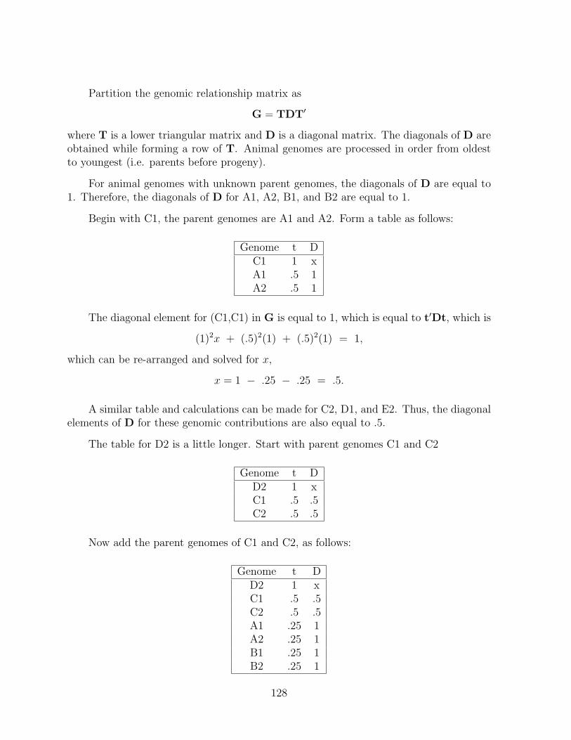
Partition the genomic relationship matrix as
G = TDT′
where T is a lower triangular matrix and D is a diagonal matrix. The diagonals of D areobtained while forming a row of T. Animal genomes are processed in order from oldestto youngest (i.e. parents before progeny).
For animal genomes with unknown parent genomes, the diagonals of D are equal to1. Therefore, the diagonals of D for A1, A2, B1, and B2 are equal to 1.
Begin with C1, the parent genomes are A1 and A2. Form a table as follows:
Genome t DC1 1 xA1 .5 1A2 .5 1
The diagonal element for (C1,C1) in G is equal to 1, which is equal to t′Dt, which is
(1)2x + (.5)2(1) + (.5)2(1) = 1,
which can be re-arranged and solved for x,
x = 1 − .25 − .25 = .5.
A similar table and calculations can be made for C2, D1, and E2. Thus, the diagonalelements of D for these genomic contributions are also equal to .5.
The table for D2 is a little longer. Start with parent genomes C1 and C2
Genome t DD2 1 xC1 .5 .5C2 .5 .5
Now add the parent genomes of C1 and C2, as follows:
Genome t DD2 1 xC1 .5 .5C2 .5 .5A1 .25 1A2 .25 1B1 .25 1B2 .25 1
128

The next step would be to add the ’parents’ of A1 and A2, then B1 and B2, but these’parents’ are unknown, and so no further additions to the table are made. Now computet′Dt as
x+ (.5)2(.5) + (.5)2(.5) + 4(.25)2(1) = 1,
orx = 1− .125− .125− 4(.0625) = .5.
The table of E1 is more complex. The parent genomes are D1 and D2. As the animalsbecome younger, the length of these tables can become greater, and with n generationsthere can be up to 2n + 1 elements in a table.
Genome t DE1 1 xD1 .5 .5D2 .5 .5A1 .25 1A2 .25 1C1 .25 .5C2 .25 .5A1 .125 1A2 .125 1B1 .125 1B2 .125 1
Note that A1 and A2 appear twice in the table. Their coefficients in t must be addedtogether before computing t′Dt. The new table, after adding coefficents is
Genome t DE1 1 xD1 .5 .5D2 .5 .5A1 .375 1A2 .375 1C1 .25 .5C2 .25 .5B1 .125 1B2 .125 1
Then
x = 1− 2(.5)2(.5)− 2(.375)2(1)− 2(.25)2(.5)− 2(.125)2(1) = .375.
The complete results for the diagonals of D are given in the next table.
129
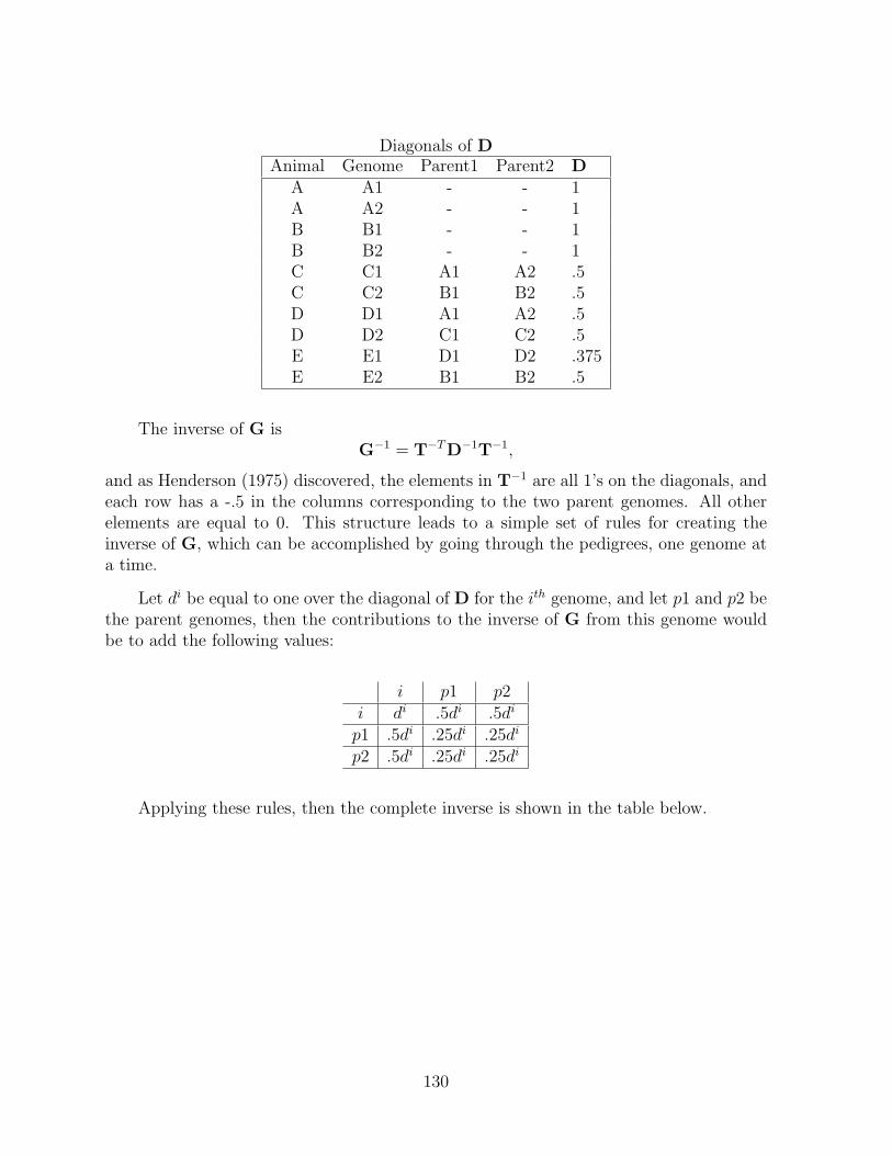
Diagonals of DAnimal Genome Parent1 Parent2 D
A A1 - - 1A A2 - - 1B B1 - - 1B B2 - - 1C C1 A1 A2 .5C C2 B1 B2 .5D D1 A1 A2 .5D D2 C1 C2 .5E E1 D1 D2 .375E E2 B1 B2 .5
The inverse of G isG−1 = T−TD−1T−1,
and as Henderson (1975) discovered, the elements in T−1 are all 1’s on the diagonals, andeach row has a -.5 in the columns corresponding to the two parent genomes. All otherelements are equal to 0. This structure leads to a simple set of rules for creating theinverse of G, which can be accomplished by going through the pedigrees, one genome ata time.
Let di be equal to one over the diagonal of D for the ith genome, and let p1 and p2 bethe parent genomes, then the contributions to the inverse of G from this genome wouldbe to add the following values:
i p1 p2i di .5di .5di
p1 .5di .25di .25di
p2 .5di .25di .25di
Applying these rules, then the complete inverse is shown in the table below.
130
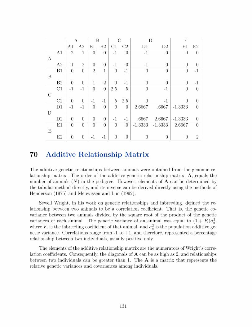
A B C D EA1 A2 B1 B2 C1 C2 D1 D2 E1 E2
A1 2 1 0 0 -1 0 -1 0 0 0A
A2 1 2 0 0 -1 0 -1 0 0 0B1 0 0 2 1 0 -1 0 0 0 -1
BB2 0 0 1 2 0 -1 0 0 0 -1C1 -1 -1 0 0 2.5 .5 0 -1 0 0
CC2 0 0 -1 -1 .5 2.5 0 -1 0 0D1 -1 -1 0 0 0 0 2.6667 .6667 -1.3333 0
DD2 0 0 0 0 -1 -1 .6667 2.6667 -1.3333 0E1 0 0 0 0 0 0 -1.3333 -1.3333 2.6667 0
EE2 0 0 -1 -1 0 0 0 0 0 2
70 Additive Relationship Matrix
The additive genetic relationships between animals were obtained from the genomic re-lationship matrix. The order of the additive genetic relationship matrix, A, equals thenumber of animals (N) in the pedigree. However, elements of A can be determined bythe tabular method directly, and its inverse can be derived directly using the methods ofHenderson (1975) and Meuwissen and Luo (1992).
Sewell Wright, in his work on genetic relationships and inbreeding, defined the re-lationship between two animals to be a correlation coefficient. That is, the genetic co-variance between two animals divided by the square root of the product of the geneticvariances of each animal. The genetic variance of an animal was equal to (1 + Fi)σ
2a,
where Fi is the inbreeding coefficient of that animal, and σ2a is the population additive ge-
netic variance. Correlations range from -1 to +1, and therefore, represented a percentagerelationship between two individuals, usually positive only.
The elements of the additive relationship matrix are the numerators of Wright’s corre-lation coefficients. Consequently, the diagonals of A can be as high as 2, and relationshipsbetween two individuals can be greater than 1. The A is a matrix that represents therelative genetic variances and covariances among individuals.
131

70.1 The Tabular Method
Additive genetic relationships among animals may be calculated using a recursive proce-dure called the Tabular Method (attributable to Henderson and perhaps to Wright beforehim). To begin, make a list of all animals that have observations in your data, and foreach of these determine their parents (called the sire and dam). An example list is shownbelow.
Animal Sire DamA - -B - -C - -D A BE A CF E D
The list should be in chronological order so that parents appear before progeny. Thesire and dam of animals A, B, and C are assumed to be unknown, and consequentlyanimals A, B, and C are assumed to be genetically unrelated. In some instances theparentage of animals may be traced for several generations, and for each animal theparentage should be traced to a common base generation.
Using the completed list of animals and pedigrees, form a two-way table with n rowsand columns, where n is the number of animals in the list, in this case n = 6. Label therows and columns with the corresponding animal identification and above each animal IDwrite the ID of its parents as shown below.
Tabular Method Example,Starting Values.
-,- -,- -,- A,B A,C E,DA B C D E F
A 1 0 0
B 0 1 0
C 0 0 1
D
E
F
132

For each animal whose parents were unknown a one was written on the diagonal ofthe table (i.e for animals A, B, and C), and zeros were written in the off-diagonals betweenthese three animals, assuming they were unrelated. Let the elements of this table (referedto as matrix A) be denoted as aij. Thus, by putting a 1 on the diagonals for animalswith unknown parents, the additive genetic relationship of an animal with itself is one.The additive genetic relationship to animals without common parents or whose parentsare unknown is assumed to be zero.
The next step is to compute relationships between animal A and animals D, E, andF. The relationship of any animal to another is equal to the average of the relationshipsof that animal with the parents of another animal. For example, the relationship betweenA and D is the average of the relationships between A and the parents of D, who are Aand B. Thus,
aAD = .5 ( aAA + aAB ) = .5(1 + 0) = .5aAE = .5 ( aAA + aAC ) = .5(1 + 0) = .5aAF = .5 ( aAE + aAD ) = .5(.5 + .5) = .5
The relationship table, or A matrix, is symmetric, so that aAD = aDA, aAE = aEA,and aAF = aFA. Continue calculating the relationships for animals B and C to give thefollowing table.
Tabular Method Example,Partially Completed.
-,- -,- -,- A,B A,C E,DA B C D E F
A 1 0 0 .5 .5 .5
B 0 1 0 .5 0 .25
C 0 0 1 0 .5 .25
D .5 .5 0
E .5 0 .5
F .5 .25 .25
Next, compute the diagonal element for animal D. By definition this is one plus theinbreeding coefficient, i.e.
aDD = 1 + FD.
133

The inbreeding coefficient, FD is equal to one-half the additive genetic relationship be-tween the parents of animal D, namely,
FD = .5aAB = 0.
When parents are unknown, the inbreeding coefficient is zero assuming the parents of theindividual were unrelated. After computing the diagonal element for an animal, like D,then the remaining relationships to other animals in that row are calculated as before.The completed matrix is given below. Note that only animal F is inbred in this example.The inbreeding coefficient is a measure of the percentage of loci in the genome of ananimal that has become homogeneous, that is, the two alleles at a locus are the same(identical by descent). Sometimes these alleles may be lethal and therefore, inbreeding isgenerally avoided.
Tabular Method ExampleCompleted Table.
-,- -,- -,- A,B A,C E,DA B C D E F
A 1 0 0 .5 .5 .5
B 0 1 0 .5 0 .25
C 0 0 1 0 .5 .25
D .5 .5 0 1 .25 .625
E .5 0 .5 .25 1 .625
F .5 .25 .25 .625 .625 1.125
Generally, the matrix A is nonsingular, but if the matrix includes two animals that areidentical twins, then two rows and columns of A for these animals would be identical, andtherefore, A would be singular. In this situation assume that the twins are geneticallyequal and treat them as one animal (by giving them the same registration number oridentification) (see Kennedy and Schaeffer, 1989).
71 Inbreeding Calculations
The inbreeding coefficients and the inverse of A for inbred animals are generally requiredfor BLUP analyses of animal models. Thus, fast methods of doing both of these calcula-tions, and for very large populations of animals are necessary.
134

A = TBT′,
where T is a lower triangular matrix and B is a diagonal matrix. Quaas (1976) showedthat the diagonals of B, say bii were
bii = (.5− .25(Fs + Fd)),
where Fs and Fd are the inbreeding coefficients of the sire and dam, respectively, of theith individual. If one parent is unknown, then
bii = (.75− .25Fp),
where Fp is the inbreeding coefficient of the parent that is known. Lastly, if neither parentis known then bii = 1.
One of the more efficient algorithms for calculating inbreeding coefficients is that ofMeuwissen and Luo (1992). Animals should be in chronological order, as for the TabularMethod. To illustrate consider the example given in the Tabular Method section. Thecorresponding elements of B for animals A to F would be(
1 1 1 .5 .5 .5).
Now consider a new animal, G, with parents F and B. The first step is to set up threevectors, where the first vector contains the identification of animals in the pedigree ofanimal G, the second vector will contain the elements of a row of matrix T, and the thirdvector will contain the corresponding bii for each animal.
Step 1 Add animal G to the ID vector, a 1 to the T-vector, and
bGG = .5− .25(.125 + 0) = 15/32
to the B-vector, giving
ID vector T-vector B-vectorG 1 15/32
Step 2 Add the parents of G to the ID vector, and because they are one generation back,add .5 to the T-vector for each parent. In the D-vector, animal B has bBB = 1, andanimal F has bFF = .5. The vectors now appear as
ID vector T-vector B-vectorG 1 15/32F .5 .5B .5 1
135

Step 3 Add the parents of F and B to the ID vector, add .25 (.5 times the T-vector valueof the individual (F or B)) to the T-vector, and their corresponding bii values. Theparents of F were E and D, and the parents of B were unknown. These give
ID vector T-vector B-vectorG 1 15/32F .5 .5B .5 1E .25 .5D .25 .5
Step 4 Add the parents of E and D to the ID vector, .125 to the T-vector, and theappropriate values to the B-vector. The parents of E were A and C, and the parentsof D were A and B.
ID vector T-vector B-vectorG 1 15/32F .5 .5B .5 1E .25 .5D .25 .5A .125 1C .125 1A .125 1B .125 1
The vectors are complete because the parents of A, B, and C are unknown and nofurther ancestors can be added to the pedigree of animal G.
Step 5 Accumulate the values in the T-vector for each animal ID. For example, animalsA and B appear twice in the ID vector. Accumulating their T-vector values gives
ID vector T-vector B-vectorG 1 15/32F .5 .5B .5+.125=.625 1E .25 .5D .25 .5A .125+.125=.25 1C .125 1
Do not accumulate quantities until all pathways in the pedigree have been processed,otherwise a coefficient may be missed and the wrong inbreeding coefficient could becalculated.
136

Step 6 The diagonal of the A matrix for animal G is calculated as the sum of the squaresof the values in the T-vector times the corresponding value in the B-vector, hence
aGG = (1)2(15/32) + (.5)2(.5) + (.625)2
+(.25)2(.5) + (.25)2(.5) + (.25)2 + (.125)2
= 72/64
= 11
8
The inbreeding coefficient for animal G is one-eighth.
The efficiency of this algorithm depends on the number of generations in each pedi-gree. If each pedigree is 10 generations deep, then each of the vectors above could haveover 1000 elements for a single animal. To obtain greater efficiency, animals with thesame parents could be processed together, and each would receive the same inbreedingcoefficient, so that it only needs to be calculated once. For situations with only 3 or 4 gen-eration pedigrees, this algorithm would be very fast and the amount of computer memoryrequired would be low compared to other algorithms (Golden et al. (1991), Tier(1990)).
71.1 Example Additive Matrix
Consider the pedigrees in the table below:
Animal Sire Dam1 - -2 - -3 1 -4 1 25 3 46 1 47 5 6
Animals with unknown parents may or may not be selected individuals, but theirparents (which are unknown) are assumed to belong to a em base generation of animals,i.e. a large, random mating population of unrelated individuals. Animal 3 has oneparent known and one parent unknown. Animal 3 and its sire do not belong to thebase generation, but its unknown dam is assumed to belong to the base generation. Ifthese assumptions are not valid, then the concept of phantom parent groups needs to beutilized (covered later in these notes). Using the tabular method, the A matrix for theabove seven animals is given below.
137

-,- -,- 1,- 1,2 3,4 1,4 5,61 2 3 4 5 6 7
1 1 0 .5 .5 .5 .75 .6252 0 1 0 .5 .25 .25 .253 .5 0 1 .25 .625 .375 .54 .5 .5 .25 1 .625 .75 .68755 .5 .25 .625 .625 1.125 .5625 .843756 .75 .25 .375 .75 .5625 1.25 .906257 .625 .25 .5 .6875 .84375 .90625 1.28125
Now partition A into T and B giving:
Sire Dam Animal 1 2 3 4 5 6 7 B1 1 0 0 0 0 0 0 1.02 0 1 0 0 0 0 0 1.0
1 3 .5 0 1 0 0 0 0 .751 2 4 .5 .5 0 1 0 0 0 .503 4 5 .5 .25 .5 .5 1 0 0 .501 4 6 .75 .25 0 .5 0 1 0 .505 6 7 .625 .25 .25 .5 .5 .5 1 .40625
Note that the rows of T account for the direct relationships, that is, the direct transferof genes from parents to offspring.
71.2 The Inverse of Additive Relationship Matrix
The inverse of the relationship matrix can be constructed similarly to the inverse of thegenomic relationship matrix by a set of rules. Recall the previous example of seven animalswith the following values for bii.
Animal Sire Dam bii b−1ii
1 - - 1.00 1.002 - - 1.00 1.003 1 - 0.75 1.333334 1 2 0.50 2.005 3 4 0.50 2.006 1 4 0.50 2.007 5 6 0.40625 2.4615385
Let δ = b−1ii , then if both parents are known the following constants are added to the
appropriate elements in the inverse matrix:
138

animal sire damanimal δ −.5δ −.5δsire −.5δ .25δ .25δdam −.5δ .25δ .25δ
If one parent is unknown, then delete the appropriate row and column from the rulesabove, and if both parents are unknown then just add δ to the animal’s diagonal elementof the inverse.
Each animal in the pedigree is processed one at a time, but any order can be taken.Let’s start with animal 6 as an example. The sire is animal 1 and the dam is animal 4. Inthis case, δ = 2.0. Following the rules and starting with an inverse matrix that is empty,after handling animal 6 the inverse matrix should appear as follows:
1 2 3 4 5 6 71 .5 .5 -1234 .5 .5 -156 -1 -1 27
After processing all of the animals, then the inverse of the relationship matrix forthese seven animals should be as follows:
1 2 3 4 5 6 71 2.33333 .5 -.66667 -.5 0 -1 02 .5 1.5 0 -1.00000 0 0 03 -.66667 0 1.83333 .5 -1 0 04 -.5 -1 .5 3.0000 -1 -1 05 0 0 -1 -1 2.61538 .61538 -1.230776 -1 0 0 -1 .61538 2.61538 -1.230777 0 0 0 0 -1.23077 -1.23077 2.46154
The product of the above matrix with the original relationship matrix, A, gives anidentity matrix.
71.3 R function To Construct A-inverse
Given a pedigree list and the corresponding bii values for each animal in the pedigree, thenthe inverse of A can be written. Below is a function in R that will do those calculations.Animals should be numbered consecutively from 1 to N .
139
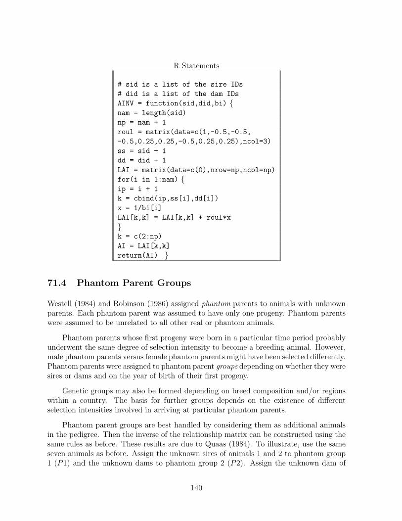
R Statements
# sid is a list of the sire IDs
# did is a list of the dam IDs
AINV = function(sid,did,bi) {nam = length(sid)
np = nam + 1
roul = matrix(data=c(1,-0.5,-0.5,
-0.5,0.25,0.25,-0.5,0.25,0.25),ncol=3)
ss = sid + 1
dd = did + 1
LAI = matrix(data=c(0),nrow=np,ncol=np)
for(i in 1:nam) {ip = i + 1
k = cbind(ip,ss[i],dd[i])
x = 1/bi[i]
LAI[k,k] = LAI[k,k] + roul*x
}k = c(2:np)
AI = LAI[k,k]
return(AI) }
71.4 Phantom Parent Groups
Westell (1984) and Robinson (1986) assigned phantom parents to animals with unknownparents. Each phantom parent was assumed to have only one progeny. Phantom parentswere assumed to be unrelated to all other real or phantom animals.
Phantom parents whose first progeny were born in a particular time period probablyunderwent the same degree of selection intensity to become a breeding animal. However,male phantom parents versus female phantom parents might have been selected differently.Phantom parents were assigned to phantom parent groups depending on whether they weresires or dams and on the year of birth of their first progeny.
Genetic groups may also be formed depending on breed composition and/or regionswithin a country. The basis for further groups depends on the existence of differentselection intensities involved in arriving at particular phantom parents.
Phantom parent groups are best handled by considering them as additional animalsin the pedigree. Then the inverse of the relationship matrix can be constructed using thesame rules as before. These results are due to Quaas (1984). To illustrate, use the sameseven animals as before. Assign the unknown sires of animals 1 and 2 to phantom group1 (P1) and the unknown dams to phantom group 2 (P2). Assign the unknown dam of
140

animal 3 to phantom group 3 (P3). The resulting matrix will be of order 10 by 10 :
A−1∗ =
(Arr Arp
Apr App
),
where Arr is a 7 by 7 matrix corresponding to the elements among the real animals; Arp
and its transpose are of order 7 by 3 and 3 by 7, respectively, corresponding to elementsof the inverse between real animals and phantom groups, and App is of order 3 by 3 andcontains inverse elements corresponding to phantom groups. Arr will be exactly the sameas A−1 given in the previous section. The other matrices are
Arp =
−.5 −.5 .33333−.5 −.5 0
0 0 −.666670 0 00 0 00 0 00 0 0
App =
.5 .5 0.5 .5 00 0 .33333
In this formulation, phantom groups (according to Quaas (1984)) are additional fixedfactors and there is a dependency between phantom groups 1 and 2. This singularitycan cause problems in deriving solutions for genetic evaluation. The dependency can beremoved by adding an identity matrix to App. When genetic groups have many animalsassigned to them, then adding the identity matrix to App does not result in any significantre-ranking of animals in genetic evaluation and aids in getting faster convergence of theiterative system of equations.
Phantom groups are used in many genetic evaluation systems today. The phantomparents assigned to a genetic group are assumed to be the outcome of non random matingand similar selection differentials on their parents. This assumption, while limiting, is notas severe as assuming that all phantom parents belong to one base population.
72 Identical Genotypes
Occasionally genetically identical twins are born, arising from a single embryo. Theseindividuals share all of the same genetic material, both nuclear and non-nuclear DNA. Inan additive genetic relationship matrix the rows for those two animals will be identical,and therefore, a dependency exists in the relationship matrix and an inverse is not possible.
Clones are individuals that tend to share only the nuclear DNA, and the assumptionis that the non-nuclear DNA can cause genetic and phenotypic differences between the
141

animals in their development. The additive genetic portion, which is passed on to progeny,is in the nuclear DNA, and therefore, the additive relationship matrix will have identicalrows of numbers for clones from the same animal. The additive relationship matrix wouldbe singular.
Kennedy and Schaeffer (1989) suggested that the relationship matrix be constructedfor “genotypes” rather than for individuals in the case of these identical animals. Ifthere were five clones of one animal, then the animal and its clones would represent onegenotype, and so there would be only one row of the additive relationship matrix for allsix animals. If the animals were measured for some trait, then that “genotype” wouldhave repeated observations (without permanent environmental effects). They would allreceive the same estimated breeding value.
One could also treat them as full-sibs, all having the same parents, but not sharingthe exact same DNA. If there were many of these in the data file, then it could cause anoverestimation of the additive genetic variance. Therefore, this approach would not besuitable.
73 Unknown Sires
In some situations a female is exposed to more than one possible mate. For example, agroup of cows in a beef herd may have access to 3 or 4 males during the breeding season.Another example occurs in mink breeding where the success of having conception requiresmating a female three times with different males at each mating. Progeny born from onefemale are a mixture of progeny of those three males. That is, different eggs could befertilized by different males. Through genetic tests, the probabilities that a progeny isfrom either the first, second, or third male are known.
The additive relationship matrix can be constructed using the probabilities that aspecific male is the sire of a given progeny. An example is as follows: Animals A and Bare males, C is a female, and D is a progeny of C with 0.25 probability that the sire wasA and 0.75 probability that the sire was B. Construct the additive genetic relationshipmatrix for this pedigree.
A B C DA 1 0 0 .125B 0 1 0 .375C 0 0 1 .5D .125 .375 .5 1
Normally the relationship of the sire to its progeny (if unrelated to the dam) is 0.5,but in this case, for the relationship between A and D, the value has to be multiplied
142

times the probability of A being the sire of D. Between B and D, the relationship of .5has to be multipled times .75.
The inverse of this matrix is derived in a similar manner as the regular additiverelationship matrix. The bi values for animals A, B, and C are equal to 1. Because D hastwo possible sires, its bi value needs to be calculated differently.
ID vector T-vector B-vectorD 1 xC .5 1B .375 1A .125 1
The diagonal of A for animal D has to be assumed to be known, as one plus one halfthe relationship between the sire(s) and dam. In this case, A, B, and C are all unrelated,and therefore, D will not be inbred, so that the diagonal of A will be 1.
aDD = 1 = x + (.5)2(1) + (.375)2(1) + (.125)2(1)
Solving for x gives .59375 = bD. The inverse elements added to A for animal D aregiven by
−.125−.375−.51
1
.59375
(−.125 −.375 −.5 1
)=
.0263 .0789 .1053 −.2105.0789 .2368 .3158 −.6316.1053 .3158 .4211 −.8421−.2105 −.6316 −.8421 1.6842
.
To complete the inverse, add 1 to the diagonals for animals A, B, and C.
74 EXERCISES
1. Use the following data for this problem.
Treatment Animal Sire Dam Observations1 1 152 2 731 3 442 4 1 3 561 5 2 4 552 6 1 5 611 7 6 4 322 8 7 5 47
143

Let the model equation be
yij = Ti + pj +mj + eij
where Ti is a fixed treatment effect, pj is a random, paternal gamete effect of animalj, mj is a random, maternal gamete effect of animal j, and eijk is a random, residualeffect. Assume that
σ2e = 3.2σ2
G.
(a) Complete the genomic relationship matrix for the eight animals, and the inverseof it.
(b) Construct the MME and solve.
(c) Predict the breeding values of each animal and obtain the standard errors ofprediction.
(d) Test the difference between the treatments.
(e) Form the additive relationship matrix for this pedigree.
(f) Calculate the inverse of A.
(g) Assume the modelyij = Ti + aj + eij
where aj is the animal additive genetic effect with covariance matrix Aσ2a, and
whereσ2e = 1.6σ2
a.
Construct the MME for this model and solve. Compare EBVs from this modeland the previous model.
2. Use the following data for this problem.
Animal Sire Dam CG Observations1234 1 3 1 65 2 4 1 156 1 1 97 2 6 2 118 1 3 2 89 2 4 2 1310 5 8 3 711 5 3 3 1012 2 7 3 5
144

Let the model equation beyij = CGi + aj + eij
where CGi is a fixed contemporary group effect, aj is a random, animal additivegenetic effect, and eijk is a random residual effect. Assume that
σ2e = 1.2 σ2
a.
(a) Complete the additive relationship matrix and the inverse of it.
(b) Construct the MME and solve for this model.
(c) Compute SEP for the EBV and also reliabilities.
3. You are given the following pedigree information and values of bi. Determine the bivalue and inbreeding coefficient of animal H which is a progeny of animals G and F.
Animal Sire Dam Fi biA 0 1B A 0 3/4C A B 1/4 1/2D C B 3/8 7/16E A D 5/16 13/32F C D 1/2 11/32G E B 11/32 27/64H G F
Write out A−1 for this pedigree using Henderson’s rules.
4. The following boxes are from a larger genomic relationship matrix.
L KKm Kf Lm Lf Mm Mf
Gm 12
0 14
38
w x
Gf 14
12
12
18
y z
(a) Calculate w, x, y, and z.
(b) Calculate aGL and dGL
5. Assign phantom groups to replace missing sire and dam identifications in the fol-lowing pedigree.
145
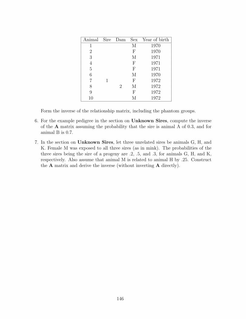
Animal Sire Dam Sex Year of birth1 M 19702 F 19703 M 19714 F 19715 F 19716 M 19707 1 F 19728 2 M 19729 F 197210 M 1972
Form the inverse of the relationship matrix, including the phantom groups.
6. For the example pedigree in the section on Unknown Sires, compute the inverseof the A matrix assuming the probability that the sire is animal A of 0.3, and foranimal B is 0.7.
7. In the section on Unknown Sires, let three unrelated sires be animals G, H, andK. Female M was exposed to all three sires (as in mink). The probabilities of thethree sires being the sire of a progeny are .2, .5, and .3, for animals G, H, and K,respectively. Also assume that animal M is related to animal H by .25. Constructthe A matrix and derive the inverse (without inverting A directly).
146

Phantom Parent Groups
75 Background History
Pedigree information on each animal may not be traceable back to the same base genera-tion due to lack of recording and/or movement of animals from one owner to another (inthe same or different countries). Therefore, a pedigree file may have many animals withmissing parent identification. Animals with missing parents should not be assumed to befrom a homogeneous base population.
One technique to deal with missing parent information is to assign a parent groupto an animal based upon the year of birth of the animal and the pathway of selection. Ifthe animal is a female, for example, and the dam information is missing, then the parentgroup would be in the Dams of Females pathway (DF). There are also Dams of Males(DM), Sires of Females (SF), and Sires of Males (SM). Four pathways and various years ofbirth nested within each pathway. These have become known as phantom parent groups.
Genetic group effects are added to the model.
y = Xb + ZQg + Za + e,
where
a is the vector of animal additive genetic effects,
Z is the matrix that relates animals to their observations,
g is the vector of genetic group effects, and
Q is the matrix that relates animals to their genetic groups, and
y,Xb, e are as described in earlier notes.
The Estimated Breeding Value, EBV, of an animal is equal to the sum of the group andanimal solutions from MME, i.e.
Vector of EBVs = Qg + a.
The grouping strategy described above was developed by Westell (1988), Quaas(1988),and Robinson(1986). To illustrate, phantom parents have been added to the followingpedigrees, indicated by P1 to P6.
147

Animal Sire DamA P1 P4B P2 P5C P3 P6D A BE A CF E D
Now assign P1, P2, and P3 to genetic group 1 and P4, P5, and P6 to genetic group2. The pedigree list becomes
Animal Sire DamA G1 G2B G1 G2C G1 G2D A BE A CF E D
75.1 Simplifying the MME
The advantage of phantom parent grouping is that the mixed model equations simplifysignificantly. Using the previous model, the MME are X′X X′ZQ X′Z
Q′Z′X Q′Z′ZQ Q′Z′ZZ′X Z′ZQ Z′Z + A−1α
b
ga
=
X′yQ′Z′yZ′y
.Notice that Q′ times the third row subtracted from the second row gives
Q′A−1aα = 0.
Quaas and Pollak (1981) showed that the above equations could be transformed so thatQg + a can be computed directly. The derivation is as follows. Note that b
ga
=
I 0 00 I 00 −Q I
I 0 0
0 I 00 Q I
b
ga
=
I 0 00 I 00 −Q I
b
gQg + a
.
148

Substituting this equality into the left hand side (LHS) of the MME gives X′X 0 X′ZQ′Z′X 0 Q′Z′ZZ′X −A−1Qα Z′Z + A−1α
b
gQg + a
=
X′yQ′Z′yZ′y
.To make the equations symmetric again, both sides of the above equations must bepremultiplied by I 0 0
0 I −Q′
0 0 I
.This gives the following system of equations as X′X 0 X′Z
0 Q′A−1Qα −Q′A−1αZ′X −A−1Qα Z′Z + A−1α
b
gQg + a
=
X′y0
Z′y
.Quaas (1988) examined the structure of Q and the inverse of A under phantom parentgrouping and noticed that Q′A−1Q and −Q′A−1 had properties that followed the rulesof Henderson (1976) for forming the elements of the inverse of A. Thus, the elements ofA−1 and Q′A−1Q and −Q′A−1 can be created by a simple modification of Henderson’srules. Use δi as computed earlier, (i.e. δi = B−1
ii ), and let i refer to the individual animal,let s and d refer to either the parent or the phantom parent group if either is missing,then the rules are
Constant to Add Location in Matrixδi (i, i)−δi/2 (i, s),(s, i),(i, d), and (d, i)δi/4 (s, s),(d, d),(s, d), and (d, s)
Thus, Q′A−1Q and Q′A−1 can be created directly without explicitly forming Q andwithout performing the multiplications times A−1.
75.2 Typical Computational Problems
The solution to the modified equations has a problem in that the genetic group effects arestill fixed effects and some restriction on their solutions may be needed to reach conver-gence. For animals with both parents unknown, then there can be complete confoundingbetween the sire parent group and the dam parent group which causes a problem in gettinga solution. Kennedy proposed to break confounding by defining genetic groups such thatsire parent groups might be 70-71, 72-73, etc., while dam parent groups might be 69-70,71-72, 73-74, etc. giving an overlap between sire and dam groups. Schaeffer (personalpractice) suggested adding α to the diagonals of the genetic group effect equations inthe modified equations. This automatically removes confounding, and the genetic groupsolutions sum to zero.
149

76 Estimation of Variances
A simulation study was conducted to look at the effects of genetic grouping methods, ingeneral. A base population of 100 sires and 2000 dams was generated. Matings withina generation were random. Each mating resulted in one offspring, hence 2000 offspringper generation. Two correlated traits were simulated for each animal with a geneticcorrelation of 0.10, and a residual correlation of 0.30. Selection of males and femalesfor the next generation was on the basis of trait 2 phenotypes (available for males andfemales). Animals were selected across generations, and so generations were overlapping.Trait 1 was analyzed in this study and only females after generation 0 were assumed tohave single records for trait 1. The residual and genetic variances for both traits werethe same. Total phenotypic variance was 100, and heritability in the base population was0.25. Eight generations of selection and matings were made after the base population.Complete pedigrees were known in this population, denoted as P0. No phantom groupingwas necessary with this population because all animals traced back to the same basepopulation parents.
Two subpopulations were created from P0 by randomly eliminating parents of an-imals. Two different percentages were utilized, being 10 and 25%, denoted as P10 andP25, respectively. Different rates were used to test the impact on EBVs and genetic pa-rameters. Phantom parent groups were formed according to the four pathways of selectionand by generation of birth, i.e. 32 groups. There were no attempts to ensure a particularnumber of animals per group, but on average there would be 50 per group at 10% and125 at 25%. The unknown parents, however, have an effect on the inbreeding coefficients,and therefore, on the elements in the relationship matrix inverses.
77 Models of Analyses
Several different models were applied to each data set.
77.1 Model 1
A simple animal model was assumed where
y = 1µ+ Za + e,
where y are the trait 1 single records on females, µ is the overall mean, a is the vector ofanimal additive genetic effects for all males and females in the population, and e is thevector of residual effects. Also,
V ar(a) = Aσ2a,
150

where A−1 was created from the pedigree that was known in a given population. Thismodel assumes all animals can be traced back to the same base population animals.
77.2 Model 2
Due to selection there are usually time trends that need to be taken into account. This isaccomplished by adding a generation effect to the model replacing the overall mean effect.This is also a form of genetic grouping where Q denotes to which group each animal witha record belongs, and X = ZQ.
y = Xb + Za + e,
where b are the 8 generation effects. Phantom parent groups are not utilized with thismodel. The EBVs of animals with records is the sum of the generation group solutionplus the additive genetic solution.
77.3 Model 3
The model isy = 1µ+ ZQg + Za + e,
where Q describes the phantom parent grouping definitions, and g are the phantom groupeffects. With this model the phantom group effects can be either fixed or random. Thismodel and model 4 were only applied to populations P10 and P25. EBVs were obtaineddirectly from this model (Qg + a).
77.4 Model 4
The model isy = Xb + ZQg + Za + e,
which has generation effects in b and also uses phantom grouping in g. The definition ofan EBV is not clear in this model. There is double counting for genetic trend in b and ing. The EBV was the sum of the generation group solution and the animal solution.
78 Analyses
Fifty (50) replicates were made of each population structure and model of analysis. Vari-ance components were estimated using Bayesian methods and Gibbs sampling (30,000total samples and 3,000 burn-in period).
151

EBVs were calculated in the next step using the estimated components, using a setconvergence criteria or a maximum of 3000 iterations, whichever came first. No restrictionswere placed on any solutions. Iteration on data methods were used to solve the MME.Average inbreeding coefficients by generation were summarized. Correlations of EBVswith true breeding values were computed for all animals in generations 1 to 8. Truegenetic trends in males and females by generation were averaged over replicates. Thedifference between true generation average and estimated average in generation 8 wasused to determine if trends were under or over estimated.
Note that when phantom groups were fixed, there were severe confounding problemswith the MME, and therefore, only results for when the variance ratio (residual to genetic)was added to the diagonals of the phantom group equations are reported here(i.e. whenphantom groups were random). The correlations between true and estimated breedingvalues for fixed phantom groups were less than 0.2 with Model 3, for example.
79 Results
Table 1 gives the correlations between true and estimated breeding values of all animalsfrom generations 1 to 8. The best model appears to be one without any generationeffects or phantom groups, for all pedigree structures. As the percentage of animalswith unknown parents is increased the correlation decreases. Differences between modelsand pedigree structures were significantly different from Model 1 and P0. Although thedifferences are significant statistically, they may not be practically significant.
Table 1Correlations of true breeding values withestimated breeding values of all animals
from generations 1 to 8.Standard error of estimates was 0.0025.
Data Model 1 Model 2 Model 3 Model 4Set µ Xb µ+ ZQg Xb + ZQg
P0 .588 .579
P10 .575 .567 .567 .568
P25 .555 .550 .544 .547
Average inbreeding coefficients of animals born in generation 8 are given in Table2. When full pedigree information was available back to the base population, then theaverage inbreeding coefficient was 0.00872. When 10% of the parents were assumed to
152

be unknown the average inbreeding coefficient dropped by about 0.0027 (which was sta-tistically significant), and at 25% a drop of 0.0054 occurred. Thus, inbreeding rate issignificantly underestimated when pedigrees are missing. The differences are small on apractical basis, but over time these differences would become greater.
Table 2Average inbreeding coefficients computed from
known pedigree information of animals ingeneration 8.
Standard error of estimates was 0.000001.Data Model 1 Model 2 Model 3 Model 4Set µ Xb µ+ ZQg Xb + ZQg
P0 .00872 .00872
P10 .00596 .00594 .00585 .00587
P25 .00330 .00328 .00325 .00322
Estimates of genetic and residual variances and heritability are given in Table 3.Model 1 was unbiased for all three pedigree structures, as was Model 3 for P10 and P25.Thus, phantom parent groups may be ignored when estimating genetic parameters underany pedigree structure. Including a fixed generation effect in the model tended to bias thegenetic component downwards and resulted in underestimated heritability. The residualcomponent was not affected.
Table 3Estimates of genetic (G) and residual (R)
variances and heritability (h2).Standard errors of estimates were 0.60, 0.71,
and 0.006 for R, G, and h2, respectively.
153

Data Model 1 Model 2 Model 3 Model 4Set µ Xb µ+ ZQg Xb + ZQg
P0 R 74.8 75.5G 25.1 24.2h2 .251 .242
P10 R 74.8 75.7 74.9 75.4G 25.3 23.8 25.4 24.2h2 .252 .239 .252 .243
P25 R 74.9 75.9 74.9 75.4G 25.2 23.5 25.3 24.2h2 .251 .236 .252 .242
Genetic trends were also affected by the model and pedigree structure. The averagedifferences between true genetic averages and estimated genetic averages in generation 8are shown in Table 4. Model 1 (with no generation effects or phantom groups) alwaysunderestimated the true genetic change in the population. The bias increased as thepercentage of unknown parents increased. Model 3 (with phantom parent groups) wasalso underestimated, but not as much as Model 1. When generation effects were in themodel (Models 2 and 4), then genetic trends were estimated unbiasedly.
Table 4Average difference of true minus estimatedgenetic averages of animals in generation 8,
expressed in genetic standard deviation units.Standard error of estimates was 0.008.
Data Model 1 Model 2 Model 3 Model 4Set µ Xb µ+ ZQg Xb + ZQg
P0 .187 -.004
P10 .274 -.005 .233 .007
P25 .361 -.005 .246 .010
Table 5 shows trends in phantom group solutions for Model 3 as fixed or random,averaged over replicates, and also shows true genetic trends for comparison and estimatesof generation effects from Model 2. Phantom group solutions did not follow true genetictrends (either as fixed or as random), and there is no theoretical requirement anywherethat the phantom group solutions should be smooth or linear. When phantom groups are
154

fixed, the estimates had much higher standard errors, and were too variable from replicateto replicate. The generation effect estimates from Model 2 were linear and smooth, butunderestimated the true genetic trend. However, when the generation effect solutions areadded to the animal solutions to give EBV, the trend in average EBV gives an unbiasedestimate of the true genetic trend.
Table 5Two sets of phantom group solutions for Model 3,
P10, for fixed and random analysis, averageestimates of generation effects from Model 2,
and average true breeding values by generation.
Gen. True b SB SC DB DC1 -.044 .006 .093 -1.220 .730 -.580 R
2.526 -1.448 2.408 -.590 F2 .661 .530 .276 .447 .714 .079 R
-5.268 .780 6.311 .175 F3 1.041 .930 .762 -.450 1.202 .407 R
3.295 -.472 -.469 .589 F4 1.426 1.219 .968 1.948 1.300 1.302 R
1.892 2.743 3.443 1.682 F5 1.841 1.625 1.072 1.558 1.172 1.086 R
-1.974 2.206 3.455 1.401 F6 2.220 1.996 1.518 1.457 1.704 1.467 R
-2.589 2.116 4.278 1.885 F7 2.665 2.301 .855 1.875 .647 1.592 R
-1.505 2.690 -7.416 2.021 F8 3.006 2.668 .003 2.150 .005 1.921 R
.000 3.087 .000 2.492 FSE .099 .373 .373 .373 .373 R
2.366 2.366 2.366 2.366 F
80 Discussion and Conclusions
Limitations of this study were
1. Missing parents were determined randomly for lack of knowledge about how missingparents are actually sampled. Thus, if parents are missing based on some selectivestrategy, then the results could be much worse than shown here for P10 and P25.
2. Selection in this simulation on phenotypes of trait 2, while analyzing only trait 1in females was a simplification as might occur when analyzing fertility traits, forexample, after selection for many generations on production.
155

3. Phenotypic selection would keep inbreeding from accumulating too quickly in thissmall population.
4. Assortative mating of parents would be another complication to this simulation thatwould likely increase inbreeding, as well as genetic change.
5. Results may also differ slightly with heritability of the trait.
The choice of model seems to depend on the objective of the analysis. If the objectiveis to estimate the genetic parameters unbiasedly, then Model 1 should be used. However,Model 1 significantly underestimates genetic trends. The best model for estimation ofgenetic trend was Model 2. The degree of underestimation by Model 1 depends on thepercentage of missing parent information. Thus, the best course of action seems to be touse Model 1 for estimating parameters, and with those parameter estimates use Model 2to get unbiased estimates of genetic trend and presumably EBVs. Hence, phantom parentgroups are not necessary for either objective. Models 3 and 4 gave lower correlations oftrue BV with EBV than Models 1 or 2.
If phantom parent groups are used, then do not expect the solutions to be smoothand linear, or to follow the true genetic trend. Forcing phantom group solutions to besmooth would be incorrect and could introduce bias to EBVs. Phantom groups as randomshould be better than phantom groups as fixed, but there have been other studies thathave shown no differences between fixed or random if the number of animals per phantomgroup is large.
156

Animal Model
81 Introduction
In animal genetics, measurements are taken on individual animals, and thus, the modelof analysis should include the animal additive genetic effect. The remaining items in themodel are factors that have an effect on the trait of interest. The infinitesimal geneticmodel is assumed, and the animals that have been measured should represent a randomsample (or the entire sample) of progeny of the breeding males and females in the popu-lation. That means measurements should not be taken only from the biggest progeny, orthe best progeny, or the poorest progeny, but a random sample of progeny.
A simple animal model with one record per animal is
yi = µ + ai + ei,
where yi is the phenotypic record or observation, µ is the overall mean of the observations,ai are the additive genetic values of animals, and ei are the residual or environmentaleffects associated with the ith observation. Assumptions for this model are
1. The population is large (infinite) in size.
2. The association of alleles from the two parents is assumed to be at random.
3. No selection has been imposed on individual records.
4. Only additive genetic effects exist.
5. The influence of other factors on the observations is absent.
The expectations (for the example data to follow) are
E(ai) = 0, and E(ei) = 0,
and the variances are
V ar(ai) = σ2a,
V ar(ei) = σ2e .
The variances are assumed known, at least to proportionality. The covariance matrix ofthe vector of animal additive genetic effects is
V ar(a) = Aσ2a.
157

The relationship matrix is assumed to be complete back to the base population ( a large,randomly mating population ).
The heritability of the trait is
h2 =σ2a
σ2a + σ2
e
,
and the ratio of variances is
α =σ2e
σ2a
.
82 Example Problem
Below is the pedigree information and data on 16 animals. The first four animals werebase generation animals without records.
82.1 Data
Animal Sire Dam Record Animal Sire Dam Record1 0 0 9 5 6 36.02 0 0 10 7 8 66.43 0 0 11 5 8 28.94 0 0 12 7 6 73.05 1 2 38.5 13 1 6 44.26 3 4 48.9 14 3 8 53.47 3 2 64.3 15 5 4 33.68 1 4 50.5 16 7 8 49.5
The number of observations is N = 12, and the total sum of squares is 30, 811.78.Let σ2
a = 36, and σ2e = 64, so that h2 = 0.36, and α = 1.777778.
158

82.2 Additive Genetic Relationships
The matrix of additive genetic relationships among the sixteen individuals is A (times16) given below:
16 0 0 0 8 0 0 8 4 4 8 0 8 4 4 40 16 0 0 8 0 8 0 4 4 4 4 0 0 4 40 0 16 0 0 8 8 0 4 4 0 8 4 8 0 40 0 0 16 0 8 0 8 4 4 4 4 4 4 8 48 8 0 0 16 0 4 4 8 4 10 2 4 2 8 40 0 8 8 0 16 4 4 8 4 2 10 8 6 4 40 8 8 0 4 4 16 0 4 8 2 10 2 4 2 88 0 0 8 4 4 0 16 4 8 10 2 6 8 6 84 4 4 4 8 8 4 4 16 4 6 6 6 4 6 44 4 4 4 4 4 8 8 4 16 6 6 4 6 4 88 4 0 4 10 2 2 10 6 6 18 2 5 5 7 60 4 8 4 2 10 10 2 6 6 2 18 5 5 3 68 0 4 4 4 8 2 6 6 4 5 5 16 5 4 44 0 8 4 2 6 4 8 4 6 5 5 5 16 3 64 4 0 8 8 4 2 6 6 4 7 3 4 3 16 44 4 4 4 4 4 8 8 4 8 6 6 4 6 4 16
.
82.3 Application of BLUP with R
The construction of mixed model equations begins by defining X, Z, G and R.
X is a vector of ones of order 12 by 1.
Z is a 12 by 16 matrix, in which the first four columns are all zero, and the last 12columns are an identity matrix.
G is Aσ2a of order 16, and
R is Iσ2e of order 12.
To set up X in R, use the jd function below.
# function to form a J matrix - all ones
jd <- function(n,m) matrix(c(1),nrow=n,ncol=m)
X = jd(12,1)
There are at least two ways to create Z.
159

# First Method
# function to make an identity matrix
id <- function(n) diag(c(1),nrow=n,ncol=n)
Z = cbind((jd(12,4)*0),id(12))
# Second Method
# function to make a design matrix
desgn <- function(vnum) {mrow = length(vnum)
mcol = max(vnum)
W = matrix(data=c(0),nrow=mrow,ncol=mcol)
for(i in 1:mrow) {ic = vnum[i]
W[i,ic] = 1 }return(W) }
anim = c(5:16) # animals with records
Z = desgn(anim)
The desgn function can be used generally for creating design matrices from a list ofthe levels of a factor.
The inverse of the relationship matrix is needed. A list of the sires and dams of the16 animals are needed, with zeros for missing parents, and a list of the bi values for eachanimal are needed. In this example, the bis for animals 1 to 4 are 1, and for animals 5through 16 are 0.5.
160

y = matrix(data=c(38.5,48.9,64.3,50.5,36.0,66.4,28.9,
73.0,44.2,53.4,33.6,49.5)
bii = c(1,1,1,1,.5,.5,.5,.5,.5,.5,.5,.5,.5,.5,.5,.5)
sid = c(0,0,0,0,1,3,3,1,5,7,5,7,1,3,5,7)
did = c(0,0,0,0,2,4,2,4,6,8,8,6,6,8,4,8)
AI = AINV(sid,did,bii)
# multiply AI by the variance ratio
GI = AI * alpha
RI = id(12)
Alpha is the ratio of residual to additive genetic variances. In this example, the ratiois 64 divided by 36, or 1.778. The last line above creates the inverse of R which is anidentity matrix. Finally, the mixed model equations are created and solved using the MME
function given in an earlier section of the notes.
Exmp = MME(X,Z,GI,RI,y)
Exmp$LHSExmp$RHSExmp$CExmp$SOLNS
82.4 Solutions and SEP
The solutions for the animals are given in the next table. The estimate of the overallmean was 48.8955.
EBV for animals from MME and diagonals of the inverseof the LHS.
161

Animal EBV Diagonals1 -4.7341 .48662 .3728 .49593 5.8579 .47864 -1.4967 .4975
5 -7.1305 .41986 2.1335 .42607 8.4380 .41378 -2.1543 .42749 -4.7807 .4592
10 6.2947 .458211 -8.0126 .479512 9.4167 .475113 -2.0456 .450714 2.4341 .450115 -6.7242 .445916 2.5849 .4582
An estimate of the residual variance is obtained by subtracting the total sum ofsquares minus the sum of squares due to the model, and dividing that by N − r(X).
SST = 30, 811.78
SSR = 29, 618.3158
SST − SSR = 1193.464
σ2e = 108.4967
The Standard Error of Prediction (SEP) of an Estimated Breeding Value (EBV) isthe square root of the product of the diagonal of the inverse of the LHS times the estimateof residual variance. Thus for animal 1 in the table above, the SEP is
SEP = (.4866× 108.4967).5 = 7.2662.
82.5 Reliability
The reliability (REL) of an EBV is another measure of accuracy of the estimate.
RELi = (aii − ciiα)/aii,
where aii is the diagonal of the A matrix for animal i, and cii is the diagonal of the inverseof the LHS (in the table above). For animal 1,
REL = (1 − .4866(1.778))/1 = .1349.
162

The reliability is only 13.49 %, which is low.
Publication of “official” EBV often requires a minimum reliability, such as 75%, plusminimums on number of progeny and number of contemporary groups for those progeny.
83 Simulation of Records
The sampling processes involved in generating a set of data are better understood throughsimulation.
83.1 Generating Breeding Values of Animals
Let the heritability of the trait be 0.25, and the variance of phenotypic records to be 100.Then, σ2
a = 25, and σ2e = 75. Breeding values of base population animals are created by
multiplying a pseudo-random normal deviate, RND, times the genetic standard deviation,σa = 5. Let there be two base animals,
a1 = −1.8014 ∗ 5 = −9.0070
a2 = 0.6556 ∗ 5 = 3.2780
Progeny can be generated from animals previously generated as the average of theparent breeding values plus a Mendelian sampling effect. The Mendelian sampling effectis the product of another random normal deviate times the genetic standard deviation ofthe Mendelian sampling effect. The variance of the Mendelian sampling effect is bi timesthe genetic variance, where bi is obtained during the calculation of inbreeding coefficients(given in previous notes). That is,
bi = (0.5− 0.25 ∗ (Fs + Fd)),
where Fs and Fd are the inbreeding coefficients of the sire and dam, respectively.
Let Animal 3 be a progeny of animals 1 and 2,
a3 = 0.5 ∗ (a1 + a2) + m3
b3 = 0.5,
m3 = (0.5).5σa RND
= 0.7071 ∗ 5 ∗ (−.4045),
= −1.4301
163

a3 = 0.5(−9.0070 + 3.2780)− 1.4301
= −4.2946.
83.2 Phenotypic Records
To create phenotypic records, the equation of the model must be specified. Assume that
yij = µ + dj + ai + eij,
where µ is an overall mean (assume a value of 50); dj is a diet effect for one of 3 diets, aiis the animal breeding value, and eij is a residual effect.
Animals must be assigned to a diet. One way is to have the experimental designknown in advance, such that an animal is created for a specific diet. Another way is topick one of the three diets randomly and assign it to that animal. The differences amongthe diets should be set before generating records. Assume that
d1 = −10.0,
d2 = 0,
d3 = 10.0.
Diet differences would be constant for all animals generated. If the simulation wererepeated, then the same differences would probably be used. This would be the tradition-alist’s view of a fixed factor.
Residual effects are random and specific to each observation. A residual effect isgenerated by multiplying a random normal deviate times the residual standard deviation.
A record for animal 3, in diet 3, would be
y33 = 50 + 10.0 − 4.2946 + .3939(8.6602) = 59.1167.
Usually observations will be to the nearest whole number, so that y33 = 59 would be thefinal result for animal 3.
If animals are generated in chronological order, then inbreeding coefficients need to becalculated as new animals are generated, so that bi values can be obtained for generatingMendelian sampling effects. This is an efficient algorithm for simulating data for largepopulations. A later set of notes will consider using R to generate large populations ofanimals for single or multiple traits.
84 Measuring Genetic Change
To measure genetic change, the population needs to be defined precisely. In dairy cattle,one population would be all females born, by year of birth. Then the average EBVs of
164

cows by year of birth would estimate the genetic change in new females coming into thepopulation.
Another population could be all females calving in a particular year. This is differentfrom the first population because cows can have several calvings over their lifetime, andsecondly not all females that are born would necessarily calve even once. A cow’s EBVcould appear in the calculations in more than one year of calving. This would representthe trend in genetic merit of actively lactating cows.
In beef cattle, the averages for females being bred in a given year could be an inter-esting trend to monitor versus the average of females that produce a calf. In all cases,EBVs are used in the calculations.
Genetic trends can be overestimated if the heritability used in the calculation ofEBV is too large. Similarly, if the heritability is too low, then genetic trend can beunderestimated. Thus, having good estimates of the variance parameters is crucial togood estimates of genetic trend.
85 Reduced Animal Models
85.1 Usual Animal Model Approach
Consider an animal model with periods as a fixed factor and one observation per animal,as in the table below.
Animal Model Example DataAnimal Sire Dam Period Observation
5 1 3 2 2506 1 3 2 1987 2 4 2 2458 2 4 2 2609 2 4 2 2354 - - 1 2553 - - 1 2002 - - 1 225
Assume that the ratio of residual to additive genetic variances is 2. The MME forthis data would be of order 11 (nine animals and two periods).
165

3 0 0 1 1 1 0 0 0 0 00 5 0 0 0 0 1 1 1 1 10 0 4 0 2 0 −2 −2 0 0 01 0 0 6 0 3 0 0 −2 −2 −21 0 2 0 5 0 −2 −2 0 0 01 0 0 3 0 6 0 0 −2 −2 −20 1 −2 0 −2 0 5 0 0 0 00 1 −2 0 −2 0 0 5 0 0 00 1 0 −2 0 −2 0 0 5 0 00 1 0 −2 0 −2 0 0 0 5 00 1 0 −2 0 −2 0 0 0 0 5
b1b2a1
a2
a3
a4
a5
a6
a7
a8
a9
=
6801188
0225200255250198245260235
and the solutions to these equations are
b1b2a1
a2
a3
a4
a5
a6
a7
a8
a9
=
225.8641236.3366−2.4078
1.3172−10.2265
11.3172−2.3210−12.7210
6.78649.78644.7864
.
Some species, such as swine or rainbow trout, have many offspring per mating, andsubsequently fewer animals are needed for breeding purposes. The MME would containmany equations (one per animal), even though a large percentage of animals do not haveany progeny. Reducing the order of the MME would be an advantage, to save computingtime. Quaas and Pollak (1980) proposed the reduced animal model. There is one modelfor animals that are not parents, and a separate model for animals that are parents. Thetotal number of animal genetic equations in MME is equal to the number of animals thatare parents. The solutions for the animals in the reduced animal model are exactly thesame as solutions from the regular animal model.
85.2 Theoretical Development
The vector of additive genetic values of animals in the animal model is a. Denote animalswith progeny as ap, and those without progeny as ao, so that
a′ =(
ap′ ao
′).
166

In terms of the example data,
ap′ =
(a1 a2 a3 a4
),
ao′ =
(a5 a6 a7 a8 a9
).
The additive genetic value of an animal may be written as the average of the additivegenetic values of the parents plus a Mendelian sampling effect, which is the animal’sspecific deviation from the parent average, i.e.
ai = .5(as + ad) +mi.
Therefore,ao = Pap + m,
where P is a matrix that indicates the parents of each animal in ao, with elements equalto 0.5, and m is the vector of Mendelian sampling effects. Then
a =
(apao
)
=
(IP
)ap +
(0m
),
and
V ar(a) = Aσ2a
=
(IP
)App
(I P′
)σ2a +
(0 00 D
)σ2a
where D is a diagonal matrix with diagonal elements equal to bi, and bi is 0.5 − 0.25 ∗(Fs + Fd) for the ith animal, and
V ar(ap) = Appσ2a.
The animal model can now be written as(ypyo
)=
(Xp
Xo
)b +
(Zp 00 Zo
)(IP
)ap +
(ep
eo + Zom
).
The residual vector has two types of residuals and the additive genetic values of animalswithout progeny have been replaced with Pap. Because every individual has only onerecord, then Zo = I, but Zp may have fewer rows than there are elements of ap becausenot all parents may have observations themselves. In the example data, animal 1 doesnot have an observation, therefore,
Zp =
0 1 0 00 0 1 00 0 0 1
.167

Consequently,
R = V ar
(ep
eo + m
)
=
(Iσ2
e 00 Iσ2
e + Dσ2a
)
=
(I 00 Ro
)σ2e
The mixed model equations for the reduced animal model are(X′pXp + X′oR
−1o Xo X′pZp + X′oR
−1o P
Z′pXp + P′R−1o Xo Z′pZp + P′R−1
o P + A−1pp α
)(bap
)
=
(X′pyp + X′oR
−1o yo
Z′pyp + P′R−1o yo
).
Solutions for ao are derived from the following formulas:
ao = Pap + m,
wherem = (Z′oZo + D−1α)−1(yo −Xob−Pap).
85.3 Analysis of Example Data
Using the example data,
P =
.5 0 .5 0.5 0 .5 00 .5 0 .50 .5 0 .50 .5 0 .5
,
andD = diag
(.5 .5 .5 .5 .5
),
then the MME with α = 2 are
3 0 0 1 1 10 4 .8 1.2 .8 1.20 .8 2.4 0 .4 01 1.2 0 3.6 0 .61 .8 .4 0 3.4 01 1.2 0 .6 0 3.6
b1b2a1
a2
a3
a4
=
680.950.4179.2521.379.2551.
The solutions are as before, i.e.
168

b1 = 225.8641, a1 = -2.4078, a3 = -10.2265,
b2 = 236.3366, a2 = 1.3172, a4 = 11.3172.
To compute ao, first calculate m as:
(I + D−1α) =
5 0 0 0 00 5 0 0 00 0 5 0 00 0 0 5 00 0 0 0 5
yo =
250198245260235
Xob =
0 10 10 10 10 1
(
225.8641236.3366
)
Pap =
−6.3172−6.3172
6.31726.31726.3172
m = (I + D−1α)−1(yo −Xob−Pap)
=
3.9961−6.4039.4692
3.4692−1.5308
and
Pap + m =
−2.3211−12.7211
6.78649.78644.7864
.
Generally, with today’s computer power, there is little need to use reduced animalmodels. However, routine genetic evaluation schemes for species with high reproductiverates may benefit from using a reduced animal model.
169

86 Sire and Dam Models
Another type of reduced animal model is called a sire and dam model. The assumptionsto use this model are
1. Animals have only one record each,
2. Animals that have records are not parents of other animals, and
3. None of the parents have records of their own.
4. Sires and dams are mated randomly.
5. Sires and dams are random samples of parents, and not the result of intense selection.
6. Progeny have only one record each.
Parents have only progeny, and do not have records themselves. The animal model equa-tion is re-written from
y = Xb + Ia + e
toy = Xb + .5(Zsas + Zdad) + m + e
where the subscripts s and d refer to sire and dam, respectively. The analysis is conductedby combining (m + e) into one residual term, say ε. Also,
V ar
asad
m + e
=
Iσ2s 0 0
0 Iσ2d 0
0 0 I(σ2m + σ2
e)
,which implies that sires are unrelated to each other or to any of the dams, and dams areunrelated. The sire variance is usually assumed to be equal to one quarter of the additivegenetic variance. The dam variance generally equals one quarter of the additive geneticvariance plus any common environmental effects, dominance genetic effects, and maternalgenetic effects. Heritability is usually estimated from the sire variance for that reason.
In a sire and dam model, there is no interest in obtaining predictions for the progeny.However, the Mendelian sampling effects can be obtained by backsolving.
Sires and dams have usually been highly selected, especially sires, and so are notrandom samples of males or females amongst all males and females that are born in thepopulation. They should not be random factors in the model, but more likely should befixed factors.
170

87 Sire-Maternal Grandsire Models
The sire and dam model may be further simplified, when appropriate, to a sire-maternalgrandsire model. The assumptions for this model are the same as those for the sire-dammodel plus:
1. Each dam has only one progeny, and the dams of the dams (i.e. maternal grand-dams) have only one daughter, and
2. The daughters of a maternal grandsire (MGS) represented in the data are a randomsample of all daughters of that MGS.
The last assumption is the most critical, and probably not valid. In dairy cattle, usuallydams of cows are selected, and only good cows are allowed to have progeny. Poor cows areeither culled or not allowed to produce replacement cows. For this reason, Sire-MaternalGrandsire models are not recommended in dairy cattle, and possibly other species too.
The ad vector in the sire and dam model may be further partitioned as
ad = .5(amgs + amgd) + md
so that if Zmgd = I, and Zd = I, then
y = Xb + .5Zsas
+.5(.5Zmgsamgs + .5amgd + md) + ε
= Xb + Zs(.5as)
+.5Zs(.5amgs) + (.25amgd + md + ε).
The vectors .5as and .5amgs contain many of the same sires, and so the two can becombined into one vector, say s, and the two incidence matrices can also be combinedinto one matrix, say Zsmgs, which contains a 1 in each row for the sire of an animal, anda .5 for the MGS of that animal. A computational requirement at this point is that thesire and MGS are not the same individual for any one animal. The combined model is
y = Xb + Zsmgss + ξ.
The solutions for s are in terms of estimated transmitting abilities and must be doubledto give estimated breeding values.
88 Sire Models
The next progression away from the animal model is a sire model. More assumptionsare needed than the previous models. The sire model was one of the first models used in
171

animal breeding for the evaluation of dairy bulls for the milk producing ability of theirdaughters. The additional assumptions of the sire model are
1. Sires are mated randomly to dams, and
2. Dams are mated to only one sire and have just one progeny.
The sire model is relatively simple to apply. Relationships among sires are usually formedbased on the sire and MGS of each bull, rather than sire and dam.
Because of the many assumptions that are implied with a sire model (when comparedto an animal model), the use of a sire model in the genetic evaluation of animals shouldbe a last resort. If at all possible, an animal model should be employed.
172

89 EXERCISES
1. Below are pedigrees and data on 20 animals in three contemporary groups.
Animal Sire Dam Group Record1 - -2 - -3 - -4 - -5 1 2 1 406 1 2 1 287 3 4 1 348 1 2 1 359 1 4 2 1710 3 2 2 4111 1 4 2 2512 3 2 2 3813 1 2 2 2914 3 4 2 2715 5 7 3 3716 6 14 3 3017 8 7 3 4218 1 10 3 4619 3 13 3 2420 5 9 3 26
(a) Construct A−1 and set up the MME.
(b) Apply the following model,
yij = µ+ gi + aj + eij,
where group, animal additive genetic, and residual effects are random. Let
σ2e/σ
2a = 1.5, σ2
e/σ2g = 5.0.
(c) Compute SEP and reliabilities for all animals.
(d) Estimate the average EBVs for each contemporary group.
(e) Apply a reduced animal model to the same data. Compare solutions.
2. Generate phenotypes for animals 7 to 16 in the table below. Contemporary groups(gi) are random effects with variance, σ2
g = 120. Age effects are fixed with differencesA1 = 0, A2 = 15, A3 = 20, and A4 = 22. Let the overall mean (µ) be 300, and the
173

additive genetic variance be 2000, and the residual variance be 6500. The modelequation is
yijk = µ + gi + Aj + ak + eijk,
where ak are the animal additive genetic values, and eijk is a residual effect.
Animal Sire Dam Group Age7 4 2 1 18 5 1 1 29 5 7 1 310 4 1 1 111 5 3 2 412 4 2 2 313 5 1 2 214 6 7 2 115 6 8 2 316 6 9 2 4
(a) Analyze the data you have created with the assumed model to obtain EBV onthe animals.
(b) Correlate the EBVs with the true breeding values (which are known in a sim-ulation exercise).
(c) Repeat the generation of new data sets, in the same manner using a differentset of random numbers, a total of 10 times, and average the correlation of EBVwith true breeding values over the 10 replicates. What is the variability of thecorrelation?
(d) Analyze the data with an appropriate Sire-Dam model and compare the sireand dam solutions with the solutions from the Animal model.
174

Reduced Animal Models
90 Introduction
In situations where many offspring can be generated from one mating (as in fish, poultry,or swine), or where only a few animals are retained for breeding, the genetic evaluationof all animals may not be necessary. Only animals that are candidates for becoming theparents of the next generation need to be evaluated. Pollak and Quaas (1980) came upwith the reduced animal model or RAM to cover this situation. Consider an animal modelwith periods as a fixed factor and one observation per animal, as in the table below.
Animal Model Example Data.Animal Sire Dam Period Observation
5 1 3 2 2506 1 3 2 1987 2 4 2 2458 2 4 2 2609 2 4 2 2354 - - 1 2553 - - 1 2002 - - 1 225
90.1 Usual Animal Model Analysis
Assume that the ratio of residual to additive genetic variances is 2. The MME for thisdata would be of order 11 (nine animals and two periods). The left hand sides and righthand sides of the MME are
3 0 0 1 1 1 0 0 0 0 00 5 0 0 0 0 1 1 1 1 10 0 4 0 2 0 −2 −2 0 0 01 0 0 6 0 3 0 0 −2 −2 −21 0 2 0 5 0 −2 −2 0 0 01 0 0 3 0 6 0 0 −2 −2 −20 1 −2 0 −2 0 5 0 0 0 00 1 −2 0 −2 0 0 5 0 0 00 1 0 −2 0 −2 0 0 5 0 00 1 0 −2 0 −2 0 0 0 5 00 1 0 −2 0 −2 0 0 0 0 5
,
6801188
0225200255250198245260235
175

and the solutions to these equations are
b1b2a1
a2
a3
a4
a5
a6
a7
a8
a9
=
225.8641236.3366−2.4078
1.3172−10.2265
11.3172−2.3210−12.7210
6.78649.78644.7864
.
A property of these solutions is that
1′A−1a = 0,
which in this case means that the sum of solutions for animals 1 through 4 is zero.
90.2 Reduced AM
RAM results in fewer equations to be solved, but the solutions from RAM are exactly thesame as from the full MME. In a typical animal model with a as the vector of additivegenetic values of animals, there will be animals that have had progeny, and there will beother animals that have not yet had progeny (and some may never have progeny). Denoteanimals with progeny as ap, and those without progeny as ao, so that
a′ =(
a′p a′o).
In terms of the example data,
a′p =(a1 a2 a3 a4
),
a′o =(a5 a6 a7 a8 a9
).
Genetically for any individual, i, the additive genetic value may be written as theaverage of the additive genetic values of the parents plus a Mendelian sampling effect,which is the animal’s specific deviation from the parent average, i.e.
ai = .5(as + ad) +mi.
Therefore,ao = Tap + m,
176

where T is a matrix that indicates the parents of each animal in ao, and m is the vectorof Mendelian sampling effects. Then
a =
(apao
)
=
(IT
)ap +
(0m
),
and
V ar(a) = Aσ2a
=
(IT
)App
(I T′
)σ2a +
(0 00 D
)σ2a
where D is a diagonal matrix with diagonal elements equal to (1 − .25di), and di is thenumber of identified parents, i.e. 0, 1, or 2, for the ith animal, and
V ar(ap) = Appσ2a.
The animal model can now be written as(ypyo
)=
(Xp
Xo
)b +
(Zp 00 Zo
)(IT
)ap +
(ep
eo + Zom
).
Note that the residual vector has two different types of residuals and that the additivegenetic values of animals without progeny have been replaced with Tap. Because everyindividual has only one record, then Zo = I, but Zp may have fewer rows than there areelements of ap because not all parents may have observations themselves. In the exampledata, animal 1 does not have an observation, therefore,
Zp =
0 1 0 00 0 1 00 0 0 1
.Consequently,
R = V ar
(ep
eo + m
)
=
(Iσ2
e 00 Iσ2
e + Dσ2a
)
=
(I 00 Ro
)σ2e
The mixed model equations for the reduced animal model are(X′pXp + X′oR
−1o Xo X′pZp + X′oR
−1o T
Z′pXp + T′R−1o Xo Z′pZp + T′R−1
o T + A−1pp α
)(bap
)
177

=
(X′pyp + X′oR
−1o yo
Z′pyp + T′R−1o yo
).
Solutions for ao are derived from the following formulas.
ao = Tap + m,
wherem = (Z′oZo + D−1α)−1(yo −Xob−Tap).
Using the example data,
T =
.5 0 .5 0.5 0 .5 00 .5 0 .50 .5 0 .50 .5 0 .5
,
andD = diag
(.5 .5 .5 .5 .5
),
then the MME with α = 2 are
3 0 0 1 1 10 4 .8 1.2 .8 1.20 .8 2.4 0 .4 01 1.2 0 3.6 0 .61 .8 .4 0 3.4 01 1.2 0 .6 0 3.6
b1b2a1
a2
a3
a4
=
680.950.4179.2521.379.2551.
The solutions are as before, i.e.
b1 = 225.8641, a1 = -2.4078, a3 = -10.2265,
b2 = 236.3366, a2 = 1.3172, a4 = 11.3172.
91 Backsolving for Omitted Animals
To compute ao, first calculate m as:
(I + D−1α) =
5 0 0 0 00 5 0 0 00 0 5 0 00 0 0 5 00 0 0 0 5
178

yo =
250198245260235
Xob =
0 10 10 10 10 1
(
225.8641236.3366
)
Tap =
−6.3172−6.3172
6.31726.31726.3172
m = (I + D−1α)−1(yo −Xob−Tap)
=
3.9961−6.4039.4692
3.4692−1.5308
and
Tap + m =
−2.3211−12.7211
6.78649.78644.7864
.
The reduced animal model was originally described for models where animals had onlyone observation, but Henderson(1988) described many other possible models where thistechnique could be applied. Generally, with today’s computers there is not much problemin applying regular animal models without the need to employ a reduced animal model.
179

92 EXERCISES
Below are data on animals with their pedigrees.
Animal Sire Dam Year Group Observation1 - - 1920 1 242 - - 1920 1 123 - - 1920 1 334 - - 1920 2 275 - - 1920 2 86 - - 1920 2 197 1 4 1922 3 168 1 4 1922 3 289 1 4 1922 3 3010 1 5 1922 3 4211 1 6 1922 3 3712 1 6 1922 3 4413 2 4 1922 4 1114 2 4 1922 4 1815 2 4 1922 4 2316 2 5 1922 4 917 2 5 1922 4 218 2 6 1922 4 2519 7 16 1924 5 1420 7 16 1924 5 1921 7 16 1924 5 1722 10 13 1924 5 3923 10 13 1924 5 43
Assume a heritability of 0.32 for this trait.
Analyze the data with both the usual animal model, and the reduced animal model.
yijk = Yi +Gj + ak + eijk,
where Yi is a year effect, Gj is a group effect, ak is an animal effect, and eijk is aresidual effect.
The solutions to both analyses should be identical.
In the RAM, backsolve for a23.
What about the prediction error variance for a23?
180

Estimation of Variances and Covariances
93 Variables and Distributions
Random variables are samples from a population with a given set of population param-eters. Random variables can be discrete, having a limited number of distinct possiblevalues, or continuous.
94 Continuous Random Variables
The cumulative distribution function of a random variable is
F (y) = Pr(Y ≤ y),
for −∞ < y <∞.
As y approaches −∞, then F (y) approaches 0. As y approaches ∞, then F (y)approaches 1.
F (y) is a nondecreasing function of y. If a < b, then F (a) < F (b).
p(y) = ∂ F (y)∂y
= F ′(y), wherever the derivative exists.∫∞−∞ p(y) ∂y = 1.
F (t) =∫ t−∞ p(y) ∂y.
E(y) =∫∞−∞ y p(y) ∂y
E(g(y)) =∫∞−∞ g(y) p(y) ∂y
V ar(y) = E(y2)− [E(y)]2.
94.1 Normal Random Variables
Random variables in animal breeding problems are typically assumed to be samples fromNormal distributions, where
p(y) = (2π)−.5σ−1 exp(−.5(y − µ)2σ−2)
for −∞ < x < +∞, where σ2 is the variance of y and µ is the expected value of y.
For a random vector variable, y, the multivariate normal density function is
p(y) = (2π)−.5n | V |−.5 exp(−.5(y − µ)′V−1(y − µ))
181

denoted as y ∼ N(µ,V) where V is the variance-covariance matrix of y. The determinantof V must be positive, otherwise the density function is undefined.
94.2 Chi-Square Random Variables
If y ∼ N(0, I), then y′y ∼ χ2n, where χ2
n is a central chi-square distribution with n degreesof freedom and n is the length of the random vector variable y.
The mean is n. The variance is 2n. If s = y′y > 0, then
p(s | n) = (s)(n/2)−1 exp−0.5s/[20.5nΓ(0.5n)].
If y ∼ N(µ, I), then y′y ∼ χ2n,λ where λ is the noncentrality parameter which is equal
to .5µ′µ. The mean of a noncentral chi-square distribution is n+ 2λ and the variance is2n+ 8λ.
If y ∼ N(µ,V), then y′Qy has a noncentral chi-square distribution only if QV isidempotent, i.e. QVQV = QV. The noncentrality parameter is λ = .5µ′QVQµ and themean and variance of the distribution are tr(QV) + 2λ and 2tr(QV) + 8λ, respectively.
If there are two quadratic forms of y, say y′Qy and y′Py, and both quadratic formshave chi-square distributions, then the two quadratic forms are independent if QVP = 0.
94.3 The Wishart Distribution
The Wishart distribution is similar to a multivariate Chi-square distribution. An entirematrix is envisioned of which the diagonals have a Chi-square distribution, and the off-diagonals have a built-in correlation structure. The resulting matrix is positive definite.This distribution is needed when estimating covariance matrices, such as in multiple traitmodels, maternal genetic effect models, or random regression models.
94.4 The F-distribution
The F-distribution is used for hypothesis testing and is built upon two independent Chi-square random variables. Let s ∼ χ2
n and v ∼ χ2m with s and v being independent,
then(s/n)
(v/m)∼ Fn,m.
The mean of the F-distribution is m/(m− 2). The variance is
2m2(n+m− 2)
n(m− 2)2(m− 4).
182

95 Expectations of Random Vectors
Let y1 be a random vector variable, then
E(y1) = µ1 =
µ11
µ12...µ1n
,
for a vector of length n. If c is a scalar constant, then
E(cy1) = cµ1.
Similarly, if C is a matrix of constants, then
E(Cy1) = Cµ1.
Let y2 be another random vector variable of the same length as y1, then
E(y1 + y2) = E(y1) + E(y2)
= µ1 + µ2.
96 Variance-Covariance Matrices
Let y be a random vector variable of length n, then the variance-covariance matrix of yis:
V ar(y) = E(yy′)− E(y)E(y′)
=
σ2y1
σy1y2 · · · σy1yn
σy1y2 σ2y2· · · σy2yn
......
. . ....
σy1yn σy2yn · · · σ2yn
= V
A variance-covariance (VCV) matrix is square, symmetric and should always be positivedefinite, i.e. all of the eigenvalues must be positive.
Another name for VCV matrix is a dispersion matrix or (co)variance matrix.
183

Let C be a matrix of constants conformable for multiplication with the vector y, then
V ar(Cy) = E(Cyy′C′)− E(Cy)E(y′C′)
= CE(yy′)C′ −CE(y)E(y′)C′
= C (E(yy′)− E(y)E(y′)) C′
= CV ar(y)C′ = CVC′.
If there are two sets of functions of y, say C1y and C2y, then
Cov(C1y,C2y) = C1VC′2.
If y and z represent two different random vectors, possibly of different orders, and ifthe (co)variance matrix between these two vectors is W, then
Cov(C1y,C2z) = C1WC′2.
97 Quadratic Forms
Variances are estimated using sums of squares of various normally distributed variables,and these are known as quadratic forms. The general quadratic form is
y′Qy,
where y is a random vector variable, and Q is a regulator matrix. Usually Q is a symmetricmatrix, but not necessarily positive definite.
Examples of different Q matrices are as follows:
1. Q = I, then y′Qy = y′y which is a total sum of squares of the elements in y.
2. Q = J(1/n), then y′Qy = y′Jy(1/n) where n is the length of y. Note that J = 11′,so that y′Jy = (y′1)(1′y) and (1′y) is the sum of the elements in y.
3. Q = (I− J(1/n)) /(n− 1), then y′Qy gives the variance of the elements in y, σ2y.
The expected value of a quadratic form is
E(y′Qy) = E(tr(y′Qy)) = E(tr(Qyy′)) = tr(QE(yy′)),
and the covariance matrix is
V ar(y) = E(yy′)− E(y)E(y′)
184

so thatE(yy′) = V ar(y) + E(y)E(y′),
thenE(y′Qy) = tr(Q(V ar(y) + E(y)E(y′))).
Let V ar(y) = V and E(y) = µ, then
E(y′Qy) = tr(Q(V + µµ’))
= tr(QV) + tr(Qµµ’)
= tr(QV) + µ′Qµ.
The expectation of a quadratic form was derived without knowing the distribution of y.However, the variance of a quadratic form requires that y follows a multivariate normaldistribution. Without showing the derivation, the variance of a quadratic form, assumingy has a multivariate normal distribution, is
V ar(y′Qy) = 2tr(QVQV) + 4µ′QVQµ.
The quadratic form, y′Qy, has a chi-square distribution if
tr(QVQV) = tr(QV), and µ′QVQµ = µ′Qµ,
or the single condition that QV is idempotent. Then if
m = tr(QV) and λ = .5µ′Qµ,
the expected value of y′Qy is m + 2λ and the variance is 2m + 8λ, which are the usualresults for a noncentral chi-square variable.
The covariance between two quadratic forms, say y′Qy and y′Py, is
Cov(y′Qy,y′Py) = 2tr(QVPV) + 4µ′QVPµ.
The covariance is zero if QVP = 0, then the two quadratic forms are said to be indepen-dent.
98 Basic Model for Variance Components
The general linear model is described as
y = Xb + Zu + e,
where E(y) = Xb,
E(u) = 0,
and E(e) = 0.
185

Often u is partitioned into s factors as
u′ = (u′1 u′2 . . . u′s ).
The (co)variance matrices are defined as
G = V ar(u) = V ar
u1
u2...us
=
G1σ
21 0 . . . 0
0 G2σ22 . . . 0
......
...0 0 . . . Gsσ
2s
and
R = V ar(e) = Iσ20.
ThenV ar(y) = V = ZGZ′ + R,
and if Z is partitioned corresponding to u, as
Z = [ Z1 Z2 . . . Zs ], then
ZGZ′ =s∑i=1
ZiGiZ′iσ
2i .
Let Vi = ZiGiZ′i and
V0 = I, then
V =s∑i=o
Viσ2i .
98.1 Mixed Model Equations
Henderson’s mixed model equations (MME) are written asX′R−1X X′R−1Z1 X′R−1Z2 . . . X′R−1Zs
Z′1R−1X Z′1R
−1Z1 + G−11 σ−2
1 Z′1R−1Z2 . . . Z′1R
−1Zs
Z′2R−1X Z′2R
−1Z1 Z′2R−1Z2 + G−1
2 σ−22 . . . Z′2R
−1Zs
......
......
Z′sR−1X Z′sR
−1Z1 Z′sR−1Z2 . . . Z′sR
−1Zs + G−1s σ−2
s
bu1
u2
...us
=
X′R−1yZ′1R
−1yZ′2R
−1y...Z′sR
−1y
186

99 Unbiased Estimation of Variances
Assume that all Gi are equal to I for this example, so that ZiGiZ′i simplifies to ZiZ
′i. Let
X =
111
, Z1 =
1 01 00 1
,
Z2 =
1 00 10 1
, and y =
295344
,Then
V1 = Z1Z′1 =
1 1 01 1 00 0 1
,and
V2 = Z2Z′2 =
1 0 00 1 10 1 1
and V0 = I.
99.1 Define the Necessary Quadratic Forms
At least three quadratic forms are needed in order to estimate the variances. Below arethree arbitrary Q-matrices that were chosen such that QkX = 0. Let
Q1 =
1 −1 0−1 2 −1
0 −1 1
,
Q2 =
1 0 −10 1 −1−1 −1 2
,
and Q3 =
2 −1 −1−1 2 −1−1 −1 2
.
The numeric values of the quadratic forms are
y′Q1y = 657,
y′Q2y = 306,
and y′Q3y = 882.
187

For example,
y′Q1y =(
29 53 44) 1 −1 0−1 2 −1
0 −1 1
29
5344
= 657.
99.2 The Expectations of the Quadratic Forms
The expectations of the quadratic forms are
E(y′Q1y) = trQ1V0σ20 + trQ1V1σ
21 + trQ1V2σ
22
= 4σ20 + 2σ2
1 + 2σ22
E(y′Q2y) = 4σ20 + 4σ2
1 + 2σ22,
E(y′Q3y) = 6σ20 + 4σ2
1 + 4σ22.
99.3 Equate Expected Values to Numerical Values
Equate the numeric values of the quadratic forms to their corresponding expected values,which gives a system of equations to be solved, such as Fσ = w. In this case, the equationswould be 4 2 2
4 4 26 4 4
σ2
0
σ21
σ22
=
657.306.882.
,which gives the solution as σ = F−1w, or σ2
0
σ21
σ22
=
216.0−175.5
72.0
.
The resulting estimates are unbiased.
99.4 Variances of Quadratic Forms
The variance of a quadratic form is
V ar(y′Qy) = 2trQVQV + 4b′X′QVQXb.
Only translation invariant quadratic forms are typically considered in variance componentestimation, that means b′X′QVQXb = 0. Thus, only 2trQVQV needs to be calculated.
188

Remember that V can be written as the sum of s+ 1 matrices, Viσ2i , then
trQVQV = trQs∑i=o
Viσ2i Q
s∑j=o
Vjσ2j
=s∑i=o
s∑j=o
tr QViQVj σ2i σ
2j
For example, if s = 2, then
trQVQV = trQV0QV0σ40 + 2trQV0QV1σ
20σ
21
+ 2trQV0QV2σ20σ
22 + trQV1QV1σ
41
+ 2trQV1QV2σ21σ
22 + trQV2QV2σ
42.
The sampling variances depend on
1. The true magnitude of the individual components,
2. The matrices Qk, which depend on the method of estimation and the model, and
3. The structure and amount of the data through X and Z.
For small examples, the calculation of sampling variances can be easily demonstrated.In this case,
V ar(F−1w) = F−1V ar(w)F−1′,
a function of the variance-covariance matrix of the quadratic forms.
Using the small example of the previous section, the V ar(w) is a 3x3 matrix. The(1,1) element is the variance of y′Q1y which is
V ar(y′Q1y) = 2trQ1VQ1V
= 2trQ1V0Q1V0σ40 + 4trQ1V0Q1V1σ
20σ
21
+4trQ1V0Q1V2σ20σ
22 + 2trQ1V1Q1V1σ
41
+4trQ1V1Q1V2σ21σ
22 + 2trQ1V2Q1V2σ
42
= 20σ40 + 16σ2
0σ21 + 16σ2
0σ22 + 8σ4
1 + 0σ21σ
22 + 8σ4
2
The (1,2) element is the covariance between the first and second quadratic forms,
Cov(y′Q1y,y′Q2y) = 2trQ1VQ2V,
and similarly for the other terms. All of the results are summarized in the table below.
189

Forms σ40 σ2
0σ21 σ2
0σ22 σ4
1 σ21σ
22 σ4
2
V ar(w1) 20 16 16 8 0 8Cov(w1, w2) 14 24 8 16 0 8Cov(w1, w3) 24 24 24 16 0 16V ar(w2) 20 48 16 32 16 8Cov(w2, w3) 24 48 24 32 16 16V ar(w3) 36 48 48 32 16 32
To get numeric values for these variances, the true components need to be known.Assume that the true values are σ2
0 = 250, σ21 = 10, and σ2
2 = 80, then the variance of w1
is
V ar(w1) = 20(250)2 + 16(250)(10) + 16(250)(80)
+8(10)2 + 0(10)(80) + 8(80)2
= 1, 662, 000.
The complete variance- covariance matrix of the quadratic forms is
V ar
w1
w2
w3
=
1, 662, 000 1, 147, 800 2, 144, 0001, 147, 800 1, 757, 200 2, 218, 4002, 144, 000 2, 218, 400 3, 550, 800
.The variance-covariance matrix of the estimated variances (assuming the above true val-ues) would be
V ar(σ) = F−1V ar(w)F−1′
=
405, 700 −275, 700 −240, 700−275, 700 280, 900 141, 950−240, 700 141, 950 293, 500
= C.
99.5 Variance of A Ratio of Variance Estimates
Often estimates of ratios of functions of the variances are needed for animal breeding work,such as heritabilities, repeatabilities, and variance ratios. Let such a ratio be denoted asa/c where
a = σ22 = (0 0 1)σ = 72.
andc = σ2
0 + σ21 + σ2
2 = (1 1 1)σ = 288.
(NOTE: the negative estimate for σ21 was set to zero before calculating c.
From Osborne and Patterson (1952) and Rao (1968) an approximation to the varianceof a ratio is given by
V ar(a/c) = (c2V ar(a) + a2V ar(c)− 2ac Cov(a, c))/c4.
190

Now note that
V ar(a) = (0 0 1)C(0 0 1)′ = 293, 500,
V ar(c) = (1 1 1)C(1 1 1)′ = 231, 200,
Cov(a, c, ) = (0 0 1)C(1 1 1)′ = 194, 750.
Then
V ar(a/c) = [(288)2(293, 500) + (72)2(231, 200)
−2(72)(288)(194, 750)]/(288)4
= 2.53876
This result is very large, but could be expected from only 3 observations. Thus, (a/c) =.25 with a standard deviation of 1.5933.
Another approximation method assumes that the denominator has been estimatedaccurately, so that it is considered to be a constant, such as the estimate of σ2
e . Then,
V ar(a/c) ∼= V ar(a)/c2.
For the example problem, this gives
V ar(a/c) ∼= 293, 500/(288)2 = 3.53853,
which is slightly larger than the previous approximation. The second approximationwould not be suitable for a ratio of the residual variance to the variance of one of theother components. Suppose a = σ2
0 = 216, and c = σ22 = 72, then (a/c) = 3.0, and
V ar(a/c) = [(72)2(405, 700) + (216)2(293, 500)
−2(72)(216)(−240, 700)]/(72)4
= 866.3966,
with the first method, and
V ar(a/c) = 405, 700/(72)2 = 78.26,
with the second method. The first method is probably more realistic in this situation,but both are very large.
100 Useful Derivatives of Quantities
The following information is necessary for derivation of methods of variance componentestimation based on the multivariate normal distribution.
191

1. The (co)variance matrix of y is
V =s∑i=1
ZiGiZ′iσ
2i + Rσ2
0
= ZGZ′ + R.
Usually, each Gi is assumed to be I for most random factors, but for animal modelsGi might be equal to A, the additive genetic relationship matrix. Thus, Gi does notalways have to be diagonal, and will not be an identity in animal model analyses.
2. The inverse of V is
V−1 = R−1 −R−1Z(Z′R−1Z + G−1)−1Z′R−1.
To prove, show that VV−1 = I. Let T = Z′R−1Z + G−1, then
VV−1 = (ZGZ′ + R)[R−1 −R−1ZT−1Z′R−1]
= ZGZ′R−1 − ZGZ′R−1ZT−1Z′R−1
+I− ZT−1Z′R−1
= I + [ZGT− ZGZ′R−1Z− Z](T−1Z′R−1)
= I + [ZG(Z′R−1Z + G−1)− ZGZ′R−1Z− Z](T−1Z′R−1)
= I + [ZGZ′R−1Z + Z− ZGZ′R−1Z− Z](T−1Z′R−1)
= I + [0](T−1Z′R−1)
= I.
3. If k is a scalar constant and A is any square matrix of order m, then
| Ak | = km | A | .
4. For general square matrices, say M and U, of the same order then
|MU | = |M | | U | .
192

5. For the general matrix below with A and D being square and non-singular (i.e. theinverse of each exists), then∣∣∣∣∣ A −B
Q D
∣∣∣∣∣ =| A | | D + QA−1B |=| D | | A + BD−1Q | .
Then if A = I and D = I, then | I |= 1, so that
| I + QB | = | I + BQ |= | I + B′Q′ |= | I + Q′B′ | .
6. Using the results in (4) and (5), then
| V | = | R + ZGZ′ |= | R(I + R−1ZGZ′) |= | R | | I + R−1ZGZ′ |= | R | | I + Z′R−1ZG |= | R | | (G−1 + Z′R−1Z)G |= | R | | G−1 + Z′R−1Z | | G | .
7. The mixed model coefficient matrix of Henderson can be denoted by
C =
(X′R−1X X′R−1ZZ′R−1X Z′R−1Z + G−1
)
then the determinant of C can be derived as
| C | = | X′R−1X |× | G−1 + Z′(R−1 −R−1X(X′R−1X)−X′R−1)Z |
= | Z′R−1Z + G−1 |× | X′(R−1 −R−1Z(Z′R−1Z + G−1)−1Z′R−1)X | .
Now let S = R−1 −R−1X(X′R−1X)−X′R−1 then
| C | = | X′R−1X | | G−1 + Z′SZ |= | Z′R−1Z + G−1 | | X′V−1X | .
193

8. A projection matrix, P, is defined as
P = V−1 −V−1X(X′V−1X)−X′V−1.
Properties of P:
PX = 0,
Py = V−1(y −Xb), where
b = (X′V−1X)−X′V−1y.
Therefore,y′PZiGiZ
′iPy = (y −Xb)′V−1ZiGiZ
′iV−1(y −Xb).
9. Derivative of V−1 is∂V−1
∂σ2i
= −V−1 ∂V
∂σ2i
V−1
10. Derivative of ln | V | is∂ ln | V |∂σ2
i
= tr
(V−1 ∂V
∂σ2i
)
11. Derivative of P is∂P
∂σ2i
= −P∂V
∂σ2i
P.
12. Derivative of V is∂V
∂σ2i
= ZiGiZ′i.
13. Derivative of ln | X′V−1X | is
∂ ln | X′V−1X |∂σ2
i
= tr(X′V−1X)−X′V−1 ∂V
∂σ2i
V−1X.
194

101 Random Number Generators and R
R has some very good random number generators built into it. These functions are veryuseful for application of Gibbs sampling methods in Bayesian estimation. Generatorsfor the uniform distribution, normal distribution, Chi-square distribution, and Wishartdistribution are necessary to have. Below are some examples of the various functions inR. The package called “MCMCpack” should be obtained from the CRAN website.
require(MCMCpack)
# Uniform distribution generator
# num = number of variates to generate
# min = minimum number in range
# max = maximum number in range
x = runif(100,min=5,max=10)
# Normal distribution generator
# num = number of deviates to generate
# xmean = mean of the distribution you want
# xSD = standard deviation of deviates you want
w = rnorm(200,-12,16.3)
# Chi-square generator
# num = number of deviates to generate
# df = degrees of freedom
# ncp = non-centrality parameter, usually 0
w = rchisq(15,24,0)
# Inverted Wishart matrix generator
# df = degrees of freedom
# SS = matrix of sum of squares and crossproducts
U = riwish(df,SS)
# New covariance matrix is the inverse of U
V = ginv(U)
A Chi-square variate with m degrees of freedom is the sum of squares of m ran-dom normal deviates. The random number generator, however, makes use of a gammadistribution, which with the appropriate parameters is a Chi-square distribution.
The uniform distribution is the key distribution for all other distribution generators.R uses the Mersenne Twister (Matsumoto and Nishimura, 1997) with a cycle time of
195

219937 − 1. The Twister is based on a Mersenne prime number.
102 Positive Definite Matrices
A covariance matrix should be positive definite. To check a matrix, compute the eigen-values and eigenvectors of the matrix. All eigenvalues should be positive. If they are notpositive, then they can be modified, and a new covariance matrix constructed from theeigenvectors and the modified set of eigenvalues. The procedure is shown in the followingR statements - should be improved.
# Compute eigenvalues and eigenvectors
GE = eigen(G)
nre = length(GE $values)for(i in 1:nre) {qp = GE$ values[i]
if(qp < 0)qp = (qp*qp)/10000
GE$ values[i] = qp }
# Re-form new matrix
Gh = GE$ vectors
GG = Gh %*% diag(GE$values) %*% t(Gh)
If the eigenvalues are all positive, then the new matrix, GG, will be the same as theinput matrix, G.
103 EXERCISES
1. This is an example of Henderson’s Method 1 of unbiased estimation of variancecomponents. Let
y = 1µ+ Z1u1 + Z2u2 + e,
196
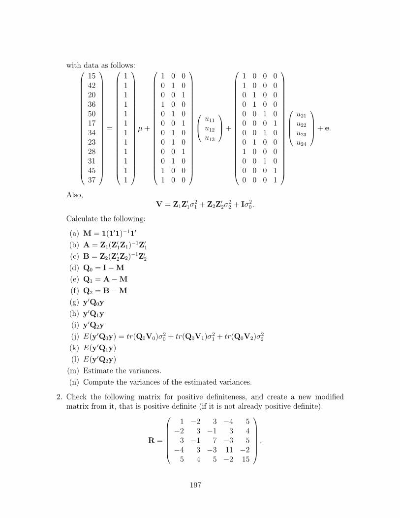
with data as follows:
154220365017342328314537
=
111111111111
µ+
1 0 00 1 00 0 11 0 00 1 00 0 10 1 00 1 00 0 10 1 01 0 01 0 0
u11
u12
u13
+
1 0 0 01 0 0 00 1 0 00 1 0 00 0 1 00 0 0 10 0 1 00 1 0 01 0 0 00 0 1 00 0 0 10 0 0 1
u21
u22
u23
u24
+ e.
Also,V = Z1Z
′1σ
21 + Z2Z
′2σ
22 + Iσ2
0.
Calculate the following:
(a) M = 1(1′1)−11′
(b) A = Z1(Z′1Z1)
−1Z′1(c) B = Z2(Z
′2Z2)
−1Z′2(d) Q0 = I−M
(e) Q1 = A−M
(f) Q2 = B−M
(g) y′Q0y
(h) y′Q1y
(i) y′Q2y
(j) E(y′Q0y) = tr(Q0V0)σ20 + tr(Q0V1)σ
21 + tr(Q0V2)σ
22
(k) E(y′Q1y)
(l) E(y′Q2y)
(m) Estimate the variances.
(n) Compute the variances of the estimated variances.
2. Check the following matrix for positive definiteness, and create a new modifiedmatrix from it, that is positive definite (if it is not already positive definite).
R =
1 −2 3 −4 5−2 3 −1 3 4
3 −1 7 −3 5−4 3 −3 11 −2
5 4 5 −2 15
.
197

Likelihood Methods
104 Likelihood Functions
The multivariate normal distribution likelihood function is
L(y) = (2π)−.5N | V |−.5 exp(−.5(y −Xb)′V−1(y −Xb)).
The log of the likelihood, say L1 is
L1 = −0.5[N ln(2π) + ln | V | +(y −Xb)′V−1(y −Xb)].
The term N ln(2π) is a constant that does not involve any of the unknown variances oreffects in the model, and therefore, it is commonly omitted during maximization compu-tations. Maximizing the log likelihood maximizes the original likelihood function.
Previously,| V |=| R | | Z′R−1Z + G−1 | | G |,
and therefore,ln | V |= ln | R | + ln | G | + ln | Z′R−1Z + G−1 | .
If R = Iσ20, then
ln | R | = ln | Iσ20 |
= ln(σ20)N | I |
= N lnσ20(1).
Similarly, if G =∑+ Iσ2
i , where i = 1 to s, then
ln | G | =s∑i=1
ln | Iσ2i |
=s∑i=1
qi lnσ2i .
Except, that in animal models one of the Gi is equal to Aσ2i . In that case,
ln | Aσ2i |= ln(σ2
i )qi | A |
which isln | Aσ2
i |= qi lnσ2i | A | = qi lnσ
2i + ln | A | .
Recall that
C =
(X′R−1X X′R−1ZZ′R−1X Z′R−1Z + G−1
),
198

and| C |=| Z′R−1Z + G−1 | | X′V−1X |
so thatln | C |= ln | Z′R−1Z + G−1 | + ln | X′V−1X | .
105 Maximum Likelihood Method
Hartley and Rao (1967) described the maximum likelihood approach for the estimationof variance components. Let L2 be equivalent to L1 except for the constant involving π.
L2 = −0.5[ln | V | +(y −Xb)′V−1(y −Xb)].
The derivatives of L2 with respect to b and to σ2i for i = 0, 1, . . . s are
∂L2
∂b= X′V−1Xb−X′V−1y
and
∂L2
∂σ2i
= −.5 tr[V−1(∂V/∂σ2i )]
+ .5(y −Xb)′V−1(∂V/∂σ2i )V
−1(y −Xb)
= −.5 tr[V−1Vi] + .5(y −Xb)′V−1ViV−1(y −Xb)
Equating the derivatives to zero gives
b = (X′V−1X)−X′V−1y,
andtr[V−1Vi] = (y −Xb)′V−1ViV
−1(y −Xb).
Recall thatPy = V−1(y −Xb),
where P is the projection matrix, and that Vi = ZiZ′i, then
tr[V−1ZiZ′i] = y′PViPy.
In usual mixed model theory, the solution vector for a random factor may be written as
ui = GiZ′iPy,
so that
y′PViPy = y′PZiGiG−2i GiZ
′iPy
= u′iG−2i ui
= u′iui/σ4i .
199

Also,
tr[V−1Vi] = tr[(R−1 −R−1Z(Z′R−1Z + G−1)−1Z′R−1)ZiZ′i].
Let
T = (Z′R−1Z + G−1)−1,
R = Iσ20,
and G =+∑
Iσ2i ,
thentr[V−1Vi] = tr(Z′iZi)σ
−20 − tr(Z′iZTZ′Zi)σ
−40 .
If T can be partitioned into submatrices for each random factor, then
Tσ−20 (Z′Z +
+∑Iαi) = I,
and
TZ′Zσ−20 = I−T(
+∑Iσ−2
i ),
TZ′Ziσ−20 = I−Tiiσ
−2i ,
which yields
tr(Z′iZTZ′Zi)σ−40 = tr(Z′iZi)σ
−20 − tr(I−Tiiσ
−2i )σ−2
i .
Finally,
tr[V−1Vi] = tr(I−Tiiσ−2i )σ−2
i
= trIσ−2i − trTiiσ
−4i
= qiσ−2i − trTiiσ
−4i .
Combining results givesσ2i = (u′iui + trTiiσ
20)/qi
for i = 1, 2, . . . , s, and for i = 0 gives
σ20 = (y′y − b′X′y − u′Z′y)/ N.
105.1 The EM Algorithm
EM stands for Expectation Maximization. The procedure alternates between calculatingconditional expected values and maximizing simplified likelihoods. The actual data y arecalled the incomplete data in the EM algorithm, and the complete data are considered to
200

be y and the unobservable random effects, ui. If the realized values of the unobservablerandom effects were known, then their variance would be the average of their squaredvalues, i.e.,
σ2i = u′iui/qi.
However, in real life the realized values of the random effects are unknown.
The steps of the EM algorithm are as follows:
Step 0. Decide on starting values for the variances and set m = 0.
Step 1.(E-step) Calculate the conditional expectation of the sufficient statistics, condi-tional on the incomplete data.
E(u′iui | y) = σ4(m)i y′P(m)ZiZ
′iP
(m)y
+tr(σ2(m)i I− σ4(m)
i Z′i(V(m))−1Zi)
= t(m)i
Step 2.(M-step) Maximize the likelihood of the complete data,
σ2(m+1)i = t
(m)i /qi, i = 0, 1, 2, . . . , s.
Step 3. If convergence is reached, set σ = σ(m+1), otherwise increase m by one andreturn to Step 1.
This is equivalent to constructing and solving the mixed model equations with a given setof variances, σ(m), and then
σ2(m+1)0 = (y′y − b′X′y − u′Z′y)/N,
and σ2(m+1)i = (u′iui + σ
2(m+1)0 trTii)/qi.
201

106 Restricted Maximum Likelihood Method
Restricted (or Residual) maximum likelihood (REML), was first suggested by Thompson(1962), and described formally by Patterson and Thompson (1971). The procedure re-quires that y has a multivariate normal distribution. The method is translation invariant.The maximum likelihood approach automatically keeps the estimator within the allowableparameter space(i.e. zero to plus infinity), and therefore, REML is a biased procedure.REML was proposed as an improvement to ML in order to account for the degrees offreedom lost in estimating fixed effects.
The likelihood function used in REML is that for a set of error contrasts (i.e. resid-uals) assumed to have a multivariate normal distribution. The multivariate normal dis-tribution likelihood function for the residual contrasts, K′y, where K′X = 0, and K′ hasrank equal to N − r(X), is
L(K′y) = (2π)−.5(N−r(X)) | K′VK |−.5 exp(−.5(K′y)′(K′VK)−1(K′y)).
The natural log of the likelihood function is
L3 = −.5(N − r(X)) ln(2π)− .5 ln | K′VK | −.5y′K(K′VK)−1K′y.
Notice that −.5(N − r(X)) ln(2π) is a constant that does not depend on the unknownvariance components or factors in the model, and therefore, can be ignored to give L4.Searle (1979) showed that
ln | K′VK | = ln | V | + ln | X′V−1X |
andy′K(K′VK)−1K′y = y′Py = (y −Xb)′V−1(y −Xb)
for any K′ such that K′X = 0. Hence, L4 can be written as
L4 = −.5 ln | V | −.5 ln | X′V−1X | −.5(y −Xb)′V−1(y −Xb).
REML can be calculated a number of different ways.
1. Derivative Free approach is a search technique to find the parameters that max-imize the log likelihood function. Two techniques will be described here.
2. First Derivatives and EM is where the first derivatives of the log likelihood aredetermined and set to zero in order to maximize the likelihood function. Solutionsneed to be obtained by iteration because the resulting equations are non linear.
3. Second Derivatives are generally more computationally demanding. Gradientmethods are used to find the parameters that make the first derivatives equal to zero.Newton-Raphson (involves the observed information matrix) and Fishers Methodof Scoring (involves the expected information matrix) have been used. Lately, the”average information” algorithm (averages the observed and expected informationmatrices) has been used to reduce the computational time.
202

106.1 Example Problem
All of the approaches attempt to maximize the log likelihood function of the error con-trasts. To illustrate the methods, consider a single trait model with three factors (F,A,B),of which A and B are random factors. There were a total of 90 observations, and thetotal sum of squares was 356,000. The least squares equations for this small example areshown below.
50 0 5 15 30 5 10 20 150 40 5 15 20 5 10 20 55 5 10 0 0 2 3 4 1
15 15 0 30 0 5 7 11 730 20 0 0 50 3 10 25 125 5 2 5 3 10 0 0 0
10 10 3 7 10 0 20 0 020 20 4 11 25 0 0 40 015 5 1 7 12 0 0 0 20
F1
F2
A1
A2
A3
B1
B2
B3
B4
=
32002380580
18603140700
132024001160
.
106.1.1 Derivative Free REML
Imagine an s dimensional array containing the values of the likelihood function for everypossible set of values of the ratios of the components to the residual variance. Thetechnique is to search this array and find the set of ratios for which the likelihood functionis maximized. There is more than one way to conduct the search. Care must be taken tofind the ’global’ maximum rather than one of possibly many ’local’ maxima. At the sametime the number of likelihood evaluations to be computed must also be minimized.
Various alternative forms of L4 can be derived. Note that
ln | V |= ln | R | + ln | G | + ln | G−1 + Z′R−1Z |
and thatln | X′V−1X |= ln | C | − ln | Z′R−1Z + G−1 |
and that combining these results gives
L4 = − .5 ln | R | −.5 ln | G | −.5 ln | C | −.5y′Py.
Now note that
ln | R | = ln | Iσ20 |
= N lnσ20,
ln | G | =s∑i=1
qi lnσ2i ,
203

and ln | C | = ln | X′R−1X | + ln | Z′SZ + G−1 |where ln | X′R−1X | = ln | X′Xσ−2
0 |= ln(σ−2
0 )r(X) | X′X |= ln | X′X | −r(X) lnσ2
0,
and Z′SZ + G−1 = σ−20 Z′MZ + G−1
= σ−20 (Z′MZ + G−1σ2
0).
Thenln | C |= ln | X′X | −r(X) lnσ2
0 − q lnσ20 + ln | Z′MZ + G−1σ2
0 |,
and finally, the log-likelihood function becomes
L4 = −.5(N − r(X)− q) lnσ20 − .5
s∑i=1
qi lnσ2i
−.5 ln | C? | −.5y′Py,
where
C? =
(X′X X′ZZ′X Z′Z + G−1σ2
0
).
Note that
qi lnσ2i = qi lnσ
20/αi
= qi(lnσ20 − lnαi)
so that
L4 = −.5[(N − r(X)) lnσ20 −
s∑i=1
qi lnαi + ln | C? | +y′Py].
The quantity y′Py is y′(y − Xb − Zu)/σ20. The computations are achieved by
constructing the following matrix, X′X X′Z X′yZ′X Z′Z + G−1σ2
0 Z′yy′X y′Z y′y
=
(C? W′yy′W y′y
),
then by Gaussian elimination of one row at a time, the sum of the log of the non-zeropivots (using the same ordering for each evaluation of the likelihood) gives log | C? | andy′(y − Xb − Zu). Gaussian elimination, using sparse matrix techniques, requires lesscomputing time than inverting the coefficient matrix of the mixed model equations. Theordering of factors within the equations could be critical to the computational process andsome experimentation may be necessary to determine the best ordering. The likelihoodfunction can be evaluated without the calculation of solutions to the mixed model equa-tions, without inverting the coefficient matrix of the mixed model equations, and without
204

computing any of the σ2i . The formulations for more general models and multiple trait
models are more complex, but follow the same ideas.
Searching the array of likelihood values for various values of αi can be done in severaldifferent ways. One method is to fix the values of all but one of the s αi, and then evaluateL2 for four or more different values of the αi that were not fixed. Then one can use aquadratic regression analysis to determine the value of that one ratio which maximizesL2 given that the other ratios are fixed. This is repeated for each of the s ratios, andthe process is repeated until a maximum likelihood is obtained. The calculations aredemonstrated in the example that follows.
Begin by fixing the value of αB = 10 and letting the value of αA take on the values of(5, 10, 20, 30, 40). Using L4 to evaluate the likelihood, then the results were as follows:
αA L4
5 -251.444210 -251.150420 -250.982230 -250.927440 -250.9019
For example, the likelihood value for αA = 40, would be
L4 = −1
2[(N − r(X)) lnσ2
0 − qA lnαA − qB lnαB + ln | C? | +y′(y −Xb− Zu)/σ20]
where
ln | C? | = 32.052454,
y′Py = 8483.176/σ20 = 88,
qA lnαA = 11.0666385,
qB lnαB = 9.2103404,
σ20 = 96.399728,
lnσ20 = 4.5685034,
(N − r(X)) = 88,
then
L4 = −0.5[88(4.5685)− 11.0666− 9.2103 + 32.0525 + (8483.176/96.3997)]
= −250.9019.
205

To find the value of αA that maximizes L4 for αB = 10, let
Q =
1 5 251 10 1001 20 4001 30 9001 40 1600
and Y =
−251.4442−251.1504−250.9822−250.9274−250.9019
then
β = (Q′Q)−1Q′Y =
−251.6016.0448877−.000698
.From this a prediction equation for L4 can be written as
L4 = − 251.6016 + .04489αA − .000698α2A.
This equation can be differentiated with respect to αA and then equated to zero to findthe value of the ratio that maximizes the prediction equation. This gives
αA = .04489/(2(.000698)) = 32.1546.
Now keep αA = 32.1546 and try a number of values of αB from 2 to 10, which givethe following results.
αB L4
2 -250.27223 -250.19544 -250.23795 -250.32956 -250.44197 -250.56248 -250.68439 -250.8042
10 -250.9204
Applying the quadratic regression to these points gives
αB = 1.2625.
The next step would be to fix αB = 1.2625 and to try new values for αA, such as25 to 40 by units of 1. The range of values becomes finer and finer. To insure that onehas found the global maximum, the entire process could be started with vastly differentstarting values for the ratios, such as αB = 50 and let values for αA be 40, 50, 60, and
206

70. The more components there are to estimate, the more evaluations of the likelihoodthat are going to be needed, and the more probable that convergence might be to a localmaximum rather than to the global maximum.
Please refer to the literature for specification of the log likelihood function for par-ticular models and situations.
106.1.2 The Simplex Method
The Simplex Method (Nelder and Mead, 1965) is a procedure for finding the minimumof a function (i.e. the minimum of −2L4 or the maximum of L4) with respect to theunknown variances and covariances. The best way to describe the method is using theexample data from the previous sections. Begin by constructing a set of ’points’ for whichL4 is to be evaluated. A ’point’ is a vector of values for the unknowns ( αA, αB), forexample,
θ1 =(
12.1 3.8),
then form two more points by changing one unknown at a time. Let the three points beas shown in the following table.
No. αA αB1 12.1 3.82 13.1 3.83 12.1 4.3
Now calculate L4 for each point and arrange from largest to lowest value.
No. αA αB L4
2 13.1 3.8 -250.30471 12.1 3.8 -250.31973 12.1 4.3 -250.3662
The idea now is to find another point to replace the last one(lowest L4). This is doneby a process called reflection. Compute the mean of all points excluding the one with thelowest L4.
θm =(
12.6 3.8),
then the reflection step isθ4 = θm + r ∗ (θm − θlast),
where r is recommended by Nelder and Mead (1965) to be 1, giving
θ4 =(
13.1 3.3).
207

The corresponding L4 for this point was -250.2722. Compared to those in the table it hasthe largest value, and therefore, is a better point than the other three.
No. αA αB L4
4 13.1 3.3 -250.27222 13.1 3.8 -250.30471 12.1 3.8 -250.3197
Given this success, the Simplex method calls for an expansion step, i.e. to make abigger change. Thus,
θ5 = θm + E ∗ (θ4 − θm),
where E is suggested to be equal to 2. Hence
θ5 =(
13.6 2.8).
Then L4 = −250.2546, and the expanded point is better yet. Now drop θ1 from the tableand put θ5 at the top.
No. αA αB L4
5 13.6 2.8 -250.25464 13.1 3.3 -250.27222 13.1 3.8 -250.3047
This completes one iteration. Begin the next iteration by computing the mean of allpoints excluding the point with the lowest L4.
θm =(
13.35 3.05).
Another reflection step gives
θ6 = θm + r ∗ (θm − θlast),=
(13.6 2.3
).
However, this gives L4 = −250.2761, which is between θ2 and θ4, and can push out θ2
from the table.
No. αA αB L4
5 13.6 2.8 -250.25464 13.1 3.3 -250.27226 13.6 2.3 -250.2761
208

Instead of an expansion step, a contraction step is needed because θ6 did not give agreater L4 than the first two. Thus,
θ7 = θm + c ∗ (θ6 − θm),
where c = 0.5 is recommended. Hence,
θ7 =(
13.475 3.05).
Then L4 = −250.2586 is better than that given by θ4, but not by θ5, thus the new tablebecomes as follows:
No. αA αB L4
5 13.6 2.8 -250.25467 13.475 3.05 -250.25864 13.1 3.3 -250.2722
The following steps were taken in the next iteration.
1. The mean of the top two L4 is
θm =(
13.5375 2.925).
2. A reflection step gives
θ8 = θm + r ∗ (θm − θlast),=
(13.975 2.55
),
which gave L4 = −250.2563, which is better than θ7.
3. Add θ8 to the table and drop θ4.
No. αA αB L4
5 13.6 2.8 -250.25468 13.975 2.55 -250.25637 13.475 3.05 -250.2586
4. Because L4 for θ8 was not larger than L4 for θ5 or smaller than L4 for θ7, then noexpansion or contraction step is necessary. Begin the next iteration.
The Simplex method continues in this manner until all point entries in the table areequal. The constants recommended by Nelder and Mead (1965) for reflection, expansion,and contraction could be adjusted for a particular data set. This method may converge toa local maximum, and so different starting values are needed to see if it converges to thesame point. The Simplex method does not work well with a large number of parametersto be estimated.
209
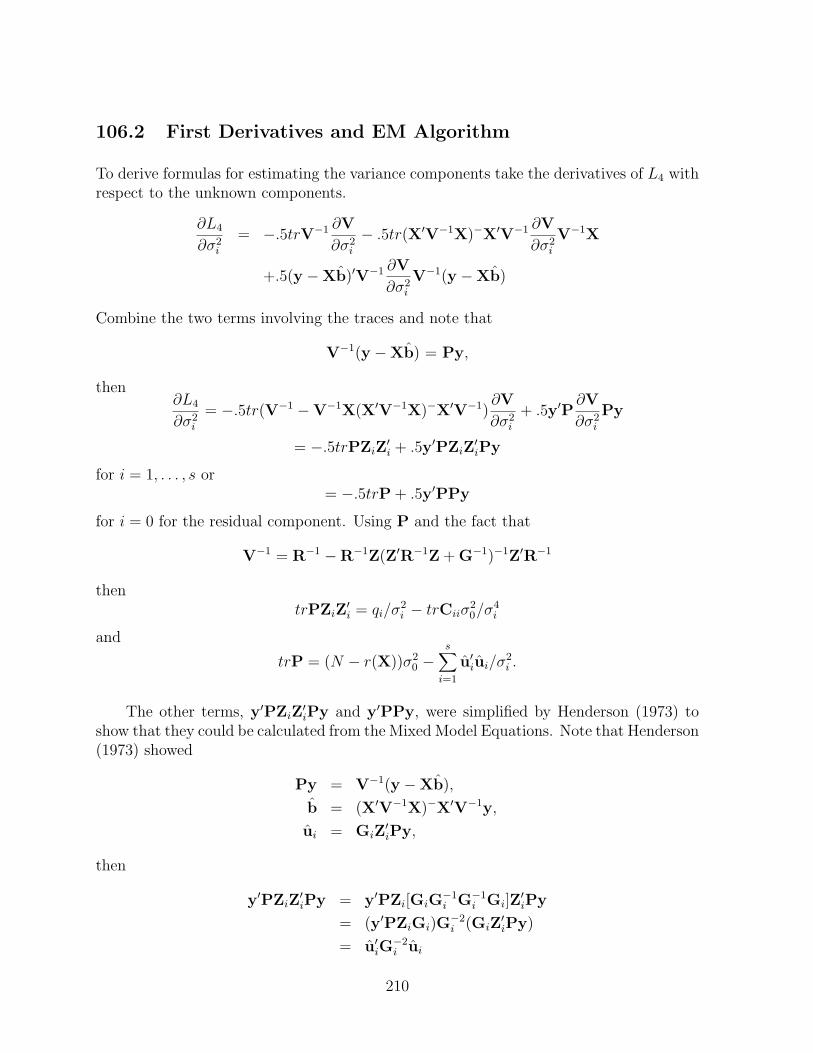
106.2 First Derivatives and EM Algorithm
To derive formulas for estimating the variance components take the derivatives of L4 withrespect to the unknown components.
∂L4
∂σ2i
= −.5trV−1 ∂V
∂σ2i
− .5tr(X′V−1X)−X′V−1 ∂V
∂σ2i
V−1X
+.5(y −Xb)′V−1 ∂V
∂σ2i
V−1(y −Xb)
Combine the two terms involving the traces and note that
V−1(y −Xb) = Py,
then∂L4
∂σ2i
= −.5tr(V−1 −V−1X(X′V−1X)−X′V−1)∂V
∂σ2i
+ .5y′P∂V
∂σ2i
Py
= −.5trPZiZ′i + .5y′PZiZ
′iPy
for i = 1, . . . , s or= −.5trP + .5y′PPy
for i = 0 for the residual component. Using P and the fact that
V−1 = R−1 −R−1Z(Z′R−1Z + G−1)−1Z′R−1
thentrPZiZ
′i = qi/σ
2i − trCiiσ
20/σ
4i
and
trP = (N − r(X))σ20 −
s∑i=1
u′iui/σ2i .
The other terms, y′PZiZ′iPy and y′PPy, were simplified by Henderson (1973) to
show that they could be calculated from the Mixed Model Equations. Note that Henderson(1973) showed
Py = V−1(y −Xb),
b = (X′V−1X)−X′V−1y,
ui = GiZ′iPy,
then
y′PZiZ′iPy = y′PZi[GiG
−1i G−1
i Gi]Z′iPy
= (y′PZiGi)G−2i (GiZ
′iPy)
= u′iG−2i ui
210

which when Gi = Iσ2i gives
u′iui/σ4i .
Similarly for the residual component, Henderson showed that
y′PPy = [y′y − b′X′y −s∑i=1
(u′iZ′iy + u′iuiαi)]/σ
20,
where αi = σ20/σ
2i .
Equate the derivatives to zero incorporating the above simplifications and obtain
σ2i = (u′iui + trCiiσ
20)/qi,
σ20 = y′Py/(N − r(X)).
As with ML, solutions using the EM algorithm must be computed iteratively. Convergenceis usually very slow, if it occurs, and the process may also diverge.
Notice the differences between REML and ML. The denominator for σ20 is N − r(X)
rather than N , and in σ2i is trCii rather than trTii. The quadratic forms, however, are
identical in REML and ML. Accounting for the degrees of freedom to estimate b hasresulted in the REML algorithm.
A major computing problem with the EM algorithm is the calculation of trCii, whichis the corresponding inverse elements of the mixed model equations for the ith randomfactor. With most applications in animal breeding, the order of the mixed model equationsare too large to be inverted, and solutions to the equations are obtained by Gauss-Seideliterations. However, there have been several attempts to approximate trCii, but thesehave not been totally suitable.
To demonstrate the EM algorithm let αA = 10 and αB = 5 be the starting values ofthe ratios for factors A and B, respectively. There were N = 90 total observations, andr(X) = 2. The solution vector is
F1
F2
A1
A2
A3
B1
B2
B3
B4
=
64.631359.4225−2.1363.4955
1.63685.10642.6402−2.6433−5.1034
.
Theny′(Xb + Zu) = 347, 871.2661
211

and from the inverse of the coefficient matrix,
trCAA = .16493, and trCBB = .3309886
which give rise to the following estimates,
σ20 = (356, 000− 347, 871.2661)/88
= 92.371976,
σ2A = (7.4925463 + .16493(92.371976))/3
= 7.575855,
σ2B = (66.0771576 + .3309886(92.371976))/4
= 24.16280774.
New ratios are formed as
αA = 92.371976/7.575855 = 12.192944,
andαB = 92.371976/24.16280774 = 3.822899
and these are used to form the mixed model equations again, new solutions and tracesare calculated, and so on, until the estimated ratios and the prior values of the ratios areequal. The estimates converge to
σ20 = 91.8639,
σ2A = 2.5692,
σ2B = 30.5190.
orαA = 35.7558, and αB = 3.0101.
106.3 Second Derivatives, Average Information
Second derivatives of the log likelihood lead to the expectations of the quadratic forms.One technique, MIVQUE (Minimum Variance Quadratic Unbiased Estimation) equatesthe quadratic forms to their expectations. The estimates are unbiased and if all variancesremain positive, then convergence will be to the REML estimates. However, due to ashortage of data or an inappropriate model, the estimates derived in this manner can benegative. Computing the expectations of the quadratic forms requires the inverse of themixed model equations coefficient matrix, and then products and crossproducts of variousparts of the inverse.
212

A gradient method using first and second derivatives can be used (Hofer, 1998). Thegradient, d ( the vector of first derivatives of the log likelihood), is used to determine thedirection towards the parameters that give the maximum of the log likelihood, such that
θ(t+1) = θ(t) + M(t)d(t),
where d(t) are the first derivatives evaluated at θ = θ(t), and M(t) in the Newton-Raphson(NR) algorithm is the observed information matrix, and in the Fisher Method ofScoring(FS) it is the expected information matrix.
The first derivatives are as follows (from earlier in these notes):
∂L4
∂σ2i
= −.5trPZiZ′i + .5y′PZiZ
′iPy = 0
for i = 1, . . . , s or∂L4
∂σ20
= −.5trP + .5y′PPy = 0
for the residual component. Then from earlier results,
trPZiZ′i = qi/σ
2i − trCiiσ
20/σ
4i ,
y′PZiZ′iPy = u′iui/σ
4i
which combined give
0.5(u′iui/σ4i − qi/σ2
i + trCiiσ20/σ
4i ) = 0,
for i = 1, . . . , s, and
trP = (N − r(X))σ20 −
s∑i=1
u′iui/σ2i
y′PPy = [y′y − b′X′y −s∑i=1
(u′iZ′iy + u′iuiαi)]/σ
20
which combined give
0.5([y′y − b′X′y −s∑i=1
(u′iZ′iy + u′iuiαi)]/σ
20 − (N − r(X))σ2
0 +s∑i=1
u′iui/σ2i ) = 0,
which simplifies to
0.5([y′y − b′X′y −s∑i=1
u′iZ′iy]/σ2
0 − (N − r(X))σ20) = 0.
213

The second derivatives give a matrix of quantities. The elements of the observedinformation matrix (Gilmour et al. 1995) are
− ∂2L4
∂σ2i ∂σ
20
= 0.5y′PZiZ′iPy/σ4
0,
− ∂2L4
∂σ2i ∂σ
2j
= 0.5tr(PZiZ′j)− 0.5tr(PZiZ
′iPZjZ
′j)
+y′PZiZ′iPZjZ
′jPy/σ2
0 − 0.5y′PZiZ′jPy/σ2
0,
and
− ∂2L4
∂σ20∂σ
20
= y′Py/σ60 − 0.5(N − r(X))/σ4
0.
The elements of the expected information matrix (Gilmour et al. 1995) are
E[− ∂2L4
∂σ2i ∂σ
20
] = 0.5tr(PZiZ′i)/σ
20,
E[− ∂2L4
∂σ2i ∂σ
2j
] = 0.5tr(PZiZ′iPZjZ
′j),
and
E[− ∂2L4
∂σ20∂σ
20
] = 0.5(N − r(X))/σ40.
As the name Average Information implies, average the observed and expected informationmatrices to give the following matrix of elements.
I[σ2i , σ
20] = 0.5y′PZiZ
′iPy/σ4
0,
I[σ2i , σ
2j ] = y′PZiZ
′iPZjZ
′jPy/σ2
0,
and
I[σ20, σ
20] = 0.5y′Py/σ6
0.
The first derivatives form the vector, d(t), and
M(t) = I[σ, σ]−1.
The rest of this method is computational detail to simplify the requirements for inverseelements and solutions to MME. The calculations can not be illustrated very easily forthe example data because the y-vector is not available.
106.4 Animal Models
The model commonly applied to estimation of variance components in livestock geneticssince 1989 has been an animal model. The animal model assumes a large, random mating
214

population, an infinite number of loci each with a small and equal effect on the trait, onlyadditive genetic effects, and all relationships among animals are known and tracible to anunselected base population (somewhere in the past). Animals may have more than onerecord each. The equation of the model is
y = Xb + Za + Zp + e,
where a is the vector of animal additive genetic effects (one per animal), and p is a vectorof permanent environmental (p.e.) effects associated with each animal.
E(y) = Xb,
V ar
ape
=
Aσ2a 0 0
0 Iσ2p 0
0 0 Iσ2e
.The matrix A is called the numerator relationship matrix. Wright defined relationshipsamong animals as correlations, but A is essentially relationships defined as covariances(the numerators of the correlation coefficients). Also, these only represent the additivegenetic relationships between animals.
The MME for this model are X′X X′Z X′ZZ′X Z′Z + A−1ka Z′ZZ′X Z′Z Z′Z + Ikp
b
ap
=
X′yZ′yZ′y
.Note that ka is the ratio of residual to additive genetic variances, and kp is the ratioof residual to permanent environmental variances. Also, in MME the inverse of A isrequired.
The EM-REML procedure gives
σ2e = (y′y − b′X′y − a′Z′y − p′Z′y)/(N − r(X)),
σ2a = (a′A−1a + trA−1Caaσ
2e)/n,
σ2p = (p′p + trCppσ
2e)/n,
where n is the total number of animals, N is the total number of records, and Caa arethe inverse elements of the MME for the animal additive genetic effects, and Cpp arethe inverse elements of the MME for the animal permanent environmental effects. Anexample of this model will be given in later notes.
106.4.1 Quadratic Forms in an Animal Model
A necessary quadratic form in an animal model is a′A−1a, and this can be computed veryeasily. Note that the inverse of A may be written as
A−1 = T−1D−2T′−1,
215

where T−1 is an upper triangular matrix, and diagonal matrix D−2 has elements equalto 1, 2, or 4/3 in noninbred situations, and values greater than 2 in inbred situations. InHenderson (1975), this inverse was shown to be composed of just three numbers, i.e. 0,1’s on the diagonals, and -.5 corresponding to the parents of an animal. For example,
T′−1
=
1 0 0 00 1 0 0
−.5 −.5 1 0−.5 0 −.5 1
.
Then
T′−1
a = m
= (ai − 0.5(as + ad)),
for the ith animal, and as and ad are the sire and dam estimated breeding values, respec-tively. Consequently,
a′A−1a = a′T−1B−2T′−1
a
= m′B−2m
=q∑i=1
m2i bii,
where bii are the diagonal elements of B−2, and q is the number of animals.
107 EXERCISES
Below are pedigrees and data on 20 animals.
216

Animal Sire Dam Group Record1 - -2 - -3 - -4 - -5 1 2 1 286 1 2 1 407 3 4 1 308 1 2 1 359 1 4 2 1710 3 2 2 4111 1 4 2 2312 3 2 2 3813 1 2 2 3714 3 4 2 2715 5 7 3 2416 6 14 3 3117 8 7 3 4218 1 10 3 4719 3 13 3 2620 5 9 3 33
1. Construct A−1 and set up the MME.
2. Apply EM-REML to the model,
yij = µ+ gi + aj + eij,
where group, animal additive genetic, and residual effects are random. Let
σ2e/σ
2a = 1.5, σ2
e/σ2g = 5.0,
to start the iterations. Do five iterations of EM-REML.
3. Apply EM-REML again to the model with
σ2e/σ
2a = 3.0, σ2
e/σ2g = 2.5,
and do five iterations of REML from these starting values.
4. Do the results of the previous two question tend to give similar answers? Commenton the results.
5. Use the Derivative Free method and compute the log likelihoods for various sets ofparameters.
217

Bayesian Methods
Every variable in a linear model is a random variable derived from a distributionfunction. A fixed factor becomes a random variable with possibly a uniform distributiongoing from a lower limit to an upper limit. A component of variance is a random variablehaving a Gamma or Chi-square distribution with df degrees of freedom. In addition, theresearcher may have information from previous experiments that strongly indicate thevalue that a variance component may have, and the Bayes approach allows the aprioriinformation to be included in the analysis.
The Bayesian process is to
1. Specify distributions for each random variable of the model.
2. Combine the distributions into the joint posterior distribution.
3. Find the conditional marginal distributions from the joint posterior distribution.
4. Employ Markov Chain Monte Carlo (MCMC) methods to maximize the joint poste-rior distribution. Gibbs Sampling is a tool in MCMC methods for deriving estimatesof parameters from the joint posterior distribution.
By determining conditional marginal distributions for each random variable of themodel, then generating random samples from these distributions eventually converge torandom samples from the joint posterior distribution. Computationally, any program thatcalculates solutions to Henderson’s mixed model equations can be modified to implementGibbs Sampling.
108 The Joint Posterior Distribution
Begin with a simple single trait animal model. That is,
y = Xb + Za + e.
Let θ be the vector of random variables and y is the data vector, then
p(θ,y) = p(θ) p(y | θ)= p(y) p(θ | y)
Re-arranging gives
p(θ | y) =p(θ)p(y | θ)
p(y)
218

= (prior for θ)p(y | θ)p(y)
= posterior probability function of θ
In terms of the simple animal model, θ includes b, a, σ2a, and σ2
e .
108.1 Conditional Distribution of Data Vector
The conditional distribution of y given θ is
y | b, a, σ2a, σ
2e ∼ N(Xb + Za, Iσ2
e),
and
p(y | b, a, σ2a, σ
2e) ∝ (σ2
e)(−N/2) exp
[−(y −Xb− Za)′(y −Xb− Za)/2σ2
e
].
108.2 Prior Distributions of Random Variables
108.2.1 Fixed Effects Vector
There is little prior knowledge about the values in b might have. This is represented byassuming
p(b) ∝ constant.
108.2.2 Random Effects and Variances
For a, the vector of additive genetic values, quantitative genetics theory suggests thatthey follow a normal distribution, i.e.
a | A, σ2a ∼ N(0,Aσ2
a)
andp(a) ∝ (σ2
a)(−q/2) exp
[−a′A−1a/2σ2
a
],
where q is the length of a.
A natural estimator of σ2a is a′A−1a/q, call it S2
a, where
S2a ∼ χ2
qσ2a/q.
Multiply both sides by q and divide by χ2q to give
σ2a ∼ qS2
a/χ2q
219

which is a scaled, inverted Chi-square distribution, written as
p(σ2a | va, S2
a) ∝ (σ2a)−( va
2+1) exp
(−va
2
S2a
σ2a
),
where va and S2a are hyperparameters with S2
a being a prior guess about the value of σ2a
and va being the degrees of belief in that prior value. Usually q is much larger than vaand therefore, the data provide nearly all of the information about σ2
a.
108.2.3 Residual Effects
Similarly, for the residual variance,
p(σ2e | ve, S2
e ) ∝ (σ2e)−( ve
2+1) exp
(−ve
2
S2e
σ2e
).
108.2.4 Combining Prior Distributions
The joint posterior distribution is
p(b, a, σ2a, σ
2e | y) ∝ p(b)p(a | σ2
a)p(σ2a)p(σ
2e)p(y | b, a, σ2
a, σ2e)
which can be written as
∝ (σ2e)−(N+ve
2+1) exp
[− 1
2σ2e
((y −Xb− Za)′(y −Xb− Za) + veS2e )
]
(σ2a)−( q+va
2+1) exp
[− 1
2σ2a
(a′A−1a + vaS2a)
].
109 Fully Conditional Posterior Distributions
In order to implement Gibbs sampling, all of the fully conditional posterior distributions(one for each component of θ ) need to be derived from the joint posterior distribution.The conditional posterior distribution is derived from the joint posterior distribution bypicking out the parts that involve the unknown parameter in question.
220

109.1 Fixed and Random Effects of the Model
Let
W = (X Z),
β′ = (b′ a′),
Σ =
(0 00 A−1k
),
C = Henderson′s Mixed Model Equations
= W′W + Σ
Cβ = W′y
A new notation is introduced, let
β′ = (βi β′−i),
where βi is a scalar representing just one element of the vector β, and β−i is a vectorrepresenting all of the other elements except βi. Similarly, C and W can be partitionedin the same manner as
W′ = (Wi W−i)′
C =
(Ci,i Ci,−i
C−i,i C−i,−i
).
In general terms, the conditional posterior distribution of β is a normal distribution,
βi | β−i, σ2a, σ
2e ,y ∼ N(βi, C
−1i,i σ
2e)
whereCi,iβi = (W′
iy −Ci,−iβ−i).
Thenbi | b−i, a, σ2
a, σ2e ,y ∼ N(bi, C
−1i,i σ
2e),
forCi,i = x′ixi.
Also,ai | b, a−i, σ2
a, σ2e ,y ∼ N(ai, C
−1i,i σ
2e),
where Ci,i = (z′izi + Ai,ik), for k = σ2e/σ
2a.
221

109.2 Variances
The conditional posterior distributions for the variances are inverted Chi-square distribu-tions,
σ2a | b, a, σ2
e ,y ∼ vaS2aχ−2va
for va = q + va, and S2a = (a′A−1a + vaS
2a)/va, and
σ2e | b, a, σ2
a,y ∼ veS2eχ−2ve
for ve = N + ve, and S2e = (e′e + veS
2e )/ve, and e = y −Xb− Za.
110 Computational Scheme
Gibbs sampling is much like Gauss-Seidel iteration. When a new solution is calculatedin the Mixed Model Equations for a level of a fixed or random factor, a random amountis added to the solution based upon its conditional posterior distribution variance beforeproceeding to the next level of that factor or the next factor. After all equations havebeen processed, new values of the variances are calculated and a new variance ratio isdetermined prior to beginning the next round. The following MME for five animals willbe used to illustrate the Gibbs sampling scheme:
5 1 1 1 1 11 29 7 −7 −14 01 7 30 −14 8 −161 −7 −14 36 −14 01 −14 8 −14 37 −161 0 −16 0 −16 33
µa1
a2
a3
a4
a5
=
238.238.548.964.350.536.0
,
where k = σ2e/σ
2a = 14, and
A−1 =1
14
28 7 −7 −14 07 29 −14 8 −16−7 −14 35 −14 0−14 8 −14 36 −16
0 −16 0 −16 32
.
The starting values for β =(
0 0 0 0 0 0), and for va = ve = 10, and S2
e = 9313
and S2a = 62
3, so that k = 14. Let RND represent a random normal deviate from a random
normal deviate generator, and let CHI(idf) represent a random Chi-square variate from arandom Chi-Square variate generator with idf degrees of freedom. Every time that RNDand CHI(idf) appear, a different random number is generated for that expression.
To begin, let σ2e = S2
e and σ2a = S2
a. Below are descriptions of calculations in the firsttwo rounds.
222

110.1 Round 1
110.1.1 Fixed and Random Effects of Model
• Overall mean
µ = (238.2− a1 − a2 − a3 − a4 − a5)/5
= 47.64
µ = µ+RND ∗ (σ2e/5).5
= 47.64 + (−1.21) ∗ (4.32)
= 42.41
• Animal 1
a1 = (38.5− µ− 7a2 + 7a3 + 14a4)/29
= −.1349
a1 = a1 +RND ∗ (σ2e/29).5
= −.1349 + (1.138)(1.794)
= 1.9067
• Animal 2
a2 = (48.9− µ− 7a1 + 14a3 − 8a4 + 16a5)/30
= −6.8591/30 = −.2286
a2 = a2 +RND ∗ (σ2e/30).5
= −.2286 + (.0047)(1.7638)
= −.2203
• Animal 3
a3 = (64.3− µ+ 7a1 + 14a2 + 14a4)/36
= .8931
a3 = a3 +RND ∗ (σ2e/36).5
= .8931 + (−1.1061)(1.6102)
= −.8879
223

• Animal 4
a4 = (50.5− µ+ 14a1 − 8a2 + 14a3 + 16a5)/37
= .6518
a4 = a4 +RND ∗ (σ2e/37).5
= .6518 + (−1.2293)(1.5882)
= −1.3006
• Animal 5
a5 = (36.0− µ+ 16a2 + 16a4)/33
= −.9316
a5 = a5 +RND ∗ (σ2e/33).5
= −.9316 + (−.6472)(1.6817)
= −2.0200
110.1.2 Residual Variance
Calculate the residuals and their sum of squares in order to obtain a new residualvariance.
e1 = 38.5− 42.41− 1.9067 = −5.8167
e2 = 48.9− 42.41 + .2203 = 6.7103
e3 = 64.3− 42.41 + .8879 = 22.7779
e4 = 50.5− 42.41 + 1.3006 = 9.3906
e5 = 36.0− 42.41 + 2.0200 = −4.3900
e′e = 705.1503
A new sample value of the residual variance is
σ2e = (e′e + veS
2e )/CHI(15)
= (705.1503 + (10)(93.3333))/17.1321
= 95.6382.
110.1.3 Additive Genetic Variance
The additive genetic variance requires calculation of a′A−1a using the a-values ob-tained above, which gives
a′A−1a = 19.85586.
224

Then
σ2a = (a′A−1a + vaS
2a)/CHI(15)
= (19.85586 + (10)(6.66667))/10.7341
= 8.0605.
A new sample value of the variance ratio becomes
k = 95.6382/8.0605 = 11.8650.
110.2 Round 2
Round 2 begins by re-forming the MME using the new variance ratio. The equationschange to
5 1 1 1 1 11 24.73 5.93 −5.93 −11.86 01 5.93 25.58 −11.86 6.78 −13.561 −5.93 −11.86 30.66 −11.86 01 −11.86 6.78 −11.86 31.51 −13.561 0 −13.56 0 −13.56 28.12
µa1
a2
a3
a4
a5
=
238.238.548.964.350.536.0
.
110.2.1 Fixed and Random Effects of Model
The process is repeated using the last values of µ and a and σ2e .
µ = (238.2− a1 − a2 − a3 − a4 − a5)/5
= 48.14
µ = µ+RND ∗ (σ2e/5).5
= 48.14 + (.7465) ∗ (4.3735)
= 51.41
a1 = (38.5− µ− 5.93a2 + 5.93a3 + 11.864)/24.73
= −1.3059
a1 = a1 +RND ∗ (σ2e/24.73).5
= −1.3059 + (−.0478)(1.9665)
= −1.3999
a2 = (48.9− µ− 5.93a1 + 11.86a3 − 6.78a4 + 13.56a5)/25.58
225

= −.9113
a2 = a2 +RND ∗ (σ2e/25.58).5
= −.9113 + (.8386)(1.9336)
= .7102
a3 = −2.41355/30.66
= −.0787
a3 = a3 +RND ∗ (σ2e/30.66).5
= −.0787 + (−1.8414)(1.7662)
= −3.3309
a4 = −89.2236/31.51 = −2.8316
a4 = −2.8316 + (−1.2549)(1.7422)
= −5.0179
a5 = −73.8224/28.12 = −2.6253
a5 = −2.6253 + (.8184)(1.8442)
= −1.1160
110.2.2 Residual Variance
The residuals and their sum of squares are
e1 = 38.5− 51.41 + 1.3999 = −11.5101
e2 = 48.9− 51.41− .7102 = −3.2202
e3 = 64.3− 51.41 + 3.3309 = 16.2209
e4 = 50.5− 51.41 + 5.0179 = 4.1079
e5 = 36.0− 51.41 + 1.1160 = −14.2940
e′e = 627.1630
The new sample value of the residual variance is
σ2e = (e′e + veS
2e )/CHI(15)
= (627.1630 + (10)(93.3333))/20.4957
= 76.1377.
226

110.2.3 Additive Genetic Variance
The new sample value of the additive genetic variance is
σ2a = (a′A−1a + vaS
2a)/CHI(15)
= (36.8306 + (10)(6.66667))/16.6012
= 6.2343.
The new variance ratio becomes
k = 76.1377/6.2343 = 12.2127.
Continue taking samples for thousands of rounds.
110.3 Burn-In Periods
The samples do not immediately represent samples from the joint posterior distribution.Generally, this takes anywhere from 100 to 10,000 samples depending on the model andamount of data. This period is known as the burn-in period. Samples from the burn-inperiod are discarded. The length of the burn-in period (i.e. number of samples) is usuallyjudged by visually inspecting a plot of sample values across rounds.
A less subjective approach to determine convergence to the joint posterior distributionis to run two chains at the same time, both beginning with the same random number seed.However, the starting values (in variances) for each chain are usually greatly different,e.g. one set is greatly above the expected outcome and the other set is greatly belowthe expected outcome. When the two chains essentially become one chain, i.e. thesquared difference between variance estimates is less than a specified value (like 10−5),then convergence to the joint posterior distribution has occurred. All previous samplesare considered to be part of the burn-in period and are discarded.
110.4 Post Burn-In Analysis
After burn-in, each round of Gibbs sampling is dependent on the results of the previousround. Depending on the total number of observations and parameters, one round maybe positively correlated with the next twenty to three hundred rounds. The user candetermine the effective number of samples by calculating lag correlations, i.e. the correla-tion of estimates between rounds, between every other round, between every third round,etc. Determine the number of rounds between two samples such that the correlation iszero. Divide the total number of samples (after burn-in) by the interval that gives a zerocorrelation, and that gives the effective number of samples. Suppose a total of 12,000
227
samples (after removing the burn-in rounds) and an interval of 240 rounds gives a zerocorrelation between samples, then the effective number of samples is 12,000 divided by 240or 50 samples. There is no minimum number of independent samples that are required,just the need to know how many there actually were.
An overall estimate of a parameter can be obtained by averaging all of the 12,000samples (after the burn-in). However, to derive a confidence interval or to plot the dis-tribution of the samples or to calculate the standard deviation of the sample values, thevariance of the independent samples should be used.
The final estimates are therefore, an average of the sample estimates. Some researchhas shown that the mode of the estimates might be a better estimate, which indicatesthat the distribution of sample estimates is skewed. One could report both the mean andmode of the samples, however, the mode should be based on the independent samplesonly.
110.5 Influence of the Priors
In the small example, va = ve = 10 whereas N was only 5. Thus, the prior values of thevariances received more weight than information coming from the data. This is probablyappropriate for this small example, but if N were 5,000,000, then the influence of thepriors would be next to nothing. The amount of influence of the priors is not directlydetermined by the ratio of vi to N . In the small example, even though va/(N + va) = 2
3,
the influence of S2a could be greater than 2
3. When N is large there may be no need for
va or ve at all, or at least very small values would suffice.
110.6 Long Chain or Many Chains?
Early papers on MCMC (Monte Carlo Markov Chain) methods recommended runningmany chains of samples and then averaging the final values from each chain. This wasto insure independence of the samples. Another philosophy recommends one single longchain. For animal breeding applications this could mean 100,000 samples or more. Ifa month is needed to run 50,000 samples, then maybe three chains of 50,000 would bepreferable, all running simultaneously on a network of computers. If only an hour isneeded for 50,000 samples, then 1,000,000 samples would not be difficult to run.
Two chains that utilize the same sequence of random numbers, but which use differ-ent starting variances, are recommended for determining the burn-in period, after whichenough samples need to be run to generate a sufficient number of independent samples forobtaining standard deviations of the samples. A sufficient number of independent samplesmay be 100 or more depending on the amount of time needed to generate samples.
228

110.7 Heritabilities and Correlations
The Gibbs sampling process gives samples of variances, and usually each sample is saved(or every mth sample). Thus, for each saved sample of variances, the heritability (orgenetic correlation) could be calculated or the ratio of residual to additive variance, orany other quantity that may be of interest to the user. Then those values could beaveraged and the variance of the samples calculated to give a standard error of the overallheritability estimate. This gives the user a good idea of the variability in these ratios.
110.8 Estimated Breeding Values
Although not common, Gibbs sampling can be used to get Estimated Breeding Values(EBV) of animals and their standard errors of prediction (across samples). The standarderrors of prediction could then be converted to a reliability of the EBV rather than derivingan approximation for reliability. Only 100 to 500 additional rounds of Gibbs sampling areneeded for this purpose.
111 EXERCISES
Below are data on progeny of 4 sires. Sires are assumed to be unrelated. Each number isan observation on one progeny.
229

Data For Assignment.Sire Contemporary Groups
1 2 31 13, 9 3, 9 12, 182 3 8, 13 63 - 18, 10 154 6, 8 - 9
Assume the model equation
yijk = ci + sj + eijk,
where ci is a fixed contemporary group effect, sj is a random sire effect, and eijk is arandom residual effect.
1. Set up the MME. Assume that σ2e/σ
2s = 10.
2. Apply REML EM to the model (Just one iteration) to estimate the sire and residualvariances. Calculate an estimate of heritability.
3. Perform many rounds of Gibbs sampling on the MME solutions and on the vari-ances. The MME solutions have normal conditional posterior distributions, and thevariances have inverted Chi-square distributions. Assume degrees of belief equalto the number of observations, and prior values equal to the estimates from theprevious question.
4. Plot the sample values of the variances.
5. Calculate an estimate of heritability for each Gibbs sample, and compute the meanand variance of the sample heritability values.
230

Repeated Records Animal Model
112 Introduction
Animals are observed more than once for some traits, such as
• Fleece weight of sheep in different years.
• Calf records of a beef cow over time.
• Test day records within a lactation for a dairy cow.
• Litter size of sows over time.
• Antler size of deer in different seasons.
• Racing results of horses from several races.
Usually the trait is considered to be perfectly correlated over the ages of the animal.Besides an animal’s additive genetic value for a trait, there is a common permanentenvironmental (PE) effect which is a non-genetic effect common to all observations on thesame animal.
113 The Model
The model is written as
y = Xb +(
0 Z)( a0
ar
)+ Zp + e,
where
b = vector of fixed effects,(a0
ar
)=
(animals without recordsanimals with records
),
p = vector of PE effects of length equal to ar , and
e = vector of residual effects.
The matrices X and Z are design matrices that associate observations to particular levelsof fixed effects and to additive genetic and PE effects, respectively. In a repeated records
231

model, Z is not equal to an identity matrix. Also,
a | A, σ2a ∼ N(0,Aσ2
a)
p | I, σ2p ∼ N(0, Iσ2
p)
e ∼ N(0, Iσ2e)
G =
(Aσ2
a 00 Iσ2
p
).
Repeatability is a measure of the average similarity of multiple records on animalsacross the population (part genetic and part environmental), and is defined as a ratio ofvariances as
r =σ2a + σ2
p
σ2a + σ2
p + σ2e
,
which is always going to be greater than or equal to heritability, because
h2 =σ2a
σ2a + σ2
p + σ2e
.
114 Simulation of Records
Simulating multiple records on animals may help to understand this type of model. Let
σ2a = 36
σ2p = 16 and
σ2e = 48
Thus,
h2 =36
36 + 16 + 48= .36,
and
r =36 + 16
36 + 16 + 48= .52.
114.1 Data Structure
Animal Sire Dam Year 1 Year 2 Year 37 1 2
√ √ √
8 3 4√ √
9 5 6√ √
10 1 4√ √
11 3 6√
12 1 2√
232

None of the animals are inbred, so that the inverse of the additive genetic relationshipmatrix is
A−1 =1
2
5 2 0 1 0 0 −2 0 0 −2 0 −22 4 0 0 0 0 −2 0 0 0 0 −20 0 4 1 0 1 0 −2 0 0 −2 01 0 1 4 0 0 0 −2 0 −2 0 00 0 0 0 3 1 0 0 −2 0 0 00 0 1 0 1 4 0 0 −2 0 −2 0−2 −2 0 0 0 0 4 0 0 0 0 0
0 0 −2 −2 0 0 0 4 0 0 0 00 0 0 0 −2 −2 0 0 4 0 0 0−2 0 0 −2 0 0 0 0 0 4 0 0
0 0 −2 0 0 −2 0 0 0 0 4 0−2 −2 0 0 0 0 0 0 0 0 0 4
.
114.2 Additive Genetic Values of Animals
The first six animals are assumed to be base generation animals, and should be generatedfirst. Let RND represent a random normal deviate, and bi is 0.5− 0.25(Fs + Fd).
Animal Parent Ave. RND (36 ∗ bi).5 TBV1 0.0 -2.5038 6.0 -15.02282 0.0 -.3490 6.0 -2.09403 0.0 -.2265 6.0 -1.35904 0.0 -.3938 6.0 -2.36285 0.0 1.4786 6.0 8.87166 0.0 2.3750 6.0 14.25007 -8.5584 -.8166 4.2426 -12.02298 -1.8609 1.0993 4.2426 2.80309 11.5608 1.5388 4.2426 18.089310 -8.6928 .0936 4.2426 -8.295711 6.4455 1.3805 4.2426 12.302412 -8.5584 -1.2754 4.2426 -13.9694
114.3 Permanent Environmental Effects
Each animal has a PE effect that is common to each of its own records, but is nottransmitted to progeny. Genetic relationships have no bearing on PE effects. Generate aRND and multiply by σp = 4. These are shown in the table below.
233

Animal TBV PE1 -15.02 2.972 -2.09 -9.043 -1.36 4.444 -2.36 -4.165 8.87 -5.686 14.25 6.857 -12.02 1.388 2.80 7.029 18.09 5.94
10 -8.30 -5.0311 12.30 -1.0612 -13.97 -2.69
114.4 Records
Records are generated according to the model equation,
yijk = ti + aj + pj + eijk,
where ti is a year effect. Let t1 = 53, t2 = 59, and t3 = 65. Note that σp = 4, andσe = 6.9282. Residual values are generated for each observation as RND ∗ σe. Addtogether the pieces and round to the nearest whole number.
Year 1 Year 2 Year 3Animal TBV PE y1jk y2jk y3jk
1 -15.02 2.972 -2.09 -9.043 -1.36 4.444 -2.36 -4.165 8.87 -5.686 14.25 6.857 -12.02 1.38 39 51 628 2.80 7.02 48 729 18.09 5.94 71 96
10 -8.30 -5.03 56 4711 12.30 -1.06 8612 -13.97 -2.69 46
An interesting point to observe from the simulation is that the PE effects are presenteven for animals with only one record. Also, the same PE value is present in all records
234

of one animal.
Another assumption is that the records have a genetic correlation of one, which istrue in the way that the above records were simulated because the same TBV was usedfor each record. In real life, genes affecting a trait might change as the animal ages, andtherefore, the genetic correlation between successive records could be less than unity.
115 Mixed Model Equations
LetW =
[X
(0 Z
)Z],
then
W′W =
X′X 0 X′Z X′Z
0 0 0 0Z′X 0 Z′Z Z′ZZ′X 0 Z′Z Z′Z
, W′y =
X′y0
Z′yZ′y
,and
Σ =
0 0 0 00 A00ka A0rka 00 Ar0ka Arrka 00 0 0 Ikp
,where Aij are corresponding elements of the inverse of the additive genetic relationshipmatrix (given earlier) partitioned according to animals without and with records. In thisexample, each submatrix is of order 6. Also,
ka = σ2e/σ
2a = 1.33333, andkp = σ2
e/σ2p = 3.
MME are therefore,
(W′W + Σ)β = W′y
(W′W + Σ)β =
X′X 0 X′Z X′Z
0 A00ka A0rka 0Z′X Ar0ka Z′Z + Arrka Z′ZZ′X 0 Z′Z Z′Z + Ikp
ba0
arp
.
Let a generalized inverse of the coefficient matrix be represented as
(W′W + Σ)− =
− − −− Caa −− − Cpp
,
235

where Caa is of order 12 in this case, and Cpp is of order 6.
The full HMME are too large to present here as a whole, so parts of the matrix aregiven as follows.
X′X =
3 0 00 4 00 0 4
, X′y =
158225291
,
X′Z =
1 1 1 0 0 01 1 0 1 0 11 0 1 1 1 0
,Z′Z = diag(3 2 2 2 1 1),
and
Z′y =
1521201671038646
.
The solutions for animals are given in the table below. Solutions for year effects were
t1 = 50.0858,
t2 = 63.9612,
t3 = 72.0582.
Animal TBV PE a p1 -15.02 2.97 -7.93562 -2.09 -9.04 -4.44733 -1.36 4.44 2.85734 -2.36 -4.16 -2.60395 8.87 -5.68 5.07836 14.25 6.85 7.05127 -12.02 1.38 -8.0551 -1.65668 2.80 7.02 1.0111 0.78619 18.09 5.94 11.1430 4.5140
10 -8.30 -5.03 -8.7580 -3.100711 12.30 -1.06 6.9271 1.753712 -13.97 -2.69 -8.7750 -2.2965
The correlation between a and TBV was .9637, and between p and true PE was .7215.
236

116 Reliability of EBVs
Owners of animals are very interested in Estimated Breeding Values (EBVs), and the mainquestion is about its reliability or accuracy. The variance-covariance matrix of predictionerrors is given by Caaσ
2e . Reliability, R, of the ith animal is defined as
R = (aiiσ2a − ciiσ2
e)/σ2a,
where aii is the diagonal of A for animal i, and cii is the diagonal of Caa for animal i.Note that this is equivalent to
R = aii − ciika.
This procedure does not work when phantom groups are included in the formation of A−1
because then it is possible thatciika > aii
for some situations. Below is a table of the reliabilities for the twelve animals in theexample analysis.
Animal a cii R1 -7.9285 .6472 .13712 -4.4339 .6524 .13013 2.8289 .6476 .13654 -2.6365 .6398 .14695 5.0996 .6807 .09246 7.0703 .6653 .11297 -8.0155 .4740 .36808 .9544 .5012 .33179 11.1845 .4985 .3353
10 -8.7771 .5180 .309311 6.9204 .5656 .245912 -8.7807 .5592 .2544
Animals with records have a higher reliability than animals that have only progeny.Also, animal 7 had a higher reliability because it had three records while animals 11 and12 had only one record. Reliability reflects the years in which the records were madeand the number of contemporaries within a year, and specifically who the contemporariesactually were. Reliability also includes the fact that animals were related.
In the analysis of very large numbers of animals, the calculation of Caa is virtually im-possible. Thus, animal breeders have devised many ways of approximating the diagonalsof Caa. The following method is due to Schaeffer and Jansen (1997).
237

Step 1 Account for contemporary group size and PE effects. Take animal 7 as an ex-ample. Animal 7’s first record in year 1 was made with two other contemporaries,calculate
d7 = 1− 1 ∗ 1
3=
2
3.
Animal 7’s second and third records were made with three contemporaries each, soaccumulate the following:
d7 = d7 + (1− 1
4) + (1− 1
4)
or
d7 =2
3+
3
4+
3
4= 2.1666667.
Now adjust for the fact that we must also estimate PE effects for this animal. Theadjustment is
d7 = d7 −d7 ∗ d7
d7 + kp
= 2.16667− 4.694444
5.1666667= 1.25806452.
Finally, add aiika, diagonal element from A−1ka, to give
d7 = 1.25806 + 2(1.33333) = 3.92473.
This is done for all animals with records. Animals without records have di = ka.For animals 1 through 12 the results are
d1 = 1.33333
d2 = 1.33333
d3 = 1.33333
d4 = 1.33333
d5 = 1.33333
d6 = 1.33333
d7 = 3.92473
d8 = 3.62893
d9 = 3.62893
d10 = 3.66667
d11 = 3.26667
d12 = 3.26667
238

Step 2 Convert the above numbers into a number that would represent an equivalentnumber of progeny, ni, by
ni = (di − ka)/.5ka.This gives
n1 = 0.00000
n2 = 0.00000
n3 = 0.00000
n4 = 0.00000
n5 = 0.00000
n6 = 0.00000
n7 = 3.88710
n8 = 3.44339
n9 = 3.44339
n10 = 3.50000
n11 = 2.90000
n12 = 2.90000
Step 3 Add contributions to parents. Animals must be processed from youngest tooldest. Let α = (4− h2)/h2 = 10.11111. The contribution to a parent is
qi = .25αti/(1− .25ti),
whereti = ni/(ni + α),
orqi = .25α ∗ ni/(.75ni + α).
The value qi is added to the ns of the sire of i and to the nd of the dam of i. Theqi values of animals 7 through 12 are given below.
Animal nei ti qi7 3.88710 .277686 .7542938 3.44339 .254040 .6857069 3.44339 .254040 .68570610 3.50000 .257143 .69465711 2.90000 .222886 .59665312 2.90000 .222886 .596653
For animal 7, for example, qi = .754293 is added to n1 and n2 because the parentsof 7 are animals 1 and 2. Animal 1 receives contributions from animals 7, 10, and12, or
ne1 = 0.0 + .754293 + .694657 + .596653 = 2.045603
239

Similarly for all parents,
ne2 = 0.0 + .754293 + .596653 = 1.350946
ne3 = 0.0 + .685706 + .596653 = 1.282359
ne4 = 0.0 + .685706 + .694657 = 1.380363
ne5 = 0.0 + .685706 = .685706
ne6 = 0.0 + .685706 + .596653 = 1.282359
In real datasets, animals could very likely have both records and progeny.
Step 4 Set up selection index equations with progeny on the animal, on its sire, and onits dam. Assume the sire and dam are unrelated. Use ni as the number of progenyfor animal i. Take animal 7 as an example with sire equal to animal 1 and damequal to animal 2, and calculate
m1 = (n1 − q7)/(n1 − q7 + α)
= (2.045603− .754293)/(1.291310 + 10.111111)
= 1.291310/11.402421
= .113249
m2 = (n2 − q7)/(n2 − q7 + α)
= (1.350946− .754293)/(.596653 + 10.111111)
= .055722
t1,2 = (m1 +m2)/4
= (.113249 + .055722)/4
= .042243
q1,2 = αt1,2/(1− t1,2)= .445958
Now q1,2 is the contribution (in progeny equivalents) to the number of effectiveprogeny for animal 7. Thus,
R = (n7 + q1,2)/(n7 + q1,2 + α)
= (3.88710 + .445958)/(4.333058 + 10.111111)
= .299987.
This approximation is much less than the value of .3680 derived from the diagonalof Caa. The small number of records in this example could be a cause for thedisagreement.
For animal 1, the parents are unknown and so
R = n1/(n1 + α)
= 2.045603/(2.045603 + 10.111111)
= .168269,
240

which is greater than the value of .1371 from Caa and shows that approximationsdo not work in all cases. For animal 12,with sire equal to animal 1 and dam equalto animal 2, and calculate
m1 = (n1 − q12)/(n1 − q12 + α)
= (2.045603− .596653)/(1.448950 + 10.111111)
= 1.448950/11.560061
= .125341
m2 = (n2 − q12)/(n2 − q12 + α)
= (1.350946− .596653)/(1.754293 + 10.111111)
= .117862
t1,2 = (m1 +m2)/4
= (.125341 + .117862)/4
= .060801
q1,2 = αt1,2/(1− t1,2)= .654562
Now q1,2 is the contribution (in progeny equivalents) to the number of effectiveprogeny for animal 12. Thus,
R = (n12 + q1,2)/(n12 + q1,2 + α)
= (2.9 + .654562)/(3.554562 + 10.111111)
= .2601,
which is only slightly higher than .2544 given by Caa.
Reliabilities are required to determine the ’official’ status of an animal’s EBV. Theapproximations that are used should be on the conservative side for safety reasons.
There may also be a method of determining approximate reliabilities by using Gibbssampling, but not allowing the variances to change in each round. The starting valueswould be the solutions to the MME and the known variances. Then about 200 rounds ofsampling should give a good estimate of the prediction error variance of the EBVs for eachanimal, which can then be used to arrive at reliability. Two hundred samples would becalculated for each animal, and the standard deviation of those samples would estimatethe square root of the prediction error variances. This would be similar to computing 200more iterations in the solution phase of the program.
117 Selection of Animals to Have Later Records
Often records on animals are taken over time, as the animal ages. Consequently theobserved value of the first record determines if that animal makes a second record, and so
241

on. Thus, selection could affect the mean and variance of later repeated records. This typeof selection is handled adequately by HMME provided that all first records of animalsand pedigrees are known for all animals. If these provisions are not met, then EBVs andestimates of fixed effects from a repeated records analysis could be biased by culling, withthe magnitude determined by the severity of the culling.
118 Permanent Effects?
Permanent environmental effects may not really be permanent. Environmental effectsare encountered all through the life of any living animal. There are certain effects thatbecome part of that animal’s performance ability for the entirety of its life. However, therecould be many effects that become incorporated into the animal’s performance ability asthe animal gains experience and encounters new events. For example, a tennis playermay develop a wicked backhand shot due to a coach that forced the player to practiceit endlessly. A few years later, a different coach may work more on the player’s serve.Thus, environmental effects accumulate over time. Both coaches now affect that player’sperformance ability for the rest of his(her) life. Eventually age, injury, stress, successbecome other environmental effects.
A model with one permanent environmental effect per animal represents an averageof all such environmental effects over the performance lifetime of the animal. There is notan easy way to model accumulated environmental effects with time. Putting a time effectinto the model is not sufficient, because the time effects may be different for each animal.
The accumulated effects are averaged into the PE effect, and the deviations aroundthat (animal by time interaction effects) become part of the residual effect. Either arandom regression model or a multiple trait model are recommended for repeated recordsituations because of the above problems.
242

119 EXERCISES
Below are scores (out of 200) of dogs in three different agility competitions. Assume arepeated records animal model where the score has a heritability of 0.25, and a repeata-bility of 0.45. Each trial was held in a different city with a different judge and coursesetter.
Scores (out of 200) for three agility competitions for dogs.Dog Sire Dam Age Trial 1 Trial 2 Trial 3
1 - - 7 135 1502 - - 6 1103 1 2 4 127 134 1304 1 2 4 108 1405 1 - 4 95 1046 1 - 5 138 1617 3 - 2 154 1668 3 4 2 155 1409 5 - 1 12810 5 6 1 117
1. Write a complete repeated records model for these data.
2. Construct HMME and solve. Which dogs are tops?
3. Provide prediction error variances for the EBV.
4. Show how to estimate the variances for one round of EM-REML, or one round ofGibbs sampling.
5. Predict a record of animal 9 in Trial 3, if it had been entered. Also give a predictionerror variance for that record.
243

Maternal Genetic Models
120 Introduction
In mammalian species of livestock, such as beef cattle, sheep or swine, the female providesan environment for its offspring to survive and grow in terms of protection and nourish-ment. Females vary in their ability to provide a suitable environment for their offspring,and this variability has a genetic basis. Offspring directly inherit an ability to grow (orsurvive) from both parents, and environmentally do better or poorer depending on theirdam’s genetic maternal ability. Maternal ability is a genetic trait expressed by the dam inthe offsprings’ performance, and is transmitted, like all genetic traits, from both parents.Maternal ability is only expressed by females when they have offspring (i.e. much likemilk yield in dairy cows).
A model to account for maternal ability is
y = Xb + Z1a + Z2m + Z3p + e,
where y is the growth trait of a young animal, b is a vector of fixed factors influencinggrowth, such as contemporary group, sex of the offspring, or age of dam, a is a vector ofrandom additive genetic effects (i.e. direct genetic effects) of the animals, m is a vectorof random maternal genetic (dam) effects, and p, in this model, is a vector of maternalpermanent environmental effects (because dams may have more than one offspring in thedata).
The expectations of the random vectors, a, m, p, and e are all null vectors in a modelwithout selection, and the variance-covariance structure is
V ar
ampe
=
Aσ2
a Aσam 0 0Aσam Aσ2
m 0 00 0 Iσ2
p 00 0 0 Iσ2
e
,
where σ2a is the additive genetic variance, σ2
m is the maternal genetic variance, σam isthe additive genetic by maternal genetic covariance, and σ2
p is the maternal permanentenvironmental variance. Also, a
A,Gm
∼ N
( (00
), G⊗A
),
where
G =
(σ2a σam
σam σ2m
),
244

andp | I, σ2
p ∼ N(0, Iσ2p),
ande ∼ N(0, Iσ2
e).
In this model, a female animal, i, could have its own growth record for estimatingai. The same female could later have offspring for estimating mi and pi, and the offspringwould also contribute towards ai. The maternal effects model can be more complicated if,for example, embryo transfer is practiced. Recipient dams would have maternal effects,but would not have direct genetic effects on that calf, see Schaeffer and Kennedy (1989).
To better understand this model, simulation of records is again useful. Let
G =
(σ2a σam
σam σ2m
)=
(49 −7−7 26
).
Any positive definite matrix can be partitioned into the product of a matrix times itstranspose (i.e. Cholesky decomposition), or
G = LL′
L =
(7 0−1 5
).
Let σ2p = 9 and σ2
e = 81. This model differs from previous models in that both the additivegenetic and maternal genetic effects need to be generated simultaneously because theseeffects are genetically correlated. The same is true for multiple trait models. Considerthree animals, A, B, and C, where C is an offspring of sire A and dam B.
120.1 Genetic Values
1. For A, generate a vector of two random normal deviates which will be pre-multipliedby L. Animals A andB are base population animals that are unrelated to each other.Let the vector of random normal deviates be w′ = (2.533 − .299), then for A(
aAmA
)= Lw
=
(7 0−1 5
)(2.533−.299
)
=
(17.731−4.028
).
245

2. Similarly for animal B,(aBmB
)=
(7 0−1 5
)(−1.141.235
)
=
(−7.987
2.316
).
3. Creating a progeny’s true breeding value is similar to the scalar version. Take theaverage of the parents’ true breeding values and add a random Mendelian samplingterm. (
aCmC
)=
1
2
(aA + aBmA +mB
)+ (bii)
.5Lw
=1
2
(17.731− 7.987−4.028 + 2.316
)+ (
1
2).5L
(.275.402
)
=
(6.233.371
).
All animals have both direct and maternal genetic breeding values.
120.2 Maternal Permanent Environmental Values
For all dams, a maternal permanent environmental effect should be generated. In thiscase only for animal B, multiply a random normal deviate by σp = 3, suppose it is −4.491.
120.3 Phenotypic Record
An observation for animal C is created by following the model equation,
y = Fixed Effects + aC +mB + pB + σe ∗RND= 140 + 6.233 + 2.316 + (−4.491) + (9)(1.074)
= 153.724.
The Fixed Effects contribution of 140 was arbitrarily chosen for this example. The mainpoint is that the observation on animal C consists of the direct genetic effect of animalC plus the maternal genetic effect of the dam (B) plus the maternal permanent environ-mental effect of the dam (B) plus a residual.
121 HMME
To illustrate the calculations, assume the data as given in the table below.
246

Animal Sire Dam CG Weight5 1 3 1 1566 2 3 1 1247 1 4 1 1358 2 4 2 1639 1 3 2 14910 2 4 2 138
CG stands for contemporary group, the only fixed effect in this example. Assumethat the appropriate variance parameters are those which were used in the simulation inthe previous section. Based on the matrix formulation of the model, the MME are
X′X X′Z1 X′Z2 X′Z3
Z′1X Z′1Z1 + A−1k11 Z′1Z2 + A−1k12 Z′1Z3
Z′2X Z′2Z1 + A−1k12 Z′2Z2 + A−1k22 Z′2Z3
Z′3X Z′3Z1 Z′3Z2 Z′3Z3 + Ik33
bamp
=
X′yZ′1yZ′2yZ′3y
,where (
k11 k12
k12 k22
)=
(σ2a σam
σam σ2m
)−1
σ2e ,
=
(49 −7−7 26
)−1
(81),
=
(1.7192 .4628.4628 3.2400
).
Note that these numbers are not equal to(81/49 81/(−7)
81/(−7) 81/26
).
Finally, k33 = σ2e/σ
2p = 81/9 = 9.
The matrices are
X =
1 01 01 00 10 10 1
, X′y =
(415450
),
Z1 =
0 0 0 0 1 0 0 0 0 00 0 0 0 0 1 0 0 0 00 0 0 0 0 0 1 0 0 00 0 0 0 0 0 0 1 0 00 0 0 0 0 0 0 0 1 00 0 0 0 0 0 0 0 0 1
,
247

Z2 =
0 0 1 0 0 0 0 0 0 00 0 1 0 0 0 0 0 0 00 0 0 1 0 0 0 0 0 00 0 0 1 0 0 0 0 0 00 0 1 0 0 0 0 0 0 00 0 0 1 0 0 0 0 0 0
,
Z3 =
1 01 00 10 11 00 1
, Z′3y =
(429436
).
The other two right hand side matrices can be easily obtained from y and Z′3y. Thus,the order of the MME will be 24. The inverse of the relationship matrix is
A−1 =1
2
5 0 2 1 −2 0 −2 0 −2 00 5 1 2 0 −2 0 −2 0 −22 1 5 0 −2 −2 0 0 −2 01 2 0 5 0 0 −2 −2 0 −2−2 0 −2 0 4 0 0 0 0 0
0 −2 −2 0 0 4 0 0 0 0−2 0 0 −2 0 0 4 0 0 0
0 −2 0 −2 0 0 0 4 0 0−2 0 −2 0 0 0 0 0 4 0
0 −2 0 −2 0 0 0 0 0 4
.
The solutions to the MME are
b =
(137.8469150.4864
), p =
(.0658−.0658
),
a =
2.3295−2.3295.1280−.12805.1055−4.1143.2375
2.0161.5447
−3.7896
, and m =
−.3328.3328.1646−.1646−.6379.6792−.1254−.3795.0136.4499
.
No correlations with true values were calculated for this small example.
248

The influence of the correlation between direct and maternal effects can be a matter ofconcern. If the correlation between direct and maternal true breeding values is negative (-0.1), for example, and if an animal has a high direct EBV based on its own growth record,then the maternal EBV could be very negative due to the correlation alone. Thus, if fewof the animals with growth records have progeny too, then the relationship between directand maternal EBVs will be strongly negative (like -0.8)(reflecting the assumed negativecorrelation amongst true breeding values). However, if the data are complete and animalshave both their own records and those of several progeny, then the correlation betweendirect and maternal EBVs should more closely follow the assumed genetic correlation.This situation can also affect the correct estimation of this genetic correlation. Estimatesof this correlation in beef cattle has ranged from -0.5 to +0.5, and this mostly reflects thedifferences in quality (completeness) of data used.
In experimental station herds with several generations and fairly complete data, theestimates have tended to be zero or slightly positive between direct and maternal effects.On the other hand, in field data with almost no ties between growth of calves withperformance of offspring as a dam, the estimates of the correlation have tended to benegative. To determine if your data are complete, create a file that has an animal’sown record plus the average growth record of its progeny, to do a sort of dam-offspringphenotypic correlation. If you have 3 million records, but only 100 dam-offspring pairs,then the reliability of the estimated correlation between direct and maternal effects willbe low.
122 Cytoplasmic Effects
Cytoplasmic effects are created by mitochondrial DNA that is passed through the ooctyeto each offspring of a female. This DNA does not undergo meiosis, but is transmitteddirectly and wholly to each oocyte. The size of this maternal effect is not known, but sev-eral attempts were made to estimate the effect. Brian Kennedy was noted for debunkingthe incorrect models that were used to estimate cytoplasmic effects (J. Dairy Sci. 1986,69:3100-3105). Kennedy suggested the use of an animal model (with additive geneticrelationships), which included a female line of origin effect. That is, each animal wouldneed to be traced back to a female in the base population with unknown parents. Allsuch females would represent a different line of cytoplasmic effects. The variance of theline effects would need to be estimated. Most studies using this model showed very smalllevels of cytoplasmic effects in dairy cattle.
249
123 Embryo Transfer
Embryo transfer is used widely in dairy and beef cattle breeding. A genetically superiorfemale is identified, and the owner desires to have many offspring from this individual.The cow is superovulated and the multiple embryos are harvested and inseminated, thenat a certain stage of development, the embryos are implanted into recipient cows (of adifferent breed possibly). The recipients serve as a surrogate mother. When the calf isborn, the maternal environment that it lives with is that of the recipient cow, and notthat of its biological female parent. This can be handled in the maternal genetics effectsmodel. The biological parent is included in the inverse of the relationship matrix, but thedesign matrix (Z2) indicates the surrogate dam of that calf. The maternal genetic effectsin the calf are inherited from the biological parents, but the maternal environment thatinfluences its own growth is from the surrogate dam.
124 Data Structure
Data structure is very important for estimating the covariance between direct and mater-nal genetic effects. Mahyar Heydarpour (2006) recently completed a study of this problemwith multiple trait models, and showed that estimates could be biased by poor data struc-ture. At least two features must be present to enable proper estimation of the covariancematrices.
1. Females must appear in the data as a calf with their own early growth records,and they must appear later as the dam of other calves where they express theirmaternal genetic influence. There needs to be a high percentage of such ties (througha common ID number) in the data structure in order for the covariance betweendirect and maternal genetic effects to be estimable.
2. Sires must have daughters that appear as dams of calves.
Often the identification of a calf (registration number) is unknown in dairy and there-fore, the link between the female calf growth record with that animal’s progeny in lateryears is lost. There is a good link for a dam with all of her progeny, but not with herown growth data when she was a calf. Without this link, the covariance between directand maternal genetic effects is often very highly negative. This can be shown to be amathematical consequence of the data structure, if a negative correlation is used as aprior value.
If the data structure is poor, then use of a zero covariance may be better than tryingto estimate the covariance
250
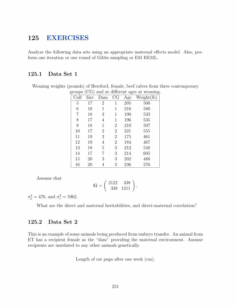
125 EXERCISES
Analyze the following data sets using an appropriate maternal effects model. Also, per-form one iteration or one round of Gibbs sampling or EM REML.
125.1 Data Set 1
Weaning weights (pounds) of Hereford, female, beef calves from three contemporarygroups (CG) and at different ages at weaning.
Calf Sire Dam CG Age Weight(lb)5 17 2 1 205 5006 18 1 1 216 5807 18 3 1 190 5338 17 4 1 196 5359 18 1 2 210 50710 17 2 2 221 55511 19 3 2 175 46112 19 4 2 184 46713 18 5 3 212 54814 17 7 3 214 60515 20 3 3 202 48016 20 4 3 236 576
Assume that
G =
(2122 338338 1211
),
σ2p = 476, and σ2
e = 5962.
What are the direct and maternal heritabilities, and direct-maternal correlation?
125.2 Data Set 2
This is an example of some animals being produced from embryo transfer. An animal fromET has a recipient female as the “dam” providing the maternal environment. Assumerecipients are unrelated to any other animals genetically.
Length of rat pups after one week (cm).
251

Pup Sire Dam Sex ET Length5 1 3 No M 7.36 1 3 Yes F 6.57 2 4 No F 7.58 2 4 No M 8.79 2 4 Yes M 9.4
Assume that
G =
(0.05 −0.01−0.01 0.02
),
σ2p = 0.014, and σ2
e = 0.12.
What are the direct and maternal heritabilities, and direct-maternal correlation?
252

Random Regression Models
126 Introduction
All biological creatures grow and perform over their lifetime. Traits that are measured atvarious times during that life are known as longitudinal data. Examples are body weights,body lengths, milk production, feed intake, fat deposition, and egg production. On abiological basis there could be different genes that turn on or turn off as an animal agescausing changes in physiology and performance. Also, an animal’s age can be recorded inyears, months, weeks, days, hours, minutes, or seconds, so that, in effect, there could bea continuum or continuous range of points in time when an animal could be observed fora trait. These traits have also been called infinitely dimensional traits.
Take body weight on gilts from a 60-day growth test as an example.
Animal Days on Test10 20 30 40 50 60
1 42 53 60 72 83 942 30 50 58 68 76 853 38 44 51 60 70 77
SD 1.6 3.7 3.9 5.0 5.3 5.6
The differences among the three animals increase with days on test as the gilts becomeheavier. As the mean weight increases, so also the standard deviation of weights increases.The weights over time could be modeled as a mean plus covariates of days on test and dayson test squared. Depending on the species and trait, perhaps a cubic or spline functionwould fit the data better. The point is that the means can be fit by a linear model witha certain number of parameters.
127 Multiple Trait Approach
The data presented in the previous table have typically been analyzed such that theweights at each day on test are different traits. If t is the day on test, i.e. 10, 20, 30, 40,50, or 60, then a model for any one of the weights could be
yt = Xbt + at + et,
which is just a simple, single record, animal model. Analyses are usually done so thatthe genetic and residual variances and covariances are estimated among the six weights.
253

Suppose that an estimate of the genetic variances and covariances was
G =
2.5 4.9 4.6 4.6 4.3 4.04.9 13.5 12.1 12.3 11.9 10.74.6 12.1 15.2 14.5 14.6 12.54.6 12.3 14.5 20.0 19.0 16.94.3 11.9 14.6 19.0 25.0 20.34.0 10.7 12.5 16.9 20.3 30.0
.
Let the residual covariance matrix be
R =
3.8 7.4 6.9 6.8 6.4 6.07.4 20.3 18.2 18.4 17.9 16.16.9 18.2 22.8 21.8 21.9 18.86.8 18.4 21.8 30.0 28.5 25.46.4 17.9 21.9 28.5 37.5 30.56.0 16.1 18.8 25.4 30.5 45.0
.
Assuming a model with only an intercept, and that the three animals are unrelated, then
(X Z) =
1 1 0 01 0 1 01 0 0 1
⊗ I6,
where the identity is of order 6 and ⊗ is the direct product operator. The observationswould be ordered by days on test within animals, i.e.,
y′ =(
42 53 60 72 83 94 · · · 60 70 77).
The resulting MME would be of order 24 by 24, and the solutions would be as follows.
Days onTest Mean Animal 1 Animal 2 Animal 310 36.67 2.10 -2.61 0.5120 49.00 1.57 0.45 -2.0230 56.33 1.48 0.64 -2.1240 66.67 2.21 0.39 -2.6050 76.33 2.72 -0.24 -2.4860 85.33 3.48 -0.16 -3.32
Animal 1 clearly grew faster than the other two animals and its superiority grewlarger with time. Animals 2 and 3 switched rankings after the first 10 days, and Animal 3was the slower growing animal. The estimates for the mean give an average growth curvefor the 3 animals.
254

A multiple trait approach may be appropriate here because every animal was weighedon exactly the same number of days on test throughout the trial. However, suppose theanimals were of different ages at the start of test, and suppose that instead of days ontest, the ages for each weight were given. Assume at start of test that Animal 1 was 18days old, Animal 2 was 22, and Animal 3 was 25. The multiple trait model could includea factor (classification or covariable) to account for different starting ages. The differencesobserved at any point in time could be due to the ages of the animals rather than just onthe number of days on test. The analysis shown above would have an implied assumptionthat all animals began the test at the same age.
128 Covariance Functions
Let the example data be as shown below, allowing for the different ages at each test.Note that the ages range from 28 days to 85 days, and that none of the animals were everweighed at exactly the same age.
Animal 1 Animal 2 Animal 3Age Wt Age Wt Age Wt28 42 32 30 35 3838 53 42 50 45 4448 60 52 58 55 5158 72 62 68 65 6068 83 72 76 75 7078 94 82 85 85 77
Kirkpatrick et al.(1991) proposed the use of covariance functions for longitudinal dataof this kind. A covariance function (CF) is a way to model the variances and covariancesof a longitudinal trait. Orthogonal polynomials are used in this model and the user mustdecide the order of fit that is best. Legendre polynomials (1797) are the easiest to apply.
To calculate Legendre polynomials, first define
P0(x) = 1, and
P1(x) = x,
then, in general, the n+ 1 polynomial is described by the following recursive equation:
Pn+1(x) =1
n+ 1((2n+ 1)xPn(x)− nPn−1(x)) .
These quantities are ”normalized” using
φn(x) =(
2n+ 1
2
).5Pn(x).
255

This gives the following series,
φ0(x) =(
1
2
).5P0(x) = .7071
φ1(x) =(
3
2
).5P1(x)
= 1.2247x
P2(x) =1
2(3xP1(x)− 1P0(x))
φ2(x) =(
5
2
).5(3
2x2 − 1
2)
= −.7906 + 2.3717x2,
and so on. The first six can be put into a matrix, Λ, as
Λ′ =
.7071 0 0 0 0 00 1.2247 0 0 0 0
−.7906 0 2.3717 0 0 00 −2.8062 0 4.6771 0 0
.7955 0 −7.9550 0 9.2808 00 4.3973 0 −20.5206 0 18.4685
.
Now define another matrix, M, as a matrix containing the polynomials of standardizedtime values. Legendre polynomials are defined within the range of values from -1 to +1.Thus, ages or time periods have to be standardized (converted) to the interval between-1 to +1. The formula is
q` = −1 + 2(t` − tmintmax − tmin
).
Let the minimum starting age for pigs on test be 15 days and the maximum starting agebe 28 days, then the maximum age at end of test was 88 days. Thus, tmin = 25 = (15+10)and tmax = 88 = (28 + 60).
The matrix G was based on weights taken on pigs that were all 21 days of age atstart of test. The table below shows the ages and standardized time values for the sixweigh dates.
Days on Age StandardizedTest Value10 31 -1.00020 41 -.60030 51 -.20040 61 .20050 71 .60060 81 1.000
256

Therefore,
M =
1 −1 1 −1 1 −11 −.600 .360 −.216 .130 −.0781 −.200 .040 −.008 .002 −.0001 .200 .040 .008 .002 .0001 .600 .360 .216 .130 .0781 1 1 1 1 1
.
This gives
Φ = MΛ,
=
.7071 −1.2247 1.5811 −1.8708 2.1213 −2.3452
.7071 −.7348 .0632 .6735 −.8655 .3580
.7071 −.2449 −.6957 .5238 .4921 −.7212
.7071 .2449 −.6957 −.5238 .4921 .7212
.7071 .7348 .0632 −.6735 −.8655 −.3580
.7071 1.2247 1.5811 1.8708 2.1213 2.3452
.
which can be used to specify the elements of G as
G = ΦHΦ′
= M(ΛHΛ′)M′
= MTM′.
Note that Φ, M, and Λ are matrices defined by the Legendre polynomial functions andby the standardized time values and do not depend on the data or values in the matrixG. Therefore, it is possible to estimate either H or T,
H = Φ−1GΦ−T ,
=
27.69 5.29 −1.95 0.05 −1.17 0.525.29 4.99 0.42 −0.25 −0.30 −0.75−1.95 0.42 1.51 0.20 −0.33 −0.07
0.05 −0.25 0.20 1.19 0.06 −0.71−1.17 −0.30 −0.33 0.06 0.58 0.15
0.52 −0.75 −0.07 −0.71 0.15 1.12
,
and
T = M−1GM−T
=
16.44 6.48 −5.93 −11.49 −0.93 10.026.48 49.87 −2.05 −155.34 1.44 111.23−5.93 −2.05 57.71 28.62 −50.06 −25.73−11.49 −155.34 28.62 635.49 −26.91 −486.90−0.93 1.44 −50.06 −26.91 49.80 26.4910.02 111.23 −25.73 −486.90 26.49 382.79
.
257

Why orthogonal polynomials? Convert T and H to correlation matrices.
Tcor =
1.00 .23 −.19 −.11 −.03 .13.23 1.00 −.04 −.87 .03 .81−.19 −.04 1.00 .15 −.93 −.17−.11 −.87 .15 1.00 −.15 −.99−.03 .03 −.93 −.15 1.00 .19.13 .81 −.17 −.99 .19 1.00
,
and
Hcor =
1.00 .45 −.30 .01 −.29 .09.45 1.00 .15 −.10 −.17 −.32−.30 .15 1.00 .15 −.36 −.05.01 −.10 .15 1.00 .07 −.62−.29 −.17 −.36 .07 1.00 .19.09 −.32 −.05 −.62 .19 1.00
.
The largest absolute correlation in T was .99, while the largest absolute correlation inH was only .62. Orthogonal polynomials tend to reduce the correlations between esti-mated regression coefficients. This is advantageous when trying to estimate H by REMLor Bayesian methods, because the estimates would converge faster to the maximum orappropriate posterior distribution than trying to estimate T. The matrix T actually hadfour correlations greater than 0.80 in absolute value, while H had none. There are otherkinds of orthogonal polynomials, but Legendre polynomials are probably the easiest tocalculate and utilize.
H can be used to calculate the covariance between any two days on test between 10and 60 days. To compute the covariance between days 25 and 55, calculate the Legendrepolynomial covariates as in calculating a row of Φ. The standardized time values for days25 and 55 are -0.4 and 0.8, respectively. The Legendre polynomials (stored in L are
L =
(.7071 −.4899 −.4111 .8232 −.2397 −.6347.7071 .9798 .7273 .1497 −.4943 −.9370
).
Then the variances and covariance for those two ages are
LHL′ =
(14.4226 13.737013.7370 28.9395
).
Thus, the genetic correlation between days 25 and 55 is 0.67. The same calculations couldbe repeated for the residual variance-covariance matrix. Let
S = Φ−1RΦ−T ,
=
41.57 7.94 −2.91 0.11 −1.76 0.767.94 7.45 0.62 −0.41 −0.44 −1.07−2.91 0.62 2.29 0.31 −0.52 −0.12
0.11 −0.41 0.31 1.76 0.08 −1.04−1.76 −0.44 −0.52 0.08 0.88 0.24
0.76 −1.07 −0.12 −1.04 0.24 1.64
,
258

then the residual variances and covariances for days 25 and 55 would be
LSL′ =
(21.6645 20.616620.6166 43.3442
).
128.1 Reduced Orders of Fit
Although the order of G in the previous example was six and polynomials of standardizedages to the fifth power were used to derive the covariance functions, perhaps only squaredor cubed powers are needed to adequately describe the elements of G. That is, find Φ∗
such that it is rectangular and H∗ has a smaller order, m < k, but still
G = Φ∗H∗Φ∗′.
To determine H∗, first pre-multiply G by Φ∗′
and post-multiply that by Φ∗ as
Φ∗′GΦ∗ = Φ∗
′(Φ∗H∗Φ∗
′)Φ∗
= (Φ∗′Φ∗)H∗(Φ∗
′Φ∗).
Now pre- and post- multiply by the inverse of (Φ∗′Φ∗) = P to determine H∗,
H∗ = P−1Φ∗′GΦ∗P−1.
To illustrate, let m = 3, then
Φ∗ =
.7071 −1.2247 1.5811
.7071 −.7348 .0632
.7071 −.2449 −.6957
.7071 .2449 −.6957
.7071 .7348 .0632
.7071 1.2247 1.5811
,
and
Φ∗′Φ∗ =
3.0000 0.0000 1.34150.0000 4.1997 0.00001.3415 0.0000 5.9758
,
(Φ∗′Φ∗)−1 =
.3705 .0000 −.0832.0000 .2381 .0000−.0832 .0000 .1860
.Also,
Φ∗′GΦ∗ =
220.2958 78.0080 61.444978.0080 67.5670 44.970761.4449 44.9707 50.5819
.259

The matrix H∗ is then 26.8082 5.9919 −2.91225.9919 3.8309 .4468−2.9122 .4468 1.3730
.What order of reduced fit is sufficient to explain the variances and covariances in G?
Kirkpatrick et al.(1990) suggested looking at the eigenvalues of the matrix H from a fullrank fit. Below are the values. The sum of all the eigenvalues was , and also shown is thepercentage of that total.
HEigenvalue Percentage
29.0357 .78314.2922 .11581.8161 .04901.3558 .0366.5445 .0147.0355 .0010
The majority of change in elements in G is explained by a constant, and by a linearincrement. Both suggest that a quadratic function of the polynomials is probably suffi-cient. Is there a way to statistically test the reduced orders of fit to determine which issufficient? A goodness of fit statistic is e′e where
e = g − g
and g is a vector of the half-stored elements of the matrix G, i.e.,
g′ =(g11 g12 · · · g16 g22 · · · g66
).
A half-stored matrix of order k has k(k + 1)/2 elements. For k = 6 there are 21 values.Likewise, g is a vector of half stored elements of the matrix Φ∗H∗Φ∗
′. Although this matrix
also has 21 values, because M has only m < k columns, the number of independent valuesis m(m+ 1)/2. For m = 3 this number is 6.
The test statistic, e′e, has a Chi-square distribution with k(k + 1)/2 −m(m + 1)/2degrees of freedom. In the example with m = 3,
Φ∗H∗Φ∗′=
3.9622 4.7467 5.2006 5.3239 5.1165 4.57864.7467 8.9493 11.4058 12.1162 11.0804 8.29865.2006 11.4058 15.2402 16.7038 15.7966 12.51865.3239 12.1162 16.7038 19.0868 19.2650 17.23865.1165 11.0804 15.7966 19.2650 21.4857 22.45864.5786 8.2986 12.5186 17.2386 22.4586 28.1786
,
260

and the residuals (differences from the original G) are
−1.4622 .1533 −.6006 −.7239 −.8165 −.5786.1533 4.5507 .6942 .1838 .8196 2.4014−.6006 .6942 −.0402 −2.2038 −1.1966 −.0186−.7239 .1838 −2.2038 .9132 −.2650 −.3386−.8165 .8196 −1.1966 −.2650 3.5143 −2.1586−.5786 2.4014 −.0186 −.3386 −2.1586 1.8214
,
so that the goodness of fit statistic is
e′e = 59.3476,
with 21-6=15 degrees of freedom.
Is a fit of order 3 poorer than a fit of order 5? An F-statistic is possible by taking thedifference in the goodness of fit statistics, divided by an estimate of the residual variance.The residual variance is estimated from a fit of order k− 1 or in this case of order 5. Thegoodness of fit statistic for order 5 was 7.2139 with 21-15=6 degrees of freedom. Hencethe residual variance is
σ2 = 7.2139/6 = 1.2023.
The F-statistic to test if a fit of order 3 is different from a fit of order 5 is
F =(e′em=3 − e′em=5)/(15− 6)
σ2
=(59.3476− 7.2139)/9
1.2023= 5.7926/1.2023 = 4.8180,
with (9,6) degrees of freedom. The table F-value at the (P = .05) level is 4.10. Thus, thedifference is significant, and a fit of order 5 is better than a fit of order 3.
261

129 Basic Structure of RRM
Random regression models have a basic structure that is similar in most applications. Asimplified RRM for a single trait can be written as
yijkn:t = Fi + g(t)j + r(a, x,m1)k + r(pe, x,m2)k + eijkn:t,
where
yijkn:t is the nth observation on the kth animal at time t belonging to the ith fixed factorand the jth group;
Fi is a fixed effect that is independent of the time scale for the observations, such as acage effect, a location effect or a herd-test date effect;
g(t)j is a function or functions that account for the phenotypic trajectory of the averageobservations across all animals belonging to the jth group;
r(a, x,m1)k =∑m1`=0 ak`xijk:` is the notation adopted for a random regression function. In
this case, a denotes the additive genetic effects of the kth animal, x is the vector oftime covariates, and m1 is the order of the regression function. So that xijk:` arethe covariables related to time t, and ak` are the animal additive genetic regressioncoefficients to be estimated;
r(pe, x,m2)k =∑m2`=0 pk`xijk:` is a similar random regression function for the permanent
environmental (pe) effects of the kth animal; and
eijkn:t is a random residual effect with mean null and with possibly different variances foreach t or functions of t.
The function, g(t)j, can be either linear or nonlinear in t. Such a function is necessaryin a RRM to account for the phenotypic relationship between y and the time covariables(or other types of covariables that could be used in a RRM). In a test day model, g(t)jaccounts for different lactation curve shapes for groups of animals defined by years ofbirth, parity number, and age and season of calving within parities, for example. Withgrowth data, g(t)j accounts for the growth curve of males or females of breed X or breedY from young or old dams.
If the shape of the phenotypic relationship is not known or is nonlinear, then g(t)jcould be a set of classification variables. Classification variables take up more degreesof freedom and require a large number of observations per level, but they do not forcethe user to explicitly define the shape of the trajectory. A mathematical function, onthe other hand, does not use many degrees of freedom and gives a smooth trajectoryover time regardless of the number of observations. The choice of classification variables
262

or mathematical function is up to the researcher. If data are very numerous, and themathematical function fits the data well, then either approach will generally lead to thesame results. The phenotypic relationships, g(t)j, are important to a RRM analysis anddeserve care and effort in their correct specification.
The random regressions are intended to model the deviations around the phenotypictrajectories. The pattern of variation may be very different in shape or appearance fromthe phenotypic relationships, and may be more simple than g(t)j. Orthogonal polynomialsof standardized units of time have been recommended as covariables (Kirkpatrick et al.,1990). Orthogonal polynomials have computational advantages. The primary generaladvantage is the reduced correlations among the estimated coefficients. A standardizedunit of time, w, ranges from -1 to +1, and is derived as
w =2 ∗ (t− tmin)
(tmax − tmin)− 1,
where tmin is the earliest date (or the youngest age) and tmax is the latest date (or oldestage) represented in the data. The order of the orthogonal polynomials would be m1 andm2, i.e. the highest power of polynomial. Note that m1 and m2 do not need to be equal,but often (for simplicity of computing) they are chosen to be the same. Meyer(2000)and Pool et al. (2000), for example, compared many RRM models with different ordersof orthogonal polynomials for the genetic and pe effects. Several types of orthogonalpolynomials are available, but Legendre polynomials have been utilized (Kirkpatrick etal., 1990). The first 6 Legendre polynomial functions of standardized units of time aregiven in Table 1. Thus, if w = −0.2, then the covariables that would go into the model(for order equal to 5) are shown in the last column of Table 1. Covariables based uponorthogonal polynomials are small numbers that reduce problems with rounding errors, andthey provide relatively small correlations between the estimated regression coefficients.
The residual variance should not be assumed to be constant from tmin to tmax. Theresidual effect is also known as a temporary environmental effect. Changes in residualvariance might be predictable depending on the trajectory of the phenotypic data. Forexample, if RRM were being applied to growth data, weights may increase linearly withage, and the variance of weights may increase quadratically with age. Thus, the residualvariance would be expected to increase in a similar manner as the phenotypic variance.Residual variances can be fit with a function of t, or assumed to have an autoregressivestructure, or can be grouped into intervals having equal variance within the intervals.Research in this area is needed.
In matrix notation the RRM is
y = Xb + Z1a + Z2p + e,
where b contains Fi and g(t)j effects, a contains m1 + 1 additive genetic regression coeffi-cients for each animal, p contains m2 + 1 permanent environmental regression coefficientsfor each animal with data, and e contains the temporary environmental effects. Also,
263

V ar
ape
=
A⊗G 0 00 I⊗P 00 0 R
,where G is the variance-covariance matrix of the additive genetic random regression coeffi-cients of order m1+1; P is the variance-covariance matrix of the permanent environmentalrandom regression coefficients of order m2 + 1; and R is a diagonal matrix of temporaryenvironmental variances which could vary depending on t, or R could be block diagonalwith an autocorrelation structure for each animal’s records. The mixed model equations(MME) are represented as
X′R−1X X′R−1Z1 X′R−1Z2
Z′1R−1X Z′1R
−1Z1 + A−1 ⊗G−1 Z′1R−1Z2
Z′2R−1X Z′2R
−1Z1 Z′2R−1Z2 + I⊗P−1
b
ap
=
X′R−1yZ′1R
−1yZ′2R
−1y
.Assumptions about the distributions of y and other random variables are not necessaryto derive best linear unbiased predictors (BLUP)(Goldberger, 1962; Henderson, 1984) orthe MME, but when y is normally distributed then BLUP is also BLP if the model iscorrect and variances and covariances are known. In order to estimate the elements ofG, P, and R via Bayesian methods or restricted maximum likelihood, then normality ofthe random variables must be assumed (See for example Jamrozik and Schaeffer, 1997).This paper will concentrate on the applications of RRM and not on the estimation of(co)variance parameters, nor on the computational details of estimating (co)variances orsolving mixed model equations. Some of the applications in this paper have applied RRMto discrete data, and therefore, a BLUP analysis would not be optimum. However, thepresentation of these ideas may stimulate others to find better solutions.
130 Example Data Analysis By RRM
Below are the data structure and pedigrees of four dairy cows. Given is the age at whichthey were observed for a trait during four visits to one herd.
Age, Obs. at VisitCow Sire Dam Visit 1 Visit 2 Visit 3 Visit 4
1 7 5 22,224 34,236 47,2392 7 6 30,244 42,247 55,241 66,2443 8 5 28,224 40,2424 8 1 20,220 33,234 44,228
264

The model equation might be
yjik:t = Vj + b0 + b1(A) + b2(A)2
+(ai0z0 + ai1z1 + ai2z2)
+(pi0z0 + pi1z1 + pi2z2) + ejik:t
where
Vj is a random contemporary group effect which is assumed to follow a normal distri-bution with mean 0 and variance, σ2
c = 4.
b0, b1, and b2 are fixed regression coefficients on (A) = age and age squared whichdescribes the general relationship between age and the observations,
ai0, ai1, and ai2 are random regression coefficients for animal i additive genetic effects,assumed to follow a multivariate normal distribution with mean vector null andvariance-covariance matrix, G,
pi0, pi1, and pi2 are random regression coefficients for animal i permanent environmentaleffects, assumed to follow a multivariate normal distribution with mean vector nulland variance-covariance matrix, P,
z0, z1, and z2 are the Legendre polynomials based on standardized ages and derived asindicated earlier. The minimum age was set at 18 and the maximum age was set at68 for calculating the Legendre polynomials.
and ejik is a temporary residual error term assumed to follow a normal distribution withmean 0 and variance, σ2
e = 9. In this example, the residual variance is assumed tobe constant across ages.
The model in matrix notation is
y = Xb + Wv + Za + Zp + e,
where
X =
1 22 4841 30 9001 28 7841 34 11561 42 17641 40 16001 20 4001 47 22091 55 30251 33 10891 66 43561 44 1936
, y =
224244224236247242220239241234244228
, W =
1 0 0 01 0 0 01 0 0 00 1 0 00 1 0 00 1 0 00 1 0 00 0 1 00 0 1 00 0 1 00 0 0 10 0 0 1
,
265

and
Z =
.7071 −1.0288 .8829 0 0 0 0 0 0 0 0 00 0 0 .7071 −.6369 −.1493 0 0 0 0 0 00 0 0 0 0 0 .7071 −.7348 .0632 0 0 0
.7071 −.4409 −.4832 0 0 0 0 0 0 0 0 00 0 0 .7071 −.0490 −.7868 0 0 0 0 0 00 0 0 0 0 0 .7071 −.1470 −.7564 0 0 00 0 0 0 0 0 0 0 0 .7071 −1.1268 1.2168
.7071 .1960 −.7299 0 0 0 0 0 0 0 0 00 0 0 .7071 .5879 −.2441 0 0 0 0 0 00 0 0 0 0 0 0 0 0 .7071 −.4899 −.41110 0 0 .7071 1.1268 1.2168 0 0 0 0 0 00 0 0 0 0 0 0 0 0 .7071 .0490 −.7868
.
In order to reduce rounding errors the covariates of age for the fixed regressions can beforced to have a mean of approximately zero by subtracting 38 from all ages and 1642from all ages squared. Then
X =
1 −16 −11581 −8 −7421 −10 −8581 −4 −4861 4 1221 2 −421 −18 −12421 9 5671 17 13831 −5 −5531 28 27141 6 294
.
The mixed model equations that need to be constructed to provide estimated breedingvalues are as follows;
X′X X′W X′Z 0 X′ZW′X W′W + I 9
4 W′Z 0 W′ZZ′X Z′W Z′Z + Ann ⊗G−1 Anb ⊗G−1 Z′Z0 0 Abn ⊗G−1 Abb ⊗G−1 0Z′X Z′W Z′Z 0 Z′Z + I⊗P−1
bcan
ab
p
=
X′yW′yZ′y0
Z′y
.
The entire MME can not be presented, but parts of the MME are given below.
W′W =
3 0 0 00 4 0 00 0 3 00 0 0 2
,
W′X =
3 −34 −27584 −16 −16483 21 13972 34 3008
,
266

X′X =
12 5 −15 1995 166, 883−1 166, 883 14, 415, 319
,
Z′Z is composed of the following four blocks of order 3, for the four animals withrecords;
Animal 1
1.5 −.9006 −.2335−.9006 1.2912 −.8383−.2335 −.8383 1.5457
,
Animal 2
2 .7275 .0259.7275 2.0233 1.3612.0259 1.3612 2.1815
,
Animal 3
1 −.6235 −.4902−.6235 .5615 .0648−.4902 .0648 .5761
,
Animal 4
1.5 −1.1085 .0134−1.1085 1.5121 −1.2082.0134 −1.2082 2.2687
.and Z′X is
Z′X =
2.1213 −7.7781 −761.5467−1.2737 19.9884 1516.7598−.3302 −18.7627 −1201.4162.8284 28.9911 2458.58671.0288 46.4439 4337.8027.0366 27.9679 2979.5959
1.4142 −5.6568 −636.3900−.8818 7.0540 636.6324−.6932 −2.1448 −22.45682.1213 −12.0207 −1061.3570−1.5677 23.0259 1684.8063.0189 −24.5677 −1515.2470
.
The right hand sides of the MME are
X′y =
28232070
68, 064
,
267

W′y =
692945714472
,and
Z′y =
494.2629−287.6596−90.7117690.1296249.1165
7.3023329.5086−200.1692−168.8920
482.2422−351.3606−7.8918
.
The variance-covariance matrices of the additive and permanent environmental effectsneed to be known for BLUP. Normally, these are not well known and must be estimatedsimultaneously with the other effects of the model. Let
G =
94.0000 −3.8500 .03098−3.8500 1.5000 −.0144.03098 −.0144 .0014
,and
P =
63.0000 −2.1263 .0447−2.1263 .5058 −.00486.0447 −.00486 .0005
.The solutions to MME are
b′ =(
234.9797 1.4670 −.01399),
c′ =
−.86301.2885.1443−.5698
.Let the solutions for the animal additive genetic random regression coefficients be pre-sented in tabular form as follows.
268

Animal a0 a1 a2
1 -2.021529 .175532 -.0026962 5.751601 -2.139115 .0258483 -2.474456 2.554412 -.0292694 -5.376687 -.370873 .0021745 -1.886714 1.464975 -.0169636 3.333268 -1.065525 .0130477 1.503398 -1.081654 .0125558 -2.948511 .681643 -.008633
Similarly, the solutions for the animal permanent environmental random regressioncoefficients can be given in tabular form.
Animal p0 p1 p2
1 -.296786 .246946 -.0025212 3.968256 -.730659 .0094303 -.834765 .925329 -.0081644 -4.505439 -.441805 .001257
The problem is to rank the animals for selection purposes. If animals are ranked onthe basis of a0, then animal 2 would be the highest (if that was desirable). If ranked onthe basis of a1, then animal 3 would be the highest, and if ranked on the basis of a2,then animal 2 would be the highest. To properly rank the animals, an EBV at differentages could be calculated, and then these could be combined with appropriate economicweights. Calculate EBVs for 24, 36, and 48 mo of age, and use economic weights of 2, 1,and .5, respectively, for the three EBVs. A Total Economic Value can be calculated as
TEV = 2 ∗ EBV(24) + 1 ∗ EBV(36) + .5 ∗ EBV(48).
The Legendre polynomials for ages 24, 36, and 48 mo are given in the rows of the followingmatrix L,
L =
.7071 −.8328 .3061.7071 −.3429 −.6046.7071 .2449 −.6957
.The results are shown in the following table.
269

Animal EBV(24) EBV(36) EBV(48) TEV1 -1.58 -1.49 -1.38 -5.332 5.86 4.78 3.53 18.263 -3.89 -2.61 -1.10 -10.934 -3.49 -3.68 -3.89 -12.615 -2.56 -1.83 -.96 -7.436 3.25 2.71 2.09 10.257 1.97 1.43 .79 5.768 -2.66 -2.31 -1.91 -8.58
The animal with the highest TEV was animal 2. All animals ranked rather similarlyat each age on their EBVs. Rankings of animals could change with age. Thus, the patternof growth could be changed one that is desirable.
Estimation of the residual variance is
σ2e = (y′y − b′X′y − c′W′y − a′nM
′y − p′M′y)/(N − r(X)),
where
y′y = 665, 035,
β′W′y = 664902.89,
N − r(X) = 12− 3 = 9,
σ2e = 14.6788.
131 EXERCISES
1. A biologist studied chipmunks in southern Ontario. He planted small TV camerasinside four nests of chipmunks. The territories of the occupants of the four nestsdid not overlap. With the cameras he had students monitor the nests for a day atseveral times during the summer and fall. Students counted the number of nutsthat were collected and stored in the nest on a given day during a set 8 hour period.Below are the observations on the four nests for various days of the year.
Number of nuts collected in 8 hours.Day of Year Nest Number of Nuts Day of Year Nest Nuts
123 1 25 161 1 11124 2 37 155 2 14127 3 16 153 3 9129 4 42 151 4 12192 1 13 225 1 38194 2 15 227 2 29198 3 10 233 3 37200 4 16 246 4 44
270

(a) Write a complete random regression model for these data, including the as-sumptions and limitations.
(b) Compute a simple 4 by 4 phenotypic covariance matrix for the four nest sites.Then use covariance functions and tests to determine the appropriate order fora random regression model, and to obtain initial covariance matrices for themodel.
(c) Apply the random regression model to the data, and plot the differences be-tween the nests.
271

Multiple Traits
132 Introduction
Animals are commonly observed for more than one trait because many traits affect overallprofitability. A multiple trait (MT) model is one in which two or more traits are ana-lyzed simultaneously in order to take advantage of genetic and environmental correlationsbetween traits.
Low Heritability Traits: MT models are useful for traits where the differencebetween genetic and residual correlations are large ( e.g. greater than 0.5 difference ) orwhere one trait has a much higher heritability than the other trait. EBVs for traits withlow heritability tend to gain more in accuracy than EBVs for traits with high heritability,although all traits benefit to some degree from the simultaneous analysis.
Culling: Another use of MT models is for traits that occur at different times in thelife of the animal, such that culling of animals results in fewer observations on animals fortraits that occur later in life compared to those at the start. Consequently, animals whichhave observations later in life tend to have been selected based on their performance forearlier traits. Thus, analysis of later life traits by themselves could suffer from the effectsof culling bias, and the resulting EBV could lead to errors in selecting future parents.An MT analysis that includes all observations on an animal upon which culling decisionshave been based, has been shown to account, to some degree, for the selection that hastaken place.
MT models do not offer great increases in accuracy for cases where heritabilities oftraits are similar in magnitude, where both genetic and residual correlations are relativelythe same magnitude and sign, or where every animal is measured for all traits. However,if culling bias may exist, then an MT analysis should be performed even if the parametersare similar. An MT analysis relies on the accuracy of the genetic and residual correlationsthat are assumed.
If the parameter estimates are greatly different from the underlying, unknown truevalues, then an MT analysis could do as much harm as it might do good.
Computer programs are more complicated, require more memory and disk storagefor MT analyses. Verification of results might be more complicated. These have to bebalanced against the benefits of an MT analysis. If culling bias is the main concern, thenan MT model must be used regardless of the costs or no analysis should be done at all,except for the traits not affected by culling bias.
272
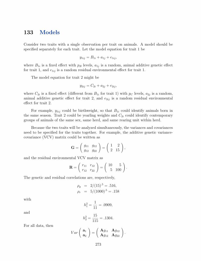
133 Models
Consider two traits with a single observation per trait on animals. A model should bespecified separately for each trait. Let the model equation for trait 1 be
y1ij = B1i + a1j + e1ij,
where B1i is a fixed effect with pB levels, a1j is a random, animal additive genetic effectfor trait 1, and e1ij is a random residual environmental effect for trait 1.
The model equation for trait 2 might be
y2ij = C2i + a2j + e2ij,
where C2i is a fixed effect (different from B1i for trait 1) with pC levels, a2j is a random,animal additive genetic effect for trait 2, and e2ij is a random residual environmentaleffect for trait 2.
For example, y1ij could be birthweight, so that B1i could identify animals born inthe same season. Trait 2 could be yearling weights and C2i could identify contemporarygroups of animals of the same sex, same herd, and same rearing unit within herd.
Because the two traits will be analyzed simultaneously, the variances and covariancesneed to be specified for the traits together. For example, the additive genetic variance-covariance (VCV) matrix could be written as
G =
(g11 g12
g12 g22
)=
(1 22 15
),
and the residual environmental VCV matrix as
R =
(r11 r12
r12 r22
)=
(10 55 100
).
The genetic and residual correlations are, respectively,
ρg = 2/(15).5 = .516,
ρr = 5/(1000).5 = .158
with
h21 =
1
11= .0909,
and
h22 =
15
115= .1304.
For all data, then
V ar
(a1
a2
)=
(Ag11 Ag12
Ag12 Ag22
).
273

The structure of the residual VCV matrix over all observations can be written severalways depending on whether allowance is made for missing observations on either trait forsome animals. If all animals were observed for both traits, then
V ar
(e1
e2
)=
(Ir11 Ir12
Ir12 Ir22
).
134 Simulation of Trait Records
When simulating data for a multiple trait problem, observations for all animals for alltraits should be generated. Then one can go through the simulated data and deleteobservations to simulate a missing data situation, or selectively delete observations toimitate culling decisions. Another simplification is to assume that the model for eachtrait is the same, and then for a factor that does not belong with a given trait just makethe true values of levels for that factor and trait equal to zero. In matrix form, the modelequation for one animal would be
(y1ij
y2ij
)=
(1 0 0 00 0 1 0
)B11
B12
B21
B22
+
(0 1 0 0 0 00 0 0 0 1 0
)
C11
C12
C13
C21
C22
C23
+
(Parent Ave. Trait 1Parent Ave. Trait 2
)+ (bii)
.5LG
(RND(1)RND(2)
)
+LR
(RND(3)RND(4)
),
where LG and LR are lower triangular matrices such that
G = LGL′G
=
(1 02 (11).5
)L′G
and R = LRL′R
=
((10).5 0
(2.5).5 (97.5).5
)L′R.
Let B11 = 6.7 and B12 = 6.3 for trait 1, and because factor B is not in the modelfor trait 2, then B21 = 0 and B22 = 0. Similarly, C21 = 25, C22 = 40, and C23 = 55 fortrait 2, and because factor C is not in the model for trait 1, then C11 = 0, C12 = 0, and
274

C13 = 0. Suppose the animal is a base animal, then bii = 1 and the parent averages fortraits 1 and 2 are assumed to be zero, then the observations would be
(y1ij
y2ij
)=
(1 0 0 00 0 1 0
)6.76.300
+
(0 1 0 0 0 00 0 0 0 1 0
)
000254055
+
(Parent Ave. Trait 1=0Parent Ave. Trait 2=0
)+ (1).5
(1 02 (11).5
)(.6942−1.3027
)
+
((10).5 0(2.5).5 (97.5).5
)(−.5324−.9468
),
=
(6.7
0
)+
(0
40
)+
(.6942
−2.9322
)+
(−1.6836−10.1907
)
=
(5.7106
26.8771
).
The following data (rounded off) were simulated according to the preceeding schemeand parameters.
Animal Sire Dam B-level C-level Trait 1 Trait 21 0 0 1 1 2.3 392 0 0 1 2 2.6 393 0 0 1 3 9.8 534 0 0 1 1 4.7 45 0 0 1 2 5.5 636 1 3 2 3 2.5 647 1 4 2 2 8.4 358 1 5 2 3 8.2 419 2 3 2 1 9.0 2710 2 4 2 1 7.8 3211 2 5 2 2 2.8 4612 6 10 2 3 7.4 67
To simulate selection, assume that all animals had trait 1 observed, but any ani-mal with a trait 1 value below 3.0, then trait 2 observation was removed. Four trait 2observations were deleted, giving the results in the table below.
275

Animal Sire Dam B-level C-level Trait 1 Trait 21 0 0 1 1 2.32 0 0 1 2 2.63 0 0 1 3 9.8 534 0 0 1 1 4.7 45 0 0 1 2 5.5 636 1 3 2 3 2.57 1 4 2 2 8.4 358 1 5 2 3 8.2 419 2 3 2 1 9.0 2710 2 4 2 1 7.8 3211 2 5 2 2 2.812 6 10 2 3 7.4 67
135 HMME
Organize the data by traits within animals. With two traits there are three possibleresidual matrices per animal, i.e.,
R12 =
(10 55 100
),
R1 =
(10 00 0
),
R2 =
(0 00 100
),
depending on whether both traits, trait 1, or trait 2, respectively, were observed. In theexample data, only R12 and R1 are needed. To simplify notation, let
E12 = R−112
=1
975
(100 −5−5 10
)
=
(.102564 −.005128−.005128 .010256
),
and
E1 = R−1
=
(.1 00 0
),
E2 = R−2
=
(0 00 .01
).
276

Again, to simplify construction of the MME, pretend that both traits have the samemodel equation, so that
ytijk = Bti + Ctj + atk + etijk.
There are 2 levels of factor B, three levels of factor C, and 12 animals. For a single traitmodel this would give MME of order 17. Construct a table of order 17. The elements ofthis table will be matrices of order 2(in general, order t). Start with animal 1, then
y1 =
(2.3−
), and E1y1 =
(.230
).
Now add E1 to the boxes in the MME table as follows:
B1 B2 C1 C2 C3 a1 · · · RHSB1 E1 E1 E1 E1y1
B2
C1 E1 E1 E1 E1y1
C2
C3
a1 E1 E1 E1 E1y1
Similarly for animal 2,
y2 =
(2.6−
), and E1y2 =
(.260
).
Accumulating into the MME table gives
B1 B2 C1 C2 C3 · · · a2 RHSB1 2E1 E1 E1 E1 E1(y1 + y2)B2
C1 E1 E1 E1y1
C2 E1 E1 E1 E1y2
C3
a2 E1 E1 E1 E1y2
For animal 3,
y3 =
(9.853
), and E12y3 =
(.7333.4933
),
and the MME table becomes
277

B1 B2 C1 C2 C3 · · · a3 RHSB1 2E1 + E12 E1 E1 E12 E12 E1(y1 + y2) + E12y3
B2
C1 E1 E1 E1y1
C2 E1 E1 E1y2
C3 E12 E12 E12 E12y3
a3 E12 E12 E12 E12y3
The remaining animals are processed in the same manner. The resulting equationsare of order 34 by 34. To these A−1 ⊗ G−1 must be added to the animal by animalsubmatrix in order to form the full HMME. However, solutions for the B-factor for trait 2are not needed because the B-factor does not affect trait 2, and solutions for the C-factorfor trait 1 are not needed because the C-factor does not affect trait 1. Therefore, removerows (and columns) 2, 4, 5, 7, and 9, or if an iterative solution is being computed, thenrequire that the solutions for B21, B22, C11, C12, and C13 are always equal to zero. Thesolutions to the HMME, for this example, were
B11 = 5.0209
B12 = 6.5592
C21 = 20.0882
C22 = 49.0575
C23 = 51.9553
The animal additive genetic solutions are shown in the table below.
Animal Sire Dam Trait 1 Trait 21 0 0 -.3573 -1.67722 0 0 -.0730 1.04183 0 0 .4105 1.17074 0 0 -.0449 -1.49225 0 0 .0646 .95706 1 3 -.1033 -.14107 1 4 -.1975 -2.29838 1 5 -.1410 -.96339 2 3 .3079 1.622710 2 4 .1426 1.127311 2 5 -.1830 .641812 6 10 .1554 1.5089
The correlation between the animal additive genetic solutions for traits 1 and 2 was.74 which is greater than the .52 assumed in the original G.
278

136 Bruce Tier’s MT Trick
There is another way to construct the MME without the need of forming different inversesof R for missing traits. If a trait is missing, then that observation is assigned to its owncontemporary group in the model for that trait. In the example data there were fourmissing observations. Animal 1 would be assigned to C24, animal 2 to C25, animal 6to C26 and animal 11 to C27, respectively. In this case only trait 2 observations weremissing. If trait 1 observations were also missing, then animals would be assigned toseparate levels of factor B. In this way, only one residual VCV matrix is needed, i.e. R12.Let X represent the design matrix for fixed effects (factors B and C) for either trait. Notethe four extra columns for factor C for the animals with missing trait 2 observations.
Xb =
1 0 0 0 0 1 0 0 01 0 0 0 0 0 1 0 01 0 0 0 1 0 0 0 01 0 1 0 0 0 0 0 01 0 0 1 0 0 0 0 00 1 0 0 0 0 0 1 00 1 0 1 0 0 0 0 00 1 0 0 1 0 0 0 00 1 1 0 0 0 0 0 00 1 1 0 0 0 0 0 00 1 0 0 0 0 0 0 10 1 0 0 1 0 0 0 0
B11
B12
C21
C22
C23
C24
C25
C26
C27
.
A missing observation is replaced with zero. The resulting solutions are identical tothose given earlier, except that now there are also solutions for the single observationcontemporary groups. That is, C24 = 2.8590, C25 = .1322, C26 = 2.1189, and C27 =1.1463. These solutions do not mean anything, but must be calculated.
To prove that this trick will work, take R−1 and do a Gaussian elimination (i.e.absorption) of the row and column corresponding to the missing trait, say trait 2,(
e11 e12
e12 e22
)−(e12
e22
)(e22)−1
(e12 e22
),
=
(e11 e12
e12 e22
)−(e12(e22)−1e12 e12
e12 e22
),
=
(e11 − e12(e22)−1e12 0
0 0
).
Recall that for a matrix of order 2 that
e11 = e22/ | R |,
279

e12 = −e12/ | R |,e22 = e11/ | R |,| R | = (e11e22 − e12e12)
then
e11 − e12(e22)−1e12 = (e22 − e12(e11)−1e12)/ | R |
= e11(e22 − e12(e11)−1e12/e11(e11e22 − e12e12)
= (e11)−1
which is exactly the weight applied to records on animals with only trait 1 observed.This proof can be extended to any number of traits recorded and any number missing, bypartitioning R into (
Roo Rom
Rmo Rmm
),
where the subscript o refers to traits that were observed and m refers to traits that weremissing on an animal. Then it can be easily shown that
R−1oo = Roo −Rom(Rmm)−1Rmo.
This trick is not very practical, for example, when one trait has 1 million observa-tions and trait 2 has only 100,000 observations, then there would be 900,000 extra singleobservation subclasses created for trait 2. However, if the percentages of missing obser-vations are relatively small, or if many traits are being considered, then pretending allobservations are present may make programming easier.
137 Estimation of Covariance Matrices
Derivative free REML is one option for estimating variances and covariances in a multi-trait situation. The EM algorithm is not suitable due to the requirement for the traces ofinverse elements that are needed. Even DF REML takes considerably more time as thenumber of parameters to be estimated increases.
Another option is the Bayesian approach, where operations are performed in t di-mensions, for t being the number of traits. Thus, for a solution to the MME, the t × 1vector for any one fixed effect, for example, would be
βi = (X′iR−1Xi)
−1X′iR−1(yi −W−iβ−i),
thenβi = βi + Lv,
280

whereLL′ = (X′iR
−1Xi)−1,
and v is a t×1 vector of random normal deviates. Similar formulas can be derived for therandom factors of the model. The conditional distributions for these factors are assumedto be normally distributed.
If ai is the q × 1 vector of animal solutions for trait i, then form
U =(
a1 a2 · · · at),
followed bySa = (U′A−1U + νaGa),
which is then inverted and a Cholesky decomposition is applied to the inverse, i.e.
LaL′a = S−1
a ,
where La is supplied to a Wishart distribution random number generator to give a newsample matrix for the inverse of the additive genetic variances and covariances.
A difficult part of a multiple trait analysis, when missing traits are possible, is thecalculation of the appropriate residual matrix of sums of squares and cross products. Theresidual effect for any one trait is
eti = yti −w′iβt,
and for a particular animal, k,
resk =(
e′o e′m),
where the subscripts o and m refer to observed and missing, respectively, and wheree′m = 0′. In order to calculate the correct sum of squares and crossproducts of theresiduals for REML or the Bayesian approach, a prediction of em is needed. This can beeasily done by
res′k∗ =
(Roo Rom
Rmo Rmm
)(R−1oo 0
0 0
)(eo0
).
For the first animal in the example data, for example, the estimated residual for trait 1was -2.363638, then
res′1∗ =
(10 55 100
)(110
00 0
)(−2.363638
0
),
=
(1 0.5 0
)(−2.363638
0
),
=
(−2.363638−1.181819
).
281

If you use Bruce Tier’s MME with the single observation contemporary groups formissing trait observations, then the residuals can be calculated directly by (y−Wβ) usingzero as the observation for the missing traits and using the solutions for the single obser-vation contemporary groups. This gives the exact same residual estimates as the abovemethodology. Therefore, Tier’s approach is handy for the Gibb’s sampling algorithm.
Once the residuals are calculated for all animals with records, then calculate
res′k∗resk∗,
and sum across N animals. Then let
Se = (N∑k=1
(res′k∗resk∗) + νeRe),
which is then inverted and a Cholesky decomposition is applied to the inverse, i.e.
LeL′e = S−1
e ,
where Le is supplied to a Wishart distribution random number generator to give a newsample matrix for the inverse of the residual variances and covariances.
282

138 EXERCISES
Below are data on three blood component traits (just called Trait 1, Trait 2, and Trait 3)taken on 6 mink adults. The lab technician slid on a banana peel, dropped some of theblood samples, and so some data were lost. The technician was fired for eating in the lab.
Animal Sire Dam Age(yrs) Trait 1 Trait 2 Trait 36 1 3 3 2.5 537 1 4 2 8.4 1758 1 5 3 41 1979 2 3 1 9.010 2 4 1 32 15611 2 5 2 168
Let
R =
11 5 295 97 63
29 63 944
,and
G =
0.94 1.62 −5.871.62 14.33 −11.79−5.87 −11.79 803.41
.
1. Write a model for the analysis.
2. Analyze the data with that model.
3. Rank the animals in some way.
4. Perform one iteration or one round of sampling to estimate the covariance matrices.
283

Non-Additive Animal Models
139 Non-Additive Genetic Effects
Non-additive genetic effects (or epistatic effects) are the interactions among loci in thegenome. There are many possible degrees of interaction (involving different numbers ofloci), but the effects and contributions of those interactions have been shown to diminishas the degree of complexity increases. Thus, mainly dominance, additive by additive,additive by dominance, and dominance by dominance interactions have been consideredin animal studies.
To estimate the variances associated with each type of interaction, relatives are neededthat have different additive and dominance relationships among themselves. Computationof dominance relationships is more difficult than additive relationships, but can be doneas shown in earlier notes.
If non-additive genetic effects are included in an animal model, then an assumptionof random mating is required. Otherwise non-zero covariances can arise between additiveand dominance genetic effects, which complicates the model enormously.
140 Interactions at a Single Locus
Let the model for the genotypic values be given as
Gij = µ+ ai + aj + dij,
where
µ = G.. =∑i,j
fijGij,
ai = Gi. −G..,
Gi. = Pr(A1)G11 + Pr(A2)G12,
aj = G.j −G..
G.j = Pr(A1)G12 + Pr(A2)G22,
dij = Gij − ai − aj − µ
Thus, there are just additive effects and dominance effects to be estimated at a singlelocus. A numerical example is given below.
284

Genotype Frequency ValueA1A1 f11 = 0.04 G11 = 100A1A2 f12 = 0.32 G12 = 70A2A2 f22 = 0.64 G22 = 50
Then
µ = 0.04(100) + 0.32(70) + 0.64(50) = 58.4,
G1. = 0.2(100) + 0.8(70) = 76.0,
G.2 = 0.2(70) + 0.8(50) = 54.0,
a1 = G1. − µ = 17.6,
a2 = G.2 − µ = −4.4,
d11 = G11 − a1 − a1 − µ = 6.4,
d12 = G12 − a1 − a2 − µ = −1.6,
d22 = G22 − a2 − a2 − µ = 0.4.
Now a table of breeding values and dominance effects can be completed.
Genotype Frequency Total Additive DominanceA1A1 0.04 G11 = 100 a1 + a1 = 35.2 d11 = 6.4A1A2 0.32 G12 = 70 a1 + a2 = 13.2 d12 = −1.6A2A2 0.64 G22 = 50 a2 + a2 = −8.8 d22 = 0.4
The additive genetic variance is
σ2a = 0.04(35.2)2 + 0.32(13.2)2 + 0.64(−8.8)2 = 154.88,
and the dominance genetic variance is
σ2d = 0.04(6.4)2 + 0.32(−1.6)2 + 0.64(0.4)2 = 2.56,
and the total genetic variance is
σ2G = σ2
a + σ2d
= 157.44,
= 0.04(100− µ)2 + 0.32(70− µ)2 + 0.64(50− µ)2
= 0.04(41.6)2 + 0.32(11.6)2 + 0.64(−8.4)2
= 157.44.
285

This result implies that there is a zero covariance between the additive and domi-nance deviations. This can be shown by calculating the covariance between additive anddominance deviations,
Cov(A,D) = 0.04(35.2)(6.4) + 0.32(13.2)(−1.6) + 0.64(−8.8)(0.4)
= 0
The covariance is zero under the assumption of a large, random mating population withoutselection.
141 Interactions for Two Unlinked Loci
Consider two loci each with two alleles, and assume that the two loci are on differentchromosomes and therefore unlinked. Let pA = 0.4 be the frequency of the A1 allele atlocus A, and let pB = 0.8 be the frequency of the B1 allele at locus B. Then the possiblegenotypes, their expected frequencies assuming joint equilibrium, and genotypic valueswould be as in the table below. Joint equilibrium means that each locus is in Hardy-Weinberg equilibrium and that the probabilities of the possible gametes are equal to theproduct of the allele frequencies as shown in the table below.
Possible ExpectedGametes FrequenciesA1 B1 pApB = 0.32
A1 B2 pAqB = 0.08
A2 B1 qApB = 0.48
A2 B2 qAqB = 0.12
Multiplying these gametic frequencies together, to simulate random mating gives thefrequencies in the table below. The genotypic values were arbitrarily assigned to illustratethe process of estimating the genetic effects.
286

Genotypes Frequencies GenotypicA-Locus B-locus fijk` Value,Gijk`
i, j k, `11 11 p2
Ap2B =.1024 G1111 = 108
11 12 p2A2pBqB =.0512 G1112 = 75
11 22 p2Aq
2B =.0064 G1122 = −80
12 11 2pAqAp2B =.3072 G1211 = 95
12 12 4pAqApBqB =.1536 G1212 = 5012 22 2pAqAq
2B =.0192 G1222 = −80
22 11 q2Ap
2B =.2304 G2211 = 48
22 12 q2A2pBqB =.1152 G2212 = 36
22 22 q2Aq
2B =.0144 G2222 = −100
141.1 Estimation of Additive Effects
αA1 = G1... − µG = 16.6464,
αA2 = −11.0976,
αB1 = 10.4384,
αB2 = −41.7536.
The additive genetic effect for each genotype is
aijk` = αAi + αAj + αBk + αB`
a1111 = αA1 + αA1 + αB1 + αB1,
= 16.6464 + 16.6464 + 10.4384 + 10.4384,
= 54.1696,
a1112 = 1.9776,
a1122 = −50.2144,
a1211 = 26.4256,
a1212 = −25.7664,
a1222 = −77.9584,
a2211 = −1.3184,
a2212 = −53.5104,
a2222 = −105.7024.
The additive genetic variance is then
σ2a =
∑ijk`
fijk`a2ijk` = 1241.1517.
287

141.2 Estimation of Dominance Effects
There are six conditional means to compute, one for each single locus genotype.
G11.. = Pr(B1B1)G1111 + Pr(B1B2)G1112 + Pr(B2B2)G1122,
= (.64)(108) + (.32)(75) + (.04)(−80),
= 89.92,
G12.. = 73.60,
G22.. = 38.24,
G..11 = 80.16,
G..12 = 48.96,
G..22 = −87.20.
The dominance genetic effects are given by
δAij = Gij.. − µG − αAi − αAj,
so that
δA11 = 89.92− 63.4816− 16.6464− 16.6464,
= −6.8544,
δA12 = 4.5696,
δA22 = −3.0464,
δB11 = −4.1984,
δB12 = 16.7936,
δB22 = −67.1744.
The dominance deviations for each genotype are
dijk` = δAij + δBk`,
d1111 = −11.0528,
d1112 = 9.9392,
d1122 = −74.0288,
d1211 = 0.3712,
d1212 = 21.3632,
d1222 = −62.6048,
d2211 = −7.2448,
d2212 = 13.7472,
d2222 = −70.2208.
288

The dominance genetic variance is therefore,
σ2d =
∑ijk`
fijk`d2ijk` = 302.90625.
141.3 Additive by Additive Effects
These are the interactions between alleles at different loci. There are four conditionalmeans to calculate,
G1.1. = Pr(A1B1)G1111 + Pr(A1B2)G1112
+Pr(A2B1)G1211 + Pr(A2B2)G1212,
= .32(108) + .08(75) + .48(95) + .12(50),
= 92.16,
G1..2 = 84.192,
G.21. = 61.76,
G.2.2 = 14.88.
The additive by additive genetic effect is
ααA1B1 = G1.1. − µG − αA1 − αB1 = 1.5936,
ααA1B2 = −6.3744,
ααA2B1 = −1.0624,
ααA2B2 = 4.2496.
The additive by additive deviations for each genotype are
aaijk` = ααAiBk + ααAiB` + ααAjBk + ααAjB`,
aa1111 = 6.3744,
aa1112 = −9.5616,
aa1122 = −25.4976,
aa1211 = 1.0624,
aa1212 = −1.5936,
aa1222 = −4.2496,
aa2211 = −4.2496,
aa2212 = 6.3744,
aa2222 = 16.9984.
289

The additive by additive genetic variance is
σ2aa =
∑ijk`
fijk`aa2ijk` = 27.08865.
141.4 Additive by Dominance Effects
This is the interaction between a single allele at one locus with the pair of alleles at asecond locus. There are twelve possible conditional means for twelve possible different Aby D interactions. Not all are shown,
G1.11 = Pr(A1)G1111 + Pr(A2)G1211,
= .4(108) + .6(95),
= 100.2,
G.211 = Pr(A1)G1211 + Pr(A2)G2211,
= .4(95) + .6(48),
= 66.8.
The specific additive by dominance effects are
αδA1B11 = G1.11 − µG − αA1 − 2αB1 − δB11 = 0.2064.
Finally, the additive by dominance genetic values for each genotype are
adijk` = αδAiBk` + αδAjBk` + αδBkAij + αδB`Aij,
ad1111 = −3.8784,
ad1112 = 4.7856,
ad1122 = 23.7696,
ad1211 = 2.9296,
ad1212 = −4.5664,
ad1222 = −10.3424,
ad2211 = −2.1824,
ad2212 = 3.9616,
ad2222 = 3.2256.
The additive by dominance genetic variance is
σ2ad =
∑ijk`
fijk`ad2ijk` = 17.2772.
290

141.5 Dominance by Dominance Effects
Dominance by dominance genetic effects are the interaction between a pair of alleles atone locus with another pair of alleles at a second locus. These effects are calculated asthe genotypic values minus all of the other effects for each genotype. That is,
ddijk` = Gijk` − µG − aijk` − dijk` − aaijk` − adijk`.
The dominance by dominance genetic variance is the sum of the frequencies of eachgenotype times the dominance by dominance effects squared, σ2
dd = 8.5171. The table ofall genetic effects are given below.
Genotypes fijk` Gijk` aijk` dijk` aaijk` adijk` ddijk`A-Locus B-Locus
11 11 .1024 108 54.1696 -11.0528 6.3744 -3.8784 -1.094411 12 .0512 75 1.9776 9.9392 -9.5616 4.7856 4.377611 22 .0064 -80 -50.2144 -74.0288 -25.4976 23.7696 -17.510412 11 .3072 95 26.4256 0.3712 1.0624 2.9296 0.729612 12 .1536 50 -25.7664 21.3632 -1.5936 -4.5664 -2.918412 22 .0192 -80 -77.9584 -62.6048 -4.2496 -10.3424 11.673622 11 .2304 48 -1.3184 -7.2448 -4.2496 -2.1824 -0.486422 12 .1152 36 -53.5104 13.7472 6.3744 3.9616 1.945622 22 .0144 -100 -105.7024 -70.2208 16.9984 3.2256 -7.7824
A summary of the genetic variances is
Total Genetic 1596.9409,Additive 1241.1517,Dominance 302.9062,Add by Add 27.0886,Add by Dom 17.2772,Dom by Dom 8.5171.
142 More than Two Loci
Interactions can occur between several loci. The maximum number of loci involved insimultaneous interactions is unknown, but the limit is the number of gene loci in thegenome. Many geneticists believe that the higher order interactions are few in number,and that if they exist the magnitude of their effects is small. Someday the measurementof all of these interactions may be possible, but modelling them may be impossible, andpractical utilization of that information may be close to impossible.
291

143 Linear Models for Non-Additive Genetic Effects
Consider a simple animal model with additive, dominance, and additive by dominancegenetic effects, and repeated observations per animal, i.e.,
yij = µ+ ai + di + (ad)i + pi + eij,
where µ is the overall mean, ai is the additive genetic effect of animal i, di is the dominancegenetic effect of animal i, (ad)i is the additive by dominance genetic effect of animal i, piis the permanent environmental effect for an animal with records, and ei is the residualeffect. Also,
V ar
adadpe
=
Aσ2
10 0 0 0 00 Dσ2
01 0 0 00 0 A�Dσ2
11 0 00 0 0 Iσ2
p 00 0 0 0 Iσ2
e
.
143.1 Simulation of Data
Data should be simulated to understand the model and methodology. The desired datastructure is given in the following table for four animals.
Animal Number of Records1 32 23 14 4
Assume that
σ210 = 324, σ2
01 = 169,
σ211 = 49, σ2
p = 144,
σ2e = 400.
The additive genetic relationship matrix for the four animals is
A = L10L′10
=
1 0 0 0.5 .866 0 0.25 0 .9682 0.75 .433 0 .7071
L′10
292

=
1 .5 .25 .75.5 1 .125 .75.25 .125 1 .1875.75 .75 .1875 1.25
.The dominance genetic relationship matrix (derived from the genomic relationship matrix)is
D = L01L′01
=
1 0 0 0
.25 .9682 0 0.0625 −.0161 .9979 0.125 .0968 −.00626 .9874
L′01
=
1 .25 .0625 .125
.25 1 0 .125.0625 0 1 0.125 .125 0 1
.The additive by dominance genetic relationship matrix is the Hadamard product of Aand D, which is the element by element product of matrices.
A�D = L11L′11
=
1 0 0 0
.125 .9922 0 0.015625 −.00197 .999876 0.09375 .08268 −.0013 1.1110
L′11
=
1 .125 .015625 .09375
.125 1 0 .09375.015625 0 1 0.09375 .09375 0 1.25
.The Cholesky decomposition of each of these matrices is necessary to simulate the separategenetic effects. The simulated genetic effects for the four animals are (with va, vd, andvad being vectors of random normal deviates)
a = (324).5L10va,
=
12.9113.28−10.15
38.60
,d = (169).5L01vd,
=
15.095.32
−17.743.89
,
293

(ad) = (49).5L11vad,
=
−12.22−1.32−4.30
5.76
.In the additive genetic animal model, base population animals were first simulated andthen progeny were simulated by averaging the additive genetic values of the parents andadding a random Mendelian sampling effect to obtain the additive genetic values. Withnon-additive genetic effects, such a simple process does not exist. The appropriate geneticrelationship matrices are necessary and these need to be decomposed. The alternativeis to determine the number of loci affecting the trait, and to generate genotypes foreach animal after defining the loci with dominance genetic effects and those that haveadditive by dominance interactions. This might be the preferred method depending onthe objectives of the study.
Let the permanent environmental effects for the four animals be
p =
8.16−8.05−1.6715.12
.The observations on the four animals, after adding a new residual effect for each record,and letting µ = 0, are given in the table below.
Animal a d (ad) p 1 2 3 41 12.91 15.09 -12.22 8.16 36.21 45.69 49.412 13.28 5.32 -1.32 -8.05 9.14 -14.103 -10.15 -17.74 -4.30 -1.67 -20.744 38.60 3.89 5.76 15.12 24.13 83.09 64.67 50.13
143.2 HMME
Using the simulated data, the MME that need to be constructed are as follows.X′X X′Z X′Z X′Z X′ZZ′X Z′Z + A−1k10 Z′Z Z′Z Z′ZZ′X Z′Z Z′Z + D−1k01 Z′Z Z′ZZ′X Z′Z Z′Z Z′Z + (A�D)−1k11 Z′ZZ′X Z′Z Z′Z Z′Z Z′Z + Ikp
badadp
=
X′yZ′yZ′yZ′yZ′y
,
where k10 = 400/324, k01 = 400/169, k11 = 400/49, and kp = 400/144. Thus, the order is17 for these four animals, with only 10 observations. Note that
X′y = (327.63) ,
294

and
Z′y =
131.31−4.96−20.74222.02
.The solutions are
a =
12.301.79−8.6715.12
, d =
4.18−4.86−6.20
8.19
, ad =
1.49−1.68−1.87
3.00
, p =
4.56−6.18−5.57
7.18
,
and µ = 17.02.
The total genetic merit of an animal can be estimated by adding together the solutionsfor the additive, dominance, and additive by dominance genetic values,
g =
17.97−4.75−16.73
26.32
= (a + d + ad).
On the practical side, the solutions for the individual dominance and additive by domi-nance solutions should be used in breeding programs, but how? Dominance effects arisedue to particular sire-dam matings, and thus, dominance genetic values could be usedto determine which matings were better. However, additive by dominance genetic solu-tions may be less useful. Perhaps the main point is that if non-additive genetic effectsare significant, then they should be removed through the model to obtain more accurateestimates of the additive genetic effects, assuming that these have a much larger effectthan the non-additive genetic effects.
144 Computing Simplification
Take the MME as shown earlier, i.e.X′X X′Z X′Z X′Z X′ZZ′X Z′Z + A−1k10 Z′Z Z′Z Z′ZZ′X Z′Z Z′Z + D−1k01 Z′Z Z′ZZ′X Z′Z Z′Z Z′Z + (A�D)−1k11 Z′ZZ′X Z′Z Z′Z Z′Z Z′Z + Ikp
badadp
=
X′yZ′yZ′yZ′yZ′y
,
Now subtract the equation for dominance genetic effects from the equation for additivegenetic effects, and similarly for the additive by dominance and permanent environmental
295

effects, giving
A−1k10a−D−1k01d = 0
A−1k10a− (A�D)−1k11ad = 0
A−1k10a− I−1kpp = 0
Re-arranging terms, then
d = DA−1(k10/k01)a
ad = (A�D)A−1(k10/k11)a
p = A−1(k10/kp)a
The only inverse that is needed is for A, and the equations to solve are only as large asthe usual animal model MME. The steps in the procedure would be iterative.
1. Adjust the observation vector for solutions to d, ad, and p (initially these wouldbe zero) as
y = y − Z(d + ad + p).
2. Solve the following equations:(X′X X′ZZ′X Z′Z + A−1k10
)(ba
)=
(X′yZ′y
).
3. Obtain solutions for d, ad, and p using
d = DA−1(k10/k01)a
ad = (A�D)A−1(k10/k11)a
p = A−1(k10/kp)a.
4. Go to step 1 and begin again until convergence is reached.
145 Estimation of Variances
Given the new computing algorithm, and using Gibbs sampling as a tool the variancescan be estimated. Notice from the above formulas that
w01 = (D−1d) = A−1(k10/k01)a
w11 = ((A�D)−1ad) = A−1(k10/k11)a
wp = (Ip) = A−1(k10/kp)a.
296

Again, the inverses of D and (A�D) are not needed. The necessary quadratic forms arethen
d′w01 = d′D−1d,
ad′w11 = ad
′(A�D)−1ad,
p′wp = p′p,
and a′A−1a. Generate 4 random Chi-Square variates, Ci, with degrees of freedom equalto the number of animals in a, then
σ210 = a′A−1a/C1
σ201 = d′w01/C2
σ211 = ad
′w11/C3
σ2p = p′wp/C4.
The residual variance would be estimated from
σ2e = e′e/C5,
where C5 is a random Chi-square variate with degrees of freedom equal to the total numberof observations. This may not be a totally correct algorithm and some refinement maybe necessary, but this should be the basic starting point.
297

146 EXERCISES
1. Below are data on five animals for two traits.
Animal Fi Trait 1 Trait 21 0 14.3 34.42 .25 38.93 .125 15.34 .375 21.1 38.75 .344 12.1 45.9
Let the model for trait t be
yti = µt + ati + dti + btFi + eti,
where µt is the overall mean, ati is the additive genetic merit of animal i for traitt, dti is the dominance genetic merit of animal i for trait t, Fi is the inbreedingcoefficient of animal i, bt is a regression of the trait on the inbreeding coefficient(inbreeding depression), and eti is a random residual effect.
V ar
ade
=
A⊗
G10 0 00 D
⊗G01 0
0 0 I⊗
R
,where
G10 =
(16 33 33
), G01 =
(9 44 24
),
and
R =
(49 1111 64
).
The additive and dominance relationships among the five animals are as follows:
A =1
32
32 24 20 28 2424 40 24 32 2820 24 36 22 2928 32 22 44 3324 28 29 33 43
,
and
D =1
1024
1024 256 256 384 288256 1088 160 480 376256 160 1040 208 396384 480 208 1168 484288 376 396 484 1145
.
298

(a) Set up the appropriate MME for this MT model and solve. Also show thevariances of prediction error for both additive and dominance effects.
(b) Test is the regression coefficient is significantly different from zero using thegeneral linear hypothesis, for each trait separately.
(c) Show the formulas for the EM REML algorithm for this model to estimateG10, G01, and R.
(d) Perform the calculations of EM REML for one iteration using the results frompart i.
(e) Do another multiple trait model without the dominance genetic effects in themodel and compare EBVs for the additive genetic merit. Do the animals rankthe same?
(f) Do another iteration of EM REML for this second model. Where does thedominance genetic variance go, (into the additive or residual variances)?
299

2. Assume a model with the following genetic factors,
yijk = Yi + aj + dj + (aa)j + pj + eijk.
Let the underlying parameters be
σ2a = 64, σ2
d = 25,σ2aa = 9, and σ2
e = 169,σ2p = 36
Below are the observations on animals.
Animal Sire Dam Year 1 Year 2 Year 31 - - 1022 - - 663 1 2 90 794 1 2 43 585 3 4 76 636 3 4 60 847 3 2 598 1 4 97
(a) Construct the gametic relationship matrix and from that obtain A, the additivegenetic relationship matrix and D, the dominance genetic relationship matrix.
(b) Construct the matrix for additive by additive genetic effects, A#A.
(c) Analyze the data with the above model by setting up the complete MME.Estimate the total genetic effect as gj = aj + dj + (aa)j.
(d) Use the shortcut computing algorithm as given in class.
(e) Try to estimate the variance components of the model.
300

Effects of Selection
147 Background History
Animal models assume that matings amongst animals have been random. However, live-stock animals are continually selected to produce the next generation of better performingindividuals. Selection is considered to be any actions taken to change the probability thatan animal reproduces. Once a mating occurs, the genotypes are determined by the lawsof Mendelian sampling, a random process.
Gail Belonsky and Brian Kennedy (1988) did a simulation study that comparedselection of males based on random selection, phenotypic selection, or selection on EBVsfrom a BLUP animal model in terms of the amount of inbreeding that would be created.The population simulated was 100 females mated to 5 males. Each mating resulted in2 offspring. Twenty generations of matings were simulated. The results are in the tablebelow.
Average Inbreeding Coefficients after 20 GenerationsSelection h2 = 0.1 h2 = 0.3 h2 = 0.6Random .15 .15 .15Phenotypic .17 .21 .22BLUP EBVs .29 .30 .27
Selection on BLUP EBVs increased the level of inbreeding after 20 generations byalmost 2 times compared to random selection of males. However, at a heritability of 0.6,the level of inbreeding was actually less. This is because the amount of weight given tothe parent average in the EBV decreases as heritability goes up. This can be seen in thethesis of Longyang Wu (2000). Note that
a = w1(Data) + w2(ParentAve) + w3(ProgenyAve).
Let
D = Records + 2k + 0.5kp
k = σ2e/σ
2a
p = number of progeny
w1 = Records/D
w2 = 2k/D
w3 = 0.5kp/D
The effect of heritability can be seen in the following table.
301

Weights on Different Components of BLUP EBVsOne record per animal, two progeny per animal.h2 k D Data, w1 Parents, w2 Progeny, w3
.1 9 28 .036 .643 .321
.3 213
8 .125 .583 .292
.6 23
3 .333 .444 .222
At low heritability, there is a high weight on the parent average, but as heritabilityincreases that weight decreases, and the weight on the animal’s own record increases.
If the number of progeny was increased to 10, then w3 changes to .703 at heritabilityof .1. Thus, increasing the number of progeny is the best way to increase the accuracy ofan EBV.
148 Selection Theory
Consider a bivariate normal distribution for variables, y and x, where
E
(yx
)=
(µyµx
),
and
V ar
(yx
)=
(σ2y σyxσyx σ2
x
).
The conditional variance of x given y is
V ar(x | y) = σ2x −
(σyx)2
σ2y
.
Assume truncation selection on y (pick the top fraction from a sorted list of y), then
ys = the selected y
E(ys) = µ+ iσy
i = the mean in a N(0, 1) distribution
of the top fraction
V ar(ys) = σ2ys
= (1− k)σ2y
k = i(i− t)
where t is the trunction point for that fraction on a N(0,1) distribution.
302

148.1 Variance of xs
The variance of the selected x values, given that selection was on y is given by
V ar(xs) = V ar(x | ys) + V ar(E(x | ys)),
where
E(x | ys) = µx +σyxσ2y
(ys − E(ys))
= E(x | y)
V ar(x | ys) = σ2x −
(σyx)2
σ2y
σ2x
σ2x
= (1− r2yx)σ
2x,
V ar(E(x | ys)) = V ar(σyxσ2y
ys)
= (σyxσ2y
)2σ2ys
= (σyxσ2y
)2(1− k)σ2y
= (1− k)(σyx)
2
σ2y
σ2x
σ2x
= (1− k)r2yxσ
2x
Putting the pieces together, then
V ar(xs) = (1− r2yx)σ
2x + (1− k)r2
yxσ2x
= [(1− r2yx) + (1− k)r2
yx]σ2x
= (1− kr2yx)σ
2x
148.2 Example Simulation
Let
V ar
(yx
)=
(100 −20−20 40
),
which gives a correlation of
ryx = −.31622777
r2yx = .1
303

One thousand pairs of y and x were generated, sorted from highest to lowest for y, andthen the top 100 y were used to form ys. The intensity of selection is the top 10%, so thati = 1.755, t = 1.2821, and k = i(i− t) = .83. Below is a table of the predicted variancesand actual variances (average over 1000 replicates).
Parameter Expected Actualσ2ys
(1-.83)σ2y = 17.00 16.95
σysxs (1-.83)σyx = -3.40 -3.26
σ2xs
(1-.83(.1))σ2x = 36.68 36.59
149 Selection and Animal Models
A simple animal model, one record per animal, is
yi = µ+ ai + ei.
Selection is on y and now let x = a be the correlated variable. The expected changes inthe additive variance would be as derived below.
σ2as
= σ2a − k
(σya)2
σ2y
σya = σ2a = h2σ2
y
σ2as
= σ2a − k
(σ2a)
2
σ2y
= (1− k h2)σ2a
Now change x to be ei, which is also correlated with y.
σ2es
= σ2e − k
(σye)2
σ2y
σye = σ2e = (1− h2)σ2
y
σ2es
= σ2e − k
(σ2e)
2
σ2y
= (1− k (1− h2))σ2e
304

As an example to illustrate, let
σ2y = 700,
σ2a = 210,
σ2e = 490,
so that h2 = 0.3. Assume 50% truncation selection where i = 0.8, t = 0, and k = 0.64.Then
σ2ys
= (1− .64)(700) = 252,
σ2as
= (1− .64(.3))(210) = 169.68,
σ2es
= (1− .64(1− .3))(490) = 270.48.
Note thatσ2ys6= σ2
as+ σ2
es,
because selection creates a covariance between selected animal and residual effects. Thecorrect result is
σ2ys
= σ2as
+ σ2es
+ 2σases .
Thus,σases = 0.5(252 − 169.68 − 270.48) = −94.08.
150 Mating of the Selected Animals
The animals in ys are randomly mated to produce progeny generation 1. The variancesin the progeny generation 1 are as follows:
σ2e1
= σ2e = 490.
σ2a1
=1
2(σ2
as) + (Mendelian sampling)
=1
2(σ2
as) +
1
2(σ2
a)
=1
2(1− k h2)σ2
a +1
2σ2a
= (1− 1
2k h2)σ2
a = (1− 0.5(.64)(.3))(210) = 189.84,
305

= σ2a − d1
d1 = 20.16,
where d1 is the amount of linkage disequilibrium generated by selection of the parents.
σ2y1
= σ2a1
+ σ2e1
= 189.84 + 490 = 679.84,
= (1− 0.5k h4)σ2y .
Now, allow the progeny generation to mate randomly again, without any selectionon generation 1 animals. Generation 2 animals would then have the following variances:
σ2e2
= σ2e = 490.
σ2a2
=1
2(σ2
a1) + (Mendelian sampling)
=1
2(σ2
a1) +
1
2(σ2
a)
= (1− 1
4k h2)σ2
a = (1− 0.25(.64)(.3))(210) = 199.92,
= σ2a − 0.5 d1
σ2y2
= 689.92.
Continued generations of random mating would re-generate the lost genetic variancedue to the original selection. Each generation of random mating reduces the originaldisequilibrium by one half.
If the population was small in size, then Mendelian sampling variance would decreasedue to rising inbreeding levels.
151 Another Cycle of Selection
Instead of randomly mating individuals from generation 1, suppose that another selectionof 50% was imposed. The heritability of the trait in generation 1 is
h21 = σ2
a1/σ2
y1= 189.84/679.84 = 0.27924.
306

Then the new variances in the selected animals would be
σ2a1s
= (1− h21 k)σ2
a1
= 0.821285(189.84)
= 155.91,
σ2a2
= 0.5σ2a1s
+ 0.5σ2a
= 0.5(155.91) + 0.4(210)
= 182.955,
= σ2a − 0.5d1 − 0.5h2
1kσ2a1
= σ2a − d2,
d2 = 0.5d1 + 0.5h21kσ
2a1
= 0.5(20.16) + 16.96 = 27.04.
Continuing to make further cycles of selection, then the additive genetic variance attime t would be
σ2at
= σ2a − dt,
wheredt+1 = 0.5 dt + 0.5h2
tkσ2at,
or the disequilibrium at time t + 1 is half the disequilibrium at time t plus some newdisequilibrium. If we equate dt+1 to dt and call it d, then
d = 0.5 d+ 0.5h2tkσ
2at
= h2tkσ
2at,
as t goes to infinity. Thus, the amount of new disequilibrium equals one half the olddisequilibrium, so that the loss due to selection is counteracted equally by the gain ingenetic variability due to Mendelian sampling. This is known as the Bulmer effect,1970. Of course, this ignores small population size and the effects of inbreeding.
The Bulmer effect was demonstrated by a simulation experiment by Kennedy. Thepercentage selected was the top 20%, where k = .7818 with an initial phenotypic varianceof 100 and an initial heritability of 0.5.
Generation σ2yt
h2t dt R = ih2
tσyt
0 100.0 .500 0.0 0.001 90.2 .446 -9.8 7.002 88.1 .432 -11.9 5.933 87.6 .429 -12.4 5.684 87.5 .428 -12.5 5.63
inf 87.5 .428 -12.5 5.61
307

The total amount of genetic change in 4 generations would be
R = 7.00 + 5.93 + 5.68 + 5.63 = 24.24.
Normally, (before Bulmer’s effect was shown) the total response in four generations wouldhave been predicted to be
R = 4 × 7.00 = 28.00,
but the actual response would have been 15.5% less.
152 Summary of Selection Effects
Non-random mating results in the following consequences.
1. Causes changes to gene frequencies at all loci.
2. Changes in gene frequencies cause a change in genetic variance. Recall from quan-titative genetics that
σ2G = 2pq[a+ d(q − p)]2 + [2pqd]2.
3. In finite populations, non-random mating causes a reduction in the effective popu-lation size, which subsequently causes an increase in levels of inbreeding.
4. Joint equilibrium becomes joint disequilibrium, and therefore, non-zero covariancesbetween additive and dominance genetic effects are created.
5. If the pedigrees of animals are not complete nor traceable to the base generation,then non-random mating causes genetic evaluations by BLUP to be biased, andcauses estimates of genetic variances, by any method, to be biased.
6. Because the genetic variance decreases due to joint disequilibrium and inbreeding,response to selection is generally lower than expected by selection index over severalgenerations.
153 Effects of Selection on Genetic Evaluation
The effects of non-random mating on genetic evaluation are minimal IF
• Complete (no missing parent information) pedigrees are known back to a commonbase population which was mating randomly,
308

• Data on all candidates for selection are available, and
• Genetic parameters from the base population are known.
If the above conditions hold, then application of BLUP does not lead to bias in EBVs,but selection increases the variance of prediction error over populations that are randomlymating. However, in animal breeding, the practical situation is that complete pedigreesseldom exist. Thus, bias can creep into estimates of fixed effects and EBVs.
Recall that HMME for a simple animal model are X′R−1X X′R−1Z 0Z′R−1X Z′R−1Z + Annka Anoka
0 Aonka Aooka
b
anao
=
X′R−1yZ′R−1y
0
,where ka = σ−2
a . A generalized inverse of the coefficient matrix can be represented as Cxx Cxn Cxo
Cnx Cnn Cno
Cox Con Coo
.Then remember that
V ar
(an − anao − ao
)=
(Cnn Cno
Con Coo
),
and that
Cov(b, an) = 0,
Cov(b, an) = −Cxn.
These results indicate that HMME forces the covariance between estimates of the fixedeffects and estimates of additive genetic effects to be null. However, there is a non-zerocovariance between estimates of the fixed effects and the true additive genetic values ofanimals. Hence, any problem with the true additive genetic values will cause problemswith estimates of fixed effects.
Consider the equation for b,
b = (X′R−1X)−(X′R−1y −X′R−1Zan),
and the expectation of this vector is
E(b) = (X′R−1X)−(X′R−1Xb−X′R−1ZE(an)).
The fixed effects solution vector contains a function of the expectation of the additivegenetic solution vector. Normally, because the BLUP methodology requires
E(an) = E(an) = 0,
309

then the fixed effects solution vector is also unbiased.
Selection, however, can cause a change in expectations where
E(an) 6= 0,
and therefore, the expectation of the fixed effects solution vector contains a function ofE(an) and is consequently biased. If b is biased, then this will cause a bias in a.
153.1 Derivation of A Different Method
Re-state the model (in general terms) as
y = Xb + Zu + e,
where
E
(ue
)=
(u0
),
and therefore,E(y) = Xb + Zu.
To simplify, assume that G = V ar(u) and R = V ar(e) and that neither is drasticallyaffected by non-random mating.
The prediction problem is the same as before. Predict a function of K′b + M′u by alinear function of the observation vector, L′y, such that
E(K′b + M′u) = E(L′y),
and such that V ar(K′b+M′u−L′y) is minimized. Form the variance of prediction errorsand add a LaGrange multiplier to ensure the unbiasedness condition, then differentiatewith respect to the unknown L and the matrix of LaGrange multipliers and equate tozero. The solution gives the following equations.(
X′V−1X X′V−1ZZ′V−1X Z′V−1Z
)(bu
)=
(X′V−1yZ′V−1y
).
Because V = ZGZ′ + R, and
V−1 = R−1 −R−1ZTZ′R−1,
for T = (Z′R−1Z + G−1)−1, then the following equations give the exact same solutionsas the previous equations.(
X′R−1X X′R−1ZZ′R−1X Z′R−1Z
)(bu
)=
(X′R−1yZ′R−1y
).
310

If a generalized inverse to the above coefficient matrix is represented as(Cxx Cxz
Czx Czz
),
then some properties of these equations are
Cov(b,u) = 0,
E(b) = (X′R−1X)−X′R−1Xb,
Cov(b, u) = Cxz.
Firstly, these results suggest that if non-random mating has occurred and has changed theexpectation of the random vector, then an appropriate set of equations is the generalizedleast squares equations. However, GLS equations give a lower correlation with true valuesand large mean squared errors (when matings are at random) compared to BLUP andHMME. Secondly, the estimates of the fixed effects have null covariances with the truerandom effects, and the covariances between estimates of the fixed effects and estimatesof the random effects are non-zero, which is opposite to the results from BLUP. Withthe least squares solutions, application of the regressed least squares procedure could besubsequently used to give EBVs.
There is another problem with these equations. If u = a as in an animal model, thenZ = I, and the GLS equations do not have a solution unless a = 0. This is not very usefulfor genetic evaluation purposes.
153.2 An Alternative Model
The Mendelian sampling variance was assumed to be unaffected by non-random mating,but could be reduced by the accumulation of inbreeding. The animal model equation is
y = Xb + Za + Zp + e.
The animal additive genetic effect can be written as
a = Tss + Tdd + m,
where Ts and Td are matrices of ones and zeros, such that each row has an element thatis 1 and all others are 0, and these indicate the sire and dam of the animal, respectively,and m is the Mendelian sampling effect. Due to non-random mating then,
E(a) = Tss + Tdd,
which is not a null vector, in general. Let
Zs = ZTs,
Zd = ZTd,
311

then the model becomes
y = Xb + Zss + Zdd + Zm + Zp + e.
Also,
E(y) = Xb + Zss + Zdd,
E(m) = 0,
E(p) = 0,
E(e) = 0,
and
V ar
mpe
=
Bσ2a 0 0
0 Iσ2p 0
0 0 Iσ2e
,where B is from
A = TBT′.
If all animals were non inbred then all of the diagonals of B would be equal to .5.
Note that the matrix A or its inverse are not necessary in this model, and that siresand dams (resulting from selection) are fixed effects in this model. The equations to solveare
X′X X′Zs X′Zd X′Z X′ZZ′sX Z′sZs Z′sZd Z′sZ Z′sZZ′dX Z′dZs Z′dZd Z′dZ Z′dZZ′X Z′Zs Z′Zd Z′Z + B−1ka Z′ZZ′X Z′Zs Z′Zd Z′Z Z′Z + Ikp
bsdmp
=
X′yZ′syZ′dyZ′yZ′y
.
Thus, for each animal with a record, both parents must be known as well as the inbreedingcoefficients of all animals.
This model was applied to data on 12 animals with records, four sires and four dams.The solutions for the sires and dams are shown below, after forcing their sum to be zero.
µ = 49.558333,
s1 = −7.079167,
s3 = 7.2875,
s5 = −16.14583,
s7 = 15.9375,
d2 = 1.7375,
d4 = 0.0875,
d6 = 3.9375,
d8 = −5.7625,
312

The solutions for sires and dams represent estimated transmitting abilities and should bemultiplied by 2 to give EBV. The estimates of the Mendelian sampling effects for animals5 through 16 were
m =
−1.254878−1.763415
1.2548781.7414634−0.2963411.46341460.27439020.7829268−0.4865850.50853660.0219512−2.246341
.
The general property of these solutions would be 1′B−1m = 0. In this example all of thediagonal elements of B−1 were equal to 2, but with inbred individuals this would not bethe case. The m sum to zero in this example.
EBV are created by summing sire and dam solutions with the Mendelian samplingestimates. The results for animals 5 through 16 were
EBV =
−6.605.61
10.28−5.25−12.50
11.64−21.63
20.66−3.63
2.03−16.04
7.93
.
Animals 5, 6, 7, and 8 have two sets of solutions. For example, animal 5 has s5 = −16.14and EBV = −6.60. The former solution is based on the progeny of animal 5 only, andthe EBV is based upon its own record plus information from its parents. If si is basedupon many progeny, then it could be more accurate than the EBV based on just onerecord and parent information. Therefore, as in HMME a combination of progeny, ownrecord, and parents should be possible, and maybe more accurate than either piece alone.
Let w1 = 0.5qika, and w2 = (ni + 2ka) where qi is the number of progeny for animali and ni is the number of records on animal i, then a combined EBV on a cow could be
313

calculated ascEBV = (w1di + w2ai)/(w1 + w2).
Using animal 5 as an example, q5 = 3 and n5 = 1, then
w1 = 0.5(3)(64/36) = 2.6667,
w2 = (1 + 2(64/36)) = 4.5556.
Then
cEBV = (2.6667(−16.14) + 4.5556(−6.60))/(2.6667 + 4.5556) = −10.12.
Non-random mating is taken into account because the sire and dam of each animalwith a record is included in the model. The solutions for sires and dams from this modelare valid estimates of transmitting abilities provided that the progeny are a random sampleof their progeny. The Mendelian sampling estimates for animals provides a means ofestimating the additive genetic variance. Inbreeding is still accounted for in the matrixB. This model also avoids the problem of forming phantom parent groups for animalswith missing parent information. If an animal with a record has an unknown dam (orsire), then a phantom dam (sire) can be created which has this animal as its only progeny.If both parents are unknown, then both a phantom sire and phantom dam need to beassumed, with this animal as their only progeny. Further study of this model is warranted.
314


![Improved performance of marron using genetic and pond management … · 2012. 5. 6. · 2 Fisheries Research Contract Report [Western Australia] No. 17, 2007 Correct citation: Lawrence,](https://img.dokumen.tips/doc/110x75/5fbc1c4797d53e0d5d2a9d69/improved-performance-of-marron-using-genetic-and-pond-management-2012-5-6-2.jpg)