1

Chapter 1

Introduction to

Law and Employment: Lessons From Latin America and the Caribbean

James Heckman1

University of Chicago and The American Bar Foundation

Carmen Pagés2

Inter-American Development Bank

First Draft, June 2001

Revised, July 2003

1 Heckman’s contribution to this work was supported by the American Bar Foundation. 2 The views expressed in this paper are those of the authors and not necessarily those of the Inter-American Development Bank.

2

Law & Employment: Lessons From Latin America and The Caribbean

Table of Contents

1. Law and Employment: Lessons From Latin America and The Caribbean. An

Introduction

By James Heckman and Carmen Pages

2. Minimum Wages in Latin America

By B. Maloney and J. Nunez

3. Labor Demand and Employment Duration in Peru: The Impact of Reforms.

By J. Saavedra and M. Torero

4. Job Security Regulations, Flexibility and Compliance In Columbia: Evidence

from the 1990 Reform

By Adriana Kugler

5. Determinants of Labor Demand in Colombia: 1976-1996.

By Mauricio Cardenas and R. Bernal

6. The Impact of Regulations on Brazilian Labor Market Performance

By R. P. de Barros and Carlos H. Corseuil

7. The Effect of Labor Market Regulations on Employment Decisions by Firms:

Empirical Evidence for Argentina

By G. Mondino and S. Montoya

8. Who Benefits from Labor Regulation? Chile 1960-1998.

By C. Montenegro and Carmen Pages

9. Unions and Employment in Uruguay

By A. Cassoni, S. Allen and G. Labadie

3

10. Temporary Contracts and Employment Duration in Argentina

By H. Hopenhayn

11. A Legal Island in the Region: Labor Market Regulation and Employment in

the Caribbean

By A. Downes, N. Mamingi and R.M. Antoine

12. Labor Demand in Latin America and The Caribbean: What Does it Tell Us?

By D. Hamermesh

4

1. Introduction

This book presents new microeconometric studies of the effects of regulation and

deregulation on Latin American and Caribbean labor markets. The impact of employment

protection and payroll taxation receives special attention in most of the essays presented

here, but the effects of minimum wages and unionism are also examined.

There is an ongoing debate about the virtues and costs of legislating mandatory

benefits for workers. While many see labor market regulations as effective ways to

improve social conditions for workers, others are concerned about their possible negative

effects on employment. Economic theory unaided by empirical analysis is not sufficient

to predict the employment effects of many labor laws. For example, the impact of

mandatory benefits on employment depends on whether workers are willing to accept

lower wages in exchange for higher benefits. In practice, however, it is difficult to know

whether workers value benefits at their true costs or whether the cost of mandated

benefits can be shifted to wages. Similarly, the employment effects of higher dismissal

costs depend on, among other factors, whether the ensuing reduction in layoffs dominates

the ensuing reduction in new hires. Determining which margin will dominate depends on

the value of discount rates and technological factors whose magnitudes have to be

estimated. The evidence presented here has obvious relevance for policy in Latin American

countries. But the essays contained in this book have relevance for the debate over the

effects of regulation in all labor markets. It challenges the prevailing view that labor

market regulations affect only the distribution of labor incomes and have minor effects on

efficiency.3 The results presented in this volume suggest that mandated benefits can

reduce employment and that job security regulations have a substantial impact on the

distribution of employment and on turnover rates both in Latin America and in OECD

countries. The greatest adverse impact of regulation is on youth and unskilled workers.

Insiders and entrenched workers gain from regulation but outsiders suffer. As a

consequence, job security regulations promote inequality among demographic groups.

The evidence regarding the effect of job security on the level of employment is more

3Freeman, 2000, and Layard and Nickell 1999, among others, adopt this view.

5

ambiguous. While some of the individual country studies suggest that regulations

promoting job security reduce covered worker exit rates out of employment and reduce

employment, cross-country time-series estimates, which update Heckman and Pages

(2000), do not show such results. This work underscores the fragility of the cross-

country time-series literature upon which most of the OECD evidence on the impact of

regulations is based. It also points toward individual country studies as a research strategy

to overcome some of these difficulties.

Latin American labor markets provide particular insight into the impacts of

regulation on labor markets because policy regimes change more frequently than in

Europe and the changes in regulation measured in terms of labor costs are more

substantial. Part of this variation is exogenous because it is triggered by changes in

political regimes that are not always caused by macroeconomic failure. Because the

evidence presented in most of these essays is based on microdata for single countries

before and after reforms are implemented, it avoids some of the problems of fragility and

instability that plague the cross-country time-series data used in most studies of the

impacts of labor market regulation in Europe.

This introductory essay has three main goals: (1) It summarizes the main lessons

from the studies assembled here. (2) It places Latin American and Caribbean (LA)

regulatory burden in an international context by comparing the level and changes in LA

labor regulation policies with those in OECD countries. (3) It updates the work of

Heckman and Pages (2000) with an expanded sample and better measures of regulation,

providing a cross-country time-series analysis of the impact of regulation on employment

and unemployment. The fragility of these estimates illustrates why relatively little is

known about the impact of regulations in Europe despite the relatively abundant cross-

country time series literature on that region. The methods used to analyze the micro-

evidence presented in this book should be extended to produce more convincing evidence

of the impacts of regulations on employment.

The plan of this paper is as follows. Section 2 presents some basic facts about

regulation in LA, and compares LA with OECD countries both in terms of the level and

composition of labor cost and in terms of the labor market reforms experienced in the

region. Section 3 summarizes the main lessons from the essays presented in this book.

6

Section 4 updates Heckman and Pages (2000) and uses the cost measures derived in

Section 2 to examine the impacts of labor regulation on Latin American and OECD

employment and unemployment rates. Section 5 concludes and makes suggestions for

future work on regulation in Latin American and OECD labor markets.

2. Labor Market Regulations and Institutions in Latin America and the Caribbean

In this section we describe and quantify labor regulations in Latin America and

the Caribbean and compare the level of regulation and pace of regulatory reform in LA

countries and OECD countries. When it is credible to do so, we also make an effort to

quantify the monetary costs (as a percentage of wages) of full compliance with

regulations without discussing whether costs are borne by workers or firms. We return to

the latter issue in sections 3 and 4.

Regulations governing individual contracts

Throughout Latin America, labor codes determine the types of contracts, the

lengths of trial periods, and the conditions of part-time work. Regulations favor full-time,

indefinite contracts over part-time, fixed-term or temporary contracts. While indefinite

contracts carry severance pay obligations, temporary contracts can be terminated at no

cost provided that the duration of the contract has expired. To prevent firms from

exclusively hiring workers under fixed-term arrangements, in most countries such

contracts can only be used to hire workers performing temporary activities. In addition,

the duration of a temporary contract is limited to the duration of the temporary activity,

and in most cases renewal of such contracts is not allowed. Labor codes also limit trial

periods that is, the period of time in which a firm can test and dismiss a worker at no

cost if his or her performance is considered unsatisfactory.

To promote job stability, labor codes mandate a minimum advance notice period

prior to termination, specify which causes are considered justified causes for dismissal,

and establish compensation to be awarded to workers depending on the cause of

termination. In some countries, courts can reinstate a worker to his or her post if the

dismissal is found to be unjustified.

7

During the 1990s, Colombia, Ecuador, Nicaragua and Peru lifted legal restrictions

on the use of temporary contracts and promoted new contractual forms in order to make

hiring more flexible. Argentina also liberalized the use of such contracts in 1995 but

reinstated some restrictions in 1998. In addition, Colombia, Nicaragua and Peru

extended the duration of trial periods, while Peru and Nicaragua reduced compulsory

severance pay for part-time workers. Overall, such reforms reduce dismissal costs for all

workers hired under temporary contracts. During the end of the eighties and the

beginning of the nineties there were also considerable reforms in dismissal costs.

Colombia (1990), Peru (1991), Panama (1995) and Venezuela (1997) implemented

reforms that reduced some components of dismissal costs, but, with the exception of

Peru, increased the cost of other regulations concerning separation, producing ambiguous

effects on the total cost of dismissing a worker. Instead, Brazil (1988), Chile (1991),

Dominican Republic (1992) and Nicaragua (1996) went through reforms that

unambiguously increased the cost of dismissal. In the following section, we quantify the

different components of dismissal costs and other regulations to better assess the

direction of reforms across countries.

Payroll Contributions and other Mandatory Benefits

As in most industrial countries, in LA many social programs, such as old-age

pensions, public health systems, unemployment subsidies, and family allowances are

funded with payroll contributions. In addition, regulations mandate other employee-paid

benefits such as occupational health and safety provisions, maternity and sick leave,

overtime pay and vacations. We use available cross-country information provided by the

U.S. Department of Social Security to quantify these costs across LA and OECD

countries.

Collective Bargaining

Unions in Latin America tend to be firm or sector-based and weak. In most cases,

the state intervenes in union registration and accreditation as well as in the process of

8

collective bargaining. The state authorizes only certain unions to have representation

authority (Argentina, Mexico, Peru, Brazil), and intervenes in the resolution of conflicts

and the arbitration process (Argentina, Mexico). Only in Brazil and Argentina is

collective bargaining highly centralized at the sector level, while in Nicaragua and

Colombia, sector-level bargaining coexists with firm-based negotiation. In Mexico,

collective bargaining takes place at the firm level but a high level of centralization is

achieved through a strong corporatist structure and through union discipline (OConnell,

1999). In contrast, unions are stronger and collective bargaining tends to be national or

sector-based in OECD countries with the exception of Canada, New Zealand, the United

Kingdom and the United States.

Union affiliation tends to be higher in countries where collective bargaining is

more centralized. Affiliation is higher in Brazil, Mexico, Argentina and Nicaragua and

smaller in the rest of the Latin American Countries. Overall, average affiliation rates in

Latin America do not differ significantly from the OECD average. However, there are

large differences in coverage rates. Thus, while collective bargaining agreements in

countries such as Spain, France and Greece, which are negotiated by a minority, are

extended to almost all employees, in Latin American countries this is generally not the

case. As a result, coverage rates in Latin America tend to be much lower than those

observed in OECD countries with similar affiliation rates.

The influence that collective bargaining exerts on wage and employment

conditions, measured by affiliation rates, is declining over time. Latin American and

Caribbean countries share a trend that has been widely documented for OECD countries.

Affiliation rates have declined in all the countries of the region.6 This decline has been

especially large in Mexico, Argentina, Venezuela, Costa Rica and Uruguay. In this

chapter, we do not present any estimates on the impact of unionization on employment

because the evidence for Latin America is still too sparse. Allen, Cassonni and Labadie

(this volume) show a strong adverse impact of unionism on employment in Uruguay.

However, they impose a right to manage model on the data, which, according to some

6 ILO data for 1985 and 1993 indicates that union affiliation increased in Chile during that period. Yet, data from a later period indicates that union affiliation has been declining since then.

9

authors, (see Farber (1986) or Pencavel (1994)) may overestimate the impact of

unionism on employment

Minimum Wages

Minimum wages are regularly used in Latin America as a tool to increase the

wages of the poorest workers. Figure 1 (taken from Maloney and Nuñez, this volume)

ranks various Latin American and OECD countries by the minimum wage, standardized

by the mean wage (SMW). While some Latin American countries appear in the lower

range, most notably Uruguay, Bolivia, Brazil, Argentina, Chile and Mexico, others, such

as, El Salvador, Paraguay and Honduras have very high minimum to average minimum

wages by OECD standards. These high levels suggest that minimum wages may be

binding, and, as a result, negative effects on employment occur in several countries.

Quantifying the Cost of Regulation

In this section we construct measures of labor laws that can be compared across

countries and time (see also Heckman and Pagés (2000)). Many studies that summarize

institutional data across countries construct qualitative indices that rank variables across

countries. For instance, Grubb and Wells (1993) construct a series of indicators of

employment protection by ranking different aspects of job protection across countries and

then averaging those different measures into one. Although these types of measures

summarize many complex institutional features, they are not comparable over time. A

second group of studies construct measures that summarize institutional aspects of the

labor market by assigning to each country/year a value in a certain range, for instance,

between zero and one. These measures summarize a large number of interesting aspects

and are comparable across time. However, they can also be quite arbitrary since it is

difficult to assign numerical values to qualitative variables and it is difficult to compare

one measure against another. Moreover, from a policy standpoint, summarizing many

features into one indicator makes it impossible to distinguish which components, if any,

have an adverse effect on employment.

We take a different route by constructing measures of the direct cost (measured in

monthly wages) of abiding by labor laws. These measures can be compared not only

10

across countries and time, but they can also be compared against each other. This allows

us to quantify, for instance, the share of the total costs given by each type of regulation.

One important drawback of this method, however, is that the costs of abiding by certain

laws are hard to quantify. An example of such laws is the prohibition of dismissing

workers in bad times. Fortunately, such extreme cases are not very common in our

sample, and our measure is likely to be a good approximation of the cost of regulation.

Our measure of the mandatory costs of regulations is:

TC = SSP + JS

that is, the sum of the cost of social security payments (SSP) plus the cost of abiding by

job security provisions (JS).

This measure of the cost of regulation has some important omissions. First, we do

not include the cost of regulating the length of the standard workweek and overtime

work. Second, we do not include the cost of complying with minimum wage laws or

other income floors. Third, we do not include regulations on temporary labor contracts.

Although these regulations are likely to have effects on employment and unemployment,

we choose to exclude them because in almost all cases, they affect only a small share of

the labor force. For instance, only a few employees work overtime, receive minimum

wages or work under temporary labor contracts. Since comparable data on the share of

the labor force affected by these regulations across time and countries is difficult to

obtain, we leave the quantification of these regulations for future work.

Quantifying Job Security Provisions

We consider as job security legislation those provisions that increase the cost of

dismissing a worker for economic reasons.7 Across countries, termination laws require

firms to incur at least five types of costs: administrative procedures, advance notification,

indemnities for dismissal, seniority pay and the legal costs of a trial if workers contest

dismissals. Administrative procedures require the firm to notify and seek approval by

labor unions or the Ministry of Labor to extend the period between layoff decisions and

the actual occurrence of layoffs. They may also involve long negotiations to place

7 In most countries, the law does not mandate compensation for dismissal if the separation is due to employees misdemeanors. However, if such behavior cannot be proved, the worker has to be compensated at the regular legal rate.

11

workers in alternative jobs. The period of advance notification should also be included in

the computation of labor costs because in many countries, laws allow firms to choose

between providing advance notice or paying a compensation equivalent to the wages for

the corresponding period. Moreover, since productivity has been documented to decline

substantially after notice, advance notification should be considered as a part of dismissal

costs even when firms choose to notify workers in advance. Therefore, we assume that

workers do not work at full productivity levels after notification.8 In most countries,

mandatory advance notice periods increase with tenure, and in others they are higher for

white-collar than for blue-collar workers.

Most Latin American and OECD countries mandate indemnities in cases of firm-

initiated dismissal. In general, indemnities are based on multiples of the most recent wage

and the years of service. Some countries calculate the amount of mandatory indemnities

based on whether the dismissal is deemed just or unjust or whether the worker is blue-

collar or white-collar. In contrast, seniority pay is only mandated in a few Latin American

countries in which the law requires employers to make a payment upon termination of the

work relationship regardless of the cause or party initiating the separation. In these

countries, firm-initiated dismissal requires the firm to pay both indemnities and severance

pay. In some countries, this payment is deposited in regular contributions to workers

individual savings accounts. In such cases, workers can withdraw principal and interest

from their account upon separation. In other countries, seniority pay is determined as a

given amount that has to be paid to the worker upon termination of the work

relationship.9 Finally, firms can incur considerable additional costs if workers contest

dismissal in courts. If judges rule in favor of workers, firms not only have to pay

indemnities, but also the workers foregone wages during trial.

To compute the monetary cost of labor laws, we expand and refine the job security

measures developed in Heckman and Pages (2000) in three ways: First, we expand the

legal information to cover the 1980s in all OECD countries. This expansion of the data

set allows us to capture some additional labor reforms in OECD countries that we did not

8There is some evidence that advance notice stimulates an on-the-job search during the notice interval (Addison and Portugal (1992)), which suggests a reduction in the effort devoted to work. 9 For an extensive description of job security measures see OECD (1993, 1999) for OECD countries and IDB (1996)

12

capture before. Second, we revise and correct some of our previously used data on

advance notice and indemnities for a number of countries to better capture the spirit of

the law (see Appendix A for a complete description of the methodology and assumptions

involved). Finally, we include the cost of seniority pay in our measures of job security,

which we did not include in our former work.

Our measure of job security is constructed according to the following formula:

( )

( )

tjtjtjitj

T

i

i

ucitjtj

jcitjtj

iT

i

i

itji

T

i

ijt

SenPIDANc

yaya

bJS

,,,,0

,,,,1

1

,1

1

*)1(*)1(

)1(

++=+

+−+−+

+−=

+=

++−

=

+−

=

∑

∑

∑

β

δδβ

δδβ

(1)

where j denotes country, δ is the probability of remaining in a job in a period, β is the

discount factor, T is the maximum tenure that a worker can attain in a firm and bj,t+i is

the advance notice to a worker who has been i years at a firm measured in monthly

wages. Therefore, the first term in expression (1) denotes the discounted cost of future

advance notice, weighted by the probability that a worker will be dismissed, after one,

two, three, and so on, periods at the firm. The second term in expression (1) denotes the

discounted cost of future indemnities, weighted by the probability of dismissal after i

periods at the firm. In this expression, at,i denotes the probability that the economic

difficulties of the firm are considered a just cause of dismissal while yj,t+ijc (yj,t+i

uc) is the

mandated indemnity in case of just (unjust) dismissal.iv Finally, the third line in

expression (1) captures the cost of severance pay, and cj,t+i denotes the contributions to

the individual workers savings account.10 We assume a common discount and dismissal

rate of 8 and 12%, respectively across countries. The choice of the discount rate is based

on the historical returns of an internationally diversified portfolio. The choice of the

turnover rate is based on the fact that real turnover rates are unobservable in countries

with job security provisions, since the turnover rate is itself affected by these regulations.

13

Therefore we choose to use the turnover rate from United States, the country in the

sample with the lowest job security, for all the countries in our LA sample. Finally, in

expression (1), T stands for the maximum length of an employment relationship, which is

assumed to be 20 years. To assign values to the discounted future payments of advance

notice, indemnities and seniority pay, we use the information contained in Table 1.A in

Appendix A. When regulations mandate different provisions for white-collar and blue-

collar workers, we take the average for the two types of workers.

By construction, our job security measures give a higher weight to dismissal costs

that may arise soon after a worker is hired since they are discounted less at the time of

hiring, while they discount firing costs that arise further in the future. It should be

stressed that this measure captures the expected average cost. Consequently, it does not

measure the right marginal labor cost, which is state contingent. We discuss the important

question of defining an average marginal cost in Section 5 and in Appendix A.

Quantifying the Cost of Social Security

To quantify the cost of social security regulations we gather data on mandatory

payroll contributions to the following programs: Old age, disability and death, sickness

and maternity, work injury, unemployment insurance and family allowances. Since, in

principle, whether the nominal incidence of the contributions falls on the employer or the

employee is irrelevant for a measure of total social cost (although it is not irrelevant for

the study of labor demand), we add both contributions as a percentage of wages.vi

To quantify the cost of social security provisions in a way that is comparable to

the cost of job security, we compute the expected cost of social security provisions at the

time of hiring as:

where eitjss +,

and witjss +, denote the cost of payroll taxes paid by the employer and the

worker, respectively, and β is the discount rate computed as above. We obtain the 10 In countries where the law mandates seniority pay, but this pay is not capitalized in individual savings accounts, cj, t+i measures the costs associated with this provision, which will arise in the future with

)( ,,1

witj

eitj

T

i

ijt ssssSSP ++

=

+= ∑ β

14

information on these contributions from Social Security Programs Throughout the

World (various years) edited by the U.S. Department of Health and Human Services.

The Cost of Labor Laws across Countries

Table 2 summarizes our measures of the cost associated with different labor laws. In

the first three columns, we summarize the cost of abiding by employment protection laws

at the end of the nineties. We generate these indices for all countries in all years for

which we have data. Table 2 only reports these values for the last year of our sample.

Column (1) summarizes the cost of giving advance notice to workers. In the Latin

American countries, the typical required advance notice is a month or, the equivalent to

0.59 monthly wages in expected value terms. Bolivia stands out as the country that

requires a longer advance notice period (1.77 months in expected terms), while Peru and

Uruguay require no advance notice. Mandatory advance notice provisions tend to be

more stringent in OECD countries. In this region, many countries mandate fairly long

advance notice periods, particularly for skilled workers. In addition, in most countries,

advance notice periods increase with seniority. In Belgium, for instance, the mandatory

advance notice for skilled workers with 10 years of seniority is 9 months, while for

workers with 20 years of seniority it is 15 months. In Sweden, all workers with 10 years

of seniority are entitled to an advance notice period of 5 months, whereas for a worker

with 20 years of seniority, the mandatory advance notice period is 6 months. The fact that

Belgium and Sweden have very similar values in Table 2 reflects that in Belgium very

high advance notice only applies to skilled workers whereas in Sweden it applies to all

workers. It also reflects that our measure heavily discounts costs that are expected to

occur far in the future. On average, mandated advance notice periods are significantly

longer in OECD countries than in the Latin American and Caribbean sample.

The second column displays the cost of indemnities for dismissal. Within the LA

sample, Colombia, Peru, Ecuador, Bolivia, El Salvador, and Honduras stand out as

countries where the cost of abiding by these regulations is the highest. In the sample of

OECD countries, Portugal, Turkey, Korea, Italy and Spain are the ones where

indemnities for dismissal laws are more costly (in terms of expected monthly wages),

probability one.

15

while a number of countries including Belgium, Finland, Germany, Japan, Netherlands,

New Zealand, Norway, Poland, Sweden, Switzerland and the United States do not

mandate indemnities for dismissal. Comparing the two regional samples, it is clear that,

on average, compensation for dismissal is three times larger in LA than in the OECD

countries despite the much lower level of income in the LA region.

The third column refers to seniority pay. This additional payment is mandatory in

only six Latin American countries, but the implied expected discounted costs are large. In

Colombia, Brazil, Ecuador and Peru, employers are required to deposit about one month

of pay every year to workers individual savings accounts. Over the life of a worker, this

provision is expected to cost about 10 monthly wages in these four countries and twice as

much in Venezuela. Once advance notice, compensation for dismissal and severance pay

are added, we find that the cost of job security provisions is much higher in the poorer

Latin American and Caribbean region than in the richer OECD sample.

The fifth column reports the costs of complying with social security laws. Compared

to the costs of employment security, social security costs are very large and therefore

constitute the lions share of the total costs of labor laws. In Argentina, for example,

expected discounted costs of social security are 44.5 months of pay while in many OECD

countries these costs are even larger. In the average Latin American country, social

security payments amount to 82% of the total costs of labor laws. This percentage is even

larger in OECD countries where, on average, it reaches 96% of the total regulatory costs.

Once all the costs are aggregated, labor laws impose a much larger cost in OECD

countries. However, the composition is quite different. While the typical Latin American

country mandates shorter advance notice periods and lower social security contributions

than the average OECD country, job security provisions are substantially higher in LA.

Exploring the relationship between income per capita and social protection across

countries, we find evidence that job security provisions are strategies of low income

regions. Figure 2 reports the results of regressing each one of our measures on GDP per

capita (PPP adjusted) and GDP squared. While across countries, advance notice

provisions tend to increase with income, seniority pay and, to a greater degree,

indemnities for dismissal decline with income. Social security contributions follow an

inverted U-shape pattern in relation to income. They tend to increase with income in the

16

Latin American sample and reach a maximum in medium income countries, while they

tend to decline with income within the sample of upper-income countries.

Looking at the evolution of these measures over time, it is clear that since the

beginning of the 80s there have been few reforms in job security provisions in Latin

America and even fewer in OECD countries. Social security contributions have changed

more, but they seldom change drastically. The lack of variability, particularly in job

security provisions, poses a large challenge for studying the impact of regulations. Figure

3 shows the level and the changes of job security since the late eighties across Latin

American countries. Despite the general view that there has been an important reduction

of dismissal costs in Latin America, this is not the picture we obtain once we aggregate

across all components of job security. Only Colombia and Peru have experienced a

reduction in total job security costs. In Venezuela and Panama, the reduction in

indemnities has been more than compensated for by an increase in the cost of severance

pay while our measures confirm that Brazil, Dominican Republic, Chile and Nicaragua

underwent reforms that increased the cost of dismissal. Assembling Latin American and

OECD events, we can study 13 episodes in which job security provisions were reformed.

Nine of these episodes occurred in Latin America and four occurred in the OECD

sample. Figure 4 shows the percentage change in the total job security measure in the

countries that have experienced reforms. It makes clear that changes in job security have

been large in Latin America in relation to the OECD sample. The substantial variation in

the Latin American region is the reason why we think the study of Latin American labor

markets can inform further analyses of the impacts of regulation in economies around the

world.

Figure 5 reports social security contributions (measured in expected cost terms) at

the beginning and at the end of the nineties for Latin American Countries. There have

been important changes during the last decade. In many countries, social security

contributions increased during the nineties as a consequence of pension reforms and

population aging. Yet, in some countries, most significantly in Argentina, social security

contributions were reduced during the decade.

17

3. The Impact of Labor Market Regulations

In this section we summarize the studies of the impact of labor market regulations

that are presented in this volume and place them in the context of the literature on more

economically developed countries. We distinguish between policies that alter

employment levels from policies that affect employment flows. The essays contained in

this book present evidence on both issues. We also report some findings regarding the

effects of temporary contracts and minimum wages.

3.1 A Static Labor Demand-Labor Supply Analysis

A convenient starting point from which to assess the impact of labor market

regulations on employment levels is provided by the standard labor demand-labor supply

framework. If mandatory legislation increases labor costs, a move along the demand

function would predict a fall in employment rates. The slope of the labor demand

provides a good measure of the induced changes in employment when the supply of labor

is inelastic or governments set labor costs administratively. The theory is silent about the

effects of the regulation on unemployment because the measure of unemployment

depends on whether the displaced workers drop out of the labor force or attempt to seek

new jobs.

Table 3 summarizes estimates of constant-output labor demand elasticities for

Latin America. As noted by Hamermesh (this volume) these estimates are comparable to

those estimated for other countries.13 Although labor demand studies abound, we focus

on those studies that use small industry or firm data to infer the labor demand parameters,

since such data produces more reliable estimates of underlying production parameters

than data at higher levels of aggregation (Hamermesh, 1993). Comparisons across types

of workers indicate that labor demand elasticities are larger for blue-collar than for white-

collar workers, suggesting a lower impact of regulations on the employment rates of the

13 A more comprehensive measure of the impact of regulations on employment is given by the total elasticity, that is, including the possible scale effects of an increase in regulation including the entry and exit of firms due to changes in labor costs. Unfortunately, there is very little empirical evidence regarding the magnitude of this elasticity.

18

latter. Estimates for Latin America tend to be somewhat lower than those obtained for

other countries of the world, especially those estimated for Peru and Mexico.

Nonetheless, all estimates are between 0 and -1, and most of them cluster between 0.2

and -0.6, well within the range reported by Hamermesh (1993) for output- constant labor

demand elasticities.14 This range of estimates implies that a 10% exogenous increase in

labor costs will result in a sizable decline in employment, between 2% and 6%.

This estimate assumes that the cost of regulations is entirely paid by employers.

However, when labor costs are not determined exogenously or the supply of labor is not

perfectly elastic, part of the increase in labor costs will be compensated by lower wages,

reducing the disemployment effect of the regulations. Alternatively, workers may not

perceive the cost of regulation as a tax, since higher contributions are in effect equivalent

to paying for the benefit of greater job security. In this case, workers will be willing to

pay for this benefit, reducing their wage demands. This shift would also contribute to a

lower impact of regulations on employment.

How likely is it that the costs of labor market regulations are shifted to workers in

Latin America? Prior to reviewing the existing evidence, it is important to stress some

important features concerning Latin American labor markets. First, high evasion implies

that the relevant labor supply in developing countries might be more elastic than in

developed ones. Thus, if workers have access to similar jobs in both the formal and

informal sectors, the possibilities of shifting costs to workers are lower, resulting in a

high elasticity of the labor supply to formal sector firms that comply with regulations.

Second, as mentioned above, in some countries minimum wages are quite high, both in

relation to the average wage and in relation to those in industrial countries, which reduces

the scope for wage shifts (see Figure 1). Moreover, Figure 6 (also from Maloney and

Nuñez (this volume)) suggests that compliance is substantial even in the so called

informal sectors so that wage shifting may be attenuated. Third, although most social

security programs in the region are restricted to covered workers, and this tightens the

link between contributions and benefits, the dismal financial condition of some social

security systems and the high degree of discretion exercised by governments over the

determination of benefits weaken this link. In this respect, the recent social security

14 Hamermesh reports a range between -0.15 and -0.75 and an average estimate of -0.45.

19

reforms aimed at privatizing pensions should have strengthened the relationship between

benefits and costs in many countries of the region, although, as we show at the end of this

chapter, the evidence on this issue is still ambiguous.

A limited number of empirical studies have attempted to measure the impact of

mandatory benefits on employment rates. Gruber (1991, 1994) analyzes the effects of

insurance for workplace injuries and mandated maternity benefits in the U.S. and finds

that a large share of the cost is shifted to wages with only minor disemployment effects.

In contrast, Kaestner (1996) examines the effect of unemployment insurance

contributions on U.S. youth employment and finds large disemployment effects.

For developing countries, there is some evidence on the magnitude of wage shifts

preceding the studies collected in this volume. MacIsaac and Rama (1997) assess the

fungibility of the cost of mandated benefits in Ecuador. In 1994, the year in which the

survey they use was taken, Ecuador had one of most cumbersome labor legislation

regimes in Latin America. Beyond mandated contributions to social security programs,

the law also mandated payment of thirteen, fourteen, fifteen and sixteen-month payments

at various times of the year. MacIsaac and Ramas findings suggest that while labor

market regulations increase labor costs, part of the increase is shifted to workers in the

form of lower base wages. Thus, for an average worker, social security contributions and

other mandated benefits amount to at least 57% of the base wage. However, workers

whose employers comply with regulations earn on average only 18% more than workers

with non-compliant employers. This difference is explained by a 39% reduction in the

base earnings of workers who have compliant employers. Interestingly, these reductions

are not uniform across firms; they are smaller in larger firms and essentially zero in the

public sector and in unionized firms. It is likely that the large wage shift in the non-union

private sector is associated with workers considering teen wages as part of their overall

compensation and therefore, willing to exchange base wage for mandatory benefits.

Mondino and Montoya (this volume) and Edwards and Cox-Edwards (1999)

explore this topic for Argentina and Chile, respectively, by comparing wages of workers

who have access to social security programs with wages of uncovered workers. In

Argentina, Mondino and Montoya (this volume) find that during the period 1975-1996,

wages of non-covered workers were 8% higher than the gross wages of covered workers.

20

Considering that employee-paid payroll contributions average 40% of the payroll, the

share of contributions paid by workers is around 20% of total labor costs. In Chile,

Edwards and Cox-Edwards find evidence of a larger wage shift. Thus in 1994, cash

wages for workers covered by mandatory pension, health, and life insurance were 14%

lower than wages for non-covered workers. Since in that year, social security

contributions amounted to 20% of wages and were nominally paid by workers, their

estimates suggest that about 70% of the cost of social security contributions were

absorbed by workers, while the other 30% fell on employers. Gruber (1997) reports

evidence of an even larger wage shift in the aftermath of the 1981 pension reform in

Chile. The 1981 reform reduced employer-paid labor taxes and increased taxes paid by

employees. In addition, the funding of some programs was shifted to general revenue.

Using this tax change as a natural experiment and data on individual firms payments

in labor taxes and wages, he seeks to determine whether lower employer-paid labor taxes

are associated with higher wages within a firm. His results suggest a full-shift of payroll

taxes to wages and no effect on employment. Yet, measuring the impact of such an

experiment is complicated by many factors. First, although payroll taxes declined,

worker contributions increased. If measured wage payments by firms include employee

contributions, then a decline in employer-paid taxes will be associated with higher

measured wages due to higher employee-paid contributions. Second, measurement error

in wages biases his estimates toward finding full shifting, as he reports. The quality of his

instruments is questionable and he is forced to make strong assumptions to circumvent a

severe measurement error problem. Third, at a time when social security reform made

work benefits more attractive, he estimates that wages are rising. The only way that

wages can rise to match the decreased employer taxes in a setting with an improved link

between employee contributions and benefits, is if labor supply is perfectly inelastic,

which seems implausible.

Marrufo (2001) examines the 1997 reform in Mexico, which, as in Chile,

transformed the pay-as-you-go pension system into an individual retirement accounts

(IRA) system. She finds evidence of substantial employment reallocation between non-

covered and covered sectors suggesting that the labor supply to covered sectors is fairly

elastic. However, she also finds evidence of a wage shift in response to a reform that ties

21

benefits to taxes collected. Decomposing the effect of the reforms into the effect of a tax

reduction and the effect of tying benefits to contributions, she finds that increasing social

security taxes reduces wages by 43% of the tax increase, while increasing benefits

decreases wages by 57% of the value of benefits.

Another factor is whether minimum wages bind. Maloney and Nuñez (this

volume) document that the minimum wage binds in Colombia. This explains the weak

pass-through effects reported by Cardenas and Bernal (this volume) for Colombia. At the

same time, the minimum wage is less binding, and pass-through effects may be more

substantial, in Mexico and Chile.

All in all, the available evidence suggests that at least part of the cost of non-wage

benefits is passed on to workers in the form of lower wages, and therefore, the

employment cost of such programs will be lower than what is suggested by the elasticity

of the labor demand. Combining wage-shift and labor demand estimates indicates that a

10% increase in non-wage labor costs can lead to a decline in employment rates ranging

between .6 and 4.8 percent. These results are also consistent with our estimates of the

wage pass-through using a cross section time series of countries discussed in Section 5.

Given the significance that these estimates have for policy decisions, it is

important to estimate them as accurately as possible. In this regard, the room for

improvement is still large. As they stand, they can overestimate or underestimate the true

employment impact depending on which of the following effects dominates. On the one

hand, the given estimates are based on constant-output labor demand elasticities, which

do not consider the indirect employment effects of regulations through a negative effect

on the scale of production of existing firms and on entry and exit decisions of firms.

From this perspective, the reported range of estimates provides a lower bound on the

disemployment effects of regulation. Moreover, the estimates of the wage shift in

MacIsaac and Rama (1997), Mondino and Montoya (this volume) and Edwards and

Edwards (1999) only include the cost of social security programs, but do not include the

cost of other regulations such as job security or vacation time. Once the cost of these

regulations is taken into account, the computed wage shift could be lower than what we

report above, and, therefore, the estimated costs on employment would be larger. On the

other hand, studies comparing wages of covered and non-covered workers performed

22

using a cross-section of workers, such as most of the ones discussed above, may

underestimate wage shifts and overestimate employment costs. It is necessary to model

selection into covered sectors. This is because unobserved personal characteristics

correlated with social security affiliation might explain higher wages in covered sectors.15

If this correlation is important, it will lead to an underestimation of wage differences

between covered and uncovered workers, and hence reduce estimates of the fraction of

wage costs shifted to workers.

3.2 Job Security Provisions Alter Hiring and Firing Decisions

Some regulations affecting transition costs are not adequately analyzed within a

simple static labor-demand labor-supply framework. This is the case for dismissal costs

and other regulations that have the potential impact to not only increase labor costs, but

also to alter firms firing and hiring decisions. The importance of dismissal costs in Latin

America is clearly shown in Figure 2. Whereas non-wage labor costs are low relative to

those of OECD countries, dismissal costs tend to be very high. It is thus important to

assess the impact, if any, that such policies have on the labor market.

Theoretical Discussion

To analyze the impact of job security provisions requires a more complex

framework that encompasses dynamic decisions of firms. Bertola (1990) and Bentolila

and Bertola (1990) develop dynamic partial-equilibrium models to assess how a firms

firing and hiring decisions are affected by dismissal costs. In the face of a given shock,

the optimal employment policy of a firm involves one of three state-contingent responses:

(i) dismissing workers, (ii) hiring workers or (iii) doing nothing. Appendix B presents a

simple two period model of labor adjustment that summarizes the main ideas in this

literature. Appendix C presents a simple general equilibrium model with entry and exit

that shows the importance of accounting for this margin of adjustment.

15 For instance, if workers covered by social security programs also happen to be more productive, then they will also have higher wages. Yet, higher wages are explained by unobserved productivity and not by social security affiliation.

23

In the face of a negative shock and declining marginal value of labor, a firm

might want to dismiss some workers yet be mandated to pay a dismissal cost. This cost

has the effect of discouraging firms from adjusting their labor force, resulting in fewer

dismissals than the number of dismissals that would occur in a scenario with an absence

of such costs. Conversely, in the face of a positive shock, firms might want to hire

additional workers but would take into account that it would be costly for some workers

to be fired in the future if demand declined. This prospective cost acts as a hiring cost,

effectively reducing the creation of new jobs in a relatively healthy economy. The net

result is lower employment rates in expansions, higher employment rates in recessions

and lower turnover rates as firms hire and fire fewer workers than they would in the

absence of these costs.

These models predict a decline in employment variability associated with firing

costs, but the implication of these models for average employment is ambiguous. In

particular, whether average employment rates increase or decline as a result of firing

costs depends on whether the decline in hiring rates more than compensates for the

reduction in dismissals. Indeed, simulations reported in Bertola (1990) and Bentolila and

Bertola (1990) suggest that average employment (in a given firm) is likely to increase

when firing costs increase. These results, however, are quite sensitive to different

assumptions about the persistence of shocks, the elasticity of the labor demand, the

magnitude of the discount rate, and the functional form of the production function. Thus,

less persistent shocks and lower discount rates are associated with larger negative effects

of job security on employment because both factors reduce hiring relative to firing

(Bentolila and Saint Paul, 1994). Furthermore, a higher elasticity of the demand for goods

implies a larger negative effect of job security on employment rates (Risager & Sorensen,

1997). In addition, when investment decisions are also considered, firing costs lower

profits and discourage investment, increasing the likelihood that firing costs reduce the

demand for labor (Bertola, 1991).

The results just reported analyze employment rates in a representative firm

without considering the impact of firing costs on the extensive margin, that is, on how

firing costs affect the creation and destruction of firms. Hopenhayn and Rogerson (1993)

develop a general equilibrium model based on the U.S. economy. In their model, the

24

partial equilibrium framework of Bertola (1990) is embedded in a general equilibrium

framework in which jobs and firms are created and destroyed in every period in response

to firm-specific shocks. In the context of their model, they find that increasing firing costs

in the U.S. would lead to an increase in the average employment of existing firms as a

consequence of the reduction in firings. However, they also find that such a policy would

result in lower firm entry, and lower job creation in newly created firms. These two last

effects could potentially offset the increase in employment in existing firms, and they

would thus reduce overall employment rates. This is demonstrated in the simulations

reported in Appendix C.

Some recent literature has also emphasized the possible impact of job security

regulations on the composition of employment. Kugler (this volume) proposes a model

in which job security regulations provide incentives for high turnover firms to operate in

the informal sector. This decision would entail producing at a small, less efficient scale in

order to remain inconspicuous to tax and labor authorities. In this framework, high job

security would likely increase informality rates. Montenegro and Pagés (1999) develop a

model in which job security provisions given with increased tenure bias employment

against young workers, in favor of older ones. As severance pay increases with tenure,

and tenure tends to increase with age, older workers become more costly to dismiss than

younger ones. If wages do not adjust appropriately, negative shocks result in a

disproportionate share of layoffs among young workers. Therefore, job security based on

tenure results in lower employment rates for the young relative to older workers because

it reduces hiring and increases layoffs for young workers.

Finally, it is important to understand that not all components of dismissal costs

may have the same effect on employment and unemployment rates. Thus, in principle,

there is an important conceptual distinction between advance notice and indemnities,

which are state-contingent, and seniority pay provisions, which are not. The latter are

more comparable to other non-wage costs such as vacation and other mandatory benefits.

As such, their effects depend on whether their cost is transferred to workers in the form

of lower wages. It is therefore expected that the effect of these policies on employment,

unemployment and turnover differs from the effect of dismissal-contingent provisions.

25

The existing evidence regarding the impact of employment protection is abundant

but inconclusive. Table 1 from Addison and Teixeira (2001) summarizes the current

literature. While, Addison and Grosso (1996), Grubb and Wells (1993), Lazear (1990)

Heckman and Pagés (2000), Nickell (1997) and Nicoleta and Scarpetta (2001) find a

negative relationship between job security provisions and employment, other studies,

such as Addison, Teixeira and Grosso (2000), OECD, (1999), Garibaldi and Mauro

(1999) and Freeman (2001) do not find evidence of such a relationship. The evidence on

the effects of job security on unemployment is equally ambiguous. Some studies find a

positive link between job security and unemployment (Elmeskov et al. (1998), Lazear

(1990), and Addison and Grosso (1996)) while others find no effect (Blanchard (1998),

Heckman and Pagés (2000), Nickell (1997) and Addison and Grosso (2000)). Our own

estimates at the end of this chapter underscore the reasons behind these mixed results. All

these studies are based on the analysis of cross-country time-series data with insufficient

variation in regulatory policies. The studies presented in this volume surmount some of

these difficulties by studying episodes of major labor reforms and using large micro data

sets. With these methods, Mondino and Montoya (this volume) and Torero and Saavedra

(this volume) find a large negative relationship between employment protection and

employment.

Empirical Evidence for Latin America and the Caribbean

Despite the existence of strict job security regulation in most of the countries of

the region, research assessing its impact has been extremely scarce. The essays assembled

here assess the impact of job security regulation on employment and turnover rates in

Latin America and the Caribbean, and provide the first systematic evidence of its impact

on the labor market. Several studies assess the impact of job security on turnover rates in

the labor market. Changes in turnover are measured using changes in the duration of jobs

(tenure), the duration of unemployment and rates of exiting out of employment and

unemployment.16 Higher employment exit rates indicate more layoffs (or more quits),

while higher exit rates out of unemployment and into formal jobs indicate higher job

16 These studies estimate hazard rates. The hazard rate is defined as the probability that a given spell of employment or unemployment ends in a given period conditional on having lasted a given period of time (e.g., one month, one year).

26

creation in the formal sector. Other studies examine the impact of job security on

employment rates. The definition of employment changes depending on the data

considered. In general, most studies focus on employment in large firms, although some

also examine more aggregated measures of employment. In addition, a small group of

studies also examine the impact of job security on the composition of employment (See

Table 4 for an overview of the empirical evidence for Latin America and the Caribbean

presented in this volume).

Turnover Rates

As predicted by most theoretical models, the empirical evidence confirms that less

stringent job security tends to be associated with higher turnover in the labor market,

although not all the studies find this result. Kugler (this volume) analyzes the impact of

the 1990 labor market reforms in Colombia. She finds that a reduction in job security

yields a decline in average tenure and an increase in employment exit rates.17 This

decline is significantly larger in the formal sector, which is covered by the regulations,

than in the uncovered or informal sector. In addition, the increase is greater in large firms

than in the smallest ones. Her results show similar patterns within tradable and non-

tradable sectors, providing a clear indication that the decline in tenure cannot be

attributed to contemporary trade reforms. The increasing use of temporary contracts

explains only part of the increase in formal turnover rates since job stability also declined

for workers employed at permanent jobs.18

Kugler also finds a decline in the average duration of unemployment after the

reforms. In addition, exit rates out of unemployment increase more for workers who exit

into the formal sector than they do for those who exit into informal jobs. As with average

tenure, her results show quite similar patterns across sectors and a higher exit rate toward

larger firms. Finally, only two-thirds of the increase in the rate of entry into

17 In this study tenure is measured by the duration of incomplete employment spells. 18 In her study, Kugler performs two types of analysis. First, she uses a difference-in-difference estimator to analyze whether changes in average duration of employment (unemployment) are significantly different in the formal and informal sectors. Second, she estimates an exponential duration model to control for changes in demographic covariates, pooling data from before and after the reform and using interaction terms to assess the differential impact on the formal and informal sectors.

27

unemployment can be attributed to higher use of temporary contracts. The rest is

explained by increased exit rates into permanent jobs in the formal sector.

Saavedra and Torero (this volume) conduct a similar study, evaluating the impact

of the 1991 reform in Peru. Like the reform in Colombia, the 1991 Peruvian reform

considerably reduced the cost of dismissing workers. Their analysis shows a consistent

decline in average tenure from 1991 onward, suggesting higher employment exit rates.

As in Kugler (this volume), the decline is significantly more pronounced in the formal

sector than it is in the informal sector. In addition, the tenure patterns were quite similar

across economic sectors, suggesting that these findings could not be explained by the

trade reforms that took place in the early nineties.

In contrast, Paes de Barros and Corseuil (this volume) find little evidence that the

substantial 1988 Brazilian Constitutional reform altered employment exit rates. In that

year, the cost of dismissing workers was raised, and therefore a reduction in exit rates

would be expected as a result. Their results indicate that aggregate employment exit rates

decline in the formal sector relative to the informal sector for short employment spells

(two years or less), but increase for longer spells. However, the increase in exit rates for

long spells could be driven by the special characteristics of the Brazilian system. In this

system, employers contribute 8% of a workers wage to the workers individual account.

In case of voluntary dismissal, the worker can claim the principal, the compounded

interest rate and a penalty paid by the firm, which in the 1988 reform was raised from

10% to 40% of principal plus interest. Instead, in the case of a voluntary quit, the worker

receives nothing. This asymmetry in the treatment of termination induces workers to

force dismissal or to collude with firms to obtain the funds accumulated in the account. It

can be argued that the 1988 reform greatly increased the incentives to force dismissals,

particularly for workers with longer tenures. This may explain the increase in exit rates

for workers with longer employment spells.

The credibility of these studies hinges on the validity of the informal sector as a

control group unaffected by the reforms. Kugler (this volume) shows that while estimates

based on formal-informal sector comparisons are likely to be biased, such comparisons

are still valid under certain conditions at least as tests of the null hypothesis of no effect

28

of the reform.19 When taken together, these studies provide evidence that dismissal costs

and other employment protection mechanisms reduce worker reallocation in the labor

market. Unfortunately, these studies do not identify whether reduced worker reallocation

is due to reduced layoffs, lower quits or a mix of both.

Average Employment

The available evidence for LA countries shows a consistent, although not always

statistically significant, negative impact of JS provisions on average employment rates.

Saavedra and Torero (this volume) and Mondino and Montoya (this volume) use firm-

level panel data to estimate the impact of job security on employment in Peru and

Argentina, respectively. Both studies estimate labor demand equations in which an

explicit measure of job security appears on the right hand side of the equation, and both

find evidence that higher job security levels are associated with lower employment

rates.20 In the case of Peru, Saavedra and Torero find that the size of the impact of

regulations is correlated with the magnitude of the regulations themselves. Thus, the

impact is very high at the beginning of their sample (1987-1990), coinciding with a

period of very high dismissal costs (see their Table 1). Afterward, and coinciding with a

period of deregulation, the magnitude of the coefficient declines after a new increase in

dismissal costs, only to increase again from 1995 onward. Their estimates for the long-

run elasticities of severance pay are very large (in absolute value). Between 1987 and

1990 a 10% increase in dismissal costs is estimated to reduce long-run employment rates

by 11%, keeping wages constant. In subsequent periods, the size of the effect becomes

smaller but is still quite large in magnitude (between 3 and 6%). In Argentina, the

19 Kugler shows that lower severance pay may induce high-turnover informal firms to move to the formal sector. Assuming either no overlap in the distribution of turnover between covered and uncovered firms, or that entry to the covered sector comes from the high-end or at least from the end that is higher than the formal sector, this shift results in higher turnover in both the formal and the informal sector. Fortunately, higher turnover in the informal sector biases the difference-in-difference estimator downward. Therefore, a positive estimate still provides substantial evidence of increased turnover in the formal sector. 20 The data for the Peruvian study covers firms with more than 10 employees in all sectors of the economy. The Argentinean study only covers manufacturing firms. Given the nature of these surveys, they are better proxies for formal employment than for employment as a whole. The data used in these two studies does not capture job creation by new firms, since both panels are based on a given balanced panel census of firms, which does not adjust for attrition.

29

estimated long-run elasticity of a 10% increase in dismissal costs is also between 3 and

6%. 21

Kugler (this volume) computes the net impact of the Colombia 1991 labor reform

on unemployment rates. Using unemployment and employment exit rate estimates for

before and after the reform, she finds that the reforms cause a decline in unemployment

between 1.3 and 1.7 percentage points. Thus, as in Mondino and Montoya (this volume)

and Saavedra and Torero (this volume), Kuglers estimates of the impact of deregulation

indicate that the positive impact on hiring outweighs the negative impact on firing,

resulting in a decline in unemployment rates.

Heckman and Pagés (2000) also find evidence of a negative impact of

employment protection on employment. However, the evidence presented at the end of

this chapter suggests that these results are neither robust to the reduction of measurement

error in their measures, nor to the inclusion of more countries and data points in the

sample.

Other studies find negative, but statistically less precisely estimated, effects of job

security on average employment rates. Pagés and Montenegro (1999) find that JS has a

negative effect on overall wage-employment rates in Chile. Similarly, Marquez (1998),

using a cross-section sample of Latin American and OECD countries finds a negative but

insignificant coefficient of job security on aggregate employment rates. Table 3

summarizes the various estimates of job security on employment.

The Composition of Employment

21 The methodology used by the Peruvian and the Argentinean studies might lead to upward biased estimates of the elasticity of employment to job security. Thus, both the Peruvian and the Argentinean studies construct explicit measures of job security based on: JSjt= δj TjtPjt SPjt

Where δj is the average layoff rate in sector j, Tjt is average tenure in sector j, for a time period t, Pjt is the share of firms in sector j, time period t that are covered by regulations and SPjt is the mandatory severance pay in sector j, given average tenure Tjt . This measure provides variability across sectors and periods, and therefore it yields a more precise estimation of the impact of job security than before-after types of comparisons. Yet, such a measure may also be correlated with the error term in a labor demand equation since the tenure structure of a firm might be correlated with its employment level. The fact that average layoff rates vary by sector may also lead to simultaneity if sectors with higher layoffs have lower employment. Thus, periods or sectors with low employment may be associated with less job creation, high average tenure and, consequently, high measures of job security. However, in both cases, robustness analyses suggest that not considering some of this variability still produces positive and statistically significant estimates for the coefficient of the job security measure.

30

Economists have paid relatively more attention to studying the effects of job

security on the level of employment and unemployment than to the effects of such policy

on the distribution of jobs. However, a few studies shed some light on the impact of job

security on the composition of employment in LA. Marquez (1998) constructs a ranking

of the relative severity of labor market regulations (including workweek, contract and

other regulations besides job security provisions) for LA and OECD countries and uses it

to estimate the effects of JS on the formal/informal distribution of employment. He finds

that across countries more stringent regulations coincide with a larger percentage of self-

employed workers. In a study of Chile, Montenegro and Pagés (this volume) find that

more stringent job security reduces the employment rates of youth and the unskilled,

while benefiting older and skilled workers. These results suggest that job security

provisions protect the relatively privileged workers at the expense of the less advantaged

ones.

3.3 Temporary Contracts

Hopenhayn (this volume) discusses the impact of temporary contracts on the

Argentine labor market. These were introduced following the Spanish model. He finds

that these contracts induce an increase in hiring and a substitution away from long-term

employment toward short-term employment. So, in the short-run, these contracts remove

one barrier from the labor market and make it more fluid. At the same time, they tend to

promote turnover. However, Alonso-Borrego and Aguirregabiria (1999) document that in

Spanish labor markets, the effect of temporary contracts is to reduce investment in

workers and hence to produce lower quality (less skilled) workers in the long run.

3.4 Minimum Wages

Maloney and Nuñez (this volume) present novel estimates of the impact of

minimum wages on wage distributions and employment. Their evidence convincingly

demonstrates that minimum wages are binding in most Latin American countries and

have substantial effects on employment and wage distributions. An important finding in

their analysis is that both covered and uncovered sectors (formal and informal

sectors) respond in similar fashion to wage minimums. The informal sector does not

31

show the downward wage flexibility that traditional models of labor market dualism

predict. Another important finding is that minimum wages percolate much more widely

across wage distributions in Latin America than they do in the U.S. There are substantial

effects of minimum wages on wages far up in the distribution of wages. Their study puts

to rest the claim that minimum wages are innocuous institutions, even in countries with

large informal sectors.

Montenegro and Pagés (this volume) study the effects of minimum wages on the

distribution of employment. They find that, like job security provisions, minimum wages

reduce the employment probabilities of the young and the unskilled relative to older and

more skilled workers. Not surprisingly, as suggested in many studies for developed

countries, their results indicate that minimum wages are particularly binding for young

unskilled workers. In consequence, a minimum wage raise reduces the employment

probabilities of this group more than for any other group of workers.

We next turn to a pooled time series cross-section study of the impact of

regulation on employment.

4. Evidence from Cross-Section Time Series of LA and OECD Countries

In this section, we summarize and expand on some of the main results of our

recent work, updating our earlier paper (Heckman and Pages, 2000). We use time series

of cross-sections and we exploit the substantial variability in labor laws in LA to estimate

their effects on employment and unemployment. These studies serve to place the essays

in this volume within the broader context literature that almost exclusively focuses on

time series of cross sections.

The Data

Labor market studies focusing on developing countries are hampered by data

problems. Thus, labor market variables contained in most cross-country databases suffer

from a lack of comparability and reliability. To overcome these problems, we construct a

new data set that includes OECD and LA countries. For OECD countries, we collect

employment and unemployment data from the OECD statistics. For the Latin American

sample, we directly construct the same indicators out of a large set of Latin American

32

Household Surveys. See Appendix A for a more detailed description of the employment

and unemployment variables as well as the countries and years used to obtain the LA

data. Population Variables are obtained from the UN Population database while GDP

measures are from the World Bank Development Indicators. Lastly, to characterize labor

market regulations we use the set of measures summarized in Table 2, but defined for

each year and country.

Our joint sample collects more than 370 data points from 37 countries; 21 in the

OECD and 16 in LA. (Mexico is included in the Latin America sample although it

belongs to the OECD). Table 5 reports summary statistics of our data for both our whole

sample and for the sub-regional ones. There are large differences between the OECD and

the LA samples. GDP per capita measures tend to be substantially lower in the LA than

in the OECD region. Conversely, GDP growth is lower in the latter. Indemnities for

dismissal and seniority pay are higher in Latin America than in OECD countries while

advance notice provisions and social security contributions are lower. There are

important differences in labor market aggregates as well. While on average, employment

rates are higher in the LA region than in OECD countries, the reverse is true for

unemployment rates. The LA region also displays a lower percentage of the labor force

in the 25 to 54 and the 55 to 65 brackets than OECD countries and a higher share of the

population in the 15 to 24 group. Not surprisingly, dependency rates (measured as the

percentage of people 65 and older relative to the population from 15 to 64) are still lower

in LA than in OECD countries.

Our objective is to relate our measures of regulations to employment and

unemployment outcomes. Although we perform multivariate analyses, it is interesting to

examine the bivariate relation between regulations and employment. This is particularly

easy for regulations such as job security provisions that, within our sample, change at

most once or twice per country. In figures 6-8, we graph employment before and after

reforms for countries that experienced job security reforms

By constructing our own data set from individual household-level surveys, we are

guaranteed that all of the labor market variables are comparable and reliable. One

drawback of our data is that for the LA sample, we only have a few time series

33

observations per country (usually six or seven), and not necessarily from consecutive

years. Thus, the graphs for LA should be interpreted with caution because they have been

interpolated from incomplete time series data. There is little evidence that reforms that

reduced job security increased employment rates in Colombia, Venezuela or Panama.

There is also not much evidence that reforms that increased job security had a deleterious

effect on employment in Brazil, Chile or Nicaragua. However, there is some evidence

indicating that reforms that liberalized labor markets in Peru increased employment rates,

while reforms that increased labor market rigidities reduced employment. In Germany,

our data suggest that employment declined at a slower rate after a reform that increased

job security, while in Spain and UK the opposite seems to be true after liberalization.

These figures suggest that while periods of less stringent job security regulations coincide

with higher employment rates in some countries, the reverse is also true in other

countries. The data presented in these figures, however, fail to control for

contemporaneous changes in economic activity or other factors that could be correlated

with employment and labor reforms. In the next section, we perform an empirical

analysis in an attempt to control for contemporaneous effects that may be correlated with

reforms, employment and unemployment outcomes.

Methodology and Results

To relate labor market regulations to employment and unemployment outcomes

we estimate the following model:

Yit= αi + β Xit +β2git+β3GDPpcit +β2 Zit +ετ (2)

where Yit is a labor market variable (employment or unemployment) of country i at period

t, αi denotes a country fixed effect, Xit denotes a vector of employment regulation

variables, Zit is a vector of demographic controls, and git, and GDPpcit denote GDP

growth and (log of) GDP per capita, respectively.

Given the nature of the data, we decided not to average observations from a given

period, as is done in most of the OECD studies. Instead, we control for the state of the

business cycle in a given year using GDP growth. Although a large part of the variation

is cross-sectional, we use fixed effects estimates to control for unobserved variables that

may be correlated with legal variables across countries. In addition, we control for

34

demographic changes that may be correlated with employment and unemployment rates

as well as regulation variables over time. Finally, we use GDP per capita (adjusted by

PPP) to control for differences across years.22 We estimate a reduced form model to

investigate whether periods of high non-wage labor costs stemming from advance notice,

indemnities for dismissal, severance pay or social security contributions are associated

with lower employment or higher unemployment rates. Thus we estimate an average net

effect of labor laws as it operates through intermediate variables, which we do not

include in the regression. We do not estimate a theoretically more appropriate state-

contingent labor demand specification because we lack the information on the firm-

specific state of the product market confronting individual firms. Therefore, we only

attempt to identify the effect of labor laws through their effect on expected (across states)

labor cost. This is a severe limitation that is characteristic of the entire cross-country

time series literature on regulation.

Table 6a displays our estimates for employment in the overall and regional

samples. In these and subsequent results, we compute standard errors that are robust to

the presence of heterocedasticity. Throughout this analysis, we extend social security

data to yearly frequency since this information is only available biannually. We do so

either by interpolating or by inputting each missing data values with the value from the

former year. The results of our empirical analysis do not vary with the method used. The

results do not vary either when we consider only the original biannual data. However, in

this case, the number of available observations drops substantially.

The coefficients on GDP growth have the expected positive signs and are

statistically significant for the overall sample. The coefficients on the demographic

variables are positive, suggesting that countries with larger percentages of their labor

force above age 25 tend to have higher employment rates. However, none of the

coefficients on these variables are statistically significant at conventional levels. A

higher GDP per capita tends to coincide with higher employment to population rates,

however, none of the coefficients on this variable are statistically significant.

22 We control for GDP growth and GDP per capita (PPP adjusted) because we have few data points per country and they are not necessarily contiguous.

35

Regarding the effect of the labor market regulations, we find that once we expand

our sample to include a larger number of OECD and LA countries, the strong negative

effect on employment of indemnities for dismissal reported in Heckman and Pagés

(2000) disappears. This is somewhat surprising because not only do we expand the set of

countries and periods for which we can construct the measure, but we also revise some of

the variables used in our previous analysis to more accurately model the laws. We still

estimate a negative, statistically significant coefficient for indemnities in the OECD

specification. Thus, this evidence suggests a significant lack of robustness of the

estimated effect of regulations that we explore in detail.

With regard to the rest of the regulations, we find a positive although not

statistically significant coefficient on advance notice both in the joint and in the sub-

regional samples. Since seniority pay regulations only exist in Latin America, we cannot

explore the impact of these regulations in the OECD sample. However, we find positive

coefficients on this variable both in the LA and in the joint sample. Moreover, the

coefficient in the joint sample is statistically significant at the 5% level. The estimated

coefficient suggests that an increase in payments equivalent to one months pay (in

expected present value) increases employment rates by 1.12 percentage points. We might

argue that the strong association between the contributions and benefits associated with

these types of schemes contributes to an expansion of labor supply increasing overall

employment rates. However, the coefficients on advance notice and on indemnities are

also positive. In contrast, our estimates suggest a negative effect of social security

contributions on employment both in the joint and the sub-regional samples. This effect is

statistically significant. According to our estimates, a reduction in the social security

contributions from the OECD to the LA average (see table 2) would increase

employment by 2.72 percentage points for the coefficients from the joint sample or by

3.87 points if the OECD coefficient is used (table 6a, columns (1) and (6), respectively).

It is worth mentioning that using only the original social security data produces a larger

coefficient (in absolute value), which is still statistically significant despite the lower

number of observations. Therefore, our results do not depend on an (potentially)

artificially created correlation between employment and social security contributions.

36

Since there is substantial correlation among our measures of labor market

regulation, we also estimate specifications that include these measures one at a time.23

Adding these measures separately tends to produce smaller coefficients for each of them,

suggesting that there are important complementarities that are not captured by the one-at-

a-time specifications. We strongly reject the hypothesis that the four measures are not

jointly significant (last row, Table 6a) and therefore include them together in the rest of

our analysis.

Table 6b presents the estimates for unemployment. As for employment,

indemnities for dismissal have a strong positive effect on unemployment in the OECD

sample but no effect in the Latin America or the joint sample. The coefficient on advance

notice is negative in the overall and OECD samples, but not in the LA sample. However

the coefficient is not statistically significant in any sample. The coefficient on seniority

pay is also positive, suggesting that these schemes increase labor supply. However, the

coefficient is not statistically significant. Finally, and consistent with our results on

employment, we find that higher social security contributions are associated with higher

levels of unemployment in the three samples considered. Our point estimates suggest that

reducing social security contributions from the OECD to the LA average reduces

unemployment by 2.22 percentage points if we use the estimate for the joint sample or

2.84 points if we use the OECD one. As with the case of employment, adding the

regulatory measures one-at-a-time produces smaller coefficients for each of the measures.

As before, we reject the hypothesis that the coefficients of the four variables are jointly

equal to zero, and therefore we will include them at once in the rest of the unemployment

analysis.

Our results in Tables 7a-7b suggest that not all regulations have the same effect

on employment and unemployment rates. Since all regulations are measured in multiples

of monthly wages we can compare the coefficients of the four regulations studied and

assess whether they have similar effects. In Table 7 we report the results of testing the

hypothesis of equal coefficients. We reject the null hypothesis of identical coefficients for

23 The correlation coefficient between advance notice, indemnities for dismissal and seniority pay is between .15 and .21 (in absolute value) and statistically significant. Social security contributions are positively and significantly correlated with advance notice, but the correlation with the other measures is close to zero and not statistically significant.

37

the four measures in the employment, but not the unemployment, specifications.

Interestingly, we are also able to reject that social security payments exert the same effect

on employment as seniority pay, despite the fact that both variables imply mandatory

contributions defined as fraction of wages. Perhaps because contributions to finance

seniority pay are capitalized in individual accounts, the link between contributions and

payments is strengthened, and this reduces or eliminates the tax effect. Instead, our

results suggest that social security contributions tend to be perceived as taxes on labor

and therefore reduce the demand of labor above and beyond a possible reduction in the

supply of labor. We do not reject the hypothesis that all components of job security

advance notice, indemnities for dismissal and seniority pay have the same coefficient.

When we impose this constraint on the data, we obtain a positive and statistically

significant coefficient, while the coefficient on social security regulations remains

negative and statistically significant.

Finally, although we reject the hypothesis that all four regulations have the same

effect on employment, imposing this constraint yields a negative, statistically significant

coefficient on employment and a positive, statistically significant coefficient on

unemployment. Moreover, the size of the coefficients is very similar to the ones reported

in Table 7.A and 7.B for social security. This is not surprising, since social security

regulations constitute the lions share of the total cost of regulations.

In summary, our results suggest that not all regulations have the same effect on

employment rates. Thus, while social security contributions are negatively associated

with employment (and positively associated with unemployment), the effect of job

security measures is ambiguous. While in the joint and LA samples, advance notice and

indemnities for dismissal have positive, although not statistically significant, coefficients,

the coefficient on indemnities in the OECD sample is negative and statistically significant

at conventional levels. Instead, seniority pay is positively associated with employment

and the coefficients on this variable are statistically significant in most specifications.

We also cannot reject that the coefficients on seniority pay and the coefficients on the rest

of the components of job security are the same. These differences in results across

regions, specifications and samples, relative to our previous work, suggest a lack of

robustness that we further explore.

38

Wage shifts What is the estimated wage pass-through implied by our coefficients on social

security contributions? By slightly redefining our baseline specification we compute the

size of the wage shift as follows:

ln ln ln/ln ln ln

w Emp EmpSS SS w

∂ ∂ ∂ = ∂ ∂ ∂

where SS denotes social security contributions (defined as % of wages), lnln

EmpSS

∂∂

is

obtained from a specification in which the dependent variable is computed in logs and

social security contributions are defined as % of gross wages. Finally, lnlnEmp

w∂

∂ is

assumed to be within the ranges of estimates reported in Hamermesh (1993). With all

these elements, we obtain the results summarized in Table 8.24 As in the studies

summarized in section 3.1, we find that the bulk of the cost of social security regulations

is paid for by workers in the form of lower gross wages. In addition, we find that the

pass-through is larger in the OECD than in Latin America, although we cannot determine

whether this difference is explained by better and more valued social security programs

in OECD countries or by a higher labor supply elasticity in LA relative to OECD

countries.

The effect of recent social security reforms

Our negative coefficients on social security contributions suggest that the benefits

associated with these contributions are valued at less than 100% of their cost. An

interesting question is whether the recent wave of pension reforms in Latin America have

contributed to strengthen the link between contributions and benefits as well as to

increase the size of the wage pass-through. This is especially relevant because most

reforms transformed pay-as-you-go systems into full or partial capitalization systems To

examine this possibility we create a dummy variable Reform, which, for each country, 24 Hamermesh (1993) reports a range of elasticities between -.15 and -.7.

39

takes the value of zero in the period pre-reform and 1 from the period of reform onward.

We add this variable and an interaction of reform with the cost of social security

payments to the specification given by expression (2). Our results suggest

contemporaneous positive effects of pension reforms on employment. However, it is

unclear whether this positive effect is associated with the reforms themselves or with

other factors. Thus, we find a positive and statistically significant coefficient on the

Reform variable, suggesting an increase in employment rates in the post-reform period.

However, the interaction term with social security reform is negative and statistically

significant, indicating that social security taxes have larger disemployment effects after

the reforms. This higher disincentive could be due to the mixed effects resulting from the

transition to the new system. As workers move from the pay-as-you-go to the

capitalization system, contributions to social security finance individual accounts and, in

many instances, the pensions of those left in the old system. The contribution to fund the

old system is likely to be viewed as a pure tax on employment.

Robustness

As we have already mentioned, the results derived from these larger samples

depart from those described in Heckman and Pagés (2000).26 Unfortunately, a lack of

robustness to changes in specification or sample size is all too common in the cross-

section time-series literature that uses aggregated data. Given this potential weakness, we

investigate whether our new results are robust to changes in estimation method, measure

of regulations, specification and sample size, as well as to the exclusion of outliers.

Given the limited variance of the job security variables, it is interesting to

compare our fixed effects coefficients with the results obtained from estimating

specification (2) with random effects (RE). In results available upon request, we reject

the hypothesis of consistency of the RE estimator for employment in the joint sample.

However, despite rejecting the RE model, the results of the two models are qualitatively

similar with one exception. The most substantial difference is the considerably smaller

25 The dates of reform are the following: Chile 1981, Peru 1993, Colombia 1994, Argentina 1994, Uruguay 1996, Mexico 1997, Bolivia 1997 and El Salvador 1998. 26 We are greatly indebted to David Bravo and Sergio Uzua, who made us aware that adding Chile in the original sample used in Heckman and Pagés (2000) substantially changed our results.

40

magnitude of the coefficient on indemnities for the OECD sample in the RE model.

While in the OECD sample we still find a negative effect of indemnities on employment

and a positive effect on unemployment, these effects are no longer statistically significant

at conventional levels.

We also examine whether our results are robust to alternative measurements of

the cost of regulations that do not require assumptions about discount or layoff rates.

Following Lazear (1990), we measure job security regulations as the mandatory amount

(in multiples of monthly wages) that should be paid to a worker who is dismissed after 10

years of tenure. The disadvantage of these measures, which is substantial enough, in our

opinion, to motivate us to use expected value measures, is that they only reflect job

security in one point of the job security-tenure schedule. In practice, however, both sets

of measures yield similar results except for the sign in the coefficient on advance notice,

which switches from positive to negative but remains statistically insignificant.

We also assess the sensitivity of our results to the inclusion or exclusion of

additional control variables such as year effects, region-specific year effects, time trends

and region-specific time trends. While the results on social security contributions on

employment and unemployment are very robust to changes in specification, the

coefficients on the different components of job security are not. Thus, for instance,

adding region-specific year fixed-effects causes the coefficient on seniority pay to switch

from positive to negative, although it is not statistically significant at conventional sizes.

Important differences also arise when we assess the sensitivity of our baseline

results to changes in sample size. In particular, we find that both the coefficients on

advance notice provisions and indemnities for dismissal are sensitive to the

inclusion/exclusion of some countries in the sample while the coefficients on social

security payments and seniority pay do not change. For instance, excluding Germany

from the sample greatly increases the coefficient on advance notice in the baseline

employment specification. Similarly, excluding Brazil or Peru changes the coefficient on

indemnities for dismissal in the employment regressions.

Finally, we check whether our results are robust to the exclusion of outliers,

which are defined as those observations for which the difference in the regression

coefficient when the i-th observation is included and when it is not, scaling the difference

41

by the estimated standard error of the coefficient, is larger than 2/square root(n) (Belsley,

Kuh and Welsh, 1980). Our results confirm that there are no outliers that alter the

coefficients for social security contributions. There are a few outliers that modify the

coefficients on job security provisions (advance notice, indemnities and seniority pay).

However, they do not qualitatively alter our baseline results.

Taken as a whole, our results suggest that the negative (and statistically

significant) association between social security contributions and employment, as well as

a positive association between social security contributions and unemployment is very

robust to changes in estimation method, specification, regional sample, sample size and

outliers. Instead, perhaps due to their lower variance, the coefficients on our job security

measures are less robust. Thus, while the FE estimates provide some evidence that in

some OECD countries reducing indemnities result in higher employment rates, the

evidence across countries provided by our RE estimates is less conclusive. One

component of job security, seniority pay, is positively correlated with employment.

Endogeneity

It is often argued that labor reforms may stem from poor labor market

performance. Thus, if a decline in employment rates (and an increase in unemployment

rates) prompts a reduction in labor market regulations, then OLS estimates will be

upward biased, potentially underestimating a negative relationship between job security

or social security taxes and employment. Our baseline specification partly controls for

this reverse causality because the propensity for reform is partly captured by changes in

the GDP or demographic conditions. Another source of concern is the timing of reforms.

If labor reforms that liberalize the labor market are undertaken at particularly bad times,

an estimated negative relationship between employment and regulations could just be the

consequence of a mean reversion effect.

In the results from a model that we have available on request, we address these

issues in various ways. First, we attempt to control for differences in the propensity to

reform at different points in time by including current and past GDP rates up to five lags.

Since presumably, bad employment outcomes are strongly associated with poor GDP

outcomes, the inclusion of this set of variables will control for the propensity to reform.

42

Secondly, we control for the timing of reforms by interacting changes in regulatory

variables with a variable that measures the distance (in years) between the current year

and the last business cycle trough. Lastly, we directly address reverse causality by using

the dependency ratio, defined as the ratio of population 65 and older to the population in

working age (15 to 64), as an instrument of social security contributions. It is expected

that as dependency rates increase, social security contributions to fund pensions will

likely increase as well. Both for the whole sample and for the OECD sample, this

variable appears to be a good instrument since it is highly correlated with social security

payments but not correlated with employment or unemployment once social security

payments are included in the regression.27

Our results suggest that controlling for either the propensity or the timing of

reforms does not alter our main results. Moreover, our instrumental variable estimates

suggest that there is a causal relation between changes in social security contributions and

changes in employment and unemployment rates.

Summary

Our analysis of pooled, time series cross-sections underscores why the studies

examining the impact of regulations in OECD countries have produced such ambiguous

results. Lack of variation in the relevant policy measures and poor measures of regulation

have hampered the analysis of the effect of regulations on labor market outcomes. To

surmount these problems we have expanded the number of countries comprising the LA

region, included more within-country variation, and improved the measures of regulation.

Contrary to previously reported estimates, we have found little evidence of a systematic

relationship between advance notice and indemnities for dismissal on employment or

unemployment in our improved, expanded sample. Instead, experiences vary across

countries with some countries showing gains in employment after reducing these

components of job security, and others showing little benefit to the employment rate or

even employment reductions after such reforms.

27 This variable, however, does not appear to be a good instrument for the LA region. Although the dependency ratio is correlated with social security contributions, it also correlates with employment even when social security contributions are included as a control.

43

However, we find robust evidence that social security contributions are largely

but not totally shifted to workers. In consequence, these regulations tend to reduce

employment and increase unemployment rates across samples and specifications.

However, reforms intended to increase the link between contributions and payments

show a mixed record on employment thus far.

5. Conclusions and Directions for Future Research

Summarizing an entire school of thought, Freeman (2000) writes that the

institutional organization of the labor market has identifiable large effects on distribution,

but modest hard-to-uncover effects on efficiency. This view is shared by many

economists. However, the results summarized in this volume suggest that mandated

benefits and job security regulations have a substantial allocative impact both in Latin

America and in OECD countries.

What policy lessons can be drawn from the essays in this volume? First, the

benefits of programs funded with mandatory payroll contributions should be weighed

against their costs in terms of employment. Funding such programs with general revenues

does not necessarily reduce employment costs (see Nickell, 1997), but strengthening the

link between payments and benefits probably contributes to shifting the cost of such

programs to workers (at least in the long run). The enforcement capabilities of the

government should also be considered. When enforcement is partial, mandatory benefits

become unequally distributed among workers. Young, uneducated, and rural workers are

much less likely to enjoy coverage than older, skilled and urban workers. If these

inequalities reflect firms evasion possibilities, instead of workers preferences for

coverage, they exacerbate the already large earnings inequalities among workers in the

region.

Secondly, the evidence assembled in this volume suggests that labor market

regulations may be an inequality-increasing mechanism. They are inequality-increasing

because some workers benefit while many others are hurt. The impact on inequality is

multifaceted. Labor-market regulations increase inequality because they reduce the

employment prospects of particular groups of workers such as young, female and

44

unskilled workers. They also increase inequality if, as the evidence collected here

suggests, they increase the size of the informal sector.

Third, while the evidence on the effects of job security on the level of

employment is mixed, some of the studies with the best data sets find a large and

negative effect of job security on employment. These results point to individual country

studies as ways to reduce the fragility and lack of robustness problems that pervade the

cross-section time-series literature.

Lessons For Future Research

While these essays demonstrate that firms and workers respond to incentives in

predictable ways, and that regulation reduces employment and reduces labor market

turnover, precise quantitative estimates remain to be determined, and the methodology

used in these studies can be substantially improved. We conclude with a discussion of

three main areas where improvement seems warranted.

(a) Incidence of Payroll Taxes and General Equilibrium

Many of the essays in this volume are casual in treating the incidence question.

Workers may accept lower wages if they receive mandated benefits. Comparing the

wages of covered and uncovered sectors to see if covered workers get lower wages, as in

Cardenas and Bernal (this volume) and several other essays in this volume, is not an

adequate methodology because it fails to control for self-selection into these sectors

which several studies in this volume have documented to be important. It also fails to

adjust for general equilibrium effects arising from induced entry and exit and the

willingness of workers to purchase benefits by accepting reduced wages.

The most comprehensive approach to this incidence question is taken by Maruffo

(2001), which finds that controlling for self-selection and accounting for general

equilibrium effects substantially affects estimates of tax incidence. Simple difference in

difference approaches that have dominated the empirical literature are inadequate.

(b) Dynamic Labor Demand

The empirical models of labor demand estimated by the authors in this volume are

traditional static and dynamic labor demand models that abstract from the asymmetries in

labor demand that are imparted by severance and indemnity systems. Appendix B

45

sketches out the main ideas in this literature using a two-period model. Alonso-Borrego

and Aguirregabiria (1999) develops the econometrics needed to estimate such models and

shows their practical value and empirical importance. Given that all of the labor demand

models estimated in this book assume symmetric adjustment costs, it would be

productive to rework these studies using their methods.

In this class of models, it would also be useful to account for general equilibrium

effects of entry and exit of firms. Hopenhayn and Rogerson (1993) demonstrate that in

principle accounting for general equilibrium effects can reverse the predictions of partial

equilibrium models. The simulations reported in Appendix C amplify this point. They

also show that the coefficient on lagged labor is not a good measure of labor adjustment

cost despite its widespread use in the essays in this book and in other labor market

studies.

(c) Accounting for Nonstationarity

All of the duration models used to determine the impacts of regulation on labor

market turnover assume stationary environments. Any student of Latin America knows

how poor that assumption is. Accounting for nonstationarity could potentially reverse

many conclusions in this book.

(d) Accounting for Effects on Output

All the labor demand studies estimate output-constant wage elasticities.

Abstracting from the potentially important econometric problem of endogeneity of

output, output-constant demand functions are more robust because they allow the analyst

to abstract from product market adjustments to relative price changes. At the firm level,

the output-constant effects of regulation understate the total effect of regulation if

regulation raises the marginal cost of the firm (i.e. if firm costs cannot be shifted onto

wages or other factor costs). Arguably, then the estimates reported here underestimate the

full disemployment effects of deregulation. When estimated on the level of the national

economies, the effects are more ambiguous because the burden of regulation may impact

industries differently. In a closed economy, relative output prices adjust and will lead to

an expansion of output in those sectors least impacted. So in those sectors, greater

regulation may lead to greater employment. In an open economy facing world prices,

46

when regulations are not accommodated by a downward adjustment of factor prices, the

effects are a reduction of output and an accentuated reduction in employment.

Hence a full account of the impact of regulation would require accounting for

both product market and factor market adjustments. The presumption is that a full

account would produce a disemployment effect of regulation on the overall economy but

not necessarily in each sector.

Notice, however, that even if wages adjust fully and there are no adverse effects

of regulation on labor demand, the regulation may still have substantial effects on the

welfare of workers. If a job security mandate is offset by lower wages, worker welfare is

not necessarily improved. It may be higher or lower depending on how much the mandate

differs from what workers and firms would mutually agree upon in an unregulated

environment.

(e) Accounting for serial correlation and asymmetries

Several of the studies in this book follow the lead of Abraham and Houseman

(1994), which we outline below, and others use the length of the lag (the speed of

adjustment) as a measure of the cost of regulation facing the firm. The intuition

supporting this is based on the original work of Holt, Modigliani, Muth and Simon

(1960).

Let *tn be the optimal level of employment at date t determined by some implicit

(usually static) theory. Let the cost of being out of equilibrium be quadratic:

0. )( 12*

00 >−= γγ ttt nnc

The greater the discrepancy between employment at t and optimal employment, the

greater the cost. There is also a cost of adjustment, which is also assumed to be quadratic:

.)( 21−−= tta

at nnc γ

Minimizing the sum of these costs produces an optimal policy

where

.0γγ

γλ

+=

a

a

1*)1( −+−= ttt nnn λλ

47

The greater the cost of adjustment, the bigger the value of λ. Abraham and Houseman,

and many others, use this model to measure regulatory burden. In this simple model if we

introduce an error term, and an explicit theory of optimal employment as a function of the

real wage:

ttt bWan ε++=* (1)

and εt is serially correlated:

Ut mean zero iid, we can obtain a high value of λ from least squares estimating by not

adjusting for serial correlation since

)2( )1())(1(n 1t ttt nbWa ελλλ −+++−= −

and if 1<λ<1, ρ>0, OLS estimates of λ are upward biased. An asymptotically unbiased

estimator that accounts for this serial correlation is based on

)3( )1()()()1()1)(1(n 211t ttttt UnnWWba λλρρλρλρλ −+−++−−+−−= −−−

which is derived from (1) by lagging it one period, solving for (1-λ)εt-1, writing

εt=ρεt-1+Ut in (1) and substituting for εt-1.

This model assumes symmetric hiring and firing costs. Yet even in the original

Holt, Modigliani, Muth and Simon text, this assumption was only introduced as a

mathematically simplifying one that was contrary to their evidence. A more accurate

description of the data from Latin America is that there are substantial asymmetric

adjustment costs.

A model of asymmetric adjustment costs requires a different econometric

approach than the one pursued by the authors in this volume. Thus, consider the

following model of asymmetric hiring and firing costs from Hopenhayn and Rogerson

(1993). In their framework

)4( ),(),0max(max),( 111 +−− +−−−= tttttatttt snbEVnnfwnnssnV

where V is the value function. It depends on past employment level nt-1 and current

productivity shocks st, and att ns is current production. The shock affects the production

ttt U+= −1ρεε

48

function in a multiplicative way. The shock may be serially correlated. Wages w are

fixed.

We develop the properties of this model in Appendix C. We show that the

coefficient on the lag is not necessarily monotonic in labor cost. It is a poor guide to

estimating the cost of regulation.

Taking Stock

Despite all of these qualifications, the body of evidence summarized in this

chapter, and reported in this book, demonstrates that regulation matters, that the choice of

labor market institutions matters and that further labor reforms offer the promise of

promoting both efficiency and demographic equity in Latin America.

49

References

Abraham, K. and Houseman, S. Job Security and Work Force Adjustment: How

Different are U.S. and Japanese Practices? In Christoph F. Buechtemann ed.

Employment Security and Labor Market Behavior Interdisciplinary Approaches and

International Evidence, Ithaca, NY: ILR Press, 180-199

_____1994. Does Employment Protection Inhibit Labor Market Flexibility: Lessons

From Germany, France and Belgium, in Rebecca M. Blank, ed., Protection Versus

Economic Flexibility: Is There A Tradeoff? (Chicago: University of Chicago Press).

Addison, J.T. and Grosso, J.L. 1996. Job Security Provisions and Employment: Revised

Estimates. Industrial Relations. 35(4).

Addison, J. T., P. Teixeira, and Jean-Luc Grosso 2000. The Effect of Dismissals

Protection on Employment: More on a Vexed Theme. Southern Economic Journal 67;

105-22.

Addison, J.T. and Portugal, P. 1992. Advance Notice: From Voluntary Exchange to

Mandated Benefits. Industrial Relations. 31(1). Winter.

Addison, J. and P. Teixeira, 2001. The Economics of Employment Protection, IZA

Discussion Paper 381, October.

Allen, S. Cassoni, A. and Labadie, G. 2000. Unions and Employment in Uruguay.

Research Network Working Paper R-392. Washington, D.C., United States: Inter-

American Development Bank. (This volume).

Alonso-Borrego, C. and Aguirregabiria, V. 1999. Labor Contracts and Flexibility:

Evidence from a Labor Market Reform in Spain. Universidad Carlos III de Madrid,

Working Paper No. 99-27.

50

Anderson, P.M. 1993. Linear Adjustment Costs and Seasonal Labor Demand: Evidence

from Retail Trade Firms. Quarterly Journal of Economics. 108(4):1015-42.

Autor, David H. Outsourcing at Will: Unjust Dismissal Doctrine and the Growth of

Temporary Help Employment. NBER Working Paper 7557, Cambridge, Mass: National

Bureau of Economic Research, 2000.

Bentolila, S. and J. Dolado 1994. Labour Flexibility and Wages: Lessons from Spain.

Economic Policy. 55-99.

_____ 1999. Microeconomic Perspectives on Aggregate Labor Markets. In Orley

Ashenfelter and David Card, eds. Handbook of Labor Economics. Vol. 3C. Amsterdam:

Elsevier, 2985-3028.

Bentolila, S. and Saint-Paul, G. 1994. A Model of Labor Demand With Linear

Adjustment Costs. Labour Economics. (1):303-26.

Bentolila S. and Bertola, G. 1990. Firing Costs and Labour Demand: How Bad is

Eurosclerosis? Review of Economic Studies. 57. 381-402.

Bertola, G. 1990. Job Security, Employment and Wages. European Economic Review.

34:851-86.

________and Rogerson, R. 1997. Institutions and Labor Reallocation. European

Economic Review. 41:1147-71.

_______ and Wolfers, J. 2000. The Role of Shocks and Institutions in the Rise of

European Unemployment: The Aggregate Evidence, Economic Journal. 11, 1-33.

________, Boeri, T. and Cazes, S. 1999. Employment Protection and Labor Market

Adjustment in OECD Countries: Evolving Institutions and Variable Enforcement.

51

Employment and Training Papers 48, Employment and Training Department. Geneva:

International Labour Office.

________, Boeri, T. and Cazes, S. 2000. Employment Protection in Industrialized

Countries: The Case For New Indicators International Labour Review, 139.

Blanchard, 0. 1998. Thinking about Unemployment Mimeo.

Blank, R. and Freeman, R. 1994. Does a Larger Social Safety Net Mean Less Economic

Flexibility? In: R. Blank and R. Freeman, editors. Working Under Different Rules. New

York: Russell Sage.

Blau, F. and Kahn, L. 1999. Institutions and Laws in the Labor Markets. In Orley

Ashenfelter and David Card, eds. Handbook of Labor Economics, 3C, Amsterdam:

Elsevier, 1399-1461.

________, G. Nicoletti and Scarpetta, S. 2000. Regulation and Labor Marker

Performance. In G. Galli and J. Pelkmans, eds. Regulatory Reform and Competitiveness

in Europe. Northampton, Mass.: Edward Elgar.

Boal, W. and Pencavel, J. 1994. The Effects of Labor Unions on Employment, Wages

and Days of Operation: Coal Mining in West Virginia Quarterly Journal of Economics.

109:267-98.

Boeri, T., Börsch-Supan, A., and Tabellini, G. 2001. Welfare state reform: A survey of

what Europeans want Economic Policy. 32.

Buchele, R. and Christiansen, J. 1998. Do Employment and Income Security Cause

Unemployment? A comparative study of the US and the E-4. Cambridge Journal of

Economics. 22:117-36.

52

Buechtemann, Christoph F., 1993. Introduction: Employment Security and Labor

Markets. In Christoph F. Buchtemann, ed. Employment Security and Labor Market

Behavior Interdisciplinary Approaches and International Evidence. Ithaca, NY.: ILR

Press, 3-66.

Caballero, R. and Hammour, M. 2000 Institutions, Restructuring and Macroeconomic

Performance Paper prepared for the XII World Congress of the International Economic

Association, 25 August 1999.

Calmfors, L. and Driffill, J. 1988. Centralization of Wage Bargaining and

Macroeconomic Performance. Economic Policy. 6:13-61.

Caplin, A. and K. Krishna 1986. "A Simple Dynamic Model of Unemployment."

working paper.

De Pelsmacker, P. 1984 Long-Run and Short-Run Demand for Factors of Production in

the Belgian Industry In D. Vitry and B. Marechal, editors. Emploi-Chomage:

Modelisation et Analyses Quantitatives. Dijon: Librairie de la Université.

Denny, M., Fuss, M., and Waverman, L. 1981. Estimating the Effects of Diffusion of

Technological Innovations in Telecommunications: The Production Structure of Bell

Canada. Canadian Journal of Economics. 14:24-43.

Dertouzos, James N. and Karoly, L. 1993. Employment Effects of Worker Protection:

Evidence from the United States. In Christoph F. Buechtemann, ed. Employment

Security and Labor Market Behavior Interdisciplinary Approaches and International

Evidence. Ithaca, NY: ILR Press, 215-27.

Di Tella, Rafael and Robert MacCulloch 1999. The Consequences of Labor Market

Flexibility: Panel Evidence Based on Survey Data. Unpublished paper, Harvard

Business School.

53

Dolado et al. 1996. The Economic Impact of Minimum Wages in Europe. Economic

Policy. 23:319-72.

Downes, A. et al. 2000. Labor Market Regulation and Employment in the Caribbean.

Research Network Working Paper R-388. Washington, D.C., United States: Inter-

American Development Bank.

Edwards S. and Cox-Edwards, A. 1999. Social Security Reform and Labor Markets: The

Case of Chile. Los Angeles, Long Beach, and Cambridge, United States: University of

California at Los Angeles, National Bureau of Economic Research, and California State

University. Mimeographed document.

Elmeskov, J, J.P. Martin and S. Scarpetta, 1998. Key lessons from Labor Market

Reforms: Evidence from OECD Countries Experience. Swedish Economic Policy

Review. 5(2): 207-252..

Emerson, M. 1988. Regulation or Deregulation of the Labor Market Policy Regimes

for the Recruitment and Dismissal of Employees in Industrialized Nations. European

Economic Review. 32:775-817.

Fajnzylber, P. and Maloney, W.F. 2000. Labor Demand and Trade Reform in Latin

America. Belo Horizonte, Brazil, and Washington, D.C., United States: Universidade

Federal de Minas Gerais, World Bank. Mimeographed document.

Farber, H. 1986. The Analysis of Union Behavior in O. Ashenfelter and R. Layard,

editors, Handbook of Labor Economics Vol. II . Amsterdam: North Holland.

Field, B. and Grebenstein, C. 1980. Capital Energy Substitution in U.S.

Manufacturing. Review of Economics and Statistics. 70:654-59.

54

Freeman, R. B. 1994. Working Under Different Rules. NY: Russell Sage Foundation.

________ 2000. Single Peaked vs. Diversified Capitalism: The Relation Between

Economic Institutions and Outcomes, NBER Working Paper 7556. Cambridge, United

States: National Bureau of Economic Research.

_______ 2001. Institutional Differences and Economic Performance Among OECD

Countries. Papers presented at the Bank of Portugal Conference Labor Market

Institutions and Economic Outcomes. Cascais, Portugal.

_________ and Paulo Mauro 1999. Deconstructing Job Creation. Unpublished paper,

Research Department, International Monetary Fund.

Grubb, D. and Wells, W. 1993. Employment Regulation and Patterns of Work in EC

Countries. OECD Economic Studies No. 21. Winter.

Gruber, J. 1994. The Incidence of Mandated Maternity Benefits. The American

Economic Review. 84(3).

Gruber, J. 1995. The Incidence of Payroll Taxation: Evidence from Chile. NBER

Working Paper No.5053. Cambridge, United States: National Bureau of Economic

Research.

Gruber, J. 1997. The Incidence of Payroll Taxation: Evidence from Chile. Journal of

Labor Economics. 15(3).

Gruber, J. and A. Krueger. 1991. The incidence of Mandated Employer-Provided

Insurance: Lessons from Workers Compensation Insurance in David Bradford, ed. Tax

Policy and The Economy, MA; MIT Press, pp. 111-44.

55

Hamermesh, D. S. 1993. Labor Demand. Princeton, N.J. United States: Princeton

University Press.

_______ 1993. Employment Protection: Theoretical Implications and Some U.S.

Evidence. In Christoph F. Buechtemann, ed. Employment Security and Labor Market

Behavior Interdisciplinary Approaches and International Evidence. Ithaca, NY: ILR

Press, 126-43.

_______ 1998. The Demand for Workers and Hours and the Effects of Job Security

Policies: Theory and Evidence. In Robert A. Hart, ed. Employment, Unemployment, and

Labor Utilization. Boston, Mass.: Unwin Hyman, 9-32.

Heckman, J. and Pagés C. 2000. The Cost of Job Security Regulation: Evidence from

Latin American Labor Markets. Economia the Journal of the Latin American and

Caribbean Economic Association. 1(1). Fall.

Holt, C.C. et al. 1960. Planning Production, Inventories, and Work Force. Englewood

Cliffs, NJ: Prentice-Hall.

Hopenhayn, H. 2000. Labor Market Policies and Employment Duration: The Effects of

Labor Market Reform in Argentina. Research Network Working Paper. Washington,

D.C., United States: Inter-American Development Bank. Forthcoming.

Hopenhayn, H. and Rogerson, R. 1993. Job Turnover and Policy Evaluation: A General

Equilibrium Analysis. Journal of Political Economy. 101(5).

_______ 1997. Unemployment and Labor Market Rigidities: Europe versus North

America. Journal of Economic Perspectives. 11:55-74.

56

_______ and Layard, R. 1999. Labor Market Institutions and Economic Performance.

In Orley Ashenfelter and David Card, eds., Handbook of Labor Economics, Vol. 3C.

Amsterdam: Elsevier, 3029-84.

Krusell P., A. Smith, Jr. 1997. Income and Wealth Heterogeneity, Portfolio Choice and

Equilibrium Asset Returns. Macroeconomic Dynamics, 1:387--422.

Kugler, A. 2000. The Incidence of Job Security Regulations on Labor Market Flexibility

and Compliance in Colombia: Evidence from the 1990 Reform. Research Network

Working Paper R-393. Washington, D.C., United States: Inter-American Development

Bank.

La Porta, R., Lopez-de-Silanes, F., and Shleifer, A. 1998. Law and Finance. Journal of

Political Economy. 106(6)

Lazear, E. 1990. Job Security Provisions and Employment. The Quarterly Journal of

Economics. August.

MacIsaac, D. and Rama, M. 1997. Determinants of Hourly Earnings in Ecuador: The

Role of Labor Market Regulations. Journal of Labor Economics. 15(3-Part Two).

Marquéz, G. 1998. Protección al empleo y funcionamiento del mercado de trabajo: una

aproximación comparativ.¨ Mimeo Inter-American Development Bank.

Marquéz, G. and Pagés, C. 1998. Ties That Bind: Employment Protection and Labor

Market Outcomes in Latin America. Research Network Working Paper 373.

Washington, D.C. United States: Inter-American Development Bank.

Marrufo G. 2000. The Incidence of Social Security Regulation: Evidence from the

Reform in Mexico Unpublished Mimeo. University of Chicago.

57

Mondino, G. and Montoya, S. 2000. Effects of Labor Market Regulations on

Employment Decisions by Firms: Empirical Evidence for Argentina. Research Network

Working Paper R-391. Washington, D.C., United States: Inter-American Development

Bank.

Nickell, S. 1997. Unemployment and Labor Market Rigidities: Europe versus North

America. Journal of Economic Perspectives. 11(3): 55-74.

Nickell, S. L. Nunziata, W. Ochel and G. Quintini 2001. The Beveridge Curve,

Unemployment and Wages in the OECD from the 1960s to the 1990s, unpublished

paper, presented at Edmund Phelps Firstschrift, Columbia University, October 5, 2001.

Nicoletti, G., S. Scarpetta, and O. Boylaud 2000. Summary Indicators of Product

Market Regulation with an Extension to Employment Protection Legislation. Working

Paper No. 226. Paris: Organization for Economic Co-operation and Development.

OConnell, L. 1999. Collective Bargaining Systems in Six Latin American countries:

Degrees of Autonomy and Decentralization. Research Network Working Paper R-399.

Washington, D.C., United States: Inter-American Development Bank.

OECD. 1993. Employment Outlook. Paris, France.

OECD 1994. The OECD Jobs Study: Facts, Analysis, Strategies, Paris: Organization for

Economic Co-operation and Development.

OECD 1999. Employment Protection and Labour Market Performance. Economic

Outlook. 49-132.

OECD 1999. Employment Outlook. Chapter 2. Employment Protection and Labour

Market Performance. Paris, France. June

58

Paes de Barros, R. and Corseuil, C. H. 2000. The Impact of Regulations on Brazilian

Labor Market Performance Mimeographed document.

Pagés, C. and Montenegro. C. 1999. Job Security and the Age-Composition of

Employment: Evidence from Chile. Working Paper 398. Washington, D.C., United

States: Inter-American Development Bank.

Roberts, M.J. and Skoufias, E. 1997.The Long-Run Demand for Skilled and Unskilled

Labor in Colombian Manufacturing Plants. The Review of Economics and Statistics. 79

(1).

Rios-Rull, J. V. 1994. Models with Heterogeneous Agents, University of Pennsylvania

working paper.

Saavedra, J. and Torero, M. 2000. Labor Market Reforms and their Impact Over Formal

Labor Demand and Job Market Turnover: The Case of Peru. Research Network

Working Paper R-394. Washington, D.C., United States: Inter-American Development

Bank.

Thomas, J.K. 2002. Is Lumpy Investment Relevant for the Business Cycle? Journal of

Political Economy, 110(3).

Veracierto, M. L. 2000. Employment Flows, Capital Mobility, and Policy Analysis.

Federal Reserve Bank of Chicago, working paper.

_______ 2002. Plant-Level Irreversible Investment and Equilibrium Business Cycles.

The American Economic Review. 92(1).

Waud, R. 1968. Man-Hour Behavior in U.S. Manufacturing: A Neoclassical

Interpretation. Journal of Political Economy. 76:407-27.

59

Wylie, P. 1990. Scale-biased Technological Development in Canadas Industrialization,

1900-1929. Review of Economics and Statistics. 72:219-27.

60

Table 2: Measures of Labor Market regulations. End of the nineties

Country Year Advance Notice

Indemnities for Dismissal

Seniority Pay

Total job security (1)+(2)+(3)

Social Security Contrib. (EPV)

Total Costs (4)+(5)

Share of Soc. Sec. on Total Cost

Social Security Contrib. (% wage)

(1) (2) (3) (4) (5) (6) (7) (8) Australia 1999 0.73 0.99 0.00 1.72 1.95 3.67 53.0% 0.02 Austria 1999 0.85 0.94 0.00 1.78 58.29 60.07 97.0% 0.45 Belgium 1998 1.73 0.00 0.00 1.73 49.25 50.98 96.6% 0.38 Canada 1999 0.60 0.19 0.00 0.79 18.56 19.35 95.9% 0.14 Finland 1999 1.61 0.00 0.00 1.61 35.62 37.23 95.6% 0.27 France 1999 0.98 0.36 0.00 1.34 64.77 66.11 97.9% 0.50 Germany 1999 1.14 0.00 0.00 1.14 53.48 54.63 97.9% 0.41 Hungary 1999 0.87 0.73 0.00 1.59 65.56 67.15 97.6% 0.51 Ireland 1999 0.45 0.58 0.00 1.03 24.67 25.70 95.9% 0.19 Italy 1999 0.60 2.63 0.00 3.22 91.53 94.76 96.6% 0.71 Japan 1999 0.59 0.00 0.00 0.59 36.36 36.95 98.4% 0.28 Korea 1999 0.59 2.99 0.00 3.58 18.08 21.66 83.4% 0.14 Netherlands 1997 0.88 0.00 0.00 0.88 71.72 72.61 98.7% 0.55 New Zealand 1999 0.22 0.00 0.00 0.22 0.00 0.22 0.0% 0.00 Norway 1999 0.88 0.00 0.00 0.88 28.43 29.31 97.0% 0.22 Poland 1998 1.22 0.00 0.00 1.22 62.31 63.53 98.0% 0.48 Portugal 1999 1.18 3.30 0.00 4.48 49.01 53.49 91.6% 0.38 Spain 1999 0.59 2.58 0.00 3.17 49.43 52.60 93.9% 0.38 Sweden 1999 1.79 0.00 0.00 1.79 28.86 30.65 94.1% 0.22 Switzerland 1999 1.25 0.00 0.00 1.25 19.26 20.51 93.9% 0.15 Turkey 1999 0.99 2.99 0.00 3.97 44.79 48.76 91.8% 0.35 UK 1999 0.71 0.72 0.00 1.43 28.81 30.24 95.2% 0.22 US 1999 0.00 0.00 0.00 0.00 23.56 23.56 100% 0.18 Average OECD 0.89 0.83 0.00 1.71 40.19 41.90 95.9% 0.31

Argentina 1999 0.8 2.2 0.00 3 44.49 47.49 93.68% 0.34 Bolivia 1999 1.77 2.99 0.00 4.76 31.16 35.92 86.75% 0.24 Brazil 1999 0.59 2.45 9.82 12.86 37.65 50.51 74.54% 0.29 Chile 1998 0.59 2.79 0.00 3.38 27.13 30.51 88.92% 0.21 Colombia 1999 0.89 4.19 11.39 16.47 38.75 55.22 70.17% 0.3 Costa Rica 1998 1.05 2.6 0.00 3.65 35.05 38.7 90.57% 0.27 Dominican Rep.

1998 0.59 2.16 0.00 2.75 16.23 18.98 85.51% 0.13

Ecuador 1998 0.59 3.45 9.82 13.86 22.85 36.71 62.24% 0.18 El Salvador 1998 0.06 2.99 0.00 3.05 23.37 26.42 88.46% 0.18 Guatemala 1998 NA NA 0.00 NA 18.82 NA NA 0.15 Honduras 1999 0.59 2.94 0.00 3.53 13.63 17.16 79.43% 0.11 Mexico 1998 0.59 2.57 0.00 3.16 29.5 32.66 90.32% 0.23 Nicaragua 1998 0.59 1.97 0.00 2.56 19.47 22.03 88.38% 0.15 Panama 1999 0.59 2.1 2.45 5.14 15.19 20.33 74.72% 0.12 Paraguay 1998 0.68 1.49 0.00 2.17 29.21 31.38 93.08% 0.23 Peru 1998 0.00 3.8 9.82 13.62 27.26 40.88 66.68% 0.21 Uruguay 1998 0.00 2.23 0.00 2.23 52.58 54.81 95.93% 0.41 Venezuela 1999 0.93 2.03 19.64 22.6 18.43 41.03 44.92% 0.14 Average LA 0.64 2.64 3.49 6.59 27.82 34.42 81.90% 0.21

61

Table 3: Estimates of Long-Run constant-output labor demand elasticity Study Data Description Wage Elasticity A. Latin America

Mondino & Montoya (1999) Panel of Establishments.

Manufacturing.1990-1996. Quarterly. Argentina

No capital. Instruments for Output and wages

-.86

Saavedra & Torero (1999) Panel of Establishments. Firms with more than 10 workers.1986-1996. Bimonthly. Peru

No capital. Instruments for Output. Labor costs includes legislative costs.

-.12

Fajnzylber & Maloney (2000) Panel of Establishments.

Yearly. Various countries

Chile(1981-1986) White Collar -0.214

Blue Collar -0.373 Colombia (1990-1991) White Collar -0.26

Blue Collar -0.489 Mexico (1986-1990) White Collar -0.128

Blue Collar -0.203

Roberts & Skoufias(1997) Panel of manufacturing data. 1981-1987. Colombia

Skilled -0.42

Unskilled -0.65

Cassoni et al. (1999) 2-digit manufacturing. 1975-1997. Uruguay.

No capital. System of equations

1975-1984 -0.69

1985-1997 -0.22

B. Rest of the World

Waud (1968) 2-digit manufacturing. 1954-1964. Quarterly. U.S.

capital 1.03

de Pelsmacker (1984) 5 auto manufacturing firms. 1976-82; Belgium

capital, labor prices, production workers

-0.44

Field & Grebenstein (1980) 10 2-digit manufacturing ind. 1971. U.S.

Capital and energy prices included

-0.51

Denny, Fuss and Waverman (1981) 2-digit manufacturing. Annual.

capital & energy prices

Canada 1962-1975 -0.46 U.S. 1948-1971 -0.56

Wylie (1990) Four 2-digit manufacturing. Annual, 1900-1929. U.S.

-0.52

62

Table 4: Summary of existing evidence on the impact of job security (JS) in Latin America

A. Studies that analyze exit rates into and out of employment Study Country Data Results

Kugler (2000) Colombia Household data Decline in JS leads to reduction in

employment duration, reduction in unemployment duration. Also hazard rates out of employment and out of U. increase. Some effect due to temporary contracts but not all

Saavaedra and Torero (2000) Peru Household data Lower JS leads to lower average tenure. Higher decline in formal sector. Hazard rates increase just at the end of probation period.

P. de Barros and Corseuil (2000) Brazil Employment Surveys, Administrative data and Household surveys

Higher JS associated with lower hazard rates in formal sector than informal. No evidence that hazards for long-spells decline more than hazards for very-short spells.

Hopenhayn (2000) Argentina Household data Deregulation of temporary contracts leads to increase in hazard rates. Hazard rates for short spells (1-3 months) increase by 40% and for 3-6 months spells by 16%.

Study Country Data Results

Downes et al. (2000) Barbados Aggregated employment. Annual. It covers large firms (>10 emp)

Negative effect of JS on labor demand (LD). Coeff. Significant at 10%

Saavedra and Torero (2000) Peru Firm and sector-level data. Bimonthy 1986-96. Quarterly 1997-98. Formal firms with more than 10 employees. Balanced panel (it does not account for firm creation or destruction)

Negative effect of JS on LD when using sector level-data for whole period. By subperiods, JS has a negative effect from 1987 to 1994, and no effect since then. Some evidence that JS reduced employment adjustment.

Mondino and Montoya (2000) Argentina Panel of manufacturing firms. It does not account for firm creation.

Negative effect of JS on LD. The coefficient in unbalanced panels is slighly more negative than in balanced ones.

B. Studies that analyze average employment and unemployment Kugler (2000) Colombia Household data on employment. Decline in JS in 1990 brings a decline in

unemployment rates. This is based on computing the net effect of changes in hazard rates, in and out of unemployment, induced by the reduction in JS.

P. de Barros and Corseuil (2000) Brazil Monthly establishment-level data. 1985-1998 Manufacturing. Firms employing 5 or more workers

Two step procedure. First, find parameters for labor demand (LD) function for every month. Then see whether those parameters change with labor reforms and other development. They find no effect of JS on LD parameters.

Pagés and Montenegro (1999) Chile Household data on employment. Annual 1960-1998

Not a significant effect of JS on aggregated employment but important effect on its composition.

Marquez (1998) Cross-Country

Cross-section data for Latin America, Caribbean and OECD countries.

Rank indicator of Job Security. JS is not significantly associated with lower employment once GDP per capita is accounted for.

C. Studies that analyze the composition of employment

Study Country Data Results

Marquez (1998) Cross-Country

Cross-section data for Latin America, Caribbean and OECD countries.

Self-employment rates are positively associated with JS even after accounting for differences in GDP per capita.

Pagés and Montenegro (2002) Chile Household Survey Data. 1960-1998 Job security is associated with lower employment rates for young workers, female and unskilled workers and higher employment for older and skilled workers

63

Table 5 : Summary statistics of Sample used in baseline regression Panel A: Total Sample

Variable Mean Std. Dev. Min Max N # Countries T max Employment/Population 54.73 7.28 36.90 76.89 371 37 10 Unemployment Rate 7.85 4.44 0.50 23.80 370 37 10 Log GDP per capita (PPP) 9.40 0.64 7.35 10.26 371 37 10 GDP growth 2.91 2.87 -8.59 12.82 371 37 10 Population (in thousands) 30587.73 36631.25 2499.02 167961.50 358 35 10 Pop. 15 to 65 (in 1000's) 20122.18 24173.89 1464.31 110082.20 358 35 10 Dependency ratio 0.17 0.06 0.06 0.28 358 35 10 Social Sec. Contr. (% of wage) 0.28 0.15 0.00 0.71 371 37 10 Advance notice (*) 0.87 0.46 0.00 1.97 371 37 10 Indemnities (*) 1.38 1.45 0.00 5.97 371 37 10 Seniority Pay (*) 0.98 3.23 0.00 19.63 371 37 10 Social Sec. Contr. (*) 36.39 19.45 0.00 91.53 371 37 10 Share of Labor Force 25 to 54 0.61 0.03 0.51 0.68 371 37 10 Share of Labor Force 55 to 64 0.13 0.03 0.06 0.19 371 37 10 Advance Notice (At 10 years) 2.04 1.26 0.00 5.00 371 37 10 Indemnities (At 10 Years) 3.84 4.35 0.00 20.00 371 37 10 Seniority Pay (At 10 years) 1.15 3.86 0.00 20.00 371 37 10

Panel B: Latin American Sample Variable Mean Std. Dev. Min Max N # Countries T max

Employment/Population 59.09 5.35 47.10 76.89 88 16 5.5 Unemployment Rate 6.52 3.23 0.63 17.10 88 16 5.5 Log GDP per capita (PPP) 8.49 0.45 7.35 9.44 88 16 5.5 GDP growth 3.31 3.60 -8.59 12.82 88 16 5.5 Advance notice (*) 0.71 0.44 0.00 1.77 88 16 5.5 Indemnities (*) 2.87 1.10 0.00 5.97 88 16 5.5 Seniority Pay (*) 4.16 5.58 0.00 19.63 88 16 5.5 Social Sec. Contr. (*) 30.15 10.15 12.98 53.87 88 16 5.5 Share of Labor Force 25 to 54 0.58 0.03 0.51 0.64 88 16 5.5 Share of Labor Force 55 to 64 0.09 0.02 0.06 0.16 88 16 5.5

Panel C: Industrial Country Sample Variable Mean Std. Dev. Min Max N # Countries T max Employment/Population 53.38 7.28 36.90 68.60 283 21 13.48 Unemployment Rate 8.27 4.68 0.50 23.80 283 21 13.48 Log GDP per capita (PPP) 9.68 0.38 8.50 10.26 283 21 13.48 GDP growth 2.78 2.59 -7.00 10.74 283 21 13.48 Advance notice (*) 0.92 0.45 0.18 1.97 283 21 13.48 Indemnities (*) 0.92 1.21 0.00 3.30 283 21 13.48 Seniority Pay (*) 0.00 0.00 0.00 0.00 283 21 13.48 Social Sec. Contr. (*) 38.33 21.18 0.00 91.53 283 21 13.48 Share of Labor Force 25 to 54 0.62 0.03 0.57 0.68 283 21 13.48 Share of Labor Force 55 to 64 0.15 0.02 0.09 0.19 283 21 13.48 (*) Regulatory variables measured in multiples of monthly wages

64

Table 6A: Results for Employment Whole

Sample Whole Sample

Whole Sample Whole Sample Whole Sample

OECD Sample

LA Sample

(1) (2) (3) (4) (5) (6) (7) Advance 13.333 12.397 13.162 16.567 Notice (AN) (15.869) (16.834) (14.252) (15.244)

Indemnities 1.427 -0.381 -3.359 0.715 Dismissal (ID) (0.892) (0.786) (1.339)* (1.673)

Seniority 1.122 0.559 0.000 0.747 Pay (SenP) (0.36)** (0.066)** (0.000) (0.680)

Social Sec -0.222 -0.183 -0.313 -0.177 Cont. (SSC) (0.083)* (0.079)* (0.110)* (0.077)*

GDP growth 0.103 0.125 0.123 0.113 0.112 0.042 0.110 (0.046)* (0.050)* (0.049)* (0.042)** (0.046)* (0.050) (0.071) Log GDP per 2.514 -0.323 -0.463 0.818 3.354 1.853 11.583 Capita (1.408) (1.040) (1.076) (2.242) (2.295) (1.473) (8.185) Share LF 11.016 29.132 33.322 21.740 9.866 3.921 3.885 25-54 (18.740) (16.501) (18.057) (21.640) (25.089) (22.040) (71.149) Share LF 52.176 20.388 27.130 20.048 60.075 58.812 -189.487 55-64 (37.838) (26.842) (27.308) (26.468) (36.067) (37.348) (309.595) Constant 14.633 28.815 37.486 32.532 18.293 13.419 -39.256 (18.326) (18.573) (13.54)** (13.191)* (13.727) (31.188) (55.693) #Observat. 371 477 481 573 434 283 88 R-squared 0.91 0.90 0.89 0.88 0.90 0.93 0.82 P-Value F test***

0.00 0.05 0.00

Robust standard errors in parentheses. All specification include country fixed effects.* significant at 5% level; ** significant at 1% level; *** P Value of test that all regulation are jointly equal to zero Table 6B: Results for Unemployment Whole

Sample Whole Sample

Whole Sample

Whole Sample

Whole Sample

OECD Sample

LA Sample

(1) (2) (3) (4) (5) (6) (7) Advance -8.72 -7.29 -8.78 4.19 Notice (AN) (10.85) (11.02) (10.16) (9.81) Indemnities 0.38 -0.05 3.88 0.30 Dismissal (ID) (0.98) (0.39) (1.12)** (1.11) Seniority 0.17 0.06 0.00 0.20 Pay (SenP) (0.39) (0.05) (0.00) (0.43) Soc. Sec. 0.18 0.13 0.23 0.15 Cont. (SSC) (0.07)* (0.05)* (0.10)* (0.09) GDP growth -0.17 -0.19 -0.18 -0.15 -0.14 -0.13 -0.23 (0.04)** (0.05)** (0.05)** (0.04)** (0.04)** (0.06)* (0.09)* GDP per -2.33 1.78 1.88 1.56 -1.54 -2.85 4.45 Capita (1.38) (1.27) (1.28) (1.04) (1.41) (1.48) (3.05) Share LF 26.19 -2.72 -5.69 -4.01 24.59 35.96 -66.05 25-54 (15.40) (15.97) (16.70) (14.91) (18.28) (18.35) (27.57)* Share LF -9.94 6.81 2.24 -14.99 -17.57 -10.70 131.22 55-64 (28.88) (24.82) (25.12) (22.15) (25.05) (31.57) (209.8) Constant 19.29 1.03 -3.22 0.78 10.00 -3.80 -16.88 (13.18) (12.75) (9.86) (7.35) (8.31) (17.04) (34.26) # obs. 370 476 480 572 433 282 88 R-squared 0.84 0.79 0.78 0.79 0.84 0.86 0.72 P-Value F *** 0.07 0.01 0.01 Robust standard errors in parentheses. All specification include country fixed effects;* significant at 5% level; ** significant at 1% level; *** P Value of test that all regulation are jointly equal to zero

65

Table 7: Do all regulations have an equal effect? : Whole Sample (1) (2) (3) (4) (5) (6)

Employment Employment Employment Unemp. Unemp. Unemp. -0.842 0.346 AN+ID (0.768) (0.336)

-0.212 0.173 SenP +SSC (0.086)* (0.070)*

AN+ID+SenP 1.039 0.049 (0.240)** (0.175)

-0.216 0.172 Social Security Cont. (SSC)

(0.083)* (0.070)*

AN+ID+SenP+ +SSC

-0.205 0.171

(0.092)* (0.070)* GDP Growth 0.093 0.096 0.094 -0.163 -0.164 -0.163 (0.046) (0.045)* (0.047) (0.043)** (0.043)** (0.043)**

2.504 2.556 2.430 -2.334 -2.326 -2.314 Log (GDP) Per capita PPP adj.

(1.469) (1.427) (1.491) (1.400) (1.397) (1.398)

% of LF

13.930 9.116 15.114 27.391 27.662 27.068

25-54 (19.843) (19.953) (20.486) (16.372) (16.479) (16.278) % of LF 62.280 51.254 62.483 -8.824 -7.754 -8.874 55-64 (38.825) (38.894) (38.939) (29.782) (29.957) (29.748) Constant 27.590 25.833 25.289 12.284 12.340 11.880 (14.670) (14.332) (15.172) (10.550) (10.564) (10.904) # of Obs. 371 371 371 370 370 370 R-squared 0.90 0.91 0.90 0.84 0.84 0.84 Test AN=ID***

0.45 0.40

Test Senp=SSC

0.001 0.97

Test AN=ID=Senp Test AN=ID= =Senp=SSC

0.63

0.003

0.67

0.70

Robust standard errors in parentheses. All specifications contain individual countries, fixed-effects * significant at 5% level; ** significant at 1% level; *** P-Values of the Tests in this row and below. Table 8: Estimates of Wage-Pass through

Whole Sample OECD Sample LA Sample

lnln

EmpSS

∂∂

-0.016

-0.015

-0.072

lnln

wSS

∂∂

[0.021, 0.1]

[0.02, 0.1]

[0.096-0.48]

Pass through 90%-97.8% 90%-98% 52%-90%

66

Table 9: The effect of pension reforms on employment (1) (2) (3) (4) (5) (6) Emp. Emp. Emp. Unemp. Unemp. Unemp. Adv. Notice 13.483 13.162 1.584 -8.686 -8.782 17.008 (15.490) (14.252) (14.688) (10.750) (10.159) (11.226) Indem Dismis.

1.590 -3.359 0.571 0.336 3.878 0.559

(0.991) (1.339)* (1.729) (0.985) (1.124)** (1.081) Sen. Pay 1.196 0.000 0.713 0.145 0.000 0.292 (0.407)** (0.000) (0.707) (0.396) (0.000) (0.423) Soc. Sec. Cont. (SSC)

-0.249 -0.313 -0.161 0.178 0.233 0.119

(0.093)* (0.110)* (0.077) (0.077)* (0.098)* (0.090) SSC*Reform -0.143 0.000 -0.324 0.127 0.000 0.243 (0.071) (0.000) (0.130)* (0.045)** (0.000) (0.109)* Reform 7.584 0.000 10.751 -4.593 0.000 -7.115 (3.104)* (0.000) (4.617)* (1.945)* (0.000) (3.739) GDP growth 0.106 0.042 0.126 -0.170 -0.135 -0.237 (0.048)* (0.050) (0.083) (0.044)** (0.059)* (0.087)* Log GDP pc 2.513 1.853 10.689 -2.388 -2.849 5.049 (1.334) (1.473) (7.687) (1.350) (1.480) (3.209) % LF 25-54 8.002 3.921 26.915 28.078 35.958 -91.663 (18.967) (22.040) (70.904) (15.369) (18.353) (31.991)* % LF 55-64 49.832 58.812 -428.551 -4.694 -10.704 353.395 (37.982) (37.348) (290.843) (29.053) (31.570) (219.458) Constant 16.602 13.419 1.583 16.956 -3.796 -48.904 (17.869) (31.188) (52.737) (13.127) (17.035) (36.851) # Obs. 371 283 88 370 282 88 R-squared 0.91 0.93 0.84 0.84 0.86 0.76 Robust standard errors in parentheses * significant at 5% level; ** significant at 1% level

67

0 0.2 0.4 0.6 0.8 1 Uruguay Bolivia Brazil

Argentina Chile

Mexico Spain Peru

United St t

Colombia United Kingdom

Panam

Portugal France Finland Swede

Switzerland Costa Ri

Denmark Germany

Ireland Netherland

Luxembour

Belgium Honduras

Austria Greec

Paragua

El S l d

Italy Venezuel

Figure 1: Minimum Wage/Mean Wage in OECD Countries and in Latin America

68

Figure 2

GD

P per capita (P

PP

)

Advance N

otice predicted advance notice

010000

2000030000

0 .5 1

1.5 2

GD

P per capita (P

PP

)

Indemnities for D

ismissal

predicted indemnities

010000

2000030000

-2 0 2 4

GD

P per capita (P

PP

)

Soc. S

ec. Contributions

predicted soc. sec. contrib.

010000

2000030000

0 20 40 60 80

GD

P per capita (P

PP

)

Seniority P

ay predicted seniority pay

010000

2000030000

0 5 10

69

Figure 6: Effect of Job Security Reforms on EmploymentReforms that Increased job Security

45

50

55

60

65

70

-6 -5 -4 -3 -2 -1 0 1 2 3 4 5 6Periods to reform Date

Brazil,88 Chile, 90

Nic, 96 Per, 96

Brazil

Chile

Nicaragua

Peru

Interpolated data

1991 reform,Reduced Job Security

1995 reform, it reduced job security

Figure 7: Effect of Job Security Reforms on EmploymentReforms that Reduced job Security

50

52

54

56

58

60

62

64

-6 -5 -4 -3 -2 -1 0 1 2 3 4 5 6

Years since reform

Colombia, 1990

Venezuela 1997

Panama, 1995

Source: HH Survey data, varios years. Interpolated data

The effect of Job Security reforms on EmploymentIndustrial Countries

30

35

40

45

50

55

60

-6 -5 -4 -3 -2 -1 0 1 2 3 4 5 6

Years since reforms

Empl

oym

ent t

o Po

pula

tion

Rat

es

Germany,93Spain, 97UK, 85average

Appendix A Definition of variables used in the study We build an unbalanced panel data covering the period 1980-1999.1 The countries included in the study are the following: Argentina, Bolivia, Brazil, Chile, Colombia, Costa Rica, Dom. Rep., El Salvador, Honduras, Mexico, Nicaragua, Panama, Paraguay, Peru, Uruguay, Venezuela (LA). OECD: Australia, Austria, Belgium, Canada, Finland, France, Germany, Greece, Ireland, Italy, Japan, Korea, Netherlands, New Zealand, Norway, Poland, Portugal, Spain, Sweden, Switzerland and Turkey. In general, we have better data coverage from OECD countries. For LA, we compute comparable and consistent employment and unemployment data directly from individual-country household-survey data. Employment ratio: Share of population from 15 to 65 that declared having a job at the week of reference. It includes formal and informal workers. Source: OECD employment database for OECD countries. Original household surveys for Latin America. Unemployment Ratio: The number of people between 15 and 65 who are not employed and are actively looking for a job as a percentage of the total active population. Social Security Regulations: Information provided by Social Security Programs Throughout the World (biannually 1983- 1999 ). US Social Security Administration. Office of Research, Evaluation and Statistics. Social security contributions include contributions by employers and employees to old age, disability and death; sickness and maternity; work injury; unemployment insurance and Family allowances programs. Since this information is only available biannually, we extend the data to yearly frequency in two alternative ways: by interpolating or by inputting each missing data values with the value in the former year. The results of our empirical analysis do not vary with the method used. The results also do not vary when we consider only the original biannual data. For Argentina, we obtained direct information from the country. Rates apply to Buenos Aires. In all countries, we consider the rates applied to wage earners. We do not include contributions made by government to fund social security programs. In cases where contributions differ across individuals, states, or industry risk, only one rate is chosen, and the choice varies somewhat across countries. However, the same criterion is used within countries across time. This somewhat reduces cross-country comparability but preserves across time comparability within countries.

1 For Panama we also include data for 1979.

Job security Regulations: OECD Countries We gather information on advance notice and indemnities for dismissal for OECD countries from the OECD Employment Outlook (1999), Table 2.A.2: Required notice and severance pay for individual dismissal, pp 94-96 which summarizes the “case of a regular employee with tenure beyond any trial period, dismissed on personal grounds or economic redundancy but without fault”. For those countries, for which is likely that individual dismissals be considered “unjust” (measured as those countries to which the OECD gives a score of 2 or more in a 1-3 scale in Table 2.A.4 pp.100), that is countries where a “transfer and or retraining to adapt to different work must be attempted prior to dismissal” and where “worker capability cannot be ground for dismissal” we consider the information summarized in the “Compensation and related remedies following unjustified dismissal”. From this table, and for this subset of countries, in at least one country, unjust dismissals carry a much higher penalty. This is the case of Spain. We make this contingency explicit by computing the expected severance pay assigning a .5 probability that dismissal will be considered unfair and will carry the higher severance pay that the law mandates in this event. We obtain information on labor reforms from Table 2.1 pp. 53 (Employment Outlook, 1999), which describes the main changes in legislation since the mid eighties. We also compare the information described in OECD (1999) with the one presented in Grubb and Wells (1993). If they diverge, we take the information in the latter to be valid up to 1993 while we take the information presented in OECD (1999) to be valid from 1997 onwards. For the years in between the index takes a missing value. There are only four countries where there are some divergences between the former and the latter source. This is the case of Denmark, Greece, Netherlands and Sweden. Finally, in countries where the law prescribes different severance pay and advance notice for blue and white-collar workers we compute the cost of dismissal as the average for the two groups. For Hungary, Korea, New Zealand and Turkey the job security measures only takes non-missing values from 1990 onwards since we could not find legal information for former years. To construct our index, we do not consider upper monetary limits and benefits that firms pay or unions can obtain for their workers that exceed the legal mandatory. We do not consider what workers can get in courts if they sue their employers. Individual country notes: In Australia, we considered the severance pay awarded to workers dismissed for redundancy. For Canada, we take the maximum of the severance pay and advance notice mandated by the federal and the local jurisdiction. In Greece, for white-collar workers, advance notice can be waived if full severance pay is given. We thereby assume that firms pay in full to avoid paying additional advance notice. In Ireland, the awarded severance pay depends on the age of the worker. We assume that workers receive 18 months per year worked, which is the average of half a week per year worked (workers under the age of 41) and a week for workers over the age of 41. In Norway, after 10 years of tenure, notice period increases with age. To capture this effect, we have increased notice period from 3 months to 4 and 5 in the case of individuals of more than 15 years of tenure. For Spain, we adjust the severance pay obtained in case of just dismissal by the fact that many dismissals are considered unjust. We therefore weigh

mandatory dismissals in case of just and unjust causes by a probability of ½ for each event. Latin America We consider the legal information summarized in table 1.A obtained from the Ministries of Labor of each country. Notes for individual countries: In Brazil, employers are required to deposit 8% of a workers’ wage in individual workers’ accounts, which accrue interest rates. In case of a firm initiated dismissal, firms are required to pay a worker severance pay that is a given fraction of what a worker owns in his individual account. The 1988 constitutional reform increased this share from .1 to .4 of the total amount in the fund. To compute the fraction of what is accrued in the individual fund, we assume that the interest rate equals the discount rate. In Honduras, Jamaica, Nicaragua and Dominican Republic, a constant advance notice equal to one month is assumed. In Peru, there were reforms in job security in 1991, 1995 and 1996. Table 1.A only reports the schedule as in 1990 and in 1999. See Saavedra and Torero (this volume) for a more detailed description of the changes in the Peruvian labor code throughout the nineties. For Colombia, Kugler (this volume) reports that before the 1991 labor reform, workers were entitled to one month of salary per year of work as a seniority fund upon separation independently of the cause of separation. However, partial withdrawals were allowed and deducted in nominal terms from the final payment, implying a “double retroactivity” with an estimated cost of 35% of the total payments of seniority pay in the manufacturing sector. We therefore apply a surcharge of 35% to the legislated scheduled for seniority pay reported in Table 1.A. Social Security Reform: The variable Reform takes a value of 1 after a country has implemented a social security reform that totally or partially replaces a pay as you go system by an individually capitalization system. Based on social security reforms information summarized in Lora & Pages (2000) this variable takes the value of 1 in Chile on and after 1981; in Colombia on and after 1994; in Argentina on and after 1994; in Uruguay on and after 1996; in Mexico and Bolivia on and after 1997; in El Salvador on and after 1998.

Table 1.A: Job Security Legislation in 1988 and 1999. X=monthly wages, N=Years of Tenure, R =Interest Rate Date of Advance Notice Compensation for dismissal due

to To whom the Upper limit

Reform Seniority Pay economic reasons reforms apply?

to compensation for dismissal?

1990 1999 1988 1999 1988 1999 1988 1999 Argentina None 1-2

months 1-2month 0 0 2/3x*N,

Min 2 months No changes Max. lim. in x No changes

Bahamas None 1/2-1 month

No changes

0 0 Negotiable No changes No No changes

Barbados None Negotiable in

practice 1month ,

No changes

0 0 0.41*x*Nif N>=2

No changes Max. x*N=3.75 No changes

Belize None 1/2 - 1 month

No changes

0 0 1/4x*NIf N>5

No changes Max 42 weeks No changes

Bolivia None 3 months No changes

0 0 1 x*N. No changes No No changes

Brazil 1988 1 month No

changes0 0 0.1*(x*N+R) 0.4*(x*N+R) All workers No No changes

Chile 1991 1 month No changes

0 0 x*N x*N All workers Max. x*N = 5 Max. x*N = 11

Colombia 1990 45 days No

changes (x*N ) ICA

(1.116*x*N+ R)

x*4.2 if N=5 x*4.2 if N=5 No No changes

+ double x*10.5 if N=10 x*13.5 if N=10 retroactivity x*15.5 if N=15 x*20.2 if N=15

All workers hired after

reforms

x*20.5 if N=20 x*26.8 if N=20 Costa Rica

None 1 month No changes

0 0 x*N No changes Max. x*N=8 No changes

Ecuador None 1 month No changes

ICA (x*N+ R )

ICA (x*N+ R )

1/4 x*N No changes No No changes

+ 3*x if N <=3 + x*N if N = 3 -

25

+ pension if N>=25 El Salvador

1994 0-7 days No changes

0 0 x*N x*N All workers Max. base wage=

No changes

0 if bankrupcy Changes in max. x

4 min. wages (3 )

Guatemala

None 0 0 0 0 2 days-4 months No changes No No changes

if bankrupcy. x*N otherwise

Guyana 1997 1/2 month

1month 0 0 Negotiable 1/4*x*N if N=1-5

All workers No Max. x*N = 12

If N>=1 1/2*x*N if N=5-10

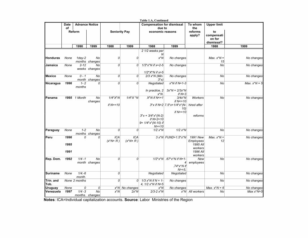
Table 1.A, Continued

Date of

Advance Notice Compensation for dismissal due to

To whom the

Upper limit

Reform Seniority Pay economic reasons reforms apply?

to compensati

on for dismissal?

1990 1999 1988 1999 1988 1999 1988 1999 2 1/2 weeks per

N

Honduras None 1day-2 months

No changes

0 0 x*N No changes Max. x*N = 15

No changes

Jamaica None 2-12 weeks

No changes

0 0 1/3*x*N if x=2-5 No changes No No changes

1/2*X*N if x>5 Mexico None 0 - 1

month No

changes0 0 2/3 x*N (Min.

3*x)No changes No No changes

Nicaragua 1996 1- 2 months

0 0 0 Negotiated x*N if N=1-3 No Max. x*N = 5

In practice, 2 x*N.

3x*N + 2/3x*N if N>3

Panama 1995 1 Month No changes

1/4*X*N 1/4*X *N X*N if N<=1 3/4x*N if N<=10

Workers No No changes

if N>=10 3*x if N=2 7.5*x+1/4*x*(N-10)

if N>=10

hired after

3*x + 3/4*x*(N-2) if N>2<10

reforms

9+ 1/4*x*(N-10) if N>=10

Paraguay None 1-2 months

No changes

0 0 1/2 x*N 1/2 x*N No No changes

Peru 1996 0 0 ICA (x*N+ R )

ICA (x*N+ R )

3 x*N FUND+1.5*x*N 1991 New Employees

Max. x*N = 12

No changes

1995 1995 All workers

1991 1996 All workers

Rep. Dom. 1992 1/4 -1 month

No changes

0 0 1/2*x*N .67*x*N if N=1-4

.74*x*N if N>=5,

New employees

No No changes

Suriname None 1/4.-6 month.

0 Negotiated Negotiated No No changes

Trin. and Tob.

None 2 months 0 0 1/3 x*N if N = 1-4, 1/2 x*N if N>5

No changes No No changes

Uruguay None 0 0 x*N No changes x*N No changes Max. x*N = 6 No changesVenezuela 1997 1/4 -3

months. No

changesx*N 2x*N 2/3-2 x*N x*N All workers No Max x*N=5

Notes: ICA=Individual capitalization accounts. Source: Labor Ministries of the Region

Appendix B1

Dynamic Demand Specifications

All of the papers on labor demand in this volume ignore the asymmetric nature of labor

demand. In this appendix, we explore the consequences of asymmetry on labor demand.

In order to specify labor demand functions in the presence of hiring and firing costs, it is

convenient to use a two period model. Such a model is implicit in Kugler (this volume). Let

f( ) denote output as a function of labor input . Let θ be a demand shock. We assume

that workers do not quit.

Labor hired in period 1 is 1. Labor employed in period 2 is 2 = 1 + ∆. ∆ is thus

the change in the stock of period 1 labor in period 2. The spot wage W is assumed to be

common in both periods, and is assumed to be exogenous to the firm. The cost of firing a

worker is C. Assume no discounting. Amount 1 is kept on in period 2 unless second period

demand shocks (θ) are sufficiently low. The firm maximizes

f( 1)−W 1 +E[θf( 1 +∆)−W ( 1 +∆)− C(Max(−∆, 0)]. (B-1)

We assume the support of θ is [0,∞) and that θ is an (absolutely continuous) random

variable. If θ ≥ 1 with probability 1, the firm in the second period wants ∆ ≥ 0. Intuitively,

labor productivity has increased.

The presence of second period firing costs inhibits hiring in the first period. Thus,

anticipating the possibility of an adverse shock in the second period, the firm hires less labor

than it would in the first period when labor productivity is unity. If we characterize the firm

1We thank Jagadeesh Sivadasan for helpful comments on this draft.

myopically as a period-by-period profit maximizer, the firm acts as if θ were less than one

in the first period. Letting θ be the value of the perceived first period productivity shock, if

θ > θ in period 2, then θf 0( 2) =W and 2 = [f0]−1

µW

θ

¶> 1.

If θ = θ, the firm stays put at 1 so that 1 = 2 and ∆ = 0. If productivity is below θ2,

the firm may still keep its workforce at 1 = 2 because it is costly to fire labor. We now

determine the lower bound on θ that gives rise to inaction. For a fixed 1, the condition

required for inaction (∆ = 0) is θf 0( 1) < W , so it pays in gross terms to get rid of a unit of

1 and θf 0( 1) > W − C, so it does not pay in net terms. Thus the inequalities in the zone

of inaction are determined by

W − C ≤ θf 0( 1) ≤W.

The critical value of the lower boundary θ∗ is

W − C

f 0( 1)= θ∗.

Holding 1 fixed, raising C lowers the threshold θ∗.

The first order condition for 1 is f 0( 1) −W + E(θf 0( 1 +∆) −W ) = 0, where ∆ = 0

if θ∗ ≤ θ ≤ θ, ∆ < 0 if θ < θ∗ and ∆ > 0 if θ > θ. From concavity, 1 is decreasing in cost

C. Intuitively, firms with high firing costs hold back on hiring 1. There is an option value,

in this case, of holding back on hiring 1 to avoid the cost of firing unwanted second period

labor. In order to characterize 1, we must first characterize ∆( 1).

2

Second Period (Conditional on 1) Demand Functions

Letting ∆− denote the decline in the stock, we obtain the first order condition for ∆− as

θf 0( 1 +∆−) =W − C

or

1 +∆− = (f 0)−1µW − C

θ

¶.

Take 1 as given. Observe that if 0 < θ < θ∗, ∆ < 0 Define ϕ ≡ f 0−1. Observe that ϕ < 0.

Then

1 +∆− = ϕ

µW − C

θ

¶.

Observe that at θ = θ∗, ∆− = 0. If θ > θ, θf 0( 1 +∆+) = W and ( 1 +∆+) = ϕ

µW

θ

¶. If

θ∗ < θ < θ, the firm operates at 1 and ∆ = 0. Define g(θ) as the density of θ which we

assume exists. Given 1, expected demand in period 2 (averaged over the θ states) is, for a

given firm,

E( 2 |W,C, 1) =

θ∗Z0

ϕ

µW − C

θ

¶g(θ)dθ + 1

θZθ∗

g(θ)dθ

+

∞Zθ

ϕ

µW

θ

¶g(θ)dθ.

3

Thus

∂E( 2 |W,C, 1)

∂W=

∂θ∗

∂Wϕ

µW − C

θ∗

¶g(θ∗)

+

θ∗Z0

1

θϕ0µW − C

θ∗

¶g(θ)dθ

+

∞Zθ

µ1

θ

¶ϕ0µW

θ

¶g(θ)dθ

+ 1

·∂θ

∂Wg(θ)− ∂θ∗

∂Wg(θ∗)

¸−µ

∂θ

∂W

¶ϕ

µW

θ

¶g¡θ¢,

∂E( 2 |W,C, 1)

∂C=

µ∂θ∗

∂C

¶ϕ

µW − C

θ∗

¶g(θ∗)−

θ∗Z0

1

θϕ0µW − C

θ

¶g(θ)dθ

+ 1

·∂θ

∂cg(θ)− ∂θ∗

∂cg(θ∗)

¸− ∂θ

∂cϕ

µW

θ

¶g¡θ¢.

Using ϕµW − C

θ∗

¶= 1 and ϕ

µW

θ

¶= 1

∂E( 2 |W,C, 1)

∂W=

θ∗Z0

1

θϕ0µW − C

θ

¶g(θ)dθ

+

∞Zθ

1

θϕ0µW

θ

¶g(θ)dθ

4

and hence

∂E( 2 |W,C, 1)

∂C= −

θ∗Z0

1

θϕ0µW

θ

¶g(θ)dθ.

If θ is iid across firms in period 2, and iid across time, then the average conditional (on

1) labor demand function is not a direct function of either W or W +Pr(0 < θ < θ∗)C. In

fact, the model predicts that

∂E( 2 |W,C, 1)

∂W+

∂E( 2 |W,C, 1)

∂C< 0

so that∂E( 2 |W,C, 1)

∂Wis larger in absolute value than

∂E( 2 |W,C, 1)

∂Calthough they are

of opposite signs.

This suggests that in empirical specifications of demands we should use C and W sep-

arately. Notice, however that OLS regressions of demand functions do not identify the

standard substitution terms used in static demand analysis.

One way to avoid problems with direct estimation of labor demand functions is to estimate

production functions. These can be used to derive the demand functions given fixed costs

without directly estimating demand functions with fixed costs.

5

First Period Demand Functions

These are obtained by substituting each state-contingent 2 = 1 +∆ demand function

into (B-1) and maximizing with respect to 1. As in the analysis of the second period demand

function, W + Pr(0 < θ < θ∗) C is not an appropriate marginal price in any state. Upon

substitution, we obtain total profits (as perceived in the first period) as

f( 1)−W 1 +

θ∗Z0

£θf( 1 +∆−(W,C, 1, θ))− (W − C)∆− −W 1

¤g(θ)dθ

+

θZθ∗

[θf( 1)−W 1] g(θ)dθ

+

∞Zθ

£θf( 1 +∆∗(W,C, 1)−W ( 1 +∆+)

¤g(θ)dθ.

Assuming an interior solution, and using the envelope theorem,

f 0( 1)−W +

θ∗Z0

[θf 0( 1 +∆−(W,C, 1, θ))−W ]g(θ)dθ +

θZθ∗

[θf 0( 1)−W ]g(θ)dθ = 0

so the first period demands obtained as the solution to this equation are functions of W

and C separately and not W + Pr(0 < θ ≤ θ∗)C. Observe, trivially that the 1 from this

equation is lower than the 1 when C = 0.

6

Appendix CA Framework for the Study of the Effects ofLabor Market Policies with Asymmetric Costs

and Entry and Exit

Alessandro Barbarino and James Heckman

1. The Simplest Framework

Consider an industry made up of Þrms producing a homogeneous good. TheseÞrms choose each period the number of employees to hire. There is no capi-tal. Each Þrm is hit each period by an idiosyncratic shock (iid across Þrms butcorrelated through time). The only element dictating the size of each Þrm is aMarkovian exogenous shock process. This shock approach is a very poor theoryof the Þrm. Still it allows us to derive the size distribution of Þrms in a dynamicsetting in equilibrium and allows us to introduce some Þring-costs policy analy-sis. Notice also that the notion of efficiency is again fully embodied by the currentshock the Þrm is exposed to: there is nothing structural which suggests what Þrmshould exit the industry because it has become inefficient.1

1.1. Firms

The model we will use can be described as a representative Þrm which is maximiz-ing proÞts in an intertemporal setting. The Þrm needs to choose the number ofemployees each period nt; this choice would be static without Þring-hiring costs:in their presence the problem is similar to the problem of investment choice in thecapital adjustment cost literature. In addition it can choose to exit the market

1An easy way out could be to introduce some exogenous heterogeneity.

1

forever. The exit decision is relevant since there are Þxed costs to be paid eachperiod to stay in the industry. If prospective revenues are not high enough theÞrm might decide to exit. With exit, also the entry decision needs to be mod-eled. Entry is determined by a zero future proÞts condition. For convenience, inthe simulation the horizon is assumed to be inÞnite. We proceed to describe thebuilding blocks of the model in subsequent points:

The Þrm has a production function with only one input: labor, denoted asnt. The production function is Cobb-Douglas. It depends also on a shock stwhich can be interpreted as a demand shock or a productivity shock:

Ft(nt, st) = stnat

The simplest shock process is a two state Markov chain. Here we adopt anAR(1) since it will be easier to bring this model to the data:

log st = c+ ρ log st−1 + εt

where εt ∼ N(0, σ2ε).We denote the long run mean of the process as m= c1−ρ .

Price of the consumption good is normalized to unity; Wage is allowed to adjust to set the model to equilibrium; Adjustment costs are assumed to be linear:

g(nt, nt−1) = max(0, nt−1 − nt)

Firing costs will be:

f(nt, nt−1) = fmax(0, nt−1 − nt)

Hiring costs will be:

h(nt, nt−1) = hmax(0, nt − nt−1)

In the simulation Þring costs f are set as a function of wage: f=ff*wage. Thesame is for hiring costs: h=hh*wage. ff and hh are two coefficients whichrepresent the policy. Varying the policy boils down to changing those twocoefficients.

2

Timing:

The representative Þrm faces the following timing:

1. Incumbent begins period t with (st−1, nt−1);

2. it looks at prospective future discounted proÞts and decides to exit [Xt = 1]or to stay [Xt = 0];

3. if it exits it gets -g(0, nt−1);

4. if it stays, it produces getting a period return of:

[stnat − wnt − cf − f max (0, nt−1 − nt)− hmax (0, nt − nt−1)]

The representative Þrm solves the sequential problem:

maxnt,Xt

E0

∞Xt=0

bt (1−Xt)πt −Xtg(nt, nt−1)

Xt =

½1 if exit0 if stay

all t.

s.t. nt ≥ 0 all t.

where b is the discount rate and πt proÞts at t. The Þrm is assumed tomaximize the discounted future stream of proÞts:

maxnt,Xt

E0

∞Xt=0

bt(1−Xt) [stnat − wnt − cf − f max (0, nt−1 − nt)− hmax (0, nt − nt−1)] +

+Xtf max (0, nt−1 − nt)

Xt =

½1 if exit0 if stay

all t.

s.t. nt ≥ 0 all t.

3

The problem above is mapped, as it is standard practice for simulations,into the Bellman equation:

V (n, s;w) = maxn0≥0

[sn0a − wn0 − cf − f max (0, n− n0)− hmax (0, n0 − n)] +

+bmax [EV (n0, s0;w),−f max (0, n0)] The Bellman above is used in Hopenhayn and Rogerson (1993). Given thetiming it would have been more natural to write:

V (n, s;w) = max−f max (0, n0) ,maxn0≥0

Es[sn0a−wn0−cf−f max (0, n− n0)−

−hmax (0, n0 − n) + bmaxEs0V (n0, s0;w)]but this is unnecessarily complicated and no different from the previous one.

Example 1. Assume that hh≡ 0 and ff≡ 0. Derive the optimal policy function:

n∗t+1 = gt+1(n∗t , st)

In this case the solution of the dynamic problem turns out to become very simple:it loses its dynamic aspect and the problem becomes a sequence of static problems.The FOC in this case becomes:

astna−1t = w =⇒ n∗t =

³astw

´ 11−a

or taking logs:

logn∗t =1

1− a (log a− logw + log st)which it implies that

log st = (1− a) log n∗t − log a+ logw

Now substitute log st = (1− a) log nt− log a+logw and log st = c+ρ log st−1+ εtinside the FOC for nt+1 to Þnd:

log n∗t+1 =1

1− a (log a− logw + c+ ρ [c + (1− a) logn∗t − log a+ logw] + εt−1)

4

=⇒ log n∗t+1 =½µ

1− ρ1− a

¶[log a− logw] + c

1− a¾+ ρ log n∗t +

1

1− aεt+1 (1)

We have derived the optimal policy in this simple case. We can see how the shockprocess enters into the optimal policy function (which will be the law of motion ofntimplied by the model). The relation obtained can be brought to the data witha simple time-series regression:

log nt+1 = α+ β log nt + 8t+1

Note that, as the theoretical persistence of the shock ρ increases in equation 1, thepersistence parameter on lagged labor increases as well in the same equation. Thisimplies that also bβ(≡ bρ) is expected to be higher when estimated from simulationdata. This should warn us that a high estimate of β on real industry data doesnot necessarily mean high Þring costs; it might mean simply high serial correlationin the error term. Notice that a serial correlated error term does not invalidateconsistency of bβ. For efficiency it is better to control for serial correlation in theerror term running GLS. In this case it is really GLS since the Ω is known:

Ω =σ+

(1− ρ2)

1 ρ · · · ρT−1

ρ 1 · · · · · ·· · · · · · · · · ρρT−1 · · · ρ 1

and the transformation matrix P=Ω−

12 :

P = Ω−12 =

1

σu

p1− ρ2 0 0 · · · 0−ρ 1 · · · 0 · · ·0 −ρ · · · · · · 0· · · · · · · · · 1 00 · · · 0 −ρ 1

so that the regression is run with dependent and independent variables trans-formed as follows:

y∗ =

p1− ρ2y1y2 − ρy1· · ·

yT − ρyT−1

X∗ =

p1− ρ2x1x2 − ρx1· · ·

xT − ρxT−1

the corresponding error terms 8∗ will be uncorrelated.

5

1.1.1. Aggregate Quantities Coming from the Problem of the Firm

In this subsection we deÞne the aggregate quantities which will be needed tosimulate the model.Aggregate Labor Demand:

LD (µ,M ;w∗) =Xs,n

N(n, s;w∗)µ(n, s;w∗,M) +Ms_grid(1,S)Xs=s_grid(1,1)

N(0, s;w∗)υ (s)

Aggregate Output:

Y (µ,M ;w∗) =Xs,n

[sN(n, s;w∗)a − cf ]µ(n, s) +Ms_grid(1,S)Xs=s_grid(1,1)

sN(0, s;w∗)aυ (s)

Aggregate Labor Taxes:2

R (µ,M ;w∗) =Xs,n

[1−X(n, s;w∗)]s_grid(1,S)Xs=s_grid(1,1)

fmax (N (n, s0;w∗) , n)P (s, s0)+

+X(n, s;w∗)fmax (0, n)Aggregate ProÞts:

Π (µ,M ;w∗) = Y (µ,M ;w∗)− w∗LD (µ,M ;w∗)−R (µ,M ;w∗)−Mce

1.2. Consumers

Consumers are modeled in a very simple fashion: there is a representative agentwho maximizes

maxU (C,N) = maxct,Nt

∞Xt=1

βt [u (ct)− ANt]

s.t. ct = wNt +Πt +Rt

where R are rebates from the Government to the consumers of the taxes collectedvia Þring costs. Π are proÞts from Þrms.

2There is a typo in Hopenhayn and Rogerson (1993). Their expression seems incorrect giventheir timing.

6

It is assumed that:

u (ct) = ln ct

The conditions for an optimum, using the BC into the utility are found:

maxNt

∞Xt=1

βt [ln (wNt +Πt +Rt)− ANt]

w

wNt +Πt +Rt− A = 0 =⇒ NS

t =1

A− Π+R

w

This setting is clearly very simple: it does not allow for search costs and un-employment insurance. The assumption that taxes collected from Þring costs aresimply rebated to the consumers via the Government is also too simple: it is thesimplest device to avoid that Þrms contract directly with workers to undo Þringprovisions.It is possible to derive aggregate labor supply as:

LSt = N∗t =

1

A− Π+R

w

1.3. A Solution Algorithm

The algorithm that we implement works in the following way:

1. Fix a wage w;

2. Iterate on the value function:

Vτ(n, s;w) = maxn0≥0

[sn0a − wn0 − cf − f max (0, n− n0)− hmax (0, n0 − n)] +

+bmax [EVτ−1(n0, s0;w),−f max (0, n0)]to obtain the optimal policies N(st−1,nt−1;w) and X(st−1,nt−1;w); τ is com-putation cycle number.

3. Compute w* that satisÞes the zero proÞts condition:

EυV (0, s0;w∗) = ce

7

where EυV (0, s0;w∗) is the expected value of entry. In the discrete approxi-mation of the simulation it is:X

s0V (0, s0;w∗)υ (s0) = ce

or:s_grid(S)Xs0=s_grid(1)

V (0, s0;w∗)υ (s0) = ce

Notice that the equilibrium wage so found does not depend on anything elsebut the previous step. Notice also that the previous step is not modiÞed bywhat follows. This means that the rest of the algorithm does not change thevalue for w* found. It was relatively easy to Þnd w*.

4. Now Þx a scale scalar (say M=1);

5. Find the mass of Þrms that will transit to the location (n,s) next periodwith the formula:

µ0τ(n0, s0;w∗,M) =

Xn,s s.t. N(n,s;w*)=nand X(n,s;w*)=0

µτ−1(n, s;w∗,M)P (s, s0)+

+υ(s0)M1(n0 = 0)

again, τ is computation cycle number.

6. Iterate on the previous equation to Þnd its Þxed point3:

µ∗ (n, s;M) = Tµ∗(n, s;M)

7. Now Þnd the M* which satisÞes the following labor market condition:

LD (µ∗ (M∗) ,M∗, w∗) = LS(Π(µ∗,M∗) +R(µ∗,M∗), w∗)

3The Þxed point of the operator:

Tµ =X

n,s s.t. N(n,s;w*)=nand X(n,s;w*)=0

µ(n, s;w∗,M)P (s, s0) + υ(s0)M1(n0 = 0)

8

It is quicker to Þnd the M* that satisÞes the following condition:

Uc (c(M∗), N(M∗))

UN(c(M∗), N(M∗))=1

w∗

where w∗is determined in step 3; the condition above can be written also as:

A

c=1

w∗→ c =

w∗

A

and imposing the equilibrium condition4 YM*=c it can be rewritten as:

YM∗ =w∗

A→M∗ =

w∗

AY

Y is computed as:

Y (µ,M ;w∗) =Xs,n

[sN(n, s;w∗)a − cf ]µ(n, s)+Ms_grid(1,S)Xs=s_grid(1,1)

sN(0, s;w∗)aυ (s)

1.4. Calibration of the Shock Process

In the simulations we adopt a 6-states Markov process. To map the AR(1) processinto the Markov process We simulate the AR(1) for 50000 periods with initialcondition long-run mean and we record realized values into bins. Then the relativefrequencies are used to construct the transition matrix P for the correspondingMarkov process. We denote the long run mean of the process as m= c

1−ρ . Thedistribution of shocks for new entrants is υ (s). It is chosen so that the distributionof Þrms by size matches the empirical one in the U.S.

1.5. The Rest of the Parameters

The following table sums up the parameters present in the model. The valuesare set to match microeconomics studies and they correspond to the values in thepaper Hopenhayn and Rogerson (1993).Firms:4Where Y is the aggregate product of the industry.

9

a Coefficient in the Cobb-Douglas 0.64ff Þring cost as a percentage of wage varyinghh hiring cost as a percentage of wage varyingb discount factor 0.8cf Þxed cost of staying in the industry 0.5ce Þxed cost of entry 0.2Consumers:A disutility of work parameter 0.5

1.6. Results

In this section we report the results of the simulations.

1.6.1. Policy functions

Two policy functions are considered into this model. One is the labor policyfunction N which maps a previous level of employment nt and a current shock stinto an employment decision nt+1: nt+1 = N(nt, st). As it is theoretically derivedin Caplin and Krishna (1986), the policy function is composed of a region ofinaction and two threshold levels beyond which the Þrm wants to Þre or hire. Thefollowing picture is the simulated policy given the values of the parameters above.

10

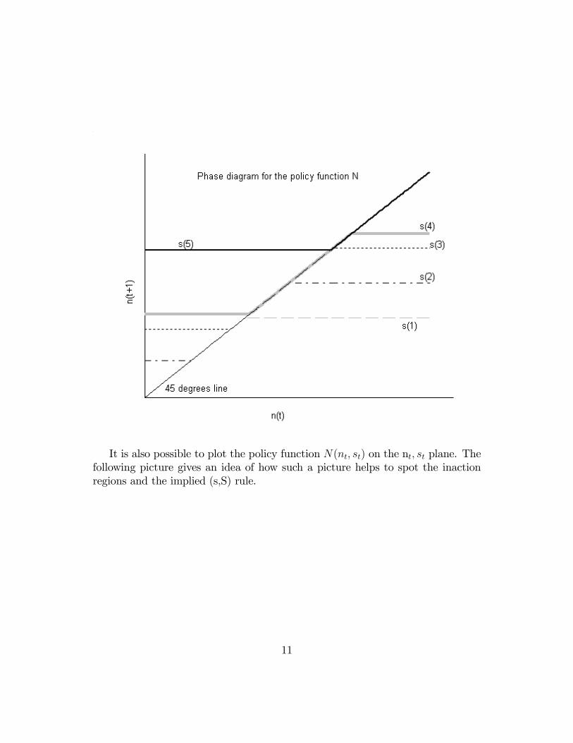
It is also possible to plot the policy function N(nt, st) on the nt, st plane. Thefollowing picture gives an idea of how such a picture helps to spot the inactionregions and the implied (s,S) rule.

11

Next is the simulation of a sample time path of employment and exit choices.Dots represent exit choices.

12

1.6.2. Results on the relationship between ρ and Þring costs

The following Þgure plots the optimal choices of a Þrm that faces no Þring costs.As it is clear and as derived in CASE 1 above, as the persistence of the relevantshock increases also nt becomes very persistent across periods.

The Þgure below reports results from simulations with Þring costs in place. ntis much more persistent.

13

The Þgure below makes clear that there is a clear-cut tradeoff between persis-tence in the underlying shock and level of hiring costs: couples (high Þring costsF, low persistence in idiosyncratic shock rs) may generate policy functions whichare as persistent as those generated by couples (low Þring costs F, high persistencers).

14

The next picture displays iso-curves: all couples that lie on those curves areassociated with the same estimated coefficient bρ in the regression:

log nt = b+ ρ log nt−1 + et

The regression above is estimated from the model where wage is normalizedto unity: this is why it does not include wages.

15

some iso-curves

0

0.2

0.4

0.6

0.8

1

1.2

0 0.2 0.4 0.6 0.8 1

f

r

iso-curve rhohat=0.95

iso-curve rhohat=0.85

iso-curve rhohat=0.79

References

[1] Hopenhayn, H. and R. Rogerson (1993). Job Turnover and Policy Evaluation:A General Equilibrium Analysis, The Journal of Political Economy, vol. 101.

[2] Caplin, A. and K. Krishna (1986). A Simple Dynamic Model of Unemploy-ment, working paper.

16