Laurence Freedman, PhD, MA Gertner Institute for … · measurement error on the estimation of usual intake distributions in the population. And the second concerns the impact of

The problem of measurement error when examining diet-health relationships

Laurence Freedman, PhD, MAGertner Institute for Epidemiology

Slide 1

Hello and welcome to the sixth webinar in the Measurement Error Webinar Series. I’m Sharon Kirkpatrick with the Risk Factor Monitoring and Methods Branch at the U.S. National Cancer Institute. We’re excited to kick off our sessions focused on examining diet and health relationships with today’s webinar.

Just before we get started, please note that the webinar is being recorded so that we can make it available on our Web site. All phone lines have been muted and will remain that way throughout the webinar. There will be a question and answer session following the presentation; you can use the Chat feature to submit a question.

A reminder: You can find the slides for today’s presentation on the Web site that has been set up for series participants. Other resources available include the glossary of key terms and notation, and the recordings of the preceding webinars.

Now it’s my pleasure to introduce the presenter for today’s webinar. Dr. Laurence Freedman is Director of the Biostatistics Unit at the Gertner Institute for Epidemiology, where he directs a research and consulting program in biostatistics and advises the government on public health policy. He has published extensively in the biostatistical literature, with particular emphases on cancer research and nutritional epidemiology. He has previously worked for the British Medical Research Council and the U.S. National Cancer Institute, where he was part of the team that developed the Women’s Health Initiative and the AARP Nutritional Cohort Study. Today Dr. Freedman will introduce the problem of measurement error when examining diet and health relationships. Welcome Dr. Freedman.

Thank you, Sharon.

Good morning, afternoon, or evening to everyone. For me it is late afternoon. Today, I will be describing the problems caused by dietary measurement error when we are trying to elucidate relationships between our diet and our health. (L. Freedman)

The problem of measurement error when examining diet-health relationships2

This series is dedicated to the memory of

Dr. Arthur Schatzkin

In recognition of his internationally renowned contributions to the field of nutrition epidemiology and his commitment to understanding measurement error

associated with dietary assessment.

Dedication

Slide 2

This series is dedicated to the memory of our dear colleague, Arthur Schatzkin.


Presenters and Collaborators

Sharon Kirkpatrick Series Organizer

Regan Bailey

Dennis Buckman

Raymond Carroll

Kevin Dodd

Laurence Freedman

Patricia Guenther

Victor Kipnis

Susan Krebs-Smith

Douglas Midthune

Amy Subar

Fran Thompson

Janet Tooze

Slide 3

And here is a list of the presenters and collaborators in this webinar series.


Two main areas of interest

Slide 4

For those who attended the first lecture, given by Sharon, you may remember that she mentioned two main themes to be covered in this series. One concerns the impact of measurement error on the estimation of usual intake distributions in the population. And the second concerns the impact of measurement error on the estimation of diet-health relationships.


Two main areas of interest

Slide 5

Well, the first theme is what you have mainly been hearing about in the first five lectures, and now in this sixth lecture, we are going to turn to the second theme regarding diet-health relationships.


Objectives

Learning objectives

Knowing the types and magnitudes of measurement error that occur in dietary data

Reviewing statistical models for evaluating diet-health relationships

Understanding the qualitative and quantitative impact of measurement error on studies of diet-health relationships

Slide 6

My aims today are: firstly, to inform you of the types of measurement error that we get in dietary data and their magnitude; secondly, to review some statistical models that we typically use to evaluate potential relationships between diet and health; and then to put these two parts together and explain the impact that dietary measurement error has on the results obtained from using these models.


INTRODUCTION

Slide 7

We'll start with a general introduction.


Introduction

Types of “analytic” studies

Animal experiments

Ecological studies

Cross-sectional studies

Case-control studies

Cohort studies

Randomized disease prevention trials

Red Estimated diet-health relationship impacted by dietary measurement error

Slide 8

There are a large variety of research designs that are used to investigate diet-health relationships, as seen in the list here, ranging from animal experiments down to randomized trials.

However, not all of these are impacted equally by dietary measurement error. The designs that are typed in red here are the ones that are most affected and, of these, I will be focusing on case-control studies and, particularly, cohort studies as the designs that are most commonly used to address such questions.


Introduction

The exposure (1)

In these studies we wish to relate:

The measure of intake thought to be most relevant is:

– usual intake, i.e., long-term average daily intake

Slide 9

Our main aim in these studies is to investigate the potential relationship between the intake of a dietary component, usually a nutrient or food, and a health outcome, very often the diagnosis of a specific disease, but sometimes also the level of a marker related to disease risk.

In investigating this question, although it is not always explicitly acknowledged, we are usually aiming to relate the usual intake of the dietary component to the health outcome, where by usual intake we mean a long-term average intake.


Introduction

The exposure (2)

In surveillance studies, “long-term” is often taken to be 1 or 2 years

In cohort and case-control studies, it is less-well defined but often may be thought of as covering several years

Slide 10

How long is long-term is also not often explicitly specified. In surveillance work, since population surveys are often conducted on an annual or biannual basis, the period is understood to be one or two years. In cohort and case-control studies it is less well-defined, but you can think of it as covering several years.


Introduction

The exposure (3)

Clearly, to measure an individual’s average intake over a long period is a challenging task

Fortunately, one does not need to measure usual intake exactly in order to make progress

Slide 11

Obviously, if measuring an individual's intake on a single day is no easy task, then measuring usual intake over several years is even harder. Fortunately, we don't have to measure it exactly to make progress. However, we have to accept that there will be some error in our measurement.


Introduction

Instruments (1)

–

–

–

–

–

–

Food Frequency Questionnaires

Main instrument for large cohort and case-control studies

Inexpensive to administer

Aims to measure long-term average intake

BUT

Inaccurate long-term recall

Cognitively difficult

Conversion to nutrient and food group intakes is difficult

Slide 12

The instrument for measuring an individual's usual intake that has been most widely used in cohort and case-control studies is the food frequency questionnaire. Its main advantages are of convenience and cost. It aims to capture usual intake but suffers from problems of inaccurate long-term recall and difficulties in cognition, and in the subsequent conversion of responses into nutrient and food group amounts.


Introduction

Instruments (2)

Slide 13

This slide illustrates some of the cognitive difficulties. It is taken from the food frequency questionnaire used in the Nurses' Health Study. Notice on this page for fruits intake the instruction on the left-hand side of the page. I will read it out. "Please try to average your seasonal use of foods over the entire year. For example, if a food such as cantaloupe is eaten four times a week during the approximate three months that it is in season, then the average use would be once per week." Needless to say, such averaging in one's head is hard, even for a statistician.


–

–

–

–

–

–

Introduction

Instruments (3)

24-hour recall

Main instrument for surveillance studies

Questions what the individual ate over the past 24 hrs

More accurate than FFQ (short-term recall only)

More detail makes conversion to nutrients easier

BUT

Very expensive to collect and code (up to now)

Does not target usual intake

Slide 14

An alternative to the food frequency questionnaire is the 24 hour recall. That instrument does carry some advantages over the food frequency questionnaire, but it does not target usual intake and also has been very expensive to collect and code.

Lately, a computerized version, the ASA24, has become available, and will soon be undergoing validation studies. It could be that a series of two to six computerized 24 hour recalls may in the future provide an alternative, or more likely, an added option to the food frequency questionnaire. In lecture 10 in the series, Doug Midthune will talk about combining food frequency questionnaires and 24 hour recalls. However, for today, we will assume that the study instrument is a food frequency questionnaire. Dietary intakes will, of course, be measured with error.


TYPES OF MEASUREMENT ERROR

Slide 15

In order to understand the impact of measurement error on study results, we first have to understand the different types of error that can arise.


Types of measurement error

Types of measurement error (1)

Additive systematic bias

– Systematic: the instrument introduces a bias that is common to all individuals

Ri = 0 + Ti

Ri denotes reported usual intake of individual i

Ti denotes true usual intake of individual i

(All reported values are different by the constant amount 0 from what they should be)

Slide 16

The simplest type of error is called additive systematic bias. This occurs when an instrument causes every measurement to be too large or too small by a constant additive amount. In this equation the amount of the error is denoted by the symbol beta subscript 0. The symbol R subscript i denotes the measurement on individual, i, and T subscript i is the true value.




5 10 15

Participant Number

1015

2025

3035

40

Usu

al in

take

TT

T T TT T T

T T T T T T T T T T T T

RR

R R RR R R

R R R R R R R R R R R R

Additive Systematic Bias: T=true value, R=reported value

20

Slide 17

This graph illustrates additive systematic bias. On the horizontal axis we have the identity number of a participant in the study. The T value denotes the participant's true usual intake and the R value, his or her reported intake. You can see that everyone underreports by the same amount. The quantity beta subscript 0 on the previous slide is therefore a negative quantity in this case.




Multiplicative and additive systematic bias

Ri = 0 + 1 Ti

(In addition to additive bias, the true value is scaled up or down by factor 1 )

Slide 18

The next step-up in complexity is that in addition to additive systematic bias we also have multiplicative systematic bias. The latter occurs when instead of reporting their true usual intake the participants all report a fixed multiple of that intake. Here, the multiplying factor is denoted by the symbol beta subscript 1, and is the same for all participants. If beta subscript 1 is less than 1 we get underreporting, and if it is greater than 1 we get overreporting. Putting the two sorts of systematic bias together gives the equation shown here.




5 10 15 20

Participant Number

1015

2025

3035

40

Usu

al In

take

TT

T T TT T T


RR

R R RR R R

R R R R R R R R R R R R

Multiplicative/Additive Systematic Bias: T=true, R=reported

Slide 19

This graph illustrates the situation described in the previous slide. In this case there is again underreporting but the amount of underreporting gets larger as the true usual intake increases. You can see that the underreporting is smaller here, at the lower end of the scale, than at the upper end. This occurs when beta subscript 1 is less than 1.


–



Person-specific (random) bias

Bias that occurs at the individual level - it is specific to an individual but can differ among individuals

Ri = 0 + 1 Ti + ui

(In addition to additive and multiplicative systematic bias, there is a bias ui that varies for each individual i)

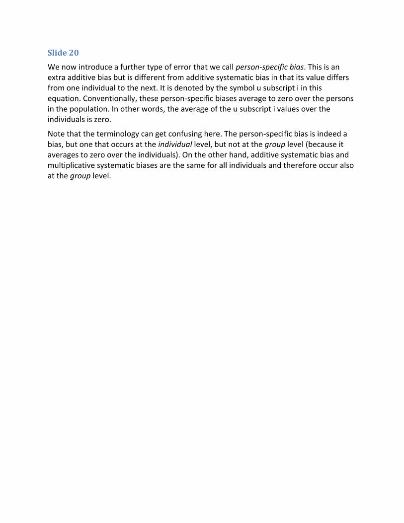
Slide 20

We now introduce a further type of error that we call person-specific bias. This is an extra additive bias but is different from additive systematic bias in that its value differs from one individual to the next. It is denoted by the symbol u subscript i in this equation. Conventionally, these person-specific biases average to zero over the persons in the population. In other words, the average of the u subscript i values over the individuals is zero.

Note that the terminology can get confusing here. The person-specific bias is indeed a bias, but one that occurs at the individual level, but not at the group level (because it averages to zero over the individuals). On the other hand, additive systematic bias and multiplicative systematic biases are the same for all individuals and therefore occur also at the group level.


–

–



Person-specific (random) bias

Ri = 0 + 1 Ti + ui

The subject-specific bias ui is a random term

Its magnitude is quantified by SD(ui ), its standard deviation

Slide 21

Because these person-specific biases vary from individual to individual, we think of them as random quantities. Since they are centered on zero, the magnitude of this type of bias is quantified by its standard deviation, which tells us how large it can get in either the positive or the negative direction.




5 10 15 20

Participant Number

1015

2025

3035

40

Usu

al In

take

TT

T T TT T T


RR

R RR

R

RR

RR

RR

R

R

R

R R RR

R

Multiplicative/Additive Group Bias Plus Person-Specific Bias

Slide 22

This graph illustrates the combined effect of the three types of error we have now described. Unlike the previous two graphs, the pattern in this one is haphazard, due to the random nature of the person-specific biases.




–

–

–

–

Within-person random error

Variation in reporting by an individual over a series of repeat reports

Rij = 0 + 1 Ti + ui + ij

The extra subscript j denotes the sequence number in a series of reports

The extra term ij is the within-person error that is on average zero

Its magnitude is quantified by SD(ij )

Slide 23

The final type of measurement error is called within-person random error, and represents the variation in reporting by an individual in a series of reports. This is related to the concept of the reproducibility of the report. To describe this sort of error mathematically, we introduce a new subscript, j, which denotes the sequence number in the series of reports. The term R subscript ij now represents the value given by person i on his or her jth report. The within-person error term epsilon subscript ij is the one that expresses the variation from one report to the next by the same person. None of the other terms on the right-hand side of the equation have a subscript j in them and so are fixed for that individual. The within-person random error terms average to zero over repeats within an individual and, as with person-specific bias, their magnitude is expressed by their standard deviation, denoted by SD of epsilon subscript ij.




5 10 15 20

Participant Number

1015

2025

3035

40

Usu

al In

take

TT

T T TT T T


RR

R

R R

R

R

R

R

R

R

R

R

R

RR

RR

RR

General Situation: systematic bias, person-specific bias, random error

Slide 24

And here is the last graph of this type, which shows a similar pattern to the previous one, except that there is now even more haphazardness because we have two independent random effects working in consort: person-specific bias and within-person random error. When we use food frequency questionnaires, or any dietary self-report, we encounter all four types of error working together.


EVALUATING THE MAGNITUDE OF ERROR

Slide 25

In order to get a handle on how much these errors impact on research results, we have to know how large they are, so we next turn to their magnitude.


Evaluating the magnitude of error

Evaluating the error (1)

How can we study the errors made in dietary reporting?

– Validation studies comparing reports with “reference” measures of dietary intake

Ideal properties of a reference instrument

i. Unbiased

ii. Errors uncorrelated to true intake

iii.Errors uncorrelated with self-report errors

Slide 26

Ideally, to measure the magnitude of errors we would like to compare reported usual intakes with their true values. However, we cannot measure these true values exactly.

The best we can do is to conduct validation studies in which we compare self-reported usual intakes with "reference" measures. The best kind of reference measure to use, short of the true value, is one that: first, is unbiased, meaning that if we repeated it many times and took an average, it would get very, very close to the individual's true value; second, has errors that are unrelated to the true usual intake; and, third, has errors that are unrelated to errors in the self-report instrument that we are validating—the food frequency questionnaire.




–

–

•

•

•

–

Do we have any ideal “reference” measures?

Direct observation (feeding studies)

“Recovery” biomarkers: based on recovery of specific biologic products that are directly related to intake and are not subject to substantial inter-individual differences in metabolism

Doubly labeled water for energy intake

24-hour urinary nitrogen for protein intake

24-hour urinary potassium for potassium intake

“Concentration” biomarkers (e.g., serum lipids) do not share these properties

Slide 27

The question is whether we have any such reference measures.

One possibility is where we directly observe what people eat, but this is usually only possible within the context of providing the participants with all their food requirements in a feeding study. The problem then is that the participants are not in a free-living environment and may not self-report their consumption in the usual way.

A second possibility is to use "recovery" biomarkers, based on recovery of specific biologic products that are directly related to intake and are not subject to substantial interindividual differences in metabolism. However, there are only three known examples of such biomarkers, as shown in this slide: Doubly labeled water for energy intake; 24 hour urinary nitrogen for protein intake; and 24 hour urinary potassium for potassium intake.

Other biomarkers, known as concentration biomarkers, do not enjoy the properties of a reference measure that you saw on the previous slide. They are useful in other ways but not for the validation of questionnaires. I will talk more about these other uses in lecture 11 of the series.




–

–

–

–

–

–

–

OPEN (Observing Protein and Energy Study)

261 men; 223 women

Adult volunteers residing in Maryland, USA

Completed:

24-hour recall x 2

Food frequency questionnaire x 2

24-hour urinary nitrogen x 2

24-hour urinary potassium x 2

Doubly-labeled water x 1 (in 25 persons x 2)

Slide 28

The earliest large validation study with recovery biomarkers was the OPEN study, whose features are shown in this slide. It included nearly 500 healthy adult volunteers who completed a 24 hour recall and a food frequency questionnaire and provided assessments using the three recovery biomarkers I just mentioned. Repeat measures of each were included.




Results from OPEN – Means

Sex Method Energy(kcal/d)

Protein(g/d)

Men

Marker 2842 105.5

FFQ 1961 74.7

24HR 2522 92.2

Marker 2273 77.5

Women FFQ 1524 57.2

24HR 1919 70.9

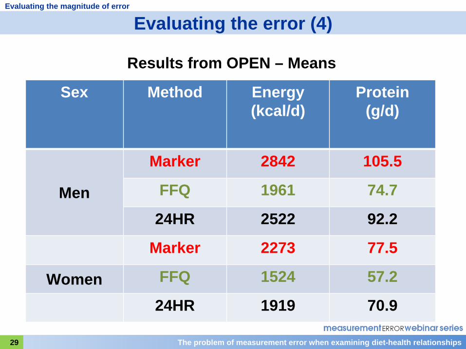
Slide 29

Here are some results from OPEN regarding bias in self-reporting at the group level.

You can see that both for energy and protein intake there is substantial underreporting using the food frequency questionnaire. For example, you can see that for energy intake in men, the mean report on the food frequency questionnaire was 1961 kcal compared to 2842 kcal obtained using the biomarker. There was also some underreporting, but not as much, using the 24-hour recall, as seen in the mean value of 2522 kcal, here. The amount of underreporting of both energy and protein is about 30 percent on the food frequency questionnaire and 10-15 percent on the 24 hour recall.



Evaluating the error? (5)

Results from OPEN – Protein Intake (after log transformation)

Sex Method Scaling Factor,

ß1

Person- Specific Bias

(SD)

Within- Person Error(SD)

MenFFQ 0.67 0.36 0.19

24HR 0.70 0.20 0.30

WomenFFQ 0.65 0.33 0.22

24HR 0.60 0.16 0.35

Slide 30

This slide shows the size of three measurement error parameters that we considered earlier. Those shown here are for protein intake.

The scaling factor is the factor that governs multiplicative systematic bias. The further it is from the value 1, the more severe is the bias. The slide shows that for protein intake the bias is quite marked for both the food frequency questionnaire and 24 hour recall.

The next column shows the standard deviation of the person-specific bias. The smaller this value, the better. You can see it is much larger for the food frequency questionnaire than for the 24 hour recall.

The final column shows that for within-person random error the pattern is reversed and is greater for the 24 hour recall than for the food frequency questionnaire. In other words, for the food frequency questionnaire the dominating error is person-specific bias, whereas for the 24 hour recall it is within-person random error. Part of the reason for the latter is no doubt due to daily variation in diet, since the 24 hour recall is a report of a single day.



Evaluating the error? (6)

Results from OPEN – Protein Density(after log transformation)

Sex Method Scaling Factor,

ß1

Person- Specific Bias

(SD)

Within- Person Error(SD)

MenFFQ 0.46 0.13 0.11

24HR 0.61 0.11 0.24

WomenFFQ 0.37 0.15 0.12

24HR 0.39 0.11 0.26

Slide 31

This slide shows the same measurement error parameters for protein density; that is, protein intake divided by energy intake. We call such a measure an energy-adjusted measure of protein intake, and I'll be talking more about energy adjustment later.

Notice that after this adjustment substantial improvements in measurement error parameters are seen, particularly for the food frequency questionnaire. The person-specific bias is greatly reduced by this adjustment, the standard deviation being reduced from about 0.35 to about 0.15, and there is also a considerable reduction in the within-person error, with a standard deviation of about half that seen for protein. Improvements are also seen with the 24 hour recall but are less dramatic.



Evaluating the error? (7)Summary of results of OPEN and other large validation studies (AMPM, NBS)

Serious under-reporting Energy: FFQ by 30% and 24HR by 10%

Food frequency questionnaire (FFQ) Large systematic error, large person-specific bias, small within- person random error

The biases and random error can be reduced by energy adjustment

24-hour recall (24HR) Smaller systematic error, large within-person random error, smaller person-specific bias

The within-person random error of the 24HR is largely day-to-day variation and can be reduced by using several repeats

Slide 32

So here is a summary of the results from the OPEN study.


MODELS FOR ESTIMATING DISEASE RISK

Slide 33

Our ultimate aim in this lecture is to describe the impact of dietary measurement error on the results of research evaluating potential links between diet and health. A further necessary step before we do that is to review statistical models used in nutritional epidemiology for estimating disease risk.


Models for estimating disease risk

Estimating disease risk (1)

Before we study the impact of measurement error on studying diet-health relationships, we need to review measures and statistical models for disease risk

The two main measures of disease risk are:

–

–

Relative risk

Odds ratio

Slide 34

The two main measures of disease risk are the relative risk and the odds ratio.




When comparing two groups, exposed and unexposed:

Prob (disease in exposed)Relative risk =Prob (disease in unexposed)

Prob (disease)Odds (disease) = 1 - Prob(disease)

Odds (disease in exposed)Odds ratio = Odds (disease in unexposed)

Slide 35

When comparing two groups, one exposed to a given risk factor and one unexposed, the relative risk of disease associated with the exposure is the probability of developing the disease in the exposed group divided by the probability in the unexposed group.

Sometimes it is more convenient to use the odds of disease rather than the probability of disease. The odds is a measure that is commonly used in betting. The odds of disease is defined as the ratio of the probability of developing disease to the probability of not developing disease.

Then, the odds ratio associated with exposure is the odds of disease in the exposed group divided by the odds of disease in the unexposed group.

For rare diseases, the relative risk and the odds ratio are almost equal to each other, simply because the odds is almost equal to the probability of disease when the disease is rare.

Because in epidemiology we usually estimate relative risks and odds ratios via regression models, we now need to consider such models.




Elements of a nutrition regression model

1. A health outcome variable (Y)

2. A set of explanatory variables, (T1 ,T2 , Z1 …,Zp ) The T–variables are dietary exposures, and the Z-variables are other exposures, confounders, effect modifiers or intermediate variables

3. An equation linking the outcome to the explanatory variables

Slide 36

The elements of a regression model in nutritional epidemiology are: first, a health outcome variable, denoted by the symbol Y, which is often a binary variable indicating the presence or absence of disease; second, a set of explanatory variables that are dietary variables denoted by T subscript 1, T subscript 2, etc.; and other variables denoted by Z with a subscript. These Z-variables could be other nondietary exposures or confounders or effect modifiers or mediators.

Note that we use T for the dietary exposures to link with our earlier use of this symbol. They represent the true usual intakes of various dietary components.

The third element is an equation that links the health outcome to the explanatory variables—we call this the regression equation.




For example, logistic regression:

0 T1 1 T2 2 Z1 1 Zp plog{Odds(Y = 1)} = + T + T + Z +... + Z

Where: Y is a binary variable; Y=1 denotes disease (“case”) Y=0 denotes no disease (“healthy”)

's are the regression parameters and represent log odds ratios

Each

represents the increase in the log odds of

disease associated with increasing the corresponding variable by 1 unit while keeping the other variables fixed.

Slide 37

As an example, here is a logistic regression model that relates the odds of disease to dietary intakes and other explanatory variables. The Y is a binary variable indicating presence of disease when Y=1, or absence of disease when Y=0. It has been found very convenient to express disease risk (on the left-hand side of the equation) by the logarithm of the odds. In that case, the alpha-terms on the right-hand side, which are known as the regression coefficients, actually represent the logarithms of odds ratios. In fact, each alpha represents the increase in the log odds of disease associated with increasing its corresponding variable by 1 unit, while keeping the other variables fixed.




Estimating an odds ratio: binary exposure Israeli National Ovarian Cancer Case-Control Study

Oral Contraceptive use (0=<6m use, 1=6m+ use) 889 cases; 1747 controls

0 1{Odds(Y = 1)}log = + OC

Output from logistic regression program Coefficients:

Value Std. Error p value (Intercept) -0.65 0.046 <0.00010

ocon1 -0.13 0.100 0.19

Odds ratio estimate for OC = exp(1 ) = exp(-0.13) = 0.87

Slide 38

Here is a non-nutritional example of using logistic regression to estimate an odds ratio. The data are based on those from a study of risk factors for ovarian cancer conducted in Israel in the 1990s. The exposure of interest here is the use of oral contraceptives, which has been dichotomized as less than or more than six months of use. You can see that in the second line of the table in bold, the estimated coefficient for oral contraceptive use is -0.13. This is the estimated log odds ratio. To find the odds ratio we have only to take the exponent, which is equal to 0.87, a value less than 1, suggesting possible protection from the disease.



Estimating disease risk (6)Estimating an odds ratio: continuous exposure

Animal Fat intake (kcal/d) from a FFQ

0 1log{Odds(Y = 1)} = + afatcal

Output from logistic regression program Value Std. Error p value

(Intercept) -1.18 0.10 <0.0001 afatcal 0.0017 0.00030 <0.0001

Odds ratio estimate for increase in animal fat intake of 1kcal/d = exp(1 ) = exp(0.0017) = 1.0017

Odds ratio estimate for increase in animal fat of 100kcal/d = exp(1001 ) = exp(1000.0017) = 1.18

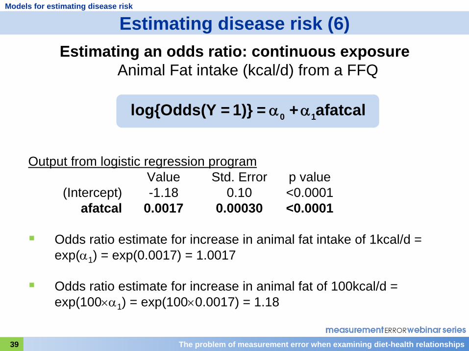
Slide 39

Here, now, is a nutritional example from the same study looking at the association of disease with intake of calories of animal fat reported on a food frequency questionnaire.

The estimated regression coefficient for animal fat intake of 0.0017 is very small, but highly statistically significant.

The odds ratio is again obtained by taking the exponent of the coefficient, and equals 1.0017, but this very small increase in risk is associated with a very small increase in animal fat intake, only 1 kcal. It would be more realistic to consider an increase of 50kcal or 100kcal.

The last line in the slide shows the calculation of the odds ratio for an increase of 100 kcal in animal fat intake, leading to an estimated odds ratio of 1.18.




Energy adjustment

–

Practical question:

A study has been conducted with a FFQ as the main dietary instrument

When evaluating an association between a FFQ-reported nutrient intake and the health outcome should one adjust for FFQ-reported total energy?

Slide 40

In the previous slide you saw a model with a single nutrient as the explanatory variable. An important issue in nutritional epidemiology concerns the question of whether to adjust for energy intake. If a food frequency questionnaire has been used for the study, the practical question becomes: If you want to study an association between a given FFQ-reported nutrient and a health outcome, should you adjust for FFQ-reported energy?




Possible reasons for energy adjustment (see Willett, Howe and Kushi, 1997)

Energy is a confounder

The energy-adjusted relative risk is more relevant to public health interests

The adjustment increases the precision of the relative risk estimate

Slide 41

In a paper written in 1997, Willet, Howe, and Kushi argued that one should adjust for energy intake. They advanced several reasons, but the one that seems most persuasive is that the energy adjustment increases the precision of the relative risk estimate. This is very closely connected to the results of the OPEN study, where we saw that energy adjustment appears to improve the measurement error profile of the food frequency questionnaire.




Energy adjustment models

There are several different methods for energy adjustment – we will look at two:

i. Standard model

ii. Density model

Slide 42

There are several ways to perform energy adjustment. We will look at two, one known as the standard model; the other, as the density model.





Standard model: Add total energy intake as a second explanatory variable, for example:

0 1 2log{Odds(Y = 1)} = + afatcal + energy

Meaning of the coefficient 1 changes: The log odds ratio associated with increasing animal fat

intake by 1 kcal while keeping total energy intake fixed

which means: The log odds ratio associated with substituting 1 kcal of animal fat for 1 kcal of other nutrients

Slide 43

In the standard model, we simply include FFQ-reported total energy intake as second explanatory variable, as shown in the regression equation here.

When we do this, it is important to realize that we change the meaning of the coefficient for animal fat intake. It is now the log odds ratio associated with increasing animal fat by 1 kcal while at the same time keeping total energy fixed. The only way we can increase animal fat intake by 1 kcal while keeping total energy intake fixed is by substituting the animal fat for 1 kcal of other nutrients. So the association is now with the substitution of animal fat for something else in the diet rather than with the addition of further calories of animal fat to the diet.




Energy adjustment: Standard model

0 1 2log{Odds(Y = 1)} = + afatcal + energy

Value Std. Error p value (Intercept) -1.39 0.13 <0.0001

afatcal 0.00093 0.00042 0.027 energy 0.00025 0.000098 0.009

Odds ratio for 100kcal increase = exp(0.00093 x 100) = 1.10

Remember that this association is with substituting 100kcal of animal fat for 100kcal of other food sources

Slide 44

Here is an example of using the standard model in the Israeli Ovarian Cancer Study.

Notice that the coefficient of the animal fat variable is reduced after inclusion of the total energy variable to about half of its previous value, 0.0017, and while the association is still statistically significant, the level of significance is less strong, 0.027. As before, it is possible to estimate an odds ratio associated with increasing animal fat by 100 kcal, but one needs to remember that this is an association with substituting that amount of animal fat for other nutrients.





Density model: Nutrient density = 100 x (nutrient intake in kcal / total energy intake in kcal)%

Express the nutrient as a nutrient density and add total energy intake as a second explanatory variable.

For example:

0 1 2log{Odds(Y = 1)} = + afatdens + energy

Meaning of the coefficient 1 : The log odds ratio associated with increasing animal fat density by 1% while keeping total energy intake fixed

Slide 45

A second way of performing energy adjustment is through the density model. A nutrient density is the percentage of total energy intake provided by that nutrient. In the density model, we express the nutrient intake of interest as a nutrient density and we also add total energy, a second explanatory variable, as shown in the regression equation here. Once again, we need to bear in mind that the coefficient of the nutrient density is a log odds ratio associated with a change in the composition of the diet, not in the total amount consumed.




Energy adjustment: Density model

0 1 2log{Odds(Y = 1)} = + afatdens + energy

Value Std. Error p value (Intercept) -1.66 0.20 <0.0001 afatdens 0.01560 0.00760 0.041

energy 0.00041 0.00007 <0.0001

Odds ratio for 5% increase = exp(0.0156 x 5) = 1.08

Remember that this association is with increasing animal fat density by 5% while keeping energy intake fixed

Slide 46

And here is an example of using the density model in the Israeli Ovarian Cancer study.

Notice that the level of significance of the coefficient for animal fat density, 0.041, is similar to that of the animal fat intake variable in the standard model. It is usually the case that the standard and density models yield similar levels of significance for the nutrient of interest.


QUALITATIVE IMPACT OF MEASUREMENT ERROR

Slide 47

Of course, there is a whole lot more one could say about the use of regression models in nutritional epidemiology, but I hope that what we have just covered will be sufficient for us now to address the question of the impact of dietary measurement error on the estimation of odds ratios or relative risks. In this next section I'll talk about the qualitative impact, and then later we'll consider its quantitative impact.


Qualitative impact

Qualitative impact of error (1)

Additive systematic bias

Suppose we have an instrument with additive systematic bias but no subject-specific bias and no random error.

Ri = 0 + Ti

Then: a. Log odds ratio estimates are unchangedb. Scatter about the regression line is unchangedc. Significance tests are unaffectedd. Study power is unaffected

Additive systematic bias is not a problem for detecting a relationship! But translation to public health message is affected

Slide 48

Before I talk about impact of measurement error on disease risk estimates, I have to explain an important assumption that I am going to make throughout the rest of the lecture. I will assume that the measurement error is the same for those with and those without disease. We refer to such error as nondifferential measurement error. This assumption is usually a very reasonable one for cohort studies where the dietary intake is reported usually many years before any disease is diagnosed. However, it is sometimes questionable in case-control studies where dietary reporting may be affected by disease status. For this lecture I am assuming that measurement error is nondifferential.

So, how do the different types of measurement error that we talked about earlier impact disease risk estimates? We'll start with additive systematic bias, and this slide reminds you what that is. This type of error actually has no impact on estimation of odds ratios or relative risks. The log odds ratio estimates are unchanged. The scatter about the regression line is unchanged. Significance tests are unaffected, as is statistical power of the study. This means that additive systematic bias is not a problem for detecting diet-health relationships, although it's important to remember that the translation of research results into public health recommendations would be affected. I'll explain that last remark in a bit more detail very shortly.


Qualitative impact


10 15 20 25 30 35 40

Fat Intake (g/d)

-4.2

-4.0

-3.8

-3.6

Log

odds

of d

isea

se

T T

T TT

TT

T TTT

TTT

TTT T

T

T

R R

R RR

RR

R RRR

RRR

RRR R

R

R

Effect of additive group bias on regression

Slide 49

In this slide I have tried to give you an intuition of why there is no impact on odds ratio estimates. The vertical axis of the graph represents disease risk on the log odds scale and the horizontal axis, usual dietary intake. The odds ratio is here represented by the slope of the straight line. Reported values, R, are displaced from the true values, T, along the x-axis by a constant amount. The slope through the R’s is therefore exactly the same as the slope though the T’s. Also, the scatter about the lines is the same for both the R’s and the T’s, indicating that the same statistical power for detecting an association will hold.

This graph also illustrates the point about the public health message. Suppose you wanted to achieve a log odds of disease of -4.0 or less in your population. Then according to reported intake values you would recommend a diet of 20 g/d of fat or less, whereas in truth eating 25 g/d or less would achieve the goal. It would therefore be necessary to adjust the public health message and correct for the additive systematic bias.


–

– – –

Qualitative impact


Additive and multiplicative systematic bias

Suppose we have an instrument with additive and multiplicative systematic bias but no person-specific bias and no random error

Ri = 0 + 1 Ti

Then: Log odds ratio estimates are scaled by 1/1Scatter about the regression line is unchangedSignificance tests are unaffectedStudy power is unaffected

Systematic bias is not the major problem for detecting a relationship!

Slide 50

When we have, in addition, multiplicative systematic bias, the picture changes slightly. Now the log odds ratio estimates become biased and are scaled by the factor 1 divided by beta subscript 1. Remember that the results of the OPEN study showed that, generally, beta subscript 1 is less than 1, so the log odds ratio estimates actually increase as a result of this multiplicative systematic bias. However, significance tests and statistical power to detect an association are not affected by the multiplicative bias. Because of this, and in view of what I will show you very soon, we have to conclude that systematic bias is not the major problem in detecting associations of diet with health outcomes.


Qualitative impact


10 15 20 25 30 35 40

Fat Intake (g/d)

-4.2

-4.0

-3.8

-3.6

Log

odds

of d

isea

se

T T

T TT

TT

T TTT

TTT

TTT T

T

T

R R

R RR

RR

R RRR

RRR

RRRR

R

R

Effect of additive and multiplicative group bias on regression

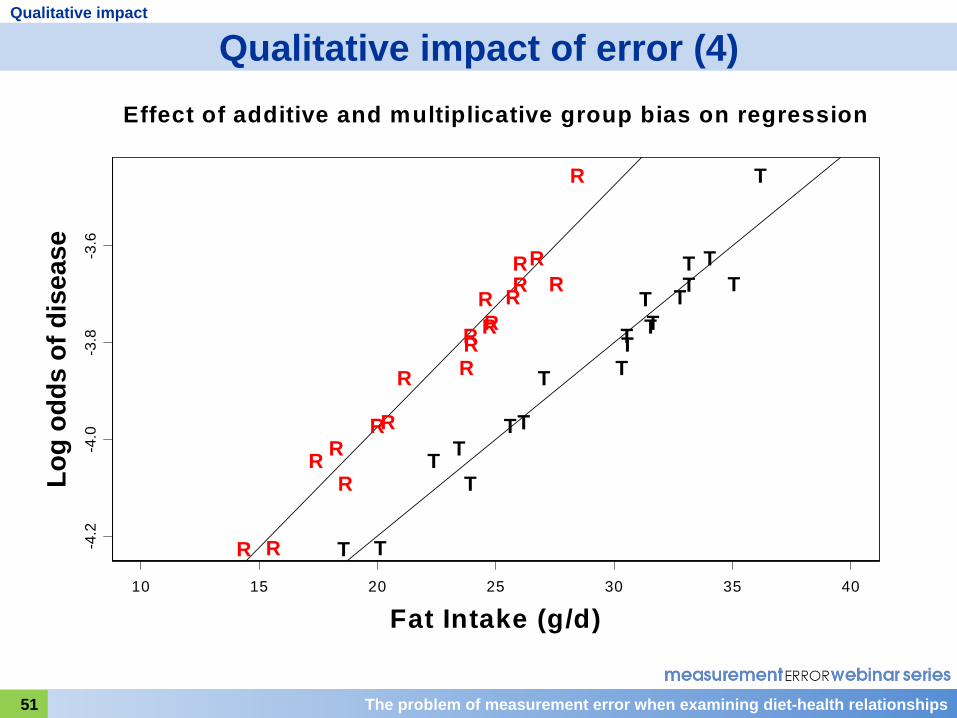
Slide 51

This slide shows the increase in slope resulting from multiplicative systematic bias that I just mentioned. But you can also see that the scatter about the regression lines through the R's is not increased and, therefore, statistical power is unaffected.


Qualitative impact


Person-specific bias and within-person random error

Suppose we have an instrument with systematic bias and also person-specific bias and within-person random error

Rij = 0 + 1 Ti + ui + ij

Then: a) Log odds ratio estimates are factored down

(attenuated)b) Scatter about the regression line is increasedc) Significance tests are less powerful but still validd) Study power is decreased

Person-specific bias and within-person random error are a major problem for detecting a relationship!

Slide 52

We now consider what happens if, as in the case of dietary self-reporting, you have systematic bias, person-specific bias, and within-person random error. The impact is, firstly, that log odds ratios become factored downwards; that is, towards the null value. We call this attenuation. Note that this occurs even though the multiplicative systematic bias tends to increase the log odds ratio. What happens is that the person-specific bias and within-person error both decrease the log odds ratio and, together, they overcome and dominate the effect of the multiplicative bias. In addition, the scatter about the regression line now increases, and although significance tests are still valid, they are less powerful. Because of the person-specific bias and within-person error, we lose power to detect the association. Thus, the random errors that are person-specific bias and within-person error are a major problem for detecting a diet-health relationship.


Qualitative impact


10 15 20 25 30 35 40

Fat Intake (g/d)

-4.2

-4.0

-3.8

-3.6

Log

odds

of d

isea

se

T T

T TT

TT

T TTT

TTT

TTT T

T

T

R R

R RR

R R

R RR R

RRR

R RRR

R

R

Effect of person-specific bias and within-person random error on regression

Slide 53

This slide shows the attenuation of the slope caused by the random errors, and you can also see the much greater scatter of points about the line that signifies the loss of power.


Qualitative impact


Summary

When a single dietary exposure measured with error is included in a disease outcome regression model:

Then: a) Log odds ratio estimates are factored down (attenuated)b) Study power is decreasedc) Significance tests are less powerful but still valid

These conclusions seems to hold also for several dietary exposures entered together in the same model (e.g., energy-adjustment models) – see later details

We now quantify the seriousness of these problems

Slide 54

So here is a summary of qualitative impact of dietary measurement error on results of research exploring diet-health associations. Note, first, that so far we have talking about the effects of measurement error when a single dietary intake measured with nondifferential error is entered as an explanatory variable into a regression model. In that case, log odds ratio estimates are attenuated, and although significance tests are still valid, they are less powerful. It seems, on the best evidence we have to date, that these same conclusions hold in the case where several dietary intakes all measured with error are entered into the regression model. I'll enlarge on that issue towards the end of the lecture.


QUANTITATIVE IMPACT OF MEASUREMENT ERROR: UNIVARIATE MODELS

Slide 55

We are now going to consider the quantitative impact for simple models where there is a single dietary intake as the explanatory variable.


Quantitative impact: univariate models

Quantitative impact of error (1)

We will now quantify the extent of the two main problems:

a) Log odds ratio estimates are attenuated

b) Study power is decreased

Slide 56

As we have just learned, the two main problems caused by dietary measurement error are the attenuation of odds ratio estimates and the decrease of study power. We will now see the size of these effects.




Log odds ratio attenuation for a single continuous dietary intake variable

–

–

Assume we have systematic error, subject-specific bias and random error.

Expected log odds ratio estimate = true value,

where

= attenuation factor = slope of regression of T (truth) on R (report)

is nearly always <1 and usually a lot less!

When the log odds ratio is attenuated, the odds ratio moves towards 1.0

Slide 57

Using statistical theory, it's possible to show that, under the type of measurement error in our instrument that we have been considering, the log odds ratio estimate that we expect to obtain is a factor lambda times the true value. For dietary data this factor lambda is nearly always less than 1. It has therefore become known as the attenuation factor (although some people call it the regression dilution ratio). The closer it is to zero, the worse the attenuation and, unfortunately, it is often a lot less than 1. Naturally, because the log odds ratio estimate is attenuated towards zero, the odds ratio estimate is attenuated towards 1.

It turns out that lambda is actually the slope of the regression of true usual intake, T, on reported intake, R. This is a very useful fact because it gives us a way of estimating the attenuation factor from validation studies such as OPEN, and we do this by regressing the recovery biomarker on the self-reported intake and estimating the slope.




Log odds ratio attenuation for a single continuous dietary intake

–

OPEN: Attenuation Factors for FFQ and 24HR (Men)

(Obtained by regressing recovery biomarker on self-report)

FFQ 24HR

Energy 0.08 0.18

Protein 0.16 0.20

Protein Density 0.40 0.23

Slide 58

This slide shows the estimates of the attenuation factors for men, obtained from the OPEN study. You can see that for the food frequency questionnaire, the estimates for energy and protein are extremely low, but that the attenuation factor for protein density is considerably higher. The situation is not much better for a single 24 hour recall, and in this case, energy adjustment does not improve matters greatly.




Implications of these results

–

–

–

Suppose the attenuation factor is 0.16 (as for protein)

Suppose the true odds ratio between the 90th and 10th percentiles of true intake is 2.5

(i.e., substantial)

log OR = log(2.5) = 0.92

Expected estimated log OR = 0.92 x 0.16 = 0.147

Expected estimated OR = exp(0.147) = 1.16

Slide 59

The implications of such low attenuation factors can be seen in this slide. Suppose that, as seen for protein in the previous slide, the attenuation factor is 0.16. Suppose, now, that the true odds ratio is 2.5. The corresponding log odds ratio is 0.92. The measurement error causes this log odds ratio to be estimated on average as 0.92 times 0.16, which is 0.147, and this translates into an odds ratio of 1.16.




Implications of these results (cont’d)

Almost impossible to detect an OR of 1.16 in a case- control or cohort study

Reasons:

a) Enormous sample sizes required to obtain statistical significance (see later)

b) Cannot eliminate all confounding

The limit of detection for an OR is probably around 1.25

Slide 60

Such attenuation causes serious problems in nutritional epidemiology. It is almost impossible to detect an odds ratio of 1.16 in an observational study. Firstly, one requires enormous sample sizes to obtain statistical significance, and even if such significance is obtained one cannot rule out the possibility that the result is due to unmeasured confounders. Because of potential confounding, most epidemiologists consider that the limit of reliable detection of an odds ratio in observational studies is around 1.25, if not higher.




Implications of these results (cont’d)

–

–

–

Fortunately, after energy adjustment, attenuation factors with an FFQ are larger (e.g., 0.40 for protein density)

Suppose the true odds ratio between the 90th and 10th percentiles is 2.5 (i.e., substantial)

log OR = log(2.5) = 0.92

Expected estimated log OR = 0.92 x 0.40 = 0.368

Expected estimated OR = exp(0.368) = 1.44

Such an odds ratio is more possible to detect, although still difficult!

Slide 61

The picture is not totally bleak, since after energy adjustment for the food frequency questionnaire, the attenuation factor is increased. For protein density in a previous slide, it was 0.40. Going through the same calculation as previously, we see that a true odds ratio of 2.5 is estimated on average as 1.44, which is more possible to detect, although still hard.




Log odds ratio attenuation for a single categorized dietary intake

Assume we categorize our intake into quantiles (e.g., tertiles, quartiles or quintiles)

The log odds ratio is still attenuated but by a different amount:

Expected log odds ratio estimate =

true value,

where = correlation between R (report) and T (truth)

In other words, for analysis by quantiles, log odds ratios are attenuated by , instead of

Slide 62

Up to now, all the statistical analyses we have considered have been conducted on dietary intakes expressed as continuous variables. It is quite common practice to categorize dietary intakes into quantiles, such as tertiles, quartiles, or quintiles, and to estimate the odds ratio of persons in the highest quantile to those in the lowest. Such an odds ratio is also attenuated, but now the attenuation is governed by a different multiplicative factor, denoted by rho, which is the correlation between the reported intake and the true intake.




Log odds ratio attenuation for a single categorized dietary intake

OPEN: Correlations with True Usual Intake for FFQ and 24HR (Men)

FFQ 24HR

Energy 0.20 0.34

Protein 0.32 0.38


Slide 63

This slide shows the values of this correlation coefficient estimated from the OPEN study. Once again, you see low values. For the FFQ, the value increases after energy adjustment—that is, for protein density—to values similar to those seen previously for the attenuation factor.




Log odds ratio attenuation for categorized variables

Implications of these results are similar to those stated earlier

After energy adjustment, the estimated log odds ratios will be greatly attenuated by a factor of about 0.4 for protein density

Slide 64

So the implications for analysis with categorized variables are very similar to those for continuous variables.




Decrease in study power

Assume we have systematic bias, subject-specific bias and within-person random error

Effective sample size = Actual sample size x 2

Where: = correlation of R (report) with T (truth)

Slide 65

The second problem caused by measurement error is the reduction of statistical power to detect a diet-health association. Here also, we can quantify the effect using statistical theory. When we use a self-report instrument, R, that has correlation coefficient rho with the true usual intake, T, then we effectively reduce our effective sample size by a multiplicative factor equal to rho superscript 2. In other words, if our study has n participants, it has the same power as a study with n times rho superscript 2 participants who report their exact value of usual intake, T.





OPEN: Correlations with ‘truth’ for FFQ and 24HR (Men)

FFQ 24HR Energy 0.20 0.34Protein 0.32 0.38


Example: Protein Density FFQ: Effective sample size = 0.432 x actual sample size

= 0.18 x actual sample size

We effectively lose 82% of our sample size!

Slide 66

Here is the table of correlation coefficients between self-report and true usual intake, estimated from the OPEN data, which you saw a few minutes ago. Taking the example of protein density for the food frequency questionnaire, you can see that use of this instrument leads to an effective sample of 0.43 squared, or 0.18 times the actual sample size. In other words, use of this instrument, instead of obtaining an exact measure of intake (if that were possible) causes us to lose effectively 82 percent of our sample.





Suppose that we had calculated a sample size of 50,000 for a cohort study that would give 90% power for detecting an association the 5% significance level, assuming that we could measure dietary intake exactly

Then, because of the measurement error we would need 50,000/2 = 50,000/0.4322 = 270,000 to preserve the power of 90%

Slide 67

Another way of looking at this problem is to suppose that we had calculated that we needed a sample size of 50,000 for a cohort study investigating protein density to obtain 90 percent power for detecting an association with disease at the 5 percent level, assuming we could measure dietary intake exactly. Then, because of measurement error, we would actually need 50,000 divided by rho-squared; that is, about 270,000 individuals. The measurement error causes a more than fivefold increase in sample size requirements.


–

–




If we proceeded with the study with sample size 50,000 then the statistical power would be decreased by measurement error from 90% to 28%

The formula is given by:

Power = -1(3.24-1.96)

Where the symbol -1 denotes the inverse of the standard normal cumulative distribution function

Slide 68

And if we had forgotten to factor in the measurement error in our sample size calculations and we opted for a sample size of 50,000, then instead of obtaining 90 percent power to detect the association, we would have a power of only 28 percent. In other words, we would have a rather small chance of detecting the association. For those interested in performing such calculations, the formula is provided here.


QUANTITATIVE IMPACT OF MEASUREMENT ERROR: MODELS WITH MULTIVARIATE EXPOSURE

Slide 69

In the previous section we were considering the simple situation where there is only one dietary variable in the model. However, as we emphasized earlier, it is often recommended to include at least two dietary variables in the model—the nutrient of interest and total energy intake. So in this last section we will consider in more detail if the previous conclusions change when there is more than one dietary variable in the model.


Quantitative impact: multivariate models

Quantitative impact: multivariate exposures (1)

Two or more dietary variables in the disease regression model

Typical example: Standard energy-adjustment model log{Odds(Y=1)} = 0 + 1 afatcal + 2 energy

The effects of measurement error in these models is in theory less straightforward:

i. Estimated log odds may be biased but not attenuated (i.e., inflated)

ii. Statistical tests may not be valid

Slide 70

Consider a standard model that is one with both a nutrient—animal fat, say—and also energy, as explanatory variables. Introduction of another dietary variable into the model raises potentially new problems. First, the estimated log odds ratio could be biased in either direction, it could be attenuated as before, or, alternatively, it might be inflated. Related to this, the usual statistical test of significance for the odds ratio may not be valid.




–

–

–

These problems arise from residual confounding:

One error-prone exposure and one exactly measured exposure in the same model

If the two (true) exposures are correlated, then the exactly measured one will adopt part of the effect of the error-prone exposure

When both are measured with error, they will each adopt different fractions of the other’s effect!

Slide 71

These new problems arise from a concept well-known to epidemiologists in other contexts that is called residual confounding. Suppose in a regression model there are two exposures; one is measured with error and one is measured exactly. If the two true exposures are correlated, then the exactly measured exposure will adopt a fraction of the effect of the error-prone exposure, and its own estimated effect will then become distorted. In our case, when both dietary exposures are measured with error, then each adopts a different fraction of the other's effect, with these fractions depending upon the strength of the correlation between the variables, their respective variances, and the correlation and variances of the errors.




Suppose we have two nutrient intakes. There exists an “attenuation-contamination” matrix, as follows:

12

21

22

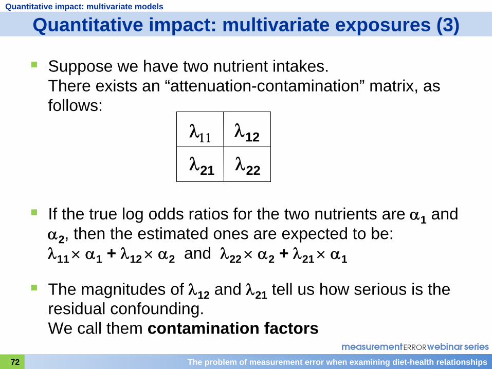
If the true log odds ratios for the two nutrients are 1 and 2 , then the estimated ones are expected to be: 11 1 + 12 2 and 22 2 + 21 1

The magnitudes of 12 and 21 tell us how serious is the residual confounding. We call them contamination factors

Slide 72

Mathematically, the problem is captured by a matrix of four values shown here that we call the attenuation-contamination matrix. If the true log odds ratio for the first dietary intake is alpha-1, then we expect it to be estimated, on average, not as alpha-1 but as lambda-11 times alpha 1 plus lamda-12 times alpha 2. There is a similar expression for the estimate of the log odds ratio for the second dietary variable.

Notice that the first part of the expression lambda-11 times alpha-1 is exactly the same as the attenuation expression that we saw for a single variable. The second part of the expression, lambda-12 times alpha-2, is the new part—the residual confounding introduced by the entry of a second dietary variable into the regression. For this reason, the off-diagonal terms of the matrix lamda-12 and lamda-21 tell us how serious the residual confounding is; we call them contamination factors.




I

f 12 and 21 are small, then the only bias in the estimated log odds ratios comes essentially from attenuation, then:

a) The estimated log odds ratio is attenuated

b) The significance test is valid

So we need to know for dietary data, how large are the contamination factors

We can estimate them from the OPEN study

Slide 73

If these contamination factors are very small, then the only effective bias in the estimated log odds ratios is essentially one of attenuation. The situation reverts to the one we had earlier with a single error-prone variable in the regression model. The log odds ratio is attenuated and the significance test is valid, although less powerful.

So we need to know the values of contamination factors to understand whether we need to be concerned about residual confounding. Fortunately, we can estimate some of them from the OPEN study.




OPEN – Estimated Contamination Factors(Freedman, Schatzkin, Midthune, Kipnis, J Nat Cancer Inst 2011)

Dietary Component Gender Protein Density Potassium

Density Energy

Energy Men -0.01 (0.03) 0.13 (0.05) -

Energy Women 0.03 (0.05) 0.10 (0.06) -

Protein Density Men - -0.01 (0.09) 0.08 (0.05)

Protein Women - 0.00 (0.10) 0.06 (0.05)

Potass. Density Men -0.05 (0.06) - 0.04 (0.04)

Potassium Women 0.00 (0.07) - -0.04 (0.05)

Total Fat Density Men -0.03 (0.07) 0.00 (0.08) 0.05 (0.05)

Total Fat Women -0.02 (0.08) -0.08 (0.10) -0.07 (0.05)

Sat. Fat Density Men -0.03 (0.05) -0.04 (0.07) 0.10 (0.04)

Saturated Fat Women -0.01 (0.06) -0.07 (0.08) -0.02 (0.04)

Slide 74

In this slide we see the estimates for a selected set of nutrients. Because of the restricted set of recovery biomarkers, we can investigate only pairs of nutrients, of which at least one is energy, protein, or potassium, or their densities. You can see from this table that the values for the contamination factors are all small, the largest amongst this set of 24 values being 0.13.




OPEN: Contamination factors

–

–

Contamination factors generally appear small, meaning that residual confounding does not appear to be a serious problem

However, note that OPEN and other recovery biomarker validation studies examine only energy, protein and potassium

Similar findings for other nutrients cannot be guaranteed

Slide 75

The conclusion, therefore, based on current evidence is that residual confounding is not a major source of bias in odds ratio estimates. However, the evidence is restricted by the limited number of recovery biomarkers available, and we cannot be totally sure that it applies to pairs of nutrients outside our restricted sets.


SUMMARY

Slide 76

[No notes.]


Summary

Summary

1. Errors in self-reported dietary intake have a complex structure including systematic biases, person-specific biases and within-person random error

2. The person-specific biases and within-person random error have a profound impact on the estimation of disease risk parameters such as the log odds ratio. Estimates of these are severely attenuated

3. For a FFQ, these effects can be partially mitigated by energy-adjustment

4. The same biases and random errors also cause loss of statistical power for detecting diet-health relationships

Slide 77

[No notes.]


Summary

What’s coming next?

In the next lecture, we will study how we can correct the attenuation in the estimated disease risk parameter

This will require us to learn about calibration studies and also a neat statistical method known as regression calibration

Slide 78

[No notes.]


QUESTIONS & ANSWERSModerator: Sharon Kirkpatrick

Please submit questions using the Chat function

Slide 79

Thank you Dr. Freedman. We’ll now move on to the question and answer period of the webinar.

Measurement Error Webinar 6 Q&A

Question: Could you please comment on whether the concepts that you’ve discussed apply when diet is the outcome rather than the exposure?

The answer is that there are effects and impacts of dietary measurement error when the dietary variable is the outcome and not the exposure variable, but they are different. Essentially what happens is that the regression coefficients are still biased but the bias is only impacted by the multiplicative, systematic bias parameter β1 and the estimated regression coefficient is equal to β1 times the true value. So they are attenuated as much as β1 is, but they’re not impacted by person-specific biases or by within-person random error. The person-specific biases and within-person random error do, however, increase the variance of the residual in the regression model and, therefore, do reduce power to detect the effect. (L. Freedman)

Will the series cover methods related to diet and health relationships using both FFQ data and 24 hour recall data?

The series will indeed look at 24 hour recall data. There is a specific problem with 24 hour recall data in that, often, with nutrients or foods that are not regularly consumed, they lead to data which have large numbers of zeros in them. And I believe that Dr. Kipnis will cover that particular issue and that problem later on in this series. (L. Freedman)

Is there a preferred method of energy adjustment or does it depend on the situation?

It does very much depend on the situation. One particular aspect that comes up in the choice of which method to use is what sort of variable you are using as your dietary variable—whether you are using a continuous variable or whether you’re using a categorized variable. For example, if you are using a continuous variable, it actually doesn’t make any difference at all whether you use the standard method or another method which I haven’t described, which is called the residual method. They lead to exactly the same answers. But if you categorize your variables, it’s been shown that the residual method is better than the standard method and leads to less-biased results. So it does very much depend on exactly which model you’re using to analyze the data in terms of your variables, which type of variable you’re using, and other aspects as well. And there’s also a certain subjective element. Some people really like using nutrient

densities—I’m one of them—and prefer to use the density method because of that. They find it easier to explain the results that way. So there is a certain amount of personal choice involved as well. (L. Freedman)

How do the results of OPEN compare to those of other biomarker studies?

We’re actually conducting, at the moment, a pooling study, which includes OPEN together with three other large validation studies with recovery biomarkers which have been carried out subsequently. Some of them have been already reported; one is the AMPM study of the USDA, and the other one that has been reported is the NBS study of the Women’s Health Initiative. And you can actually go and look up the results in those published studies. You will find that, for the most part, the results are quite comparable with OPEN. There are some small differences here and there but, generally speaking, results are fairly consistent. (L. Freedman)

This question relates to dietary assessments. Usually, an FFQ asks about usual intake while a 24 hour recall covers short-term intake. If biomarkers capture short-term intake, can they still tell us about error in the FFQ?

I believe they can, yes, because even though dietary biomarkers measure short-term intake, if they are recovery biomarkers and they are unbiased, and if we assume there is not very much change over time nor large time trends in intakes, then several biomarkers, repeat biomarkers, should indeed capture usual intake over a longer period. And, therefore, they can still be used through statistical modeling to evaluate the food frequency questionnaire, which is of course aimed at measuring long-term usual intake. So the answer is, yes, I do believe they can be used for that purpose. (L. Freedman)

Could you elaborate on the differences between recovery and concentration biomarkers?

The difference between recovery and concentration biomarkers is a topic that’s been discussed much in the literature and I’m sure you can find papers, especially those of Rudolph Kaaks, which go into this in great detail. In essence, the difference between the two for our purposes are that the recovery biomarkers, as I explained in the lecture, are thought and have been shown to have the properties that are very desirable for evaluating questionnaires in that they are unbiased and they do not have errors that are related to the errors in the questionnaire. Concentration

biomarkers are generally biased measures which do not directly reflect the intake of a particular nutrient, although they may be related, correlated, to that intake. So you can’t use them directly as a measure of the intake, because they are subject to complex metabolic processes, and these processes differ in individuals. Then, they often depend on important personal characteristics. An example is with the carotenoids, which are known to be influenced by smoking. And so there are other extraneous variables which impact on them apart from the dietary intake itself, which makes their use and their analysis more complicated as a result. But as I said in the lecture, they can be used to good effect in dietary work, and I’ll be explaining one use in lecture 11 of the series. (L. Freedman)

This is another question on biomarkers. Can you use FFQ or 24 hour recall data to relate dietary intakes to concentration biomarkers?

Well, if the question is can you use them to validate concentration biomarkers or to discover the relation of concentration biomarkers to true usual intake, I think the answer is no, because as we’ve learned today, the self-report instruments themselves are not unbiased measures of dietary intake. The best way of validating a concentration biomarker, and by that I mean discovering its statistical relationship with true intake, is to conduct feeding studies. Such studies have been done for the carotenoids and there is now a very interesting large feeding study which is going on in Seattle where 150 individuals are being fed what has been established as their usual diet, and a whole series of biomarkers are being measured on them over a period of, I think, three weeks. So that should provide us with some very interesting and useful data for future use of concentration biomarkers. (L. Freedman)

[This page intentionally blank.]

Next Session Tuesday, November 1, 2011 10:00-11:30 EDT

Assessing diet-health relationships: Focus on dietary components consumed daily by nearly all persons

Douglas MidthuneNational Cancer Institute

Slide 80

I’d like to thank Dr. Freedman very much and also extend our appreciation to the audience for joining today’s webinar. Please join us next week for webinar 7, when Doug Midthune will discuss methods of accounting for measurement error when assessing relationships between a dietary component consumed daily by most persons and a health outcome.

Documents

Laurence Freedman, PhD, MA Gertner Institute for … · measurement error on the estimation of usual intake distributions in the population. And the second concerns the impact of