Embed Size (px)
Citation preview

Lattices and Topology
Guram Bezhanishvili and Mamuka Jibladze
Third Vienna Tbilisi Summer School in Logic and Language27-28.IX.2007

Introduction
Lattice is a particular kind of algebraic structure;
Origins —
George Boole (“An Investigation of the Laws of Thought...”,1854)
Richard Dedekind (Series of papers, ∼ 1900)
Importance for logic —
Lattices encode algebraically behavior of the entailmentrelation and basic logical connectives “and” (&, ∧,conjunction), “or” (∨, disjunction) between propositions.
Relationship between logical syntax and semantics islikewise reflected in the relationship between lattices andtheir dual spaces.
Duals are used to provide various useful representationtheorems for lattices, which reflect various completenessresults in logic.

Introduction
Lattice is a particular kind of algebraic structure;Origins —
George Boole (“An Investigation of the Laws of Thought...”,1854)
Richard Dedekind (Series of papers, ∼ 1900)
Importance for logic —
Lattices encode algebraically behavior of the entailmentrelation and basic logical connectives “and” (&, ∧,conjunction), “or” (∨, disjunction) between propositions.
Relationship between logical syntax and semantics islikewise reflected in the relationship between lattices andtheir dual spaces.
Duals are used to provide various useful representationtheorems for lattices, which reflect various completenessresults in logic.

Introduction
Our aim is to give a systematic yet elementary account of theessentials of lattice theory and its connection to topology.
After providing the necessary prerequisites, we will tell aboutthe dual spaces of distributive lattices, and the representationtheorems provided by the duality.
The logical significance of these theorems lies in the fact thatthey are essentially equivalent to results about completeness ofcertain intermediate logics with respect to the topologicalsemantics.

Outline
Lecture 1 Partial orders.Lattices and complete lattices.Lattices as algebras.
Lecture 2 Distributive laws.Birkhoff’s characterization of distributive lattices.Duality between finite distributive lattices and finite posets.
Lecture 3 Topologies.Frames.Sober spaces and spatial frames.
Lecture 4 Coherent frames.Spectral spaces and Stone duality.Priestley duality.

Posets
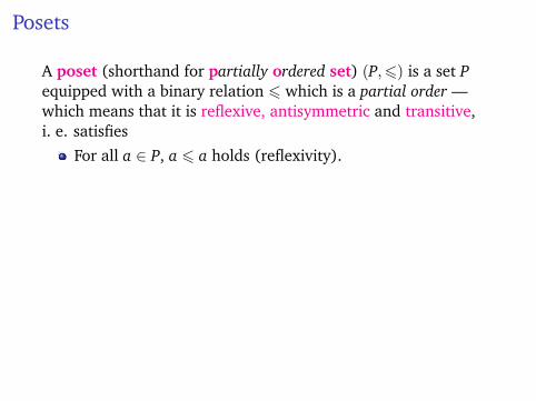
A poset (shorthand for partially ordered set) (P,6) is a set Pequipped with a binary relation 6 which is a partial order —which means that it is reflexive, antisymmetric and transitive
,i. e. satisfies
For all a ∈ P, a 6 a holds (reflexivity).
For all a, b ∈ P, if both a 6 b and b 6 a hold, then a = b(antisymmetry).
For all a, b, c ∈ P, if a 6 b and b 6 c holds, then a 6 c holdstoo (transitivity).
We will write “b > a” to mean the same as “a 6 b”; moreover“a < b” will be shorthand notation for “a 6 b and a 6= b”.
Sometimes we will just refer to a poset as “P” instead of“(P,6)”, when “6” is clear from the context.
Posets
A poset (shorthand for partially ordered set) (P,6) is a set Pequipped with a binary relation 6 which is a partial order —which means that it is reflexive, antisymmetric and transitive,i. e. satisfies
For all a ∈ P, a 6 a holds (reflexivity).
For all a, b ∈ P, if both a 6 b and b 6 a hold, then a = b(antisymmetry).
For all a, b, c ∈ P, if a 6 b and b 6 c holds, then a 6 c holdstoo (transitivity).
We will write “b > a” to mean the same as “a 6 b”; moreover“a < b” will be shorthand notation for “a 6 b and a 6= b”.
Sometimes we will just refer to a poset as “P” instead of“(P,6)”, when “6” is clear from the context.

Hasse diagrams. Examples.
There is a very useful way to depict posets using the so calledHasse diagrams. It is based on the following simple fact.
Let a � b mean that a < b and there is no c with a < c < b. Wewill then say that a covers b.
It is clear that in a finite poset, a 6 b holds if and only ifeither a = b, or
a � c1 � c2 � · · · � cn � b
for some c1, ..., cn ∈ P (n > 0).
Thus we can fully describe a finite poset by specifying thecovering relation only, instead of the whole 6. This can be donegraphically; to indicate a � b, one pictures a somewhere belowb, and joins them with a line.

Hasse diagrams. Examples.
There is a very useful way to depict posets using the so calledHasse diagrams. It is based on the following simple fact.
Let a � b mean that a < b and there is no c with a < c < b. Wewill then say that a covers b.
It is clear that in a finite poset, a 6 b holds if and only if
either a = b, ora � c1 � c2 � · · · � cn � b
for some c1, ..., cn ∈ P (n > 0).
Thus we can fully describe a finite poset by specifying thecovering relation only, instead of the whole 6. This can be donegraphically; to indicate a � b, one pictures a somewhere belowb, and joins them with a line.

Hasse diagrams. Examples.
There is a very useful way to depict posets using the so calledHasse diagrams. It is based on the following simple fact.
Let a � b mean that a < b and there is no c with a < c < b. Wewill then say that a covers b.
It is clear that in a finite poset, a 6 b holds if and only ifeither a = b, or
a � c1 � c2 � · · · � cn � b
for some c1, ..., cn ∈ P (n > 0).
Thus we can fully describe a finite poset by specifying thecovering relation only, instead of the whole 6. This can be donegraphically; to indicate a � b, one pictures a somewhere belowb, and joins them with a line.

Hasse diagrams. Examples.
There is a very useful way to depict posets using the so calledHasse diagrams. It is based on the following simple fact.
Let a � b mean that a < b and there is no c with a < c < b. Wewill then say that a covers b.
It is clear that in a finite poset, a 6 b holds if and only ifeither a = b, or
a � c1 � c2 � · · · � cn � b
for some c1, ..., cn ∈ P (n > 0).
Thus we can fully describe a finite poset by specifying thecovering relation only, instead of the whole 6. This can be donegraphically; to indicate a � b, one pictures a somewhere belowb, and joins them with a line.

Hasse diagrams. Examples.For example, consider P = {a, b, c, d, e} with
a 6 a a 6 b a 6 c a 6 d a 6 eb 6 b b 6 d b 6 e
c 6 c c 6 d c 6 ed 6 d
e 6 e.
Then, this whole relation can be encoded in the correspondingHasse diagram
d e
b
��������������c
??????????????
a
??????������

Hasse diagrams. Examples.For example, consider P = {a, b, c, d, e} with
a 6 a a 6 b a 6 c a 6 d a 6 eb 6 b b 6 d b 6 e
c 6 c c 6 d c 6 ed 6 d
e 6 e.
Then, this whole relation can be encoded in the correspondingHasse diagram
d e
b
��������������c
??????????????
a
??????������

Hasse diagrams. Examples.
Any set P whatsoever can be equipped with a simplest (and leastinteresting) partial order — the discrete one “6”=“=”. That is,in (P,=) one has a 6 b if and only if a = b.
The corresponding Hasse diagram does not thus have any lines,and looks like
• • • • •

Hasse diagrams. Examples.
Any set P whatsoever can be equipped with a simplest (and leastinteresting) partial order — the discrete one “6”=“=”. That is,in (P,=) one has a 6 b if and only if a = b.
The corresponding Hasse diagram does not thus have any lines,and looks like
• • • • •
Hasse diagrams. Examples.
Any set P of real numbers produces a poset by taking the usualorder for “6”. This order will be always total, i. e. will satisfy
for all a, b ∈ P, either a 6 b or b 6 a holds.
Total orders are also called linear. Their Hasse diagrams looklike
•••••

Hasse diagrams. Examples.
Any set P of real numbers produces a poset by taking the usualorder for “6”. This order will be always total, i. e. will satisfy
for all a, b ∈ P, either a 6 b or b 6 a holds.
Total orders are also called linear. Their Hasse diagrams looklike
•••••

Hasse diagrams. Examples.
For a poset (P,6) its opposite is (P,>). Indeed obviously 6 is apartial order iff > is. Dual of P will be denoted by P◦.
The Hasse diagram of P◦ can be obtained from that of P byturning it upside down.
For a poset (P,6), any subset P′ ⊆ P can be equipped with theinduced partial order 6′=6|P′ by declaring a′ 6′ b′ for a′, b′ ∈ P′
if and only if a′ 6 b′ in P. In such circumstances, we will saythat (P′,6′) is a subposet of (P,6).
For posets (P1,61), ..., (Pn,6n), the disjoint union P1 t · · · t Pncan be equipped with a natural partial order 6 by declaring, fora ∈ Pi and b ∈ Pj, “a 6 b” to mean “i = j and a 6i b”. Thecorresponding Hasse diagram will look like disjoint union of theHasse diagrams of the Pi’s.

Hasse diagrams. Examples.
Moreover, for posets (P1,61), ..., (Pn,6n) there is a naturalpartial order 6 on the Cartesian product P1 × · · · × Pn, definedby declaring (a1, ..., an) 6 (b1, ..., bn) to hold if and only ifai 6i bi for all i = 1, ...,n.
For example,
c
a
��������b
=======×
e
d
=
(c, e)
(a, e)
wwwwwwww(c, d) (b, e)
GGGGGGGG
(a, d)
wwwwwwww(b, d)
GGGGGGGG
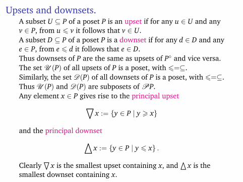
Upsets and downsets.A subset U ⊆ P of a poset P is an upset if for any u ∈ U and anyv ∈ P, from u 6 v it follows that v ∈ U.
A subset D ⊆ P of a poset P is a downset if for any d ∈ D and anye ∈ P, from e 6 d it follows that e ∈ D.Thus downsets of P are the same as upsets of P◦ and vice versa.The set U (P) of all upsets of P is a poset, with 6=⊆.Similarly, the set D(P) of all downsets of P is a poset, with 6=⊆.Thus U (P) and D(P) are subposets of PP.Any element x ∈ P gives rise to the principal upset
hx := {y ∈ P | y > x}
and the principal downseti
x := {y ∈ P | y 6 x} .
Clearly`
x is the smallest upset containing x, anda
x is thesmallest downset containing x.

Upsets and downsets.A subset U ⊆ P of a poset P is an upset if for any u ∈ U and anyv ∈ P, from u 6 v it follows that v ∈ U.A subset D ⊆ P of a poset P is a downset if for any d ∈ D and anye ∈ P, from e 6 d it follows that e ∈ D.
Thus downsets of P are the same as upsets of P◦ and vice versa.The set U (P) of all upsets of P is a poset, with 6=⊆.Similarly, the set D(P) of all downsets of P is a poset, with 6=⊆.Thus U (P) and D(P) are subposets of PP.Any element x ∈ P gives rise to the principal upset
hx := {y ∈ P | y > x}
and the principal downseti
x := {y ∈ P | y 6 x} .
Clearly`
x is the smallest upset containing x, anda
x is thesmallest downset containing x.

Upsets and downsets.A subset U ⊆ P of a poset P is an upset if for any u ∈ U and anyv ∈ P, from u 6 v it follows that v ∈ U.A subset D ⊆ P of a poset P is a downset if for any d ∈ D and anye ∈ P, from e 6 d it follows that e ∈ D.Thus downsets of P are the same as upsets of P◦ and vice versa.
The set U (P) of all upsets of P is a poset, with 6=⊆.Similarly, the set D(P) of all downsets of P is a poset, with 6=⊆.Thus U (P) and D(P) are subposets of PP.Any element x ∈ P gives rise to the principal upset
hx := {y ∈ P | y > x}
and the principal downseti
x := {y ∈ P | y 6 x} .
Clearly`
x is the smallest upset containing x, anda
x is thesmallest downset containing x.

Upsets and downsets.A subset U ⊆ P of a poset P is an upset if for any u ∈ U and anyv ∈ P, from u 6 v it follows that v ∈ U.A subset D ⊆ P of a poset P is a downset if for any d ∈ D and anye ∈ P, from e 6 d it follows that e ∈ D.Thus downsets of P are the same as upsets of P◦ and vice versa.The set U (P) of all upsets of P is a poset, with 6=⊆.
Similarly, the set D(P) of all downsets of P is a poset, with 6=⊆.Thus U (P) and D(P) are subposets of PP.Any element x ∈ P gives rise to the principal upset
hx := {y ∈ P | y > x}
and the principal downseti
x := {y ∈ P | y 6 x} .
Clearly`
x is the smallest upset containing x, anda
x is thesmallest downset containing x.

Upsets and downsets.A subset U ⊆ P of a poset P is an upset if for any u ∈ U and anyv ∈ P, from u 6 v it follows that v ∈ U.A subset D ⊆ P of a poset P is a downset if for any d ∈ D and anye ∈ P, from e 6 d it follows that e ∈ D.Thus downsets of P are the same as upsets of P◦ and vice versa.The set U (P) of all upsets of P is a poset, with 6=⊆.Similarly, the set D(P) of all downsets of P is a poset, with 6=⊆.
Thus U (P) and D(P) are subposets of PP.Any element x ∈ P gives rise to the principal upset
hx := {y ∈ P | y > x}
and the principal downseti
x := {y ∈ P | y 6 x} .
Clearly`
x is the smallest upset containing x, anda
x is thesmallest downset containing x.

Upsets and downsets.A subset U ⊆ P of a poset P is an upset if for any u ∈ U and anyv ∈ P, from u 6 v it follows that v ∈ U.A subset D ⊆ P of a poset P is a downset if for any d ∈ D and anye ∈ P, from e 6 d it follows that e ∈ D.Thus downsets of P are the same as upsets of P◦ and vice versa.The set U (P) of all upsets of P is a poset, with 6=⊆.Similarly, the set D(P) of all downsets of P is a poset, with 6=⊆.Thus U (P) and D(P) are subposets of PP.
Any element x ∈ P gives rise to the principal upseth
x := {y ∈ P | y > x}
and the principal downseti
x := {y ∈ P | y 6 x} .
Clearly`
x is the smallest upset containing x, anda
x is thesmallest downset containing x.
Upsets and downsets.A subset U ⊆ P of a poset P is an upset if for any u ∈ U and anyv ∈ P, from u 6 v it follows that v ∈ U.A subset D ⊆ P of a poset P is a downset if for any d ∈ D and anye ∈ P, from e 6 d it follows that e ∈ D.Thus downsets of P are the same as upsets of P◦ and vice versa.The set U (P) of all upsets of P is a poset, with 6=⊆.Similarly, the set D(P) of all downsets of P is a poset, with 6=⊆.Thus U (P) and D(P) are subposets of PP.Any element x ∈ P gives rise to the principal upset
hx := {y ∈ P | y > x}
and the principal downseti
x := {y ∈ P | y 6 x} .
Clearly`
x is the smallest upset containing x, anda
x is thesmallest downset containing x.

Suprema and infima.
An element x ∈ P is maximal if`
x = {x} and minimal ifax = {x}.
A largest or top element in a poset (P,6) is an element > ∈ Pwhich is a unique maximal element.
A least or bottom element is a ⊥ ∈ P which is a unique minimalelement.
An upper bound for a subset S ⊆ P in a poset (P,6) is anelement u ∈ P with s 6 u for all s ∈ S.
A lower bound for S is an element l ∈ P with l 6 s for all s ∈ S.

Suprema and infima.
For any set S,
S↑ := {u ∈ P | u is an upper bound for S}
is an upset, and
S↓ := {d ∈ P | d is a lower bound for S}
is a downset.
We say that S ⊆ P possesses the least upper bound (shortly lub),or supremum, or join, if S↑ has a bottom
∨S.
We say that S ⊆ P possesses the greatest lower bound (shortlyglb), or infimum, or meet, if S↓ has a top
∧S.
Note that it follows from this definition that∨
∅ is a bottomelement, and
∧∅ is a top element (if they exist).

Suprema and infima.
In particular, we denote by a ∨ b, for elements a, b ∈ P the join∨{a, b} of the two element set {a, b}. It is thus an element (if it
exists) such that a 6 a ∨ b, b 6 a ∨ b, and for any other u ∈ Pwith a 6 u and b 6 u, one has a ∨ b 6 u.
Dually, we denote by a ∧ b the meet∧{a, b} of {a, b}. It is thus
an element (if it exists) such that a ∧ b 6 a, a ∧ b 6 b, and forany other l ∈ P with l 6 a and l 6 b, one must have l 6 a ∧ b.

Lattices.
A lattice L is a poset in which any two elements a, b ∈ L possessboth join a ∨ b and meet a ∧ b.
Here are Hasse diagrams of some finite lattices:
•
•
~~~~~~~• •
@@@@@@@
•
~~~~~~~
@@@@@@@
,
•
•
•
~~~~~~~•
@@@@@@@
•
~~~~~~~
@@@@@@@

Lattices.
A lattice L is a poset in which any two elements a, b ∈ L possessboth join a ∨ b and meet a ∧ b.
Here are Hasse diagrams of some finite lattices:
•
•
~~~~~~~• •
@@@@@@@
•
~~~~~~~
@@@@@@@
,
•
•
•
~~~~~~~•
@@@@@@@
•
~~~~~~~
@@@@@@@
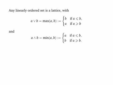
Any linearly ordered set is a lattice, with
a ∨ b = max(a, b) :=
{b if a 6 b,a if a > b
and
a ∧ b = min(a, b) :=
{a if a 6 b,b if a > b.
The following posets, however, are not lattices:
•
•
~~~~~~~•
@@@@@@@,
• •
•
~~~~~~~
@@@@@@@,
• •
•
~~~~~~~•
@@@@@@@

Any linearly ordered set is a lattice, with
a ∨ b = max(a, b) :=
{b if a 6 b,a if a > b
and
a ∧ b = min(a, b) :=
{a if a 6 b,b if a > b.
The following posets, however, are not lattices:
•
•
~~~~~~~•
@@@@@@@,
• •
•
~~~~~~~
@@@@@@@,
• •
•
~~~~~~~•
@@@@@@@

Lattices.
In a lattice L, all nonempty finite subsets possess suprema andinfima.
Indeed, it is easy to see that one has∨{a1, a2, ..., an} = (...(a1 ∨ a2) ∨ ...) ∨ an
and ∧{a1, a2, ..., an} = (...(a1 ∧ a2) ∧ ...) ∧ an.

Lattices.
In a lattice L, all nonempty finite subsets possess suprema andinfima.
Indeed, it is easy to see that one has∨{a1, a2, ..., an} = (...(a1 ∨ a2) ∨ ...) ∨ an
and ∧{a1, a2, ..., an} = (...(a1 ∧ a2) ∧ ...) ∧ an.

Complete lattices.
A complete lattice L is one possessing suprema and infima for allsubsets.
For example, the interval [0,1] with the usual (linear) orderingforms a complete lattice.
The powerset PX of any set X is a complete lattice with respectto the order 6=⊆. Indeed for any S ⊆PX one then has∨
S =⋃
S and∧
S =⋂
S.
Note however that the set PfinX of finite subsets of X equippedwith the same order is a complete lattice if and only if X is finite.
Lattices as algebraic structures.
It turns out that one can equivalently define the structure oflattice on a set purely in terms of the binary operations ∧ and ∨.
Note that in a lattice ∨ and ∧ satisfy the following identities:1 a ∨ a = a = a ∧ a (idempotency);2 a ∧ (a ∨ b) = a = a ∨ (a ∧ b) (absorption);3 a ∨ b = b ∨ a and a ∧ b = b ∧ a (commutativity);4 (a ∨ b) ∨ c = a ∨ (b ∨ c) and (a ∧ b) ∧ c = a ∧ (b ∧ c)
(associativity).

Lattices as algebraic structures.
It turns out that one can equivalently define the structure oflattice on a set purely in terms of the binary operations ∧ and ∨.
Note that in a lattice ∨ and ∧ satisfy the following identities:1 a ∨ a = a = a ∧ a (idempotency);
2 a ∧ (a ∨ b) = a = a ∨ (a ∧ b) (absorption);3 a ∨ b = b ∨ a and a ∧ b = b ∧ a (commutativity);4 (a ∨ b) ∨ c = a ∨ (b ∨ c) and (a ∧ b) ∧ c = a ∧ (b ∧ c)
(associativity).

Lattices as algebraic structures.
It turns out that one can equivalently define the structure oflattice on a set purely in terms of the binary operations ∧ and ∨.
Note that in a lattice ∨ and ∧ satisfy the following identities:1 a ∨ a = a = a ∧ a (idempotency);2 a ∧ (a ∨ b) = a = a ∨ (a ∧ b) (absorption);
3 a ∨ b = b ∨ a and a ∧ b = b ∧ a (commutativity);4 (a ∨ b) ∨ c = a ∨ (b ∨ c) and (a ∧ b) ∧ c = a ∧ (b ∧ c)
(associativity).

Lattices as algebraic structures.
It turns out that one can equivalently define the structure oflattice on a set purely in terms of the binary operations ∧ and ∨.
Note that in a lattice ∨ and ∧ satisfy the following identities:1 a ∨ a = a = a ∧ a (idempotency);2 a ∧ (a ∨ b) = a = a ∨ (a ∧ b) (absorption);3 a ∨ b = b ∨ a and a ∧ b = b ∧ a (commutativity);
4 (a ∨ b) ∨ c = a ∨ (b ∨ c) and (a ∧ b) ∧ c = a ∧ (b ∧ c)(associativity).

Lattices as algebraic structures.
It turns out that one can equivalently define the structure oflattice on a set purely in terms of the binary operations ∧ and ∨.
Note that in a lattice ∨ and ∧ satisfy the following identities:1 a ∨ a = a = a ∧ a (idempotency);2 a ∧ (a ∨ b) = a = a ∨ (a ∧ b) (absorption);3 a ∨ b = b ∨ a and a ∧ b = b ∧ a (commutativity);4 (a ∨ b) ∨ c = a ∨ (b ∨ c) and (a ∧ b) ∧ c = a ∧ (b ∧ c)
(associativity).
Lattices as algebraic structures.
Conversely, suppose given a set L equipped with two binaryoperations ∧,∨ : L× L→ L satisfying the above identities.
Then we can define
a 6∧,∨ b if and only if a ∧ b = a if and only if a ∨ b = b.
It is easy to show that this is a partial order.

Lattices as algebraic structures.
Conversely, suppose given a set L equipped with two binaryoperations ∧,∨ : L× L→ L satisfying the above identities.
Then we can define
a 6∧,∨ b if and only if a ∧ b = a if and only if a ∨ b = b.
It is easy to show that this is a partial order.

Lattices as algebraic structures.
We can now go in two different rounds.First, let us start with a lattice (L,6).
It gives rise to the algebraic structure (L,∧,∨) defined as above.
From this, we have just constructed another partial order, so weget another lattice (L,6∧,∨).
Fact. This is the same lattice that we started with. That is,6∧,∨=6.

Lattices as algebraic structures.
For the second round, let us start with an algebraic structure(L,∨,∧) satisfying 1.-4. above.
It gives rise to a lattice (L,6∧,∨) defined as above.
Fact. This is a lattice, with ∨ and ∧ serving as binary suprema,resp. infima.

Lattices as algebraic structures.
For the second round, let us start with an algebraic structure(L,∨,∧) satisfying 1.-4. above.
It gives rise to a lattice (L,6∧,∨) defined as above.
Fact. This is a lattice, with ∨ and ∧ serving as binary suprema,resp. infima.

Lattices as algebraic structures.
For the second round, let us start with an algebraic structure(L,∨,∧) satisfying 1.-4. above.
It gives rise to a lattice (L,6∧,∨) defined as above.
Fact. This is a lattice, with ∨ and ∧ serving as binary suprema,resp. infima.

Producing new lattices.
Disjoint union of lattices is almost never a lattice.
In fact, assoon as P1, P2 6= ∅, the poset P1 t P2 cannot be a lattice: noelements a1 ∈ P1, a2 ∈ P2 have any common upper or lowerbounds.
On the other hand, any product L1 × ...× Ln of lattices is again alattice. In fact, it is easy to check that one has
(a1 ∨ b1, ..., an ∨ bn) = (a1, ..., an) ∨ (b1, ..., bn),
and similarly for ∧.

Producing new lattices.
Disjoint union of lattices is almost never a lattice. In fact, assoon as P1, P2 6= ∅, the poset P1 t P2 cannot be a lattice: noelements a1 ∈ P1, a2 ∈ P2 have any common upper or lowerbounds.
On the other hand, any product L1 × ...× Ln of lattices is again alattice.
In fact, it is easy to check that one has
(a1 ∨ b1, ..., an ∨ bn) = (a1, ..., an) ∨ (b1, ..., bn),
and similarly for ∧.

Producing new lattices.
Disjoint union of lattices is almost never a lattice. In fact, assoon as P1, P2 6= ∅, the poset P1 t P2 cannot be a lattice: noelements a1 ∈ P1, a2 ∈ P2 have any common upper or lowerbounds.
On the other hand, any product L1 × ...× Ln of lattices is again alattice. In fact, it is easy to check that one has
(a1 ∨ b1, ..., an ∨ bn) = (a1, ..., an) ∨ (b1, ..., bn),
and similarly for ∧.

Sublattices, filters, ideals.
A subposet L′ ⊆ L of a lattice L is called a sublattice if it is closedunder the operations ∨, ∧.
In other words, L′ is a sublattice if for any a, b ∈ L, from a, b ∈ L′
follows a ∨ b, a ∧ b ∈ L′.
A sublattice F ⊆ L is a filter if a stronger condition is satisfied:for any a, b ∈ L, just from a ∈ F only it follows a ∨ b ∈ F.
The dual notion to that of filter is the notion of ideal. Asublattice I ⊆ L is an ideal if for any a, b ∈ L, from a ∈ I only itfollows a ∧ b ∈ I.

Sublattices, filters, ideals.
A subposet L′ ⊆ L of a lattice L is called a sublattice if it is closedunder the operations ∨, ∧.In other words, L′ is a sublattice if for any a, b ∈ L, from a, b ∈ L′
follows a ∨ b, a ∧ b ∈ L′.
A sublattice F ⊆ L is a filter if a stronger condition is satisfied:
for any a, b ∈ L, just from a ∈ F only it follows a ∨ b ∈ F.
The dual notion to that of filter is the notion of ideal. Asublattice I ⊆ L is an ideal if for any a, b ∈ L, from a ∈ I only itfollows a ∧ b ∈ I.

Sublattices, filters, ideals.
A subposet L′ ⊆ L of a lattice L is called a sublattice if it is closedunder the operations ∨, ∧.In other words, L′ is a sublattice if for any a, b ∈ L, from a, b ∈ L′
follows a ∨ b, a ∧ b ∈ L′.
A sublattice F ⊆ L is a filter if a stronger condition is satisfied:for any a, b ∈ L, just from a ∈ F only it follows a ∨ b ∈ F.
The dual notion to that of filter is the notion of ideal. Asublattice I ⊆ L is an ideal if for any a, b ∈ L, from a ∈ I only itfollows a ∧ b ∈ I.

Sublattices, filters, ideals.
A subposet L′ ⊆ L of a lattice L is called a sublattice if it is closedunder the operations ∨, ∧.In other words, L′ is a sublattice if for any a, b ∈ L, from a, b ∈ L′
follows a ∨ b, a ∧ b ∈ L′.
A sublattice F ⊆ L is a filter if a stronger condition is satisfied:for any a, b ∈ L, just from a ∈ F only it follows a ∨ b ∈ F.
The dual notion to that of filter is the notion of ideal.
Asublattice I ⊆ L is an ideal if for any a, b ∈ L, from a ∈ I only itfollows a ∧ b ∈ I.

Sublattices, filters, ideals.
A subposet L′ ⊆ L of a lattice L is called a sublattice if it is closedunder the operations ∨, ∧.In other words, L′ is a sublattice if for any a, b ∈ L, from a, b ∈ L′
follows a ∨ b, a ∧ b ∈ L′.
A sublattice F ⊆ L is a filter if a stronger condition is satisfied:for any a, b ∈ L, just from a ∈ F only it follows a ∨ b ∈ F.
The dual notion to that of filter is the notion of ideal. Asublattice I ⊆ L is an ideal if for any a, b ∈ L, from a ∈ I only itfollows a ∧ b ∈ I.

Sublattices, filters, ideals.
Equivalent definitions:
A subset F ⊆ L is a filter if and only if it is a sublattice and anupset.
A subset I ⊆ L is an ideal if and only if it is a sublattice and adownset.
Equivalently, a subset F ⊆ L is a filter if and only if one has
a ∧ b ∈ F ⇐⇒ a ∈ F and b ∈ F
for any a, b ∈ L.
And, a subset I ⊆ L is an ideal if and only if one has
a ∨ b ∈ I ⇐⇒ a ∈ I and b ∈ I.

Sublattices, filters, ideals.
Any subposet of a linearly ordered set is a sublattice.
For any poset P, the subsets U (P),D(P) ⊆PP are sublattices.Neither of them is a filter or an ideal in general.
For any set X, PfinX ⊆PX is an ideal.
Any principal upset is a filter, and any principal downset is anideal.
In a finite lattice, converse is also true. However, PfinX isprincipal if and only if X is finite.
A subposet of a linearly ordered set is a filter if and only if it isan upset, and an ideal if and only if it is a downset.

Prime filters, prime ideals.A filter F ⊆ L is prime if
a ∨ b ∈ F ⇐⇒ a ∈ F or b ∈ F
for any a, b ∈ L.
An ideal I ⊆ L is prime if
a ∧ b ∈ I ⇐⇒ a ∈ I or b ∈ I.
Thus a filter is prime if and only if its complement is an ideal,which is then a prime ideal.Similarly, an ideal is prime if and only if its complement is afilter, which is then a prime filter.Still in other words, for a complemented pair of subsetsU,D ⊆ L, U ∩ D = ∅, U ∪ D = L, the following statements areequivalent:
U is a filter and D is an ideal;U is a prime filter;D is a prime ideal.

Prime filters, prime ideals.A filter F ⊆ L is prime if
a ∨ b ∈ F ⇐⇒ a ∈ F or b ∈ F
for any a, b ∈ L.An ideal I ⊆ L is prime if
a ∧ b ∈ I ⇐⇒ a ∈ I or b ∈ I.
Thus a filter is prime if and only if its complement is an ideal,which is then a prime ideal.
Similarly, an ideal is prime if and only if its complement is afilter, which is then a prime filter.Still in other words, for a complemented pair of subsetsU,D ⊆ L, U ∩ D = ∅, U ∪ D = L, the following statements areequivalent:
U is a filter and D is an ideal;U is a prime filter;D is a prime ideal.

Prime filters, prime ideals.A filter F ⊆ L is prime if
a ∨ b ∈ F ⇐⇒ a ∈ F or b ∈ F
for any a, b ∈ L.An ideal I ⊆ L is prime if
a ∧ b ∈ I ⇐⇒ a ∈ I or b ∈ I.
Thus a filter is prime if and only if its complement is an ideal,which is then a prime ideal.Similarly, an ideal is prime if and only if its complement is afilter, which is then a prime filter.
Still in other words, for a complemented pair of subsetsU,D ⊆ L, U ∩ D = ∅, U ∪ D = L, the following statements areequivalent:
U is a filter and D is an ideal;U is a prime filter;D is a prime ideal.

Prime filters, prime ideals.A filter F ⊆ L is prime if
a ∨ b ∈ F ⇐⇒ a ∈ F or b ∈ F
for any a, b ∈ L.An ideal I ⊆ L is prime if
a ∧ b ∈ I ⇐⇒ a ∈ I or b ∈ I.
Thus a filter is prime if and only if its complement is an ideal,which is then a prime ideal.Similarly, an ideal is prime if and only if its complement is afilter, which is then a prime filter.Still in other words, for a complemented pair of subsetsU,D ⊆ L, U ∩ D = ∅, U ∪ D = L, the following statements areequivalent:
U is a filter and D is an ideal;
U is a prime filter;D is a prime ideal.

Prime filters, prime ideals.A filter F ⊆ L is prime if
a ∨ b ∈ F ⇐⇒ a ∈ F or b ∈ F
for any a, b ∈ L.An ideal I ⊆ L is prime if
a ∧ b ∈ I ⇐⇒ a ∈ I or b ∈ I.
Thus a filter is prime if and only if its complement is an ideal,which is then a prime ideal.Similarly, an ideal is prime if and only if its complement is afilter, which is then a prime filter.Still in other words, for a complemented pair of subsetsU,D ⊆ L, U ∩ D = ∅, U ∪ D = L, the following statements areequivalent:
U is a filter and D is an ideal;U is a prime filter;
D is a prime ideal.

Prime filters, prime ideals.A filter F ⊆ L is prime if
a ∨ b ∈ F ⇐⇒ a ∈ F or b ∈ F
for any a, b ∈ L.An ideal I ⊆ L is prime if
a ∧ b ∈ I ⇐⇒ a ∈ I or b ∈ I.
Thus a filter is prime if and only if its complement is an ideal,which is then a prime ideal.Similarly, an ideal is prime if and only if its complement is afilter, which is then a prime filter.Still in other words, for a complemented pair of subsetsU,D ⊆ L, U ∩ D = ∅, U ∪ D = L, the following statements areequivalent:
U is a filter and D is an ideal;U is a prime filter;D is a prime ideal.

Prime filters, prime ideals.
In a linear order, any upset is not only a filter but even a primefilter, and any downset is a prime ideal.
The above example PfinX ⊆PX is an ideal which is not primeunless X is finite.

Prime filters, prime ideals.
In a linear order, any upset is not only a filter but even a primefilter, and any downset is a prime ideal.
The above example PfinX ⊆PX is an ideal which is not primeunless X is finite.

Distributive laws.
It is easy to see that for any a, b, b′ ∈ L in any lattice L one has
(a ∧ b) ∨ (a ∧ b′) 6 a ∧ (b ∨ b′)
anda ∨ (b ∧ b′) 6 (a ∨ b) ∧ (a ∨ b′).
We will say that in a lattice L, meet distributes over joins, if forany a, b, b′ ∈ L one in fact has
a ∧ (b ∨ b′) = (a ∧ b) ∨ (a ∧ b′).
Dually, join distributes over meets if
a ∨ (b ∧ b′) = (a ∨ b) ∧ (a ∨ b′)
holds.
Distributive laws.These are called the distributive laws. In fact, in any lattice theyare equivalent to each other.
Indeed, suppose
Dxyy′ x ∧ (y ∨ y′) 6 (x ∧ y) ∨ (x ∧ y′)
holds for all x, y, y′ ∈ L.Then for any a, b, b′ ∈ L we have — first using D(a∨b)ab′ —
(a ∨ b) ∧ (a ∨ b′) 6 ((a ∨ b) ∧ a) ∨ ((a ∨ b) ∧ b′)︸ ︷︷ ︸absorption
= a ∨ ((a ∨ b) ∧ b′)︸ ︷︷ ︸Db′ab
6 a ∨ (a ∧ b′) ∨ (b ∧ b′)︸ ︷︷ ︸absorption
= a ∨ (b ∧ b′).

Distributive laws.These are called the distributive laws. In fact, in any lattice theyare equivalent to each other.Indeed, suppose
Dxyy′ x ∧ (y ∨ y′) 6 (x ∧ y) ∨ (x ∧ y′)
holds for all x, y, y′ ∈ L.
Then for any a, b, b′ ∈ L we have — first using D(a∨b)ab′ —
(a ∨ b) ∧ (a ∨ b′) 6 ((a ∨ b) ∧ a) ∨ ((a ∨ b) ∧ b′)︸ ︷︷ ︸absorption
= a ∨ ((a ∨ b) ∧ b′)︸ ︷︷ ︸Db′ab
6 a ∨ (a ∧ b′) ∨ (b ∧ b′)︸ ︷︷ ︸absorption
= a ∨ (b ∧ b′).

Distributive laws.These are called the distributive laws. In fact, in any lattice theyare equivalent to each other.Indeed, suppose
Dxyy′ x ∧ (y ∨ y′) 6 (x ∧ y) ∨ (x ∧ y′)
holds for all x, y, y′ ∈ L.Then for any a, b, b′ ∈ L we have — first using D(a∨b)ab′ —
(a ∨ b) ∧ (a ∨ b′) 6 ((a ∨ b) ∧ a) ∨ ((a ∨ b) ∧ b′)
︸ ︷︷ ︸absorption
= a ∨ ((a ∨ b) ∧ b′)︸ ︷︷ ︸Db′ab
6 a ∨ (a ∧ b′) ∨ (b ∧ b′)︸ ︷︷ ︸absorption
= a ∨ (b ∧ b′).

Distributive laws.These are called the distributive laws. In fact, in any lattice theyare equivalent to each other.Indeed, suppose
Dxyy′ x ∧ (y ∨ y′) 6 (x ∧ y) ∨ (x ∧ y′)
holds for all x, y, y′ ∈ L.Then for any a, b, b′ ∈ L we have — first using D(a∨b)ab′ —
(a ∨ b) ∧ (a ∨ b′) 6 ((a ∨ b) ∧ a) ∨ ((a ∨ b) ∧ b′)︸ ︷︷ ︸absorption
= a ∨ ((a ∨ b) ∧ b′)︸ ︷︷ ︸Db′ab
6 a ∨ (a ∧ b′) ∨ (b ∧ b′)︸ ︷︷ ︸absorption
= a ∨ (b ∧ b′).

Distributive laws.These are called the distributive laws. In fact, in any lattice theyare equivalent to each other.Indeed, suppose
Dxyy′ x ∧ (y ∨ y′) 6 (x ∧ y) ∨ (x ∧ y′)
holds for all x, y, y′ ∈ L.Then for any a, b, b′ ∈ L we have — first using D(a∨b)ab′ —
(a ∨ b) ∧ (a ∨ b′) 6 ((a ∨ b) ∧ a) ∨ ((a ∨ b) ∧ b′)︸ ︷︷ ︸absorption
= a ∨ ((a ∨ b) ∧ b′)
︸ ︷︷ ︸Db′ab
6 a ∨ (a ∧ b′) ∨ (b ∧ b′)︸ ︷︷ ︸absorption
= a ∨ (b ∧ b′).

Distributive laws.These are called the distributive laws. In fact, in any lattice theyare equivalent to each other.Indeed, suppose
Dxyy′ x ∧ (y ∨ y′) 6 (x ∧ y) ∨ (x ∧ y′)
holds for all x, y, y′ ∈ L.Then for any a, b, b′ ∈ L we have — first using D(a∨b)ab′ —
(a ∨ b) ∧ (a ∨ b′) 6 ((a ∨ b) ∧ a) ∨ ((a ∨ b) ∧ b′)︸ ︷︷ ︸absorption
= a ∨ ((a ∨ b) ∧ b′)︸ ︷︷ ︸Db′ab
6 a ∨ (a ∧ b′) ∨ (b ∧ b′)︸ ︷︷ ︸absorption
= a ∨ (b ∧ b′).

Distributive laws.These are called the distributive laws. In fact, in any lattice theyare equivalent to each other.Indeed, suppose
Dxyy′ x ∧ (y ∨ y′) 6 (x ∧ y) ∨ (x ∧ y′)
holds for all x, y, y′ ∈ L.Then for any a, b, b′ ∈ L we have — first using D(a∨b)ab′ —
(a ∨ b) ∧ (a ∨ b′) 6 ((a ∨ b) ∧ a) ∨ ((a ∨ b) ∧ b′)︸ ︷︷ ︸absorption
= a ∨ ((a ∨ b) ∧ b′)︸ ︷︷ ︸Db′ab
6 a ∨ (a ∧ b′) ∨ (b ∧ b′)
︸ ︷︷ ︸absorption
= a ∨ (b ∧ b′).

Distributive laws.These are called the distributive laws. In fact, in any lattice theyare equivalent to each other.Indeed, suppose
Dxyy′ x ∧ (y ∨ y′) 6 (x ∧ y) ∨ (x ∧ y′)
holds for all x, y, y′ ∈ L.Then for any a, b, b′ ∈ L we have — first using D(a∨b)ab′ —
(a ∨ b) ∧ (a ∨ b′) 6 ((a ∨ b) ∧ a) ∨ ((a ∨ b) ∧ b′)︸ ︷︷ ︸absorption
= a ∨ ((a ∨ b) ∧ b′)︸ ︷︷ ︸Db′ab
6 a ∨ (a ∧ b′) ∨ (b ∧ b′)︸ ︷︷ ︸absorption
= a ∨ (b ∧ b′).

Distributive laws.These are called the distributive laws. In fact, in any lattice theyare equivalent to each other.Indeed, suppose
Dxyy′ x ∧ (y ∨ y′) 6 (x ∧ y) ∨ (x ∧ y′)
holds for all x, y, y′ ∈ L.Then for any a, b, b′ ∈ L we have — first using D(a∨b)ab′ —
(a ∨ b) ∧ (a ∨ b′) 6 ((a ∨ b) ∧ a) ∨ ((a ∨ b) ∧ b′)︸ ︷︷ ︸absorption
= a ∨ ((a ∨ b) ∧ b′)︸ ︷︷ ︸Db′ab
6 a ∨ (a ∧ b′) ∨ (b ∧ b′)︸ ︷︷ ︸absorption
= a ∨ (b ∧ b′).

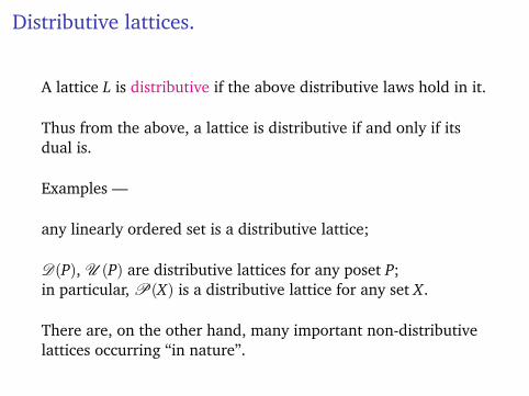
Distributive lattices.
A lattice L is distributive if the above distributive laws hold in it.
Thus from the above, a lattice is distributive if and only if itsdual is.
Examples —
any linearly ordered set is a distributive lattice;
D(P), U (P) are distributive lattices for any poset P;in particular, P(X) is a distributive lattice for any set X.
There are, on the other hand, many important non-distributivelattices occurring “in nature”.

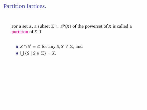
Partition lattices.
For a set X, a subset Σ ⊆P(X) of the powerset of X is called apartition of X if
S ∩ S′ = ∅ for any S, S′ ∈ Σ, and⋃{S | S ∈ Σ} = X.
Let π(X) denote the set of all partitions of X. This set has anatural partial order: for Σ,Σ′ ∈ π(X) we say Σ 6 Σ′ if eachelement of Σ is a union of elements of Σ′.
In fact, π(X) is a complete lattice. However, it is not distributiveas soon as X has more than two elements.

Partition lattices.
For a set X, a subset Σ ⊆P(X) of the powerset of X is called apartition of X if
S ∩ S′ = ∅ for any S, S′ ∈ Σ, and
⋃{S | S ∈ Σ} = X.
Let π(X) denote the set of all partitions of X. This set has anatural partial order: for Σ,Σ′ ∈ π(X) we say Σ 6 Σ′ if eachelement of Σ is a union of elements of Σ′.
In fact, π(X) is a complete lattice. However, it is not distributiveas soon as X has more than two elements.
Partition lattices.
For a set X, a subset Σ ⊆P(X) of the powerset of X is called apartition of X if
S ∩ S′ = ∅ for any S, S′ ∈ Σ, and⋃{S | S ∈ Σ} = X.
Let π(X) denote the set of all partitions of X. This set has anatural partial order: for Σ,Σ′ ∈ π(X) we say Σ 6 Σ′ if eachelement of Σ is a union of elements of Σ′.
In fact, π(X) is a complete lattice. However, it is not distributiveas soon as X has more than two elements.

Partition lattices.
For a set X, a subset Σ ⊆P(X) of the powerset of X is called apartition of X if
S ∩ S′ = ∅ for any S, S′ ∈ Σ, and⋃{S | S ∈ Σ} = X.
Let π(X) denote the set of all partitions of X. This set has anatural partial order: for Σ,Σ′ ∈ π(X) we say Σ 6 Σ′ if eachelement of Σ is a union of elements of Σ′.
In fact, π(X) is a complete lattice. However, it is not distributiveas soon as X has more than two elements.

Partition lattices.
For example, π({1,2,3}) looks like this:
{{1} , {2} , {3}}
{{1} , {2,3}}eeeeeee{{2} , {1,3}} {{3} , {1,2}}
YYYYYYY
{{1,2,3}}YYYYYYYYYY
eeeeeeeeee
Here one has
{{1} {23}} ∧ ({{2} {13}} ∨ {{3} {12}})= {{1} {23}} ∧ {{1} {2} {3}} = {{1} {23}} ,
but
({{1} {23}} ∧ {{2} {13}}) ∨ ({{1} {23}} ∧ {{3} {12}})= {{123}} ∨ {{123}} = {{123}} ,
so distributivity indeed fails.

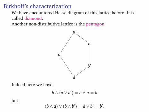
Birkhoff’s characterizationWe have encountered Hasse diagram of this lattice before. It iscalled diamond.
Another non-distributive lattice is the pentagon
u
b
HHHHHHH
a
b′
d
44444444444vvvvvv
Indeed here we have
b ∧ (a ∨ b′) = b ∧ u = b
but(b ∧ a) ∨ (b ∧ b′) = d ∨ b′ = b′.

Birkhoff’s characterizationWe have encountered Hasse diagram of this lattice before. It iscalled diamond.Another non-distributive lattice is the pentagon
u
b
HHHHHHH
a
b′
d
44444444444vvvvvv
Indeed here we have
b ∧ (a ∨ b′) = b ∧ u = b
but(b ∧ a) ∨ (b ∧ b′) = d ∨ b′ = b′.

Birkhoff’s characterizationWe have encountered Hasse diagram of this lattice before. It iscalled diamond.Another non-distributive lattice is the pentagon
u
b
HHHHHHH
a
b′
d
44444444444vvvvvv
Indeed here we have
b ∧ (a ∨ b′) = b ∧ u = b
but(b ∧ a) ∨ (b ∧ b′) = d ∨ b′ = b′.
Birkhoff’s characterizationWe have encountered Hasse diagram of this lattice before. It iscalled diamond.Another non-distributive lattice is the pentagon
u
b
HHHHHHH
a
b′
d
44444444444vvvvvv
Indeed here we have
b ∧ (a ∨ b′) = b ∧ u = b
but(b ∧ a) ∨ (b ∧ b′) = d ∨ b′ = b′.
Birkhoff’s characterization
Theorem (Birkhoff). A lattice is distributive if and only if thereare no diamonds or pentagons among its sublattices.

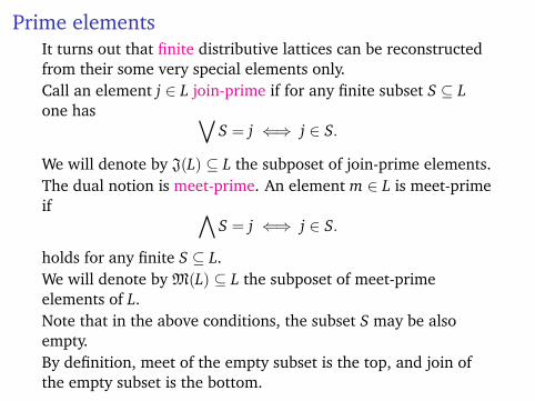
Prime elementsIt turns out that finite distributive lattices can be reconstructedfrom their some very special elements only.
Call an element j ∈ L join-prime if for any finite subset S ⊆ Lone has ∨
S = j ⇐⇒ j ∈ S.
We will denote by J(L) ⊆ L the subposet of join-prime elements.The dual notion is meet-prime. An element m ∈ L is meet-primeif ∧
S = j ⇐⇒ j ∈ S.
holds for any finite S ⊆ L.We will denote by M(L) ⊆ L the subposet of meet-primeelements of L.Note that in the above conditions, the subset S may be alsoempty.By definition, meet of the empty subset is the top, and join ofthe empty subset is the bottom.

Prime elementsIt turns out that finite distributive lattices can be reconstructedfrom their some very special elements only.Call an element j ∈ L join-prime if for any finite subset S ⊆ Lone has ∨
S = j ⇐⇒ j ∈ S.
We will denote by J(L) ⊆ L the subposet of join-prime elements.
The dual notion is meet-prime. An element m ∈ L is meet-primeif ∧
S = j ⇐⇒ j ∈ S.
holds for any finite S ⊆ L.We will denote by M(L) ⊆ L the subposet of meet-primeelements of L.Note that in the above conditions, the subset S may be alsoempty.By definition, meet of the empty subset is the top, and join ofthe empty subset is the bottom.

Prime elementsIt turns out that finite distributive lattices can be reconstructedfrom their some very special elements only.Call an element j ∈ L join-prime if for any finite subset S ⊆ Lone has ∨
S = j ⇐⇒ j ∈ S.
We will denote by J(L) ⊆ L the subposet of join-prime elements.The dual notion is meet-prime. An element m ∈ L is meet-primeif ∧
S = j ⇐⇒ j ∈ S.
holds for any finite S ⊆ L.
We will denote by M(L) ⊆ L the subposet of meet-primeelements of L.Note that in the above conditions, the subset S may be alsoempty.By definition, meet of the empty subset is the top, and join ofthe empty subset is the bottom.

Prime elementsIt turns out that finite distributive lattices can be reconstructedfrom their some very special elements only.Call an element j ∈ L join-prime if for any finite subset S ⊆ Lone has ∨
S = j ⇐⇒ j ∈ S.
We will denote by J(L) ⊆ L the subposet of join-prime elements.The dual notion is meet-prime. An element m ∈ L is meet-primeif ∧
S = j ⇐⇒ j ∈ S.
holds for any finite S ⊆ L.We will denote by M(L) ⊆ L the subposet of meet-primeelements of L.
Note that in the above conditions, the subset S may be alsoempty.By definition, meet of the empty subset is the top, and join ofthe empty subset is the bottom.

Prime elementsIt turns out that finite distributive lattices can be reconstructedfrom their some very special elements only.Call an element j ∈ L join-prime if for any finite subset S ⊆ Lone has ∨
S = j ⇐⇒ j ∈ S.
We will denote by J(L) ⊆ L the subposet of join-prime elements.The dual notion is meet-prime. An element m ∈ L is meet-primeif ∧
S = j ⇐⇒ j ∈ S.
holds for any finite S ⊆ L.We will denote by M(L) ⊆ L the subposet of meet-primeelements of L.Note that in the above conditions, the subset S may be alsoempty.
By definition, meet of the empty subset is the top, and join ofthe empty subset is the bottom.
Prime elementsIt turns out that finite distributive lattices can be reconstructedfrom their some very special elements only.Call an element j ∈ L join-prime if for any finite subset S ⊆ Lone has ∨
S = j ⇐⇒ j ∈ S.
We will denote by J(L) ⊆ L the subposet of join-prime elements.The dual notion is meet-prime. An element m ∈ L is meet-primeif ∧
S = j ⇐⇒ j ∈ S.
holds for any finite S ⊆ L.We will denote by M(L) ⊆ L the subposet of meet-primeelements of L.Note that in the above conditions, the subset S may be alsoempty.By definition, meet of the empty subset is the top, and join ofthe empty subset is the bottom.
An element of a distributive lattice is join-prime iff its principalupset is a prime filter.
An element of a distributive lattice is meet-prime iff its principaldownset is a prime ideal.
Thus, in a finite lattice, prime filters are in one-to-onecorrespondence with join-prime elements, and prime ideals arein one-to-one correspondence with meet-prime elements.
On the other hand, prime filters and prime ideals arecomplements of each other. It follows that in a finite distributivelattice join-primes and meet-primes are in one-to-onecorrespondence with each other.
More precisely, complement of the principal upset of an elementj is principal if and only if this element is join-prime.