Lattice Quantum Chromodynamics Spectroscopyrobinson/labs/lqcd_presentation_handout.pdf · Lattice Quantum Chromodynamics Spectroscopy |{Monte Carlo Searches For Exotic Charmonium

$Page 1: Lattice Quantum Chromodynamics Spectroscopyrobinson/labs/lqcd_presentation_handout.pdf · Lattice Quantum Chromodynamics Spectroscopy |{Monte Carlo Searches For Exotic Charmonium$
Lattice Quantum ChromodynamicsSpectroscopy

—–Monte Carlo Searches For Exotic Charmonium Meson

States

David-Alexander Robinson Sch.& Prof. Mike J. Peardon

The School of Mathematics,The University of Dublin Trinity College

4th April 2012

Quantum ChromodynamicsQuantum Chromodynamics

Quantum Chromodynamics (QCD)– The theory of the Strong NuclearForce

An SU(3)(-colour) Gauge Theory, a non-Abelian group

Gives each Quark a Colour Charge

In the Simple Quark Model, Mesons are bound states of a quark andantiquark qq

While Baryons (or antibaryons) are composed of three quarks (orantiquarks) qqq (or qqq)

Full QCD is hard! The Lagrangian

L =1

2

6∑f=1

[iqf (x)γµ

↔Dµqf (x)−mf qf (x)qf (x)

]− 1

4

8∑a=1

[GaµνG

µνa]

(1)

where the sum over f is the sum over the quark flavours u, d, s, c, b and t,and the

Gaµν = ∂µBaν (x)− ∂νBaµ(x) + gfabcB

bµ(x)Bcν(x) (2)

D.-A. Robinson & M.J. Peardon (TCD) Lattice QCD Spectroscopy 4th April 2012 1 / 20

Quantum ChromodynamicsLattice Quantum Chromodynamics

Thus move to the lattice!

On the lattice, quarks live on the lattice sites, and gluons live in thelattice spacings, known as Link Matrices Uµ ∈ SU(3)

Brings its own problems (Fermion Doubling, systematic errors, etc.) butallows us to perform non-perturbative QCD calculations

Requires a Wick Rotationt→ iτ

and we work on a Euclidean Lattice

Hence we are working with a statistical mechanical system, which has anassociated Path Integral∫ ∞

−∞Dq exp

[−∫ t′′

t′dtL(q, q)

](3)

And so Monte Carlo Simulation is very useful!


Bound Quark-Antiquark StatesAllowed Quantum Numbers

Simple quark model gives a rich theory of Quarkonia; the hc, J/ψ, χ0, χ1

and χ2 etc.

However some states are unexplained!

For a quark-antiquark pair, with Total Spin S and Orbital AngularMomentum L the Total Spin J is

~J = ~L+ ~S (4)

while the Parity P and Charge Conjugation C quantum numbers are

P = (−1)L+1 and C = (−1)L+S (5)

Whence we get a strict set of allowed quantum states

0−+, 2−+, · · ·1−−, 2−−, 3−−, · · ·

0++, 1++, 2++, 3++, · · ·1+−, 3+−, · · ·

(6)

and so onD.-A. Robinson & M.J. Peardon (TCD) Lattice QCD Spectroscopy 4th April 2012 3 / 20

Bound Quark-Antiquark StatesExotic Quantum Numbers

But what about the missing states you ask?!

Namely, those states J+− for J even and J−+ for J odd, known as ExoticStates

Have been experimental hints of these at Belle and BABAR; the X(3872),Y (4620), and even charged Z states


Bound Quark-Antiquark StatesPossible Explanations I

There are various non-QCD extensions to the simple quark model

The MIT Bag Model, where Confinement is replicated by requiring thatthe colour current through some surface vanishes

nµJaµ = 0 where Jaµ = (qr, qg, qb)λaγµ

qrqgqb

(7)

Even better is the Gluon Flux-Tube Model!

Gluon self-interactions are taken into account, and we get a spectrumcloser to that of full QCD. This is because even in the absence of quarksthere is still a non-trivial pure Yang-Mills theory which has it’s ownspectrum of states


Bound Quark-Antiquark StatesPossible Explanations II

In contrast to the Abelian case of an electromagnetic field say, the colourfields are constrained to strings

These are our link matrices Uµ joining quarks on the lattice. The purelygluonic states correspond to closed loops of links


Bound Quark-Antiquark StatesPossible Explanations II

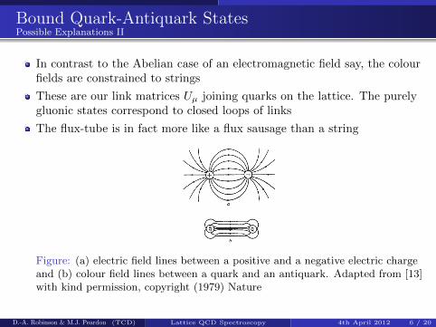
In contrast to the Abelian case of an electromagnetic field say, the colourfields are constrained to strings

These are our link matrices Uµ joining quarks on the lattice. The purelygluonic states correspond to closed loops of links

The flux-tube is in fact more like a flux sausage than a string

Figure: (a) electric field lines between a positive and a negative electric chargeand (b) colour field lines between a quark and an antiquark. Adapted from [13]with kind permission, copyright (1979) Nature


Bound Quark-Antiquark StatesPossible Explanations III

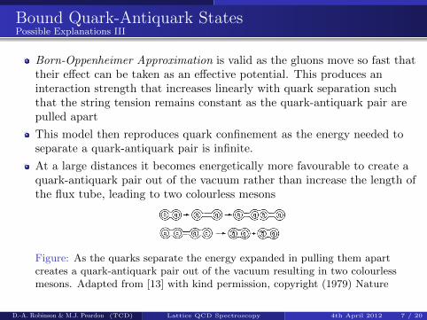
Born-Oppenheimer Approximation is valid as the gluons move so fast thattheir effect can be taken as an effective potential. This produces aninteraction strength that increases linearly with quark separation suchthat the string tension remains constant as the quark-antiquark pair arepulled apart

Model then reproduces quark confinement as the energy needed toseparate a quark-antiquark pair is infinite.

At a large distances it becomes energetically more favourable to create aquark-antiquark pair out of the vacuum rather than increase the length ofthe flux tube


Bound Quark-Antiquark StatesPossible Explanations III

Born-Oppenheimer Approximation is valid as the gluons move so fast thattheir effect can be taken as an effective potential. This produces aninteraction strength that increases linearly with quark separation suchthat the string tension remains constant as the quark-antiquark pair arepulled apart

This model then reproduces quark confinement as the energy needed toseparate a quark-antiquark pair is infinite.

At a large distances it becomes energetically more favourable to create aquark-antiquark pair out of the vacuum rather than increase the length ofthe flux tube, leading to two colourless mesons

Figure: As the quarks separate the energy expanded in pulling them apartcreates a quark-antiquark pair out of the vacuum resulting in two colourlessmesons. Adapted from [13] with kind permission, copyright (1979) Nature


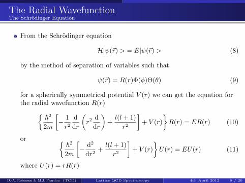
The Radial WavefunctionThe Schrodinger Equation

From the Schrodinger equation

H|ψ(~r) > = E|ψ(~r) > (8)

by the method of separation of variables such that

ψ(~r) = R(r)Φ(φ)Θ(θ) (9)

for a spherically symmetrical potential V (r) we can get the equation forthe radial wavefunction R(r){

~2

2m

[− 1

r2d

dr

(r2

d

dr

)+l(l + 1)

r2

]+ V (r)

}R(r) = ER(r) (10)

or {~2

2m

[− d2

dr2+l(l + 1)

r2

]+ V (r)

}U(r) = EU(r) (11)

where U(r) = rR(r)


The Radial WavefunctionThe Cornell Potential

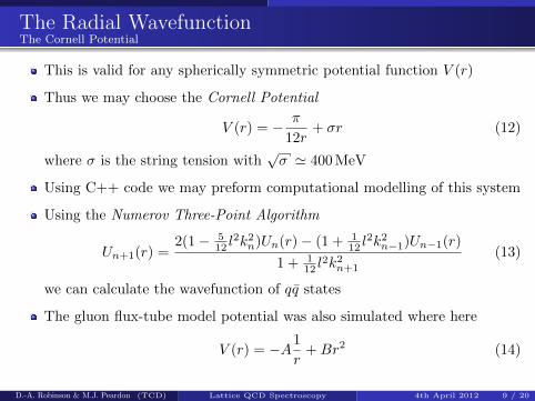
This is valid for any spherically symmetric potential function V (r)

Thus we may choose the Cornell Potential

V (r) = − π

12r+ σr (12)

where σ is the string tension with√σ ' 400 MeV

Using C++ code we may preform computational modelling of this system

Using the Numerov Three-Point Algorithm

Un+1(r) =2(1− 5

12 l2k2n)Un(r)− (1 + 1

12 l2k2n−1)Un−1(r)

1 + 112 l

2k2n+1

(13)

we can calculate the wavefunction of qq states

The gluon flux-tube model potential was also simulated where here

V (r) = −A1

r+Br2 (14)


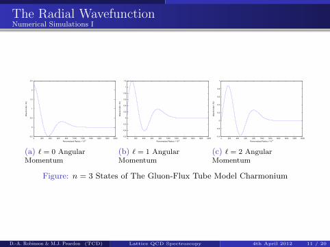
The Radial WavefunctionNumerical Simulations I

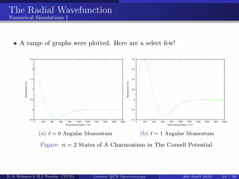
A range of graphs were plotted. Here are a select few!

-0.5

0

0.5

1

1.5

2

2.5

0 200 400 600 800 1000 1200 1400 1600 1800 2000

Wa

ve

fun

ctio

n,

R(r

)

Renormalised Radius, r*10-3

(a) ` = 0 Angular Momentum

-0.4

-0.2

0

0.2

0.4

0.6

0.8

0 200 400 600 800 1000 1200 1400 1600 1800 2000

Wa

ve

fun

ctio

n,

R(r

)


(b) ` = 1 Angular Momentum

Figure: n = 2 States of A Charmonium in The Cornell Potential


The Radial WavefunctionNumerical Simulations I

-0.5

0

0.5

1

1.5

2

2.5

0 200 400 600 800 1000 1200 1400 1600 1800 2000

Wa

ve

fun

ctio

n,

R(r

)


(a) ` = 0 AngularMomentum

-0.6

-0.4

-0.2

0

0.2

0.4

0.6

0.8

1

1.2

0 200 400 600 800 1000 1200 1400 1600 1800 2000

Wa

ve

fun

ctio

n,

R(r

)


(b) ` = 1 AngularMomentum

-0.4

-0.2

0

0.2

0.4

0.6

0.8

1

0 200 400 600 800 1000 1200 1400 1600 1800 2000

Wa

ve

fun

ctio

n,

R(r

)


(c) ` = 2 AngularMomentum

Figure: n = 3 States of The Gluon-Flux Tube Model Charmonium


The Radial WavefunctionNumerical Simulations III

Can also try to reproduce the qq specturm using the Cornell potential

0.4

0.6

0.8

1

1.2

1.4

1.6

1.8

2

2.2

2.4

2.6

S-Wave States P-Wave States D-Wave States F-Wave States

En

erg

y,

E

Figure: Charmonium Excitation States In The Cornell Potential


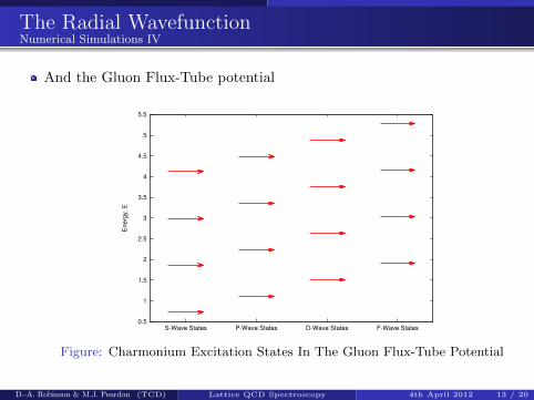
The Radial WavefunctionNumerical Simulations IV

And the Gluon Flux-Tube potential

0.5

1

1.5

2

2.5

3

3.5

4

4.5

5

5.5

S-Wave States P-Wave States D-Wave States F-Wave States

En

erg

y,

E

Figure: Charmonium Excitation States In The Gluon Flux-Tube Potential


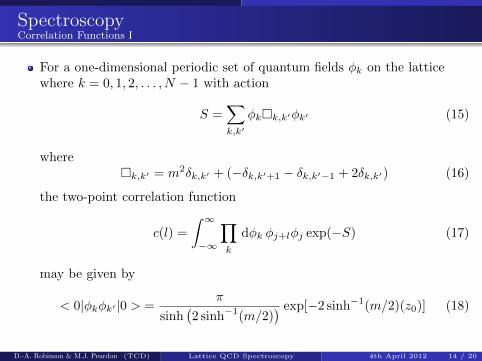
SpectroscopyCorrelation Functions I

For a one-dimensional periodic set of quantum fields φk on the latticewhere k = 0, 1, 2, . . . , N − 1 with action

S =∑k,k′

φk�k,k′φk′ (15)

where�k,k′ = m2δk,k′ + (−δk,k′+1 − δk,k′−1 + 2δk,k′) (16)

the two-point correlation function

c(l) =

∫ ∞−∞

∏k

dφk φj+lφj exp(−S) (17)

may be given by

< 0|φkφk′ |0 > =π

sinh(2 sinh−1(m/2)

) exp[−2 sinh−1(m/2)(z0)] (18)


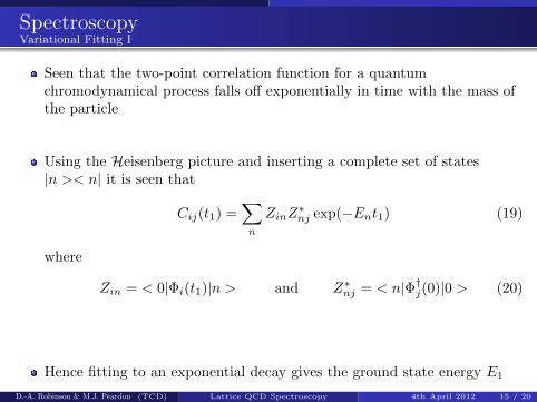
SpectroscopyVariational Fitting I

Seen that the two-point correlation function for a quantumchromodynamical process falls off exponentially in time with the mass ofthe particle

Using the Heisenberg picture and inserting a complete set of states|n >< n| it is seen that

Cij(t1) =∑n

ZinZ∗nj exp(−Ent1) (19)

where

Zin = < 0|Φi(t1)|n > and Z∗nj = < n|Φ†j(0)|0 > (20)

Hence fitting to an exponential decay gives the ground state energy E1


SpectroscopyVariational Fitting II

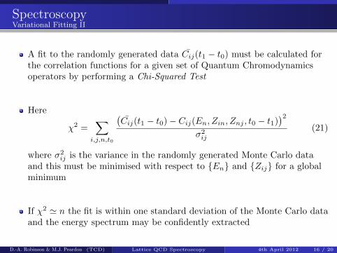
A fit to the randomly generated data Cij(t1 − t0) must be calculated forthe correlation functions for a given set of Quantum Chromodynamicsoperators by performing a Chi-Squared Test

Here

χ2 =∑

i,j,n,t0

(Cij(t1 − t0)− Cij(En, Zin, Znj , t0 − t1)

)2σ2ij

(21)

where σ2ij is the variance in the randomly generated Monte Carlo data

and this must be minimised with respect to {En} and {Zij} for a globalminimum

If χ2 ' n the fit is within one standard deviation of the Monte Carlo dataand the energy spectrum may be confidently extracted


SpectroscopyResults

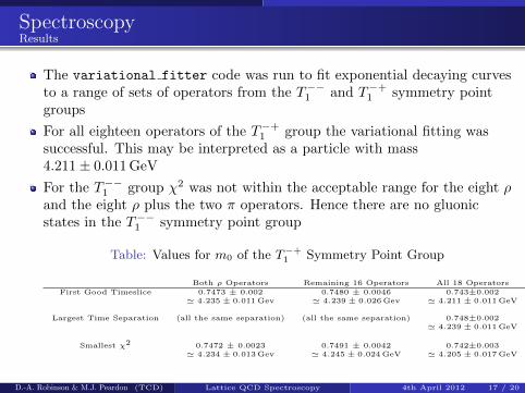
The variational fitter code was run to fit exponential decaying curvesto a range of sets of operators from the T−−1 and T−+1 symmetry pointgroups

For all eighteen operators of the T−+1 group the variational fitting wassuccessful. This may be interpreted as a particle with mass4.211± 0.011 GeV

For the T−−1 group χ2 was not within the acceptable range for the eight ρand the eight ρ plus the two π operators. Hence there are no gluonicstates in the T−−1 symmetry point group

Table: Values for m0 of the T−+1 Symmetry Point Group

Both ρ Operators Remaining 16 Operators All 18 Operators

First Good Timeslice 0.7473 ± 0.002 0.7480 ± 0.0046 0.743±0.002' 4.235 ± 0.011 Gev ' 4.239 ± 0.026 Gev ' 4.211 ± 0.011 GeV

Largest Time Separation (all the same separation) (all the same separation) 0.748±0.002' 4.239 ± 0.011 GeV

Smallest χ2 0.7472 ± 0.0023 0.7491 ± 0.0042 0.742±0.003' 4.234 ± 0.013 Gev ' 4.245 ± 0.024 GeV ' 4.205 ± 0.017 GeV


ConclusionsNumerical Simulations of the Radial Wavefunction

Can calculate the radial wavefunctions using numerical methods

The Cornell Potential and the gluon-flux tube potential may be used toreproduce the linear interaction term causing the wavefunctions to dropoff quickly with increasing r

Representative of the confinement property of Quantum Chromodynamics


ConclusionsLattice Quantum Chromodynamics Spectroscopy

Analytic calculation of correlation functions is complicated to begin with

Putting a quantum field theory on a lattice then introduces newcomplications

Still possible to compute such functions analytically using the Fouriertransform representation and the Green function method with the CauchyResidue Theorem

Find that the two-point correlation functions decay exponentially inEuclidean time with the mass of the state

Using variational fitting for the T−+1 group a physical states with mass of4.211± 0.011 GeV was found corresponding to an exotic cc state and thisis exactly where experiments at Belle and BABAR find states


ConclusionsFuture Work

Quantum Chromodynamics is an extremely interesting theory with ahuge number of research opportunities to offer

Accurately reproducing the charmonium spectrum will require furtherfine tuning and optimisation of the code

Extraction of the mass parameters of more states offers an increasingnumber of exotic states to be identified as physical states of the cc system

Remains to use the variational fitter code to fit the data generatedusing the CUDA LQCD Correlator Calculator software recentlydeveloped by O Conbhuı. This software is capable of calculating thecorrelation functions of quantum fields in an extremely computationallyinexpensive fashion with the prospect of predicting new mesonic states


References

H. Fritzsch, M. Gell-Mann and H. Leutwyler, Physics Letters 47 B, 365 (1973).

C. N. Yang and R. L. Mills, Physical Review 96, 191 (1954).

M. Gell-Mann, Physics Letters 8, 214 (1964).

G. Zweig, CERN Rep. 8182/TH.401, 8419/TH.412.

O. W. Greenberg, Physical Review Letters 13, 589 (1964).

O. W. Greenberg and C. A. Nelson, Physics Reports 32C, 69 (1977).

O. W. Greenberg, American Journal of Physics 50, 1074 (1982).

K. G. Wilson, Physical Review D 10, 2445 (1974).

R. P. Feynman, Review of Modern Physics 20, 367 (1948).

D. H. Perkins, Introduction to High-Energy Physics (Addison-Wesley, Massachusetts) 99 (1982).

A. Chodos, R. L. Jaffe, K. Johnson, C. B. Thorn and V. F. Weisskopf, Physical Review D 9, 3471 (1974).

P. Hasenfratz and J. Kuti, Physics Reports 40 C, 75 (1978).

W. Marciano and H. Pagels, Nature 279, 497 (1979).

P. O Conbhuı and M. J. Peardon, Computing Two-Point Correlator Functions On Graphics Processor Units

(2012).


Thank youAny Questions???

Any Questions???

AcknowledgementsDr. Mike J. Peardon†

Sr. Pol Vilaseca Marinar‡, Mr. Graham Moir§ and Mr. Tim Harris Sch.§

Mr. Padraig O Conbhuı¶ and Mr. Cian Booth¶

And all of the Lattice Quantum Chromodynamics undergraduate students.


SpectroscopyCorrelation Functions I

For a one-dimensional periodic set of quantum fields φk on the latticewhere k = 0, 1, 2, . . . , N − 1 with action

S =∑k,k′

φk�k,k′φk′ (22)

where�k,k′ = m2δk,k′ + (−δk,k′+1 − δk,k′−1 + 2δk,k′) (23)

the two-point correlation function

c(l) =

∫ ∞−∞

∏k

dφk φj+lφj exp(−S) (24)

may be given by

c(l) =1

Z[0]

∂

∂Jj+l

∂

∂jZ[J ]

∣∣∣∣J=0

(25)

where Z0[J ] is the generating functional, with J a source field, given by

Z0[J ] =

∫ ∞−∞

d[φ(x)] exp

(−S[φ(x)] +

∫ ∞−∞

J(x)φ(x)

)(26)


SpectroscopyCorrelation Functions II

Writing S as a matrix M and performing a Gaussian integration we findthat

c(l) =

√π

det(M)

1

4M−1j+l,j (27)

It remains to find the eigenvalues, and thus the inverse matrix elementsM−1k,k′

Reverting to four-space and using the Fourier transform representation

Mk,k′ =

∫ ∞−∞

d4p

(2π)4M(p) exp[ip(k − k′)] (28)

where

M(p) =

∫ ∞−∞

M(k) exp(−ipk)dk (29)

=1

(2π)4(m2 + 4 sin2(p/2)

)(30)


SpectroscopyCorrelation Functions III

And a Green function to calculate the inverse matrix

M−1k,k′ =

∫ ∞−∞

d4p

(2π)4G(k) exp[ip(k − k′)] (31)

such that�G(k) = δ(k) (32)

yielding

G(k) = (2π)41

m2 + 4 sin2(p/2)(33)


SpectroscopyCorrelation Functions IV

And the Cauchy Residue Theorem∫γ

f(z)dz = 2πi∑j

n(wj , γ)Resz=wjf(z)

with Resz=wjf(z) = limz→wj

(z − wj) f(z) =g(wj)

h′(wj)(34)

to evaluate, with z = k − k′ for ease, the complex integral

M−1k,k′ =

∫ ∞−∞

d3~p exp(−i~p · ~z)∫ ∞−∞

dp01

m2 + 4 sin2(p/2)exp(ip0z0) (35)

we find that

< 0|φkφk′ |0 > = M−1k,k′ =π

sinh(2 sinh−1(m/2)

) exp[−2 sinh−1(m/2)(z0)]

(36)


Documents

Lattice Quantum Chromodynamics Spectroscopyrobinson/labs/lqcd_presentation_handout.pdf · Lattice Quantum Chromodynamics Spectroscopy |{Monte Carlo Searches For Exotic Charmonium