Lattice Mechanics of Origami Tessellations

Arthur A. Evans1, Jesse L. Silverberg2, and Christian D. Santangelo1

1 Department of Physics, UMass Amherst, Amherst MA 01003, USA and2 Department of Physics, Cornell University, Ithaca, NY 14853, USA

Origami-based design holds promise for developing materials whose mechanical properties aretuned by crease patterns introduced to thin sheets. Although there has been heuristic developmentsin constructing patterns with desirable qualities, the bridge between origami and physics has yet tobe fully developed. To truly consider origami structures as a class of materials, methods akin tosolid mechanics need to be developed to understand their long-wavelength behavior. We introducehere a lattice theory for examining the mechanics of origami tessellations in terms of the topology oftheir crease pattern and the relationship between the folds at each vertex. This formulation providesa general method for associating mechanical properties with periodic folded structures, and allowsfor a concrete connection between more conventional materials and the mechanical metamaterialsconstructed using origami-based design.

While for hundreds of years origami has existed as anartistic endeavor, recent decades have seen the applica-tion of folding thin materials to the fields of architecture,engineering, and material science [1–7]. Controlled ac-tuation of thin materials via patterned folds has led toa variety of self-assembly strategies in polymer gels [8]and shape-memory materials [4], as well elastocapillaryself-assembly [9], leading to the design of a new categoryof shape-transformable materials inspired by origami de-sign. The origami repertoire itself, buoyed by advancesin the mathematics of folding and the burgeoning fieldof computational geometry [10], is no longer limited todesigns of animals and children’s toys that dominate theart in popular consciousness, but now includes tessella-tions, corrugations, and other non-representational struc-tures whose mechanical properties are of interest from ascientific perspective. These properties originate fromthe confluence of geometry and mechanical constraintsthat are an intrinsic part of origami, and ultimately allowfor the construction of mechanical meta-materials usingorigami-based design [1–4, 6, 11–13]. In this paper weformulate a general theory for periodic lattices of folds inthin materials, and combine the language of traditionallattice solid mechanics with the geometric theory under-lying origami.

A distinct characteristic of all thin materials is thatgeometric constraints dominate the mechanical responseof the structure. Because of this strong coupling betweenshape and mechanics, it is far more likely for a thin sheetto deform by bending without stretching. Strategicallyweakening a material with a crease or fold, and thus low-ering the energetic cost of stretching, allows complex de-formations and re-ordering of the material for negligibleelastic energy cost. This vanishing energy cost, espe-cially combined with increased control over micro- andnanoscopic material systems, indicates the great promisefor structures whose characteristics depend primarily ongeometry, rather than material composition.

By patterning creases, hinges, or folds into an other-wise flat sheet (be it composed of paper, metal or poly-mer gel), the bulk material is imbued with an effectivemechanical response. In contrast to conventional com-

posites engineering, wherein methods generally rely ondesigning response based on the interaction between theconstituent parts that compose the material, origami-based design injects novelty at the “atomic” level; evensingle vertices of origami behave as engineering mech-anisms [14], providing novel functionality such as com-plicated bistability [15–17] and auxetic behavior [6, 11–13]. This generic property inspires the identification oforigami tessellations with mechanical metamaterials, or acomposite whose effective properties arise from the struc-ture of the unit cell. Although originally introduced toguide electromagnetic waves[18], rationally designed me-chanical metamaterials have since been developed thatcontrol wave propagation in acoustic media [19, 20], thinelastic sheets and curved shells[21–24], and harness elas-tic instabilities to generate auxetic behavior [25–29].

Traditional metamaterials invoke the theory of lin-ear response in wave systems, but currently there is nogeneral theory for predicting the properties of origami-inspired designs on the basis of symmetry and structure.In the following we propose a general framework for an-alyzing the kinematics and mechanics of an origami tes-sellation as a crystalline material. By treating a periodiccrease pattern, we naturally connect the geometric math-ematics of origami to the more conventional analysis ofelasticity in solid state lattice structures. In section I weoutline the general formalism required to find the kine-matic solutions for a single origami vertex. In section IIwe discuss the general formulation for a periodic lattice,including both the kinematics of deformation modes andenergetics for a periodic crease pattern. In section IIIwe examine the well-known case study of the Miura-oripattern. Our analysis here recovers known aspects of theMiura-ori pattern as well as identifies key features thathave not been quantitatively discussed previously.

I. SINGLE ORIGAMI VERTEX

Many of the design strategies for self-folding materialsinvolves a single fold, an array of non-intersecting folds,or an array of folds that intersect only at the boundary

arX

iv:1

503.

0575

6v2

[co

nd-m

at.s

oft]

9 J

ul 2

015

2

Block@8a = p ê 3<,ContourPlot3D@EnergyLandscape@a, fp, fm, e, p ê 2, p ê 2 - 0.3, 2.7, 5, .1D,8fp, p, 2 p - 0.001<, 8fm, p, 2 p - 0.001<, 8e, 0, 2 p<,BaseStyle Ø 8FontSize Ø 18<, ColorFunction Ø "Autumn",PlotLegends Ø BarLegend@Automatic, All, LabelStyle Ø 8FontSize Ø 18<D,Contours Ø 8Automatic, 50<DD

$Aborted

H*Need Tessellatica to do this part*L

In[2060]:= sectorangles = 880 °, 70. °, 30. °, 60. °, 90 °, 30. °<;8gm2, gm6< = 880. °, 40. °<;vtobj = MakeYoshimuraVertex@sectorangles, 8gm2, gm6<D;

Show@Vertex3DFoldedFormGraphics3D@vtobj, DihedralAngleLabels ØHStyle@Ò, Italic, 26D & êü 8"f1" , "f2", "f3", "f4" , "f5", "f6"<L,

SectorAngleLabels Ø HStyle@Ò, Italic, 26D & êü 8"a1", "a2", "a3", "a4" , "a5", "a6"<L,RealSphereRadius Ø 0.5D ê. OrigamiStyle@WhiteSideColor Ø GreenDD

Out[2063]=

GeneralMSV.nb 9

b)

↵1↵2

↵3

↵4

↵5↵6

f1

f2

f3

f4

f5

f6

a) c)

↵2

↵3

↵4

↵5

f1

f2

f3

f4

f5

f6 `2

`3

`4

`1 = ↵1`5 = ↵6

A B C

FIG. 1. (color online) (A) Graph for a single vertex. This degree six vertex has its graph determined by the six sector anglesαi. Each crease has a dihedral angle fi associated with it. In the flat case every fi = π, or equivalently, every fold angle isidentically zero, since the fold angle is defined as the supplement of the dihedral angle. (B) By assigning fold angles to eachcrease, a 3D embedding of the vertex (i.e. the folded form of the origami) is fully determined. Every face must rotate rigidlyabout the defined creases, and the sector angles must remain constant. There is a limited set of fold angles that will solve theseconditions. (C) Schematic projection of the curve of intersection between the unit sphere and the folded form origami. For anN -degree vertex this projection generates a spherical N -gon. To proceed, the N -gon is divided into N -2 spherical triangles andthe interior angles (i.e. the fi) follow as a result of applying the rules of spherical trigonometry. All three dimensional origamistructures are visualized using Tessellatica, a freely available online package for Mathematica [30].

of the material [9, 31–34]. From a formal standpoint, wedefine a fold as a straight line demarcating the bound-ary between two flat sheets of unbendable, unstretchablematerial. These sheets, in isolation, are allowed to ro-tate around the fold, so that the structure behaves me-chanically like a simple hinge. If the fold is producedby plastically deforming a piece of material, rather thanfunctioning as a hinge the fold has a preferred angle, andis more precisely called a crease. Herein we shall use theterms interchangeably, since the kinematic motions of afold and the energetics involved for a crease can be de-scribed separately. An important, and arguably defining,characteristic of an origami structure is that it requiresthat more than one fold meet at a vertex. While each foldindividually allows for unrestricted rigid body rotation ofa sheet, geometrical constraints arise when several foldscoincide at a vertex. These constraints are what provideorigami structures with their mechanical novelty, and ul-timately are why deployable structures and mechanicalmetamaterials display exotic and tunable properties.

A vertex of degree N is defined as a point where Nstraight creases meet. Figure 1A shows the crease pat-tern for a schematic 6-degree vertex, with sectors definedby planar angles αi. The three-dimensional folded formof this vertex is found by supplying fold angles to each ofthe creases, subject to the constraints mentioned previ-ously [35, 36]. This procedure is an exercise in sphericaltrigonometry.

One way to visualize the constraints is to surroundeach vertex with a sphere and consider the intersectionbetween it and the surface (Fig. 1B). In this construction,the side lengths of the spherical polygon are the angles

between adjacent folds, which must remain fixed, andthe dihedral fold angles are the internal angles of thepolygon on the sphere. Since an N -sided polygon hasN −3 continuous degrees of freedom, each vertex does aswell. These N − 3 degrees of freedom can be thought of,for example, as the angles between a fixed fold and theremaining non-adjacent folds.

Starting with a general vertex containing dihedral an-gles fi, we use spherical trigonometry to calculate theseangles in terms of the N -3 degrees of freedom. To calcu-late f1 we partition the angle into sectors by subdivid-ing the spherical N -gon into N − 2 triangles (Fig. 1C).We label the angles that lead from f1 to fi as `i, where`1 = α1 and `N−1 = αN are sector angles. All the anglesαi are spherical polygon edges, and since origami struc-tures allow only isometric deformations, these angles areconstant. The `i are the angles subtended by drawing ageodesic on the encapsulating sphere from f1 to fi; ex-pressions for relating the `i to the fold angles fi are foundby using the spherical law of cosines around the vertex[35]:

3

f1 =

N−2∑i=1

cos−1

[cosαi+1 − cos `i+1 cos `i

sin `i+1 sin `i

], (1)

f2 = cos−1

[cos `2 − cosα1 cosα2

sinα1 sinα2

], (2)

fN = cos−1

[cos `N−2 − cosαN−1 cosαN

sinαN−1 sinαN

], (3)

fi = cos−1

[cos `i−2 − cosαi−1 cos `i−1

sin `i−1 sinαi−1

]+ (4)

cos−1

[cos `i − cosαi cos `i−1

sin `i−1 sinαi

].

These expressions are essentially all that is requiredto determine the folding of a single vertex, although theassociated solutions are generically multi-valued. Theseresults imply that there are multiple branches of config-uration space for any given spherical polygon.

To specify the internal state of each vertex we definean N−3 component vector s. Given the internal state ofa vertex, all N of the dihedral fold angles are determined,which we collect in the vector f(s). In practice, compu-tations are vastly simplified by choosing the appropriatedegrees of freedom; for example, for a degree 6 vertex ofthe type displayed in Fig. 1, we choose s = {`3, f2, f6},and the fold vector is given by f = {f1, f2, f3, f4, f5, f6}.

II. GENERAL LATTICE THEORY

To determine the mechanical properties of an origamitessellation we begin by examining how many verticesare connected together in a crease pattern. When con-structing a real piece of origami, artists and designersspecify “mountain” and “valley” creases in the patternto encode instructions for how the structure will fold. Inour formulation we will treat the crease pattern as a sim-ple connected graph, where each unique crease is an edgethat connects two vertices to one another.

A. Kinematically allowed deformations

In addition to the origami constraints discussed abovefor a single vertex, joining multiple vertices together gen-erates further constraints on the folds. Consider a creasepattern that consists of P vertices. Each vertex vp,with p ∈ {1, ..., P} has Np folds, collected in the vec-tor fp = (fp1 f

p2 · · · f

pNp

)T . If we collect all the folds into

the vector F , given by

f11

f12

f13

f14

f24

f23

f22

f21

f11

f12

f13

f14 f2

4

f23

f22

f21

a) b)A B

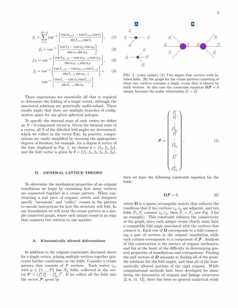
FIG. 2. (color online) (A) Two degree four vertices with la-beled folds. (B) the graph for the crease pattern consisting ofthese two vertices contains a single crease that is shared byboth vertices. In this case the constraint equation DF = 0simply becomes the scalar relationship f1

1 = f23 .

F =

f11

f12...f1N1

f21...f2N2

...fP1...

fPNP

, (5)

then we have the following constraint equation for thefolds:

DF = 0, (6)

where D is a sparse rectangular matrix that enforces thecondition that if two vertices vq, vp are adjacent, and twofolds Fi,Fj connect vq, vp, then Fi = Fj (see Fig. 2 foran example). This constraint enforces the connectivityof the graph, since each unique crease clearly must havea compatible fold angle associated with the vertices thatconnect it. Each row of D corresponds to a fold connect-ing a pair of vertices in the origami tessellation whileeach column corresponds to a component of F . Analysisof this construction is the essence of origami mechanics,and lies at the heart of the difficulty in determining gen-eral properties of tessellations and corrugations. Findingthe null vectors of D amounts to finding all of the possi-ble solutions for the fold angles, and thus all of the kine-matically allowed motions of the rigid origami. Whilecomputational methods have been developed for simu-lating the kinematics of origami and linkage structures[2, 6, 11, 12], there has been no general analytical study

4

that seeks to identify mechanical properties based solelyon the crease and fold patterns.

The functions F(s) are, in general, nonlinear. To pro-ceed analytically, we expand s about a state s0 that solvesthe constraint equations. That is, if F(s0) = F0 thenDF0 ≡ 0. A trivial choice for s0 has every entry iden-tically equal to π, indicating that the piece of origamiis unfolded. The more common, and more interesting,scenario involves a folded state where the values of theinternal vector s0 are known. Assuming that such a stateexists, we write s = s0 +δs, with δs a small perturbation,and then have

DJδs ≡ Rδs = 0, (7)

where the Jacobian of the fold angles for each vertexJ ≡ ∂F/∂s|s0 is a block diagonal matrix defining thesmall deviations from the “ground state” s0, and R is arigidity matrix that informs on the infinitesimal isomet-ric deformations of the origami structure [37, 38]. Thisformulation is convenient since it separates the effectsof the crease pattern topology (contained entirely in D)from the constrained motion of a single vertex (containedentirely in J). We can thus solve for each of these matri-ces individually.

To find D, we first exploit the periodicity of the latticeto decompose the vector F and matrix D in a Fourierbasis, such that F =

∑n,m e

iq·xFq + c.c.. Here q is atwo-dimensional wave-vector and x = na1 + ma2 is the2D position vector of the fundamental unit cell on thecrease pattern lattice, where (n,m) indexes this positionin terms of the lattice vectors a1,2. Since F ≈ Jδs andJ is independent of the lattice position, we also haveδs =

∑n,m e

iq·xδsq + c.c., where Fq = Jδsq. In thisrepresentation the constraints given in Eq. 6 are

D(q)Fq = D(q)Jδsq = 0 (8)

Now, instead of a matrix operation over all the ver-tices, the size of D(q) is vastly simplified. For a patternwith p distinct vertices per unit cell, each of degree Np,D(q) is a (

∑pi=1 (Ni/2)×

∑pi=1Ni) matrix. In Fourier

space, D(q) is the complex-valued constraint matrix forthe graph of the unit cell vertices and folds. Specifically,each fold of the unit cell is represented by a row in D(q)having only two nonzero entries. Those entries all havethe form ±eiq·a1 ,±eiq·a2 ,±1, depending on whether thefold connects to an adjacent unit cell along a1,2 or isinternal to the unit cell.

The formulation in terms of the matrix R(q) is com-pletely general for any origami tessellation. The rect-angular matrix D(q) carries all of the topological infor-mation regarding the fold network, while the Jacobian Jcarries the information about the type of vertex that hasbeen specified. J will be block diagonal with one blockfor each vertex of a unit cell, but does not depend on qfor a regular tessellation.

B. Origami energetics

While the R matrix determines the kinematically iso-metric deformation to leading order, these constraintsare generally not the end of the story for real materi-als. Creases in folded paper, thermoresponsive gels withprogrammed folding angles, and elastocapillary hingesall balance energetic considerations with geometric con-straints. In many cases these creases and hinges act astorsional springs, while the bending of faces have addi-tional elastic energy content [7, 39, 40].

The energy associated with the entire structure maybe written, to quadratic order in the dihedral vectors, as

E =1

2(F −F0)

T A (F −F0) , (9)

where A is a general stiffness matrix and F0 is a ref-erence fold angle. For linear response this is the mostgeneric form for the energy. In the simplest of cases Ais constant over the lattice and diagonal with respect toF ; this models each crease as a torsional spring withuniform spring constant [7, 13, 40]. Small amplitude re-sponse is found by examining the origami structure nearthe ground state, that is, when F = F0. When theenergy is expanded about the ground state E0 we find

E = E0 +1

2δsTJTAJδs, (10)

or in the Fourier decomposition,

E =LW

2

∑q

δs†qMδsq, (11)

where L is the length of the tessellation in the a1 direc-tion, W is the width in the a2 direction, andM = JTAJis a matrix operator that is independent of wavenumber.Since the nullspace of R(q) will determine the modes ofdeformation, the solution to this problem lies in findingthe kinematically allowed deformations, and then any en-ergetic description will simply involve a change of basisto a system of deformations that diagonalize the operatorM.

III. MIURA-ORI

As an example of this formulation, we consider inho-mogeneous deformations of a particular origami meta-material, the Miura-ori. First introduced as a frameworkfor a deployable surface, the design appears often in na-ture, from plant leaves [41] to animal viscera [42]. Ad-ditionally, theoretical calculations and experiments havesuggested the Miura-ori as a canonical, origami-based,auxetic metamaterial [6, 7, 11–13]. Its ubiquity maybe related to its simplicity: the Miura-ori is determined

5

A

✓+✓�

�+

��

�+

��

In[94]:= Graphics3DB::Green, Opacity@0.9D,Polygon@88O1, O3, O8, O9<, 8O2, O3, O8, O4<, 8O4, O5, O6, O8<, 8O9, O7, O6, O8<<D ê.

:a Ø 1, b Ø 1, g Øp

2- 0.3, q Ø

p

4>>, ,

:Blue, Opacity@0.3D, SphereB:TanA p

2- 0.3E CosA p

4E

1 + TanA p

2- 0.3E2 CosA p

4E2

, 1 - SinBp

2- 0.3F

2SinB

p

4F2

+

1 -TanA p

2- 0.3E CosA p

4E

1 + TanA p

2- 0.3E2 CosA p

4E2

2

, SinBp

2- 0.3F SinB

p

4F>, 0.4F>>, Boxed Ø FalseF

Out[94]=

In[34]:= Face1 = Graphics3D@Table@Polygon@8O1 + 82 S n, 2 L m, 0<, O3 + 82 S n, 2 L m, 0<,O8 + 82 S n, 2 L m, 0<, O9 + 82 S n, 2 L m, 0<<D, 8n, 0, 5, 1<, 8m, 0, 5, 1<DD;

Face2 = Graphics3D@Table@Polygon@8O2 + 82 S n, 2 L m, 0<, O3 + 82 S n, 2 L m, 0<,O8 + 82 S n, 2 L m, 0<, O4 + 82 S n, 2 L m, 0<<D, 8n, 0, 5, 1<, 8m, 0, 5, 1<DD;

Face3 = Graphics3D@Table@Polygon@8O4 + 82 S n, 2 L m, 0<, O8 + 82 S n, 2 L m, 0<,O6 + 82 S n, 2 L m, 0<, O5 + 82 S n, 2 L m, 0<<D, 8n, 0, 5, 1<, 8m, 0, 5, 1<DD;

Face4 = Graphics3D@Table@Polygon@8O9 + 82 S n, 2 L m, 0<, O8 + 82 S n, 2 L m, 0<,O6 + 82 S n, 2 L m, 0<, O7 + 82 S n, 2 L m, 0<<D, 8n, 0, 5, 1<, 8m, 0, 5, 1<DD;

MiuraPlot.nb 3

✏

✓+✓�

�+

��

�+

��

B

↵

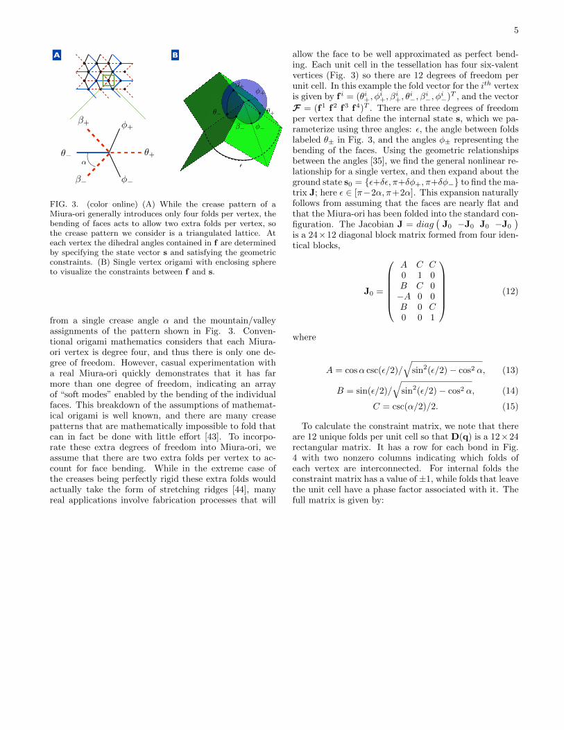
FIG. 3. (color online) (A) While the crease pattern of aMiura-ori generally introduces only four folds per vertex, thebending of faces acts to allow two extra folds per vertex, sothe crease pattern we consider is a triangulated lattice. Ateach vertex the dihedral angles contained in f are determinedby specifying the state vector s and satisfying the geometricconstraints. (B) Single vertex origami with enclosing sphereto visualize the constraints between f and s.

from a single crease angle α and the mountain/valleyassignments of the pattern shown in Fig. 3. Conven-tional origami mathematics considers that each Miura-ori vertex is degree four, and thus there is only one de-gree of freedom. However, casual experimentation witha real Miura-ori quickly demonstrates that it has farmore than one degree of freedom, indicating an arrayof “soft modes” enabled by the bending of the individualfaces. This breakdown of the assumptions of mathemat-ical origami is well known, and there are many creasepatterns that are mathematically impossible to fold thatcan in fact be done with little effort [43]. To incorpo-rate these extra degrees of freedom into Miura-ori, weassume that there are two extra folds per vertex to ac-count for face bending. While in the extreme case ofthe creases being perfectly rigid these extra folds wouldactually take the form of stretching ridges [44], manyreal applications involve fabrication processes that will

allow the face to be well approximated as perfect bend-ing. Each unit cell in the tessellation has four six-valentvertices (Fig. 3) so there are 12 degrees of freedom perunit cell. In this example the fold vector for the ith vertexis given by f i = (θi+, φ

i+, β

i+, θ

i−, β

i−, φ

i−)T , and the vector

F = (f1 f2 f3 f4)T . There are three degrees of freedomper vertex that define the internal state s, which we pa-rameterize using three angles: ε, the angle between foldslabeled θ± in Fig. 3, and the angles φ± representing thebending of the faces. Using the geometric relationshipsbetween the angles [35], we find the general nonlinear re-lationship for a single vertex, and then expand about theground state s0 = {ε+δε, π+δφ+, π+δφ−} to find the ma-trix J; here ε ∈ [π−2α, π+2α]. This expansion naturallyfollows from assuming that the faces are nearly flat andthat the Miura-ori has been folded into the standard con-figuration. The Jacobian J = diag

(J0 −J0 J0 −J0

)is a 24×12 diagonal block matrix formed from four iden-tical blocks,

J0 =

A C C0 1 0B C 0−A 0 0B 0 C0 0 1

(12)

where

A = cosα csc(ε/2)/

√sin2(ε/2)− cos2 α, (13)

B = sin(ε/2)/

√sin2(ε/2)− cos2 α, (14)

C = csc(α/2)/2. (15)

To calculate the constraint matrix, we note that thereare 12 unique folds per unit cell so that D(q) is a 12×24rectangular matrix. It has a row for each bond in Fig.4 with two nonzero columns indicating which folds ofeach vertex are interconnected. For internal folds theconstraint matrix has a value of ±1, while folds that leavethe unit cell have a phase factor associated with it. Thefull matrix is given by:

6

x

y

123

45

67

89

1011

12

161718

1314 15

222324

1920 21

a

b

A B

C ei(qxa/2+qyb/2)

8

14

3

151322

ei(qxa/2) ei(qyb/2)

FIG. 4. (color online) (A) Miura-ori, without the assignment of mountain/valley folds, has a simple directed graph structurewith a unit cell composed of four vertices. By tessellating these four vertices the entire pattern emerges. Note that thetessellation is rectangular, with lattice vectors a1 = ax and a2 = by. (B) Each vertex has six folds, labelled in the fashionshown here. (C) In Fourier space, translations associated with connecting these folds together throughout the tessellationmerely amounts to a phase factor associated with the appropriate wave number and lattice vector. Left: Translating in the xdirection. Middle: Translating in the y direction. Right: Connecting the extra folds involves a diagonal translation across theunit cell. Note that the five internal folds have a phase factor identically equal to one.

7

DT (q) =

1 0 0 0 0 0 0 0 0 0 0 0

0 eiqy2 0 0 0 0 0 0 0 0 0 0

0 0 eiqy2 0 0 0 0 0 0 0 0 0

0 0 0 −e−iqx2 0 0 0 0 0 0 0 0

0 0 0 0 −1 0 0 0 0 0 0 00 0 0 0 0 −1 0 0 0 0 0 0

0 0 0 eiqx2 0 0 0 0 0 0 0 0

0 0 0 0 0 0 eiqx2 +

iqy2 0 0 0 0 0

0 0 0 0 0 0 0 eiqy2 0 0 0 0

−1 0 0 0 0 0 0 0 0 0 0 00 0 0 0 0 0 0 0 −1 0 0 0

0 0 0 0 0 0 0 0 0 eiq2 0 0

0 0 0 0 0 0 0 0 0 0 −e−iq2 0

0 0 0 0 0 0 −e−iqx2 −

iqy2 0 0 0 0 0

0 0 −e−iqy2 0 0 0 0 0 0 0 0 0

0 0 0 0 0 0 0 0 0 0 0 10 0 0 0 1 0 0 0 0 0 0 0

0 0 0 0 0 0 0 0 0 −e−iqx2 0 0

0 0 0 0 0 0 0 0 0 0 0 −1

0 −e−iqy2 0 0 0 0 0 0 0 0 0 0

0 0 0 0 0 0 0 −e−iqy2 0 0 0 0

0 0 0 0 0 0 0 0 0 0 eiqx2 0

0 0 0 0 0 0 0 0 1 0 0 00 0 0 0 0 1 0 0 0 0 0 0

(16)

A. Bulk deformation

The combination D(q)J is square such that Eq. (7) hasa nontrivial solution whenever det [D(q)J] = 0. We non-dimensionalize the wavenumber by the physical lengthsof the lattice vectors such that qx → qxa and qy → qyb,and the resulting dispersion relation is

cos2 α

sin4(ε0/2)sin2(qx/2) + sin2(qy/2) = 0. (17)

The only real solution to this equation is q = 0, indi-cating that an infinite origami tessellation does not admitspatially inhomogeneous solutions; only uniform defor-mations are allowed. The nullspace of R is three dimen-sional here, corresponding to three uniform deformationmodes of the Miura-ori. These zero modes are given bythe vectors Ψi:

ΨI =

100100100100

, ΨII =

0−110−110−110−11

, ΨIII =

−2CA11011−2CA

11011

(18)

These infinitesimal deformations of the unit cell corre-spond to a uniform contraction, a twisting mode, and asaddle-like deformation, respectively (see Fig. 5).

To describe the kinematics of deformation, all we re-quire are the null vectors of the constraint equations, butfor examining energy associated with the creases we needto calculate the eigenvalues of the matrixM = JTAJ. Ingeneral, it is not unreasonable to assume that a creasedand folded Miura-ori will have a crease stiffness k thatis approximately equal for all patterned creases, but theenergy scale for bending of the faces will depend on the

8

I

II

III

�

�

I

II

III

In[1876]:= faspecs = MakeStdFoldAngleSpecs@tobj1Dfoldangles = MakeGraphFoldAngles@tobj1, faspecsD;tobjff1 = FoldGraph3D@tobj1, foldanglesD;groundstate = FoldedFormGraphics3D@tobjff1D ê.

OrigamiStyle@Opacity3D Ø 1, WhiteSideColor Ø Darker@RedD, ColoredSideColor Ø PinkDOut[1876]= 88¶, 0<, 8¶, 0<, 81, -90 °<, 81, 90 °<, 8¶, 0<, 8¶, 0<, 8¶, 0<, 81, -90 °<,

8¶, 0<, 8¶, 0<, 81, -90 °<, 8¶, 0<, 81, 0<, 81, 0<, 81, 0<, 81, 0<<

Out[1879]=

ArtTessellationSimulation.nb 7

In[1866]:= tobjff1 = FoldGraph3D@tobj1, foldanglesD;twist = FoldedFormGraphics3D@tobjff1D ê.

OrigamiStyle@Opacity3D Ø 1, WhiteSideColor Ø Darker@RedD, ColoredSideColor Ø PinkD

Out[1867]=

ShowBFoldedFormGraphics3D@tobjff1D ê. OrigamiStyle@D,

Graphics3DB:Blue, Opacity@0.3D, SphereB:1, 3 í 2, 0>, 0.45F>FF

10 ArtTessellationSimulation.nb

In[1872]:= faspecs = 88¶, 0<, 8¶, 0<, 81, -90 °<, 81, 90 °<, 8¶, 0<, 8¶, 0<, 8¶, 0<, 81, -90 °<,8¶, 0<, 8¶, 0<, 81, -90 °<, 8¶, 0<, 810, p ê 6<, 810, p ê 6<, 810, p ê 6<, 810, p ê 6<<

foldangles = MakeGraphFoldAngles@tobj1, faspecsD;tobjff1 = FoldGraph3D@tobj1, foldanglesD;saddle = FoldedFormGraphics3D@tobjff1D ê.

OrigamiStyle@Opacity3D Ø 1, WhiteSideColor Ø Darker@RedD, ColoredSideColor Ø PinkD

Out[1872]= :8¶, 0<, 8¶, 0<, 81, -90 °<, 81, 90 °<, 8¶, 0<, 8¶, 0<, 8¶, 0<, 81, -90 °<,

8¶, 0<, 8¶, 0<, 81, -90 °<, 8¶, 0<, :10,p

6>, :10,

p

6>, :10,

p

6>, :10,

p

6>>

Out[1875]=

ArtTessellationSimulation.nb 11

BA

In[3151]:= LogLogPlotB:8, 1 + G,2 H3 + GL

3>, 8G, 0.001, 1000<,

Ticks Ø 88.01, .1, 1, 10, 100<, 80.001, .01, .1, 1, 10, 100, 1000<<,PlotRange Ø 880.001, 1000<, 80.001, 1000<<,

PlotStyle Ø 88Thick, Black<, 8Thick, Red<, 8Thick, Blue<<, BaseStyle Ø FontSize Ø 18F

Out[3151]=

0.01 0.1 1 10 1000.001

0.01

0.1

1

10

100

1000

In[2649]:= EigenvectorsB

2.1281952649600777` 0 -1.1558764934449623`

0 G + 14CscB

9 p

40F2

0.`

-1.1558764934449626` 0 1.6869850761862608` + 0.05512637537771714` G

F

EigenvaluesB

2.1281952649600777` 0 -1.1558764934449623`

0 G + 14CscB

9 p

40F2

0.`

-1.1558764934449626` 0 1.6869850761862608` + 0.05512637537771714`

F

Out[2649]= ::-0.190855 + 0.0238461 G + 0.432572 5.53887 - 0.0486446 G + 0.00303892 G2 , 0., 1.>,

:-0.190855 + 0.0238461 G - 0.432572 5.53887 - 0.0486446 G + 0.00303892 G2 , 0., 1.>,

80., 1., 0.<>

Out[2650]= :0.5 3.81518 + 0.0551264 G - 5.53887 - 0.0486446 G + 0.00303892 G2 ,

0.5 3.81518 + 0.0551264 G + 5.53887 - 0.0486446 G + 0.00303892 G2 , G +1

4CscB

9 p

40F2>

In[2654]:= SeriesB::-0.19085524763066966` + 0.023846135677272513` G + 0.4325721673859852`

5.5388683030723165` - 0.048644636973637745` G + 0.003038917262284979` G2 ,

0.`, 1.`>, :-0.19085524763066966` + 0.023846135677272513` G - 0.4325721673859852`

5.5388683030723165` - 0.048644636973637745` G + 0.003038917262284979` G2 ,

0.`, 1.`>, 80.`, 1.`, 0.`<>, 8G, 0, 0<F êê Normal

Out[2654]= 880.827195, 0., 1.<, 8-1.20891, 0., 1.<, 80., 1., 0.<<

36 MiuraLatticeCalculations.nb

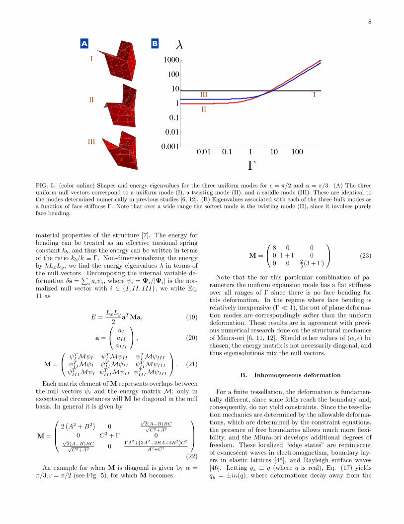
FIG. 5. (color online) Shapes and energy eigenvalues for the three uniform modes for ε = π/2 and α = π/3. (A) The threeuniform null vectors correspond to a uniform mode (I), a twisting mode (II), and a saddle mode (III). These are identical tothe modes determined numerically in previous studies [6, 12]. (B) Eigenvalues associated with each of the three bulk modes asa function of face stiffness Γ. Note that over a wide range the softest mode is the twisting mode (II), since it involves purelyface bending.

material properties of the structure [7]. The energy forbending can be treated as an effective torsional springconstant kb, and thus the energy can be written in termsof the ratio kb/k ≡ Γ. Non-dimensionalizing the energyby kLxLy, we find the energy eigenvalues λ in terms ofthe null vectors. Decomposing the internal variable de-formation δs =

∑i aiψi, where ψi = Ψi/|Ψi| is the nor-

malized null vector with i ∈ {I, II, III}, we write Eq.11 as

E =LxLy

2aTMa, (19)

a =

aIaIIaIII

, (20)

M =

ψTIMψI ψTIMψII ψTIMψIIIψTIIMψI ψTIIMψII ψTIIMψIIIψTIIIMψI ψTIIIMψII ψTIIIMψIII

. (21)

Each matrix element of M represents overlaps betweenthe null vectors ψi and the energy matrix M; only inexceptional circumstances will M be diagonal in the nullbasis. In general it is given by

M =

2(A2 +B2

)0

√2(A−B)BC√C2+A2

0 C2 + Γ 0√

2(A−B)BC√C2+A2

0ΓA2+(3A2−2BA+2B2)C2

A2+C2

(22)

An example for when M is diagonal is given by α =π/3, ε = π/2 (see Fig. 5), for which M becomes:

M =

8 0 00 1 + Γ 00 0 2

3 (3 + Γ)

(23)

Note that the for this particular combination of pa-rameters the uniform expansion mode has a flat stiffnessover all ranges of Γ since there is no face bending forthis deformation. In the regime where face bending isrelatively inexpensive (Γ� 1), the out of plane deforma-tion modes are correspondingly softer than the uniformdeformation. These results are in agreement with previ-ous numerical research done on the structural mechanicsof Miura-ori [6, 11, 12]. Should other values of (α, ε) bechosen, the energy matrix is not necessarily diagonal, andthus eigensolutions mix the null vectors.

B. Inhomogeneous deformation

For a finite tessellation, the deformation is fundamen-tally different, since some folds reach the boundary and,consequently, do not yield constraints. Since the tessella-tion mechanics are determined by the allowable deforma-tions, which are determined by the constraint equations,the presence of free boundaries allows much more flexi-bility, and the Miura-ori develops additional degrees offreedom. These localized “edge states” are reminiscentof evanescent waves in electromagnetism, boundary lay-ers in elastic lattices [45], and Rayleigh surface waves[46]. Letting qx ≡ q (where q is real), Eq. (17) yieldsqy = ±iκ(q), where deformations decay away from the

9

A B C D

E F

In[8]:= PlotB:1

k@p ê 3, p ê 2, qD>, 8q, 0, p<, PlotRange Ø 880, 4<, 80, 3<<, PlotStyle Ø ThickF

Out[8]=

1 2 3 40.0

0.5

1.0

1.5

2.0

2.5

3.0

In[9]:= PlotB:1

k@p ê 3, p ê 2, qD>, 8q, 0, p<,

PlotRange Ø 880, 4<, 80, 3<<, PlotStyle Ø Thick, Axes Ø FalseF

Out[9]=

�FIG. 6. (color online) Experimental observations of deformation localization in an 8 × 8 Miura-ori tessellation. (A) Anundeformed Miura-ori shows a regular periodic pattern. Under (B) small deformations, (C) large deformations, and (D) in thepresence of a “pop-through defect” (PTD) [7], the lattice distorts to accommodate the induced strain. (E) Qualitatively, theamount of deformation localization can be easily seen by a simple image subtraction between the deformed and undeformedstate. (F) Measuring strain along the horizontal axis as a function of unit cell position n relative to the location of thedisturbance shows a rapid decay for all three scenarios (points). For small and large amplitudes, the decays can be readilyfit to an exponential function with decay length ` (red/upper and black/lower lines), whereas for a PTD, the decay lengthcan be estimated to within 100%. Because the PTD induces an extensional distortion rather than a compression, the strain isoppositely signed. (Inset) Plotting the decay length against an approximate measure of the distortion wave vector q shows thelarger wave vector decays much more rapidly than the shorter wave vectors. Within errorbars, this measurement is consistentwith an inverse relationship between decay length and wave vector. The solid line is the theoretical prediction from Eq. 24 forε = π/2 and α = π/3.

boundaries of constant y with a length scale ` ≡ 1/κ(q),with

`(q) =1

2| sinh−1[ cosα sin(q/2)sin2 ε/2

]|. (24)

This localization length is readily observed in defor-mation experiments on Miura-ori sheets (see Fig. 6).Using laser-cut sheets of paper, an 8 × 8 Miura-ori isconstructed by folding the whole sheet using a planarangle of α = π/3 into the ground state given by ε = π/2(Fig. 6A). Inhomogeneous deformations are created us-ing both an external indenter to apply a displacement(Fig. 6B,C) and by placing reversible “pop-through de-fects” (Fig. 6D) [7]. The strain γn at each unit celln is measured such that γn = ∆wn/w, where ∆ww isthe change in width of the nth cell and w is the averagewidth for an undisturbed cell. As shown in Fig.6, thestrain decays exponentially away from the indenter witha decay length that is consistent (within error) with ourtheoretical predictions.

To examine these deformation modes more quantita-tively, we return to the “dispersion relation” given byEq. 17. There are two possible solutions to Eq. 17,corresponding to different decay directions, and thus the

null space of R corresponding to each of these branchesis two dimensional. We decompose δs(x) into a sum ofupward (in y) decaying and downward decaying modes,

δs = eiqx( [u1χ1e

−k(q)y + u2χ2e−k(q)y

]+ (25)[

d1η1ek(q)y + d2η2e

k(q)y] )

+ c.c.

The vectors χ1,2 correspond to the upward decayingmodes, while η1,2 the downward decaying modes. Notethat, since the values of the angles must be real, η1,2(q) =χ1,2(−q). In the long-wavelength limit, i.e. q � 1, wehave:

10

χ1 =

−CAq+CB(q−2i)AB02q

−CAq+CB(q+2i)AB00

CAq−CB(q−2i)AB00

CAq+CB(q+2i)AB02q

, χ2 =

− 2CA

00− 2C

A−2iq

0− 2C

A−2iq

0− 2C

A00

(26)

The nullspace, and thus the number of elementary ex-citations, for a finite-sized Miura-ori is actually differentthan for the limit q → 0. While this may seem counter-intuitive, the nature of the null vectors is inherently chi-ral, as indicated by the decomposition into upward anddownward decaying solutions. At q = 0, the dimension-ality of the nullspace is smaller because there is no dis-tinction between handedness for uniform deformation.

C. Miura-ori’s “soft modes”

The vectors χ1,2 govern the kinematic deformations ofMiura-ori, giving the possible solutions to the constraintequations. For a tessellation with an associated torsionalspring energy at each crease, the energy density per modemay be written in Fourier space as

E =LxLy

2c†(q)H(q)c(q), (27)

where

c(q) =

u1(q)u2(q)d1(q)d2(q)

, (28)

and H is the 2× 2 Hermitian block matrix ,

H =

(H0 H1

H†1 H†0

). (29)

The two independent blocks of H are given by

H0 =

(χ†1Mχ1 χ†1Mχ2

χ†2Mχ1 χ†2Mχ2

). (30)

and

H1 =

(χ†1Mη1 χ†1Mη2

χ†2Mη1 χ†2Mη2

). (31)

For finite wavenumber there are four modes of defor-mation. Typical eigenvalues of H(q) are shown in Fig.

7. The largest two eigenvalues are typically associatedwith changing ε, since there is an energetic cost even forvery small Γ. The typically smallest two eigenvalues cor-respond to twisting mode and a fourth mode that has noanalogue in the zero wavenumber case. This mode hasa qualitative shape that is similar to the twisting mode,and an energy that vanishes as q → 0, much like anacoustic mode in a crystal. Previous analyses of inhomo-geneous deformations have not found this mode, whichwe identify here as arising from the breaking of contin-uous symmetry when a boundary is added to one sideof the tessellation. The acoustic mode corresponds toan antisymmetric combination of upward and downwarddecaying modes; consequently, as q becomes smaller, thechange in fold angles associated with the combinationcancel, and only three modes appear at q = 0.

The modes that are softest depend not only on thestiffness of face bending, but on the ground state definedby ε0 (see Fig. 7). This stiffness dependence is in ac-cord with the previously predicted anisotropic in-planestiffness response [6, 13]. Additionally, since our analysisallows for arbitrary size and wavenumber, we are able tocapture the response of the previously unidentified acous-tic mode.

IV. DISCUSSION

While there has been numerical analysis of tessellationsin the past, our theoretical formulation provides severalkey insights into the design and understanding of origamimechanics. We not only analytically calculate expres-sions for first-order inhomogeneous deformations, but wefind an additional acoustic mode of deformation that hasnot been identified using numerics. Moreover, we havefound an analytical expression for a decay length thatarises in Miura-ori, and identify that these “soft modes”are edge states that cannot occur in an infinite tessel-lation. Indeed, the appearance of a single decay lengthand the ability to fully quantify the deformation modesusing a single wavenumber indicates that the boundariesof Miura-ori fully define the deformation state. We candirectly conclude from this that, unlike normal solids, thethe number of degrees of freedom scale with the perime-ter of a finite tessellation, rather than the area. Thisresult suggests that there are surface boundary statesthat can be used to probe the full deformation of thematerial, and hints at the connection between our workat recent studies on topological mechanics [38]. In fact,our mathematical formalism shares many parallels withthe topological mechanics of linkages [47–49], as well asthe more conventional literature concerning topologicalinsulators and semimetals [50–52]. It remains to be seenexactly how the symmetry and topology of the creasepattern affect the nature of chiral modes in origami, butthere is evidence to suggest that even slight modificationsof the crease pattern symmetry may lead to preferentiallydirected chiral states.

11

In[1980]:=

FoldedFormGraphics3D@twisttessD ê. OrigamiStyle@D

Out[1980]=

ListPlot@GetValue@twisttess, FoldAnglesDD

50 100 150 200 250 300

-2

-1

1

2

ArtTessellationSimulation.nb 19

q

�

�

�

In[1981]:= FoldedFormGraphics3D@saddletessD ê. OrigamiStyle@D

Out[1981]=

ListPlot@GetValue@tobjff, FoldAnglesDDListPlot@GetValue@saddletess, FoldAnglesDD

50 100 150 200 250 300

-2

-1

1

2

50 100 150 200 250 300

-2

-1

1

2

ArtTessellationSimulation.nb 17

I

In[1982]:= groundstatetess = FoldedFormGraphics3D@tobjffD ê. OrigamiStyle@D

Out[1982]=

faspecs = MakeStdFoldAngleSpecs@tobjD;faspecs = faspecs ê. 881, 90 °< Ø 81, 180 ê 7 °<, 81, -90 °< Ø 810, -180 ê 7 °<<;foldangles = MakeGraphFoldAngles@tobj, faspecsD;tobjff = FoldGraph3D@tobj, foldanglesD;groundstatetess2 = FoldedFormGraphics3D@tobjffD ê. OrigamiStyle@D

GetAllProperties@tobjffDGetAllProperties@tobjffD

In[1896]:= faspecs = MakeStdFoldAngleSpecs@tobjD;faspecs = faspecs ê. 881, 0< Ø 810, p ê 12<<;foldangles = MakeGraphFoldAngles@tobjff, faspecsD;saddletess = FoldGraph3D@tobjff, foldanglesD;

16 ArtTessellationSimulation.nb

II

III, IV

q

In[41]:= Block@8a = p ê 3, e = p ê 2<, Plot@NEn@MyA@a, eD, MyB@a, eD, MyCC@a, eD, q, 1, .10, 1, 10D,8q, 0, p<, PlotRange Ø All, BaseStyle Ø 8FontSize Ø 18<, PlotStyle Ø 8Thick, Black<DD

Block@8a = p ê 3, e = p ê 2<, Plot@NEn@MyA@a, eD, MyB@a, eD, MyCC@a, eD, q, 1, 1.0, 1, 10D,8q, 0, p<, PlotRange Ø All, BaseStyle Ø 8FontSize Ø 18<, PlotStyle Ø 8Thick, Black<DD

Block@8a = p ê 3, e = p ê 2<, Plot@NEn@MyA@a, eD, MyB@a, eD, MyCC@a, eD, q, 1, 10, 1, 10D,8q, 0, p<, PlotRange Ø All, BaseStyle Ø 8FontSize Ø 18<, PlotStyle Ø 8Thick, Black<DD

Out[41]=

0.5 1.0 1.5 2.0 2.5 3.0

5

10

15

Out[42]=

0.5 1.0 1.5 2.0 2.5 3.0

5

10

15

Out[43]=

0.5 1.0 1.5 2.0 2.5 3.0

5

10

15

2DMiuraArt_fiddle.nb 33

Out[1984]=

MiuraPlotNew.nb 9

Out[1985]=

10 MiuraPlotNew.nb

� = 0.1

� = 1

� = 10

� = 0.1

� = 1

� = 10

I

II

III,IV

BA Block@8a = p ê 2 - p ê 20, e = p ê 2<,Plot@NEn@MyA@a, eD, MyB@a, eD, MyCC@a, eD, q, 1, .10, 1, 10D, 8q, 0, p<,PlotRange Ø All, BaseStyle Ø 8FontSize Ø 18<, PlotStyle Ø 8Thick, Black<DD

Block@8a = p ê 2 - p ê 20, e = p ê 2<,Plot@NEn@MyA@a, eD, MyB@a, eD, MyCC@a, eD, q, 1, 1.0, 1, 10D, 8q, 0, p<,PlotRange Ø All, BaseStyle Ø 8FontSize Ø 18<, PlotStyle Ø 8Thick, Black<DD

Block@8a = p ê 2 - p ê 20, e = p ê 2<,Plot@NEn@MyA@a, eD, MyB@a, eD, MyCC@a, eD, q, 1, 10, 1, 10D, 8q, 0, p<,PlotRange Ø All, BaseStyle Ø 8FontSize Ø 18<, PlotStyle Ø 8Thick, Black<DD

0.5 1.0 1.5 2.0 2.5 3.0

1

2

3

4

0.5 1.0 1.5 2.0 2.5 3.0

1

2

3

4

0.5 1.0 1.5 2.0 2.5 3.0

1

2

3

4

5

2DMiuraArt_fiddle.nb 33

FIG. 7. (color online) Eigenvalues and mode shapes as a function of wavenumber for a given Γ. (A) Left: Mode structure fori) Γ = 0.1, ii) Γ = 1, and iii)Γ = 10, with ε = π/2 and α = π/3. At long wavelengths the saddle mode I is the stiffest for awide range of q, since it involves both bending of the faces and deformation of the angles away from the reference state. Right:Mode structure for i) Γ = 0.1, ii) Γ = 1, and iii) Γ = 10, with ε = π/2 and α = 9π/20. (B) Visualization of the basic modesfor q = π/6.

A great deal of this analysis can be carried through toother origami fold patterns. What is less clear, however,is how the number of degrees of freedom – the null spaceof R(q) – changes for different fold patterns. At theoutset it may seem coincidental that the matrix R(q) issquare. In fact, this behavior is likely more generic. Inparticular, the Miura-ori – with additional folds acrossthe faces – is composed of triangular sub-units. In anytriangulated origami fold pattern, vertices will tend tohave, on average, six folds. Hence, for V vertices (withV very large), we have 3V unique folds, and 3V degreesof freedom per vertex. Consequently, R(q) will be a 3V ×3V square matrix for sufficiently large V .

Finally, a great advantage to this approach is the abil-ity to separate the topological nature of the crease pat-

tern from the geometry of the vertex. The ability to iso-late mechanical deformations or elementary excitationsin exotic materials is of great interest in quantum con-densed matter [38], amorphous solids [53–55], and com-plex fluids [56]. Our theoretical framework for origamitessellations bridges the gap between the origami me-chanics literature and a theory of origami meta-materialsby identifying the constraint-based nature of the foldingmechanisms and applying well-known methods of analy-sis from solid state physics and lattice mechanics.

The authors acknowledge interesting and helpful dis-cussions with Tom Hull, Robert Lang, Tomohiro Tachi,Scott Waitukaitis, Martin van Hecke, and Michael Assis.We also thank F. Parish for help with the laser cutter.This work was funded by the National Science Founda-tion through award EFRI ODISSEI-1240441.

[1] T. Tachi, in Symposium of the International Associationfor Shell and Spatial Structures (50th. 2009. Valencia).Evolution and Trends in Design, Analysis and Construc-tion of Shell and Spatial Structures: Proceedings (Edito-rial de la Universitat Politecnica de Valencia., 2009).

[2] T. Tachi, in Proceedings of the International Associa-tion for Shell and Spatial Structures (IASS) Symposium,Vol. 12 (2010) pp. 458–460.

[3] T. Tachi, in Symposium of the International Associationfor Shell and Spatial Structures (50th. 2009. Valencia).Evolution and Trends in Design, Analysis and Construc-

tion of Shell and Spatial Structures: Proceedings (Edito-rial de la Universitat Politecnica de Valencia., 2010).

[4] E. Hawkes, B. An, N. Benbernou, H. Tanaka, S. Kim,E. Demaine, D. Rus, and R. Wood, Proc. Natl. Acad.Sci. U.S.A. 107, 12441 (2010).

[5] M. A. Dias, L. H. Dudte, L. Mahadevan, and C. D.Santangelo, Phys. Rev. Lett. 109, 114301 (2012).

[6] M. Schenk and S. D. Guest, Proc. Natl. Acad. Sci. U.S.A.110, 3276 (2013).

[7] J. L. Silverberg, A. A. Evans, L. McLeod, R. C. Hayward,T. Hull, C. D. Santangelo, and I. Cohen, Science 345,

12

647 (2014).[8] J.-H. Na, A. A. Evans, J. Bae, M. C. Chiappelli, C. D.

Santangelo, R. J. Lang, T. C. Hull, and R. C. Hayward,Adv. Mater. (2014).

[9] C. Py, P. Reverdy, L. Doppler, J. Bico, B. Roman, andC. N. Baroud, Phys. Rev. Lett. 98, 156103 (2007).

[10] J. Solomon, E. Vouga, M. Wardetzky, and E. Grinspun,in Computer Graphics Forum, Vol. 31 (Wiley Online Li-brary, 2012) pp. 1567–1576.

[11] M. Schenk and S. Guest, Folded shell structures, Ph.D.thesis, PhD thesis (Univ of Cambridge, Cambridge,United Kingdom) (2011).

[12] M. Schenk and S. D. Guest, Origami 5, 291 (2011).[13] Z. Wei, Z. Guo, L. Dudte, H. Liang, and L. Mahadevan,

Phys. Rev. Lett. 110, 215501 (2013).[14] K. Abdul-Sater, F. Irlinger, and T. C. Lueth, J. Mech.

Robot. 5, 031005 (2013).[15] S. Waitukaitis, R. Menaut, B. G.-g. Chen, and M. van

Hecke, Phys. Rev. Lett. 114, 055503 (2015).[16] B. H. Hanna, J. M. Lund, R. J. Lang, S. P. Magleby, and

L. L. Howell, Smart Mater. Struct. 23, 094009 (2014).[17] N. P. Bende, A. A. Evans, S. Innes-Gold, L. A. Marin,

I. Cohen, R. C. Hayward, and C. D. Santangelo, arXivpreprint arXiv:1410.7038 (2014).

[18] J. B. Pendry, D. Schurig, and D. R. Smith, Science 312,1780 (2006).

[19] M. Kadic, T. Buckmann, N. Stenger, M. Thiel, andM. Wegener, Appl. Phys. Lett. 100, 191901 (2012).

[20] S. Brule, E. Javelaud, S. Enoch, and S. Guenneau, Phys.Rev. Lett. 112, 133901 (2014).

[21] M. Farhat, S. Guenneau, and S. Enoch, Phys. Rev. Lett.103, 024301 (2009).

[22] N. Stenger, M. Wilhelm, and M. Wegener, Phys. Rev.Lett. 108, 014301 (2012).

[23] J. Shim, S. Shan, A. Kosmrlj, S. H. Kang, E. R. Chen,J. C. Weaver, and K. Bertoldi, Soft Matter 9, 8198(2013).

[24] A. A. Evans and A. J. Levine, Phys. Rev. Lett. 111,038101 (2013).

[25] Y. Zhang, E. A. Matsumoto, A. Peter, P.-C. Lin, R. D.Kamien, and S. Yang, Nano Lett. 8, 1192 (2008).

[26] E. A. Matsumoto and R. D. Kamien, Phys. Rev. E 80,021604 (2009).

[27] K. Bertoldi, P. M. Reis, S. Willshaw, and T. Mullin,Adv. Mater. 22, 361 (2010).

[28] E. A. Matsumoto and R. D. Kamien, Soft Matter 8,11038 (2012).

[29] J. T. B. Overvelde, S. Shan, and K. Bertoldi, Adv.Mater. 24, 2337 (2012).

[30] “Tessellatica,” http://www.langorigami.com/science/

computational/tessellatica/tessellatica.php.[31] C. Yoon, R. Xiao, J. Park, J. Cha, T. D. Nguyen, and

D. H. Gracias, Smart Mater. Struct. 23, 094008 (2014).[32] Y. Liu, J. K. Boyles, J. Genzer, and M. D. Dickey, Soft

Matter 8, 1764 (2012).[33] L. Ionov, Soft Matter 7, 6786 (2011).[34] G. Stoychev, N. Puretskiy, and L. Ionov, Soft Matter 7,

3277 (2011).[35] D. A. Huffman, IEEE Trans. Computers 25, 1010 (1976).[36] T. C. Hull and s.-m. belcastro, Linear Algebra Appl. 348,

273 (2002).[37] R. Hutchinson and N. Fleck, J. Mech. Phys. Solids 54,

756 (2006).[38] C. Kane and T. Lubensky, Nature Phys. 10, 39 (2014).[39] F. Lechenault, B. Thiria, and M. Adda-Bedia, Phys.

Rev. Lett. 112, 244301 (2014).[40] J. L. Silverberg, J.-H. Na, A. A. Evans, B. Liu, T. C.

Hull, C. D. Santangelo, R. J. Lang, R. C. Hayward, andI. Cohen, Nature materials 14, 389 (2015).

[41] L. Mahadevan and S. Rica, Science 307, 1740 (2005).[42] A. E. Shyer, T. Tallinen, N. L. Nerurkar, Z. Wei, E. S. Gil,

D. L. Kaplan, C. J. Tabin, and L. Mahadevan, Science342, 212 (2013).

[43] E. D. Demaine, M. L. Demaine, V. Hart, G. N. Price,and T. Tachi, Graphs and Combinatorics 27, 377 (2011).

[44] T. Witten, Rev. Mod. Phys. 79, 643 (2007).[45] A. S. Phani and N. A. Fleck, J. Appl. Mech. 75, 021020

(2008).[46] J. W. Strutt and L. Rayleigh, Proceedings of the London

Mathematical Society 17, 4 (1885).[47] B. G.-g. Chen, N. Upadhyaya, and V. Vitelli, Proceed-

ings of the National Academy of Sciences 111, 13004(2014).

[48] J. Paulose, B. G.-g. Chen, and V. Vitelli, Nature Phys.(2015).

[49] J. Paulose, A. S. Meeussen, and V. Vitelli, arXiv preprintarXiv:1502.03396 (2015).

[50] M. Z. Hasan and C. L. Kane, Rev. Mod. Phys. 82, 3045(2010).

[51] X.-L. Qi and S.-C. Zhang, Rev. Mod. Phys. 83, 1057(2011).

[52] H. C. Po, Y. Bahri, and A. Vishwanath, arXiv preprintarXiv:1410.1320 (2014).

[53] K. Sun, A. Souslov, X. Mao, and T. Lubensky, Proc.Natl. Acad. Sci. U.S.A. 109, 12369 (2012).

[54] X. Mao, N. Xu, and T. Lubensky, Phys. Rev. Lett. 104,085504 (2010).

[55] M. Wyart, S. Nagel, and T. Witten, Europhys. Lett. 72,486 (2005).

[56] E. Lerner, G. During, and M. Wyart, Proc. Natl. Acad.Sci. U.S.A. 109, 4798 (2012).