Lattice Flavour Physics

N. Tantalo

Rome University “Tor Vergata” and INFN sez. “Tor Vergata”

22-07-2011

lattice QCD errors

in order to improve errors on hadronic matrix elements by using lattice techniques one has to pay (the currency isTFlops × year)

L.Del Debbio, L.Giusti, M.Luscher, R.Petronzio, N.T. JHEP 0702 (2007) 056

TFlops × year = 0.03(Nconf

100

) ( 20 MeV

mud

) ( Lt

2Ls

) ( Ls

3 fm

)5 ( 0.1 fm

a

)6

∼ 0.03(Nconf

100

) ( 20 MeV

mud

) ( Nt × Ns

64× 32

)∼3

i.e., as a rule of thumb, we can say that fixed the pion mass and given a supercomputer we have a budgetquantified in terms of number of points of our lattice. . .

then we have to decide if to spend this budget for light quark physics (big volumes) or for heavy quark physics(small lattice spacings)

important:

using this formula today is a conservative estimate: several other algorithmic improvements since 2007(Luscher deflation acceleration, etc.)

on the other hand sampling errors do enter our game and we are neglecting them to obtain our estimates

for a detailed discussion of these problems and for a proposal to solve them see (and references therein)M. Luscher, S. Schaefer arXiv:1105.4749

lattice QCD errors

let’s play the ”lattice effective theory” game invented by: S.Sharpe @ Orsay 2004 ”LQCD, present and future”V. Lubicz @ XI SuperB Workshop LNF 2009

concerning continuum extrapolations, we imagine to simulate an O(a) improved theory at amin and√

2amin andto extrapolate linearly in a2

Ophys= Olatt

{1 + c2(aΛQCD)

2+ c3(aΛQCD)

3+ . . .

}→

∆O

O= (23/2 − 1) c3 (alightΛQCD)

3

Ophys= Olatt

{1 + c2(amh)

2+ c3(amh)

3+ . . .

}→

∆O

O= (23/2 − 1) c3 (aheavymh)

3

we assume c3 ∼ 1 (if c3 = 0 usually c4 large) and set the goal precision to 1%, getting

scale (GeV ) a (fm) Nt × Ns @ 3fm Pflops × y Nt × Ns @ 4fm Pflops × y

0.5 0.069 96 × 48 10−3 128 × 64 2 × 10−3

2.0 0.017 360 × 180 1 480 × 240 5

4.0 0.009 720 × 360 60 960 × 480 340

today, large lattice collaborations have access to the computer power required to accommodate low energyscales, so. . .

(pseudoscalar) light meson’s physics at 1% level today

BMW, arXiv:1011.2711

100 200 300 400M![MeV]

1

2

3

4

5

6

L[fm]

"=3.8"=3.7"=3.61"=3.5"=3.31

0.1%

0.3%1%

Figure 1: Summary of our simulation points. The pion masses and the spatial sizes of thelattices are shown for our five lattice spacings. The percentage labels indicate regions, in whichthe expected finite volume effect [3] onMπ is larger than 1%, 0.3% and 0.1%, respectively. Inour runs this effect is smaller than about 0.5%, but we still correct for this tiny effect.

In our view, item 2 marks the beginning of a new era in numerical lattice QCD, because itavoids an extrapolation in quark masses which, generically, requires strong assumptions, thusrelinquishing the first-principles approach (see the discussion in [1]).

To give the reader an overview of where we are in terms of simulated pion massesMπ andspatial box sizes L, a graphical survey of (some of) our simulation points is provided in Fig. 1(with more details given in Sec. 5). We have data at 5 lattice spacings in the range 0.054−0.116 fm, with pion masses down to ∼120 MeV and box sizes up to ∼6 fm. Comparison withChiral Perturbation suggests that our finite volume effects are typically below 0.5%, and closeto the physical mass point (which is the most relevant part) even smaller. Still, we correct forthem by means of Chiral Perturbation Theory [3], and test the correctness of this predictionthrough explicit finite volume scaling runs (see below).

The remainder of this paper is organized as follows. In Sec. 2 details are given concerningthe action and algorithm employed, while Sec. 3 specifies how one determines the HMC forcewith HEX smeared clover fermions. Our choice of the scale setting procedure and of the in-put masses is discussed in Sec. 4, with simulation parameters tabulated in Sec. 5. Checks ofalgorithmic stability are summarized in Sec. 6, while autocorrelation and (practical) ergodicityissues are reported in Sec. 7. To corroborate the good scaling properties of our action, explicittests of the scaling of hadron masses in Nf =3 QCD are carried out, see Sec. 8. Details of how

4

from the previous slide we learn that (standard) light meson’s observable should be under control now!

chiral extrapolations are no more a source of concern in 2011 (not only BMW collaboration,. . . )

. . . at least if one is spending his own budget for simulating big volumes

FK/Fπ & FKπ+ (0) summary from FLAG

G.Colangelo et al. arXiv:1011.4408

arXiv:1005.2323 [hep-ph]

arXiv:1011.4408 [hep-lat]

F L A G

THE

OR

Y: L

ATTI

CE

QC

DE

XP

ER

IME

NTS

giovedì 14 aprile 2011

FKπ+ (0) = 0.956(3)(4) ∼ 0.5%

FK

Fπ= 1.193(5) ∼ 0.5%

are these error estimates reliable? i.e. can we trust our predictions?

within the lattice community we could discuss all the life about that, but. . .

FK/Fπ & FKπ+ (q2) can be measured (within SM)

we do have a lot of precise experimental measurements in the quark flavour sector of the standard model that,combined with CKM unitarity (first row), allow us to measure hadronic matrix elements

a simple example from FLAVIAnet kaon working group M.Antonelli et al. Eur.Phys.J.C69

∣∣∣∣ VusFKVud Fπ

∣∣∣∣ = 0.27599(59)

∣∣∣VusFKπ+ (0)

∣∣∣ = 0.21661(47)

|Vud |2 + |Vus|2 = 1

|Vud | = 0.97425(22)

where |Vud | comes by combining 20 super-allowed nuclear β-decays and |Vub| has been neglected because smallerthan the uncertainty on the other terms, combine to give

|Vus| = 0.22544(95)

FKπ+ (0) = 0.9608(46) FKπ

+ (0)∣∣∣lattice

= 0.956(3)(4)

FK

Fπ= 1.1927(59)

FK

Fπ

∣∣∣∣lattice

= 1.193(5)

20 M. Antonelli et al.: Evaluation of |Vus| and Standard Model tests from kaon data

Mode |Vus|f+(0) % err BR τ ∆ Int Correlation matrix (%)KL → πeν 0.2163(6) 0.26 0.09 0.20 0.11 0.06 +55 +10 +3 0KL → πµν 0.2166(6) 0.29 0.15 0.18 0.11 0.08 +6 0 +4KS → πeν 0.2155(13) 0.61 0.60 0.03 0.11 0.06 +1 0K± → πeν 0.2160(11) 0.52 0.31 0.09 0.40 0.06 +73K± → πµν 0.2158(14) 0.63 0.47 0.08 0.39 0.08Average 0.2163(5)

Table 14. Values of |Vus|f+(0) as determined from each kaon decay mode, with approximate contributions to relative uncertainty(% err) from branching ratios (BR), lifetimes (τ ), combined effect of δK!

EM and δK!SU(2) (∆), and phase space integrals (Int).

comparison with Eq. (9), rµe is equal to the ratio g2µ/g2

e ,with g! the coupling strength at the W → !ν vertex. Inthe SM, rµe = 1.

Before the advent of the new BR measurements de-scribed in Sects. 3.2 and 3.4, the values of |Vus|f+(0) fromKe3 and Kµ3 rates were in substantial disagreement. Us-ing the KL and K± BRs from the 2004 edition of the PDGcompilation [100] (and assuming current values for the I!3

and δK!EM), we obtain rµe = 1.013(12) for K± decays and

1.040(13) for KL decays.As noted in Sect. 3.2, the new BR measurements pro-

cure much better agreement. From the entries in Table 14,we calculate rµe separately for charged and neutral modes(including the value of |Vus|f+(0) from KS → πeν de-cays, though this has little impact) and obtain 0.998(9)and 1.003(5), respectively. The results are compatible; theaverage value is rµe = 1.002(5). As a statement on thelepton-flavor universality hypothesis, we note that the sen-sitivity of this test approaches that obtained with π →!ν decays ((rµe) = 1.0042(33) [138]) and τ → !νν de-cays ((rµe) = 1.000(4) [139]). Alternatively, if the lepton-universality hypothesis is assumed to be true, the equiva-lence of the values of |Vus|f+(0) from Ke3 and Kµ3 demon-strates that the calculation of the long-distance correc-tions δK!

EM is accurate to the per-mil level.

4.4 Determination of |Vus/Vud| × fK/fπ

As noted in Sect. 2.1, Eq. (2) allows the ratio |Vus/Vud| ×fK/fπ to be determined from experimental information onthe radiation-inclusive K!2 and π!2 decay rates. The lim-iting uncertainty is that from BR(Kµ2(γ)), which is 0.28%as per Table 6. Using this, together with the value of τK±

from the same fit and Γ (π± → µ±ν) = 38.408(7) µs−1 [87]we obtain

|Vus/Vud| × fK/fπ = 0.2758(5). (55)

4.5 Test of CKM unitarity

We determine |Vus| and |Vud| from a fit to the resultsobtained above. As starting points, we use the value|Vus|f+(0) = 0.2163(5) given in Table 14, together withthe lattice QCD estimate f+(0) = 0.959(5) (Eq. (17)).We also use the result |Vus/Vud| × fK/fπ = 0.2758(5)

0.224

0.226

0.228

0.972 0.974 0.976

Vud

V us

0.224

0.226

0.228

0.972 0.974 0.976

Vud (0+ ! 0+)

Vus/Vud (Kµ2)

Vus (Kl3)

fit withunitarity

fit

unitarity

Fig. 10. Results of fits to |Vud|, |Vus|, and |Vus/Vud|.

discussed in Sect. 4.4 together with the lattice estimatefK/fπ = 1.193(6) (Sect. 2.1.1). Thus we have

|Vus| = 0.2254(13) [K!3 only],

|Vus/Vud| = 0.2312(13) [K!2 only].(56)

Finally, we use the evaluation |Vud| = 0.97425(22) froma recent survey [140] of half-life, decay-energy, and BRmeasurements related to 20 superallowed 0+ → 0+ nu-clear beta decays, which includes a number of new, high-precision Penning-trap measurements of decay energies,as well as the use of recently improved electroweak ra-diative corrections [141] and new isospin-breaking correc-tions [142], in addition to other improvements over pastsurveys by the same authors. Our fit to these inputs gives

|Vud| = 0.97425(22),

|Vus| = 0.2253(9) [K!3, K!2, 0+ → 0+],

(57)

with χ2/ndf = 0.014/1 (P = 91%) and negligible corre-lation between |Vud| and |Vus|. With the current world-average value, |Vub| = 0.00393(36) [87], the first-row uni-tarity sum is then ∆CKM = |Vud|2 + |Vus|2 + |Vub|2 − 1 =−0.0001(6); the result is in striking agreement with theunitarity hypothesis. (Note that the contribution to thesum from |Vub| is essentially negligible.) As an alternateexpression of this agreement, we may state a value for

FK/Fπ & FKπ+ (q2) reducing the error

there are two sources of isospin breaking effects,

mu 6= md︸ ︷︷ ︸QCD

qu 6= qd︸ ︷︷ ︸QED

in the particular and (lucky) case of these observables, the correction to the isospin symmetric limit due to thedifference of the up and down quark masses (QCD) can be estimated in chiral perturbation theory,

FKπ+ (0) = 0.956(3)(4) ∼ 0.5%

FK+π0+ (q2)

FK0π−+

(q2)− 1

QCD

= 0.029(4)

A. Kastner, H. Neufeld Eur.Phys.J.C57 (2008)

FKFπ

= 1.193(5) ∼ 0.5%

(F

K+/Fπ+

FK/Fπ− 1

)QCD

= −0.0022(6)

V. Cirigliano, H. Neufeld arXiv:1102.0563

reducing the error on these quantities without taking into account isospin breaking is useless. . .

QCD isospin breaking on the lattice

RM123 collaboration, PRELIMINARY!

〈O〉 + ∆〈O〉 =

∫DU e−Sg [U ]−Sf [U ] O∫

DU e−Sg [U ]−Sf [U ]=

∫DU e

−Sg [U ]−S0f [U ]

(1 + ∆mS3)O∫DU e

−Sg [U ]−S0f [U ]

(1 + ∆mS3)

= 〈O〉 + ∆m〈S3 O〉

0 0.01 0.02 0.03 0.04 0.05 0.06ml

MS,2GeV (GeV)

-2.7

-2.6

-2.5

-2.4

-2.3

-2.2

-2.1

-2

-1.9

-1.8

∆M2 K

a = 0.098 fma = 0.085 fma = 0.067 fma = 0.054 fmPhysical point

Chiral extrapolation of ∆M2K

taking as input

∆MK = MK0 − MK+ −∆MQEDK = −6.0(6) MeV

we get

(md − mu)MS,2GeV

= 2.28(6)(24) MeV

0 0.01 0.02 0.03 0.04 0.05 0.06ml

MS,2GeV (GeV)

-0.6

-0.5

-0.4

-0.3

-0.2

-0.1

0

∆fK

/δm

a = 0.098 fma = 0.085 fma = 0.067 fma = 0.054 fmPhysical point

Chiral extrapolation of ∆fK/δm

(FK+/F

π+

FK/Fπ− 1

)QCD

= −0.0034(3)(3)

to be compared with the χ-pt estimate−0.0022(6)

BK summary from FLAG

G.Colangelo et al. arXiv:1011.4408

Collaboration Ref. Nf publ

icat

ion

stat

us

cont

inuu

mex

trap

olat

ion

chiral

extr

apolat

ion

finitevo

lum

ere

norm

alizat

ion

runn

ing

BK BK

Kim 09 [252] 2+1 C ! • • " • 0.512(14)(34) 0.701(19)(47)

Aubin 09 [240] 2+1 A • !! • ! • 0.527(6)(21) 0.724(8)(29)

RBC/UKQCD 09 [253] 2+1 C • • ! ! • 0.537(19) 0.737(26)

RBC/UKQCD 07A, 08 [84, 254] 2+1 A " • ! ! • 0.524(10)(28) 0.720(13)(37)

HPQCD/UKQCD 06 [255] 2+1 A " •∗ ! " • 0.618(18)(135) 0.83(18)

ETM 09D [256] 2 C ! • • ! • 0.52(2)(2) 0.73(3)(3)

JLQCD 08 [250] 2 A " • " ! • 0.537(4)(40) 0.758(6)(71)

RBC 04 [257] 2 A " " "† ! • 0.495(18) 0.699(25)

UKQCD 04 [258] 2 A " " "† " • 0.49(13) 0.69(18)

Table 15: Results for the kaon B-parameter together with a summary of systematic errors.The symbol •∗ means that this result has been obtained with only two “light” sea quarkmasses. The symbol "† means that these results have been obtained at (MπL)min > 4 in alattice box with a spatial extension L < 2 fm. The symbol !! means that, in this mixedaction computation, the lightest valence pion weighs ∼ 230 MeV, while the lightest sea taste-pseudoscalar, used in the chiral fits, weighs ∼ 370 MeV.

value of a, which is in good agreement with the published estimate in [84, 254]. This indicatesthat discretization effects for BK computed using domain wall fermions appear to be smallat the present level of accuracy. In ref. [260] RBC/UKQCD have also investigated the effectsof residual chiral symmetry breaking induced by the finite extent of the 5th dimension in thedomain wall fermion formulation and found that the mixing of Q∆S=2 with operators of oppo-site chirality was negligibly small. The renormalization factors used by HPQCD/UKQCD 06are based on perturbation theory at one loop, which is by far the biggest source of systematicuncertainty quoted by these authors. The same is true for the new, preliminary result byKim et al. [261].

In view of the above, we believe that the most technically advanced, published estimatefor BK to date (with Nf = 2 + 1) is that of Aubin 09, which combines data computed at twovalues of the lattice spacing. Besides the usual systematic uncertainties listed in Table 15,they quote a 0.8% systematic error due to the setting of the physical scale and the calibrationof the down and strange quark masses. Their biggest single systematic uncertainty of 3.2% isassociated with the error on the renormalization factor, which links the B-parameter of thebare operator to that in the MS-scheme. Therefore, for QCD with Nf = 2 + 1 flavours, wequote

Nf = 2 + 1 : BK = 0.527(6)(21) BK = 0.724(8)(29) . (82)

64

the average is obtained by considering nf = 2 + 1 results only (no debate!) and is

BK (2GeV) = 0.527(6)(21) BK = 0.724(8)(29) ∼ 4%

the error is bigger than 1% because the systematics due to the renormalization of the four fermion operator is∼ 3%

latest BK at 1%

BMW collaboration arXiv:1106.3230

0.46

0.48

0.5

0.52

0.54

0.56

0.58

0.6

0 0.02 0.04 0.06 0.08 0.1 0.12 0.14 0.16

B KR

I (3.5

GeV

)

M 2[GeV2]

a 0.093 fma 0.076 fma 0.066 fma 0.054 fm

cont-limit

FIG. 5. Combined continuum extrapolation and interpolation to physical quark mass for a typical

Taylor fit out of our 5760 fits. The filled square represents our result for BRIK (3.5 GeV), the dashed

vertical line the physical pion mass. The interpolation in the quark mass is both mild and fully

under control.

0.49

0.5

0.51

0.52

0.53

0.54

0.55

0.56

0 0.005 0.01 0.015 0.02 0.025 0.03 0.035

B KR

I (3.5

GeV

)

sa[fm]

FIG. 6. Continuum extrapolation of BRIK (a, 3.5 GeV) obtained from the fit in Fig. 5.

reads

BRIK (3.5 GeV) = 0.5348(57)stat(34)sys (7)

where the individual contributions to the systematic error originate from the mixing terms

(0.0026), extrapolation into the continuum (0.0018), different chiral fit forms (0.0011), vari-

ation in the plateau range (0.0007) and the extraction of the renormalization constant

(0.0002).

For the reader’s convenience, we convert our main result of (7) into the MS-NDR scheme

and into the RGI value BK . We do so by using the NLO anomalous dimensions of [10, 11] and

the beta function at the highest available loop order [19]. It is notoriously difficult to reliably

assess the truncation error of a perturbative series, particularly in the 68% probability sense

7

0.46

0.48

0.5

0.52

0.54

0.56

0.58

0.6

0 0.02 0.04 0.06 0.08 0.1 0.12 0.14 0.16

B KR

I (3.5

GeV

)

M 2[GeV2]

a 0.093 fma 0.076 fma 0.066 fma 0.054 fm

cont-limit

FIG. 5. Combined continuum extrapolation and interpolation to physical quark mass for a typical

Taylor fit out of our 5760 fits. The filled square represents our result for BRIK (3.5 GeV), the dashed

vertical line the physical pion mass. The interpolation in the quark mass is both mild and fully

under control.

0.49

0.5

0.51

0.52

0.53

0.54

0.55

0.56

0 0.005 0.01 0.015 0.02 0.025 0.03 0.035

B KR

I (3.5

GeV

)

sa[fm]

FIG. 6. Continuum extrapolation of BRIK (a, 3.5 GeV) obtained from the fit in Fig. 5.

reads

BRIK (3.5 GeV) = 0.5348(57)stat(34)sys (7)

where the individual contributions to the systematic error originate from the mixing terms

(0.0026), extrapolation into the continuum (0.0018), different chiral fit forms (0.0011), vari-

ation in the plateau range (0.0007) and the extraction of the renormalization constant

(0.0002).

For the reader’s convenience, we convert our main result of (7) into the MS-NDR scheme

and into the RGI value BK . We do so by using the NLO anomalous dimensions of [10, 11] and

the beta function at the highest available loop order [19]. It is notoriously difficult to reliably

assess the truncation error of a perturbative series, particularly in the 68% probability sense

7

BK (2GeV) = 0.569(6)(4)(6) BK = 0.779(8)(5)(8) ∼ 1.6%

although Wilson-like fermions (wrong chirality mixings) small systematics from renormalization constants. . . (??)

quite surprising!!. . . on the other hand, on large volumes (∼ 6 fm), small lattice spacings (∼ 0.05 fm) and physicalpion masses one expects continuum-like behavior

in better agreement with unitarity triangle analyses

can we do better?

−→ H∆S=1W H∆S=1

W −→H∆S=2

W

BK parametrizes the mixing of the neutral Kaons in the effective theory in which both the W bosons and the up-typequarks have been integrated out,

BK (µ) =

⟨K∣∣H∆S=2

W (µ) |K〉83 F2

K M2K

in order to be used in εK formula, the figures in the previous slides have to be corrected for a factor parametrizing longdistance contributions

A.Buras, D.Guadagnoli Phys.Rev. D78 (2008)J.Laiho, E.Lunghi, R.S. Van de Water Phys.Rev. D81 (2010)

BK = κε BlatticeK κε ' 0.92

in order to do better on this process, we should be able to make a step backward and compute on the lattice the longdistance contributions,

⟨K∣∣ T{∫

d4x H∆S=1W (x;µ) H∆S=1

W (0;µ)

}|K〉

to this end, we should be able to make sense of the previous quantity in euclidean space

G.Isidori, G.Martinelli, P.Turchetti Phys.Lett. B633 (2006)

N. Crist arXiv:1012.6034

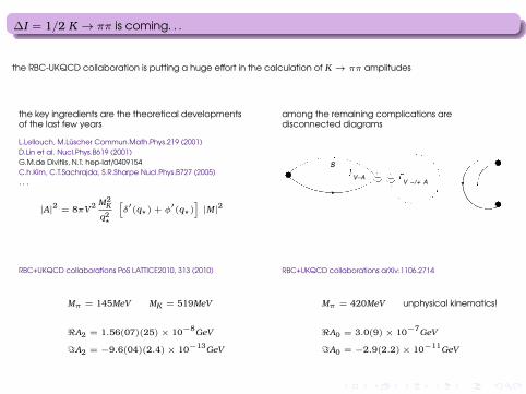
∆I = 1/2 K → ππ is coming. . .

the RBC-UKQCD collaboration is putting a huge effort in the calculation of K → ππ amplitudes

the key ingredients are the theoretical developmentsof the last few years

L.Lellouch, M.Luscher Commun.Math.Phys.219 (2001)D.Lin et al. Nucl.Phys.B619 (2001)G.M.de Divitiis, N.T. hep-lat/0409154C.h.Kim, C.T.Sachrajda, S.R.Sharpe Nucl.Phys.B727 (2005). . .

|A|2 = 8πV2 M2K

q2?

[δ′(q?) + φ

′(q?)

]|M|2

among the remaining complications aredisconnected diagrams

sV−A

V − /+ A

sV−A

V − /+ A

33©/35© 34©/36©

sV−A

V − /+ A

s sV−A

V − /+ A

s

37©/39© 38©/40©

sV−A

V − /+ A

sV−A

V − /+ A

41©/43© 42©/44©

s

V−A

V − /+ A

ss

V−A

V − /+ A

s

45©/47© 46©/48©

FIG. 6: Diagrams for the sixteen type4 K0 → ππ contractions.

A0,7(tπ, top, tK) = i

√3

2{− 3© − 7© + 11© + 15© + 19© (6g)

− 23© + 27© + 31© − 35© + 39© − 43© − 47©}

A0,8(tπ, top, tK) = i

√3

2{− 4© − 8© + 12© + 16© + 20© (6h)

− 24© + 28© + 32© − 36© + 40© − 44© − 48©}

A0,9(tπ, top, tK) = i

√3

2{− 1© − 5© + 9© + 13© + 17© (6i)

− 21© + 25© + 29© − 33© + 37© − 41© − 45©}

A0,10(tπ, top, tK) = i

√3

2{− 2© − 6© + 10© + 14© + 18© (6j)

− 22© + 26© + 30© − 34© + 38© − 42© − 46©},

where the factor i comes from our definition of the interpolation operator for the mesons,

12

RBC+UKQCD collaborations PoS LATTICE2010, 313 (2010)

Mπ = 145MeV MK = 519MeV

<A2 = 1.56(07)(25)× 10−8GeV

=A2 = −9.6(04)(2.4)× 10−13GeV

RBC+UKQCD collaborations arXiv:1106.2714

Mπ = 420MeV unphysical kinematics!

<A0 = 3.0(9)× 10−7GeV

=A0 = −2.9(2.2)× 10−11GeV

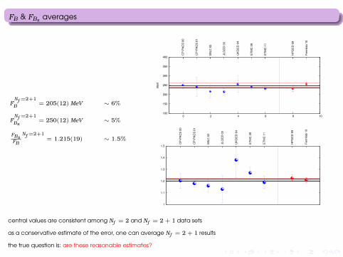
FB & FBs averages

FNf =2+1

B = 205(12) MeV ∼ 6%

FNf =2+1

Bs= 250(12) MeV ∼ 5%

FBsFB

Nf =2+1= 1.215(19) ∼ 1.5%

100

150

200

250

300

350

400

0 2 4 6 8 10

CP

-PA

CS

00

CP

-PA

CS

01

MIL

C 0

2

JLQ

CD

03

UK

QC

D 0

4

ET

MC

09

ET

MC

11

HP

QC

D 0

9

Ferm

ilab 1

0

MeV

1

1.1

1.2

1.3

1.4

1.5

CP

-PA

CS

00

CP

-PA

CS

01

MIL

C 0

2

JLQ

CD

03

UK

QC

D 0

4

ET

MC

09

ET

MC

11

HP

QC

D 0

9

Ferm

ilab 1

0

central values are consistent among Nf = 2 and Nf = 2 + 1 data sets

as a conservative estimate of the error, one can average Nf = 2 + 1 results

the true question is: are these reasonable estimates?

BB & BBs averages

0.6

0.7

0.8

0.9

1

1.1

1.2

UK

QC

D 0

0

AP

E 0

0

SP

QC

DR

01

JLQ

CD

02

JLQ

CD

03

HP

QC

D09

0.6

0.7

0.8

0.9

1

1.1

1.2

UK

QC

D 0

0

AP

E 0

0

SP

QC

DR

01

JLQ

CD

02

JLQ

CD

03

HP

QC

D09

a single Nf = 2 + 1 calculation, that combines with FBq to give

FBs

√BBs

Nf =2+1= 233(14) MeV ∼ 6% ξ

Nf =2+1

B = 1.237(32) ∼ 2.5%

again, are these reasonable estimates?

we usually spend all our budget for big volumes

by simulating b-quarks on the same volumes that we use to extract light meson’s physics we have to extrapolate in1/mh , (linear extrapolation from mh and

√2mh )

Ophys= Olatt

1 + b1ΛQCD

mh+ b2

(ΛQCD

mh

)2

+ . . .

→ ∆O

O=

b2

2

(ΛQCD

mh

)2

∼ 2÷ 3%

→∆OB

OB∝

√√√√a2n

(1

ΛQCDL

)2n

+ b22

(ΛQCD

mh

)4

+ c23(amh)6 ∼ 3÷ 4%

this can be considered a rough estimate of the bigger errors on B mesons’s observables

Nt × Ns Pflops × y scale (GeV ) a (fm) L (fm)

96× 48 10−3 0.5 0.069 3 fm96× 48 10−3 2.0 0.017 0.8 fm96× 48 10−3 4.0 0.009 0.4 fm

360× 180 1 0.5 0.069 12 fm360× 180 1 2.0 0.017 3 fm360× 180 1 4.0 0.009 1.5 fm

in case of b-physics it (may be) is convenient to change strategy and, given our budget and the scale we want to”accommodate” eventually to do finite volume calculations

step scaling method

[Guagnelli, Palombi, Petronzio, N.T. Phys.Lett.B546:237,2002]

O(mb,ml) = O(mb,ml ; L0)O(mb,ml ; 2L0)

O(mb,ml ; L0)︸ ︷︷ ︸σ(mb,ml ;L0)

O(mb,ml ; 4L0)

O(mb,ml ; 2L0). . .

step scaling functions, the σ’s, have to be calculated at lower values ofthe high energy scale

O(mb,ml ; L0)← mb = mphysb

σ(mb,ml ; nL0)← mb ≤mphys

b

n

but extrapolating the step scaling functions is much easier thanextrapolating the observable itself

O(mb,ml ; L) = O0(ml ; L)

[1 +O1(ml ; L)

mb

]

σ(mb,ml ; L) =O0(ml ; 2L)

O0(ml ; L)

[1 +O1(ml ; 2L)−O1(ml ; L)

mb

]

O(Eh, El; 2L0) =

extrapolating O vs extrapolating finite volume effects

let’s take the simplest example, ΦBs = fBs

√MBq

the standard approach to b-physics consists in:

making simulations at ”not so heavy”quark masses (mh ∼ mc )

extrapolating at the physical point(mphys

h = mb)

constraining extrapolations with HQET(possibly non-perturbatively renormalizedand matched)

ΦBq

CPS= f 0

q

1 +f 1q

mb+ . . .

B.Blossier et al. PoS LAT2009 151

fB and fBs with tmQCD

0,00 0,02 0,04 0,06 0,08 0,10 0,12 0,14 0,16 0,18 0,20 0,22 0,24 0,261/(r0 Mhq)

1,0

1,2

1,4

1,6

1,8

2,0

2,2

r 03/2! hlph

ys

" = 3.8" = 3.9" = 4.05" = 4.2static pointa = 0

0,00 0,02 0,04 0,06 0,08 0,10 0,12 0,14 0,16 0,18 0,20 0,22 0,24 0,261/(r0 Mhq)

1,2

1,4

1,6

1,8

2,0

2,2

2,4

2,6

2,8

r 03/2! hsph

ys

" = 3.8" = 3.9" = 4.05" = 4.2static pointa = 0

Figure 3: Interpolation to the b quark mass and continuum extrapolation of !hlphys (left) and !hsphys (right).

represents the residual uncertainty due to the continuum limit and to the b mass interpolation, iii)the third error takes into account the effect of the systematic uncertainty on the static point.

We conclude by comparing the results in eq. (3.4) with those obtained in ref. [2] using suitableratios having an exactly known static limit. The latter values read

fB = 194(16)MeV,

fBs = 235(11)MeV , (3.5)

where the uncertainty is the sum in quadrature of the statistical and systematic errors. The two setsof results are in very good agreement, thus providing further confidence on their robustness. Wenote that the results in eq. (3.5) are obtained from a subset of the data analysed in the present study.The inclusion of the full set of data is in program for a forthcoming publication.

References

[1] C. Aubin, arXiv:0909.2686 [hep-lat].

[2] B. Blossier et al., arXiv:0909.3187 [hep-lat].

[3] A. Hasenfratz and F. Knechtli, Phys. Rev. D 64, 034504 (2001) [arXiv:hep-lat/0103029].

[4] M. Della Morte, A. Shindler and R. Sommer, JHEP 0508, 051 (2005) [arXiv:hep-lat/0506008].

[5] K. Jansen, C. Michael, A. Shindler and M. Wagner [ETM Collaboration], JHEP 0812, 058 (2008)[arXiv:0810.1843 [hep-lat]].

[6] Ph. Boucaud et al. [ETM collaboration], Comput. Phys. Commun. 179, 695 (2008) [arXiv:0803.0224[hep-lat]].

[7] Ph. Boucaud et al. [ETM collaboration], in preparation.

[8] B. Blossier et al. [ETM collaboration], JHEP 0804, 020 (2008) [arXiv:0709.4574 [hep-lat]].

[9] B. Blossier et al. [ETM collaboration], JHEP 0907, 043 (2009) [arXiv:0904.0954 [hep-lat]].

[10] R. Horsley, H. Perlt, P. E. L. Rakow, G. Schierholz and A. Schiller [QCDSF Collaboration], Nucl.Phys. B 693, 3 (2004) [Erratum-ibid. B 713, 601 (2005)] [arXiv:hep-lat/0404007].

7

J. Heitger and R. Sommer JHEP 0402:022,2004M. Della Morte et al. JHEP 0802:07,2008

extrapolating O vs extrapolating finite volume effects

let’s take the simplest example, ΦBs = fBs

√MBq

0.2

0.4

0.6

0.8

1

1.2

1.4

1.6

1.8

2

0 0.05 0.1 0.15 0.2 0.25

ssf obs

G.M.de Divitiis, M.Guagnelli, F.Palombi, R.Petronzio, N.T. Nucl.Phys.B672:372-386,2003

extrapolating O vs extrapolating finite volume effects

let’s take the simplest example, ΦBs = fBs

√MBq

0.2

0.4

0.6

0.8

1

1.2

1.4

1.6

1.8

2

0 0.05 0.1 0.15 0.2 0.25

ssf obs statics

G.M.de Divitiis, M.Guagnelli, F.Palombi, R.Petronzio, N.T. Nucl.Phys.B672:372-386,2003D.Guazzini, R.Sommer, N.T. JHEP 0801:076 (2008)

similar ideas have been developed in. . .

one does small volume simulations in order to non-perturbatively renormalize HQET and match it to QCD at O(1/m):see B.Blossier talk at this conference

B decay constantHadronic matrix elements extracted at 3 lattice spacings (0.05 fm, 0.065 fm, 075 fm)Pion mass in the range [250 - 400] MeV; Lmπ > 4

0.04 0.08 0.12 0.16 0.2m!

2 / GeV2

0.81

0.84

0.87

0.9

0.93

"stat+1/

m /"stat

A4A5E5F6F7N5O7

B decay constant data well described by a linear fit in m2π; however adding the NLO in

m2π ln m2

π does not hurt

|f1/mB /f stat

B | ∼ 10% fB = 175(10)stat(5)HMχPT(6)scale MeV| {z }

Preliminary

FALPHAB = 175(10)(5)(6) MeV ∼ 7%

one considers ratios of observables at fixed large volume but at different values of the heavy quark masses in such away that the static limit is exactly known:

ETMC collaboration JHEP 1004:049 (2010),arXiv:1107.1441

µ−1b

1/µh (GeV−1)

z s(µ h

)

0.800.700.600.500.400.300.200.100.00

1.10

1.08

1.06

1.04

1.02

1.00

0.98µ−1

b

1/µh (GeV−1)

z s(µ h

)/z(µ

h)

0.800.700.600.500.400.300.200.100.00

1.02

1.01

1.00

0.99

0.98

Figure 5: Heavy quark mass dependence of the ratio zs(µh) (left) and of the double ratiozs(µh)/z(µh) (right) extrapolated to the physical value of the light and strange quarkmasses and to the continuum limit. The vertical line represents the value of the physicalb quark mass.

quark mass is barely visible, so that in this case we perform either a linear interpolationin 1/µh or we fix this ratio equal to its asymptotic heavy-quark mass limit, zs/z = 1.

4 Interpolation method

As already mentioned, the interpolation method consists in interpolating to the b quarkmass the relativistic results obtained for values of the heavy quark masses in the rangearound and above the physical charm (up to twice to three times its value) and the resultevaluated in the static limit by simulating the HQET on the lattice. In this section,we describe these results by addressing, in turn, the calculation with relativistic latticeQCD in the charm mass region, the calculation within the HQET on the lattice, and theinterpolation among the two sets of results.

4.1 Decay constants in relativistic QCD

The lattice relativistic data for the heavy-light and heavy-strange meson masses and decayconstants are the same used for the ratio method. We considered in the analysis four valuesof the lattice spacing and the values of valence quark masses collected in Table 1. Withrespect to the preliminary results with this method presented in [5], we added an ensemblewith a lighter quark mass at β = 4.2 and, for other ensembles, we increased the statistics.Another update w.r.t to the analysis in [5] concerns the renormalization constants, whichhad preliminary values at the time of [5], and have been later updated and publishedin [7]. The main improvement, however, concerns the disentanglement of the heavy massdependence from discretization effects. In the present analysis the extrapolation to thecontinuum limit is performed at fixed (renormalized) heavy quark mass. The whole analysisconsists in the following steps.

9

FETMCB = 195(12) MeV ∼ 6% FETMC

Bs = 232(10) MeV ∼ 4%

B → D(?)`ν at ω > 1

de Divitiis,Petronzio,N.T. Nucl.Phys.B807:373,2009de Divitiis,Molinaro,Petronzio,N.T. Phys.Lett.B655:45,2007

22

24

26

28

30

32

34

36

38

1 1.1 1.2 1.3 1.4 1.5

BaBar ’07BaBar ’04Belle ’01

Cleo ’02this work normalized at w=1.075

Vcb(@w = 1.075) = 37.4(8)(5) × 10−3

0.02

0.025

0.03

0.035

0.04

0.045

0.05

1 1.1 1.2 1.3 1.4 1.5 1.6 1.7

BaBar 08Belle 02

Cleo 99lattice normalized 1.2

Vcb(@w = 1.2) = 38.4(9)(42) × 10−3

B → π`ν & B → D(?)`ν at ω = 1

see M. Franco Sevilla talk at this conference

Manuel Franco Sevilla Slide|Vub| and B → D(∗)τν at BaBar

)2 (GeV2q0 5 10 15 20 25

)-2

(GeV

2 q

B/

0

2

4

6

8

10

12

-610!

)2 (GeV2q0 5 10 15 20 25

)-2

(GeV

2 q

B/

0

2

4

6

8

10

12

-610!BABAR (12 bins)BABAR (6 bins)LCSRHPQCDISGW2BGL (3 par.)

Exclusive |Vub|: B!!""

6

!latl ¼ G2

F

24!3 p3!ðq2l Þjflatþ ðq2l Þj2 % gðq2l ;"Þ (38)

and

gðq2;"Þ¼ G2F

24!3p3!ðq2Þjfþðq2Þj2&

8<:anorm for data

1 forLQCD;

(39)

fþðq2Þ ¼1

P ðq2Þ#ðq2; q20ÞXkmax

k¼0

akðq20Þ½zðq2; q20Þ(k: (40)

Here, ð!B=!q2Þdata is the measured spectrum, flatþ ðq2l Þ arethe form-factor predictions from LQCD, and ðVdata

ij Þ%1 and

ðV latij Þ%1 are the corresponding inverse covariance matrices

for ð!B=!q2Þdata and G2F=ð24!3Þp3

!ðq2l Þjflatþ ðq2l Þj2, respec-tively. The set of free parameters " of the fit functiongðq2;"Þ contains the coefficients ak of the BGL parame-trization and the normalization parameter anorm.

From the FNAL/MILC [22] lattice calculations, we useonly subsets with six, four, or three of the 12 predictions atdifferent values of q2, since neighboring points are verystrongly correlated. All chosen subsets of LQCD pointscontain the point at lowest q2. It has been checked thatalternative choices of subsets give compatible results.From the HPQCD [23] lattice calculations, we use onlythe point at lowest q2 since the correlation matrix for thefour predicted points is not available. For comparison, wealso perform the corresponding fit using only the point atlowest q2 from FNAL/MILC. The data, the lattice predic-tions, and the fitted functions are shown in Fig. 26.Table XIV shows the numerical results of the fit.

For the nominal fit, we use the subset with four FNAL/MILC points and assume a quadratic BGL parametrization.We refer to this fit as a 3þ 1-parameter BGL fit (threecoefficients ak and the normalization parameter anorm). Ascan be seen in Table XII for the fit to data alone, the dataare well described by a linear function with the normaliza-tion a0 and a slope a1=a0. This indicates that most of thevariation of the form factor is due to well understood QCDeffects that are parameterized by the functions P ðq2Þ and#ðq2; q20Þ in the BGL parametrization. If we include acurvature term in the fit, the slope a1=a0 ¼ %0:82)0:29 is fully consistent with the linear fit; the curvaturea2=a0 is negative and consistent with zero. Since the zdistribution is almost linear, we also perform a linear fit (a2þ 1-parameter BGL fit) for comparison. The results ofthe linear fits are also shown in Table XIV.The simultaneous fits provide very similar results, both

for the BGL expansion coefficients, which determine theshape of the spectrum, and for jVubj. The fitted values forthe form-factor parameters are very similar to those ob-tained from the fits to data alone. This is not surprising,since the data dominate the fit results. Unfortunately, thedecay rate is lowest and the experimental errors are largestat large q2, where the lattice calculation can make predic-tions. We obtain from these simultaneous fits

jVubj¼ ð2:87) 0:28Þ & 10%3 FNAL=MILC ð6pointsÞ;jVubj¼ ð2:95) 0:31Þ & 10%3 FNAL=MILC ð4pointsÞ;jVubj¼ ð2:93) 0:31Þ & 10%3 FNAL=MILC ð3pointsÞ;jVubj¼ ð2:92) 0:37Þ & 10%3 FNAL=MILC ð1pointÞ;jVubj¼ ð2:99) 0:35Þ & 10%3 HPQCD ð1pointÞ;

)2 (GeV2q0 5 10 15 20 25

)-2

(GeV

2 q∆

B/

∆

0

2

4

6

8

10

12-610×

)2 (GeV2q0 5 10 15 20 25

)-2

(GeV

2 q∆

B/

∆

0

2

4

6

8

10

12-610×

DataBGL (2+1 par.)HPQCDFNAL/MILCFNAL/MILC fitted

)2 (GeV2q0 5 10 15 20 25

)-2

(GeV

2 q ∆

B/

∆

0

2

4

6

8

10

12-610×

)2 (GeV2q0 5 10 15 20 25

)-2

(GeV

2 q ∆

B/

∆

0

2

4

6

8

10

12-610×

DataBGL (3+1 par.)HPQCDFNAL/MILCFNAL/MILC fitted

FIG. 26 (color online). Simultaneous fits of the BGL parametrization to data (solid points with vertical error bars representing thetotal experimental uncertainties) and to four of the 12 points of the FNAL/MILC lattice prediction (magenta, closed triangles). Left:linear (2þ 1-parameter) BGL fit, right: quadratic (3þ 1-parameter) BGL fit. The LQCD results are rescaled to the data according tothe jVubj value obtained in the fit. The shaded band illustrates the uncertainty of the fitted function. For comparison, the HPQCD (blue,open squares) lattice results are also shown. They are used in an alternate fit.

STUDY OF B ! !l$ AND . . . PHYSICAL REVIEW D 83, 032007 (2011)

032007-35

Boyd, Grinstein, Lebed PRL 74, 4603 (1995)

Fits using BGL expansion with kmax=2

Combined fit to data f+(0)|Vub| = (9.4±0.4)!10-4

×10−3 12 bins 6 bins Combined

|Vub|HPQCD 3.28 ± 0.20 3.21 ± 0.18 3.23 ± 0.16+0.57−0.37

|Vub|FNAL 3.14 ± 0.18 3.07 ± 0.16 3.09 ± 0.14+0.35−0.29

|Vub|LCSR 3.70 ± 0.11 3.78 ± 0.13 3.72 ± 0.10+0.54−0.39

|Vub| = (3.13 ± 0.14 ± 0.27) × 10−3

)2 (GeV2q0 5 10 15 20 25

)-2

(GeV

2 q

B/

0

2

4

6

8

10

12

-610!

)2 (GeV2q0 5 10 15 20 25

)-2

(GeV

2 q

B/

0

2

4

6

8

10

12

-610!

BABAR (12 bins)BABAR (6 bins)BGL (3+1 par.)FNAL/MILC

Combined fit + 4 FNAL points f+(0)|Vub| = (9.6±0.4)!10-4

Using shape information uncertainty greatly reduced

Fits provided byJochen Dingfelder

‣Data spectra agrees well with theory‣ISGW2 ruled out

LatticeLCSR

|Vub| × 10−3= 3.13(14)(27) ∼ 10%

see P. Urquijo talk at this conference

Phillip Urquijo (Semi)Leptonic Decays at Belle, EPS2011

Exclusive |Vub|

4

26.4 GeV2/c2 (the bin width is 2 GeV2/c2, except forthe last bin). The value of q2 is calculated as the squareof the difference between the 4-momenta of the B mesonand that of the pion. As the B direction is only kinemati-cally constrained to lie on a cone around the Y direction,we take a weighted average over four different possibleconfigurations of the B direction [26]. Background is fur-ther suppressed by applying selection criteria as a func-tion of q2 to the following quantities: the angle betweenthe thrust axis of the Y system and the thrust axis ofthe rest of the event; the angle of the missing momentumwith respect to the beam axis; the helicity angle of the!ν system [27]; and the missing mass squared of the event,M2

miss = E2miss − #p 2

miss. The helicity angle is the angle be-tween the lepton direction and the direction opposite tothe B meson in the !ν rest frame. These selections areoptimized separately in each bin of q2 by maximizing thefigure-of-merit S/

√(S + B), where S (B) is the expected

number of signal (background) events.

The fraction of events that have multiple candidatesis 66%. To remove multiple signal candidates in a singleevent, the candidate with the smallest !ν helicity angle isselected. After imposing all selections described above,the reconstruction efficiency for signal ranges from 7.7%to 15.0% over the entire q2 range. The fraction of theself-cross-feed component, in which one or more of thesignal tracks are not correctly reconstructed, is 3.5%.

The signal yield is determined by performing a two-dimensional, binned maximum likelihood fit to the(Mbc, ∆E) plane in 13 bins of q2 [28]. Background con-tributions from b → u!ν, b → c!ν and non-BB con-tinuum are considered in the fit. Probability densityfunctions (PDFs) corresponding to these fit componentsare obtained from MC simulations. To reduce the num-ber of free parameters, the q2 bins of the backgroundcomponents are grouped into coarser bins: four bins forb → u!ν, and three bins for b → c!ν. The choice of thebinning was chosen from the total statistical error, num-ber of parameters to fit, and the complexity of the fits.The q2 distribution of the continuum MC [29] simulationis reweighted to match the corresponding distribution inoff-resonance data. For this procedure, a continuum MCsample about 60 times the integrated luminosity of theoff-resonance data is used. The continuum normaliza-tion is fixed to the scaled number of off-resonance events,52928 events. Including signal yields in each q2 bin, thereare 20 free parameters in the fit.

We obtain 21486 ± 548 signal events, 52543 ± 1148b → u!ν events, and 161829 ± 976 b → c!ν backgroundevents. These yields agree well with the expectationsfrom MC simulation studies. The χ2/n.d.f. of the fit is2962/3308. The projections of the fit result in ∆E andMbc are shown in Fig. 1 for the regions q2 < 16 GeV2/c2

and q2 > 16 GeV2/c2. Bin-to-bin migrations due toq2 resolution are corrected by applying the inverse detec-tor response matrix [30] to the measured partial yields.

The partial branching fractions ∆B are calculated us-ing the signal efficiencies obtained from MC simulation.The total branching fraction B is the sum of partialbranching fractions taking into account correlations whencalculating the errors. We find B(B0 → π−!+ν) =(1.49± 0.04(stat)± 0.07(syst))× 10−4, where the first er-ror is statistical and the second error is systematic. Thisresult is significantly more precise than our previous mea-surement [13] with B → D(∗)!+ν tags on a 253 fb−1 datasample.

To estimate the systematic uncertainties on ∆B, weinclude the following contributions: the uncertainties inlepton and pion identification, the charged particle re-construction, the photon detection efficiency, and the re-quirement on the χ2 probability of the vertex fit, whichis estimated by comparing results with and without thisrequirement. The results are summarized as detector ef-fects in Table I. They depend weakly on q2 and amountto 3.4% for the entire q2 range. We vary the branchingfractions of the decays contributing to the b → u!ν andb → c!ν backgrounds within ±1 standard deviation oftheir world-average values [31] and assign an uncertaintyof 0.6% to the total yield. We further consider form fac-tor uncertainties in the decays B0 → π−!+ν [14], B0 →ρ−!+ν [6, 32], B0 → D−!+ν and B0 → D∗−!+ν [33],and uncertainties in the shape function parameters ofthe inclusive b → u!ν model [34]. These uncertainties

)2/c2 (GeV2Unfolded q0 5 10 15 20 25

2/c2

) / 2

GeV

2B

(q!

0

2

4

6

8

10

12

14

16

18

20

-610"

ISGW2HPQCDFNALLCSRData

FIG. 2: Distribution of the partial branching fraction asa function of q2 after unfolding (closed circles). The er-ror bars show the statistical and the total uncertainty onthe data. The curve is the result of a fit of the BK formfactor parameterization [35] to our data. The four his-tograms (dashed:ISGW2; plain:HPQCD; dotted:FNAL; dot-dashed:LCSR) show various form factor predictions.

1.Extract |Vub| from integrated q2 regions with FF (depending on theory).

2.Fit data&theory in q2(2-3 shape pars+ |Vub|, data & LQCD correlations)

Belle

657M BBbar

11

PRD 83, 071101(R) (2011)

)2 (GeV2q0 5 10 15 20 25

)-2

(GeV

2 q

B/

0

2

4

6

8

10

12

-610!

)2 (GeV2q0 5 10 15 20 25

)-2

(GeV

2 q

B/

0

2

4

6

8

10

12

-610!BelleBABAR (12 bins)BABAR (6 bins)BGL (3+1 par.)FNAL/MILC

Methods are compatible.|Vub| Results for EPS from J. Dingfelder

Method Theory&Exp. q2 |Vub|/10-3 %

1. Form factor

HPQCD Belle >16 3.60±0.13+0.61-0.41 +17-121. Form factor

FNAL Belle >16 3.44±0.13+0.38-0.32

+12-10

1. Form factor

LCSR Belle <12 3.44±0.10+0.37-0.32

+11-10

2. FitFNAL/MILC,Belle Full 3.51±0.34 10

2. FitFNAL/MILC,Belle+Babar Full 3.26±0.30 9

LQCD points highly correlated.

OR

c.f. |Vub| Inclusive (GGOU) ~(4.34±0.16+0.15-0.22)10-3

EPSpreliminary

|Vub| × 10−3= 3.51(34) ∼ 10%

0.82

0.84

0.86

0.88

0.9

0.92

0.94

0.96

0.98

FN

AL 0

1

TO

V 0

9

FN

AL 1

0

0.96 0.98

1 1.02 1.04 1.06 1.08 1.1

1.12 1.14

FN

AL 9

9

TO

V 0

7

FN

AL 0

4

F(1) = 0.908(17) ∼ 1.8%

G(1) = 1.060(35) ∼ 3%

same analysis of Lubicz, Tarantino, arXiv:0807.4605 except for theupdated value of F(1) by Fermilab/MILC collaboration

outlooks

concerning low energy quantities, such as pseudoscalar light meson’s spectrum and matrix elements notrequiring disconnected diagrams, lattice QCD entered the precision era (1% accuracy)

in the low energy sector it’s time to compute new quantities: isospin breaking, long distance contributions to weakmatrix elements, rare decay rates. . .

and to find new efficient estimators of in principle simple observables like vector meson’s and barion’s spectrumand matrix elements

concerning heavy quark’s observables, reducing current errors requires dedicated strategies, dedicatedcollaborations and dedicated computer resources

attach the problem of non-leptonic decays of heavy (M > MK ) mesons