Embed Size (px)
Citation preview
1
Latin American cycles: Has anything changed after the
Great Recession?*
Máximo Camacho+
Universidad de Murcia/BBVA Research
Gonzalo Palmieri
Universidad de Murcia
*
We thank Arielle Beyaert, the editor Ali Kutan and two anonymous reviewers for helpful comments and
suggestions. Maximo Camacho thanks CICYT for its support through grant ECO2013-45698. Any
remaining errors are our own responsibility.
+ Corresponding Author: Universidad de Murcia, Facultad de Economía y Empresa, Departamento de
Métodos Cuantitativos para la Economía, 30100, Murcia, Spain. E-mail: [email protected]
2
ABSTRACT
This paper analyzes the evolution of growth cycles and business cycles in Latin America from
1980 to 2013 by using monthly industrial production. Focusing on both synchronization and
other cyclical features, we find evidence of significant cyclical links between the countries of
the region, which seem to be highly integrated in this period. Notably, we find that the Great
Recession did not lead to any significant impact on the pre-existing Latin American cyclical
linkages.
Key words: economic cycle, growth cycle, business cycle, cyclical synchronization.
Classification JEL: C22, E32, F15.
3
INTRODUCTION
Some economic integration areas have emerged in Latin America, such as the
Southern Common Market (Mercosur) and the Andean Community of Nations. As
pointed out by Christodoulakis et al. (1995), examining the degree of cyclical
similarities across their members become of great interest since it could affect the
success of these integration processes because it may significantly raise the costs for
countries with idiosyncratic cycles. In addition, new challenges may emerge in case of
substantial changes in the interdependences across their economic cycles.
Although the analysis of international cyclical features on industrialized economies
has been the source of a large literature (see de Haan, Inklaar and Jong-A-Pin, 2008),
the Latin American cycles are still relatively unexplored. Not being exhaustive, some
exceptions are the empirical studies conducted by Iguíñiz and Aguilar (1998), Mejía-
Reyes (1999, 2004), Aiolfi, Timmermann, and Catao (2006), Carrasco and Reis (2006),
Calderón and Fuentes (2010), and Hurtado-Rendón and Builes-Vásquez (2010).
However, these contributions are incomplete in at least one of the following ways: (i)
they focus exclusively either on growth cycles or business cycles; (ii) they focus only
on synchronization omitting the analysis of other important characteristics of the
economic cycles; and (iii) they do not account for the impact of the Great Recession on
the cyclical linkages, which has recently been identified as a potential source of changes
in the distribution of bilateral business cycle linkages (Imbs, 2010; Fidrmuc and
Korhonen, 2010; Gächter, 2012).
The objective of this paper is to fill this gap in the literature by providing an
exhaustive and complete analysis of the Latin American cyclical situation by using
industrial productions of Argentina, Bolivia, Brazil, Chile, Colombia, Costa Rica,
Ecuador, Mexico, Peru, Uruguay and Venezuela from 1980 to 2013. For this purpose,
we focus on two complementary approaches: growth cycles and business cycles. This
dual approach represents a significant contribution to the literature since they are
usually focused in separate studies and applied to different samples. With the aim of
completeness, we examine not only synchronization but also other features of the
economic cycles that describe and measure the cycle such as duration, amplitude,
excess, deepness and steepness.
4
By means of statistical techniques, such as nonparametric density estimation and
bootstrap multimodality tests, the number of modes in the distributions of pairwise
economic cycle dissimilarities is tested. This approach is useful to uncover distinct
economic cycle characteristics for different population subgroups of countries. Also,
multi-dimensional scaling techniques are used to understand the formation of these
potential subgroups.
In the empirical analysis, we find evidence of significant links across the cycles of
the Latin American countries. However, our empirical analysis suggests that Bolivia,
Costa Rica and Ecuador exhibit the most idiosyncratic cycles. Remarkably, we find that
the Great Recession did not lead to any significant impact on the pre-existing Latin
American cyclical linkages.
This paper is structured as follows. Section 2 describes the methodological issues of
our analysis. Section 3 examines the empirical results. Section 4 reviews our most
significant conclusions.
2. METHODOLOGICAL ISSUES
2.1. Growth cycles
The so-called growth cycles are defined on the detrended time series, which are
usually referred to as the cycle components. Positive cycles (deviations above the trend)
are identified with expansionary phases while negative cycles (deviations below the
trend) refer to recessions. As a way of detrending the series, we focus on the band-pass
filter proposed by Hodrick and Prescott (1997).
Using the cycle components, pairwise growth-cycle synchronizations are measured
through their correlation coefficients. Following Camacho, Perez Quiros and Saiz
(2006), the corresponding pairwise distances on growth-cycle synchronizations are
obtained as one minus the correlation coefficients.
The pairwise distances on other growth-cycle features are computed as the square
root of the sum of the squares of the differences between the corresponding country-
specific features. For this purpose, the first feature used in this context is duration,
which is defined as the average number of months spent in each phase. Therefore, the
5
duration of expansions (recessions) corresponds to the averaged number of months in
which industrial production is above (below) long-term trend. The second feature is the
amplitude of the growth-cycle phase, which is computed as the maximum ascent
(descent) of the cycle occurred in expansions (recessions).
In line with Sichel (1993), the third growth-cycle feature is deepness, which
measures whether the amplitude of troughs exceeds (or is shallower than) that of peaks.
This characteristics can be obtained as the skweness of the cycle components. If is
the cycle component of industrial production, is its sample average and its
standard deviation, the deepness coefficient is
=
. (1)
Following Sichel (1993), the last growth-cycle feature is steepness, which relates to
whether contractions are steeper (or less steep) than expansions. This characteristics can
be obtained as the skweness of the first difference of the cycle components, . By
analogy, steepness is defined as follows:
2.2. Business Cycles
The business cycle view of economic cycles focuses on the features that appear in
the spirit of the National Bureau of Economic Research Business Cycle Dating
Committee. In this context, the analysis of the economic cycles relies on the set of
turning points that are located in the series of industrial production, thereby defining
specific cycles. Although there are several ways to identify turning points, we employ
the Bry-Boschan algorithm (Bry and Boschan, 1971).i This method detects local
maxima (peaks) and minima (troughs) in the series of industrial production subject to
certain censoring rules. Then, expansions are defined as the periods from troughs to
peaks and recession are defined as the periods from peaks to troughs.
Based on the information provided by this algorithm, we construct country-specific
binary variables, , that take the value of one whenever country is in recession.
Using these variables, Harding and Pagan (2002) measure the business cycle
synchronization between countries and by using the concordance index
6
This index represents the proportion of time in which two nations experience the same
state of the economy. Values equal to one indicate that both economies experience the
same phase during the whole period; while values equal to zero have the opposite
meaning. Therefore, pairwise distances on business-cycle synchronization are obtained
as one minus concordance indexes.
For the sake of completeness, we also compute pairwise distances on other business
cycle features as the Euclidean distances between the corresponding country-specific
features. In this context, for each of the two phases of the business cycle, we consider
duration, amplitude and excess. Duration reflects the average number of months
between turning points. Amplitude measures the average increase in industrial
production during expansionary periods or the corresponding drop during recessions.
Excess (Harding and Pagan, 2002) is a relative measure of the shape of expansions
and recessions and represents the actual path of time series between turning points
against a linear path. In other words, as was noted in Camacho, Pérez Quirós and Saiz
(2008), convex actual paths match with positive values of excess, while concave paths
refer to negative values of excess. For country , the excess of recessions is defined
as the average of the excess of each recession
where is the cumulative gain or loss of recession , which is obtained by the sum of
all the amplitudes of each phase; represents the amplitude; and is the triangle
approximation , where matches with duration. For country , the excess
of expansions, , can be defined analogously
2.3. Global Structure and Cycle Dynamics
Although trying to draw conclusions from these pairwise distances is appealing, a
difficulty with it is that there are many such measures and it is a challenge to organize
and present the results in a coherent way. To overcome this drawback, we take
nonparametric density estimation approaches to examine the distribution of the pairwise
7
distances. For a given bandwidth and countries, the kernel distribution of distances
that is obtained from the empirical distances between two countries and , , is
(5)
where is the number of different distances and is the Gaussian kernel.
The nonparametric density estimation approach has the additional advantage of
enabling us to explicitly test for the number of modes of the underlying distribution of
economic cycle distances. If confirmed, multimodality would point to population
heterogeneity, implying the existence of separate population groups. Unimodality would
imply that Latin American countries exhibit similar cycles. To test for multimodality,
we follow the lines suggested by Silverman (1981), who proposed a simple way to
assess the p-value that a density is at most m-modal against the alternative that it has
more than m modes.
Since the number of modes in a normal kernel density estimate does not increase as
increases, let be the minimum bandwidth for which the kernel density estimate is
at most m-modal. Let be a resample drawn from the estimated economic cycle
distances
where s² is the sample variance of the data, and is an independent sequence of
standard normal random variables. Let be the smallest possible producing at most
m modes in the bootstrap density estimate
(7)
Repeated many times, the probability that the resulting critical bandwidths are larger
than can be used as the p-value of the test.
Although useful, the kernel density estimation approach does not allow us to
understand the economic cycle affiliations detected across the set of countries. To
address this deficiency, we also employ classical Multi-Dimensional Scaling (MDS) to
project the pairwise economic cycle distances in a map in such a way that the distances
among the countries plotted in the plane approximate the economic cycle
8
dissimilarities.ii In the resulting map, countries which present high economic cycle
dissimilarities have representations in the plane that are far away from each other.
Therefore, the goals of this analysis are to examine the extent to which our set of
countries appear in distinct groups with similar cycles or to explore if some Latin
American countries exhibit idiosyncratic cycles.
3. EMPIRICAL RESULTS
Our primary interest is on the industrial production of Argentina, Bolivia, Brazil,
Chile, Colombia, Costa Rica, Ecuador, Mexico, Peru, Uruguay and Venezuela.
Although we understand that industrial production indexes are measures that focus on
one sector, more comprehensive measures of activity using aggregates such as Gross
Domestic Product are not exempt of problems. The frequency of these series is
quarterly, the available samples are shorter and they are not usually calculated from
national accounts on a quarterly basis but constructed from annual series that are
converted to quarterly using indicators.iii
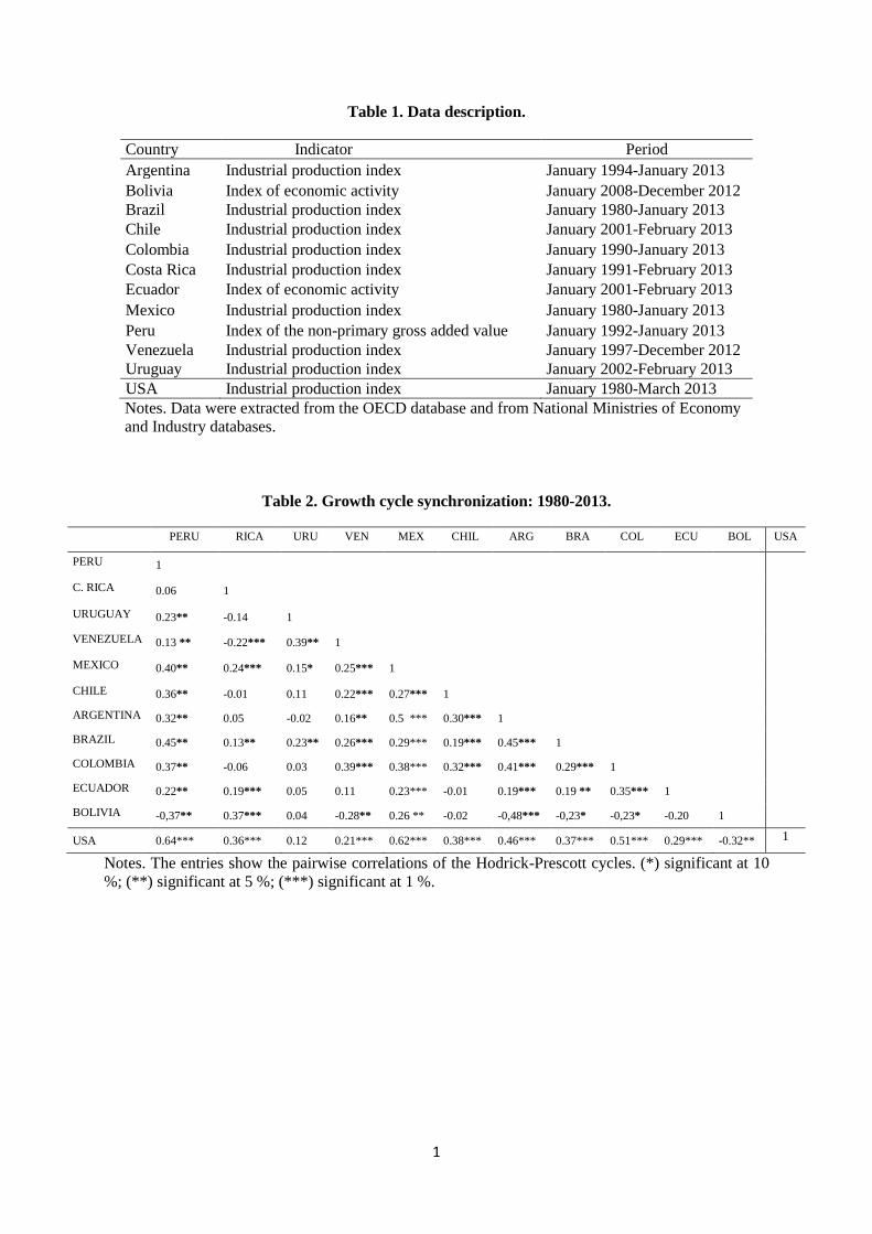
Table 1 shows the variables used in the analysis and the effective sample periods per
country.iv Data were extracted from the OECD database and from National Ministries of
Economy and Industry databases. The time series were filtered with TRAMO-SEATS
and the seasonally adjusted series were analyzed by using the two alternative
approaches: growth cycles and business cycles.
3.1. Results from the growth-cycle analysis
In line with the related literature, the analysis of HP correlations (Table 2) evidences
the existence of significant cyclical links among Latin American countries (77.8% of
the coefficients have statistical significance). In Brazil and Mexico, the largest
economies of the region in terms of GDP, all of the correlation coefficients are
statistically significant. Other distinguished cases are Argentina (80% of significant
correlations), Peru (90%) and Colombia (80%). By contrast, the most desynchronized
nations are Uruguay and Costa Rica, which show relatively lower proportions of
significant coefficients (40% and 50% respectively), and Ecuador and Bolivia, which
show low average ratios (0.13 and -0.16 respectively).
9
By pairs of countries, there is remarkably variety of important associations. The
most important coefficients are those existing between Argentina and Mexico (0.5),
Brazil and Argentina (0.45), Peru and Brazil (0.45), Mexico and Peru (0.40) and
Argentina and Colombia (0.41). Some of these figures can be connected with other
results in the related literature: Mejía-Reyes (1999) detect associations between
Argentina and Brazil and Peru and Brazil, Hurtado-Rendón and Builes-Vásquez (2010)
find similarities between Brazil-Peru, and Aiolfi et al. (2006) obtain significant linkages
between Argentina and Mexico.
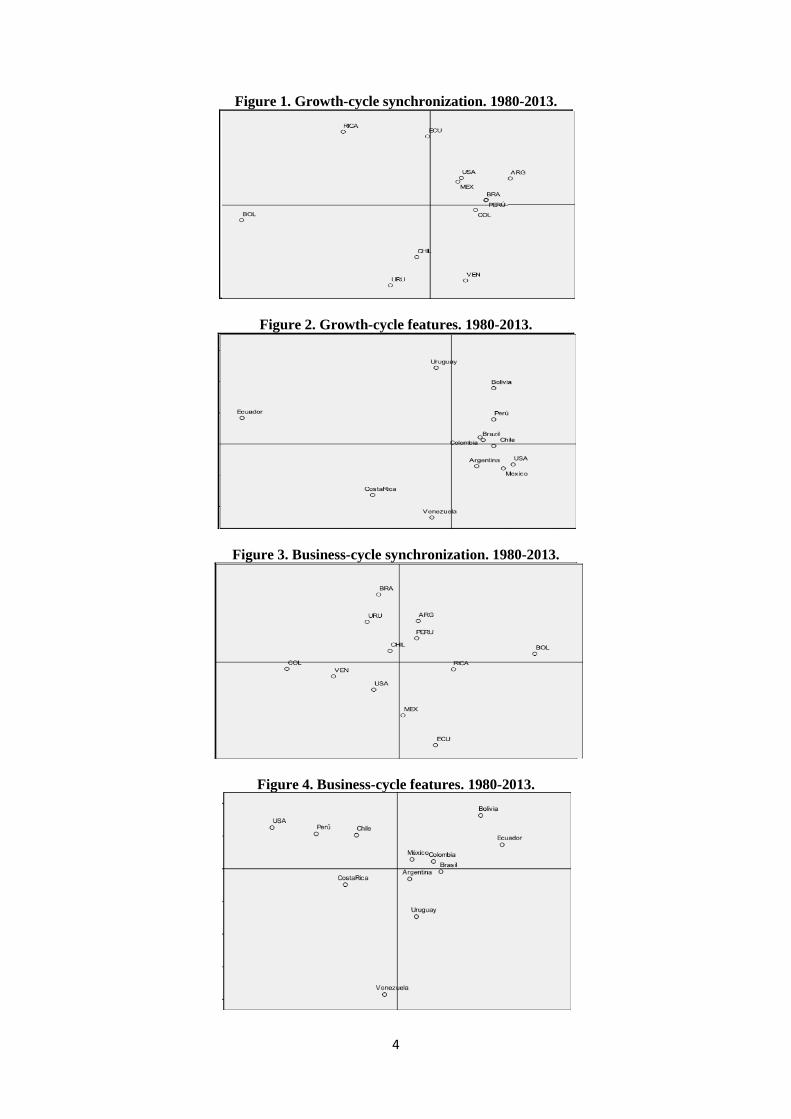
Figure 1 shows the MDS map of growth-cycle synchronization distances over the
sample.v This map clearly reflects the information contained in Table 2. Countries with
the highest degree of growth-cycle synchronization as Brazil, Mexico and Argentina are
represented by points that are closer together in the map. By contrast, countries with
less synchronized cycles as Ecuador (Hurtado-Rendón and Builes-Vásquez, 2010),
Bolivia and Costa Rica are further apart.
Does it mean that this result agrees with a core-periphery interpretation (Artis and
Zhang, 2001) of the growth-cycle synchronization across the Latin American countries?
To evaluate this fact, we examine the number of modes on the distribution of the
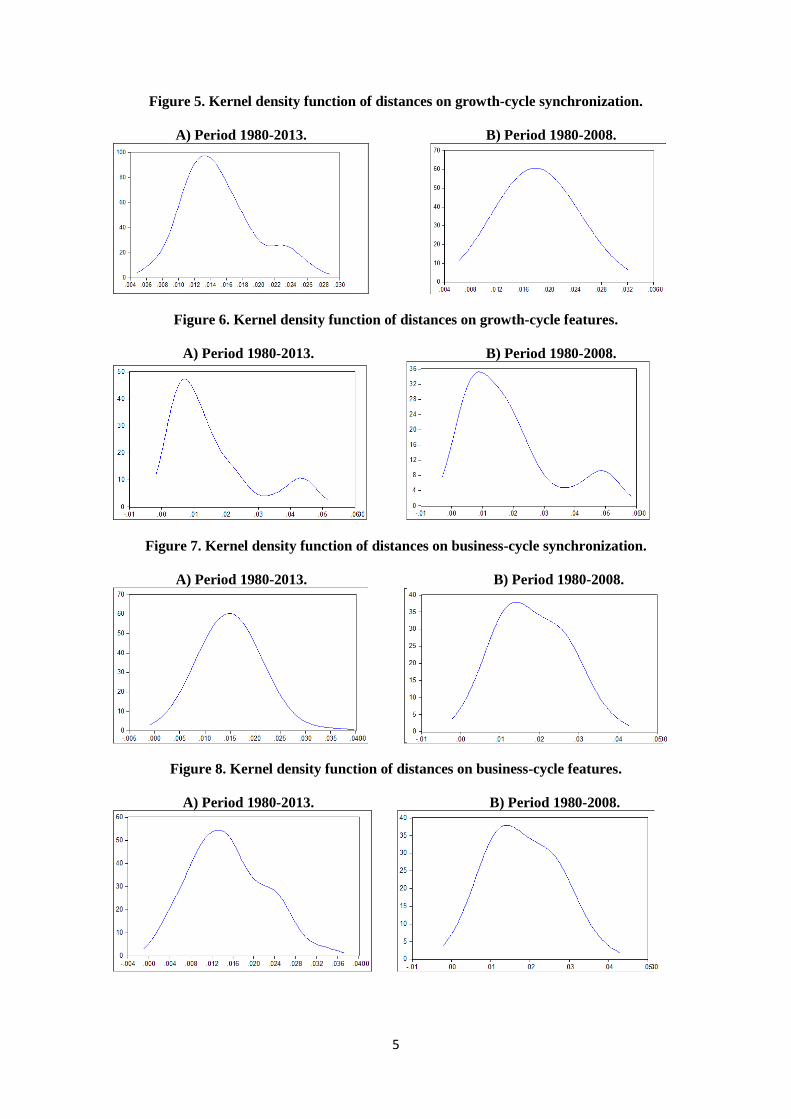
pairwise distances on growth-cycle synchronization that appear in Figure 5. The kernel
density plots of this figure seems to have two modes. The main one is placed around
0.14, indicating that these countries are highly synchronized. In addition, there is a
smaller bump around 0.23 formed by the countries with more idiosyncratic cycles.
By testing for the number of modes in the density probability distribution of the data
(Table 6), we fail to reject the null hypothesis of unimodality. This indicates that, in
spite of the presence of the small bump in the right-hand tail of the distribution, we do
not find different groups of countries in the data in terms of their growth-cycle
synchronization, which does not agree with the core-periphery story.
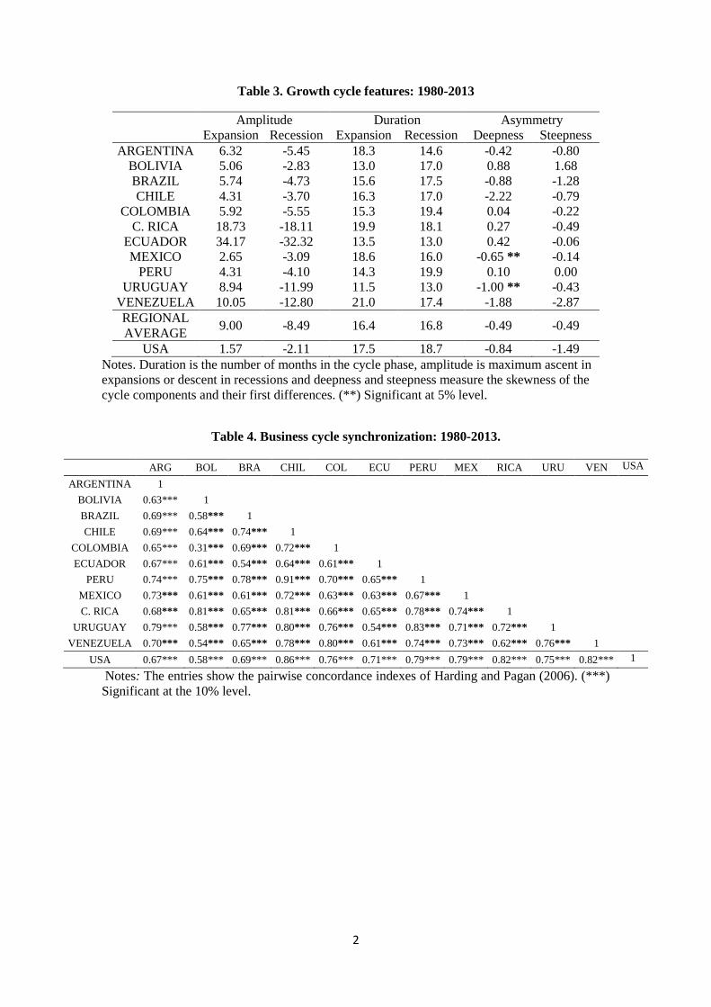
To complete our growth-cycle analysis, we also compute the distance on other
growth-cycle characteristics (amplitude, duration, deepness and steepness). The results,
which are displayed in Table 3, show that the average duration is about 16 months in
both phases of the growth cycle. However, Venezuela and Costa Rica show cycles that
become much longer than the average while Ecuador and Uruguay face the shortest
cycles. There is a small variability in terms of phase durations across countries.
10
Venezuela experienced the longest expansions (21 months) while Uruguay faced the
shortest (11.5 months). Regarding to contractions, Peru present the longest (20 months)
and the shortest belong to Ecuador and Uruguay (13 months).
Amplitude in expansions and recessions is also relatively symmetric. On average,
the maximum ascent of the cycle occurred in expansions is 9, while the maximum
descent in recessions is 8.49. With the exception of three countries (Uruguay,
Venezuela and Mexico), average amplitudes are greater in expansionary phases.
Ecuador, Costa Rica and Venezuela are the countries with the most volatile cycles.
Mexico, Chile, Peru and Bolivia (as in Hurtado-Rendón and Builes-Vásquez, 2010)
experienced the less volatiles cycles during the considered period.
On average, deepness and steepness reach a value of -0.49. This implies that
recessions are deeper than expansions and that the cycle falls rapidly in recessions and
only recovers slowly over time. Chile and Venezuela have the deepest recessions and
Bolivia has the deepest expansion. Bolivia has the steepest expansions and Venezuela
the steepest recessions.
The MDS map of growth-cycle features is reported in Figure 2, which provides a
visual inspection of the relative dissimilarities on the growth-cycle features of Latin
American countries. Notably, the largest countries stick together in the map, reflecting
that these countries form a cluster that shows growth-cycle features that are similar
among them. In addition, some countries are plotted further away from the cluster
formed by the largest countries, which reflects the differences between their cycles and
those of the cluster. These countries also appear separate from each other, which
indicates that their growth-cycle characteristics are idiosyncratic. This group of
countries with idiosyncratic growth cycles is mainly formed by Ecuador, Venezuela,
Costa Rica, Uruguay and, to lesser extent, Bolivia.
Figure 6 shows that bimodality is a visual feature of the kernel estimate of the
distribution of distances on growth-cycle features, measured as the Euclidean distance
across all of the features examined below. It shows that the countries of the cluster
exhibit an average distance on their growth-cycle features of about 0.005 while the
average distance for the countries with idiosyncratic growth-cycles grows up to about
0.05. This bimodal characterization is statistically confirmed by the Silverman test
displayed in Table 6.
11
3.2. Results from the business-cycle analysis
The business cycle synchronization is examined in Table 4. Typically, the pairwise
concordance indexes range between 0.6 and 0.7, which implies that most of the pairs of
Latin American countries crossed through identical business cycle phases between 60%
and 70% of the time elapsed between 1980 and 2013.vi
This evidences their significant
business cycle synchronicity. At the country level, Peru, Chile and Uruguay show the
highest average rates (0.76, 0.75 and 0.73 respectively); while Bolivia (0.61) and
Ecuador (0.62) represent the less synchronized countries.
By pairs of countries, the most important cyclical comovements in terms of
concordance indexes are: Bolivia-Costa Rica (0.81), Chile-Costa Rica (0.81), Chile-
Uruguay (0.80), Colombia-Venezuela (0.80), Peru-Uruguay (0.83) and Chile-Peru
(0.91). In addition, we also find significant comovements in the following pairs of
countries: Uruguay-Argentina (0.79), Bolivia-Peru (0.75), Brazil-Peru (0.78), Brazil-
Uruguay (0.77), Chile-Venezuela (0.78), Colombia-Uruguay (0.76), Peru-Costa Rica
(0.78), as well as Uruguay-Venezuela (0.76). Some of these high values of pairwise
comovements were already found in the literature: Uruguay-Argentina and Uruguay-
Venezuela by Hurtado-Rendón and Builes-Vásquez (2010); Brazil-Uruguay by
Carrasco and Reis (2006); and Brazil-Peru by Hurtado-Rendón and Builes-Vásquez
(2010) and Mejía-Reyes (1999).
Figure 3 shows a graphical representation of the MDS technique, which has been
derived only from the distances on business cycle synchronization. All countries appear
tightly clustered forming only one group. This reveals that the sample of countries is
rather homogeneous in terms of business cycle synchronization.
In line with these uniformly distributed high values of the pairwise concordance
indexes, the kernel representation of the distances on business cycle synchronization
plotted in Figure 7 suggests that the underlying distribution of distances is unimodal.
This suggests that Latin American business cycle cohere. The fact that we fail to find
different sub-populations of Latin American countries is corroborated by the result of
the Silverman test displayed in the third row of Table 6. The p-value of the null of
12
unimodality is 0.41, which implies that this null cannot be rejected at standard
confidence intervals.
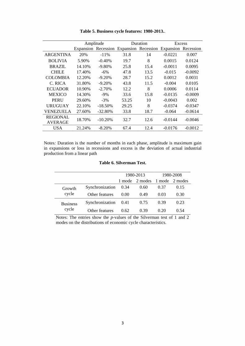
As in the case of growth cycles, we complete our business-cycle analysis by
examining the distance on other business-cycle characteristics in Table 5. In line with
Mejía-Reyes (1999, 2004), we find a large asymmetric behaviour over the business
cycle for most economies in the sample. On average, the duration of the business cycles
implies that expansions last much longer than recessions (duration of 32.7 and 12.6
months, respectively). This asymmetry is remarkable in Peru (53.25 versus 10 months),
Chile (47.8 versus 13.5 months), Costa Rica (43.8 versus 11.5 months) and Uruguay
(29.25 versus 8 months). We also observe a great variability of the full cycle across
countries, something already mentioned by Mejía-Reyes (1999). The duration of
expansions exhibit a huge variability across countries (53.3 months in Peru vs 12.2
months in Ecuador). Moreover, the duration of recessions is relatively similar across
nations (18.7 months in Venezuela vs 8 months in Bolivia, Ecuador and Uruguay).
These findings also appear in Calderón and Fuentes (2010).
On average, the gains in expansions are about 18.7% while the losses in recessions
are of 10.2%. Again, the well-known high volatility of the Latin American cycles is
remarkable (see, among others, Aiolfi et al., 2006, and Mejía-Reyes 1999 and 2004).
Moreover, the variability in the amplitude of the Latin American business cycles is
noticeable, in line with the findings of Calderón and Fuentes (2010). Costa Rica is the
nation with the highest increase of its industrial production in times of economic growth
(31.8%), followed by Peru (29.6 %), Venezuela (27.6 %) and Uruguay (22.1 %). By
contrast, Venezuela (-32.8 %) and Uruguay (-18.5 %) are the countries with the largest
falls of industrial product during economic downturns. This singularity places these
countries as those with the most volatile cycles. In contrast to these countries, Bolivia
show the less volatile business cycle.
Overall, Latin American countries exhibit negative excess in expansions and
positive excess in recessions. Therefore, industrial production increases in expansions
intensively after the troughs (Bolivia, Ecuador and Colombia are the only exceptions).
By contrast, industrial production falls quickly after the peaks during recessions (Chile,
México, Uruguay and Venezuela are the exceptions).
13
The MDS map displayed in Figure 4 greatly helps in the comparison of all the
distances in business-cycle features. According with this representation, the countries
are grouped in two concentric circles, whose radius lengths reflect the business cycle
dissimilarities from the centre to the periphery. The core of countries with more similar
business cycles are Argentina, Mexico, Brazil, Uruguay Colombia and C. Rica.
Ecuador, Bolivia Venezuela, Peru and Chile are located in the periphery
The kernel approximation to the density distribution of distances in business-cycle
features is plotted in Figure 8. The density estimation suggests that the countries with
more homogeneous business cycles belong to the mass of the distribution. The smaller
bump placed in the right-hand-side tail of the distribution refer to those countries with
more heterogeneous business cycles. In spite of this comment, the Silverman test
displayed in Table 6 fails to find two different modes in the distribution of distances in
business-cycle features since the p-value of the null of one mode is 0.62.
3.3. Economic cycle structures and dynamic evolution
In the previous sections we show that regardless of the approach used to compute
the cycle features, we find evidence of significant linkages in this region. With the
exception of the growth cycle features, the Latin American countries exhibited pretty
similar cycles during this sample period. This result is of significant importance for the
economic integrations that are currently being implemented in the region.
In this context, some results in the recent literature point out that part of the cyclical
linkages may rely on presence of the Great Recession. Imbs (2010) argues that world
synchronization has greatly increased due to the Great Recession, mainly due to the
linkages observed among developed countries. In addition, Fidrmuc and Korhonen
(2010) finds that the rises in synchronization have been particularly important between
the largest Asian emerging economies (China and India) and the industrialized
countries. However, Gächter et al. (2012) show a pronounced desynchronization of
business cycles in Economic and Monetary Union during the crisis period, both with
respect to dispersion and to the correlation of business cycles.
Although there are some studies (for example, Hurtado-Rendón and Builes-
Vásquez, 2010) that focus on the reinforcements of the cyclical links in the region in
14
periods of instability (in the “lost decade” and the last years of the previous century),
they do not cover the Great Recession, or only the initial years of the same. The purpose
of this section is to examine the extent to which the economic cycle linkages in Latin
American countries documented above were affected by the Great Recession.
For this purpose, we examine the dynamic of the density distributions of pairwise
economic cycle distances by repeating the analysis with sample that ends before the
Great Recession. According to Figure 5 to Figure 8, the modes slightly shifts to the left
when the data of the Great Recession are included in the sample, especially in the case
of growth cycle and business cycle synchronization. This agrees with the view that the
business cycles of individual countries may have become more closely synchronized
because the Latin American countries experienced the effects of this recession roughly
at the same time.
The last two column of Table 6 show the p-values of the null of testing for the
number of modes in the density probability distribution of the data when the sample
ends in 2007. The table shows that we have virtually identical results regardless of
whether the data of the Great Recession are included in the sample. As in the case of the
entire sample, the unimodality hypothesis is not rejected in the case of growth-cycle
synchronization, business-cycle synchronization and business-cycle features. In
addition, the distribution of growth-cycle features seems to have two modes. Therefore,
it seems that the Great Recession did not have significant effects on the pre-existing
Latin American cyclical linkages.vii
4. CONCLUDING REMARKS
The main conclusions about the situation of Latin American cycles during the last
thirty years can be summarized as follows. First, regardless of the approach used to
compute the cycle features, we find evidence of significant linkages in this region.
Second, the growth-cycle features tend to be more symmetric across the cycle than the
business cycle features. Third, the Great Recession did not lead to any significant
impact on the Latin American distribution of distances on economic cycles. Moreover,
except for the growth cycle features for which we find two modes in the distribution of
distances, Latin America countries had pretty uniform cycles in this period. In spite of
15
this comment, we find that the countries with more idiosyncratic cycles are Bolivia,
Ecuador and Costa Rica.
These results are of significant importance for the economic integrations that are
currently being implemented in the region. With few exceptions, we find that Latin
American countries exhibit similar cycles during the sample period. Therefore, we think
that the cyclical synchronization and the similarities on other cycle characteristics
would not be an obstacle to follow with the economic integrations already initiated
among some of these countries.
16
REFERENCES
Artis, M. J. and W. Zhang. "Core and periphery in EMU: A cluster analysis."
Economic Issues Journal Articles 6, no. 2 (2001): 47-58.
Boschan, C. and G. Bry. “Cyclical Analysis of Time Series: Selected Procedures
and Computer Programs.” National Bureau of Economic Research, 1971.
Calderón, C. and R. Fuentes. "Characterizing the Business Cycles of Emerging
Economies." World Bank Policy Research Working Paper Series, Vol (June 2010).
Camacho, M.; G. Perez-Quiros; and L. Saiz. "Are European Business Cycles Close
Enough to Be Just One?" Journal of Economic Dynamics and Control 30, no. 9
(October 2006): 1687-706.
Camacho, M.; G. Perez-Quiros; and L. Saiz. "Do European Business Cycles Look
Like One?" Journal of Economic Dynamics and Control 32, no. 7 (July 2008): 2165-90.
Christodoulakis, N.; S. Dimelis; and T. Kollintzas. "Comparisons of Business
Cycles in the Ec: Idiosyncracies and Regularities." Economica (February 1995): 1-27.
De Haan, J.; R. Inklaar; and R. Jong‐A‐Pin. "Will Business Cycles in the Euro Area
Converge? A Critical Survey of Empirical Research." Journal of economic surveys 22,
no. 2 (April 2008): 234-73.
Fidrmuc, J. and I. Korhonen. "The Impact of the Global Financial Crisis on Business
Cycles in Asian Emerging Economies." Journal of Asian Economics 21, no. 3 (June
2010): 293-303.
Gächter, M.; A. Riedl; and D. Ritzberger-Grünwald. "Business Cycle
Synchronization in the Euro Area and the Impact of the Financial Crisis." Monetary
Policy & The Economy, Quarterly Review of Economic Policy, Oesterreichische
Nationalbank Q 2 (May 2012): 33-60.
Carrasco, C. E. and F. A. Reis. "Evidence About Mercosur’s Business Cycle." Paper
presented at the Anais do XXXIV Encontro Nacional de Economia [Proceedings of the
34th Brazilian Economics Meeting], no. 179, October 2006.
17
Harding, D. and A. Pagan. "Dissecting the Cycle: A Methodological Investigation."
Journal of monetary economics 49, no. 2 (March 2002): 365-81.
Hodrick, R. J and E. C. Prescott. "Postwar Us Business Cycles: An Empirical
Investigation." Journal of Money, credit, and Banking (February 1997): 1-16.
Iguíñiz, J. and G. Aguilar. ''Ciclos Peruanos, Andinos y de Estados Unidos''. Revista
del departamento de economía de la Pontificia Universidad Católica del Perú 20, no.
39-40 (1998): 165-206.
Imbs, Jean. "The First Global Recession in Decades." IMF economic review 58, no.
2 (December 2010): 327-54.
Mejía-Reyes, Pablo. "Classical Business Cycles in Latin America: Turning Points,
Asymmetries and International Synchronization." Estudios Económicos 14, no. 2 (July
1999): 265-97.
Mejía-Reyes, Pablo. "Classical Business Cycles in America: Are National Business
Cycles Synchronised?" International Journal of Applied Econometrics and Quantitative
Studies 1, no. 3 (2004): 75-102.
Rendón, A. and F. Builes-Vásquez. "Sincronización de Ciclos Económicos en el
Mercosur: 1960-2008." Ecos de Economía 14, no. 31 (July 2010).
Sichel, Daniel. "Business Cycle Asymmetry: A Deeper Look." Economic Inquiry
31, no. 2 (April 1993): 224-36.
Silverman, Bernard. "Using Kernel Density Estimates to Investigate
Multimodality." Journal of the Royal Statistical Society. Series B (Methodological)
(January 1981): 97-99.
Stock, J. H. and M. W. Watson. "Estimating Turning Points Using Large Data
Sets." Journal of Econometrics 178 (January 2014): 368-81.
Timmermann, A.; L. Catão; and M. Aiolfi. Common Factors in Latin America's
Business Cycles. International Monetary Fund, February 2006.
Timm, Neill. Applied Multivariate Analysis. Berlin: Springer Texts in Statistics,
2002.
18
NOTES
i In particular, we implement the Bry-Boschan Gauss code created for Stock and
Watson (2014).
ii A good reference on MDS techniques is Timm (2002).
iii Following the suggestion of the reviewers, we repeated all the analyses developed in
the paper using GDP. Although the results are omitted to save space (they are available
upon request) they are qualitatively similar to those that we obtained with IP.
iv Due to data availability problems, we use the index of economic activity for Bolivia
and Ecuador and the non-primary added value index for Peru.
v In these maps, the axes are meaningless and the orientation of the picture is arbitrary.
vi All the indexes in the table are statistically significant.
vii Following the suggestion of a reviewer, we repeated all the analyses developed in the
paper using the year 2000 as the breakpoint. Although the results are omitted to save
space (they are available upon request) they are qualitatively similar to those that using
2008 as the breakpoint.
1
Table 1. Data description.
Country Indicator Period
Argentina Industrial production index January 1994-January 2013
Bolivia Index of economic activity January 2008-December 2012
Brazil Industrial production index January 1980-January 2013
Chile Industrial production index January 2001-February 2013
Colombia Industrial production index January 1990-January 2013
Costa Rica Industrial production index January 1991-February 2013
Ecuador Index of economic activity January 2001-February 2013
Mexico Industrial production index January 1980-January 2013
Peru Index of the non-primary gross added value January 1992-January 2013
Venezuela Industrial production index January 1997-December 2012
Uruguay Industrial production index January 2002-February 2013
USA Industrial production index January 1980-March 2013
Notes. Data were extracted from the OECD database and from National Ministries of Economy
and Industry databases.
Table 2. Growth cycle synchronization: 1980-2013.
PERU RICA URU VEN MEX CHIL ARG BRA COL ECU BOL USA
PERU 1
C. RICA 0.06 1
URUGUAY 0.23** -0.14 1
VENEZUELA 0.13 ** -0.22*** 0.39** 1
MEXICO 0.40** 0.24*** 0.15* 0.25*** 1
CHILE 0.36** -0.01 0.11 0.22*** 0.27*** 1
ARGENTINA 0.32** 0.05 -0.02 0.16** 0.5 *** 0.30*** 1
BRAZIL 0.45** 0.13** 0.23** 0.26*** 0.29*** 0.19*** 0.45*** 1
COLOMBIA 0.37** -0.06 0.03 0.39*** 0.38*** 0.32*** 0.41*** 0.29*** 1
ECUADOR 0.22** 0.19*** 0.05 0.11 0.23*** -0.01 0.19*** 0.19 ** 0.35*** 1
BOLIVIA -0,37** 0.37*** 0.04 -0.28** 0.26 ** -0.02 -0,48*** -0,23* -0,23* -0.20 1
USA 0.64*** 0.36*** 0.12 0.21*** 0.62*** 0.38*** 0.46*** 0.37*** 0.51*** 0.29*** -0.32** 1
Notes. The entries show the pairwise correlations of the Hodrick-Prescott cycles. (*) significant at 10
%; (**) significant at 5 %; (***) significant at 1 %.
2
Table 3. Growth cycle features: 1980-2013
Amplitude Duration Asymmetry
Expansion Recession Expansion Recession Deepness Steepness
ARGENTINA 6.32 -5.45 18.3 14.6 -0.42 -0.80
BOLIVIA 5.06 -2.83 13.0 17.0 0.88 1.68
BRAZIL 5.74 -4.73 15.6 17.5 -0.88 -1.28
CHILE 4.31 -3.70 16.3 17.0 -2.22 -0.79
COLOMBIA 5.92 -5.55 15.3 19.4 0.04 -0.22
C. RICA 18.73 -18.11 19.9 18.1 0.27 -0.49
ECUADOR 34.17 -32.32 13.5 13.0 0.42 -0.06
MEXICO 2.65 -3.09 18.6 16.0 -0.65 ** -0.14
PERU 4.31 -4.10 14.3 19.9 0.10 0.00
URUGUAY 8.94 -11.99 11.5 13.0 -1.00 ** -0.43
VENEZUELA 10.05 -12.80 21.0 17.4 -1.88 -2.87
REGIONAL
AVERAGE 9.00 -8.49 16.4 16.8 -0.49 -0.49
USA 1.57 -2.11 17.5 18.7 -0.84 -1.49
Notes. Duration is the number of months in the cycle phase, amplitude is maximum ascent in
expansions or descent in recessions and deepness and steepness measure the skewness of the
cycle components and their first differences. (**) Significant at 5% level.
Table 4. Business cycle synchronization: 1980-2013.
ARG BOL BRA CHIL COL ECU PERU MEX RICA URU VEN USA
ARGENTINA 1
BOLIVIA 0.63*** 1
BRAZIL 0.69*** 0.58*** 1
CHILE 0.69*** 0.64*** 0.74*** 1
COLOMBIA 0.65*** 0.31*** 0.69*** 0.72*** 1
ECUADOR 0.67*** 0.61*** 0.54*** 0.64*** 0.61*** 1
PERU 0.74*** 0.75*** 0.78*** 0.91*** 0.70*** 0.65*** 1
MEXICO 0.73*** 0.61*** 0.61*** 0.72*** 0.63*** 0.63*** 0.67*** 1
C. RICA 0.68*** 0.81*** 0.65*** 0.81*** 0.66*** 0.65*** 0.78*** 0.74*** 1
URUGUAY 0.79*** 0.58*** 0.77*** 0.80*** 0.76*** 0.54*** 0.83*** 0.71*** 0.72*** 1
VENEZUELA 0.70*** 0.54*** 0.65*** 0.78*** 0.80*** 0.61*** 0.74*** 0.73*** 0.62*** 0.76*** 1
USA 0.67*** 0.58*** 0.69*** 0.86*** 0.76*** 0.71*** 0.79*** 0.79*** 0.82*** 0.75*** 0.82*** 1
Notes: The entries show the pairwise concordance indexes of Harding and Pagan (2006). (***)
Significant at the 10% level.
3
Table 5. Business cycle features: 1980-2013..
Amplitude Duration Excess
Expansion Recession Expansion Recession Expansion Recession
ARGENTINA 20% -11% 31.8 14 -0.0221 0.007
BOLIVIA 5.90% -0.40% 19.7 8 0.0015 0.0124
BRAZIL 14.10% -9.80% 25.8 15.4 -0.0011 0.0095
CHILE 17.40% -6% 47.8 13.5 -0.015 -0.0092
COLOMBIA 12.20% -9.20% 28.7 15.2 0.0012 0.0031
C. RICA 31.80% -9.20% 43.8 11.5 -0.004 0.0105
ECUADOR 10.90% -2.70% 12.2 8 0.0006 0.0114
MEXICO 14.30% -9% 33.6 15.8 -0.0135 -0.0009
PERU 29.60% -3% 53.25 10 -0.0043 0.002
URUGUAY 22.10% -18.50% 29.25 8 -0.0374 -0.0347
VENEZUELA 27.60% -32.80% 33.8 18.7 -0.064 -0.0614
REGIONAL
AVERAGE 18.70% -10.20% 32.7 12.6 -0.0144 -0.0046
USA 21.24% -8.20% 67.4 12.4 -0.0176 -0.0012
Notes: Duration is the number of months in each phase, amplitude is maximum gain
in expansions or loss in recessions and excess is the deviation of actual industrial
production from a linear path
Table 6. Silverman Test.
1980-2013 1980-2008
1 mode 2 modes 1 mode 2 modes
Growth
cycle
Synchronization 0.34 0.60 0.37 0.15
Other features 0.00 0.49 0.03 0.30
Business
cycle
Synchronization 0.41 0.75 0.39 0.23
Other features 0.62 0.39 0.20 0.54
Notes: The entries show the p-values of the Silverman test of 1 and 2
modes on the distributions of economic cycle characteristics.
4
Figure 1. Growth-cycle synchronization. 1980-2013.
Figure 2. Growth-cycle features. 1980-2013.
Figure 3. Business-cycle synchronization. 1980-2013.
Figure 4. Business-cycle features. 1980-2013.
5
Figure 5. Kernel density function of distances on growth-cycle synchronization.
A) Period 1980-2013. B) Period 1980-2008.
Figure 6. Kernel density function of distances on growth-cycle features.
A) Period 1980-2013. B) Period 1980-2008.
Figure 7. Kernel density function of distances on business-cycle synchronization.
A) Period 1980-2013. B) Period 1980-2008.
Figure 8. Kernel density function of distances on business-cycle features.
A) Period 1980-2013. B) Period 1980-2008.