Lateral Model Predictive Controlfor Over-Actuated Autonomous Vehicle

Goncalo Collares Pereira1, Lars Svensson2, Pedro F. Lima3, Jonas Martensson3

Abstract— In this paper, a lateral controller is proposed foran over-actuated vehicle. The controller is formulated as alinear time-varying model predictive controller. The aim of thecontroller is to track a desired path smoothly, by making useof the vehicle crabbing capability (sideways movement) andminimizing the magnitude of curvature used. To do this, notonly the error to the path is minimized, but also the errorto the desired orientation and the control signals requests.The controller uses an extended kinematic model that takesinto consideration the vehicle crabbing capability and is ableto track not only kinematically feasible paths, but also planand track over non-feasible discontinuous paths. Ackermannsteering geometry is used to transform the control requests,curvature, and crabbing angle, to wheel angles. Finally, thecontroller performance is evaluated first by simulation and,after, by means of experimental tests on an over-actuatedautonomous research vehicle.

I. INTRODUCTION

The increased demand for transportation lead to an in-crease in traffic congestions. Traffic congestion is in turnassociated with decreased productivity, increased numberof accidents as well as increased air pollution, and energyconsumption [1], [2]. Autonomous vehicles present oppor-tunities to mitigate these problems. In the past few years,many major vehicle manufacturers have been increasing theirresearch in the field of autonomous vehicles and the firstcommercialized autonomous vehicle are already out on theroads. Autonomous driving is not a new idea and it wastested and proven possible in different competitions, such asDARPA grand and urban challenges [3], [4].

There are many different challenges associated with au-tonomous vehicles. A central technical challenge is lateralcontrol of the vehicle. Where as the majority of research anddevelopment focuses on the most common 2 wheel-steering(2WS) configuration [5], [6], this paper deals with the pathtracking problem for a 4 wheel-steered vehicle (4WS).

For many years, we have seen examples of 4 wheelsteering vehicles in adjacent domains, such as constructionvehicles and field robotics [7]. Interesting examples canalso be found inthe automotive domain, such as, the DLRRobomobil [8] and the Stanford VAIL experimental vehicles[9] have been around for some time, and, recently, we haveseen more examples also from industry, such as the Easymile4-wheel steering autonomous shuttle [10].

1Integrated Transport Research Lab, Department of Automatic Con-trol, KTH Royal Institute of Technology, SE-100 44 Stockholm, Sweden.gpcp@kth.se

2Integrated Transport Research Lab, Department of Machine Design,KTH Royal Institute of Technology, SE-100 44 Stockholm, Sweden.larsvens@kth.se

3Integrated Transport Research Lab and ACCESS Linnaeus Centre,Department of Automatic Control, KTH Royal Institute of Technology, SE-100 44 Stockholm, Sweden. pfrdal@kth.se jonas1@kth.se

Fig. 1: Research concept vehicle (RCV).

A motivation for introducing 4WS is that it can improveyaw stability at high speed as well as manoeuvrability atlow speed, as argued by Sano et al in [11]. Furthermore,4WS allows for a type of motion called crabbing, wherethe vehicle moves diagonally sideways. For example, thecrabbing capability of the vehicle can be used to performlane change maneuvers with minimal yaw rate or parallelparking in tight spaces.

However, control strategies presented in literature for4WS vehicles are usually based on thorough knowledge ofvehicle dynamics and rudimentary PID control. We arguethat applying model predictive control for path trackingcontrol of a 4WS vehicle is a novel concept that can improvepath tracking performance while maintaining a smooth andcomfortable ride.

Fig. 1 presents the vehicle used for implementation andtesting. The research concept vehicle (RCV) is an experi-mental and research platform built at KTH Royal Instituteof Technology at the Integrated Transport Research Lab(ITRL) [12]. This vehicle is able to steer all four wheelsindependently [13].

Model predictive control (MPC) has been widely used tosolve the lateral control problem of autonomous vehicles,e.g., [5], [6], [14], [15]. In [5], a MPC controller computesthe front steering angle in order to follow a trajectory onslippery roads at the highest possible entry speed. There, anonlinear MPC (NMPC) is implemented but, because of thecomputational burden, experimental tests could only be madeat low entry speeds. To reduce the complexity of the problem,an alternative approach is presented based on successive on-line linearization of the vehicle model. A linear time-varyingMPC (LTV-MPC) is implemented and tested, proving thatthe controller is able to stabilize the vehicle with a speedof up to 21 m/s on slippery surfaces. In [6], a LTV-MPCapproach is used to overcome obstacles on the road and keep

2017 IEEE Intelligent Vehicles Symposium (IV)June 11-14, 2017, Redondo Beach, CA, USA

978-1-5090-4804-5/17/$31.00 ©2017 IEEE 310

the lane. The controller is able to avoid obstacles with anentry speed of approximately 14 m/s. There, the longitudinaland lateral control problem is separated into different opti-mization problems, which helps reducing the computationalcost. In [14], an MPC based controller is used to stabilizea vehicle along a desired path while rejecting wind gustsand, on another scenario, perform double lane changes. Itis able to stabilize the vehicle up to side wind speeds of10.1 m/s on the wind rejection scenario and 17 m/s of entryspeed in the double lane change maneuvers. However, due tothe computational complexity of the feedback control policy,not all results are experimentally validated. More recently in[15], an LTV-MPC is used to obtain smooth and accuratepath following. The optimization cost function introducesthe idea of trade off between smoothness and accuracy whenfollowing a path, making use of the available free space (e.g.,lane width). The controller is experimentally evaluated in aScania mining truck and the results show that the controlleris able to maintain the vehicle within 15 cm of the referencepath both in high and low speeds.

MPC performance is highly influenced by the model used.Different models lead to different problem complexities,which ultimately lead to different computation times. In[16], kinematic and dynamic vehicle models are studiedto motivate an MPC controller. The results show that thekinematic model discretized at 200 ms is able to perform aswell as a dynamic model discretized at 100 ms. Therefore,the authors propose MPC design based on the kinematicmodel instead of a higher fidelity model. In [17], differentvehicle models for lateral vehicle dynamics are described,which are then used by the author to develop and validatecontrollers to maintain a vehicle in the center of its road laneboundaries.

The work presented in this paper extends the previousresearch. A kinematic vehicle model is extended to takeinto consideration the extra degree of freedom of the RCVand used to design an LTV-MPC for lateral control of thevehicle. The controller makes use of crabbing angle andcurvature requests to follow a desired path in a smooth andcomfortable manner. Furthermore, the controller is subject toa two-phase validation. First, the controller is validated in asimulation environment that uses an accurate vehicle modelof the RCV. Then, the controller is implemented in the RCVand its performance evaluated through field tests at a localtest site at KTH, Stockholm, Sweden.

This paper is organized as follows: in Section II, the vehi-cle’s steering concept is presented; in Section III, the vehiclemodels used are presented; in Section IV, the problem ofpath following is addressed by developing an LTV-MPCcontroller; in Section V, both simulation and experimentalresults are presented and compared; finally, in Section VI,concluding remarks are presented and future work outlined.

II. STEERING CONCEPT

Ackerman steering is a geometric arrangement for mini-mizing tire slip when a vehicle is turning. This is achievedby choosing steering angles such that all wheels are tangentto a set of concentric circles. Assuming planar motion andsmall tire slip, the vehicle rotates about the center of the

lf

PR

R

δfl

γfl

β

lr

β

dflλfl

Fig. 2: Geometric relations between δfl and point of rotation,PR.

circle, called the instantaneous center of rotation PR, i.e.,the vehicle turns with the curvature κ = 1/R, where R isthe distance between the rotational center of the vehicle andPR.

For 2WS vehicles, PR must be placed on a line thatextends the rear axle, but for 4WS vehicles, it can be placedat an arbitrary point in the plane, provided that steering angleconstraints for each individual wheel are respected. PlacingPR in front or behind the point of rotation causes the vehicleto crab, thus introducing an additional degree of freedom.PR is expressed in polar coordinates in the vehicle frame,

see Fig. 2. The argument β corresponds to the angle betweenthe vehicle’s velocity vector and the forward direction of thevehicle chassis, i.e., the crab angle.

Based on a requested curvature κ and a requested crabbingangle β, PR is fully determined, and from basic trigonometry,the individual steering angles are obtained. For example, thefront left wheel angle δfl = β + γfl, where

γfl = atan

(dflcos(λfl − β)

R− dflsin(λfl − β)

).

Using this formulation, the vehicle is able to crab and curvesimultaneously, while maintaining the Ackerman steeringgeometry.

III. MODELLING

In this section, two different vehicle models are presented.Namely, an extended kinematic model used for vehicleprediction within the MPC framework, and a more complexand accurate dynamic vehicle model for controller validationin simulation.

A. Controller Vehicle Model

The continuous-time differential equations of the vehiclemodel can be obtained by adding the crabbing angle to astandard kinematic model. The vehicle model discretized

311

version is

Xi+1 = Xi + Tsvi cos (Ψi + βi) ,Yi+1 = Yi + Tsvi sin (Ψi + βi) ,Ψi+1 = Ψi + Tsviκi,

(1)

where, X , Y , and Ψ are the vehicle’s coordinates andorientation, respectively, in the world frame, v is the vehiclevelocity, Ts is a sampling time, and β and κ are the controlsignals, crabbing angle and curvature, respectively. The indexi denotes the time instant at which the variable is beingconsidered.

From (1), it is possible to rotate and translate the statesto local vehicle coordinates, i.e., the origin of the Cartesianframe corresponds to the center of gravity pose of the vehicle,and write the vehicle model states as z = [x, y, ψ]

T , andthe control signals as u = [κ, β]

T . As mentioned before,this model is used to predict the vehicle motion in theMPC framework for path following. Since the vehicle modelis clearly nonlinear, it is linearized considering a refer-ence path composed of N points, zref

j =[xrefj ; yref

j ;ψrefj

]and uref

j =[κrefj ;βref

j

], where, j = 1, . . . , N . The reference

points are discretized according to the velocity profile and thesampling time. Finally, the linearized vehicle model states,can be expressed as

zj = Aj zj +Bj uj , (2)

where, zj = zj − zrefj , uj = uj − uref

j , and Aj and Bj canbe expressed as

Aj =

1 0 −Tsvrefj sin

(ψrefj + βref

j

)0 1 Tsv

refj cos

(ψrefj + βref

j

)0 0 1

, (3)

Bj =

0 −Tsvrefj sin

(ψrefj + βref

j

)0 Tsv

refj cos

(ψrefj + βref

j

)Tsv

refj 0

. (4)

B. Simulation Vehicle Model

The vehicle model used in simulation is based upon themodels used in [5], [14], [16], [17] and can be obtained fromFig. 3,

Xi+1 = Xi + Ts(vxicos(Ψi)− vyi sin(Ψi)),

Yi+1 = Yi + Ts(vxisin(Ψi) + vyi cos(Ψi)),

Ψi+1 = Ψi + Tsωi,

vxi+1= vxi

+ Ts

(Fxi

−Fr−Fai

M + vyiωi

),

vyi+1= vyi + Ts

(Fyi

M − vxiωi

),

ωi+1 = ωi + Tslf(F fr

yi+F fl

yi)−lr(F rr

yi+F rl

yi)

I .

(5)

where, vx and vy are the vehicle’s longitudinal and lateralvelocities, in the vehicle’s local frame, ω is the yaw rateof the vehicle, M = m+mI is the total mass, where,m is the vehicle mass and mI is the equivalent massof rotating parts due to inertia, I is the vehicle inertiaaround the z-axis, and lf and lr are the distances fromthe front and rear wheels to the center of gravity (CoG),respectively. The index i denotes the discrete time instantat which the variable is being considered. Without consid-ering the time instant, Fx = F frx + F flx + F rrx + F rlx and

δfr

αfr

F frl

F frcvfrc

vfrl

vfr

lf

lr x

y

ψ

Y

Ψ X

δfl

δrl

δrr

F flc

F fll

F rrcF rrl

F rlc

F rll

Fig. 3: Illustration of the vehicle model used in simulation.The wheels are presented in gray, the forces on each wheelin blue, the velocities for the front right wheel are presentedin green, and the center of gravity and the axis for the localframe of the vehicle are presented in red.

Fy = F fry + F fly + F rry + F rly are the longitudinal and lat-eral forces acting on CoG of the vehicle, Fa = 1

2ρCdAfv2x

is the air drag force, where, ρ is the mass density of air, Cdis the aerodynamic drag coefficient, Af is the frontal areaof the vehicle and, finally, Fr = frollmg cos(θ) is the rollingresistance force, where, froll is the roll resistance coefficient,g is the gravitational acceleration and θ is the road inclinationangle. The notation (.)fr,fl,rr,rl corresponds, respectively, tofront right, front left, rear right, and rear left wheel.

For all wheels a constant normal tire load is assumed, i.e.,Fz = constant. The forces acting on the CoG due to the frontright wheel are

F frx =F frl cos(δfr)− F frc sin(δfr), (6)

F fry =F frl sin(δfr)− F frc cos(δfr), (7)

where, δ is the angle of the wheel, Fl = Tr is the longitudinal

force, where T is the torque and r is the radius, and Fc = Cαis the lateral force of the tire, where C is the corneringstiffness and α is the slip angle that can be expressed forthe front and rear wheels as

αfr,fl =δfr,fl − arctan(vy + lfr,flω

vx), (8)

αrr,rl =δrr,rl − arctan(vy − lrr,rlω

vx). (9)

IV. MODEL PREDICTIVE CONTROLLER

This section addresses the problem of path following fora 4WS vehicle. An LTV-MPC is formulated to perform pathtracking while maintaining a smooth and comfortable ride bymaking use of the additional degree of freedom, the crabbingangle.

The main objective of the controller is to follow a givenpath, even if the path is not planned with a 4WS vehicledynamics in mind. Therefore, the problem of referencegeneration needs to be addressed.

312

A. Reference GenerationThe generation of the reference path points and control

signals is a crucial step, because the linearized vehicle modelis only valid in the vicinity of the linearization points and ishighly dependent on their choice. Furthermore, a good choiceof the reference control signals and path points contributes toa faster convergence of the solver and a smaller computationtime.

Before explaining the reference generation, it is importantto define and introduce some terms. Vehicle orientation isdefined as the yaw (Ψ) of the vehicle. Road direction isdefined by the tangent of the road at any given point.For example, the orientation of a regular vehicle whenperforming a lane change on a straight road does not matchthe path direction, it matches the tangent of the traveled path.

Assuming the path was generated for a regular vehicle,the expected orientation (Ψ) at each point corresponds to thedirection of movement of the vehicle. So, this type of pathdoes not explicitly use the extra degree of freedom β and,if no further information is provided, this term is only usedto correct error and deal with unfeasible paths. However,if the road/desired direction is given to the controller, thedesired orientation at each point becomes the direction ofthe road, which ultimately leads to a smoother and morecomfortable ride, because the vehicle follows the path using acombination of curvature and crabbing, and not, for example,using only curvature to perform a lane change.

Independently of receiving the road direction or not, thereference control signals are constrained to limit values. Theconstrained path

(zref

calc

)is created by trying to follow as

much as possible the direction of the original path(zref

true

),

which in the case presented in Fig. 4 leads to maximumcurvature at the beginning of the step, because during thestep the path direction is π/2 radians, and, then, minimumcurvature to get the direction back to 0 radians to match thepath.

To resume, the original path (zref ) is in the world frameand is used to compute the current error to the path (z), notethat the controller controls over a local frame not the worldframe. So, zref is transformed for the controller into zref

true,which is the original path in local frame coordinates anddiscretized properly taking in consideration the control hori-zon. From zref

true and the reference control signals required tofollow that path, zref

calc is created by constraining the controlsignals.

Limiting the control signals, makes the reference pathpoints feasible, allowing for a faster convergence of thesolver, since the reference points always respect the maxi-mum and minimum control signals constraints. On the otherhand, saturating the control signals, has the disadvantage ofchanging the reference path points, which ultimately wouldmake the vehicle follow a path that is different from theoriginal path. To deal with this, the cost function is modifiedto account for future predicted error, which is presented inFig. 4. In other words, a term is added to the cost functionto account for the difference between the desired path sentto the controller and the reference path used to linearizethe vehicle model. This is further explained in the nextsubsection.

Y

ΨX

x

y

ψ

Desired Path(zref

true

)Constrained Path

(zref

calc

)Future predicted error

Fig. 4: Illustration of the constrained path created becauseof the saturation of the control signal while generating thereferences. The future predicted error in each point is thedifference between both paths.

B. Problem Formulation

The objective of the controller is not only to track a givenpath, but also to track the direction of the road, by usingcurvature and crabbing angle requests. The initial controllercan be formulated as

minu

‖z‖2Qz + ‖ψ − ψroad‖2Qroad + ‖u‖2Qu

s.t. zi+1 = Azi +Bui, i = 1, . . . ,Hp ,zi = zi − zref

i , i = 1, . . . ,Hp ,ui = ui − uref

i , i = 1, . . . ,Hc ,umin ≤ u ≤ umax,∆umin ≤ ∆u ≤ ∆umax,

(10)

where, ‖z‖2Qz = zTQz z and Qz = diag(Qx, Qy, Qψ

)are

the weights for the lateral states deviations, ψroad is theroad direction and if not given to the controller it isψroad = ψref , Qroad is the weight for the road direction de-viation, Qu = diag

(Qκ, Qβ

)are the weights for the control

signals, z = [x, y, ψ]T ∈ R3×(Hc+Hp) are the vehicle model

states used and u = [κ, β]T ∈ R2×Hc are the control signals.

The notation ∆a represents the rate of a and is approximatedby ai−ai−1

Ts. Finally, Hc is the control horizon and Hp is the

prediction horizon.

The control horizon is defined to be shorter than the pre-diction horizon, which significantly reduces the complexityof the problem, while maintaining a long state predictionhorizon. In order to do this, the last control signal ismaintained constant throughout the states that do not havea time-matching control signal [18], i.e., the control signalsuHc+1, . . . , uHp

= uHc.

As mentioned before, because of the reference generation,it is necessary to modify the cost function to account forthe reference change from non feasible to feasible controlsignal references. To do this, the future predicted error term,depicted in Fig. 4, zfut = zref

calc − zreftrue, is added and the

term ‖z‖2Qz is modified to ‖z + zfut‖2Qz . By also adding thefuture predicted error to the road direction term, the final

313

TABLE I: Constraints

β 0.1222 rad

κ 0.1579 m−1

∆β 0.2318 rad/s

∆κ 0.1500 m−1s−1

TABLE II: Weights

Qx 10

Qxf 100

Qy 50

Qyf 500

Qψ 0

Qψf 0

Qroad 100

Qroadf 1000

Qκ 1000

Qβ 100

formulation can be written as

minu

‖z + zfut‖2Qz + ‖ψroad + ψfut‖2Qroad

+‖u+ uref‖2Qu

s.t. zi+1 = Azi +Bui, i = 1, . . . ,Hp ,zi = zi − zref

i , i = 1, . . . ,Hp ,ui = ui − uref

i , i = 1, . . . ,Hc ,

ψroadi = ψi − ψroad

i ,umin − uref ≤ u ≤ umax − uref ,

∆umin −∆uref ≤ ∆u ≤ ∆umax −∆uref ,

(11)

where, the optimal control signal is u? = u+ uref . Thisproblem is trivial to cast as a quadratic programming problem(QP), which is the formulation used to solve the optimizationproblem. Further information on how to cast the problem asQP can be found, for example, in [19]. Only the first elementsof the optimal control signal are used as a control input, onthe next iteration step the problem (11) is solved again andnew control signals are computed.

C. Controller Specifications

This section presents the controller tuning procedure.1) Frequency: The controller rate is set up based on the

low level controllers of the vehicle, these controllers runwith a period of TLowLevel = 0.03 s and send the controlcommand to the controllers of each actuator, so to allow theactuators to reach the desired point and to allow them toactuate with that signal, the MPC rate is set with a periodof TMPC = 0.09 s.

2) Horizon: The horizons are set to be as large aspossible, taking into consideration the time it takes to solvethe problem with the hardware used. The control horizonis set to Hc = 15 and the prediction horizon to Hp = 45,which corresponds to 1.35 s and 4.05 s, respectively. Thisleads to an average turnaround time of 0.0653s during theexperiment. This time takes into consideration not only theminimization problem, but also all the other tasks the com-puter has to perform during one lateral MPC computation,i.e., the longitudinal MPC controller, low-level controllers,sensor reading, communication, etc.

3) Constraints: The constraints imposed on the problemand presented on Table I are mainly mechanical, but bylimiting the steering actuators rate, a comfort limit is also

v1,...,Nκ

βδflδfr

δrr

δrl

Lateral

LTV MPC

Ackermann

Geometry

Steering

Actuatorszlat

zref1,...,N

Fig. 5: Block diagram of the control algorithm implementedin the vehicle.

imposed. Furthermore, aggressive steering, results in a higher”wear and tear”, which is undesirable because it shortens theactuators lifetime.

4) Weights: The weights presented in Table II are tunedto obtain the desired performance. The objective of the con-troller is to track a path so it is mostly important to minimizethe yref deviation. Furthermore, as previously mentioned,it is preferable to track the road direction rather than thepath direction, so the gains are set accordingly. Finally, therelation between the crabbing angle and curvature weights isset so that crabbing is preferable. This is more comfortablesince the occupants experience less rotational movement.

D. Control ArchitectureFig. 5 presents the block diagram of the control algorithm

implemented in the RCV. The information fed to the con-troller is the future velocity profile, the desired path, andthe current state of the vehicle. The delay between requestand actuation is neglected. The curvature and crabbing anglerequest are converted to steering angles for each wheel ac-cording to the dimensions of the vehicle and the Ackermannsteering geometry.

The LTV-MPC is implemented in MATLAB/Simulink andthe optimization problem is solved using CVXGEN, which isa fast custom optimization solver [20]. Using [21] custom C-code is created for the specific LTV MPC problem. Hardwarewise, a real-time system for performing fast function proto-typing, MicroAutoBoxII 1401/1513 from dSPACE, is used.Furthermore, the current state of the vehicle is obtained froma Kalman filter implemented on a VBOX 3I SL Racelogic,which has an IMU and a dual antenna GPS without RTKcorrections.

V. RESULTS

In this section, both simulation and experimental results,obtained with the RCV are described. First, the test scenarioused is presented. After, the controller is validated in sim-ulation using the more complex force model presented inChapter III. Finally, the results obtained with the RCV arepresented and compared against the simulation.

A. ScenarioThe scenario used aims to showcase the capabilities and

advantages of the controller. The scenario consists of a lanechange on a straight road. The lanes considered have a widthof 3.5 meters and the desired path on each lane is alwaysthe centerline of the lane.

The lane change is performed using two different paths.According to [15], a path with linear-varying curvaturecomposed of clothoids is smooth and comfortable, so thefirst path is composed of this type of curves with a curvaturerate of 0.0366 m−1s−1, which, sampled every 0.09 s at aspeed of 2.5 m/s, leads to a lane change in approximately

314

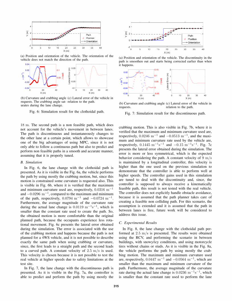
(a) Position and orientation of the vehicle. The orientation of thevehicle does not match the direction of the path.

0 20 40X (m)

-0.04

-0.02

0

0.02

0.04

κ (

m-1

)

0

0.05

0.1

β (

rad)

(b) Curvature and crabbing anglerequests. The crabbing angle sat-urates during the lane change.

0 10 20 30 40X (m)

-0.1

-0.05

0

0.05La

tera

l Err

or (

m)

(c) Lateral error of the vehicle inrelation to the path.

Fig. 6: Simulation result for the clothoidal path.

18 m. The second path is a non feasible path, which doesnot account for the vehicle’s movement in between lanes.The path is discontinuous and instantaneously changes tothe other lane at a certain point, which allows to showcaseone of the big advantages of using MPC, since it is notonly able to follow a continuous path but also to predict andperform non feasible paths in a smooth and accurate manner,assuming that it is properly tuned.

B. SimulationIn Fig. 6, the lane change with the clothoidal path is

presented. As it is visible in the Fig. 6a, the vehicle performsthe path by using mostly the crabbing motion, but, since thismotion is constrained some curvature is requested also. Thisis visible in Fig. 6b, where it is verified that the maximumand minimum curvature used are, respectively, 0.0316 m−1

and −0.0296 m−1, compared to the maximum and minimumof the path, respectively, 0.0794 m−1 and −0.0724 m−1.Furthermore, the average magnitude of the curvature rateduring the actual lane change is 0.0119 m−1s−1, which issmaller than the constant rate used to create the path. So,the obtained motion is more comfortable than the originalplanned path, because the occupants experience less rota-tional movement. Fig. 6c presents the lateral error obtainedduring the simulation. The error is associated with the useof the crabbing motion and happens because the path is notplanned for a 4WS vehicle, and it is not possible to describeexactly the same path when using crabbing or curvature,since, the first leads to a straight path and the second leadsto a curved path. A constant velocity of 2.5 m/s is used.This velocity is chosen because it is not possible to test thereal vehicle at higher speeds due to safety limitations at thetest site.

In Fig. 7, the lane change with the discontinuous path ispresented. As it is visible in the Fig. 7a, the controller isable to predict and perform the path by using mostly the

(a) Position and orientation of the vehicle. The discontinuity in thepath is smoothen out and starts being corrected earlier than whenit happens.

0 20 40X (m)

-0.06

-0.04

-0.02

0

0.02

κ (

m-1

)

-0.05

0

0.05

0.1

0.15

β (

rad)

(b) Curvature and crabbing anglerequests.

0 10 20 30 40X (m)

-1

0

1

2

Late

ral E

rror

(m

)

(c) Lateral error of the vehicle inrelation to the path.

Fig. 7: Simulation result for the discontinuous path.

crabbing motion. This is also visible in Fig. 7b, where it isverified that the maximum and minimum curvature used are,respectively, 0.0246 m−1 and −0.0513 m−1, and the maxi-mum and minimum curvature rate used by the vehicle are,respectively, 0.1445 m−1s−1 and −0.15 m−1s−1. Fig. 7cpresents the lateral error obtained during the simulation. Theerror is more or less symmetrical, which is the expectedbehavior considering the path. A constant velocity of 9 m/sis maintained by a longitudinal controller, this velocity ishigher than the one used on the previous simulation todemonstrate that the controller is able to perform well athigher speeds. The controller gains used in this simulationare tuned to deal with the discontinuity and, since, thecontroller is supposed to always receive a kinematicallyfeasible path, this result is not tested with the real vehicle.The controller does not explicitly handle obstacle avoidance,because it is assumed that the path planner takes care ofcreating a feasible non colliding path. For this scenario, theassumption is extended and it is assumed that the path inbetween lanes is free, future work will be considered toaddress this issue.

C. Experimental Results

In Fig. 8, the lane change with the clothoidal path per-formed at 2.5 m/s is presented. The results were obtainedusing the RCV, and performing the scenario in betweenbuildings, with snowy/icy conditions, and using motorcycletires without chains or studs. As it is visible in the Fig. 8a,the vehicle performs the path by using mostly the crab-bing motion. The maximum and minimum curvature usedare, respectively, 0.0447 m−1 and −0.0564 m−1, which aresmaller than the maximum and minimum curvature of thepath. Furthermore, the average magnitude of the curvaturerate during the actual lane change is 0.0236 m−1s−1, whichis smaller than the constant rate used to perform the lane

315

(a) Position and orientation of the vehicle. The oscillations beforeand after the lane change are mostly from GPS drift and were notnoticeable during the experiment.

0 20 40X (m)

-0.06

-0.04

-0.02

0

0.02

0.04

κ (

m-1

)

-0.1

-0.05

0

0.05

0.1

0.15

β (

rad)

(b) Curvature and crabbing anglerequests. The GPS drift leads tosome β and κ but the vehicleconverged always to the path.

0 10 20 30 40X (m)

-0.1

0

0.1

0.2La

tera

l Err

or (

m)

(c) Lateral error of the vehiclein relation to the path. Note, forexample, the jump in lateral errorthat occurred at 36.57 m, whichhappens because of the GPS.

Fig. 8: Experimental result for the clothoidal path.

change.The error presented in Fig. 8b, is not only associated with

the use of the crabbing motion as in the simulation, but alsowith GPS drift and the complex dynamics of the vehicle.The actuators installed on the RCV are worn and not veryprecise, which lead to bigger errors. Furthermore, a roughcalibration of the wheel alignment is done a priori, whichlead to unmodeled behavior. The GPS drift is bigger at thebeginning and at the end of the path, when the vehicle wascloser to buildings. This drift is clear around 36.57 m, wherewith the speed, orientation, and crabbing angle the vehiclehad, it is impossible for it to move 0.6 m sideways as theresults show.

VI. CONCLUSIONS AND FUTURE WORK

In this paper, an LTV-MPC for a 4WS vehicle is presented.The controller makes use of the additional degree of freedomof the vehicle to track a path in a smoother and comfortablemanner. To do this, not only the error to the path isminimized, but also the error to the road/desired direction.This way, the vehicle can crab, i.e., move sideways, to trackthe path, even when the desired orientation is not tangent tothe path.

The controller is able to predict and perform the pathusing not only curvature requests but also crabbing anglerequests, even for paths planned only assuming curvature.The vehicle was able to track a clothoidal lane change onicy/snowy conditions. It performed the lane change in asmooth and accurate manner, saturating the use of β, usinga maximum curvature magnitude of 0.0564 m−1 and anaverage curvature rate magnitude of 0.0236 m−1s−1, bothsmaller than the intended in the planned path.

The long term research goal of the RCV is to demonstratefully autonomous and connected mobility in city environ-ments. With respect to future controller development, thisbrings requirements for integrating with the larger scalesystem. For example, this may involve introducing stateconstraints provided by other functions in the system, inorder to guarantee collision free operation. This also impliesdoing further tests at different speeds, to guarantee robustnessand the generality of the solution proposed.

REFERENCES

[1] B. van Arem, C. J. G. van Driel, and R. Visser, “The impact ofcooperative adaptive cruise control on traffic-flow characteristics,”IEEE Transactions on Intelligent Transportation Systems, vol. 7, no. 4,pp. 429–436, December 2006.

[2] J. Ploeg, S. Shladover, H. Nijmeijer, and N. van de Wouw, “Intro-duction to the special issue on the 2011 grand cooperative drivingchallenge,” IEEE Transactions on Intelligent Transportation Systems,vol. 13, no. 3, pp. 989–993, September 2012.

[3] S. Thrun et al., “Stanley: The robot that won the darpa grandchallenge,” Journal of Field Robotics, vol. 23, no. 9, pp. 661–692,June 2006.

[4] C. Urmson et al., “Autonomous driving in urban environments:Boss and the urban challenge,” Journal of Field Robotics,vol. 25, no. 8, pp. 425–466, 2008. [Online]. Available:http://dx.doi.org/10.1002/rob.20255

[5] P. Falcone, F. Borrelli, J. Asgari, H. E. Tseng, and D. Hrovat,“Predictive active steering control for autonomous vehicle systems,”IEEE Transactions on Control Systems Technology, vol. 15, no. 3, pp.566–580, 5 2007.

[6] V. Turri, A. Carvalho, H. E. Tseng, K. H. Johansson, and F. Borrelli,“Linear model predictive control for lane keeping and obstacle avoid-ance on low curvature roads,” in Intelligent Transportation Systems -(ITSC), 2013 16th International IEEE Conference on, 10 2013, pp.378–383.

[7] T. Bak and H. Jakobsen, “Agricultural robotic platform withfour wheel steering for weed detection,” Biosystems Engineering,vol. 87, no. 2, pp. 125 – 136, 2004. [Online]. Available:http://www.sciencedirect.com/science/article/pii/S153751100300196X

[8] T. Bunte, L. M. Ho, C. Satzger, and J. Brembeck, “Central vehi-cle dynamics control of the robotic research platform robomobil,”ATZelektronik worldwide, 2014.

[9] Stanford volkswagen automotive innovation lab. [Online]. Available:http://web.stanford.edu/group/vail/

[10] Easymile mobility solution. [Online]. Available: http://easymile.com/[11] S. Sano, Y. Furukawa, and S. Shiraishi, “Four wheel steering system

with rear wheel steer angle controlled as a function of steering wheelangle,” SAE Technical Paper, Tech. Rep., 1986.

[12] Research concept vehicle. [Online]. Available:https://www.itrl.kth.se/research/itrl-labs/rcv-1.476469

[13] O. Wallmark et al., “Design and implementation of an experimentalresearch and concept demonstration vehicle,” in 2014 IEEE VehiclePower and Propulsion Conference (VPPC), Oct 2014, pp. 1–6.

[14] T. Keviczky, P. Falcone, F. Borrelli, J. Asgari, and D. Hrovat, “Pre-dictive control approach to autonomous vehicle steering,” in AmericanControl Conference, 2006, June 2006, pp. 6 pp.–.

[15] P. F. Lima, M. Trincavelli, M. Nilsson, J. Mrtensson, and B. Wahlberg,“Experimental evaluation of economic model predictive control for anautonomous truck,” in 2016 IEEE Intelligent Vehicles Symposium (IV),June 2016, pp. 710–715.

[16] J. Kong, M. Pfeiffer, G. Schildbach, and F. Borrelli, “Kinematic anddynamic vehicle models for autonomous driving control design,” in2015 IEEE Intelligent Vehicles Symposium (IV), June 2015, pp. 1094–1099.

[17] R. Rajamani, Vehicle Dynamics and Control.[18] J. Rossiter, Model-Based Predictive Control: A Practical Approach,

ser. Control Series. CRC Press, 2003. [Online]. Available:https://books.google.se/books?id=owznQTI-NqUC

[19] F. Kuhne, J. Gomes, and W. Fetter, “Mobile robot trajectory trackingusing model predictive control,” in II IEEE latin-american roboticssymposium, 2005.

[20] J. Mattingley and S. Boyd, “Cvxgen: A code generator for embeddedconvex optimization,” Optimization and Engineering, vol. 13, no. 1,pp. 1–27, 2012.

[21] Cvxgen. [Online]. Available: http://cvxgen.com/docs/index.html

316