Tutorials in Quantitative Methods for Psychology 2009, Vol. 5(1), p. 11‐24. 

                                                                 

Latent Class Growth Modelling: A Tutorial 

Heather Andruff, Natasha Carraro, Amanda Thompson, and Patrick Gaudreau University of Ottawa 

 Benoît Louvet 

Université de Rouen  

The  present  work  is  an  introduction  to  Latent  Class  Growth Modelling  (LCGM). LCGM is a semi‐parametric statistical technique used to analyze longitudinal data. It is used when  the data  follows a pattern of  change  in which both  the  strength and  the direction of the relationship between the independent and dependent variables differ across  cases.  The  analysis  identifies  distinct  subgroups  of  individuals  following  a distinct pattern of  change over age or  time on a variable of  interest. The aim of  the present  tutorial  is  to  introduce  readers  to LCGM and provide a concrete example of how the analysis can be performed using a real‐world data set and the SAS software package with accompanying PROC TRAJ application. The advantages and limitations of this technique are also discussed. 

  

 Longitudinal data  is  at  the  core of  research  exploring change  in  various  outcomes  across  a  wide  range  of disciplines. A number of statistical  techniques are available for analyzing  longitudinal data  (see Singer & Willet, 2003). 

    Heather  Andruff,  Natasha  Carraro,  Amanda  Thompson, and Patrick Gaudreau, School of Psychology, University of Ottawa; Benoît Louvet, Départment du Sport et l’Éducation Physique, Université de Rouen. Heather Andruff, Natasha Carraro, and Amanda Thompson played an equal role in the preparation of this manuscript and should all be considered as  first  authors.  This  research was  supported  by  a  Social Sciences  and  Humanities  Research  Council  Canada Graduate  Scholarship  awarded  to  Natasha  Carraro,  an Ontario  Graduate  Scholarship  awarded  to  Amanda Thompson,  and  a  regular  research  grant  from  the  Social Sciences  and  Humanities  Research  Council  and  the University  of  Ottawa  Research  Scholar  Fund  awarded  to Patrick Gaudreau.  

Correspondence concerning this article should be sent to Heather  Andruff,  University  of  Ottawa,  School  of Psychology,  145  Jean‐Jacques  Lussier  St., Ottawa, Ontario, Canada, K1N 6N5. Email: heather.andruff@uottawa.ca.  

One approach is to study raw change scores. By this method, change  is  computed  as  the difference  between  the  Time  1 and  the Time 2 scores and  the resulting raw change values are  analyzed  as  a  function  of  individual  or  group characteristics (Curran & Muthén, 1999). Raw change scores are  typically  analyzed  using  t‐tests,  analysis  of  variance (ANOVA), or multiple  regression. An alternative approach is to study residualized change scores. By this method, change is  computed  as  the  residual  between  the  observed Time  2 score  and  the  expected  Time  2  score  as  predicted  by  the Time 1 score (Curran & Muthén, 1999). Residualized change scores  are  typically  analyzed  using multiple  regression  or analysis of covariance (ANCOVA).  

Although both  raw  and  residualized  change  scores  can be  useful  for  analyzing  longitudinal  data  under  some circumstances,  one  limitation  is  that  they  tend  to  consider change between only  two discrete  time points and are  thus more  useful  for  prospective  research  designs  (Curran  & Muthén,  1999).  Frequently,  however,  researchers  are interested  in modelling developmental trajectories, or patterns of change  in an outcome across multiple  (i.e., at  least  three) time points (Nagin, 2005). For  instance, psychologists try to identify  the  course  of  various  psychopathologies  (e.g., Maughan,  2005),  criminologists  study  the  progression  of 

  11 

  12  criminality  over  life  stages  (e.g.,  Sampson  &  Laub,  2005), and  medical  researchers  test  the  impact  of  various treatments  on  the  progression  of  disease  (e.g.,  Llabre, Spitzer, Siegel, Saab, & Schneiderman, 2004).  

A  common  approach  to  studying  developmental trajectories is to use standard growth analyses such as repeated measures multivariate  analysis  of  variance  (MANOVA)  or structural  equation  modelling  (SEM;  Jung  &  Wickrama, 2008). Standard growth analyses estimate a single trajectory that averages the individual trajectories of all participants in a  given  sample.  Time  or  age  is  used  as  an  independent variable to delineate the strength and direction of an average pattern  of  change  (i.e.,  linear,  quadratic,  or  cubic)  across time  for  an  entire  sample. This  average  trajectory  contains an  averaged  intercept  (i.e.,  the  expected  value  of  the dependent  variable  when  the  value  of  the  independent variable(s) is/are equal to zero) and an averaged slope (i.e., a line representing the predicted strength and direction of the growth trend) for the entire sample. This approach captures individual  differences  by  estimating  a  random  coefficient that represents the variability surrounding this intercept and slope.  By  this method,  researchers  can  use  categorical  or continuous  independent  variables,  representing  potential risk or protective factors, to predict individual differences in the  intercept  and/or  slope  values.  By  centering  the  age  or time  variable,  a  researcher  may  set  the  intercept  to  any predetermined  value  of  interest.  For  instance,  a  researcher could use self‐esteem to predict individual differences in the intercept  of  depression  at  the  start,  middle,  or  end  of  a semester, depending on the research question. Results could indicate  that  people with  higher  self‐esteem  report  lower levels  of depression  at  the  start  of  the  semester.  Similarly, researchers  could  use  self‐esteem  to  predict  individual differences  in  the  linear  slope of depression. Results  could indicate  that  people  with  higher  self‐esteem  at  baseline experience  a  slower  increase  in depressive  symptoms over the  course  of  the  semester,  indicating  that  self‐esteem  is  a possible  protective  factor  against  a  more  severe  linear increase in depression.  

Standard growth models are useful for studying research questions  for which  all  individuals  in  a  given  sample  are expected  to  change  in  the  same direction  across  time with only  the  degree  of  change  varying  between  people (Raudenbush,  2001).  Nagin  (2002)  offers  time  spent  with peers  as  an  example  of  this  monotonic  heterogeneity  of change. With  few  exceptions,  children  tend  to  spend more time  with  their  peers  as  they  move  from  childhood  to adolescence.  In  this  case,  it  is  useful  to  frame  a  research question in terms of an average trajectory of time spent with peers.  However,  some  psychological  phenomena  may follow a multinomial pattern  in which both  the strength and 

the direction of change are varying between people (Nagin, 2002). Raudenbush (2001) uses depression as an example by arguing  that  it  is  incorrect  to  assume  that  all  people  in  a given  sample  would  be  experiencing  either  increasing  or decreasing  levels of depression.  In a normative  sample, he states, many people will never be high on depression, others will  always  be  high,  others  will  become  increasingly depressed,  while  others  may  fluctuate  between  high  and low levels of depression. In such instances, a single averaged growth  trajectory  could  mask  important  individual differences and lead to the erroneous conclusion that people are  not  changing  on  a  given  variable.  Such  conclusions could be drawn if 50% of the sample increased by the same amount on a particular variable whereas 50% of the sample decreased  by  the  same  amount  on  that  variable.  Here,  a single  growth  trajectory  would  average  to  zero,  thus prompting  researchers  to  conclude  an  absence  of  change despite the presence of substantial yet opposing patterns of change  for  two distinct  subgroups  in  the  sample  (Roberts, Walton,  &  Viechtbauer,  2006).  For  this  class  of  problems, alternative modelling  strategies  are  available  that  consider multinomial heterogeneity in change. One such approach is a  group‐based  statistical  technique  known  as  Latent Class Growth Modelling (LCGM). 

Theoretical basis of LCGM 

Given the substantial contribution of Nagin (1999; 2005) to both the theory and methodology of LCGM, the following explanations of the technique draw primarily from his work and  from  recent  extensions  proposed  by  his  collaborators. LCGM  is  a  semi‐parametric  technique  used  to  identify distinct subgroups of individuals following a similar pattern of  change  over  time  on  a  given  variable.  Although  each individual  has  a  unique  developmental  course,  the heterogeneity or the distribution of individual differences in change  within  the  data  is  summarized  by  a  finite  set  of unique  polynomial  functions  each  corresponding  to  a discrete  trajectory  (Nagin, 2005). Given  that  the magnitude and direction of change can vary freely across trajectories, a set  of  model  parameters  (i.e.,  intercept  and  slope)  is estimated  for  each  trajectory  (e.g.,  Nagin,  2005).  Unlike standard  latent  growth  modelling  techniques  in  which individual  differences  in  both  the  slope  and  intercept  are estimated using  random coefficients, LCGM  fixes  the slope and  the  intercept  to  equality  across  individuals  within  a trajectory.  Such  an  approach  is  acceptable  given  that individual  differences  are  captured  by  the  multiple trajectories included in the model. Given that both the slope and  intercept  are  fixed,  a  degree  of  freedom  remains available  to  estimate  quadratic  trajectories  of  a  variable measured at three time points or cubic trajectories with data 

 

  13  

)*it

available at four time points.  Although the model is widely applicable, the rating scale 

of  the  instrument used  to measure  the  variable  of  interest dictates the specific probability distribution used to estimate the parameters. Psychometric scale data necessitate  the use of  the  censored  normal  model  distribution,  dichotomous data  require  the  use  of  the  binary  logit  distribution,  and frequency  data  dictate  the  use  of  the  Poisson  distribution. For example,  in the censored normal model, each trajectory is  described  as  a  latent  variable (y   that  represents  the predicted  score  on  a  given  dependent  variable  of  interest 

  for  a  given  trajectory ( )Υ ( )j at  a  specific  time  ( )t and  is defined by the following function:  

  ( ) 0 1 3j j j

it it ity* 22j

it3

itβ β βΧ + β= + Χ + ε

it

Χ +   

In this equation, , , and   represent the independent variable (i.e., Time or Age) entered in a regular, squared, or cubed  term, respectively. Further, 

itΧ 2itΧ 3

itΧ

ε   is a disturbance  term assumed to be normally distributed with a mean of zero and a  constant  standard  deviation.  Finally, 0

jβ ,  1jβ ,  2

jβ ,  and 

3jβ are the parameters defining the intercept and slopes (i.e., 

linear,  quadratic,  cubic)  of  the  trajectory  for  a  specific subgroup  ( )j .  As  demonstrated  in  the  above  polynomial function,  the  trajectories  are  most  often  modelled  using either a  linear  ( )itΧ , quadratic  , or cubic ( )2

itΧ ( )3itΧ   trend, 

depending on the number of time points measured. A linear pattern of  change  is defined by  the  ( )itΧ

(Χ

)3itΧ

 parameter and a linear  trend  may  either  steadily  increase  or  decrease  at varying magnitudes or remain stable. A quadratic pattern of change  is defined by  the   parameter  and  a quadratic trend  may  increase,  decrease,  or  remain  stable  up  to  a certain  time  point  before  changing  in  either magnitude  or direction.  Furthermore,  a  cubic  trajectory  is  defined  by the ( parameter and a cubic trend will have two changes in either the magnitude or direction across time points.  

)2it

Using  LCGM,  researchers must  specify  the  number  of distinct  trajectories  to be extracted  from  the data and select the model with  the number of  trajectories  that best  fits  the data. It is preferable to have a priori knowledge concerning the number  and  the  shape  of  trajectories whenever  theory and  literature  exists  in  the  area  of  study.  Researchers evaluate which model provides  the  best  fit  to  the data  by interpreting  and  comparing  both  the  fit  statistics  and  the posterior  probabilities  for  each model  tested.  The  Bayesian Information Criterion  (BIC) value  is obtained  for each model tested and is a fit index used to compare competing models that  include different numbers of  trajectories or  trajectories of  various  shapes  (e.g.,  linear  versus  quadratic).  More specifically,  nested  models  testing  the  inclusion  of  a different number of  trajectories  can be  compared using  an estimate  of  the  log  Bayes  Factor  defined  by  the  following 

formula (Jones, Nagin, & Roeder, 2001):  

( ) ( )102 log 2 BICe Β ≈

The  estimate  is  approximately  equal  to  two  times  the difference  in  the  BIC  values  for  the  two  models  being compared. Here,  the difference  is calculated by  subtracting the BIC value of the simpler model (i.e., the model with the smaller  number  of  trajectories)  from  the  more  complex model  (i.e.,  the  model  with  the  larger  number  of trajectories).  A  set  of  guidelines  has  been  adopted  for interpreting the estimate of the log Bayes Factor in order to measure  the  extent  of  evidence  surrounding  the  more complex  model  thereby  ensuring  model  parsimony. According to these guidelines, values ranging from 0 to 2 are interpreted as weak evidence  for  the more complex model, values  ranging  from  2  to  6  are  interpreted  as  moderate evidence,  values  ranging  from  6  to  10  are  interpreted  as strong evidence, and values greater  than 10 are  interpreted as very strong evidence (Jones et al., 2001). Initially, for each model,  the  linear,  quadratic,  and  cubic  functions  of  each trajectory  can be  tested, depending on  the number of  time points.  To  ensure  parsimony,  consistent  with  the recommendations of Helgeson, Snyder, and Seltman (2004), non‐significant cubic and quadratic terms are removed from trajectories  in  a  given  model,  but  linear  parameters  are retained  irrespective  of  significance  (as  cited  in  Louvet, Gaudreau, Menaut,  Genty,  &  Deneuve,  2009).  Once  non‐significant terms have been removed, each model is retested yielding  a new BIC value. The  fit of  each nested model  is then  compared  using  the  estimate  of  the  log Bayes  factor. This process of comparing  the  fit of each subsequent, more complex model,  to  the  fit of  the previously  tested,  simpler model,  continues until  there  is no  substantial  evidence  for improvement  in model  fit.  In  addition,  both  the  posterior probabilities  and  the  averaged  group  membership probabilities for each trajectory are examined to evaluate the tenability of each model. 

The parameter  coefficients  estimated  in LCGM provide direct  information  regarding  group  membership  prob‐abilities. A group membership probability  is  calculated  for each trajectory and corresponds to the aggregate size of each trajectory or the number of participants belonging to a given trajectory.  Ideally,  each  trajectory  should  hold  an approximate group membership probability of at  least  five percent. However, in clinical samples, some trajectories may model the profile of change of only a fraction of the sample. Posterior  probabilities  can  be  calculated  post  hoc  to 

estimate  the  probability  that  each  case, with  its  associated profile of change,  is a member of each modelled  trajectory. The  obtained  posterior  probabilities  can  be  used  to  assign each  individual  membership  to  the  trajectory  that  best 

 

  14  

 Figure 1.  Syntax window with the associated data set. 

 

terior  probabilities  o

erior probabilities of p

matches his or her profile of change. A maximum‐probability assignment  rule  is  then  used  to  assign  each  individual membership  to  the  trajectory  to which he or  she holds  the highest  posterior  membership  probability.  An  example demonstrating  the  use  of  the  maximum  probability assignment  rule  is  presented  below.  Table  1  displays  a hypothetical  data  set  with  six  individuals  whose developmental  course on  a variable  are modelled by  three trajectories,  thus  resulting  in  three  posterior  probability values for each  individual. Using the maximum probability assignment  rule,  participants  1  and  5  would  be  assigned group  membership  to  Trajectory  3,  participants  2  and  3 would  be  considered  as  members  of  Trajectory  2,  and participants 4 and 6 would be regrouped into Trajectory 1.  

The  average  posterior  probability  of  group  membership  is calculated  for  each  trajectory  identified  in  the  data.  The average  posterior  probability  of  group membership  for  a trajectory  is an approximation of  the  internal  reliability  for 

each  trajectory.  This  can  be  calculated  by  averaging  the posterior probabilities of  individuals having been assigned group  membership  to  a  trajectory  using  the  maximum probability assignment rule. Average posterior probabilities of  group membership  greater  than  .70  to  .80  are  taken  to indicate  that  the  modelled  trajectories  group  individuals with  similar patterns of  change and discriminate between individuals with dissimilar patterns of change. Returning to the hypothetical data set displayed in Table 1, the posterior probabilities  of  participants  4  and  6 with  Trajectory  1  are averaged  to  obtain  the  average  pos f group membership  for Trajectory 1  [ ( )0.93 1.00 2 0.97+ ÷ = ] as are the post articipants 2 and 3 with Trajectory  2  [ ( )1.00 .86 2 0.93+ ÷ = ],  and  the  posterior p[robabilities  of  participants  1  and  5  with  Trajectory  3 ( )1.00 .76 2 0.88+ ÷ = ].  

Table 1. Hypothetical data set with six participants and three trajectories

  Posterior Probability Participants  Trajectory 1  Trajectory 2  Trajectory 3 

1  .10  .10  .80 2  .00  1.00  .00 3  .04  .86  .10 4  .93  .02  .05 5  .20  .03  .76 6  1.00  .00  .00 

 

  15  

 in 

ebsite: htt

 

Knight,  Sidani,  &  Figueredo,  2007).  Given this,  it  is  recommended  that  any missing  data  be  treated 

Performing LCGM using SAS 

For  illustration  purposes,  a  data  set  obtained  with permission  from  Louvet,  Gaudreau,  Menaut,  Genty,  and Deneuve (2007) will be used to demonstrate how to perform the LCGM analyses (see Appendix A). This data set, labelled DISEN,  includes  a  measure  of  disengagement  coping  at three time points for 107 participants. Typically, a data set of at  least  300  to  500  cases  is  preferable  for  running  LCGM, although  the analysis can be applied  to data sets of at  least 100 cases (Nagin, 2005). It should be noted that performing LCGM with  smaller  sample  sizes  limits  the  power  of  the analysis  as well  as  the  number  of  identifiable  trajectories (Nagin, 2005). In such instances, as in the example presented

this  tutorial,  the  researcher  may  adopt  a  more  liberal significance criterion (e.g., p < .10; Tabachnick & Fidell, 2007) which is then applied consistently throughout the analysis.  

In order to perform the analysis using SAS, the user has to  install  the  PROC  TRAJ  application  (Jones  et  al.,  2001) which  is  freely  available  at  the  following  w

p://www.andrew.cmu.edu/user/bjones/.  Complete  ins‐tructions  for  downloading  and  installing  the  PROC  TRAJ application are available on the website (Jones, 2005). 

Before  running  the  analysis  using  the  PROC  TRAJ application  in SAS, the data set to be analyzed will need to be  imported  from  the  computer program  on which  it was prepared (e.g., Excel). The variables from the data set should be  labelled  before  being  imported  into  SAS.  As  seen  in Figure 1, the first column in our data set is labelled “ID” and 

identifies each case in the data set. Each row should contain the data of one individual, or case. The next columns are the dependent variable  scores.  In  this data  set,  there  are  three measures of disengagement coping, one at each  time point. Thus, in this example, the second column is disengagement coping at Time 1, the third column is disengagement coping at Time 2, and the fourth column is disengagement coping at Time  3.  The  next  columns  in  the  data  set  are  variables representing  the  time  points  at  which  the  dependent variable was measured; in this example, columns 5, 6, and 7 represent Time 1, Time 2, and Time 3,  respectively.  In  this data set, each measurement point  is separated by  the same amount of time; therefore, Time 1 is coded as “0”, Time 2 is coded as “1”, and Time 3 is coded as “2”. However, LCGM can  be  performed  even when  the measurement  points  are separated by different time intervals that are relevant to the data  analysis  (e.g.,  Time  1  =  baseline,  Time  2  =  1 month, Time 3 = 6 months). In these instances, the user can code the time  variable  to  represent  the  age  or  time  of  each measurement  point  (e.g.,  5,  7,  13  [years  old]  or  1,  6,  18 [months since baseline]). The specific age/time can also vary across  individuals  to  account  for  the  fact  that  it  is  often impossible to measure each case at the exact same time. For this reason, the time variable is entered individually for each case  in  the database. Also,  it  is  important  to note  that SAS uses an  imputation procedure  to assign values  for missing data  which  may  not  be  suitable  for  every  data  set (McKnight,  Mc

 Figure 2.  Syntax for the analysis of a model with one quadratic trajectory. 

 

  16  

 

will open where  the  location f  the  data  on  the  computer  is  entered.  Second,  the  user 

c  the following three liautomatically as it is entered): 

the data set can be 

ts,  the  first  model  tests  the uadratic  parameters  for  one  trajectory  (defined  in  the 

smp 

ed  value  of  the  dependent  variable  at  each me

if y. Fi

point.  To run the a

w wll  o

ow. 

r  s d

prior  to  importing  the  data  set  into  the  PROC  TRAJ application.  

To  import  the  data  into  SAS,  four  steps  must  be followed.  First,  the  user  selects  Import  Data  from  the  File drop‐down menu. A window olicks on the syntax window and entersnes of syntax (please note, the colour of the text will change  in  any wa

 

 Third, once the syntax has been entered, copied  and  pasted  into  the  syntax  window  from  a 

program  like Excel. Finally, on  the next  line  after  the data set,  the  syntax  “RUN;”  is  entered.  Figure  1  provides  an example of the syntax window at this point. 

After adding the data set to the syntax window, the user enters the syntax to run the analysis. In this case, given that there  are  three  time  poinqyntax  as NGROUPS  1)  using  the  following  syntax.  For  a ore  complete  description  of  each  of  the  syntax  items, lease refer to Appendix B. 

 

The syntax “PROC PRINT DATA=OP” provides a  table of  the  predict

asurement  point  for  each  trajectory.  These  values  are used to create a figure depicting the shape of each trajectory. SAS provides a figure with low resolution that may need to be recreated using an alternative statistical program such as 

hs are to be used in publication or modified gure  2  illustrates  the  syntax window  at  this 

nalysis, the user clicks the icon of the person running  in  the  top  right hand corner of  the syntax windo .  The  analysis  ill  run  and the  graph  of  the  trajectory  wi pen  in  a new wind To view  the actual output of 

the analysis, the user clicks on the Output window located in the bar at the bottom of the screen. The output for this one quadratic  trajectory model  is displayed  in Figure 3.  In each output, statistics are provided fo each e timate  parameter including  the  intercept

SPSS  the grap

( )0β ,  the  linear parameter ( )1β , and the  quadratic  param )2eter  (β for  each  trajectory.  The intercept  ( )0β corresponds  to  the  value  of  the  dependent variable when the value of the independent variable is equal to  zero.  A  t‐test  for  the  intercept  provi   in  the  output 

e  value  of  the  dependent  variable from  zero  when  the  independent ro. The linear slope parameter estimate 

dedhether  th  differs 

ble is equal to ze

indicates  wsignificantlyvaria( )1β   represents  the  amount  of  increase/decrease  on  the 

dependent  variable  for  each  unit  of increase  on  the  independent  variable (e.g., Time 1 to Time 2). The quadratic slope  parameter  estimate  ( )2β  represen s  th   mount  of increase/decrease  on  the  dependent variable  for  each  unit  of  increase  on the squared independent variable. The amount  of  variance  in  the  data accounted  for  by  the  model  and  its 

significance  is  given  by  Sigma.  The  above  information  is 

 ic trajectory. Figure 3.  Output from the analysis of a model with one quadrat

DR

ATA <NAME OF DATABASE>; INPUT ID <DEPENDENT VARIABLES> <INDEPENDENT VACARDS;

IABLES>;

PROC TRAJ DATA=<DATABASE> OUT=OF OUTPLOT=OP OUTSTAT=OS T=OE ITDETAIL ALTSTART;

ID; VAR <DEPENDENT VARIABLES>; INDEP <INDEPENDENT

CNORM; MAX <MAX SCORE OF DEP. VAR.>; NGROUPS 1; ORDER 2;

RUN ; PR

OUTESIDVARIABLES>; MODEL t e a

OC PRINT DATA=OP; RUN ;  

  17  

 the second BIC value is interpreted as the index of 

model  for one  linear  trajectory  is  run  to determine  the BIC 

t significant, the

r B

i

r of the qua

can be run (syntax “ORDER 1 2” or “ORDER 2 1”).    e     

 the second BIC value is interpreted as the index of 

model  for one  linear  trajectory  is  run  to determine  the BIC 

t significant, the

r B

i

r of the qua

can be run (syntax “ORDER 1 2” or “ORDER 2 1”).    e     

read  from  the  Output  for  each model.  The  Group  column labels  the  number  of  trajectories  tested  and  the  Parameter column  labels  the  estimated  parameters.  The  test  statistic, standard  error,  and  significance  for  each  parameter  are displayed  in  the Estimate column,  the Standard Error column, the Prob > |T| column, respectively. The T for H0: Parameter = 0 column provides a value for the test of the null hypothesis that determines whether the parameter is significant or not. The value of the t‐test has to be higher than 1.96 (p < .05) or 2.58  (p  <  .01).  Two  BIC  values  are  also  provided  in  each output and

 hypothesis that determines whether the parameter is significant or not. The value of the t‐test has to be higher than 1.96 (p < .05) or 2.58  (p  <  .01).  Two  BIC  values  are  also  provided  in  each output and

fit  for  the  model.  In  this  analysis  modelled  with  one quadratic  trajectory,  the  results  can  be  summarized  as follows: β0 = 2.09, p = .000; β1=.028, p = 0.86; and β2 = .01, p = .92; Sigma =  .62, p =  .000; BIC =  ‐309.79  (see Figure 3). The user  can  also  scroll  down  in  this  window  to  view  the predicted  values  of  the  dependent  variable  at  different values  of  the  independent  variable  for  each  point  on  the graph.  

As a general rule, for data sets with three time points, a single  quadratic  trajectory  model  is  tested  first.  If  the quadratic  component  of  this model  is  not  significant,  the 

fit  for  the  model.  In  this  analysis  modelled  with  one quadratic  trajectory,  the  results  can  be  summarized  as follows: β0 = 2.09, p = .000; β1=.028, p = 0.86; and β2 = .01, p = .92; Sigma =  .62, p =  .000; BIC =  ‐309.79  (see Figure 3). The user  can  also  scroll  down  in  this  window  to  view  the predicted  values  of  the  dependent  variable  at  different values  of  the  independent  variable  for  each  point  on  the graph.  

As a general rule, for data sets with three time points, a single  quadratic  trajectory  model  is  tested  first.  If  the quadratic  component  of  this model  is  not  significant,  the 

best  fit  is  obtained,  as  determined  by  comparing  the  BIC values. 

Coming  back  to  our  example,  since  the  quadratic component of  the one  trajectory model was no

best  fit  is  obtained,  as  determined  by  comparing  the  BIC values. 

Coming  back  to  our  example,  since  the  quadratic component of  the one  trajectory model was no model  for  one  linear  trajectory  is  run  by  changing  the 

order of the model from 2 (for quadratic) to 1 (for linear) in the syntax window. The rest of the syntax remains the same. After running  this analysis, a new graph and a new output with the  equired  IC value is also generated.  

To  run  the  analysis  for  the  quadratic  model  for  two trajectories the user changes the syntax from “NGROUPS 1” to “NGROUPS 2” to estimate two trajectories. The syntax for the order  is also changed to “ORDER 2 2”. When using the ORDER  syntax,  the  f rst  number  represents  the  first trajectory  and  the  second  number  represents  the  second trajectory. Further,  a  “2”  indicates  the  trajectory  should be modelled  on  a  quadratic  trend whereas  a  “1”  indicates  a linear trend. This analysis can now be run.  If neithe

 model  for  one  linear  trajectory  is  run  by  changing  the order of the model from 2 (for quadratic) to 1 (for linear) in the syntax window. The rest of the syntax remains the same. After running  this analysis, a new graph and a new output with the  equired  IC value is also generated.  

To  run  the  analysis  for  the  quadratic  model  for  two trajectories the user changes the syntax from “NGROUPS 1” to “NGROUPS 2” to estimate two trajectories. The syntax for the order  is also changed to “ORDER 2 2”. When using the ORDER  syntax,  the  f rst  number  represents  the  first trajectory  and  the  second  number  represents  the  second trajectory. Further,  a  “2”  indicates  the  trajectory  should be modelled  on  a  quadratic  trend whereas  a  “1”  indicates  a linear trend. This analysis can now be run.  If neithe

dratic  components  of  the  two‐trajectory  model  is significant,  the  linear model can be  run  (syntax “ORDER 1 1”). Likewise, if only one component is significant, a model with  one  quadratic  component  and  one  linear  component 

dratic  components  of  the  two‐trajectory  model  is significant,  the  linear model can be  run  (syntax “ORDER 1 1”). Likewise, if only one component is significant, a model with  one  quadratic  component  and  one  linear  component 

value  for  this  model.  If  the  quadratic  component  of  the model  for  one  trajectory  is  significant,  the  analysis  for  the quadratic model for two trajectories is performed. Following these  analyses,  the  BIC  value  of  the  appropriate  two‐trajectory model will be  compared  to  the BIC value of  the appropriate  one‐trajectory model.  This  process  is  repeated with an increasing number of trajectories until the model of 

In our example, given that both quadratic components ofthe  two‐trajectory  model  are  significant,  the  BIC  valueobtained  from  this  analysis  is  compared  to  the  BIC  valufrom  the  previous  analysis  to  test  for  improvement  of  fit.Using  this  data  set  as  an  example,  the  model  with  twoquadratic  trajectories  (BIC  =  ‐289.05)  is  compared  to  themodel with  one  linear  trajectory  (BIC  =  ‐307.79)  using  the

value  for  this  model.  If  the  quadratic  component  of  the model  for  one  trajectory  is  significant,  the  analysis  for  the quadratic model for two trajectories is performed. Following these  analyses,  the  BIC  value  of  the  appropriate  two‐trajectory model will be  compared  to  the BIC value of  the appropriate  one‐trajectory model.  This  process  is  repeated with an increasing number of trajectories until the model of 

In our example, given that both quadratic components ofthe  two‐trajectory  model  are  significant,  the  BIC  valueobtained  from  this  analysis  is  compared  to  the  BIC  valufrom  the  previous  analysis  to  test  for  improvement  of  fit.Using  this  data  set  as  an  example,  the  model  with  twoquadratic  trajectories  (BIC  =  ‐289.05)  is  compared  to  themodel with  one  linear  trajectory  (BIC  =  ‐307.79)  using  the

 Figure 4.  Output from the analysis of a model with three quadratic trajectories. 

 

  18  

  of  the  log  Bayes  factor.  The  estimate  of  the  log ayes factor is calculated as follows:  

 Figure 5. Output from the analysis of a quadratic model for Trajectories  1 and 3 and linear model for Trajectory 2. 

estimateB

( ) ( )2 289.05 307.79 37.48⎡ ⎤× − − − =⎣ ⎦

Using the guidelines for  interpreting the estimate of the log  Bayes  factor  (Jones  et  al.,  2001),  these  results  provide very  strong  evidence  for  the  model  with  two  quadratic trajectories  compared  to  a  model  with  one  trajectory. However,  it  is necessary  to  continue  testing more  complex models with an increasing number of trajectories in order to det

n o   t 2

criterion  (p  =  0.10;  Tabachnick & Fo‐trajectory  model 

ermine  if  the model with  two  trajectories  provides  the best fit to the data.  

Next, a model with three quadratic trajectories is run by changing the syntax from “NGROUPS 2” to “NGROUPS 3” and  by  changing  the  order  to  read  “ORDER  2  2  2”.  The output of  this model, displayed  in Figure 4, shows  that  the quadratic  terms  of  Trajectory  1  and  Trajectory  3  are significant whereas  the quadratic parameter of Trajectory 2 is not significant. Given this, the user can test a model with two quadratic trajectories and one linear trajectory with the following sy tax c des indicating that Trajec ory   is linear: “NGROUPS  3; ORDER  2  1  2”. As  shown  in  Figure  5,  the results  of  this  analysis  indicate  that  all  modelled components of the trajectories can be considered significant as the small sample size warrants a more liberal significance 

  idell,  2007). Comparing this  three‐trajectory  model  to  the  tw

( ) ( )2× −

continues  until  there  is  no 

ries. Comparing  this model with

282.06 289.05 13.98⎡ ⎤− − =⎣ ⎦   provides  very  strong evidence for the three‐trajectory model.  

significant  improvement  in  model  fit  compared  to  the previously  tested model.  For  this  example,  an  analysis  for four  quadratic  trajectories  is  run,  followed  by  a  model deleting  the non‐significant components of each of  the  four trajecto   the  three‐trajectory model 

The  addition  of  trajectories 

( ) ( )2 285.89 282.06⎡ ⎤× − − − = −⎣ ⎦ 7.66   reveals  a decrease in f

ng (β0 = 3.16, p < 0.001; β1 = 1.47, p = 0.02; β2 = ‐0.70, p = 0.02).  

it for the four‐trajectory model.  As a result, the  three‐trajectory model  is retained as  the 

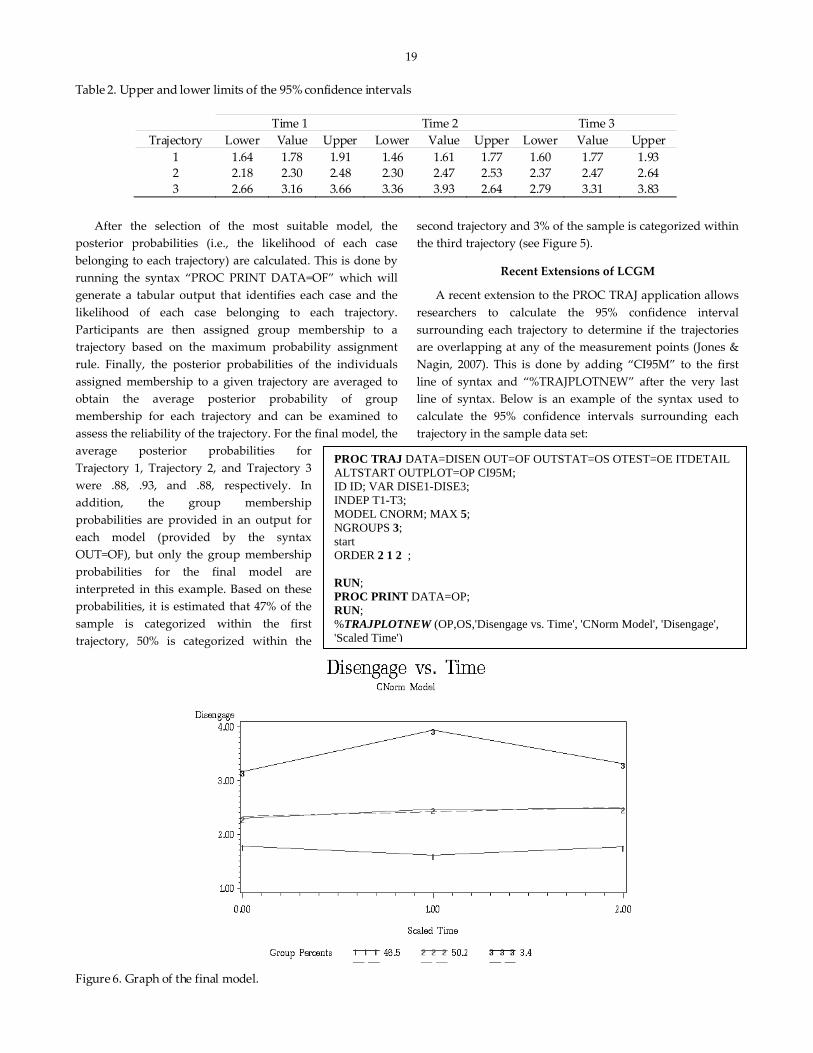
final and most parsimonious model. The output for this final model is displayed in Figure 5 and the parameters presented in the output will be interpreted. Figure 6 displays the graph for this final model with Trajectory 1 shown on the bottom, Trajectory 2  in  the middle, and Trajectory 3 on  top. Trajec‐tory  1  follows  a  quadratic  trend  in which  disengagement coping decreases  from Time 1  to Time 2 and  returns  to  its initial  level  by  Time  3.  The  participants whose  profiles  of change are best represented by Trajectory 1 tended to report low  levels of disengagement  coping which decreased  from Time  1  to Time  2  and  then  returned  to  the  initial  level by Time 3 (β0 = 1.78, p < 0.001; β1 = ‐.032, p = 0.07; β2 = 0.16, p = 0.06). Trajectory 2, which  follows a  linear  trend,  represents the  profile  of  change  of  the  participants  who  reported moderate  levels of disengagement at Time 1  followed by a marginally significant linear increase across time (β0 = 2.33, p < 0.001; β1 = 0.09, p = 0.07). Trajectory 3  follows a quadratic trend in which disengagement coping increases from Time 1 to Time  2  and  then decreases  by Time  3. The participants whose profiles of change are best represented by Trajectory 3 tended to report high levels of disengagement copi

 

  19  Table 2. Upper and lower limits of the 95% confidence intervals 

  Time 1  Time 2  Time 3 Trajectory  Lower  Value  Upper  Lower  Value  Upper  Lower  Value  Upper 

1  1.64  1.78  1.91  1.46  1.61  1.77  1.60  1.77  1.93 2  2.18  2.30  2.48  2.30  2.47  2.53  2.37  2.47  2.64 3  2.66  3.16  3.66  3.36  3.93  2.64  2.79  3.31  3.83 

 After  the  selection  of  the  most  suitable  model,  the 

posterior  probabilities  (i.e.,  the  likelihood  of  each  case belonging to each trajectory) are calculated. This is done by running  the  syntax  “PROC PRINT DATA=OF” which will generate  a  tabular output  that  identifies  each  case  and  the likelihood  of  each  case  belonging  to  each  trajectory. Participants  are  then  assigned  group  membership  to  a trajectory  based  on  the  maximum  probability  assignment rule.  Finally,  the  posterior  probabilities  of  the  individuals assigned membership  to a given  trajectory are averaged  to obtain  the  average  posterior  probability  of  group membership  for  each  trajectory  and  can  be  examined  to assess the reliability of the trajectory. For the final model, the average  posterior  probabilities  for Trajectory  1, Trajectory  2,  and Trajectory  3 were  .88,  .93,  and  .88,  respectively.  In addition,  the  group  membership probabilities  are provided  in  an output  for each  model  (provided  by  the  syntax OUT=OF), but only  the group membership probabilities  for  the  final  model  are interpreted  in  this example. Based on  these probabilities,  it  is estimated that 47% of the sample  is  categorized  within  the  first trajectory,  50%  is  categorized  within  the 

second trajectory and 3% of the sample is categorized within the third trajectory (see Figure 5). 

Recent Extensions of LCGM  

A recent extension to the PROC TRAJ application allows researchers  to  calculate  the  95%  confidence  interval surrounding  each  trajectory  to determine  if  the  trajectories are overlapping at any of the measurement points (Jones & Nagin,  2007). This  is done  by  adding  “CI95M”  to  the  first line  of  syntax  and  “%TRAJPLOTNEW”  after  the  very  last line  of  syntax. Below  is  an  example  of  the  syntax  used  to calculate  the  95%  confidence  intervals  surrounding  each trajectory in the sample data set:  

PROC TRAJ DATA=DISEN OUT=OF OUTSTAT=OS OTEST=OE ITDETAIL ALTSTART OUTPLOT=OP CI95M; ID ID; VAR DISE1-DISE3; INDEP T1-T3; MODEL CNORM; MAX 5; NGROUPS 3; start ORDER 2 1 2 ; RUN; PROC PRINT DATA=OP; RUN; %TRAJPLOTNEW (OP,OS,'Disengage vs. Time', 'CNorm Model', 'Disengage', 'Scaled Time')

 Figure 6. Graph of the final model.   

  20  

This  syntax  yields  a  new  graph  of  the  trajectories  that includes  the upper  and  lower  confidence  interval  for  each trajectory.  It  also  provides  an  output  with  the  numerical values of the confidence intervals for each trajectory at each time  point,  as  shown  in  Table  2.  For  a  more  detailed description  of  this  extension  and  several  others,  including performing LCGM with covariates, please refer to Jones and Nagin  (2007)  and  Gaudreau,  Amiot,  and  Vallerand  (in press). 

Another extension allows researchers to test whether the intercept and the slopes are significantly different across the trajectories  using  equality  constraints,  also  known  as invariance  testing  (Jones & Nagin,  2007). The Wald  test  is the  statistical  test  used  to  compare  the  intercepts  ( )0β as well  as  the  linear  ( )1β   and  quadratic  ( )2β   growth  com‐ponents  of  the  trajectories  to  determine whether  they  are significantly different  across  trajectories. Using  the  sample data  set,  it  is  possible  to  compare  if  there  is  a  significant difference between the intercepts of any two trajectories. As an example, to compare the intercepts of Trajectories 1 and 3 the  following  syntax  is  added  to  the  line  following  the ORDER command:  

 This  analysis  revealed  that  the  intercepts  of  these  two 

trajectories were  significantly  different  (  χ2  (1)  =27.68,  p  < .0001),  thus  indicating  that  Trajectory  3  had  a  greater disengagement  score  at  the  time  point  on  which  the independent variable was  centered  (i.e., Time 1 was  coded as 0;  see Figure 1)  .To  compare  the  slopes of Trajectories 1 and 3, the “%TRAJTEST” syntax is changed to read:   %TRAJTEST(ʹlinear1=linear3,quadra3=quadra1ʹ) /*linear&quadratic equality test*/  

The rest of the syntax remains the same and this analysis reveals that the slopes of these two quadratic trajectories are also  significantly  different,  χ2  (2)  =7.64  p  <  .05,  which 

indicates  that  the quadratic  slope of Trajectory 3  is  steeper than that of Trajectory 1.  

Conclusion  

LCGM  is  a  useful  technique  for  analyzing  outcome variables  that  change  over  age  or  time.  This  method provides  a  number  of  advantages  over  standard  growth modelling  procedures.  First,  rather  than  assuming  the existence  of  a  particular  type  or  number  of  trajectories  a priori, this method uses a formal statistical procedure to test whether the hypothesized trajectories actually emerge from the  data  (Nagin,  2005).  As  such,  the method  permits  the discovery  of  unexpected  yet  potentially  meaningful trajectories  that  may  have  otherwise  been  overlooked (Nagin,  2005).  LCGM  also  bypasses  a  host  of  other challenges  (e.g., over‐ or under‐fitting  the data,  trajectories reflecting  only  random  variation)  associated  with assignment  rules  sometimes  used  in  conjunction  with standard  growth  modelling  approaches  (Nagin,  2002). Although  not  presented  in  detail  here,  extensions  of  the basic LCGM model also allow the researcher to estimate the probability  that  an  individual  will  belong  to  a  particular 

trajectory  based  on  their  score  on  a covariate.  Other  extensions  allow  the researcher  to  obtain  estimates  of whether a turning point event (such as an  intervention  or  important  life transition)  can  alter  a  developmental trajectory  (see  Nagin,  2005;  Jones  & Nagin,  2007).  In  addition,  LCGM serves  as  a  steppingstone  to  growth mixture modelling  analyses  in which the precise number and shape of each trajectory must  be  known  a  priori  in order  for  the  researcher  to  impute  the requisite  start values  for  the model  to converge in software packages such as 

Mplus  (Jung & Wickrama, 2008). Finally,  the method  lends itself  well  to  the  presentation  of  results  in  graphical  and tabular format, which can facilitate the dissemination of the findings to wide‐ranging audiences (Nagin, 2005).  

RUN; PROC TRAJ DATA=DISEN OUT=OF OUTPLOT=OP OUTSTAT=OS OUTEST=OE ITDETAIL ALTSTART; ID ID; VAR DISE1-DISE3; INDEP T1-T3; MODEL CNORM; MAX 5; NGROUPS 3; ORDER 2 1 2 ; %TRAJTEST ('interc1=interc3') /*intercept equality test*/ RUN; PROC PRINT DATA=OP; RUN; %TRAJPLOT (OP,OS,'Disengage vs. Time', 'CNorm Model', 'Disengage', 'Scaled Time') %TRAJTEST ('interc1=interc3') /*intercept equality test*/

Notwithstanding  the  numerous  advantages  of  LCGM, one  limitation concerns  the number of assessments needed to run the analysis. As with all growth models, a minimum of  three  time  points  is  required  for proper  estimation  and four or  five  time points are preferable  in order  to  estimate more complex models involving trajectories following cubic or  quadratic  trends  (Curran  & Muthén,  1999).  Given  the need  for  numerous  repeated  assessments,  greater  attrition rates are expected (Raudenbush, 2001). Attrition can weaken statistical precision and potentially introduce bias if the data 

 

  21  

 

are not missing at random (MAR) or missing completely at random (MCAR; McKnight et al., 2007).  

In sum, the aim of this tutorial was to introduce readers to  LCGM  and  to  provide  a  concrete  example  of  how  the analysis can be performed using  the SAS software package and  accompanying  PROC  TRAJ  application.  With  the aforementioned advantages and limitations in mind, readers are encouraged  to consider LCGM as an alternative  to raw and  residualized  change  scores  as  well  as  to  standard growth  approaches  whenever  multiple  and  somewhat contradictory  patterns  of  change  are  part  of  a  research question. This  introduction should serve as a helpful guide to  researchers  and  graduate  students  wishing  to  use  this technique  to  explore  multinomial  patterns  of  change  in longitudinal data.  

References 

Curran,  P.  J.  & Muthén,  B.  O.  (1999).  The  application  of latent curve analysis to testing developmental theories in intervention  research.  American  Journal  of  Community Psychology, 27, 567‐595. 

Helgeson,  V.  S.,  Snyder,  P.,  &  Seltman,  H.  (2004). Psychological  and physical  adjustment  to  breast  cancer over  4 years:  Identifying distinct  trajectories of  change. Health Psychology, 23, 3‐15. 

Gaudreau,  P.,  Amiot,  C.E.,  &  Vallerand,  R.J.  (in  press). Trajectories  of  affective  states  in  adolescent  hockey players:  Turning  point  and  motivational  antecedents. Developmental Psychology. 

Jones,  B.  L.  (2005).  PROC  TRAJ.  Retrieved April  21,  2008, from http://www.andrew.cmu.edu/user/bjones/ 

Jones,  B.L.,  Nagin,  D.S.,  &  Roeder,  K.  (2001).  A  SAS procedure  based  on  mixture  models  for  estimating developmental  trajectories.  Sociological  Methods  & Research, 29, 374‐393. 

Jung,  T. & Wickrama, K. A.  S.  (2008). An  introduction  to latent  class  growth  analysis  and  growth  mixture modelling.  Social  and  Personality  Psychology  Compass,  2, 302–317.  

Llabre,  M.  M.,  Spitzer,  S.,  Siegel  S.,  Saab,  P.  G.,  & Schneiderman, N.  (2004). Applying  latent growth curve modelling  to  the  investigation of  individual differences in  cardiovascular  recovery  from  stress.  Psychosomatic Medicine, 66, 29‐41. 

Louvet, B., Gaudreau, P., Menaut, A., Genty, J., & Deneuve, P.  (2007). Longitudinal patterns of  stability  and  change in  coping  across  three  competitions:  A  latent  class growth analysis. Journal of Sport & Exercise Psychology, 29, 100‐117. 

Louvet, B., Gaudreau, P., Menaut, A., Genty, J., & Deneuve, P.  (2009). Revisiting  the  changing  and  stable properties of coping utilization using latent class growth analysis: A longitudinal  investigation  with  soccer  referees. Psychology of Sport and Exercise, 10, 124‐135. 

Maughan, B. (2005). Developmental trajectory modelling: A view  from  developmental  psychology.  The ANNALS  of the American Academy  of Political  and  Social  Science,  602, 118‐130. 

McKnight, P. E., McKnight, K. M., Sidani, S., & Figueredo, A.  J.  (2007). Missing  data: A  gentle  introduction. New York: Guilford Press. 

Nagin, D. S. (1999). Analyzing developmental trajectories: A semi‐parametric,  group‐based  approach.  Psychological Methods, 4, 139‐157. 

Nagin, D. S.  (2002). Overview of a semi‐parametric, group‐based  approach  for  analyzing  trajectories  of development.  Proceedings  of  Statistics  Canada Symposium 2002: Modelling Survey Data for Social and Economic Research. 

Nagin,  D.  S.  (2005).  Group‐based  modelling  of  development. Cambridge, MA: Harvard University Press. 

Raudenbush,  S. W.  (2001). Comparing‐personal  trajectories and  drawing  causal  inferences  from  longitudinal  data. Annual Review of Psychology, 52, 501‐25. 

Roberts,  B. W., Walton,  K.  E.,  &  Viechtbauer, W.  (2006). Patterns of mean‐level change in personality traits across the  life  course: A meta‐analysis of  longitudinal  studies. Psychological Bulletin, 132, 1‐25.  

Sampson, R. J. & Laub, J. H. (2005). A life‐course view of the development  of  crime.  The  ANNALS  of  the  American Academy of Political and Social Science, 602, 12‐45.  

 Singer,  J. D. & Willet,  J. B.  (2003). Applied  longitudinal data analysis: Modeling change and event occurrence. New York: Oxford University Press.  

Tabachnick,  B. G. &  Fidell, L.  S.  (2007). Using Multivariate Statistics (5th ed.). New  York:   Pearson,  Allyn,  and Bacon.  

 Manuscript received October 2nd, 2008 Manuscript accepted March 11th, 2009. 

 (Apendices follow)

  22  

Appendix A : Sample data set 

 Participant  Disengagement coping 

(Time 1) Disengagement coping 

(Time 2) Disengagement coping 

(Time 3) 1  3.00  3.00  2.50 2  1.75  2.13  1.88 3  1.38  2.38  1.13 4  1.38  1.88  2.25 5  1.38  1.25  1.88 6  2.13  2.00  2.00 7  2.75  1.25  1.88 8  1.38  1.00  1.25 9  1.88  1.25  1.13 10  2.38  1.25  1.75 11  1.88  1.13  1.00 12  2.13  1.13  1.13 13  1.75  2.88  3.25 14  2.25  1.25  2.00 15  2.25  2.88  2.50 16  2.13  2.00  2.00 17  2.50  2.63  2.13 18  1.50  2.00  2.75 19  1.50  1.75  2.75 20  2.63  2.50  1.63 21  3.13  2.88  2.50 22  1.25  1.75  1.13 23  1.63  1.25  1.00 24  2.13  2.50  2.00 25  1.63  2.00  2.00 26  1.88  3.13  2.00 27  1.88  1.63  1.63 28  2.00  2.50  3.25 29  1.50  1.13  1.50 30  1.75  2.38  2.25 31  2.25  1.63  1.50 32  2.00  1.63  1.25 33  1.63  1.25  3.00 34  2.13  1.50  2.50 35  2.00  3.25  2.75 36  1.38  2.63  1.75 37  2.13  1.25  2.00 38  2.63  2.38  2.25 39  2.13  2.75  1.50 40  2.63  2.00  2.50 41  2.00  2.63  2.25 42  1.88  1.13  1.25 43  2.38  2.75  2.13 44  1.50  1.50  1.88 45  1.63  1.38  2.63 46  2.63  2.13  2.38 47  1.75  1.13  1.38 48  1.88  2.25  1.88 49  2.38  4.25  4.63 50  1.50  2.13  1.88 51  1.63  1.38  1.63 52  3.25  2.13  2.38 53  2.75  2.25  2.13 54  2.00  3.00  2.63 55  2.13  1.38  2.38 56  2.13  2.63  2.75 

 

 

  23  

Appendix A (continued) 

 Participant  Disengagement coping 

(Time 1) Disengagement coping 

(Time 2) Disengagement coping 

(Time 3) 57  1.88  1.75  2.25 58  1.63  1.25  1.13 59  1.50  1.63  1.25 60  1.88  2.13  2.00 61  1.50  1.50  1.88 62  2.13  1.50  1.75 63  2.75  3.63  2.75 64  1.38  1.13  2.38 65  2.25  2.50  2.50 66  2.13  1.88  1.75 67  1.38  2.00  2.25 68  1.88  2.00  2.25 69  1.75  2.00  1.38 70  3.50  4.50  2.63 71  3.25  2.50  2.38 72  1.38  1.25  1.25 73  2.88  2.88  2.88 74  2.25  2.75  2.25 75  2.38  2.38  2.25 76  3.25  2.13  2.38 77  2.13  2.13  2.50 78  1.75  2.00  2.63 79  2.38  3.13  3.00 80  1.25  2.13  1.75 81  2.63  2.13  3.00 82  1.25  2.00  1.50 83  2.13  2.00  1.75 84  1.75  2.38  3.00 85  2.00  3.00  2.75 86  2.25  2.75  2.63 87  2.88  1.75  2.13 88  3.88  3.25  3.00 89  3.13  2.75  3.00 90  2.25  2.00  2.25 91  2.38  3.25  2.00 92  2.25  2.13  3.13 93  2.38  2.00  2.63 94  1.38  1.88  2.38 95  1.63  1.00  1.75 96  2.00  2.63  2.00 97  2.25  2.50  2.38 98  1.75  1.88  3.00 99  2.25  2.75  2.88 100  2.38  2.00  2.63 101  2.88  2.75  2.50 102  1.88  2.63  3.13 103  2.00  2.50  2.88 104  2.63  1.38  1.50 105  2.25  2.63  1.88 106  1.75  1.88  1.88 107  1.50  1.50  2.25 

 

 

  24  

 

Appendix B : Documentation of Syntax 

(reprinted with permission from Jones, 2005) 

 INPUT NAME:  Specify DATA= data for analysis, e.g. DATA=ONE. OUTPUT NAMES:: OUT= Group assignments and membership probabilities, e.g. OUT=OF. OUTSTAT= Parameter estimates used by TRAJPLOT macro, e.g. OUTSTAT=OS.  OUTPLOT= Trajectory plot data, e.g. OUTPLOT=OP. OUTEST= Parameter and covariance matrix estimates, e.g. OUTEST=OE.  ADDITIONAL OPTIONS: ITDETAIL displays minimization iterations for monitoring model fitting progress. ALTSTART provides a second default start value strategy. ID; Variables (typically containing information to identify observations) to place in the output (OUT=) data set, e.g. ID IDNO; VAR; Dependent variables, measured at different times or ages (for example, hyperactivity score measured at age t,) e.g. VAR V1‐V8; INDEP; Independent variables (e.g. age, time) when the dependent (VAR) variables were measured, e.g. INDEP T1‐T8; MODEL; Dependent variable distribution (CNORM, ZIP, LOGIT) e.g. MODEL CNORM; MIN; (CNORM) Minimum for censoring, e.g. MIN 1; If omitted, MIN defaults to zero. MAX; (CNORM) Maximum for censoring, e.g. MAX 6; If omitted, MAX defaults to +infinity. ORDER; Polynomial (0=intercept, 1=linear, 2=quadratic, 3=cubic) for each group, e.g. ORDER 2 2 2 0; If omitted, cubics are used by default.