Laser Pulses for Compton Scattering Light Sources

5

Laser Pulses for Compton Scattering Light Sources

Sheldon S. Q. Wu1, Miroslav Y. Shverdin2, Felicie Albert1 and Frederic V. Hartemann1

1Lawrence Livermore National Laboratory 2AOSense, Inc.

USA

1. Introduction

Nuclear Resonance Fluorescence (NRF) is an isotope specific process in which a nucleus, excited by gamma-rays, radiates high energy photons at a specific energy. This process has been well known for several decades, and has potential high impact applications in homeland security, nuclear waste assay, medical imaging and stockpile surveillance, among other areas of interest. Although several successful experiments have demonstrated NRF detection with broadband bremsstrahlung gamma-ray sources1, NRF lines are more efficiently detected when excited by narrowband gamma-ray sources. Indeed, the effective width of these lines is on the order of 6/ ~ 10E E . NRF lines are characterized by a very narrow line width and a strong absorption cross section. For actinides such as uranium, the NRF line width is due to the intrinsic line width

0 connecting the excited state to the ground state and to the Doppler width,

2

effR

kTE

Mc (1)

where RE is the resonant energy (usually MeV), M the mass of the nucleus, k the Boltzmann constant, c the speed of light and effT the effective temperature of the material. This model is valid as long as 0 2 DkT where DT is the Debye temperature. Because in most cases

0 1 eV, the total width is just determined by the thermal motion of the atoms. Debye temperatures for actinides are usually in the range 100-200 K. Within this context, the NRF absorption cross section near the resonant energy is2:

2 2

3/2 02 1

( ) exp2 2 1

j R

i

J E EE

J

(2)

where iJ and jJ are the total angular momentum for the ground and excited states respectively, and the radiation wavelength. Typically, strong M1 resonances at MeV energies are on the order of tens of meV wide with an absorption cross section around 10 barns.

www.intechopen.com

Laser Systems for Applications 84

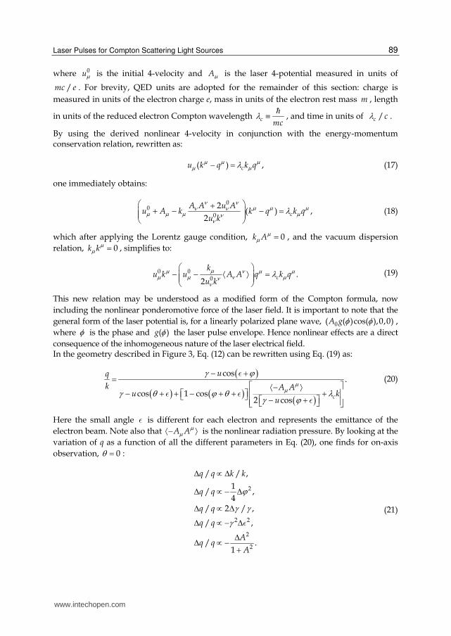
Currently, Compton scattering is among the only physical processes capable of producing a narrow bandwidth radiation (below 1%) at gamma-ray energies, using state-of-the art accelerator and laser technologies. In Compton scattering light sources, a short laser pulse and a relativistic electron beam collide to yield tunable, monochromatic, polarized gamma-ray photons. Several projects have recently utilized Compton scattering to conduct NRF experiments: Duke University2, Japan3 and Lawrence Livermore National Laboratory (LLNL)4. In particular, LLNL's Thomson-Radiated Extreme X-rays (T-REX) project demonstrated isotope specific detection of low-Z and low density materials (7Li) shielded behind high-Z and high-density materials (Pb, Al). The T-REX device and the MEGa-ray machine currently in progress at LLNL are laser-based Compton sources that produce quasi-monochromatic, tunable, polarized gamma-rays via Compton scattering of energetic short duration laser pulses from high-brightness relativistic electron bunches. The detection of low-Z and low-density objects shielded by a high-Z dense material is a long-standing problem that has important applications ranging from homeland security and nonproliferation5 to advanced biomedical imaging and paleontology. X-rays are sensitive to electron density, and x-ray radiography yields poor contrast in these situations. Within this context, NRF offers a unique approach to the so-called inverse density radiography problem. Since NRF is a process in which nuclei are excited by discrete high-energy (typically MeV) photons and subsequently re-emit gamma-rays at discrete energies determined by the structure of the nucleus, and the resonance structure is determined by the number of neutrons and protons present in the nucleus, NRF provides isotope-specific detection and imaging capability6. Thus Compton sources have a lot of potential high profile applications, since NRF can be used for nuclear waste assay and management, homeland security and stockpile stewardship, among others. Other processes and physics can be investigated with narrowband gamma-rays, such as near-threshold photofission, giant dipole resonances, and detailed studies of nuclear structure. This chapter presents, primarily within the context of NRF-based applications, the theoretical and experimental aspects of a mono-energetic gamma-ray Compton source. In Section 2, we will introduce the fundamental concepts and basic physics involved in Compton scattering. In Section 3, we will discuss concepts necessary for understanding laser technology underlying high brightness Compton sources. Section 4 will cover amplification applications and review of some laser pulse measurement techniques. Nonlinear conversion will be discussed in Section 5. Finally, Section 6 contains descriptions of some simulation tools.

2. Mechanics of compton scattering

An electromagnetic wave that is incident upon a free charged particle will cause it to oscillate and so emit radiation. The accelerated motion of a charged particle will generate radiation in directions other than that of the incident wave. This process may be described as Compton scattering of the incident radiation. In this section, we will review the elementary physics of this interaction.

2.1 Overview

Consider an electromagnetic wave with the electric field 0ˆ cos( )E t E e k x is incident

upon a charged particle of charge e and mass m. Assuming that the resultant motion of the

www.intechopen.com

Laser Pulses for Compton Scattering Light Sources 85

charge is nonrelativistic, the particle acceleration is e

mx E . Such an accelerated motion will

radiate energy at the same frequency as that of the incident wave. The power radiated per unit solid angle in some observation direction q can be expressed in the cgs system of units as

22 220

2ˆ ˆ .

4

cEdP e

d mc e q (3)

From a scattering perspective, it is convenient to introduce a scattering cross section, defined by

Energy radiated/unit solid angle/unit time

Incident energy flux/unit area/unit time

d

d

(4)

where the incident flux is 20 / 4S cE . Thus the scattering cross section is

220

1 ˆ ˆd dPr

d S d

e q (5)

where 2 20 /r e mc is the classical electron radius. The result in Eq. (5) is valid for radiation

polarized along a specific direction e . For unpolarized incident radiation, the scattering cross section is

220 1 cos

2

rd

d

(6)

where is the scattering angle between the incident k and scattered q directions. The total scattering cross section obtained by integration over all solid angles is

2 25 20

86.65 10

3T r cm (7)

or better known as the Thomson cross section. The Thomson cross section is only valid at low energies where the momentum transfer of the radiation to the particle can be ignored and the scattered waves has the same frequency as the incident waves. In 1923, Arthur Compton at Washington University in St. Louis found that the scattered radiation actually had a lower frequency than the incident waves. He further showed that if one adopts Einstein’s ideas about the light quanta, then conservation laws of energy and momentum in fact led quantitatively to the observed frequency of the scattered waves. In other words, when the photon energy approaches the particle’s rest energy 2mc , part of the initial photon momentum is transferred to the particle. This would become known as the Compton effect. For this effect to be neglected, we must have

2mc in the frame where the charged particle is initially at rest. If this condition is violated, important modifications to Eq. (6) must be made due to the Compton effect. Quantum electrodynamical calculations give the modified scattering cross section for unpolarized radiation, in the initial rest frame of the charged particle,

www.intechopen.com


22

20 sin2

rd

d

(8)

where and are the incident and scattered frequencies, respectively. They are related by the Compton formula:

2

1

1 1 cosmc

(9)

The total cross section for scattering is then modified to

20 3 2

2 1 ln 1 21 1 32 ln 1 2

1 2 2 1 2KN r

(10)

where 2/mc is the normalized energy of the incident light. This is called the Klein-Nishina cross section, first derived by Klein and Nishina in 1928. For 1 , Eq. (8) reduces to the Thomson cross section of Eq. (6). For scattering by high energy photons, the total cross section decreases from the Thomson value, as shown in Figure 1.

Fig. 1. Plot of the Klein-Nishina expression for the Compton scattering cross section. For small values of , the Compton cross section approaches the Thomson limit. At large values of , the Compton cross section approaches the asymptotic solution 3 1

8 2~ (ln 2 )T

KN .

While the scattering expressions are simple in the frame where the particle is initially at rest, it is often desirable to do calculations in the laboratory frame where the electromagnetic

www.intechopen.com


fields are experimentally measured. To facilitate this, we will need generalizations of Eqs. (8) and (9) valid in an arbitrary inertial frame. The expressions are well known but their derivation is slightly involved, so we will simply quote the results7:

22

022 ˆ2 1

r Xd

d

β k

(11)

ˆ1

ˆˆ ˆ1 1

β k

β q k q

(12)

where β is the initial particle velocity and 2

1

1 . The spin-averaged relativistic

invariant X can be expressed as

21

1 22

p p p pX

(13)

where k p , q p are products of the 4-vectors / ,k c k , / ,q c q and ,p mc β ; and are the incident and scattered 4-polarizations, respectively; p p k q is the 4-momentum of the charged particle after the scattering event. When the photon polarizations are not observed, this expression must be summed over the final and averaged over the initial polarizations, giving

22 2 2 2 2 2 2 21

22 pol

m c m c m c m cX X

(14)

The above describes the interaction of a single electron with an incident electromagnetic wave. For realistic laser-electron interactions, one needs to take into account the appropriate photon and electron phase space. The most useful expression to describe the source is typically the local differential brightness, which may be written in terms of the number of scattered photons, N, per unit volume per unit time per solid angle per energy interval8:

6

3 33 0( ) e

p kd dq q n n d d

d m kdqd d xd

N

t

p k

(15)

where 3en d p and 3n d k represent the electron beam phase space density and laser photon

phase space density, respectively. The factor p k

m k

represents the relative velocity between

the electron and photon and is equal to c for 1 . The delta function in 0q q is required

simply to preserve energy-momentum conservation relation expressed in Eq. (12). Let us briefly apply some of theory discussed above to a realistic Compton source. Consider a Compton scattering geometry in Figure 2. Here, 0m cp u . Let us assume 1 , it is

www.intechopen.com


evident from Eq. (12) that the scattered photon energy maximizes for on-axis scattering events, with , 0 . For a relativistic electron with 1 , we may use the

approximation, 2

11

2 , and find that Eq. (12) simplifies to 24

. In the case of

highly relativistic electrons, the scattered radiation can be many orders of magnitude more energetic than the incident radiation! One can intuitively understand why this occurs. The counter-propagating incident radiation in the electron rest frame is up-shifted by a factor 2 due to the relativistic Doppler effect. The scattered radiation is emitted at approximately the same energy in the electron frame. The Lorentz transformation back to the laboratory frame gives another factor of 2 . Using typical experimental values for an interaction laser

operating at 532 nm, 2.33 eV, colliding head-on with a relativistic electron with

227 , we find that /

0.0021

which justifies neglecting the Compton effect to first

order. More importantly, the scattered radiation will have energy 2 54 4.8 10 eV which is well within the gamma-ray regime. The electron energy is decreased by a corresponding amount.

Fig. 2. Definition of the Compton scattering geometry in the case of a single incident electron.

2.2 Spectral broadening mechanisms

In the case of a weakly focused laser pulse (typical for Compton scattering sources), the coordinates of the wavevector ( , , )x y zk k k remain close to their initial values 0(0,0, )k .9 The exact nonlinear plane wave solution for the 4-velocity has been derived in earlier work10,11:

0 0

0

( 2 )

2

A A uu u A k

k u

(16)

www.intechopen.com


where 0u is the initial 4-velocity and A is the laser 4-potential measured in units of

/mc e . For brevity, QED units are adopted for the remainder of this section: charge is measured in units of the electron charge e, mass in units of the electron rest mass m , length

in units of the reduced electron Compton wavelength cmc

, and time in units of /c c .

By using the derived nonlinear 4-velocity in conjunction with the energy-momentum conservation relation, rewritten as:

( ) ,cu k q k q (17)

one immediately obtains:

0

00

2( )

2,c

A A u Au A k k q k q

u k

(18)

which after applying the Lorentz gauge condition, 0k A , and the vacuum dispersion relation, 0k k , simplifies to:

0 00

.2

c

ku k u A A q k q

u k

(19)

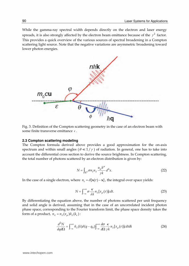
This new relation may be understood as a modified form of the Compton formula, now including the nonlinear ponderomotive force of the laser field. It is important to note that the general form of the laser potential is, for a linearly polarized plane wave, 0( ( )cos( ),0,0)A g , where is the phase and ( )g the laser pulse envelope. Hence nonlinear effects are a direct consequence of the inhomogeneous nature of the laser electrical field. In the geometry described in Figure 3, Eq. (12) can be rewritten using Eq. (19) as:

cos

.

cos 1 cos2 cos c

uq

k A Au k

u

(20)

Here the small angle is different for each electron and represents the emittance of the electron beam. Note also that A A is the nonlinear radiation pressure. By looking at the variation of q as a function of all the different parameters in Eq. (20), one finds for on-axis observation, 0 :

2

2 2

2

2

/ / ,

1/ ,

4/ 2 / ,

/ ,

/ .1

q q k k

q q

q q

q q

Aq q

A

(21)

www.intechopen.com


While the gamma-ray spectral width depends directly on the electron and laser energy

spreads, it is also strongly affected by the electron beam emittance because of the 2 factor. This provides a quick overview of the various sources of spectral broadening in a Compton scattering light source. Note that the negative variations are asymmetric broadening toward lower photon energies.

Fig. 3. Definition of the Compton scattering geometry in the case of an electron beam with some finite transverse emittance .

2.3 Compton scattering modeling The Compton formula derived above provides a good approximation for the on-axis spectrum and within small angles ( 1 / ) of radiation. In general, one has to take into account the differential cross section to derive the source brightness. In Compton scattering, the total number of photons scattered by an electron distribution is given by:

4

4 .eR

u kN n n d x

k

(22)

In the case of a single electron, where [ ( ) ]en x x , the integral over space yields:

[ ( )] .N n x cdtk

(23)

By differentiating the equation above, the number of photons scattered per unit frequency and solid angle is derived, assuming that in the case of an uncorrelated incident photon phase space, corresponding to the Fourier transform limit, the phase space density takes the form of a product, ( ) ( )n nn x k :

0

2

( ) ( ) [ ( )]d N d

n k q q n x cdtdkdqd d k

(24)

www.intechopen.com


The quantity /d d is the differential cross-section in Eq. (11). In turn, the integral over k can be formally performed to obtain

0

2 ( )[ ( )] .

/pk k

n kd N dn x cdt

dqd d k dq dk

(25)

For a Gaussian laser pulse, the photon density in the Fourier domain is

2

01exp

k kn

kk

(26)

and the incident photon density can be modeled analytically within the paraxial approximation, and in the case of a cylindrical focus:

2 2

3/2 2 2 2 20 0 0 0

1 /( , ) exp 2 2 ,

( / 2) 1 ( / ) [1 ( / ) ]

N t z c rn t

tw c t z z w z z

x (27)

where N is the total number of photons in the laser pulse, t the pulse duration, 0w the 21 / e focal radius and 2

0 0 0/z w is the Rayleigh range. To evaluate the integral in Eq. (25), we replace the spatial coordinates by the ballistic electron trajectory:

0

0

0

2 2 2

( )

( )

( )

( ) ( ) ( )

x

y

z

ux t x ct

uy t y ct

uz t z ct

r t x t y t

(28)

where we can divide x, y and r by 0w and z and ct by 0z to obtain the normalized quantities x , y , z , r and t . One finally obtains the expression:

2 20( ) /

3

2

20

2 220

2 2

1

| ( )| / 2

1exp 2 ( ) 2 .

1 1

p

k k k

k ck k

Nd N d e

dqd d k q kk w c t

z rt z dt

c tz z

(29)

Example spectra for the photon source developed at LLNL are shown in Figure 4. It also shows the importance of considering recoil in the case of narrowband gamma-ray operation. The Klein-Nishina formalism presented above is well-suited to model recoil, but does not take into account nonlinear effects. Within the context of laser-plasma and laser electron interactions, nonlinear effects are neglected unless the normalized laser potential A approaches unity. A A A is most commonly described in practical units:

www.intechopen.com


10 1/208.5 10A I , where 0 is the laser wavelength measured in m and I the laser

intensity in units of 2/W cm . Typically, 0.1A or less for today’s Compton sources. It has been shown that, despite being in a regime where 2 1A , nonlinear effects can strongly increase the width of the gamma-ray spectra11.

Fig. 4. Gamma-ray spectra in the case of Compton scattering (black) and Thomson scattering (blue). Left: T-REX source parameters (laser: 20 ps FWHM pulse duration, 532 nm wavelength, 34 μm rms spot size, 150 mJ; electron beam: 116 MeV, 40 μm rms spot size, 20 ps FWHM bunch length, 0.5 nC beam charge, 6 mm.mrad normalized emittance). Right: future Compton source parameters (laser 10 ps FWHM pulse duration, 532 nm wavelength, 12 μm rms spot size, 150 mJ; electron beam: 250 MeV, 15 μm rms spot size, 10 ps FWHM bunch length, 0.25 nC beam charge, 1 mm.mrad normalized emittance).

For completeness, we will briefly describe an alternative formalism based on classical radiation theory. Nonlinear spectra can also be calculated from the electron trajectories by using the covariant radiation formula that describes the number of photons scattered per unit frequency and solid angle:

2

(2

2)( )

4iq xd N

e ddqd

cq

q u (30)

where is the fine structure constant, ( , )q q q the scattered 4-wavenumber and / ( , )u dx cd u the electron 4-velocity along its trajectory. Eq. (17) can be generalized

to describe the scattering process for nonlinear, three-dimensional, and correlated incident radiation. On the other hand, Eq. (25) properly satisfies energy-momentum conservation, therefore accounting for recoil, and also includes QED corrections when using the Klein-Nishina differential scattering cross-section. The two approaches yield complementary information, but are mutually incompatible, and coincide only for Fourier transform-limited (uncorrelated) plane waves in the linear regime and in the limit where 0c . Returning to Eq. (24) and comparing it with Eq. (30), it is clear that the quantities /d d and

2q u

www.intechopen.com


play equivalent roles, and the Dirac delta-function 0( )q q is related to the Fourier transform in the case of an infinite plane wave. Using Eq. (30), important modifications to the radiation spectrum under strong optical fields using the classical radiation formula have been predicted. The interested reader may peruse Refs. 9 and 11 for more details.

3. Laser technology

This chapter describes some of the main concepts necessary for understanding laser technology underlying high brightness, Compton scattering based mono-energetic gamma-ray sources. Using the recently commissioned T-REX device at LLNL as a model12,13, the two main components are a low emittance, low energy spread, high charge electron beam and a high intensity, narrow bandwidth, counter-propagating laser focused into the interaction region where the Compton scattering will occur. A simplified schematic of the Compton-scattering source is shown in Figure 5. The laser systems involved are among the current state-of-the art.

Fig. 5. Block diagram of the LLNL MEGa-ray Compton source with details of the laser systems.

An ultrashort photogun laser facilitates generation of a high charge, low emittance electron beam. It delivers spatially and temporally shaped UV pulses to RF photocathode to generate electrons with a desired phase-space distribution by the photoelectric effect. Precisely synchronized to the RF phase of the linear accelerator, the generated electrons are then accelerated to relativistic velocities. The arrival of the electrons at the interaction point is timed to the arrival of the interaction laser photons. The interaction laser is a joule-class, 10 ps chirped pulse amplification system. A common fiber oscillator, operating at 40 MHz repetition rate, serves as a reference clock for the GHz-scale RF system of the accelerator, seeds both laser systems and facilitates sub-picosecond synchronization between the interaction laser, the photogun laser, and the RF phase. Typical parameters for the laser system are listed in Table 1. To help understand the function and the construction of these laser systems, this chapter we will provide a brief overview of the key relevant concepts, including mode-locking, chirped-pulse amplification, nonlinear frequency generation, laser diagnostics and pulse characterization techniques. We will also describe the most common laser types involved in

www.intechopen.com


generation of energetic ultrashort pulses: solid state Nd:YAG and Titanium:Sapphire, and fiber-based Yb:YAG.

Parameters Oscillator Photogun Laser Interaction Laser

Repetition Rate 40.8 MHz 10-120 Hz 10-120 Hz Wavelength 1 μm 263 nm 532 nm or 1 μm Pulse Energy 100 pJ 30-50 μJ 150 mJ - 800 mJ Pulse Duration 1 ps 2 or 15 ps 10 ps Spot size on target n/a 1-2 mm 20-40 μm RMS

Table 1. Summary of key laser parameters for T-REX and MEGa-ray Compton scattering light source.

3.1 Chirped pulse amplification Chirped pulse amplification, invented over two decades ago14, allow generation of highly energetic ultrashort pulses. The key concept behind CPA is to increase the pulse duration prior to amplification, thereby reducing the peak intensity during the amplification process. The peak intensity of the pulse determines the onset of various nonlinear processes, such as self-focusing, self-phase modulation, multi-photon ionization that lead to pulse break-up and damage to the amplifying medium. A measure of nonlinear phase accumulation, the “B-integral”, is defined by:

22

( )NL n I z dz

(31)

where ( )I z is a position dependent pulse intensity and 2n is the material dependent nonlinear refractive index ( 0 2n n n I ). NL should normally be kept below 2-3 to avoid significant pulse and beam distortion. For a desired final pulse intensity, we minimize the value of the accumulated B-integral by increasing the beam diameter and the chirped pulse duration. After amplification, the stretched pulse is recompressed to its near transform limited duration. The four stages of the CPA process are illustrated in Figure 6.

Fig. 6. Basic CPA scheme: ultrashort seed pulse is stretched, amplified, and recompressed.

The seed pulse in any CPA system is produced by an ultrashort oscillator. Typically, the pulse energy from a fiber oscillator is in the 10 sec of pico-Joule range, and 10 sec of nJ from a solid-state oscillator. The oscillator pulse is then stretched in time and amplified. Depending on the system, pulse stretching can occur in a bulk grating stretcher, prism-based stretcher, chirped fiber Bragg grating, or chirped volume Bragg grating. Stretching and amplification can occur in several stages depending on the final energy. Initial pre-amplifiers provide very high gain (up to 30 dB or more is possible) to boost the pulse energy

www.intechopen.com


to mJ levels. Power amplifiers then provide lower gain but higher output energy. Many amplifier stages can be multiplexed. State of the art custom systems can produce over 1 PW of peak power, corresponding to for example 40 J in 40 fs.15,16 Many implementations of the chirped pulse amplification have been demonstrated. Typically, amplifiers consist of high bandwidth laser gain medium, such as Ti:Sapphire or Yb:YAG. The laser crystal is pumped by an external source to produce population inversion prior to the arrival of the seed pulse. The seed pulse then stimulates emission and grows in energy. In another amplification scheme, called optical parametric chirped pulse amplification (OPCPA), no energy is stored in the medium. Instead, gain is provided through a nonlinear difference frequency generation process. A very high quality, energetic narrowband pump laser is coincident on a nonlinear crystal at the same time as the chirped seed pulse. The seed pulse then grows in energy through a parametric three-photon mixing process. The advantage of this scheme is that no energy is stored in the medium and the nonlinear crystal is much thinner compared to a laser crystal. Hence, thermal management and nonlinear phase accumulation issues are mitigated in OPCPA. A key difficulty to implementing OPCPA, is that the pump laser has to be of very high quality. After the amplification stage, pulses are recompressed in a pulse compressor. For joule class final pulses, recompression occurs exclusively in grating based compressors. Detailed dispersion balance is required to produce a high fidelity final pulse. Details of pulse stretchers and compressors are provided in the following section.

3.2 Pulse stretching and compressing

The action of various dispersive elements is best described in the spectral domain. Given a time dependent electric field, 0( ) ( ) i tE t A t e , where we factor out the carrier-frequency term, its frequency domain is the Fourier transform:

( )( ) ( ) ( ) ii tsA t e dt I e

. (32)

Here, we explicitly separate the real spectral amplitude ( )sI , and phase ( ) . We define spectral intensity

2( ) ( )sI , and temporal intensity

2( ) ( )I t A t We can Taylor expand

the phase of the pulse envelope ( ) as

( )

0

1( ) (0)

!n n

n n

(33)

where ( ) ( )(0)

nn

n

d

d

evaluated at 0 . The 1n term is the group delay,

corresponding to the time shift of the pulse; terms 2n are responsible for pulse

dispersion. The terms ( )(0)n , where 2n and 3, are defined as group delay dispersion

(GDD) and third order dispersion (TOD), respectively. For an unchirped Gaussian pulse, 2

20

0( )

t

E t E e , we can analytically calculate its chirped duration, f assuming a purely

quadratic dispersion ( ( )(0) 0n for 2n ).

www.intechopen.com


2

0 40

1 16f

GDD (34)

The transform limited pulse duration is inversely proportional to the pulse bandwidth. For a transform limited Gaussian, the time-bandwidth product (FWHM intensity duration [sec] × FWHM spectral intensity bandwidth [Hz]) is 2 log 2 0.44 . From Eq. (34), for large stretch ratios, the amount of chirp, GDD, needed to stretch from the transform limit, 0 , to the final duration, f , is proportional to 0 . In our CPA system, a near transform limited pulse is chirped from 200 fs (photogun laser) and 10 ps (interaction laser) to a few nanosecond duration. Options for such large dispersion stretchers include chirped fiber Bragg gratings (CFBG), chirped volume Bragg gratings (CVBG), and bulk grating based stretchers. Prism based stretchers do not provide sufficient dispersion for our bandwidths. The main attraction of CFBG and CVBG is their extremely compact size and no need for alignment. Both CFBG and CVBG have shown great recent promise but still have unresolved issues relating to group delay ripple that affect recompressed pulse fidelity17. High pulse contrast systems typically utilize reflective grating stretchers and compressors which provide a smooth dispersion profile. Grating stretchers and compressors are guided by the grating equation which relates the angle of incidence and the angle of diffraction measured with respect to grating normal for a ray at wavelength ,

sin sinm

d

(35)

where d is the groove spacing and m is an integer specifying the diffraction order. Grating stretchers and compressors achieve large optical path differences versus wavelength due to their high angular resolution18,19. A stretcher imparts a positive pulse chirp (longer wavelengths lead the shorter wavelengths in time) and a compressor imparts a negative pulse chirp. The sign of the chirp is important, because other materials in the system, such as transport fibers, lenses, and amplifiers, have positive dispersion. A pulse with a negative initial chirp could become partially recompressed during amplification and damage the gain medium. The dispersion needs to be balanced in the CPA chain to recompress the pulse to its transform limit. The total group delay, totalGD versus wavelength for the system must be a constant at the output, or

1

( ) ( ) ( ) ( )

( ) ( ) ( )

total stretcher compressor fiber

oscillator amplifier material

GD GD GD GD

GD GD GD C

(36)

where 1C is an arbitrary constant. From Eq. (33), ( ) ( )GD d . Any frequency

dependence in the total group delay will degrade pulse fidelity. Several approaches to achieving dispersion balance exist. In the Taylor expansion (Eq. (33)) to the phase of a well behaved dispersive elements, when n m the contribution of a term n to the total phase is much larger than of a term m, or ( ) ( )(0) / ! (0) / !n mn mn m ,

www.intechopen.com


where is the pulse bandwidth. One approach to achieve dispersion balance is to calculate the total GDD, TOD, and higher order terms for the system and attempt to zero them. For example, when terms up to the 4th order are zero, the system is quintic limited. This term-by-term cancellation approach can become problematic when successive terms in the Taylor expansion do not decrease rapidly. It is often preferable to minimize the residual group delay, RMSGD , over the pulse bandwidth,

2 2

2

( ) ( )

( )RMS

GD GD dGD

d

(37)

where GD is the mean group delay defined as

2

2

( ) ( )

( )

GD dGD

d

. (38)

A sample pulse stretcher is shown in Figure 7. The stretcher consists of a single grating, a lens of focal length f, a retro-reflecting folding mirror placed f away from the lens and a vertical roof mirror. The folding mirror simplifies stretcher configuration and alignment by eliminating a second grating and lens pair. A vertical roof mirror double passes the beam through the stretcher and takes out the spatial chirp. The total dispersion of the stretcher is determined by the distance from the grating to the lens, fL . When fL f , the path lengths at all wavelengths are equal and the net dispersion is zero. When fL f , the chirp becomes negative, same as in the compressor. In a stretcher, fL f producing a positive chirp. We can calculate the dispersion, or ( ) ( ) /GD n L c , where ( )L is the frequency dependent propagation distance and n is the frequency dependent refractive index, using various techniques.

Fig. 7. Grating and lens based stretcher is folded with a flat mirror. The distance from the grating to the focal length of the lens determine the sign and magnitude of the chirp.

Here, we give a compact equation for ( )

( )GD

GDD

, from which all other dispersion

terms can be determined. Assuming an aberration free stretcher in the thin lens approximate, ( )GDD is then given by

2

2 2

sin sin( ) 2( )

cosfGDD f L

c

(39)

www.intechopen.com


where the diffraction angle, is a function of . The aberration free approximation is important, because a real lens introduces both chromatic and geometric beam aberrations which modify higher order dispersion terms from those derived from Eq. (39). A compressor, which is typically a final component in the CPA system, undoes all of the system dispersion. The compressor used on the photogun laser is shown in Figure 8. Compared to the stretcher, the lens is absent. The magnitude of the negative chirp is now controlled by the distance from the horizontal roof to the grating. The horizontal roof, here folds the compressor geometry and eliminates a second grating. As in the stretcher of Figure 7, the compressor’s vertical roof mirror double passes the beam and removes the spatial chirp. Because a compressor has no curved optics, it introduces no geometric or chromatic aberrations. The dispersion of a real compressor is very precisely described by the Treacy formula or its equivalent given by

2

1 2 2

sin sin( )

cosGDD L

c

(40)

The actual stretcher design for MEGa-ray photogun laser is shown in Figure 9. The all-reflective Offner design uses a convex and a concave mirror to form an imaging telescope with magnification of -1 and relay planes at the radius of curvature (ROC) center of the concave mirror20. The grating is placed inside the ROC to impart a positive chirp. A vertical

Fig. 8. Folded grating compressor. The distance from the horizontal roof mirror to the grating determines the magnitude of the negative chirp.

Fig. 9. Raytraced design of the Offner stretcher for the photogun laser.

www.intechopen.com


roof mirror folds the stretcher geometry and eliminates the second grating. The Offner stretcher is compact and has low chromatic and geometric aberrations. Consequently, its dispersion profile is nearly aberration free, meaning the GDD and higher order dispersion terms are closely predicted by Eq. (39).

3.3 Ultrashort oscillators Essential to building a high energy ultrashort laser system is a highly stable, robust oscillator. The oscillator serves as a front end, seeding an amplifier chain. Modelocking process generates pulses with duration from few picoseconds down to few femtoseconds. Modelocking is at the heart of all ultrashort laser systems. Some more exotic nonlinear techniques have generated few femtoseconds pulses without utilizing modelocking21,22; however, these are still at a laboratory research stage. The basic idea of modelocking consists of adjusting the relative phases of all the cavity laser modes to be in-phase. The phase adjustment occurs either passively or actively. Consider a simple two mirror cavity of length L. Confining our discussion to TEM00 modes, the allowed mode spacing in the frequency domain is / 2 gc n L , where c is the speed of

light and gn is the group refractive index, ( )g

nn n

. is also known as the free

spectral range (FSR). For higher order modes, the frequency spacing is slightly modified because the Guoy phase shift increases with mode number. While the mode spacing is typically in the few GHz to 100s of MHz range, the total bandwidth for 100 fs pulse ≈10 THz. This results in ≈10000 laser modes in the cavity. In the time domain, total electric field can be expressed as

1

1( ) exp( ) . .

2

N

q q qq

E t E i t i c c

(41)

where the sum is taken over all N modes, and is the phase associated with each mode. When all the phases are equal, the pulse intensity is a periodic function with pulse to pulses spacing given by 1 / . Assuming Gaussian pulses, the pulse width becomes

0.44 /t N , where t is the 21 / e pulse duration and N is equivalent to 21 / e pulse bandwidth. The idea behind modelocking consists of introducing a variable cavity loss condition. The cavity loss is engineered so that the pulse with the highest intensity will experience the smallest loss. The modelocking mechanism can be either passive or active. In active modelocking, an active element, such as an acousto-optic or an electro-optic modulator periodically modulates the cavity loss. In the time domain, the modulator acts as a shutter which lets light through only when it is open. Using a fast modulator synchronized to the cavity roundtrip time, we can obtain pulses as short as a few picoseconds. This type of mechanism is known as amplitude modulation (AM) modelocking. Active modelocking can also occur by modulating the phase of the light with an electro-optic phase modulator. The idea, here, is that light passing through a phase modulator acquires sidebands at upshifted and downshifted frequencies. When the frequency shifted sidebands are outside the gain bandwidth of the laser medium, they are attenuated after many roundtrips. When the phase modulator is synchronized with the cavity roundtrip

www.intechopen.com


time, only the sidebands which pass through the modulator at zero frequency shift will be amplified. Therefore, a short pulse experiences the largest gain. For a homogeneous laser, the primary mechanism that limits pulse duration of an actively modelocked laser is gain narrowing. The pulse duration, p can be calculated for a steady state case by23

1/21/41

0.45pm m g

G (42)

where G is the roundtrip gain, m is the modulation depth, m is the modulation frequency, and g is the FWHM gain bandwidth. From this equation, the highest modulation frequency limits the final pulse duration. Pulses shorter than a few picoseconds are difficult to generate using this technique because of the limit on the driving electronics. In contrast to active modelocking, passive modelocking does not involve external modulation, and can produce pulses as short as ≈5 fs. The basic idea, here, is to use a saturable absorber inside the cavity. The saturable absorber has a loss which decreases with intensity. Hence, the highest intensity pulses experience the largest cavity gain. A saturable absorber can also be described as a very fast shutter, much faster than an actively driven device. Implementation of the saturable absorber takes several forms. Bulk lasers typically rely on either a semiconductor saturable absorber mirror (SESAM) or on Kerr-lens modelocking (KLM). A SESAM is a multi-layer semiconductor device which reflects light due to Bragg reflections off the periodic structure. A thin absorbing top layer saturates with intensity, increasing the mirror reflectivity. SESAM structures are used on various types of diode pumped ultrashort laser operating in the 1 μm and longer spectral range. The shortest pulses to date are generated with Ti:Sapphire systems and rely on Kerr-lens modelocking. Kerr lensing is a third-order nonlinear effect due to intensity dependence of the refractive index, 0 2n n n I , where I is the pulse intensity. The intensity dependence of the refractive index leads to beam self-focusing when 2 0n . The nonlinear medium acts as a positive lens. Inside an oscillator, this implies that the spatial mode of a short pulse is smaller than the spatial mode of the longer pulse. By introducing a small aperture, we can filter out the larger spatial modes. The modelocked pulse will then experience the largest gain in the resonator. Finally, ultrashort fiber lasers have generated sub 100 fs pulses. Fibers lasers are highly portable, reliable, relatively insensitive to external perturbations, provide long term hands free operation, and can scale to average powers above 1 kW in a diffraction limited beam and CW operation24. For many applications, ultrashort fiber oscillators are replacing traditional solid-state systems. For example, on T-REX we employ a 10 W Yb:doped mode-locked oscillator which, when compressed, produces 250 pJ, sub 100 fs, near transform limited pulses at 40.8 MHz repetition rate with a full bandwidth from 1035 nm to 1085 nm. The oscillator, based on a design developed at Cornell25, fits on a rack mounted, 12"×12" breadboard (see Figure 10). An example of the oscillator spectrum from the LLNL fiber oscillator is shown in Figure 11. The passively modelocked fiber oscillator is based on a type of saturable absorber process called nonlinear polarization evolution26. Nonlinear polarization evolution is a nonlinear process also based on the intensity dependence of the refractive index. Inside a non polarization maintaining fiber, two orthogonally polarized

www.intechopen.com


Fig. 10. The ultrashort Yb+ doped fiber oscillator fits on a 12”x12” breadboard. When recompressed, the anomalous dispersion oscillator generates 100 fs pulses.

Fig. 11. Experimental pulse spectrum of the MEGa-ray oscillator of Figure 10. The same oscillator seeds both the interaction and the photogun lasers.

www.intechopen.com


electric fields will experience different intensity dependent phase shifts, rotating the final polarization state. When a polarizer is placed at the output, the polarization rotation is converted to amplitude modulation. By properly selecting the length of the gain fiber and adjusting the input and output polarization state, we can produce a modelocked pulse. The fiber oscillator cavity also contains a pulse compressor which disperses the circulating pulse. The pulse compressor partially compensates for fiber dispersion. The output modelocked pulse from a fiber oscillator is typically slightly chirped.

4. Amplification of laser pulses

A laser amplifier coherently boosts the energy of the input pulse. In a standard master oscillator power amplifier (MOPA) configuration, a picojoule scale seed pulse from the oscillator can be amplified to Joule scale and above. The most extreme example is the laser at the National Ignition Facility, where a few nanojoule oscillator is amplified to a final pulse energy of 10 kJ.27 The action of the amplifier is illustrated in Figure 12. An input pulse with intensity inI is amplified to output intensity outI . An amplifier can be characterized by its small signal (undepleted) gain, 0G , saturation fluence, satJ , and its frequency dependent lineshape function, ( )g . In general, we need to solve the laser rate equations to determine the output pulse shape, spectral distribution, and energy. For a homogeneous gain medium, when (1) the temporal pulse variation and the population inversion is sufficiently slow (compared to 2T coherence time) to justify rate equation analysis, and (2) transient effects relating to spontaneous emission and pumping occur on a time scale much longer than the pulse duration, an analytical solution can be obtained using a Frantz-Nodvik approach28. Eq. (43) is derived for a monochromatic input pulse29.

1( )/ ( )1

0( ) ( ) 1 1 in satJ t J tout inI t I t G e

(43)

Here, 0

( ) ( )t

in inJ t I t dt is the instantaneous fluence. Eq. (43) can be modified to describe

amplification of a chirped pulse. This involves determining the frequency dependence of the small gain, 0( )G and the saturation fluence, ( )satJ , both of which depend on the emission

cross-section ( )e . For a four-level system, ( ) / ( )sat eJ h , and 0 exp ( )eG N ,

where N is the population inversion. If the instantaneous pulse frequency, 1 ( )

2

d t

dt

is a

monotonic function of t, we can define time as a function of frequency, ( )t . In this

instantaneous frequency approach, we can rewrite Eq. (43) as a function of . Various aspects of chirped pulse amplification, such as total output energy, gain narrowing, square pulse distortion, and spectral sculpting can be analytically calculated using the modified form of Eq. (43). A major constraint on the ultrashort pulse amplifier is that the gain medium must be sufficiently broad to support the required pulse duration. To illustrate the operation of the ultrashort oscillator combined with an amplifier, we use the T-REX laser system. A single fiber oscillator seeds both, the photogun laser and the interaction laser systems. An experimental oscillator spectrum showing the bandpass for the photogun and the

www.intechopen.com


interaction lasers is shown in Figure 11. Two different chains of fiber Yb:doped fiber amplifiers tuned for peak gain at 1053 nm for PDL and 1064 nm for ILS, boost the seed pulse to ≈100 μJ/pulse. The seed is chirped to a few nanosecond duration prior to amplification. Each fiber amplifier stage provides 20 dB of gain. The repetition rate is gradually stepped down to 10 kHz with acousto-optic modulators (AOM), inserted in between fiber amplifiers. The AOMs also remove out of band amplified spontaneous emission (ASE), preserving pulse fidelity.

Fig. 12. Basic scheme for pulse amplification. A gain medium with stored energy coherently amplifies the input pulse.

The total energy from the fiber amplifier is limited by the total stored energy and by the accumulated nonlinear phase in Eq. (31). Several initial amplifier stages consist of telecom-type, 6.6 μm core polarization maintaining (PM) fibers. The output from this core sized fiber is limited to ≈1μJ. Next, a series of large mode field diameter, 29 μm core photonic band-gap (PBG) fibers accommodate pulse energies up to 100 μJ. We are currently developing even larger core (80 μm) PBG fiber rod based amplifiers to attain over 1 mJ per pulse at the output. A major challenge with PBG and other large core fibers is careful control of the refractive index uniformity to prevent generation of higher order spatial modes, which degrade beam quality.

4.1 Introduction to FROG Current electronic bandwidths preclude direct measurement of pulses shorter than ≈50 psec. A wide variety of indirect characterization techniques exist for short pulses produced by mode-locked lasers. Almost exclusively, these methods rely on a nonlinear interaction between two or more pulses. A very common measurement technique is pulse intensity autocorrelation. Here, a signal is measured as a function of delay between the pulse and a replica of the pulse,

( ) ( ) ( )A I t I t dt . (44)

While this method is easy to implement it does not define the actual pulse shape. Different pulse shapes can result in the same autocorrelation trace. Intensity autocorrelation provides a rough measure of the pulse duration, when we assume that the pulse intensity envelope is relatively smooth in time and when spatio-temporal aberrations are absent. To fully characterize a pulse, we must determine the actual electric field profile in time and space ( , , , )E t x y z . An extension of the intensity autocorrelation is interferometric autocorrelation, which involves splitting and recombining the pulse and its replica inside an interferometer. Interferometric stability of the measurement allows the user to resolve the electric field fringes in the measurement. Here the the interferometric autocorrelation signal, IFACA is given by

www.intechopen.com


2

( ) ( )IFACA E t E t dt (45)

Interferometric autocorrelation carries some of the phase information of the field and more accurately resolves the pulse intensity profile. However, no study has shown that the phase information can be fully recovered. Another disadvantage is that interferometric autocorrelation is time consuming to implement and necessarily involves many laser shot sequences. Since the 1990s, several techniques have emerged which characterize both the intensity and the phase of the pulse. One of the best known techniques is Frequency Resolved Optical Grating (FROG)30. In its most simple implementation, a spectrometer is added to the output of the autocorrelator. By measuring the spectral intensity as a function of relative pulse delay we can determine the actual electric field ( )E t of the pulse. The phase information is recovered by applying an iterative algorithm to the measured pulse spectrogram. FROG can be implemented using a variety of nonlinearities. The most common is the 2nd harmonic FROG, where a nonlinear crystal is used in a sum-frequency configuration. Mathematically, it determines

2

( , ) ( ) ( )exp( )SHGFROGI E t E t i t dt

(46)

which is a 2D spectrogram plotting delay versus frequency. Several inversion algorithms exist to process the FROG data and extract pulse intensity and phase. Conceptually, the first pulse ( )E t is a probe, and its replica ( )E t is a gate. In a cross-correlation measurement, the gate pulse should be much shorter than the probe pulse. In practice, however, a shorter pulse is not available and in many cases not required. Many different implementations of the FROG measurement have been implemented utilizing the 3rd order (3) nonlinearity. These include Polarization Gated (PG-FROG), where the nonlinearity is the nonlinear polarization rotation of the probe pulse when mixed with a gate pulse; third harmonic generation (THG-FROG), where the measured signal results from the four-wave mixing process; self-diffraction (SD-FROG) where the signal results when two of the overlapping beams set-up a grating which diffracts portions of both beams along new k-vectors directions. There are various advantages and disadvantages associated with each FROG implementation relating to signal sensitivity, apparatus complexity, potential ambiguities, dynamic range, and ease of analysis. Generally, SHG FROG is best suited for characterization of oscillators and other low intensity pulses. One disadvantage of SHG FROG is a time reversal ambiguity between ( )E t and ( )E t . Both pulses produce identical FROG spectrograms. Hence we need to perform an additional procedure, such as inserting a dispersive element into the beam, to remove this ambiguity. Third order FROG automatically removes the time reversal ambiguity. It also produces FROG spectrograms that more intuitively correspond to actual pulse shapes. FROG measurement can be implemented in a multi-shot configuration, where measurements are performed sequentially and then analyzed, or in a single-shot configuration. In a single-shot configuration, complete pulse information is gathered in a single laser shot. Properly optimized software can provide the pulse shape and phase nearly instantaneously. Similar to single-shot autocorrelation, single shot FROG measurement

www.intechopen.com


interferes one portion of the beam with another portion of the beam. Similar to a streak camera, one of the spatial axes becomes a time axis and a complete spectrogram (spectral intensity versus time and wavelength) is recorded during a single shot. The single-shot FROG techniques are sensitive to spatio-temporal aberrations. Spatio-temporal aberrations refer to temporal differences as a function of position on the beam. A common example includes pulse front tilt, where the pulse arrival time changes across the beam aperture. This can be observed when an ultrashort pulse come off a diffraction grating or passes through a prism. Another spatio-temporal aberration is spatial chirp, where the pulse spectrum varies across the beam aperture. All types of spatio-temporal aberrations can be visualized by representing the pulse as a 3D map, where for example, the spectral intensity is plotted versus position and frequency31. A straight forward single shot FROG implementation using GRENOUILLE can measure both of these types of spatio-temporal aberrations32. Finally, FROG technique is highly robust. Because the pulse information is overdefined, analysis of the recorded FROG traces can uncover certain systematic errors during the measurement process and the measured data set can be checked for self-consistency. The retrieval process is highly visual, as the retrieved spectrogram is easily compared to the recorded spectrogram. While every pulse has a spectrogram, not every spectrogram has an associated electric field. Improperly recorded spectrograms will not result in a retrievable pulse shape. FROG technique is extremely powerful and produces complete electric field information for both simple and ultra-complex shapes. FROG can be implemented for a variety of laser wavelengths from the UV to the IR, and across a wide range of pulse duration, from few femtosecond to 10’s of picoseconds.

4.2 Chirped Pulse Amplification with narrowband pulses In CPA, the gain bandwidth of the amplifying medium is typically broad enough to minimize gain narrowing of the seed pulse. On the photogun laser, Yb doped glass has a wide bandwidth spanning from 1000 nm to 1150 nm, and is well suited for amplifying 100 fs pulses. On the interaction laser, however, bulk amplification is in Nd:YAG, which has a narrow bandwidth of 120 GHz. Nd:YAG technology is a workhorse of high average power lasers. The basic idea is that the gain for a Nd:YAG crystal rod is provided by either flashlamps or laser diodes. Previously, joule-class Nd:YAG amplifiers were flashlamp pumped; recently, however, diode pumped joule-class systems have been introduced commercially. Flashlamp pumping is inefficient compared to diode pumping and causes significant thermal lensing and thermal birefringence in the crystal. As a result, flashlamp pumped rod systems are limited to approximately 10-20 W. Diode pumping significantly reduces the total pump energy, enabling operation at higher repetition rates and higher average power. The diode pumped Nd:YAG based laser system for the next generation gamma-ray source at LLNL is designed to operate at nearly 100 W of average power. Even higher average powers are obtained with slab Nd:YAG amplifiers. Compared to rod geometry, slab geometry is much more efficient at removing the heat from the system. The beam aspect ratio can also be scaled more favorable to reduce unwanted nonlinear effects. However, slab rod geometries are much more difficult to engineer and are not currently commercially viable. Here, we describe an implementation of CPA with Nd:YAG amplifiers. Due to the limited Nd:YAG bandwidth, the seed pulses gain narrow to sub nanometer bandwidths after amplification, sufficient to support 5-10 ps pulse durations. Traditional two-grating stretchers and compressors cannot provide adequate dispersion in a table-top footprint. We

www.intechopen.com


will describe novel hyper-dispersion technology that we developed for CPA with sub-nanometer bandwidth pulses33. The meter-scale stretcher and compressor pair achieve 10x greater dispersion compared to standard two-grating designs. Previously, D. Fittinghoff et al. suggested hyper-dispersion compressor arrangements34. F. J. Duarte described a conceptually similar hyper-dispersion arrangement for a prism-based compressor35. We utilize commercial Nd:YAG amplifiers for two reasons: (1) Nd:YAG technology is extremely mature, relatively inexpensive, and provides high signal gain; (2) nominally 10 ps transform limited laser pulses are well-suited for narrowband gamma-ray generation. Employing a hyper-dispersion stretcher and compressor pair, we generated 750 mJ pulses at 1064 nm with 0.2 nm bandwidth, compressed to near transform limited duration of 8 ps. The nearly unfolded version of the hyper-dispersion compressor is shown in Figure 13, with a retro-mirror replacing gratings 5-8. Compared to standard Treacy design, this compressor contains two additional gratings (G2 and G3). The orientation of G2 is anti-parallel to G1: the rays dispersed at G1, are further dispersed at G2. This anti-parallel arrangement enables angular dispersion, /d d , which is greater than possible with a single grating. The orientation of G3 and G4 is parallel to, respectively, G2 and G1. G3 undoes the angular dispersion of G2 and G4 undoes the angular dispersion of G1 producing a collimated, spatially chirped beam at the retro-mirror. After retro-reflection, the spatial chirp is removed after four more grating reflections. The number of grating reflections (8), is twice that in a Treacy compressor. High diffraction efficiency gratings are essential for high throughput efficiency. We utilize multi-layer-dielectric (MLD) gratings developed at LLNL with achievable diffraction efficiency >99%.36 The magnitude of the negative chirp is controlled by varying L1, the optical path length of the central ray between G1 and G2 and L2, the optical path length between G2 and G3.

Fig. 13. Unfolded version of the hyper-dispersion compressor with anti-parallel gratings.

An analytical formula for group delay dispersion (GDD) as a function of wavelength for the compressor can be derived using the Kostenbauder formalism37,38:

2

221 22 4

sin sin2 cos cos cos

cosGDD L L

c

(47)

Here is the angle of incidence and is the angle of diffraction of the central ray of wavelength at the first grating measured with respect to grating normal. We assume that the groove density of gratings 1 and 2 is the same. Note that the expression for GDD reduces to that of the standard two-grating compressor when 2 0L . Higher order dispersion terms can be derived by noting that is a function of wavelength.

www.intechopen.com


Compressor design can be folded to reduce the total number of gratings and simplify compressor alignment. The compressor shown in Figure 14 has been designed for the MEGa-ray machine and is similar to the experimental design on T-REX. The compressor consists of two 40×20 cm multi-layer dielectric (MLD) gratings arranged anti-parallel to each other, a vertical roof mirror (RM), and a series of two periscopes and a horizontal roof mirror. These six mirrors set the height and the position of the reflected beam on the gratings and invert the beam in the plane of diffraction.

Fig. 14. The compact hyper-dispersion compressor consisting of two 1740 grooves/mm gratings has a footprint of 3x0.7 m and group delay dispersion of -4300 ps2/rad.

The beam is incident at Littrow angle minus 3 degrees (64.8°) on the 1740 grooves/mm gratings. The vertical roof mirror here is equivalent to the retro-mirror in Figure 13. The beam undergoes a total of 8 grating reflections and 16 mirror reflections in the compressor. The total beam path of the central ray is 22 m. On T-REX, the MLD gratings had diffraction efficiency above 97%, enabling an overall compressor throughput efficiency of 60%. Here, the magnitude of the chirp is tuned by translating the horizontal roof mirror. The compressor, with its relatively compact footprint of 3×0.7 m provides

4300GDD ps2/rad, or a pulse dispersion of 7000 ps/nm. This chirps the incident 0.2 nm bandwidth pulse to 3 ns. The two grating separation in a standard Treacy compressor with the same dispersion would be 32 m. The hyper-dispersion stretcher design is conceptually similar. The unfolded version is shown in Figure 15. Compared to the standard Martinez stretcher, the hyper-dispersion design contains two extra mirrors G1 and G4, arranged anti-parallel to G2 and G3. We define fL as the path length from G2 to the first lens. Then the total ray path length from G1 to the first lens, 1 fL L , must be smaller than the lens focal length, f to produce a positive chirp. The magnitude of the chirp is controlled by varying the value of 1 fL L f .

Fig. 15. Unfolded hyper-dispersion stretcher utilizes four gratings, as opposed to two gratings in the standard Martinez design.

We modify Eq. (47) to derive the GDD formula for the aberration free hyper-dispersion stretcher shown in Figure 15:

www.intechopen.com


2

2212 4

sin sincos ( ) cos cos

cosfGDD L L f

c

(48)

The folded CAD version of the stretcher built for T-REX is shown in Figure 16. For high fidelity pulse recompression, the stretcher is designed with a nearly equal and opposite chirp compared to that of the compressor. The small difference accounts for other dispersive elements in the system. We again use two large 1740 grooves/mm MLD gratings, with footprints of 20×10 cm and 35×15 cm. The beam is incident at the same Littrow angle less 3° as in the compressor. A large, 175 mm diameter, 3099f mm lens accommodates the large footprint of the spatially chirped beam. A folding retro-mirror is placed f away from the lens, forming a 2-f telescope seen in the unfolded version of Figure 15. The beam height changes through off-center incidence on the lens. After 4 grating reflections, the beam is incident on the vertical roof mirror, which is equivalent to the retro-mirror in Figure 15. The two 45° mirrors fold the beam path, rendering a more compact footprint. After 8 grating reflections, the compressed pulse arrives and 2nd pass retro-mirror. The beam is then retro-reflected through the stretcher, undergoing a total of 16 grating reflections. We double pass through the stretcher to double the total pulse chirp. Beam clipping on the lens prevents reducing the lens to G2 distance to match compressor dispersion in a single pass.

Fig. 16. The compact hyper-dispersion stretcher matches the GDD of the compressor.

Chromatic and geometric lens aberrations modify higher order dispersion terms in the stretcher, requiring raytracing for more accurate computation. We use a commercial ray-tracing software (FRED by Photon Engineering, LLC) to compute ray paths in the stretcher and in the compressor. From raytrace analysis, the GDD for the stretcher is 4300 ps2/rad, and the TOD/GDD ratio is -115 fs, at the 1064 nm central wavelength; for the compressor, the TOD/GDD ratio is -84 fs. The TOD mismatch would result in a 3% reduction in the temporal Strehl ratio of the compressed pulse. We can match the GDD and the TOD of the stretcher/compressor pair by a 1° increase of the angle of incidence on gratings 1 and 2 in the stretcher. We employed the hyper-dispersion stretcher-compressor pair in our interaction laser. Commercial Q-switched bulk Nd:YAG laser heads amplified stretched pulses from the fiber chain to 1.3 J, with 800 mJ remaining after pulse recompression. We characterize the compressed pulse temporal profile using multi-shot second harmonic generation (SHG) frequency resolved optical gating (FROG) technique39,40.

www.intechopen.com


In the measurement, we use a 0.01 nm resolution 1 m spectrometer (McPherson Model 2061) to resolve the narrow bandwidth pulse spectrum at the output of a background free SHG auto-correlator. The measured field of the FROG spectrogram, ( , )I , is shown in Figure 17. Numerical processing then symmetrizes the trace and removes spurious background and noise. The FROG algorithm converges to the spectrogram shown in Figure 17. The FROG algorithm discretizes the measurement into a 512×512 array. The FROG error between the measured and the converged calculated profile, defined as,

2

2, 1

1( , ) ( , )

Nmeas calculated

FROG FROG i j FROG i ji j

I IN

(49)

with 512N as the array dimension, is 35.3 10FROG .

The intensity profile corresponding to FROG spectrum of Figure 17 is shown in Figure 18. The pulse is slightly asymmetric and contains a small pre-pulse, caused by a small residual TOD mismatch. We calculate that the FWHM is 8.3 ps, with 84% of the pulse energy contained in the 20 ps wide bin indicated by the dashed box, and the temporal Strehl ratio is 0.78. The temporal strehl is the ratio of the peak measured intensity, and the peak transform-limited intensity for the measured spectral profile. The temporal waveform on the logarithmic scale of Figure 18 shows a post pulse at 160 ps, 100 dB lower than the main pulse. This post-pulse causes the satellite wings and the fringing in the FROG measurement. Frequency doubling will further improve the pulse contrast.

(a) (b)

Fig. 17. Experimental measurement of the 800 mJ pulse duration. (a) Field of the experimentally measured FROG spectrogram. (b) Lowest error field obtained by a FROG algorithm using a 512x512 discretization grid.

www.intechopen.com


(a)

(b)

Fig. 18. Temporal pulse intensity obtained by analyzing a numerically processed FROG spectrogram on the linear scale (a) and log scale (b). FWHM of the pulse duration is 8.3 ps, and 84% of the energy is contained in the 20 ps bin (dashed box).

The FROG technique also measures the pulse spectrum, as shown in Figure 19. Comparing the FROG measured spectrum with the direct IR spectral measurement performed with an

1f m spectrometer indicates good agreement.

www.intechopen.com


Fig. 19. Pulse spectrum from FROG (red dots) and spectrometer (solid line) measurements.

5. Nonlinear optics and frequency conversion

In linear optics, the response of the dielectric medium is not modified by the applied electric field of the laser field. However, at high intensities provided by ultrashort laser pulses (GW/cm2 ), the applied electric field becomes comparable to the interatomic electric field. In linear optics, we assume that the electron performs linear harmonic motion about the nucleus. At the high field intensities, this model is no longer valid as the electron is driven further away from the nucleus. In the frequency domain, nonlinear motion corresponds to generation of new frequencies at some multiple of the applied frequency. Some examples of the nonlinear processes include sum and difference frequency generation, Raman scattering, Brillouin scattering, high harmonic generation, four-wave mixing, optical parametric oscillation and nonlinear polarization rotation. More formally, the response of a dielectric medium to an applied electric field can be described by an induced polarization,

(1) (2)0 0 ... P χ E χ EE (50)

where 0 is the free space permittivity, ( )nχ is the nth order susceptibility, and E is the electric field. Because (1) (2)χ χ for an off-resonant medium, higher order terms become important only when the applied electric field is sufficiently high. Nonlinear processes are generally classified by the order n of the ( )n . Second harmonic generation, and sum/difference generation are (2) processes and are generally much stronger than (3) processes such as four-wave mixing. However, in media lacking inversion symmetry such as amorphous glass, or gas (2) 0 and sum/difference generation is not observed. Sum/difference frequency conversion is a practical method for efficient, high power generation at wavelengths not accessible by common laser sources. Here, we describe

www.intechopen.com


frequency doubling. In a (2)χ process, EE term produces excitation at twice the

fundamental frequency. Let cos tE A , then 22 1 cos2

2t A

E . The magnitude of the

nonlinear susceptibility varies with the applied frequency and depends on the electronic level structure of the material. Under well-optimized conditions harmonic efficiencies can exceed 80%. When selecting an appropriate nonlinear crystal, we consider various application dependent factors such as the magnitude of the nonlinear coefficient, acceptance bandwidth, absorption, thermal acceptance, thermal conductivity, walk-off angle, damage threshold, and maximum clear aperture. For pulse durations in the 200 fs to 10 ps range and for the fundamental wavelength ≈1 μm, beta barium borate (BBO) is an excellent candidate for 2 , 3 , and 4 generation. The main drawback, is that the largest clear crystal aperture is ≈20 mm which limits its use to low pulse energies (<10-100 mJ). For higher pulse energies, deuterated and non-deuterated potassium dihydrogen phosphate (DKDP and KDP), lithium triborate (LBO) and yttrium calcium oxyborate (YCOB) can be grown to much larger apertures. YCOB is particularly attractive for its high average power handling, high damage threshold, and large effective nonlinearity41. For frequency doubling, typical required laser intensities are in the 100 MW/cm2 to 10 GW/cm2 range. The crystal must be cut along an appropriate plane to allow phase matching and to maximize the effective nonlinear coefficient effd which is related to (2)χ and the crystal orientation. The interacting waves at and 2 acquire di fferent phases ,

( ) /k z n z c and 2 2(2 ) 2 /k z n z c as they propagate along the crystal in z direction. An interaction is phase matched when 2 2k k . A uniaxial crystal contains two

Fig. 20. Frequency doubling with OOE type phase-matching in a uniaxial nonlinear crystal. is the phase-matching angle between the optic axis and the propagation direction.

www.intechopen.com


polarization eigenvectors, one parallel to the optic axis (the axis of rotation symmetry) and one perpendicular to it. An electric field inside the crystal contains a component perpendicular to the optic axis (ordinary polarization) and a component in the plane defined by the optic axis and the direction of propagation (extraordinary polarization), as illustrated in Figure 20. The refractive index of the extraordinary polarization, en , varies with , the angle between the direction of propagation and the optic axis; the ordinary refractive index,

on has no angular dependence. In the example shown in Figure 20, the crystal is rotated along the y-axis until 2 ( )e on n . The illustrated phase matching condition, where both incident photons have the same polarization is known as type I phase matching. In Type II phase matching, the incident field has both an ordinary and an extraordinary polarization component. Coupled Eqs. (51) and (52), given in SI units, describe Type I 2 generation process relevant for 200 fs - 10 ps duration pulses. Here, we make a plane wave approximation, justified when we are not focusing into the crystal, and when the crystal is sufficiently thin to ignore beam walk-off effects. We also ignore pulse dispersion in the crystal, justified for our pulse bandwidth and crystal thickness. We can account for two-photon absorption, which becomes important for 4 generation in BBO, by adding

22 2A A term to the left

hand side of Eq. (52).

*2

,

1 2exp( )

2 ( ) effg

A AA i d A A i kz

z v t n c

(51)

22 2 2

2,2

1 2exp( )

2 (2 ) effg

A AA i d A i kz

z v t n c

(52)

We obtain an analytical solution assuming qausi-CW pulse duration, which eliminates the time dependent terms, and a low conversion efficiency, or a constant A . The efficiency of 2 harmonic generation, 2 2 /I I , reduces to:

2 2 2 2

2 2 2 20 2

8 sin ( / 2)

( / 2)

effd L I kL

n n c kL

(53)

As an example, in our laser systems, we implement frequency conversion on both, the photogun and the interaction laser systems. On T-REX, we generate the 4th harmonic of the fundamental frequency by cascading two BBO crystals. The first, 1 mm thick crystal cut for Type I phase matching, frequency doubles the incident pulse from 1053 nm to 527 nm. The second 0.45 mm thick BBO crystal cut for Type I phase matching, frequency doubles 527 nm pusle to 263 nm. The overall conversion efficiency from IR to UV is 10%, yielding 100 μJ at 263 nm. Here, frequency conversion is primarily limited by two-photon absorption in the UV and the group velocity mismatch (GVM) between the 2 and 4 pulses. GVM results in temporal walk-off of the pulse envelopes and, in the frequency domain, is equivalent to the acceptance bandwidth. On the interaction laser, we frequency double the high energy pulses to increase the final gamma-ray energy. On T-REX we use a large aperture (30x30 mm) 6 mm thick DKDP

www.intechopen.com


crystal to frequency double 800 mJ pulse from 1064 nm to 532 nm with up to 40% conversion efficiency. Here, the pulse bandwidth is relatively narrow (≈0.2 nm) and group velocity walk-off is insignificant. The conversion efficiency is primarily limited by beam quality and temporal pulse shape. Generated 532 nm pulse energy is plotted versus the compressed input pulse energy in Figure 21. At maximum IR energy, the conversion efficiency unexpectedly decreases. This may indicate onset of crystal damage, degradation in pulse quality, or an increase in phase mismatch.

Fig. 21. Frequency doubling of the 10 ps T-REX ILS laser with a peak efficiency of 40%.

6. Simulation tools

A wide selection of proprietary, commercial and open source simulation tools exist for various aspects of laser design. Some are narrow in scope; others are optimized for system level design. The brief overview given here is not comprehensive and simply exposes the reader to some of the available choices. As with any modeling tool, its use requires in-depth familiarity with the subject and a good intuition of the expected results. The simulation should serve as a design guide and should be checked against experimental results. In general, simulation tools require verification, validation, and benchmarking. When verifying a code, we check that the underlying equations of the physical model properly describe the phenomena being studied. For example, a nonlinear frequency conversion code designed for nanosecond laser pulses may not properly describe frequency conversion with femtosecond pulses because it excludes pulse dispersion effects. Benchmarking a simulation involves comparing the results from several different codes. This may be particularly important when modeling a new concept or utilizing a new code. Finally, validating a code involves comparing the results of the simulation to a real experiment. Ideally, the code can be validated for a certain range of bounding parameters. Code validation, when possible, is perhaps the most important aspect of ensuring the precision and accuracy of a particular modeling tool. Various system level simulation codes can be divided into ray-tracing codes and physical optics codes. Ray-tracing assumes that the light wave can be modeled as a large number of

www.intechopen.com


1-dimensional rays which propagate through various interfaces according to Snell’s law. In their basic implementation, ray-tracing does not account for various wave effects such as diffraction or interference. The advantage of ray-tracing is that it is very fast and efficient for dealing with complicated interfaces. Ray-tracing can produce accurate results when dealing with large beams and features much larger than the light’s wavelength, where wave-like effects can be disregarded. Ray-tracing can further be sub-divided into sequential and non-sequential variety. Sequential ray-tracing assumes that the order of each interface is predetermined. An example of sequential ray-tracing is a system involving a light source, a sequence of lenses, and an imaging plane. In non sequential ray-tracing, the sequence of the interfaces is determined during the raytrace, as the code tracks the position, angle and direction of each ray. An individual surface may be struck by the ray multiple times. An example of a nonsequential raytrace is a folded pulse compressor. While non-sequential raytracing approximates a real system better than a sequential raytrace, the performance is significantly slower. Most of the major codes include both sequential and non-sequential raytracing modes. Raytracing codes are generally optimized for lens design in imaging applications. The user can select existing lenses from an extensive lens catalogue and design new lenses by specifying surface curvature and lens material. Program feature allow for rapid optimization of various system parameters, such as wavefront aberration or RMS spot size, as well as tolerance analysis. Some of the well known programs include ZEMAX, OSLO, and Code V. These codes also have advanced features allowing non-sequential analysis, as well as coherent physical optics propagation. Ray-tracing can accurately calculate coherent wave-like effects by utilizing gaussian decomposition. Here, a beam is decomposed into a summation of TEM00 modes. Each mode is described by four waves that represent its waist and several additional rays that describe beam divergence. The rays are then propagated by geometrical optics but retain both the phase and intensity information of the beam. The Gaussian decomposition algorithm can accurately model beam propagation in both the near and the far-fields. An example of such code is FRED, which performs coherent beam propagation for a wide variety of optical elements, such as lenses, gratings, mirrors, and prisms. As an alternative to ray-tracing, physical optics codes treat the wave properties of light by solving some simplified form of the nonlinear Schrodinger’s equation typically using fast Fourier transform methods. A major advantage of the physical optics codes is their ability to model the time dependent light properties. These codes can often model nonlinear light properties, such as frequency conversion, and Raman scattering. The Fourier based codes are typically far better at simulating far field light propagation, coherent wave effects, and complex non-geometric optical elements. A disadvantage of the physical optics codes is that they do not handle light propagation through irregular refractive interfaces. Examples of sophisticated physical optics codes include PROP, developed at LLNL, MIRO, developed by CEA, and its commercial variant Commod Pro. Another script language based commercial code is GLAD. In our experience, we find that physical optics based codes are ideal for top level system design as well as setting various system requirements, such as beam size, intensity, time duration, etc. Once the top level system design is complete, ray-trace codes are ideal for precise specification of system components, such as the lens focal lengths, inter-component distances, and optical element’s aperture. A code such as FRED is particularly attractive because it allows for easy calculation of coherent beam effects and can be used with various CAD packages.

www.intechopen.com


7. Conclusion

We have presented a brief overview of the fundamental physics and applications of Compton-scattering based compact mono-energetic gamma-ray sources, emphasizing the recently commissioned 2nd generation T-REX device, and the currently under construction, 3rd generation MEGa-ray Compton scattering light source at LLNL. We have also detailed the underlying laser technology and described several technological breakthroughs which enable development of Compton sources with the highest peak brightness in a compact footprint. Finally, we anticipate continued interest and applications in scientific and technological frontiers, in particular, in the field of nuclear photonics, for high energy Compton scattering light sources. We are grateful to S.G. Anderson, D.J. Gibson, R.A. Marsh, M. Messerly, C.A. Ebbers, C.W. Siders, C.P.J. Barty, and the entire MEGa-ray team at Lawrence Livermore National Laboratory for their support and many useful discussions. This work was performed under the auspices of the U.S. Department of Energy by University of California, Lawrence Livermore National Laboratory under Contract W-7405-ENG-48.

8. References

[1] W. Bertozzi, J. A. Caggiano, W. K. Hensley, M. S. Johnson, S. E. Korbly, R. J. Ledoux, D. P. McNabb, E. B. Norman, W. H. Park, and G. A. Warren, Phys. Rev. C, 78, 041601(R) (2008).

[2] C.A. Hagmann, J. M. Hall, M. S. Johnson, D. P. McNabb, J. H. Kelley, C. Huibregtse, E. Kwan, G. Rusev, and A. P. Tonchev, J. Appl. Phys. 106, 084901 (2009).

[3] N. Kikuzawa, R. Hajima, N. Nishimori, E. Minehara, T. Hayakawa, T. Shizuma, H. Toyokawa, and H. Ohgaki, Appl. Phys. Express 2, 036502 (2009).

[4] F. Albert, S. G. Anderson, G. A. Anderson, S. M. Betts, D. J. Gibson, C. A. Hagmann, J. Hall, M. S. Johnson, M. J. Messerly, V. A. Semenov, M. Y. Shverdin, A. M. Tremaine, F. V. Hartemann, C. W. Siders, D. P. McNabb, and C. P. J. Barty, "Isotope-specific detection of low-density materials with laser-based monoenergetic gamma-rays," Opt. Lett. 35, 354-356 (2010)

[5] J. Pruet, D. P. McNabb, C. A. Hagmann, F. V. Hartemann, and C. P. J. Barty, J. Appl. Phys. 99, 123102 (2006).

[6] U. Kneissl, H. M. Pitz, and A. Zilges, Prog. Part. Nucl. Phys. 37, 349 (1996). [7] J. M. Jauch, F. Rohrlich, The Theory of Photons and Electrons, Springer-Verlag (1976) [8] F. V. Hartemann, W. J. Brown, D. J. Gibson, S. G. Anderson, A. M. Tremaine, P. T.

Springer, A. J. Wootton, E. P. Hartouni, C. P. J. Barty, “High-energy scaling of Compton scattering light sources”, Phys. Rev. ST Accel. Beams 8, 100702 (2005)

[9] F. Albert, S. G. Anderson, D. J. Gibson, R. A. Marsh, C. W. Siders, C. P. J. Barty, F. V. Hartemann, “Three-dimensional theory of weakly nonlinear Compton scattering”, Phys. Plasmas 18, 013108 (2011)

[10] J.W. Meyer, “Covariant Classical Motion of Electron in a Laser Beam”, Phys. Rev. D 3, 621–622 (1971)

[11] F.V. Hartemann, F. Albert, C.W. Siders and C.P.J. Barty, Phys. Rev. Lett., 105, 130801 (2010)

[12] F. Albert, S. G. Anderson, D. J. Gibson, C. A. Hagmann, M. S. Johnson, M. Messerly, V. Semenov, M. Y. Shverdin, B. Rusnak, A. M. Tremaine, F. V. Hartemann, C. W.

www.intechopen.com


Siders, D. P. McNabb, C. P. J. Barty, “Characterization and applications of a tunable, laser-based, MeV-class Compton-scattering γ-ray source”, Phys. Rev. ST Accel. Beams 13, 070704 (2010)

[13] D. J. Gibson, F. Albert, S. G. Anderson, S. M. Betts, M. J. Messerly, H. H. Phan, V. A. Semenov, M. Y. Shverdin, A. M. Tremaine, F. V. Hartemann, C. W. Siders, D. P. McNabb, and C. P. J. Barty, Phys. Rev. ST Accel. Beams 13, 070703 (2010).

[14] D. Strickland and G. Mourou, “Compression of amplified chirped optical pulses,” Opt. Commun. 56(3), 219–221 (1985).

[15] M. D. Perry, G. Mourou, “Terawatt to petawatt subpicosecond lasers”, Science 264: 917–924 (1994).

[16] S. Karsch, Z. Major, J. Fülöp, I. Ahmad, T. Wang, A. Henig, S. Kruber, R. Weingartner, M. Siebold, J. Hein, C. Wandt, S. Klingebiel, J. Osterhoff, R. Hörlein, and F. Krausz, “The Petawatt Field Synthesizer: A New Approach to Ultrahigh Field Generation,” in Advanced Solid-State Photonics, OSA Technical Digest Series (CD) (Optical Society of America, 2008), paper WF1.

[17] Michael Sumetsky, Benjamin Eggleton, and C. de Sterke, “Theory of group delay ripple generated by chirped fiber gratings,” Opt. Express 10, 332-340 (2002)

[18] E. B. Treacy, “Optical pulse compression with diffraction gratings”, IEEE J. Quantum Electron., vol. 5, no. 9, p.454 , 1969.

[19] O. E. Martinez, “3000 times grating compressor with positive group velocity dispersion: Application to fiber compensation in 1.3-1.6 µm region,” Quantum Electronics, IEEE Journal of , vol.23, no.1, pp. 59- 64, Jan 1987.

[20] G. Cheriaux, P. Rousseau, F. Salin, J. P. Chambaret, Barry Walker, and L. F. Dimauro, “Aberration-free stretcher design for ultrashort-pulse amplification,” Opt. Lett. 21, 414-416 (1996)

[21] M. Y. Shverdin, D. R. Walker, D. D. Yavuz, G. Y. Yin, S. E. Harris, “Generation of a Single-Cycle Optical Pulse”, Phys. Rev. Lett. 94, 033904 (2005)

[22] N. Zhavoronkov, G. Korn, “Generation of Single Intense Short Optical Pulses by Ultrafast Molecular Phase Modulation”, Phys. Rev. Lett. 88, 203901 (2002)

[23] A. Siegman, Lasers, University Science Books, Sausality, CA (1986) [24] Y. Jeong, J. Sahu, D. Payne, and J. Nilsson, “Ytterbium-doped large-core fiber laser with

1.36 kW continuous-wave output power,” Opt. Express 12, 6088-6092 (2004) [25] F. Ö. Ilday, J. R. Buckley, H. Lim, F. W. Wise, and W. G. Clark, “Generation of 50-fs, 5-nJ

pulses at 1.03 μm from a wave-breaking-free fiber laser,” Opt. Lett. 28, 1365-1367 (2003)

[26] M. E. Fermann, M. J. Andrejco, Y. Silberberg, and M. L. Stock, “Passive mode locking by using nonlinear polarization evolution in a polarization-maintaining erbium-doped fiber,” Opt. Lett. 18, 894-896 (1993)

[27] G. H. Miller, E. I. Moses, C. R. Wuest, “The national ignition facility: enabling fusion ignition for the 21st century”, Nuclear Fusion 44(12): S228 (2004).

[28] L. M. Frantz and J. S. Nodvik, “Theory of pulse propagation in a laser amplifier,” J. Appl. Phys. 34, 2346–2349 (1963).

[29] T. Planchon, F. Burgy, J. P. Rousseau, and J. P. Chambaret, “3D Modeling of amplification processes in CPA laser amplifiers”, Appl. Phys. B, Photophys. Laser Chem., vol. 80, no. 6, pp.661 - 667 , 2005.

www.intechopen.com


[30] R. Trebino, Frequency-Resolved Optical Gating: TheMeasurement of Ultrashort Laser Pulses, Kluwer Academic Publishers, Boston, MA (2000)

[31] Selcuk Akturk, Xun Gu, Pablo Gabolde, and Rick Trebino, “The general theory of first-order spatio-temporal distortions of Gaussian pulses and beams,” Opt. Express 13, 8642-8661 (2005)

[32] Patrick O’Shea, Mark Kimmel, Xun Gu, and Rick Trebino, “Highly simplified device for ultrashort-pulse measurement,” Opt. Lett. 26, 932-934 (2001)

[33] M. Y. Shverdin, F. Albert, S. G. Anderson, S. M. Betts, D. J. Gibson, M. J. Messerly, F. V. Hartemann, C. W. Siders, and C. P. J. Barty, “Chirped-pulse amplification with narrowband pulses,” Opt. Lett. 35, 2478-2480 (2010)

[34] D. N. Fittinghoff, W. A. Molander, and C. P. J. Barty, “Hyperdispersion grating arrangements for compact pulse compressors and expanders,” in Frontiers in Optics, OSA Technical Digest Series (Optical Society of America, 2004), paper FThL5.

[35] F. J. Duarte, “Generalized multiple-prism dispersion theory for pulse compression in ultrafast dye lasers,” Opt. Quantum Electron. 19, 223-229 (1987).

[36] M. D. Perry, R. D. Boyd, J. A. Britten, D. Decker, B. W. Shore, C. Shannon, and E. Shults, “High-efficiency multilayer dielectric diffraction gratings,” Opt. Lett. 20, 940-942 (1995)

[37] A. G. Kostenbauder, “Ray-pulse matrices: A rational treatment for dispersive optical systems”, IEEE J. Quantum Elect. 26: 1148–1157 (1990)

[38] Qiang Lin, Shaomin Wang, Javier Alda, and Eusebio Bernabeu, “Transformation of pulsed nonideal beams in a four-dimension domain,” Opt. Lett. 18, 669-671 (1993)

[39] Daniel J. Kane and Rick Trebino, “Single-shot measurement of the intensity and phase of an arbitrary ultrashort pulse by using frequency-resolved optical gating,” Opt. Lett. 18, 823-825 (1993)

[40] Daniel J. Kane, A. J. Taylor, Rick Trebino, and K. W. DeLong, “Single-shot measurement of the intensity and phase of a femtosecond UV laser pulse with frequency-resolved optical gating,” Opt. Lett. 19, 1061-1063 (1994)

[41] Zhi M. Liao, Igor Jovanovic, Chris A. Ebbers, Yiting Fei, and Bruce Chai, “Energy and average power scalable optical parametric chirped-pulse amplification in yttrium calcium oxyborate,” Opt. Lett. 31, 1277-1279 (2006)

www.intechopen.com

Laser Systems for ApplicationsEdited by Dr Krzysztof Jakubczak

ISBN 978-953-307-429-0Hard cover, 308 pagesPublisher InTechPublished online 14, December, 2011Published in print edition December, 2011

InTech EuropeUniversity Campus STeP Ri Slavka Krautzeka 83/A 51000 Rijeka, Croatia Phone: +385 (51) 770 447 Fax: +385 (51) 686 166www.intechopen.com

InTech ChinaUnit 405, Office Block, Hotel Equatorial Shanghai No.65, Yan An Road (West), Shanghai, 200040, China

Phone: +86-21-62489820 Fax: +86-21-62489821

This book addresses topics related to various laser systems intended for the applications in science andvarious industries. Some of them are very recent achievements in laser physics (e.g. laser pulse cleaning),while others face their renaissance in industrial applications (e.g. CO2 lasers). This book has been divided intofour different sections: (1) Laser and terahertz sources, (2) Laser beam manipulation, (3) Intense pulsepropagation phenomena, and (4) Metrology. The book addresses such topics like: Q-switching, mode-locking,various laser systems, terahertz source driven by lasers, micro-lasers, fiber lasers, pulse and beam shapingtechniques, pulse contrast metrology, and improvement techniques. This book is a great starting point fornewcomers to laser physics.

How to referenceIn order to correctly reference this scholarly work, feel free to copy and paste the following:

Sheldon S. Q. Wu, Miroslav Y. Shverdin, Felicie Albert and Frederic V. Hartemann (2011). Laser Pulses forCompton Scattering Light Sources, Laser Systems for Applications, Dr Krzysztof Jakubczak (Ed.), ISBN: 978-953-307-429-0, InTech, Available from: http://www.intechopen.com/books/laser-systems-for-applications/laser-pulses-for-compton-scattering-light-sources

© 2011 The Author(s). Licensee IntechOpen. This is an open access articledistributed under the terms of the Creative Commons Attribution 3.0License, which permits unrestricted use, distribution, and reproduction inany medium, provided the original work is properly cited.

http://creativecommons.org/licenses/by/3.0

Documents

Laser Pulses for Compton Scattering Light Sources