JOURNAL OF GEOPHYSICAL RESEARCH, VOL. 98, NO. D12, PAGES 23,013-23,027, DECEMBER 20, 1993

Large-Scale Isentropic Mixing Properties of the Antarctic Polar Vortex From Analyzed Winds

KENNETH P. BOWMAN

Climate System Research Program, Department of Meteorology, Texas A&M University, College Station

Winds derived from analyzed geopotential height fields are used to study quasi-horizontal mixing by the large-scale flow in the lower stratosphere during austral spring. This is the period when the Antarctic ozone hole appears and disappears. Trajectories are computed for large ensembles of particles initially inside and outside the main polar vortex. Mixing and transport are diagnosed through estimates of finite time Lyapunov exponents and Lagrangian dispersion statistics of the tracer trajectories. At 450 K and above prior to the vortex breakdown: Lyapunov exponents are a factor of 2 smaller inside the vortex than outside; diffusion coefficients are an order of magnitude smaller inside than outside the vortex; and the trajectories reveal little exchange of air across the vortex boundary. At lower levels (425 and 400 K) mixing is greater, and there is substantial exchange of air across the vortex boundary. In some years there are large wave events that expel small amounts of vortex air into the mid-latitudes. At the end of the spring season during the vortex breakdown there is rapid mixing of air across the vortex boundary, which is evident in the mixing diagnostics and the tracer trajectories.

INTRODUCTION

The degree of large-scale mixing in the Antarctic polar vortex is an important factor in the dynamics of the Antarctic ozone hole because of the effects of mixing on the mean meridional circulation and the transport of trace species, including ozone and water vapor. There is currently disagreement about how much quasi-horizontal mixing occurs during the ozone hole period. Mcintyre [1989] argued, primarily on the basis of theory and numerical experiments, that the vortex should be well isolated. Hartmann et al. [1989] and Schoeberl et al. [1989, 1992] have interpreted data from the Airborne Antarctic Ozone Experiment (AAOE) as demonstrating that the interior of the Antarctic polar vortex, where it is cold enough for Polar Stratospheric Clouds (PSCs) to form, is isolated from the exterior of the vortex (a containment vessel). Tuck [1989] and Proffitt et al. [1989], however, have argued that air from within the vortex is mixed continuously with high ozone air outside the vortex by synoptic- scale waves (a flowing processor).

This disagreement has important implications for our understanding of stratospheric chemistry and dynamics. Significant transport of ozone into the vortex would require a higher ozone destruction rate to produce the observed ozone depletion within the ozone hole. For example, Proffitt et al. [1992] have suggested that there is substantial ozone destruction in the Arctic winter stratosphere, but that greater transport of ozone into the northern hemisphere polar vortex prevents the formation of an ozone hole in the Arctic.

Modeling experiments with a mechanistic barotropic model indicate that strong quasi-horizontal mixing, characterized by folding and stretching of material lines, only occurs near critical lines [Bowman, 1993]. For planetary-scale waves in the southern hemisphere, the critical lines are usually located in the tropics (for stationary waves) or on the equatorward flank of the .jet during most of September and October. In the model, stretching and folding of matehal lines inside the vortex occurs only when the .jet decelerates to near the phase speeds of the planetary-scale waves.

Copyright 1993 by the American Geophysical Union.

Paper number 93JD02599. 0148-0227/93/93JD-02599505.00

This usually occurs between late October and early December. Using observations, Randel and Held [1991] have shown that Eliassen-Palm flux (EP flux) from large-scale transient waves is deposited on the poleward side of the waves' critical lines. At 200 mbar this lies between 10 ø and 40 ø S, which should cause strong mixing in middle latitudes and weak mixing inside the vortex. At 10 mbar the largest EP flux divergence is between 20 ø and 40 ø S, with a smaller peak near the peak in the jet at 50 ø to 60 ø S, also usually outside the vortex.

Qualitative examination of Nimbus 7 Total Ozone Mapping Spectrometer (TOMS) data also suggests that there is significant horizontal mixing on the equatorward side of the jet throughout the spring season [Bowman and Mangus, 1993]. As in the model, the mixing occurs through folding and stretching of the tracer field. Throughout most of the spring the mixing appears to be restricted to the exterior of the vortex, with occasional large- amplitude wave events pulling low ozone air from inside the vortex during some years [Bowman and Mangus, 1993, Figure 1]. Late in the spring, however, as polar temperatures warm and the vortex weakens, the vortex suddenly breaks down, and high ozone air is mixed into the vortex interior [Bowman and Mangus, 1993, Figure 3].

There are a number of possible approaches to quantifying large-scale atmospheric mixing. Pierrehumbert [1991a, b] and Pierrehumbert and Yang [1993] have used the dynamical system concepts of chaos to measure mixing in idealized models, in National Meteorological Center (NMC) tropospheric analyses, and in a global general circulation model (GCM). Using the GCM they identified a barrier to mixing in the tropics for parcels on the 315 K isentropic surface. Schoeberl et al. [1992] estimated eddy mixing rates from parcel trajectories for the Antarctic polar vortex in the southern hemisphere spring of 1987 and found mixing rates an order of magnitude lower in the interior of the vortex than in the exterior.

In this paper isentropic tracer trajectories computed from 9 years of analyzed winds are used to investigate the question of whether there is significant transport of air into or out of the polar vortex prior to the vortex breakdown. Mixing is characterized by estimating finite time Lyapunov exponents for the flow and Lagrangian dispersion statistics, as well as through direct examination of the trajectories of ensembles of particles.

23,013

23,014 BOWMAN: LARGE-SCALE ISENTROPIC MIXING IN THE ANTARCTIC STRATOSPHERE

DATA Trajectories

NMC Stratospheric Analyses

The primary data source for this study is 9 years (1979-1987) of daily ( 1200 UT), global, geopotential heights from the Climate Analysis Center stratospheric analysis (70- 0.4 mbar) and the National Meteorological Center tropospheric/lower-stratospheric analysis (1000- 100 mbar) that have been assembled into a single data set by Randel [1987]. Randel transformed the gridded NMC analyses to zonal Fourier components (up to wavenumber 12) on a 40-point Gaussian grid. Some gaps were interpolated in time, and some bad values have been replaced by interpolated values. Details of the data set and known problems are given by Randel [ 1987] and Trenberth and Olson [ 1987].

TOMS Ozone Data

For some trajectory calculations, particles are tagged with the total ozone value at their initial positions. This is a useful indicator of whether particles are inside or outside of the vortex. Because overall ozone levels vary from year to year, the ozone contour defining the vortex boundary is found by trial and error. Total ozone was determined from daily global gridded TOMS ozone observations (GRIDTOMS Version 6.0), which are available on compact disk (CD-ROM) from the National Space Science Data Center at Goddard Space Flight Center.

TOMS data are available for all of the years in the stratospheric height data set. Because the TOMS measures backscattered solar ultraviolet radiation, no measurements are available from inside

the polar night. This prevents tagging particles initially near the pole prior to the autumnal equinox (•September 21). The daily gridded TOMS total ozone fields are collected asynoptically (as is much of the data that goes into the NMC analysis), so the total ozone and wind fields may be slightly mismatched at the initial time.

METHODS

Temperatures and Winds

Temperatures are computed from the hydrostatic equation using finite differences in log pressure. Winds are derived from geopotential heights as given by Randel [1987]. Zonal mean winds are obtained from the gradient wind equation. Higher zonal harmonics are obtained from the linear balanced wind equations. The linear wind equations can become singular, in which case geostrophic winds are used. For all of the trajectory calculations described here, the geopotential height data includes all wavenumbers (0- 12). For the trajectory calculations, the winds are transformed to a global grid with 5 ø longitudinal resolution. The meridional resolution of the Gaussian grid is •4.5 ø. Winds are interpolated linearly in log 0 onto isentropic surfaces.

Potential vorticity Q is computed using the large Richardson number approximation of Mcintyre and Palmer [ 1983],

00 Q = (ff + f), (l)

op

where

1 (0v 0(cos½ u)) • -- - . (2) a cos ½ 02, 0½

The various terms in Q are calculated using finite differences in the vertical and meridional directions, and spectrally in the zonal direction, retaining waves 0-6.

Lagrangian trajectories are computed on isentropic surfaces using a standard fourth-order Runge-Kutta scheme. Velocity components are interpolated to the locations of particles by linear interpolation in space and time. Trajectories near the pole are computed in a local Cartesian coordinate system to avoid problems with the singularity at the pole. Rosenfield [1992] has calculated radiative heating rates for the Antarctic springtime vortex and concluded that heating rates in 1987 were of the order of 0.1 K/day in the lower stratosphere. Schoeberl et al. [1992] compared the vertical velocities computed from the calculated radiative cooling rates with N20 tendencies and found good agreement. Over the course of a month the potential temperature of a parcel would change at most a few Kelvin, suggesting that isentropic trajectories should be a good approximation of the real three-dimensional trajectories.

Trajectories are calculated for large numbers of particles (typically 1282 = 16,384) initially arranged on a regular longitude- latitude grid. Trajectories have been computed on isentropic surfaces between 375 and 500 K (altitudes ranging from approximately 13 to 20 km). Particle positions are initialized on the grid on the first day of September, October, or November; and then their trajectories are integrated forward for 1 month. During September the Antarctic ozone hole begins to form, quite rapidly in some years, and the polar vortex is at its strongest. In October ozone continues to decrease during most years and generally reaches its minimum value. There are usually episodes of large- amplitude planetary-scale waves from September into November. In November the vortex typically breaks down, although this can occur as late as early December. The vortex breakdown is accompanied by rapid mixing of high and low ozone air from the exterior and interior of the vortex, respectively. The months chosen thus span the period from the initial growth of the ozone hole through the vortex breakdown period.

The precision of the numerical integration scheme is evaluated by varying the time step size and integrating from the same initial condition. These calculations suggest that the error in the position of the particles resulting from numerical truncation error is less than 0.5 ø of great circle arc (•50 km) after 10 days. This can be compared with errors resulting from errors in the derived winds. A 1% error in the zonal mean wind near the peak in the jet would result in an error nearly an order of magnitude larger (0.5 m s -1 •105 s d -1 l0 days • 500 km). Since the uncertainties in the derived winds are undoubtedly at least 1%, we can conclude that errors in the trajectories will be dominated by errors in the winds, rather than truncation error in the numerical scheme. As noted by Schoeberl et al. [1992], it is difficult to rigorously verify the trajectory calculations. Some consistency arguments for the quality of the trajectories are given in the conclusions.

Diagnostic Quantities

Mixing can be characterized in several ways. Sensitivity to initial conditions is a property of a flow that is related to fluid mixing. Qualitatively, rapid separation of particles in a flow should be related to increased mixing. The divergence of trajectories with different but nearby initial conditions can be quantified by means of Lyapunov exponents, which are related to the local stretching deformation of the fluid following a particle. The Lyapunov exponents of the flow are defined as

/•i(X, M i) = lim [ 1 f Idxlh ,•* 7 ln[l•--•l ) (3) dX--->O

BOWMAN: LARGE-SCALE ISENTROPIC MIXING IN THE ANTARCTIC STRATOSPHERE 23,015

where X is the initial location, dX is a vector located at X with

orientation M i, and dx is the vector at time t [Ottino, 1989, p. 116]. The Lyapunov exponents are estimated for finite times by tracking the separation of particles initially located very close together (0.01ø). Particle separations are periodically renofinalized to ensure that the trajectories are measuring local strain rates. Lyapunov exponents are computed for two different initial orientations (north-south and east-west). Differences between the two orientations are small, and both show the same meridional structure.

An additional property of interest, also indicative of mixing, is the meridional dispersion of particles, which can be quantified here by the variance of the meridional displacement from the Lagrangian mean latitude. For a particle with latitude q, the deviation from the Lagrangian mean is q' = vl -(q). Where angle brackets represent the mean over an ensemble of particles. The dispersion is defined as the variance (q'2) of the latitudes of an ensemble of particles initially located around a latitude circle. This quantity evolves with time as the particles follow their individual trajectories. For linear waves the time derivative of the dispersion can be directly related to diffusion coefficients [Kida, 1983; Plumb and Mahlman, 1987; Andrews et al., 1987; Schoeberl et al., 1992].

RESULTS

Lyapunov Exponents

Trajectories are computed on the 375,400,425,450, and 500 K surfaces for September, October, and November of each year from 1979 to 1987. Results from selected years and levels are presented here.

The Lyapunov exponents for the 450 K isentropic surface for October, averaged by the initial latitude of the particle, are plotted as a function of the initial latitude in Figure l a. All years exhibit similar features, the most prominent of which is a more or less abrupt change in • between 50 ø and 70 ø S. Values of • in low and middle latitudes are as much as a factor of 2 larger than values inside the vortex (poleward of ~60 ø S). Inside the vortex • usually increases somewhat toward the pole, producing minimum • values near 60 ø S. Values near the minimum are typically 0.05 -0.10 d -1, corresponding to a relative stretching of ~4.5 - 20 over a month. Values in middle latitudes are 0.15 -0.20 d -1, corresponding to a relative stretching of ~90 - 400 in a month.

Figure lb shows the monthly mean zonal mean potential vorticity Q on the 450 K surface. Q exhibits a broad flat zone in middle latitudes that changes between 50 ø and 60 ø S to a relatively steep gradient. The meridional structure of the Lyapunov exponents and Q are consistent with a well-mixed region (surf zone) on the equatorward side of the jet and a barrier to mixing near the jet maximum. Moving southward, the Lyapunov exponents begin to decrease just at the edge of the surf zone where Q begins to increase.

The abrupt change in • near 60 ø S rapidly disappears at levels below 450 K. At 425 K (Figure 2a) some years exhibit a significant difference between the interior and exterior of the vortex (e.g., 1980, 1981, and 1987), while in other years • values inside the vortex are comparable to those outside (e.g., 1983 and 1985). At 400 K (Figure 2b), a few years show some remnant of a notch near 60 ø S, but • values in other years are comparable inside and outside the vortex. The minimum near 60 ø S is weak

or absent, and there is no apparent barrier to mixing. This would be consistent with the conclusion by McKenna et al. [1989] and

Podolske et al. [1989] that there is a change in the transport properties of the vortex at ~420 K.

The Lyapunov exponents at 450 and 500 K exhibit the same structure seen in Figure 1 throughout September and October. In November the picture changes considerably (Figure 3). The minimum near 60 ø S is absent, although some decrease into the vortex may be visible in a few years, as in 1987. Generally, the values in high latitudes are comparable to the mid-latitude levels of ~0.15 d -1 or higher. This is consistent with the increased mixing accompanying the breakdown of the vortex, which typically begins in late October or early November. The cooling of the vortex in recent years, possibly due to decreased solar heating resulting from the ozone depletion, may have delayed the breakdown of the vortex (and increased the duration of the ozone hole) in 1987. The TOMS ozone data indicate that in 1987 the

ozone minimum over the pole was intact until at least the middle of November.

The Lyapunov exponents suggest a sharp change in mixing properties near 60øS at 450 K and above prior to the vortex breakdown, indicating that the vortex could be isolated from mid- latitude air at these levels. This is tested further by separating particles with low and high total ozone (indicative of whether they are inside or outside the vortex, respectively) and following their trajectories during these 2 months.

Trajectories at 450 K

The question to be addressed in this section is whether it is possible to identify a barrier to mixing that separates interior vortex air from exterior vortex air. Results in this section show

that the total column ozone is generally a good proxy for the extent of the Antarctic vortex, and that a well-defined barrier to

mixing exists prior to the vortex breakdown. Figures 4a and 4b show the locations of particles where the

total ozone (•) is less than 280 Dobson units (DU) on September 1, 1987, and the locations of the same particles 1 month later. Particles within the polar night (poleward of ~80 ø S) are assumed to have • < 280 DU, and some particles in the tropics with • < 280 are excluded for clarity. Figures 4c and 4d show the locations of particles with • > 280 DU on September 1, 1987, and the locations of that group of particles 1 month later. Overlaying the two right-hand figures reveals that there is no overlap between the two groups, even at the edges, with the exception of the two narrow filaments of interior air that have been stretched out into

the exterior air. The separation between the two groups is nearly perfect, even after 30 days. At the end of the month, the boundary between the two is not exactly coincident with a total ozone contour, but the agreement is relatively good. Since the trajectories represent transport at a single isentropic level, exact agreement between the trajectories and the total ozone field is not expected.

The lack of exchange of air across the vortex boundary is not due to lack of mixing either inside or outside the vortex. During this period, the air inside the vortex has been moderately well mixed. This can be seen by following subsets of the interior vortex particles. For example, the particles originally in a disk poleward of 80 ø S are widely distributed through the vortex region by the end of the month (Figure 5), but a filamentary structure is still clearly visible, indicating that they have not been mixed completely [Pierrehumbert, 1991 a].

As additional evidence for a barrier to mixing, Figure 6 shows the particle dispersion, (q'2) for each of the 128 rings of particles as a function of time during September 1987. Starting with zero

23,016 BOWMAN' LARGE-SCALE ISENTROPIC MIXING IN THE ANTARCTIC STRATOSPHERE

0.3 1979

0.0

-90 -60 -30 0

1984 0.3 ' '

0.2

0.1

0.0

-90 -60 -30 0

1980 0.3 ' '

• 0.2

• 0.1

0.0

-90 -60 -30

0.3

0.0

-90

1985

-60 -30

0.3

0.0

1981

!

-90 -60 -30

0.3

0.0

1986

! !

0 -90 -60 -30

1982 0.3 ' '

0.2l 0.1

0.0 ! !

-90 -6O -30

0.3 1983

-90 -60 -30

Latitude (degrees)

0.3

0.0

1987

!

0 -90 -60 -30 Latitude (degrees)

Fig. 1. (a) Finite time estimates of Lyapunov exponents on the 450 K isentropic surface for October 1979 - 1987. Values are averaged for all particles in a latitude ring and are plotted at the initial latitude of the ring.

BOWMAN' LARGE-SCALE ISENTROPIC MIXING IN THE ANTARCTIC STRATOSPHERE 23,017

1979 1984

0 ,

-90 -60 -30

4

!

)o -60 -30 0

4

1980

-90 -60 -30 0

4

0

-90

1985

-30 0

4

o

-9o

1981

-6o -30 o

4

o

-90

1986

_ --

-60 -30 0

4

m 3

1982

-90 -60 -30

1983 , ,

0 , -90 -60 -30

Latitude (degrees)

• 3

4

1987

0 -90 -60 -30

Latitude (degrees)

Fig. 1. (b) Monthly mean zonal mean potential vorticity on the 450 K isentropic surface for October 1979- 1987.

23,018 BOWMAN' LARGE-SCALE ISENTROPIC MIXING IN THE ANTARCTIC STRATOSPHERE

0.3

0.2

0.0

1979

-90 ,

-6O -30

0.3

0.2

1984

-90 -60 -30

0.3

0.2

1980

0.0 ,

-90 -60 -•0

1985 0.3 ,

0.2

o.o

-90 -60 -30

0.3

0.2

o.o

1981

-90 -60 -30 0

0.3

0.2

0.0

1986

)0 -60 -30 0

1982 0.3

0.2

-9o -6o -3o

0.3

0.2

o.o

1983

)0 -60 -30 o

Latitude (degrees)

0.3

0.2

0.0

1987

)0 -60 -30

Latitude (degrees)

Fig. 2. (a) Finite time estimates of Lyapunov exponents on the 425 K isentropic surface for October 1979 - 1987. (b) as in (Figure 2a) for the 400 K isentropic surface.

BOWMAN: LARGE-SCALE ISENTROPIC MIXINO IN THE ANTARCTIC STRATOSPHERE 23,019

0.3

0.2

1979

-90 -60 -30 0

0.3

- 0.2

0.0

-90

1980

-60 -30

0.3 1981

0.2

0.1

0.0

-90 -60 -30 0

0.3

0.2

1982

-90 -60 -30

1983 0.3

0.2

0.1

0.3

.-. 0.2

0.0

1984

-9O

i

-60 -30

0.3

0.2

0.0

1985

, ! , i

-90 -60 -30

1986

0.0

-90 -60 -30

0.3

0.2

1987

-90 -60 -30

Latitude (degrees)

-90 -60 -30

Latitude (deffrees)

Fig. 2b.

23,020 BOWMAN: LAROE-SCALE ISENTROPIC MIXINO IN THE ANTARCTIC STRATOSPHERE

0.3

0.2

0.0

-90

0.3

0.2

0.0

0.3

.-- 0.2

1979

!

-60 -30

1980

!

)0 -60 -30

1981

0.0

-90 -60 -30

0.3

.-. 0.2

0.0

-90

0.3

0.0

-90

1982

!

-60 -30

1983

0.3 1984

-90 -60 -30

0.3

0.2

0.0

1985

-9O

! !

-60 -30

0.3

0.2

0.0

1986 ,.

)0 -60 -30

0.3

0.0

-90

1987

-60 -30

Latitude (degrees)

!

-60 -30

Latitude (degrees

Fig. 3. Finite time estimates of Lyapunov exponents on the 450 K isentropic surface for November 1979 - 1987.

BOWMAN: LARGE-SCALE ISENTROPIC MIXING IN THE ANTARCTIC STRATOSPHERE 23,02 ]

a) I September 1987 b) 30 September 1987

......... 3

c) 1 September 1987 d) 30 September 1987

Fig. 4. (a, c) Locations of interior and exterior vortex particles on September 1, 1987, as determined by the 280 DU TOMS total ozone contour. (b, d) Locations of the same groups of particles on September 30, 1987. Trajectories were calculated on the 450 K isentropic surface. In all maps, 0 ø longitude is at the top, the outer latitude is 30 ø S, and the inner latitude circle is at 60 ø S.

23,022 BOWMAN: LARGE-SCALE ISENTROPIC MIXING IN THE ANTARCTIC STRATOSPHERE

30 September 1987

Fig. 5. Locations on September 30, 1987 of those particles that were south of 80 ø S on September l, 1987. Trajectories were calculated on the 450 K isentropic surface.

t•0 ø

Fig. 6. Particle dispersion (B'2) for particles on the 450 K isentropic surface during September 1987.

initial dispersion (all particles in a given ring are initially at the same latitude), there is rapid dispersion as the members of each ring lying on different streamlines are carried to higher or lower latitudes. Equatorward of approximately 60 ø S, there is continued growth in (q'2) beyond the first few days as particles are dispersed to widely separated latitudes. Within the vortex however, quickly reaches a plateau, although there are transient fluctuations in (q,2) as the circulation around the vortex carries rings of particles partially back toward symmetry. The magnitude of (q,2)1/2 in the vortex interior (10 ø to 15 ø) is consistent with a vortex boundary around 60 ø to 70 ø S. That is, the particles spread out l0 ø to 15 ø from their initial latitudes to fill the vortex but do

not mix beyond the vortex boundary. An abrupt change in (q'2) occurs near 60 ø S, indicating similarly abrupt changes in the mixing properties of the flow. Diffusion coefficients estimated by a linear fit to (q'2) as a function of time are of the order of l05 m 2 s -l inside the vortex and 5 - 10 x l05 m 2 s -l outside the vortex. Schoeberl et al. [1992] found values between l04 and l05 m 2 s -• inside the vortex, and up to about 5 x l05 m 2 s -• outside the vortex.

The isolation of the vortex at 450 K continues in October of

1987, as can be seen in Figure 7. As in September, the separation of particles, initially determined by the 250 DU contour line, remains nearly perfect at the end of October. These examples are characteristic of the mixing behavior of the vortex during most years. As noted in the introduction, the TOMS data suggests that some large-amplitude wave events may extract low ozone air from the interior of the vortex and mix it into middle latitudes [Bowman and Mangus, 1993]. The particle trajectories during such an event are shown below.

Trajectories Below 450 K

The Lyapunov exponents indicate that in October 1987 the vortex was fairly well isolated at 425 K, but that there may have

been mixing at 400 K (Figures 2a and 2b). This is confirmed by the particle trajectories. At 425 K no particles from the vortex exterior (defined by the 275 DU total ozone contour) are mixed into the vortex (not shown). At 400 K, while there is little export of interior vortex air to mid-latitudes, there is mixing on the boundary of the vortex, and some particles are mixed deep into the interior of the vortex (Figure 8).

Trajectories During a Large Wave Event

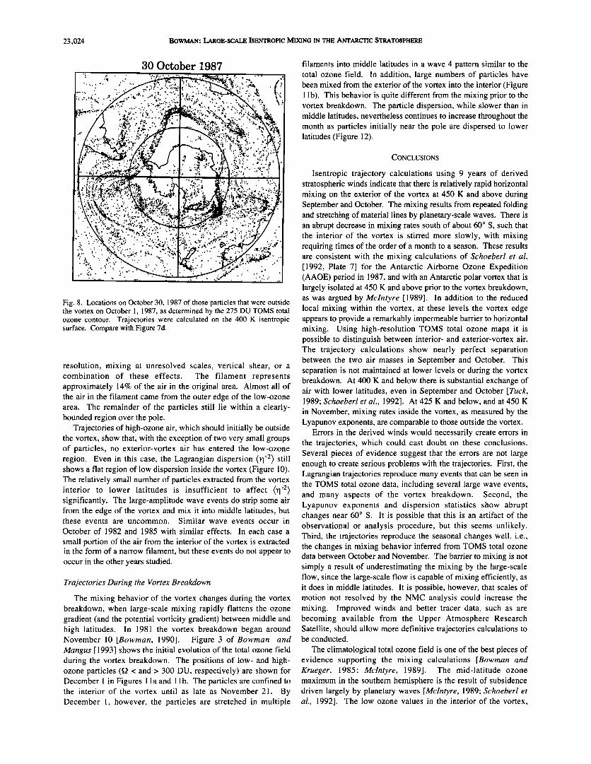
Bowman and Mangus [ 1993, Figure 1 ] presented an example of a large wave event, visible in TOMS total ozone data, that appears to extract a filament of low ozone air from the interior of the vortex. This event occurred between October 19 and 25, 1983. To illustrate the ability of the trajectory calculations to reproduce the general character of this event, trajectories on the 450 K isentropic surface are shown for this period plotted on top of the TOMS total ozone. The TOMS observations are asynoptic, and features can move significant distances in I day, so perfect correspondence between ozone features and trajectories is not to be expected. The locations of particles with total ozone values less than 275 Dobson units (DU) on October 1 are shown on October 21, 23, 25, and 31 in Figure 9. The particles are initially located in a relatively compact and symmetric blob south of 60 ø S (not shown). The blob remains compact through the first half of the month. By October 21 (Figure 9a), however, a large tongue of particles extends toward 135 ø W overlying the low ozone region. During the following 4 days (Figures 9b and 9c) the tongue is stretched into a narrow filament and some particles are pulled into mid-latitude air outside the vortex. The filament of particles closely corresponds to the narrow filament of low total ozone seen by TOMS. The remnants of this filament can still be seen on October 31 (Figure 9d). By this time, the low-ozone filament is no longer visible in the TOMS observations. This could be a result of being stretched to dimensions less than the TOMS

BOWMAN: LARGE-SCALE ISENTROPIC MIXING IN THE ANTARCTIC STRATOSPHERE 23,023

a) I October 1987 b) 30 October 1987

c) I October 1987 d) 30 October 1987

Fig. 7. (a, c) Locations of interior and exterior vortex particles on October 1, 1987, as determined by the 250 DU TOMS total ozone contour. (b, d) Locations of the same groups of particles on October 30, 1987. Trajectories were calculated on the 450 K isentropic surface.

23,024 BOWMAN: LARGE-SCALE ISENTROPIC MIXING IN THE ANTARCTIC STRATOSPHERE

30 October 1987 -.

": .:..-.:?:5! ::-;.

Fig. 8. Locations on October 30, 1987 of those particles that were outside the vortex on October 1, 1987, as determined by the 275 DU TOMS total ozone contour. Trajectories were calculated on the 400 K isentropic surface. Compare with Figure 7d.

resolution, mixing at unresolved scales, vertical shear, or a combination of these effects. The filament represents approximately 14% of the air in the original area. Almost all of the air in the filament came from the outer edge of the low-ozone area. The remainder of the particles still lie within a clearly- bounded region over the pole.

Trajectories of high-ozone air, which should initially be outside the vortex, show that, with the exception of two very small groups of particles, no exterior-vortex air has entered the low-ozone region. Even in this case, the Lagrangian dispersion {rl'2• still shows a flat region of low dispersion inside the vortex (Figure 10). The relatively small number of particles extracted from the vortex interior to lower latitudes is insufficient to affect {rl'2• significantly. The large-amplitude wave events do strip some air from the edge of the vortex and mix it into middle latitudes, but these events are uncommon. Similar wave events occur in

October of 1982 and 1985 with similar effects. In each case a

small portion of the air from the interior of the vortex is extracted in the form of a narrow filament, but these events do not appear to occur in the other years studied.

Trajectories During the Vortex Breakdown

The mixing behavior of the vortex changes during the vortex breakdown, when large-scale mixing rapidly flattens the ozone gradient (and the potential vorticity gradient) between middle and high latitudes. In 1981 the vortex breakdown began around November 10 [Bowman, 1990]. Figure 3 of Bowman and Mangus [1993] shows the initial evolution of the total ozone field during the vortex breakdown. The positions of low- and high- ozone particles (f• < and > 300 DU, respectively) are shown for December 1 in Figures 1 l a and 1 lb. The particles are confined to the interior of the vortex until as late as November 21. By December 1, however, the particles are stretched in multiple

filaments into middle latitudes in a wave 4 pattern similar to the total ozone field. In addition, large numbers of particles have been mixed from the exterior of the vortex into the interior (Figure 1 lb). This behavior is quite different from the mixing prior to the vortex breakdown. The particle dispersion, while slower than in middle latitudes, nevertheless continues to increase throughout the month as particles initially near the pole are dispersed to lower latitudes (Figure 12).

CONCLUSIONS

Isentropic trajectory calculations using 9 years of derived stratospheric winds indicate that there is relatively rapid horizontal mixing on the exterior of the vortex at 450 K and above during September and October. The mixing results from repeated folding and stretching of material lines by planetary-scale waves. There is an abrupt decrease in mixing rates south of about 60 ø S, such that the interior of the vortex is stirred more slowly, with mixing requiring times of the order of a month to a season. These results are consistent with the mixing calculations of Schoeberl et al. [1992, Plate 7] for the Antarctic Airborne Ozone Expedition (AAOE) period in 1987, and with an Antarctic polar vortex that is largely isolated at 450 K and above prior to the vortex breakdown, as was argued by Mcintyre [1989]. In addition to the reduced local mixing within the vortex, at these levels the vortex edge appears to provide a remarkably impermeable barrier to horizontal mixing. Using high-resolution TOMS total ozone maps it is possible to distinguish between interior- and exterior-vortex air. The trajectory calculations show nearly perfect separation between the two air masses in September and October. This separation is not maintained at lower levels or during the vortex breakdown. At 400 K and below there is substantial exchange of air with lower latitudes, even in September and October [Tuck, 1989; Schoeberl et al., 1992]. At 425 K and below, and at 450 K in November, mixing rates inside the vortex, as measured by the Lyapunov exponents, are comparable to those outside the vortex.

Errors in the derived winds would necessarily create errors in the trajectories, which could cast doubt on these conclusions. Several pieces of evidence suggest that the errors are not large enough to create serious problems with the trajectories. First, the Lagrangian trajectories reproduce many events that can be seen in the TOMS total ozone data, including several large wave events, and many aspects of the vortex breakdown. Second, the Lyapunov exponents and dispersion statistics show abrupt changes near 60 ø S. It is possible that this is an artifact of the observational or analysis procedure, but this seems unlikely. Third, the trajectories reproduce the seasonal changes well, i.e., the changes in mixing behavior inferred from TOMS total ozone data between October and November. The barrier to mixing is not simply a result of underestimating the mixing by the large-scale flow, since the large-scale flow is capable of mixing efficiently, as it does in middle latitudes. It is possible, however, that scales of motion not resolved by the NMC analysis could increase the mixing. Improved winds and better tracer data, such as are becoming available from the Upper Atmosphere Research Satellite, should allow more definitive trajectories calculations to be conducted.

The climatological total ozone field is one of the best pieces of evidence supporting the mixing calculations [Bowman and Krueger, 1985; Mcintyre, 1989]. The mid-latitude ozone maximum in the southern hemisphere is the result of subsidence driven largely by planetary waves [Mcintyre, 1989; Schoeberl et al., 1992]. The low ozone values in the interior of the vortex,

BOWMAN: LARGE-SCALE ISENTROPIC MIXING IN THE ANTARCTIC STRATOSPHERE 23,025

a) 21 October 1983 b) 23 October 1983

c) 25 October 1983 d) 31 October 1983

Fig. 9. Locations on October 21, 23, 25, and 31 of those particles that were inside the vortex on October 1, 1983 (f2 < 275 DU). Trajectories were calculated on the 450 K isentropic surface. Particle locations are superimposed on TOMS total ozone for each day.

23,026 BOWMAN: LARGE-SCALE ISENTROPIC MIXING IN THE ANTARCTIC STRATOSPHERE

0 oø

bo o

$0 oø

bo o

O0 ø

• bo o

•0 ø

O0 ø

• bo o

•0 ø

Fig. 10. Particle dispersion (•1'2) for particles on the 450 K isentropic surface during October 1983.

oo o

Fig. 12. Particle dispersion GI'2> for particles on the 450 K isentropic surface during November 1981

a) I December 1981 b) I December 1981

Fig. 11. Locations of interior and exterior vortex particles (as determined from the 300 DU TOMS total ozone contour on November 1, 1981) on December 1, 1981. Trajectories were calculated on the 450 K isentropic surface. Particle locations are superimposed on TOMS total ozone for each day.

I]OWMAN: LARGE-SCALE ISENTROPIC MIXING IN THE ANTARCTIC STRATOSPHERE 23,027

even accounting for the chemical destruction in the ozone hole, strongly suggest that the waves do not penetrate into the interior of the vortex. This evidence supports the hypothesis that the Antarctic vortex provides a good containment vessel for ozone destruction chemistry in the austral spring. Studies of mixing in the wintertime Arctic polar vortex are currently underway, as are plans to examine mixing in the Antarctic during the summer season, when medium-scale waves tend to dominate the circulation.

Acknowledgment,'. My thanks to W.Randel for allowing me to use his compilation of the NMC stratospheric analyses and his codes for the balanced wind calculations. S. Hollandsworth

assisted with the data handling, and S. Dahlberg assisted with the dynamical calculations. The TOMS data were provided on CD- ROM by the National Space Science Data Center at NASA Goddard Space Flight Center. The project scientists for the TOMS instrument are R. McPeters and A. Krueger. This work was funded by NASA Grant NAGW-992 to the University of Illinois at Urbana-Champaign. M. Schoeberl and W. Robinson provided helpful comments on the manuscript.

REFERENCES

Andrews, D. G., J. R. Holton, and C. B. Leovy, Middle Atmosphere Dynamics, pp. 354-361, Academic, San Diego, Calif. 1987.

Bowman, K. P., Evolution of the total ozone field during the breakdown of the Antarctic circumpolar vortex, J. Geophys. Res., 95, 16,529-16,543, 1990.

Bowman, K. P., Barotropic simulation of large-scale mixing in the Antarctic polar vortex, J. Atmos. Sci., 50, 2901-2914, 1993.

Bowman, K. P., and A. J. Krueger, A global climatology of total ozone from the Nimbus-7 Total Ozone Mapping Spectrometer, J. Geophys. Res., 90, 7967-7976, 1985.

Bowman, K. P., and N.J. Mangus, Observations of deformation and mixing of the total ozone field in the Antarctic polar vortex, J. Atmos. Sci., 50, 2915-2921, 1993.

Hartmann, D. L., L. E. Heidt, M. Loewenstein, J. R. Podolske, J.

Vedder, W. L. Starr, and S. E. Strahan, Transport into the south polar vortex in early spring, J. Geophys. Res., 94, 16,779-16,795, 1989.

Kida, H., General circulation of air parcels and transport characteristics derived from a hemispheric GCM, 2, Very long term motions of air parcels in the troposphere and stratosphere, J. Meteorol. Soc. Jpn., 61, 510-523, 1983.

Mcintyre, M. E., On the Antarctic ozone hole, J. Atmos. Terr. Phys., 51, 29-43, 1989.

Mcintyre, M. E., and T. N. Palmer, Breaking planetary waves in the stratosphere, Nature, 305, 593-600, 1983.

McKenna, D. S., R. L. Jones, J. Austin, E. V. Browell, M.P.

McCormick, A. J. Krueger, and A. F. Tuck, Diagnostic studies of the Antarctic vortex during the 1987 Airborne Antarctic Ozone Experiment: Ozone miniholes, J. Geophys. Res., 94, 11,641-11,668, 1989.

Ottino, J. M., The Kinematics of Mixing: Stretching, Chaos and Transport, 364 pp., Cambridge University Press, New York, 1989.

Pierrehumbert, R. T., Chaotic mixing of tracer and vorticity by modulated travelling Rossby waves, Geophys. Astrophys. Fluid Dyn., 58, 285-319, 1991 a.

Pierrehumbert, R. T., Large-scale horizontal mixing in planetary atmospheres, Phys. Fluid,' A, 3, 1250-1260, 1991 b.

Pierrehumbert, R. T., and H. Yang, Global chaotic mixing on isentropic surfaces, J. Atmos. Sci., 50, 2462-2480, 1993.

Plumb, R. A., and J. D. Mahlman, The zonally-averaged transport characteristics of the GFDL general circulation/transport model, J. Atmos. Sci., 44, 298-327, 1987.

Podolske, J. R., M. Loewenstein, S. E. Strahan, and K. R. Chan,

Stratospheric nitrous oxide distribution in the southern hemisphere, J. Geophys. Res., 94, 16,767-16,772, 1989.

Proffitt, M. H., K. K. Kelly, J. A. Powell, B. L. Gary, M. Loewenstein, J. R. Podolske, S. E. Strahan, and K. R. Chan,

Evidence for diabatic cooling and poleward transport within and around the 1987 Antarctic ozone hole, J. Geophys. Res., 94, 16,797-16,813, 1989.

Proflirt, M. H., J. J. Margitan, K. K. Kelly, M. Loewenstein, J. R. Podolske, and K. R. Chan, Ozone loss in the Arctic polar vortex inferred from high-altitude aircraft measurements, Nature, 347, 31-36, 1992.

Randel, W. J., Global Atmospheric Circulation Statistics, 1000- 1 mb, Tech. Note 295+STR, 245 pp., Natl. Cent. for Atmos. Res., Boulder, Colo., 1987.

Randel, W. J., and I. M. Held, Phase speed spectra of transient eddy fluxes and critical layer absorption, J. Atmo,'. Sci., 48, 688-697, 1991.

Rosenfield, J. E., Radiative effects of polar stratospheric clouds during the Airborne Antarctic Ozone Experiment and the Airborne Arctic Stratospheric Expedition, J. Geophys. Res.. 97, 7841-7858, 1992.

Schoeberl, M. R., et al., Reconstruction of the constituent distribution and trends in the Antarctic polar vortex from ER-2 flight observations, J. Geophys. Res., 94, 16,815-16,845. 1989.

Schoeberl, M. R., L. R. Lair, P. A. Newman, J. E. Rosenfield, The

structure of the polar vortex, J. Geophys. Res., 97, 7859-7882, 1992.

Trenberth, K. E., and J. G. Olson, Evaluation of NMC global analyses: 1979-1987, NCAR Tech. Note NCAR/TN-229/+STR, 82 pp. Natl. Cent. for Atmos. Res., Boulder, Colo., 1987.

Tuck, A. F., Synoptic and chemical evolution of the Antarctic vortex in late winter and early spring, 1987, J. Geophys. Res., 94, 11,687-11,737, 1989.

K. P. Bowman, Climate System Research Program, Department of Meteorology, Texas A&M University, College Station, TX 77843-3150.

(Received March 29, 1993; revised August 27, 1993;

accepted August 27, 1993.)