Large Torsional Oscillations in Suspension Bridges Revisited: Fixing an Old ApproximationAuthor(s): P. J. McKennaSource: The American Mathematical Monthly, Vol. 106, No. 1 (Jan., 1999), pp. 1-18Published by: Mathematical Association of AmericaStable URL: http://www.jstor.org/stable/2589581 .Accessed: 16/08/2011 10:07

Your use of the JSTOR archive indicates your acceptance of the Terms & Conditions of Use, available at .http://www.jstor.org/page/info/about/policies/terms.jsp

JSTOR is a not-for-profit service that helps scholars, researchers, and students discover, use, and build upon a wide range ofcontent in a trusted digital archive. We use information technology and tools to increase productivity and facilitate new formsof scholarship. For more information about JSTOR, please contact support@jstor.org.

Mathematical Association of America is collaborating with JSTOR to digitize, preserve and extend access toThe American Mathematical Monthly.

http://www.jstor.org

Large Torsional Oscillations in Suspension Bridges Revisited: Fixing an Old Approximation

P. J. McKenna

1. INTRODUCTION. In Inventions and Technology, Frederic D. Schwartz writes "The Tacoma Narrows Bridge collapse is technology's version of the JFK assassi- nation. There's the grainy black-and-white film endlessly scrutinized frame by frame; the reams of expert analysis next to impossible for a layperson to evaluate; and, of course, the buffs who are convinced that only they know the real story" [29].

He was referring to a "genteel professorial catfight" [28] between some engi- neering writers and me about the explanation of the famous destructive large amplitude torsional oscillation captured on film on November 7th, 1940, and now a staple in physics classes.

Until the collapse of the Tacoma Narrows bridge, it seems that most suspension bridge building had been largely by rule of thumb, without a theoretical underpin- ning. As a result, early bridges, including the Golden Gate bridge and the Tacoma Narrows bridge, exhibited interesting behaviour:

1. they were prone to large-scale oscillation, both torsional and purely vertical 2. occurrence of this large-scale oscillation is dependent on initial conditions

and can be started by a single gust [25] 3. large vertical oscillations could rapidly change, virtually instantaneously, to

torsional oscillation 4. these bridges exhibit localised travelling wave solutions 5. for small oscillation, the observed behaviour is almost perfectly linear.

Good historical sources for these behaviours are [2] and [5]. Of course, these behaviours strongly suggest nonlinearity, and in the late

eighties, following recent and rapid progress in nonlinear analysis of boundary value problems that had just been taking place, I and co-workers attempted to give a mathematical explanation for these phenomena [13], [16-19]. Our starting point was that an unloaded cable cannot be described by the usual Hooke's law, since it resists expansion but not compression. Thus if an unloaded cable is expanded downward by a distance u from the unloaded state, the cable should have a resisting force ku+, in other words, ku if u is positive, and 0 if u is negative. When the cable is loaded, it stretches to a new equilibrium, around which it obeys the linear Hooke's law until deviations from equilibrium become large enough to result in loss of tension when the cable approaches the unloaded state.

Using the tools of nonlinear analysis and numerical investigations, we showed that an equation for a nonlinearly supported beam with this type of nonlinearity could explain both large amplitude vertical periodic oscillations and the travelling wave behaviour. With the usual fervor of the newly converted, I suggested that the

1999] LARGE TORSIONAL OSCILLATIONS 1

nonlinearity induced by the alternate slackening and tightening of the cables could also explain the more famous large amplitude torsional oscillations.

The purpose of this paper is to explore a startling and different possibility. If one is interested solely in a simple version of the Tacoma Narrows oscillation, namely large amplitude torsional oscillation about equilibrium, then the puzzle may have its roots in a simple trigonometry approximation introduced in the engineering literature fifty years ago [5], and unwittingly reproduced ever since, for example in [1].

After the collapse, the initial response of the engineering community, which has served well over the years, was to develop a theory of small oscillations and to construct bridges so that the oscillations stayed in that range. This theory involved many linearising approximations.

The theory was successful in the practical sense. Newer bridges no longer engaged in interesting large amplitude behaviour. And older ones like the Golden Gate were soon modified so that they didn't either.

Of course, when one makes the small angle and other near-equilibrium assump- tions, a theory emerges that cannot explain the large-amplitude motions. Re- designing the bridge to remove the offending behaviour is not the same as mathematically understanding its cause.

This is what the distinguished civil engineering writer, the late Mario Salvadori, meant when he wrote to me " . . . having found obvious and effective physical ways of avoiding the problem, engineers will not give too much attention to the mathematical solution of this fascinating puzzle and [I] am delighted to learn that mathematicians like you are interested in it" [22].

In this paper, we re-derive a mechanical model for a beam or plate oscillating torsionally about equilibrium, and suspended at both sides or ends by cables. We show how the 'small-angle' linearisations can remove a large class of large-ampli- tude nonlinear solutions that can be sustained by extremely small periodic forcing terms.

Based on the original report of the Tacoma Narrows disaster [2], we choose appropriate values for the physical constants in the system of differential equa- tions.

Then we explore the implications and consequences of making, or not making, the trigonometry approximation, and show that even if no loss of tension in the cables is assumed, the nonlinearities introduced by the geometry of the situation are sufficient to explain the large amplitude oscillations seen before the collapse. The large amplitude oscillations that can result from small forcing terms exist over the right range of frequency and amplitude to match the historical observations.

The last nonlinear effect that we listed and would like to explain is the virtually instantaneous change from vertical to torsional oscillation. In Section 4, we explore some of the consequences of assuming that the cables briefly lose tension in a transient way. We observe numerically that when purely vertical oscillations are large enough to allow the supporting cables to lose tension, and the system is subjected to tiny torsional perturbations, the system becomes violently unstable in the torsional dimension.

2. SETTING UP THE MODEL. There is nothing controversial in this section. We set up the equations for vertical and torsional motion of a rod, (or plate), suspended by springs at both ends, (or sides), and free to move vertically and rotate about its center of gravity. In the first subsection, we derive the equations

2 LARGE TORSIONAL OSCILLATIONS [January

from the geometry of the situation, and in the second, we choose reasonable values for the physical constants and the forcing terms.

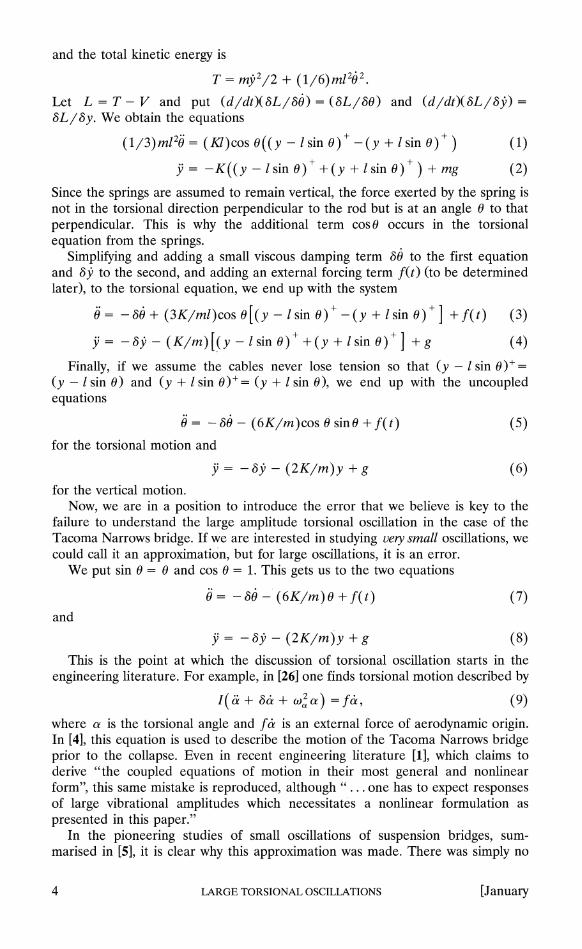
2.1 The equations for vertical and torsional oscillations. If a spring with spring constant K is extended by a distance y, the potential energy is Ky2/2. If a rod of mass m and length 21 rotates about its center of gravity with angular velocity 0, then, its kinetic energy is given by (1/6)ml2(0)2 [31, p. 202]. Assume the rod is suspended as in Figure 1 by springs that resist expansion with a spring constant K at each end. Let y denote the downward distance of the center of gravity of the rod from the unloaded state. Let 0 denote the angle of the rod from the horizontal. Let y be the positive part of y, that is, y+ = max {y, 0}.

nonlinear cable-like springs

The vertical deflection of the center of

the deflection from horizontal

Figure 1. A cross-section of the bridge as an inflexible rod supported by two springs at each side, giving rise to the system of equations (3) and (4) and simplifying to (5) and (6) when there is no loss of tension.

The potential energy due to gravity is - mgy. The extension is (y - l sin 0) + in one spring and (y + l sin 0 ) in the other. Actually, this involves another hidden small-angle assumption, namely that the cables remain vertical, although the lateral motion of the ends of the plate or rod deflects them slightly to the left or right. Thus, this model actually overstates slightly the resistance to torsional motion. When the cables are of length 100 feet and the lateral motion is about six feet, as they were in the Tacoma Narrows bridge, this seems a reasonable approximation.

Thus, the total potential energy is

V= (K/2)(((y - lsin 0) )2 + (y + lsin 0) ) - mgy

1999] LARGE TORSIONAL OSCILLATIONS 3

and the total kinetic energy is

T = my 2/2 + (1/6)ml26 2.

Let L = T - V and put (d/dt)(8L/80) = (8L/80) and (d/dt)(8L/8j) =

8L/8y. We obtain the equations

(1/3)m126 = (Kl)cos 0((y - lsin 0) -(y + lsin 0) ) (1)

j = -K((y - lsin 0)+ +(y + lsin 0) ) + mg (2) Since the springs are assumed to remain vertical, the force exerted by the spring is not in the torsional direction perpendicular to the rod but is at an angle 0 to that perpendicular. This is why the additional term cos 0 occurs in the torsional equation from the springs.

Simplifying and adding a small viscous damping term 80 to the first equation and 8b to the second, and adding an external forcing term f(t) (to be determined later), to the torsional equation, we end up with the system

0 = - 80 + (3K/ml)cos 0[(y - I sin 0) - (y + I sin 0) ] + f(t) (3)

8 -b - ( Klm) [( y - I sin 0 ) + +( y + I sin 0 ) ] + g (4) Finally, if we assume the cables never lose tension so that (y - 1 sin 0)+-

(y - lsin 0) and (y + lsin 0)+= (y + lsin 0), we end up with the uncoupled equations

0 = -80 - (6K/m)cos 0 sine + f(t) (5)

for the torsional motion and

y = - 8b - (2K/m)y + g (6)

for the vertical motion. Now, we are in a position to introduce the error that we believe is key to the

failure to understand the large amplitude torsional oscillation in the case of the Tacoma Narrows bridge. If we are interested in studying very small oscillations, we could call it an approximation, but for large oscillations, it is an error.

We put sin 0 = 0 and cos 0 = 1. This gets us to the two equations

0 = -860 - (6K/m) 0 + f (t) (7) and

j =-_ 685 - (2K/m)y + g (8)

This is the point at which the discussion of torsional oscillation starts in the engineering literature. For example, in [26] one finds torsional motion described by

I(r+ Nor + (o 2 a) = 6i a ~~~~~~~~~(9) where a is the torsional angle and f6i is an external force of aerodynamic origin. In [4], this equation is used to describe the motion of the Tacoma Narrows bridge prior to the collapse. Even in recent engineering literature [1], which claims to derive "the coupled equations of motion in their most general and nonlinear form", this same mistake is reproduced, although ... . one has to expect responses of large vibrational amplitudes which necessitates a nonlinear formulation as presented in this paper."

In the pioneering studies of small oscillations of suspension bridges, sum- marised in [5], it is clear why this approximation was made. There was simply no

4 LARGE TORSIONAL OSCILLATIONS [January

technology available to solve nonlinear equations like (5). There was no choice but to linearize the equation and hope the errors introduced were not too big. Indeed, experience showed that for very small oscillations, this was reasonable.

However, today we can solve (5) accurately. Thus we can determine whether there is an important difference between the trigonometrically correct model and the linear one. But before we do this, we should choose appropriate constants. This is the task of the next subsection.

2.2 Choosing physical constants and external forcing term. Our main source is [2]. Since the model is very simple, we do not concern ourselves with very precise choice of constants but content ourselves with getting the magnitudes about right. The mass of a foot of the bridge was about 5,000 lbs. so we choose the m in our equations to be 2,500 kgs. The width of the bridge was about 12 meters so we choose 1 to be 6.

The bridge would deflect about .5 meters when loaded with 100 kgs. for each .3 m. of bridge. Since there are two springs, this gives the equation 2K(.5)= 100(9.8) for 2Ky = mg, and we choose K = 1000.

For the external forcing term, we choose f(t) = A sin at and investigate the response of the different equations to this type of periodic forcing. The frequency of the motion of the bridge before the collapse was about 12 to 14 cycles per minute so we take ,u between 1.2 to 1.6.

There does not seem to be much information about the amplitude of the forcing term, although there was an attempt to measure it in [26]. Apparently, one can measure small oscillations caused by forces that induce oscillations of about 3 deg. "It was found necessary to permit only small amplitudes of oscillation to occur, (e.g. in torsion 0 < a < ? 3 deg)" [sic]. Thus, we choose A small enough to create oscillation of this order of magnitude in the linear model.

Finally, there is a consensus that the term describing the viscous damping should have a coefficient of about .01 [2].

We now have a system that, in the absence of forcing, settles down to an equilibrium with y = 12.25 and 0 = 0. As long as the oscillation is such that the y + 1 sin 0 remains below zero, i.e., the deflections upward from equilibrium do not exceed about 12 meters, the equations remain uncoupled, and we investigate the long-term behaviour of the forced pendulum equation (5) versus the linearized version (7) with these constants and a variety of initial conditions and small forcing terms,

2.3 What happened at Tacoma Narrows. We recall what happened before the collapse. Again, our source is [2].

The bridge engaged in vertical oscillations even during construction. "Prior to 10.00 A.M. on the day of the failure, there were no recorded instances of the oscillation being otherwise than with the two cables in phase and with no torsional motion."

On November 7, for some time before 10:00 AM, the bridge was engaged in what seemed like normal vertical motions, with amplitudes of about 5 feet and a frequency of about 38 per minute. The motion was apparently more violent than usual, with eight nodes. Then the torsional motion began, as the bridge was being observed by Professor F. B. Farquharson [2]:

... a violent change in the motion was noted. This change appeared to take place without any intermediate stages and with such extreme violence that the span appeared to be about to roll completely over.

1999] LARGE TORSIONAL OSCILLATIONS 5

The motion, which a moment before had involved a number of waves, (nine or ten) [This means a eight-or-nine noded vertical motion], had shifted almost instantly [our emphasis] to two [a one-noded torsional motion]. At the moment of first observing the main span,..., the motion had a frequency of 14 cycles per minute. ... the node was at the center of the main span and the structure was subjected to a violent torsional action about this point. At times, for a short period, the motion changed over to a single wave on each cable but still with the cables out of step. This motion, which never lasted long seemed to be of slightly greater amplitude than the single-noded motion, but of the same frequency. [This motion, of double amplitude of 28 feet continued for approximately forty-five minutes.]

There is no consensus on what caused the sudden change to torsional motion. In [23, p. 209], this transition is explained as "some fortuitous condition broke the bridge action."

It may have been a minor structural failure, enough to jar the bridge in a torsional direction. We explore the consequences of just such a single push on the two models we compare: the linear and the trigonometric ones. Thus, it is our task to look for large-amplitude periodic motions that are primarily torsional with an amplitude of about + 1 radian, corresponding to a small torsional forcing term with a frequency in the neighbourhood of 12 to 14 cycles per minute.

2.4 A few words about forcing. We have to choose some method to model the aerodynamic and other forces acting on the bridge that cause it to go into a periodic motion. There is really no way to say precisely what the forces would be when a huge structure is oscillating up and down by 28 feet every five seconds.

According to [26], for a cross-section similar to the Tacoma Narrows bridge in a wind tunnel, the aerodynamic forces induced approximately sinusoidal oscillations of amplitude of plus or minus three degrees. In all our experiments, we explore the response of the system to a sinusoidal forcing term of the form A sin ( ,u t). We then choose the value of A in order to induce oscillations of three degrees near equilibrium in the linear model.

In this sense, we have chosen the particular form Asin ( ,uat) as a 'generic' oscillatory force, with the right frequency and amplitude. The conclusions would be the same for any other oscillatory force of roughly the same magnitude and frequency. For example, we repeated some of these experiments for the forcing term A(sin ( utt))3. The results were qualitatively the same: small forcing could give rise to either large or small periodic long-term behaviour, with the eventual outcome dependent on the initial conditions.

3. NUMERICAL EXPERIMENTS: THE EFFECT OF NOT LINEARIZING. We now investigate the response of the two equations to various initial conditions and forcing terms. Our first equation, with the correct trigonometry is

0 = -0.01 0 - (2.4) cos Osin 0 + A sin ,utt, (10)

which when linearized becomes

6 LG T0.01 N - O(2.4)L0 + ATsin [ rt. (11)

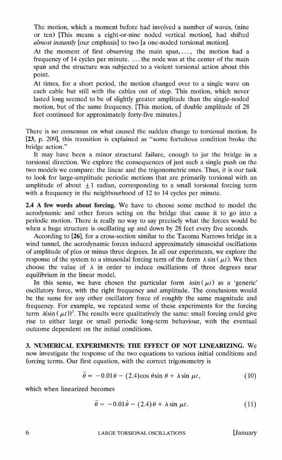
3.1 Long-term behaviour with and without The Error. We start with initial condi- tions that mimic a large torsional push. We choose 0(0) = 1.2 and 0(0) = 0, and start with ,u = 1.2 and A = 0.06. We run the initial value problem for one thousand periods to see what the system has settled down to. This is shown in Figure 2.

s 0.5-

0;

T 10.5

0 0.1 002 0.3 0.4 0.5 0.6 0.9 1 The last 16 of 1000 periods of the forcing temn

CO 0

0 -0

0 0.1 0.2 0.3 0.4 0.5 0.6 0.7 0.8 0.9 1 The last 16 of 1000 periods of the forcing term

Figure 2. The difference in long-term outcomes depending on whether we solve the trigonometrically correct equation (10) or the linearized equation (11) with a large torsional push and a small periodic forcing term.

On the top of Figure 2, the linear oscillator has settled to an oscillation of approximately ?3 deg. Since this is true of all experiments we run, we do not repeat the picture, but simply remark that in the linear oscillator, the oscillation has died off.

The bottom half of Figure 2 shows that the torsional oscillator of equation (10) has settled into a periodic oscillation of large amplitude. The single large push at the start of the experiment has induced a permanent large amplitude torsional oscillation. This solution represents a torsional oscillation of about one radian, with a period of about 5.2, and a vertical amplitude at the sides of about the correct amount of 10 meters. The period is a little larger than the range of 4.25-5.00 reported in the bridge, but it is certainly a reasonable approximation.

Now we solve the initial value problem for the trigonometric oscillator with the initial conditions 6(k) = 0 and 6(k) = 0. This time, it eventually settles down to the small periodic oscillation shown in Figure 2. The results of solving the trigonometric oscillator for large and small torsional pushes is contrasted in Figure 3. If the initial values remain small, one can end up in what is basically the linear situation: compare the top graphs in Figures 2 and 3. On the other hand, the large torsional push can result in the large amplitude oscillation shown in the bottom graphs of Figures 2 and 3.

This is the phenomenon that we wish to emphasize: the trigonometric oscillator can have several different periodic responses to the same periodic forcing term. Which

1999] LARGE TORSIONAiL OSCILLATIONS 7

0.5

0

- 0.5

-10 0.1 0.2 0.3 0.4 0.5 0.6 0.7 0.8 0.9 1

0 - 0.5-

0 0.1 0.2 0.3 0.4 0.5 0.6 0.7 0.8 0.9 1

Figure 3. Eventual behaviour of the trigonometrically correct oscillator combining a large torsional push (bottom) or small (top), both with a small torsional forcing term with ,u at 1.2.

response eventually results can be determined by a simple transient event such as a large single push.

Let's explore this a little more. We take ,u = 1.3. Also, take A = 0.02, enough to induce an oscillation in the linear oscillator of + 1 deg. Needless to say, even after the large push, the linear oscillator settles down after a large time to near-equilibrium, as seen in Figure 4. Here, the period, matching that of the forcing term, is a more realistic 4.83. Again, the large push induces a permanent large torsional oscillation in the trigonometric oscillator, of slightly smaller ampli- tude than the earlier case, but still huge.

The same results occur if we take A = 1.4, where we get a large amplitude oscillation with a period of 4.5, corresponding closely to that reported (about 4.3) at the start of the torsional oscillation on the bridge. Later, it seems to have slowed down to 5.0.

Similar results were obtained for ,u= 1.5 but they disappear above this value until one approaches values of ,u that are integer multiples of the values we have been discussing. At these values subharmonic behaviour occurs, as we discuss in Section 3.2.

-1

0.5

- 0.5

-1 l l l l l l l l l

0 0.1 0.2 0.3 0.4 0.5 0.6 0.7 0.8 0.9 1

0.5

0 - 0.5

0 0. 1 0. 2 0.3 0.4 0.5 0.6 0.7 0.8 0.9 1

Figure 4. Multiple periodic solutions similar to Figure 3, but with ,u changed to 1.3.

8 LARGE TORSIONAL OSCILLATIONS [January

1

0.5;

0 - 0.5-

-1 0 0.1 0.2 0.3 0.4 0.5 0.6 0.7 0.8 0.9 1

0.5

0

- 0.5

-1 l l l l l l l l l 0 0.1 0.2 0.3 0.4 0.5 0.6 0.7 0.8 0.9 1

Figure 5. Multiple periodic solutions similar to Figure 3, but with ,u changed to 1.4.

This is the most important conclusion of this article: over a range of frequency that is close to that observed before the collapse of the Tacoma Narrows, the final oscillation that results in, the trigonometric oscillator after a large time can be either small or very large. All it may take is a single push to change the eventual outcome from small near-equilibrium behaviour to large torsional periodic mo- tions.

3.2 Subharmonic responses. Anyone familiar with nonlinear dynamics who has read this far doubtless wonders why we are emphasizing responses of the same period as the forcing term. In fact, we expect that the periodic solutions of (10) discussed in the previous section can be sustained, not just by the forcing term of the same period but with one of double or triple the period.

In Figure 6, we show two periodic solutions corresponding to a forcing term A sin ,ut with ,u = 2.6. The solution is similar to that found at ,u = 1.3. The figure looks a little different because the last sixteen periods of the forcing term are shown so the x-scale is half the one shown in Figure 4.

All the remarks of the previous section apply to solutions that are subharmonic responses.

1

0 0.1 0.2 0.3 0.4 0.5 0.6 0.7 0.8 0.9 1

0 -1~~~~~~~~~~~~~~~~~~~~~~~~~~~~.

0 0.1 0.2 0.3 0.4 0.5 0.6 0.7 0.8 0.9 1

Figure 6. A subharmonic response to periodic forcing. Here, with ,u = 2.6, the large and small initial conditions give rise to either a small linear response of the same period or to one of twice the period similar to that seen around ,u = 1.3.

1999] LARGE TORSIONAL OSCILLATIONS 9

The most intriguing values of ,u to investigate may be when it is near 4. This is because the vertical motions that preceded the torsional ones had a frequency (about 40 per minute) that corresponded to approximately this value, strongly suggesting the existence of some forcing term of this frequency.

Sure enough, when the nonlinear system is forced at this frequency, one obtains a periodic response to a large initial condition and a small forcing term of approximately the right frequency and magnitude. This is shown in Figure 7, where a forcing term A sin 4t is taken, and combined with either a large or small initial condition. Varying the initial conditions can result in either small linear responses of the right period (with small initial conditions) or large nonlinear responses similar to those described earlier, with period three times that of the forcing term.

0 0.1 0.2 0.3 0.4 0.5 0.6 0.7 0.8 0.9 1

0

0 0.1 0.2 0.3 0.4 0.5 0.6 0.7 0.8 0.9 1

Figure 7. These torsional oscillations corresponds to large and small initial conditions if u = 4, corresponding to the frequency of the earlier vertical oscillations in the bridge, before the onset of torsional motion.

3.3 Some transient results. Now we illustrate how dramatically different the transient behaviour is for the trigonometrically correct and the linearized system. We solve the initial value problem for a variety of different initial conditions and compare the two systems. Throughout this subsection, where a forcing term has been used, it is of the form A sin (1.2t), although similar results would occur around ,u-= 1.3 or 1.4.

First, the good news. If we solve the initial value problem with no forcing but with large initial

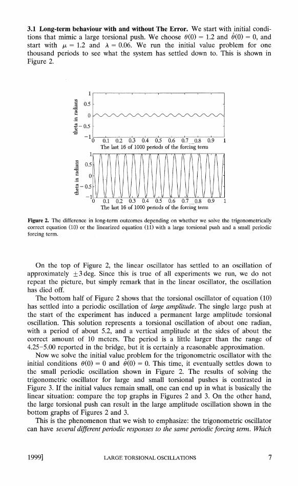
conditions, the results over the first hundred periods for the two problems are shown in Figure 8. There is little real difference, as the damping takes over and both systems settle back to equilibrium.

Now, do the same experiment starting with initial conditions at equilibrium, but with a small forcing term A = 0.05. Again, the two systems give close results. This is shown in Figure 9.

So far, so good! When subjected separately either to small periodic forcing or to a large transient displacement from equilibrium, the system responds with much the same behaviour in the linear and nonlinear models.

Now to the results that we have already discussed. If we combine the previous two effects, the principle of superposition predicts that the linear system will die down as before. Figure 10 shows this, as well as the huge difference caused by doing the correct trigonometry. The trigonometrically correct model continues

10 LARGE TORSIONAL OSCILLATIONS [January

0.5

0

- 0.5

0 0.1 0.2 0.3 0.4 0.5 0.6 0.7 0.8 0.9 1

1 u4

0.5

0.

0 0.1 0.2 0.3 0.4 0.5 0.6 0.7 0.8 0.9 1

Figure 8. The result of a large push from equilibrium, in both the linear and correct models, with no forcing term.

0.2

0.1

0

-021 t v -0.01

* 0 0.1 0.2 0.3 0.4 0.5 0.6 0.7 0.8 0.9 1

u4 0.2 --

iji i#8 -02 - 0 0.1 0.2 0.3 0.4 0.5 0.6 0.7 0.8 0.9 1

Figure 9. The result of a small forcing term starting at equilibrium. Both systems start to die down immediately.

1

-05 _~1 _II

0 0.1 0.2 0.3 0.4 0.5 0.6 0.7 0.8 0.9 1

2 u4

-2 0 0.1 0.2 0.3 0.4 0.5 0.6 0.7 0.8 0.9 1

Figure 10. The transient behaviour resulting from combining the two influences shown separately in Figures 8 and 9. Predictably, the linear model starts to die down but the nonlinear one goes into large oscillation.

1999] LARGE TORSIONAL OSCILLATIONS 1 1

indefinitely in a large torsional oscillation, eventually settling to the large periodic motion introduced in Figure 2.

Finally, we show how sensitive the correct system is to the amplitude of the forcing term. Figure 11 shows the effect of changing the amplitude of the forcing term from A = 0.05 (top), which results in the large amplitude motion, to A = 0.04 (bottom), when the motion begins immediately to die down.

2

-2 O 0.1 0.2 0.3 0.4 0.5 0.6 0.7 0.8 0.9 1

u4

0.

-0.5

0 0.1 0.2 0.3 0.4 0.5 0.6 0.7 0.8 0.9 1

Figure 11. A slight change in the amplitude of the forcing term can make a huge difference in the nonlinear model. The effects of a large push with A = 0.04 and A = 0.05 are compared. The slight increase is enough to change the eventual behaviour from small near-equilibrium motion to large and destructive motion.

3.4 A quick summary. Performing the unnatural act of linearizing the trigonomet- ric oscillator of equation (10) has the effect of removing a large class of large amplitude behaviours.

As shown in Figures 8 and 9, the linear model is good in the presence of a large transient push and no forcing, or if one starts off at equilibrium with small forcing. However, when these two effects are combined, it completely fails to predict the eventual long-term behaviour of the real system (10).

In the trigonometrically correct model, over a wide range of frequency, several different amplitude oscillations can exist for the same periodic forcing term. Which one the system ends up on can depend on simple transient events, such as a single large push. Large amplitude solutions can result as a subharmonic response to a higher frequency forcing term and are of roughly the right magnitude and fre- quency when compared to the oscillation of the Tacoma Narrows bridge in its final torsional oscillations.

We emphasize that there is nothing high-tech or controversial about these results.

It is well known that a periodically forced pendulum equation such as (5) exhibits multiple solution and chaotic behaviour [10]. Perhaps the only surprise is that when one makes reasonable guesses for the constants based on the available literature, the resulting periodic motions are so good a match to the historical data.

One simply recognizes that trigonometry has been artificially removed from the problem, restores it, and uses a good Runge-Kutta initial value solver to find the long-time behaviour of the system.

12 LARGE TORSIONAL OSCILLATIONS [January

There remain two other things to understand: first, what was the origin of the original vertical oscillations of up to 5 ft. in amplitude and with a frequency of about 40 per minute? If we assume these oscillations were approximately sinu- soidal, accelerations must have been approaching that of gravity.

Second, one can ask about the origin of the sudden transition from vertical to torsional motion. On this question, we may need to be more speculative or controversial, as we shall see in the next section. However, as regards the large amplitude torsional periodic solution, we believe the explanation of this section is satisfactory.

4. WHAT IF THE SPRINGS LOSE TENSION BRIEFLY? THE TRANSITION TO TORSIONAL MOTION. So far, we have focussed on the least controversial results: namely, if one does not artificially remove the trigonometry from the torsional oscillator, one gets a realistic explanation for the oscillations seen in the Tacoma Narrows bridge before its collapse. We have largely avoided the question of what happens when the two equations (3) and (4) are coupled due to periodic slackening of the cables.

If this does happen, the structure of the periodic solutions becomes consider- ably more complex. A start to studying this system and hints of the complexities that arise can be found in [12].

There is some controversy about this question. I and co-workers claim that with accelerations reaching that of gravity, and with magnitudes of up to 28 ft. every four seconds, there must have been some slackening of the cables. Some engineers insist, to the verge of apoplexy, that this cannot happen [3]. A third group take a middle path, claiming that the cables can slacken only in a brief and transitory fashion [3].

In this final section, we follow the middle path and ask what happens to the initial value problem solution of the full nonlinear system, if the cables briefly lose tension due to a vertical motion.

Here, we come to a new and unexpected conclusion: a purely vertical nontor- sional motion in which the cables lose tension can become disastrously unstable even in the presence of tiny torsional forces, setting up a rapid transition to large amplitude torsional motion. This might be the explanation for the sudden transition observed at Tacoma Narrows.

We have no good mathematical explanation for this phenomenon. However, we can demonstrate it in a sequence of mathematical experiments.

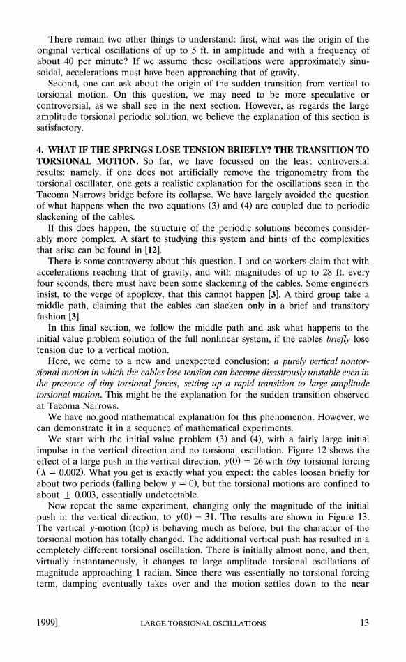
We start with the initial value problem (3) and (4), with a fairly large initial impulse in the vertical direction and no torsional oscillation. Figure 12 shows the effect of a large push in the vertical direction, y(0) = 26 with tiny torsional forcing (A = 0.002). What you get is exactly what you expect: the cables loosen briefly for about two periods (falling below y = 0), but the torsional motions are confined to about + 0.003, essentially undetectable.

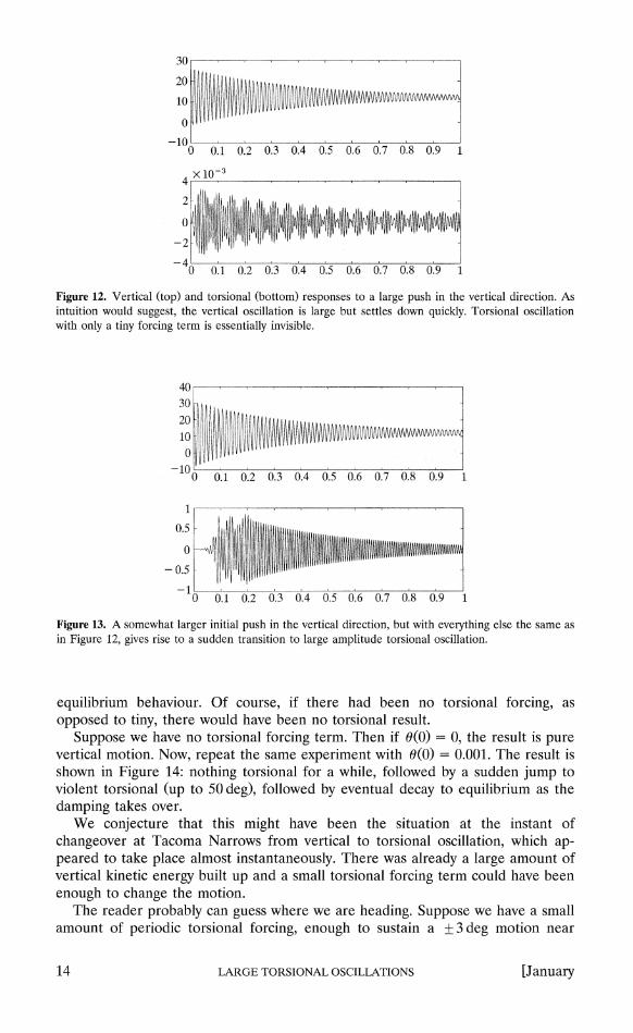
Now repeat the same experiment, changing only the magnitude of the initial push in the vertical direction, to y(0) = 31. The results are shown in Figure 13. The vertical y-motion (top) is behaving much as before, but the character of the torsional motion has totally changed. The additional vertical push has resulted in a completely different torsional oscillation. There is initially almost none, and then, virtually instantaneously, it changes to large amplitude torsional oscillations of magnitude approaching 1 radian. Since there was essentially no torsional forcing term, damping eventually takes over and the motion settles down to the near

1999] LARGE TORSIONAL OSCILLATIONS 13

30

20 : ',

-10

o 01 0.2 0.3 0.4 0.5 0.6 0.7 0.8 0.9 1

X10-3

-4 0 0.1 0.2 0.3 0.4 0.5 0.6 0.7 0.8 0.9 1

Figure 12. Vertical (top) and torsional (bottom) responses to a large push in the vertical direction. As intuition would suggest, the vertical oscillation is large but settles down quickly. Torsional oscillation with only a tiny forcing term is essentially invisible.

40 30 H 20

-10

o 0.1 0.2 0.3 0.4 0.5 0.6 0.7 0.8 0.9 1

-10

0 0.1 0.2 0.3 0.4 0.5 0.6 0.7 0.8 0.9 1

Figure 13. A somewhat larger initial push in the vertical direction, but with everything else the same as in Figure 12, gives rise to a sudden transition to large amplitude torsional oscillation.

equilibrium behaviour. Of course, if there had been no torsional forcing, as opposed to tiny, there would have been no torsional result.

Suppose we have no torsional forcing term. Then if 0(0) = 0, the result is pure vertical motion. Now, repeat the same experiment with 0(0) = 0.001. The result is shown in Figure 14: nothing torsional for a while, followed by a sudden jump to violent torsional (up to 50 deg), followed by eventual decay to equilibrium as the damping takes over.

We conjecture that this might have been the situation at the instant of changeover at Tacoma Narrows from vertical to torsional oscillation, which ap- peared to take place almost instantaneously. There was already a large amount of vertical kinetic energy built up and a small torsional forcing term could have been enough to change the motion.

The reader probably can guess where we are heading. Suppose we have a small amount of periodic torsional forcing, enough to sustain a +3 deg motion near

14 LARGE TORSIONAL OSCILLATIONS [January

40

30;j - 30

-10 0 0.1 0.2 0.3 0.4 0.5 0.6 0.7 0.8 0.9 1

-1-1 -2 , , ,

0 0.1 0.2 0.3 0.4 0.5 0.6 0.7 0.8 0.9 1

Figure 14. No torsional forcing term, but a tiny displacement in the initial value of 6(0) is also enough to induce violent torsional oscillation, which, in the absence of periodic forcing, eventually dies down due to damping.

equilibrium. We have already seen how a single large torsional push could induce a large-amplitude periodic torsional motion. Now we consider the influence of a large vertical push combined with the small amount of periodic torsional forcing. The result is shown is Figure 15.

Here we have taken [t as 1.3, in the middle of the range where we expect multiple solutions. We have taken A = 0.02, about enough to induce linear oscillation of about + 2 deg. We have given a sufficiently large push in the vertical direction to cause the springs to lose tension for the first five cycles. The result is a couple of cycles of small torsion, followed by an almost instantaneous transition to huge torsional motion, which remains permanent. It eventually settles down to the permanent periodic torsional motion shown in Figure 4.

We believe that we have discovered a convincing explanation for the mystery of the sudden transition to torsional motion. A large vertical motion had built up, there

-10

-10 0.1 0.2 0.3 0.4 0.5 0.6 0.7 0.8 0.9 1

1 -0) 0.5

0 - 0.5-

-10 0.1 0.2 0.3 0.4 0.5 0.6 0.7 0.8 0.9 1

Figure 15. What really happened to induce torsional oscillation at Tacoma Narrows? A small but periodic torsional force combines with a large vertical transient push to produce a rapid transition to large torsional oscillation as the vertical oscillation is damped away.

1999] LARGE TORSIONAL OSCILLATIONS 15

was a small push in the torsional direction to break symmetry, the instability occurred, and small aerodynamic torsional periodic forces were sufficient to maintain the large periodic torsional motions, as shown in Figure 15.

5. SOME CONCLUDING COMMENTS. No mathematical model is ever perfect. Turing said it best: "This model will be a simplification and an idealization, and consequently a falsification. It is to be hoped that the features retained for discussion are those of the greatest importance in the present state of knowledge" [32]. Let us review some of the short-comings of our paper.

Following the engineering literature, we have treated the cable-suspension structure as a torsional oscillator supported by springs that remain linear until they reach the unloaded state. We doubt that a bridge oscillating up and down by about 10 meters every 4 seconds obeys Hooke's law.

Our model slightly understates the period of the large amplitude torsional oscillations. This is probably due to the fact that there is additional resistance to torsion from the road-bed, adding an extra spring constant to equation (10).

Our model says very little about the vertical oscillation that preceded the torsional oscillation. It may explain why the vertical motion was so rapidly converted to torsional motion, but has little to say about why this original motion started and continued. Nor does it say much about the rather mysterious complex torsional motion that actually occurred, namely one that alternated between one-noded and no-noded oscillations.

However, it still gives a remarkably "low-tech" explanation of two of the phenomena, the large amplitude torsional motions and the transitional motions.

There remains a great deal to do on the coupled system. With a reliable Runge-Kutta solver and unlimited computer time (and some patience), the reader can discover new phenomena in the solution set of this system. Certainly, this type of experimentation makes for interesting class projects in the undergraduate environment.

A mathematical explanation for the apparently unstable nature of the large amplitude vertical oscillation in which cables lose tension would be desirable. Although large amplitude vertical oscillations have been investigated and their one-dimensional stability proved [13], we have no proof of their instability in the torsional direction. An intuitive argument might be advanced that if the rod is ever in the situation where one spring is under tension and the other is not, this introduces a new large torsional force.

Finally, we are not sure of the consequences of this work for modern suspension bridges in earthquake conditions. Part of the dilemma, as one leading bridge engineer has lamented, is that there is a "lack of open discussion" on these problems [6].

It is not clear whether, in their calculations about earthquake responses, engineers have taken into account the potentially catastrophic consequences of a brief loosening of the cables and the ensuing large amplitude torsional oscillations that can result. To judge by the literature, they are still making the small oscillation linearization, which can be so misleading once away from equilibrium [1]. Since hundreds of millions of dollars are being spent in an effort to strengthen suspension bridges in California in preparation for large earthquakes, this question may not be entirely academic.

Finally, it is worth remarking that our results illustrate how the availability of inexpensive computation is changing the entire culture of mathematics. Now, new

16 LARGE TORSIONAL OSCILLATIONS [January

and interesting results can be discovered in the undergraduate classroom. We can now investigate numerically simple systems such as (4) and (5), and we uncover beautiful new properties that we could not have suspected previously. We may be witnessing the dawn of a new golden age of discovery in nonlinear oscillations.

REFERENCES

1. A. M. Abdel-Ghaffar, Suspension bridge vibration: Continuum formulation, Jour. Eng. Mechanics, A.S.C.E. 108 (1982) 1215-1232.

2. 0. H. Amann, T. von K'arman, and G. B. Woodruff, The Failure of the Tacoma Narrows Bridge, Federal Works Agency, 1941.

3. D. Berreby, The great bridge controversy, Discover 13 (1992) 26-33. 4. K. Y. Billah, and R. H. Scanlan, Resonance, Tacoma Narrows bridge failure, and undergraduate

physics textbooks, Amer. J. Physics 59 (1991) 118-124. 5. F. Bleich, C. B. McCullough, R. Rosecrans, and G. S. Vincent, The Mathematical Theory of

Suspension Bridges. U.S. Dept. of Commerce, Bureau of Public Roads, 1950. 6. A. Castellani, Safety Margins of suspension bridges under seismic conditions, ASCE J. Structural

Engineering 113 (1987) 1600-1616. 7. A. Castellani, and P. A. Felotti, A note on lateral vibration of suspension bridges, ASCE J.

Structural Engineering 112 (1986) 2169-2173. 8. Y. Chen, and P. J. McKenna, Traveling waves in a nonlinearly suspended beam: theoretical results

and numerical observations, J. Differential Equations, 136 (1997) 325-355. 9. Y. S. Choi, K. C. Jen, and P. J. McKenna, The structures of the solution set for periodic

oscillations in a suspension bridge model, IMA J. Appl. Math. 47 (1991) 283-306. 10. P. Blanchard, R. L. Devaney, and G. Hall, Differential Equations, PWS Publishing, Boston, 1996. 11. S. H. Doole, and S. J. Hogan, A piecewise linear suspension bridge model: Nonlinear dynamics

and orbit continuation, Dynamics Stability Systems 11 (1996) 19-47. 12. S. H. Doole, and S. J. Hogan, Torsional dynamics in a simple suspension bridge model, Applied

Nonlinear Mathematics Research Report Number 9.96, University of Bristol, Bristol, 1996. 13. J. Glover, A. C. Lazer, and P. J. McKenna, Existence and stability of large-scale nonlinear

oscillations in suspension bridges, Z. Angew. Math. Phys. 40 (1989) 171-200. 14. D. Jacover and P. J. McKenna, Nonlinear torsional flexings in a periodically forced suspended

beam, J. Comput. Appl. Math. 52 (1994) 241-265. 15. Theodore von Karman, The Wind and Beyond, Theodore von Kdrma'n, Pioneer in Aviation and

Pathfinder in Space, Little Brown and Co. Boston, 1967. 16. A. C. Lazer, and P. J. McKenna, Large amplitude periodic oscillations in suspension bridges: some

new connections with nonlinear analysis, SIAM Review 32 (1990) 537-578. 17. A. C. Lazer, and P. J. McKenna, Large scale oscillatory behaviour in loaded asymmetric systems,

Analyse Nonlineaire Annales de L'Institut Henri Poincare 4 (1987) 243-274. 18. P. J. McKenna, and W. Walter, Nonlinear oscillations in a suspension bridge, Arch. Rat. Mech.

Anal. 98 (1987) 167-177. 19. P. J. McKenna, and W. Walter, Travelling waves in a suspension bridge, SIAM J. Appl. Math. 50

(1990) 703-15. 20. I. Peterson, Rock and Roll Bridge, Science News 137 (1990) 344-346. 21. H. Petroski, Still twisting, American Scientist, September-October, 1991. 22. Mario Salvadori, personal communication. 23. R. H. Scanlan, Developments in low-speed aeroelasticity in the civil engineering field, AL4A

Journal 20 (1982) 839-844. 24. R. H. Scanlan, Airfoil and bridge deck flutter derivatives, Proc. Amer. Soc. Civ. Eng. Eng. Mech.

Division EM6 (1971) 1717-1737. 25. R. H. Scanlan, The action of flexible bridges under wind II: buffeting theory., J. Sound and

Vibrations 60 (1978) 201-211. 26. R. H. Scanlan, and J. J. Tomko, Airfoil and bridge deck flutter derivatives, Proc. Amer. Soc. Civ.

Eng. Eng. Mech. Division EM6 (1971) 1717-1737.

1999] LARGE TORSIONAL OSCILLATIONS 17

27. R. H. Scanlan, and J. W. Vellozi, Catastrophic and annoying responses of long-span bridges to wind action, Annals New York Acad. Sciences 352 (1980) 247-263.

28. F. D. Schwarz, Why theories fall down, American Heritage of Inventions and Technology 8 (1993) 6-7.

29. F. D. Schwarz, Still Falling, American Heritage of Inventions and Technology 9 (1993) 7. 30. Seattle Times/Seattle Post-Intelligencer, November 5, 1990 p. 12. 31. J. L. Synge, and B. A. Griffith, Principles of Mechanics, McGraw-Hill, New York, 1959. 32. A. M. Turing, The chemical basis of morphogenesis, Philos. Trans. Royal Soc. Ser. B 237 (1952)

37-72. 33. P. Vielsack, and H. Wei, Sensivity of the harmonic oscillation of a suspension bridge model with

asymmetric dissipation, Arch. Appl. Mech.-IngenieurArchiv. 64 (1994) 408-416.

P. J. MCKENNA did his undergraduate work in Dublin (at U.C.D.) and his graduate work in Ann Arbor. The central theme of his research is nonlinear analysis, in particular, the existence, multiplicity, and numerical approximation of solutions of nonlinear boundary value problems. The work arises naturally from his research in multiple periodic solutions of Hamiltonian systems. Kristen Moore, his doctoral student, is extending this analysis to the partial differential equations that describe the spatial behaviour along the length of the bridge. Movies showing computed solutions can be seen at http: \ \www.math. uconn. edu\ kmoore\ University of Connecticut U-9, Storrs, CT 06269 mckenna@math.uconn.edu

Cicero on mathematics.... For indeed you cannot fail to remember that the most learned men hold what the Greeks call 'philosophy' to be the creator and mother, as it were, of all the reputable arts, and yet in this field of philosophy it is difficult to count how many men there have been, eminent for their learning and for the variety and extent of their studies, men whose efforts were devoted, not to one separate branch of study, but who have mastered everything they could whether by scientific investigation or by methods of dialectic. Who does not know, as regards the so-called mathematicians, what very obscure subjects, and how abstruse, manifold, and exact an art they are engaged in? Yet in this pursuit so many men have displayed outstanding excellence, that hardly one seems to have worked in real earnest at this branch of knowledge without attaining the object of his desire. Who has devoted himself wholly to the cult of the Muses, or to this study of literature, which is professed by those who are known as men of letters, without bringing within the compass of his knowledge and observation the almost boundless range and subject-matter of those arts?

De Oratore, I. iii. 9-10 Contributed by Adi Ben-Israel, Rutgers University

18 LARGE TORSIONAL OSCILLATIONS [January