Embed Size (px)
Citation preview

ii
DISTRIBUTION A: Approved for public release. Distribution is unlimited. AEDC2017-129
LARGE SCALE WIND TUNNEL HUMIDITY SENSOR USING LASER DIODE
ABSORPTION SPECTROSCOPY
By
William Timothy Mallory Jr.
Thesis
Submitted to the Faculty of the
Graduate School of Vanderbilt University
in partial fulfillment of the requirements
for the degree of
MASTER OF SCIENCE
in
Mechanical Engineering
August 11, 2017
Nashville, Tennessee
Approved:
Robert W. Pitz, Ph.D.
Greg D. Walker, Ph.D.
David H. Plemmons, Ph.D.
Joseph A. Wehrmeyer, Ph.D.

ii
DISTRIBUTION A: Approved for public release. Distribution is unlimited. AEDC2017-129
DEDICATION
I dedicate this thesis to Amanda and Mason. Your love, support and understanding
throughout this process is appreciated more than you will ever know. I couldn’t have made it to
the finish line without you.
Mason, anything you set your mind to is achievable through hard work, dedication
and determination.

DISTRIBUTION A: Approved for public release. Distribution is unlimited. AEDC2017-129
iii
ACKNOWLEDGEMENTS
I want to thank my committee members for all of their guidance, support and time
they have graciously provided me throughout this process. A special thanks to Dr. David
Plemmons for the countless hours of patient explanation and support you have given me. I am
sincerely grateful.
I also want to acknowledge the Air Force’s Palace Acquire Program for giving me
the opportunity to pursue my graduate degree and Arnold Engineering Development Complex
for allowing me to conduct my research at such a unique, world-class facility. Thanks to my
supervisors for their support and commitment to my continued education.

DISTRIBUTION A: Approved for public release. Distribution is unlimited. AEDC2017-129
iv
TABLE OF CONTENTS
Page
DEDICATION ................................................................................................................................ ii
ACKNOWLEDGEMENTS ........................................................................................................... iii
LIST OF TABLES ......................................................................................................................... vi
LIST OF FIGURES ...................................................................................................................... vii
Chapter
I. Introduction .................................................................................................................................1
Summary .....................................................................................................................................1 Motivation ...................................................................................................................................3 Background .................................................................................................................................5
II. Theory .......................................................................................................................................10
Laser Diode Absorption ............................................................................................................10 Line Shape Function Approximation ........................................................................................15 Final Computational Equation...................................................................................................16
III. Spectral Model and Curve Fitting Tool ..................................................................................19
Spectral Model ..........................................................................................................................19 Absorption Line Selection .........................................................................................................21 Curve Fitting Tool .....................................................................................................................27
IV. Experimental Setup ................................................................................................................34
Absorption Cell Setup ...............................................................................................................34 Sensor Calibration Setup ...........................................................................................................36 Wind Tunnel System Setup .......................................................................................................37
V. Experimental Results and Discussion ....................................................................................39
Absorption Cell Results.............................................................................................................39 Sensor Calibration Results ........................................................................................................43 Wind Tunnel System Results ....................................................................................................52

DISTRIBUTION A: Approved for public release. Distribution is unlimited. AEDC2017-129
v
VI. Conclusion ..............................................................................................................................55 Summary of Research and Results ............................................................................................55 Future Plans and Recommendations .........................................................................................57 REFERENCES ..............................................................................................................................58

DISTRIBUTION A: Approved for public release. Distribution is unlimited. AEDC2017-129
vi
LIST OF TABLES
Table Page
Table I: Variables list for Equation 16 .......................................................................................... 18
Table II: HITRAN parameters for the 1394.7 nm and 1395.0 nm absorption lines .................... 27
Table III: Etalon constants for the 1394.7 nm and 1395.0 nm absorption lines .......................... 31
Table IV: Error component and total uncertainty values for PMEL calibration ......................... 51

DISTRIBUTION A: Approved for public release. Distribution is unlimited. AEDC2017-129
vii
LIST OF FIGURES
Figure Page
Figure 1: CMH illustration............................................................................................................. 2 Figure 2: Beer-Lambert Law illustration ..................................................................................... 10 Figure 3: Absorption Model GUI ................................................................................................ 19 Figure 4: Absorption spectrum for H2O between 1391 nm and 1397 nm at T=300 K, P=14.7
PSI, XH2O=0.002412 and L=16.0 ft ...................................................................................... 23 Figure 5: Absorption spectrum for feature 1 at T=300 K, P=14.7 PSI, XH2O=0.002412 and
L=16.0 ft ............................................................................................................................... 24 Figure 6: Features 10 and 11, 1394.7 nm and 1395.0 nm respectively, for three different
conditions. (a) T=300 K, P=14.7 PSI, XH2O=0.002412 and L=16.0 ft, (b) T=300 K, P=0.5 PSI, XH2O=0.0001 and L=16.0 ft and (c) T=300 K, P=27 PSI, XH2O=0.01 and L=16.0 ft ... 26
Figure 7: Curve Fitting Tool for raw absorption data .................................................................. 28 Figure 8: Curve Fitting Tool for raw absorption data showing raw data..................................... 29 Figure 9: Example raw etalon signal ........................................................................................... 30 Figure 10: Curve Fitting Tool result for 1395.0 nm data set ....................................................... 33 Figure 11: Absorption Cell setup ................................................................................................. 34 Figure 12: PMEL calibration setup .............................................................................................. 37 Figure 13: LH System setup ........................................................................................................ 38 Figure 14: Mole fraction data for the Vaisala hand-held meter (2 channels) and LH for the
1394.7 nm absorption line..................................................................................................... 39 Figure 15: Vaisala/LH comparison for the Vaisala hand-held measurements for the 1394.7 nm
absorption line ....................................................................................................................... 40 Figure 16: Mole fraction data for the LH and CMH for the 1394.7 nm absorption line ............. 41 Figure 17: CMH/LH comparison for the 1394.7 nm absorption line .......................................... 42 Figure 18: Mole fraction data for the LH and HG for two absorption lines (a) 1394.7 nm and (b)
1395.0 nm ............................................................................................................................. 44

DISTRIBUTION A: Approved for public release. Distribution is unlimited. AEDC2017-129
viii
Figure 19: Log-Log plot of LH vs. HG for the two absorption lines (a) 1394.7 nm and (b) 1395.0
nm ......................................................................................................................................... 46 Figure 20: LH/HG vs. HG for (a) 1394.7 nm and (b) 1395.0 nm ................................................ 48 Figure 21: Log-Log plot of Calibrated LH vs. HG for the two absorption lines (a) 1394.7 nm and
(b) 1395.0 nm ........................................................................................................................ 50 Figure 22: 4T mole fraction date for Averaged CMH and Calibrated LH .................................. 53 Figure 23: Calibrated LH vs. Averaged CMH mole fraction measurements .............................. 54

DISTRIBUTION A: Approved for public release. Distribution is unlimited. AEDC2017-129
1
CHAPTER I
INTRODUCTION
Summary
Laser diode absorption (LDA) spectroscopy, also referred to as tunable-diode laser
absorption spectroscopy (TDLAS), is a powerful non-intrusive diagnostic technique used to
measure flow properties in extreme environments experienced in aerospace ground testing. For
over three decades, LDA has been successfully implemented in a wide variety of applications
including: flat flame and slot burner combustion measurements [1] [2], water vapor monitoring
in shock tubes [3] [4], scramjet combustion measurements [5] [6], microgravity combustion
measurements [7], pulse detonation engine combustion measurements [8], subsonic mass flux
measurements [9], supersonic mass flux measurements [10] [11] [12], and many others unrelated
to ground testing that are not mentioned here.
A cornerstone for the success and utility of LDA spectroscopy is the continuous
evolution of the diode laser which has been driven primarily by the telecommunications industry
and its desire for single mode laser beams and fiber optic beam delivery. From the early Pb-salt
type diode lasers to the more modern InGaAsP diode lasers and quantum cascade lasers (QCL),
their wavelength stability and tunability has increased significantly and resolution has improved
leading to the measurement of more refined line shape parameters and thus a more accurate
measurement capability while decreasing in cost. Combining these enhancements with the
capability of these lasers to operate at room temperatures and to deliver their signal through fiber

DISTRIBUTION A: Approved for public release. Distribution is unlimited. AEDC2017-129
2
optics, has sparked a plethora of interest into developing practical uses for these types of
systems.
Ground test facility humidity monitoring is of great interest and the subject of the work
herein. The current technique that is widely used to make this type of measurement is a chilled
mirror or dew point hygrometer (CMH). This type of system operates based on the illustration
shown in Figure 1.
Figure 1: CMH illustration
A gas sample is directed through the system and across a temperature controlled mirror. The
temperature of the mirror is lowered until a thin layer of condensation forms on its surface. Once
the temperature and condensation layer reach equilibrium, a thermometer embedded in the
mirror measures the dew point temperature. The existence of condensation on the mirror is
detected by a decrease in light intensity reflected off the mirror from a light source into a
photodetector. An optical balance is used to balance the incident light intensity once

DISTRIBUTION A: Approved for public release. Distribution is unlimited. AEDC2017-129
3
contamination on the mirror is present which decreases the incident optical intensity [13]. While
this measurement technique is considered state-of-the-art in terms of accuracy, there are several
challenges with using this type of system to measure humidity level in ground test facility flows.
Thus, the idea of supplementing or replacing a CMH with a diode laser based humidity
measuring device is becoming more and more appealing.
The purpose of this study is to investigate the feasibility of using a laser based humidity
measurement technique to more efficiently and effectively measure the humidity flow condition
in a ground test facility. This will be achieved through the development of a spectral model, to
determine the best spectral line(s) for the particular set of conditions experienced in the facility,
and analysis algorithms to determine the flow humidity. The algorithms will then be verified
through laboratory experiments and facility flow data and also validated through data from a
National Institute of Standards and Technology (NIST) traceable humidity generator (HG).
Motivation
Humidity is an extremely important facility parameter in AEDC’s 4T, 16T and 16S wind
tunnels due to its effect on the calculated Mach (M) and Reynolds (Re) numbers which are
primary facility parameters that are set for each test point and reported to the test customer. At
certain conditions in the operational envelope of these facilities, if the level of humidity is high
enough water will begin to condense and form fog in the test section. When this happens, the
physical properties of the flow change causing errors in the reported M and Re. These
parameters can be corrected if the presence of fog is detected or observed, which is difficult to do
with the present system employed to measure humidity in these facilities. To mitigate the
presence of fog in the test section, AEDC spends a significant amount of energy, at a

DISTRIBUTION A: Approved for public release. Distribution is unlimited. AEDC2017-129
4
considerable expense, drying the tunnel and making humidity measurements to determine if the
tunnel flow is at an appropriate humidity level to proceed with the test. Thus, there is a need for
a quicker, simpler and more robust way to make facility humidity measurements.
The current system used to measure humidity in these facilities is based on two CMHs,
working in parallel, where a flow sample is extracted from the stilling chamber and fed into the
CMH through plastic tubing. While this system has been the best way to make facility humidity
measurements, it has a number of issues. First, the CMH’s are slow to respond taking on the
order of minutes to reach equilibrium and then output an accurate humidity measurement.
Secondly, the mirror in each CMH frequently gets contaminated which prompts the instrument to
perform a cleaning cycle which can take several minutes to complete, all while the test is put on
hold while the facility is operating at a test condition. If the mirrors contamination becomes
significant, then a more extensive cleaning procedure must be completed where they are cleaned
manually, which takes even more time. It is also not uncommon to see the two CMH systems
measuring differently, offset by a constant value, requiring test engineers to troubleshoot, wait to
see if both systems agree and/or determine which measurement is more accurate. These inherent
issues with the CMH system lead to a significant amount of time where the facility is on
condition, but the test is on hold. Considering the operational costs of these tunnels are on the
order or $100K/day and test campaigns cost millions of dollars, developing a new measurement
capability that can mitigate these issues can save the government and taxpayer an immense
amount of money.
In addition to the issues discussed above, the CMH cannot be installed in the test section
due to the disturbances the flow extraction tubes would cause in the flow. This means the CMH
system will never be a viable solution to make in-situ humidity measurements or precisely detect

DISTRIBUTION A: Approved for public release. Distribution is unlimited. AEDC2017-129
5
fog in the test section. Annual calibrations are also required of the CMH’s, which adds another
step required to maintain the system and extra maintenance steps are to be avoided if possible.
The maturation of near-infrared (NIR) telecommunications diode laser technology has
enabled the use of those lasers types to make absorption measurements in gas flows, including
H2O species concentration measurements. This makes LDA spectroscopy an excellent candidate
for the development of a simple, robust humidity sensor for ground test applications. This laser
based hygrometer (LH) will enable non-intrusive, in-situ humidity measurements in the facility
test section. It will also have a much quicker response of less than one second, require very
limited maintenance/calibration and be able to operate throughout a test campaign reliably and
without going offline. The work herein, describes development and testing of a prototype LH
system intended to supplement and eventually replace the CMH systems in AEDC wind tunnel
facilities.
Background
The origins of non-linear spectroscopy date back to the late 60’s with the successful
demonstrations of semiconductor lasers [14]. In the 70’s, the work of C.K.N. Patel [15] to
demonstrate non-linear saturation spectroscopy of H2O with a tunable infrared (IR) laser showed
promise for adequate frequency stability to achieve high resolution spectroscopy. A few years
later Ronald Hanson, at Stanford University’s High Temperature Gasdynamics Laboratory, used
absorption spectroscopy to measure combustion gases. This work paved the way for in-situ
combustion temperature and species concentration measurements using LDA spectroscopy,
although not immediately due to laser limitations. The Pb-salt lasers used at the time were multi-

DISTRIBUTION A: Approved for public release. Distribution is unlimited. AEDC2017-129
6
mode, operated in the 5-15 µm wavelength range, required cryogenic cooling, and generated
very low optical power [14] which negatively impacted their usefulness.
With the development and refinement of Pb-salt semiconductor lasers as well as the
implementation of efficient algorithms to evaluate the Voigt Function [16] [17], a significant
amount of work was performed in the 1980’s to characterize the absorption line intensities and
line shape parameters. In 1980, Lowry and Fisher at Arnold Engineering Development Complex
(AEDC) measured six carbon monoxide (CO) line strengths and three collisional broadening
half-widths in the 300-600K temperature range [18]. Two years later, Lundqvist, Margolis and
Reid measured several collisional broadening coefficients of six NO and eighteen O3 absorption
lines at 296K [19]. Additional work performed by Lowry and Fisher at AEDC in 1983 to
measure four additional CO absorption lines helped characterize additional absorption lines [18].
These works along with that of many others during the period, including Dr. William Phillips at
AEDC, led to the establishment and continuous improvement of the high-resolution transmission
(HITRAN) absorption database [20] managed by Harvard University.
The Pb-salt lasers used during this period were state-of-the-art for the time, but still had
some major issues. One issue was these lasers were only stable at very low temperatures and
thus had to be cooled to cryogenic temperatures while in operation to prevent mode hop and
wavelength drift. An example of this setup can be seen in the work conducted by H.C. Walker
and W.J. Phillips at AEDC [21]. Another minor drawback of the Pb-salt laser was its tuning
range limitation. Walker and Phillips reported a tuning range of 0.5 cm-1 in their work
referenced above [21]. This was considered to be an acceptable tuning range for the time.
However, as gas temperature and pressure increase the absorption features can widen beyond the

DISTRIBUTION A: Approved for public release. Distribution is unlimited. AEDC2017-129
7
laser’s tuning range resulting in an incomplete line shape measurement impacting accuracy when
fitting models to the data.
In the late 80’s and early 90’s, Pb-salt type diode lasers were made obsolete by the
introduction of more robust InGaAsP and GaAlAs type laser diodes. These lasers were able to
access the 1.35-1.41 µm spectral range where strong low temperature H2O absorption lines occur
[22]. In addition to their enhanced spectral range, these lasers could operate at room temperature
and provide much more optical power. Work by Arroyo and Hanson in 1993 demonstrated the
capability of an InGaAsP laser in the measurements of water vapor concentration, temperature
and line-shape parameters [22]. The laser operated at a wavelength of 1385 nm with an optical
power output of 5mW, three orders of magnitude greater than the Pb-salt type lasers described
above. A year later, a follow-on effort expanded on this work to measure multiple gasdynamic
parameters in a shock tube [23] and demonstrated that high speed measurements at 10kHz could
be achieved using a tunable diode laser.
However, there was still one major limitation at the time, fiber signal delivery. Thus, the
laser, detector and optics used in both Arroyo and Hanson’s works had to be enclosed in a
nitrogen purged container to prevent incidental water vapor absorption from the room air. This
requirement limited laser diode spectroscopy to a precisely controlled laboratory environment.
Soon after the work described above, a combined effort involving Baer and Hanson, of Stanford,
and Newfield and Gopaul, of NASA Ames, demonstrated a multi-species laser diode sensor that
included fiber optic signal delivery [24].
Additional work in the 90’s and early 2000’s to define line shape parameters of numerous
H2O lines by Toth [25], Langlois [26] and Lepere [27] and numerous others contributed
significantly to the available number and accuracy of H2O lines for use in spectroscopic

DISTRIBUTION A: Approved for public release. Distribution is unlimited. AEDC2017-129
8
measurements. In the late 90’s, Physical Sciences Inc. developed an LDA humidity sensor under
a Small Business Innovation Research funded project with AEDC. The system was originally
designed for use in multiple locations including turbine engine test cells and wind tunnels
according to unpublished project reports. The system was never implemented for regular use in
a test facility. By this time, LDA spectroscopy was well established and while no major
hardware developments enhancing the technique occurred, continuous refinements with analysis
and data reduction were ongoing and the technique was being expanded to different
environments.
In the last decade, a new class of semiconductor lasers have emerged that have extended
LDA applications into the mid-IR. First demonstrated by Bell Labs in 1994 [28], the QCL has
the ability span wavelengths from approximately 3.5 to 24 µm, achieve powers reaching into the
tens of mW’s [29] and operate at room temperature. The two primary types of QCLs mentioned
in the literature for LDA applications are: Dsitributed Feed Back (DFB) and External Cavity
(EC). The DFB QCL exhibits stable, narrow-linewidth, single-mode operation but are limited in
tuning range to approximately 10 wavenumbers [30]. The EC QCL, which utilizes an external
cavity to scan across a broad wavelength range are capable of tuning in excess of 100
wavenumbers [31], including mode-hop free tuning ranges of approximately 40-60
wavenumbers [31] [32]. While EC QCLs allow the user to span a much larger wavelength
range, they are larger, more sensitive to vibrations and are more costly than DFB QCLs [30]. The
continued maturation of QCL technology is generating many new opportunities for the use of
LDA spectroscopy to interrogate multiple gas species at temperatures and pressures that have
been previously unavailable. This includes the work done by Schultz, et al. at Stanford
University measuring CO, CO2 and H2O in UVA’s ethylene-fueled scramjet combustor [33].

DISTRIBUTION A: Approved for public release. Distribution is unlimited. AEDC2017-129
9
For the work presented in this thesis, a QCL was not utilized. The absorption lines that
were selected for this application, based on expected facility conditions, were around 1.4 µm
which is well within spectral range of existing NIR telecommunications diode lasers.
Additionally, a suitable diode laser was available for use, obviating the purchase of additional
laser equipment. As similar non-intrusive laser based sensors are developed at AEDC for other
test facilities, especially facilities such as the space chambers where very low temperature and
pressure conditions exist, the need for QCL’s, specifically DFB QCL’s, will likely need to be
utilized to interrogate the much stronger H2O and other gas species lines that exist in the mid-IR.

DISTRIBUTION A: Approved for public release. Distribution is unlimited. AEDC2017-129
10
CHAPTER II
THEORY
Laser Diode Absorption
The phenomenon of absorption behaves according to the Beer-Lambert Law which
describes the relationship between light and the medium through which it is travelling, illustrated
in Figure 2.
Figure 2: Beer-Lambert Law illustration
This law relates the intensity ratio of radiation from a collimated beam of light once it has passed
through an absorbing medium, 𝐼𝐼𝑡𝑡(𝜈𝜈), to the incident beam, 𝐼𝐼𝑜𝑜(𝜈𝜈), with an exponential function.
The equation for this relationship can be written as:
𝐼𝐼𝑡𝑡(𝜈𝜈) 𝐼𝐼𝑜𝑜(𝜈𝜈) = 𝑒𝑒−𝛼𝛼(𝜈𝜈) (1)

DISTRIBUTION A: Approved for public release. Distribution is unlimited. AEDC2017-129
11
where 𝛼𝛼(𝜈𝜈) is the spectral absorbance and 𝜈𝜈 is wavenumber, which can also be expressed as a
wavelength or frequency using the relationship of these terms to the speed of light (c=fλ=f/v).
The spectral absorbance, shown in Equation 2 below, can be expressed as the integral of the
absorption coefficient, 𝑘𝑘(𝜈𝜈), along the path length, 𝐿𝐿, that the beam travels through the absorbing
medium.
𝛼𝛼(𝜈𝜈) = � 𝑘𝑘(𝜈𝜈)
𝐿𝐿
0∙ 𝑑𝑑𝑑𝑑 (2)
Assuming the medium is homogeneous, which is a valid assumption for the work herein, the
integral reduces into the following equation:
𝛼𝛼(𝜈𝜈) = 𝑘𝑘(𝜈𝜈) ∙ 𝐿𝐿 (3)
Furthermore, when the absorption is due to a single molecular absorption transition the
absorption coefficient can be written as:
𝑘𝑘(𝜈𝜈) = 𝑆𝑆(𝑇𝑇) ∙ Φ(𝜈𝜈) ∙ 𝑁𝑁 (4)
where 𝑆𝑆(𝑇𝑇) is the line strength, Φ(𝜈𝜈) is the line shape function and 𝑁𝑁 is the molecular number
density.
The line strength parameter represents the magnitude of the absorption feature, is a
function of temperature and can be described by the following expression:

DISTRIBUTION A: Approved for public release. Distribution is unlimited. AEDC2017-129
12
𝑆𝑆(𝑇𝑇) = 𝑆𝑆(𝑇𝑇𝑜𝑜) ∙𝑄𝑄(𝑇𝑇𝑜𝑜)𝑄𝑄(𝑇𝑇) ∙ 𝑒𝑒𝑒𝑒𝑒𝑒 �−
ℎ𝑐𝑐𝑐𝑐′′𝑘𝑘𝐵𝐵
�1𝑇𝑇−
1𝑇𝑇𝑜𝑜�� ∙
1 − exp �−ℎ𝑐𝑐𝜈𝜈𝑜𝑜𝑘𝑘𝐵𝐵𝑇𝑇�
1 − exp �− ℎ𝑐𝑐𝜈𝜈𝑜𝑜𝑘𝑘𝐵𝐵𝑇𝑇𝑜𝑜� (5)
where 𝑆𝑆(𝑇𝑇𝑜𝑜) and 𝑄𝑄(𝑇𝑇𝑜𝑜) are the reference line strength and total internal partition function
referenced to a temperature, 𝑇𝑇𝑜𝑜, of 296 K [7]. 𝑄𝑄(𝑇𝑇) is the temperature dependent total internal
partition function which describes the sum of all of the energy modes (rotational, vibrational,
electronic) or states contained within the absorption feature and is governed by the Boltzmann
distribution [34] [35]. Planck’s constant, ℎ, the speed of light, 𝑐𝑐, lower energy state, 𝑐𝑐′′,
Boltzmann’s constant 𝑘𝑘𝐵𝐵, and the line center wavenumber, 𝜈𝜈𝑜𝑜 appear in Equation 5 as well.
The line shape function Φ(𝜈𝜈), from Equation 4, is described by a Voigt profile. This is
the convolution of two broadening mechanisms: Collisional and Doppler, which are the two
dominant broadening mechanisms in atmospheric flight conditions [11]. In general, other line
width influencing mechanisms exist, even though their effects are not considered in this work,
such as: natural broadening, saturation broadening and broadening due to collisions with cell
walls [36].
Collisional, or pressure, broadening is caused by intermolecular collisions that spread the
frequencies of a spectral line [37]. When the absorptive medium’s pressure exceeds 100 Torr,
collisional broadening becomes the dominant broadening mechanism and the line shape takes a
Lorentzian form [36]. Mathematically, collisional broadening is expressed by a Lorentzian line
profile:
Φ𝐶𝐶(𝜈𝜈) =1𝜋𝜋
γ𝐶𝐶(𝜈𝜈 − 𝜈𝜈𝑜𝑜)2 + γ𝐶𝐶2
(6)

DISTRIBUTION A: Approved for public release. Distribution is unlimited. AEDC2017-129
13
where γ𝐶𝐶 is the Lorentzian line width at half-width at half-maximum (HWHM). Since the speed
and frequency of intermolecular collisions is dependent on the temperature and pressure of the
gas the Lorentzian line width is also dependent on temperature and pressure. The Lorentzian line
width can be determined by scaling the line width to a reference line width, 𝛾𝛾𝐶𝐶𝑜𝑜(𝑇𝑇𝑜𝑜 ,𝑃𝑃𝑜𝑜), using
temperature, pressure and the coefficient of temperature dependence, 𝜂𝜂. It is expressed by the
relation below.
γ𝐶𝐶(𝑇𝑇,𝑃𝑃) = 𝛾𝛾𝐶𝐶𝑜𝑜(𝑇𝑇𝑜𝑜 ,𝑃𝑃𝑜𝑜) ∙𝑃𝑃𝑃𝑃𝑜𝑜∙ �𝑇𝑇𝑜𝑜𝑇𝑇�𝜂𝜂
(7)
Additionally, the Lorentzian line width is dependent on the molecular species involved in the
collision process. For species found in air, the broadening process can be approximated with a
self-broadening term and an air-broadening term. The reference temperature and pressure are
296 K and 14.696 PSI, respectively. For water vapor in air 𝛾𝛾𝐶𝐶𝑜𝑜(𝑇𝑇𝑜𝑜 ,𝑃𝑃𝑜𝑜) can be expressed as:
𝛾𝛾𝐶𝐶𝑜𝑜(𝑇𝑇𝑜𝑜,𝑃𝑃𝑜𝑜) = 𝑋𝑋𝐻𝐻2𝑂𝑂 ∙ 𝛾𝛾𝑆𝑆𝑆𝑆𝐿𝐿𝑆𝑆𝑜𝑜 + �1 − 𝑋𝑋𝐻𝐻2𝑂𝑂� ∙ 𝛾𝛾𝐴𝐴𝐴𝐴𝐴𝐴
𝑜𝑜 (8)
where, 𝛾𝛾𝑆𝑆𝑆𝑆𝐿𝐿𝑆𝑆𝑜𝑜 , 𝛾𝛾𝐴𝐴𝐴𝐴𝐴𝐴𝑜𝑜 and 𝜂𝜂 can be found in the HITRAN database for a particular absorption line.
In addition, 𝑋𝑋𝐻𝐻2𝑂𝑂 is the mole fraction of H2O.
Doppler broadening is caused by molecular collisions that are driven by the thermal
motion of molecules [38]. This type of broadening dominates at very low pressures when the
effects of pressure broadening are negligible [36]. Doppler broadening is expressed by the
following equation:

DISTRIBUTION A: Approved for public release. Distribution is unlimited. AEDC2017-129
14
Φ𝐷𝐷(𝜈𝜈) =1γ𝐷𝐷
∙ �𝑑𝑑𝑙𝑙(2)𝜋𝜋
∙ 𝑒𝑒𝑒𝑒𝑒𝑒 �−4 ∙ 𝑑𝑑𝑙𝑙(2) ∙ �(𝜈𝜈 − 𝜈𝜈𝑜𝑜)γ𝐷𝐷
�2
� (9)
where γ𝐷𝐷is the Doppler line width at HWHM;
γ𝐷𝐷 =𝜐𝜐𝑜𝑜𝑐𝑐�2 𝑅𝑅 𝑇𝑇 𝑑𝑑𝑙𝑙(2)
𝑀𝑀 (10)
where 𝑐𝑐 is the speed of light, 𝑅𝑅 is the ideal gas constant and 𝑀𝑀 is the molar mass of H2O.
The convolution of the Doppler and Lorentzian broadening mechanisms yields the Voigt
function which can be expressed by the following equation:
Φ(𝜈𝜈) =1γ𝐷𝐷�𝑑𝑑𝑙𝑙(2)𝜋𝜋
�12�
∙𝑦𝑦𝜋𝜋∙ �
𝑒𝑒−𝑡𝑡2
(𝑒𝑒 − 𝑡𝑡)2 + 𝑦𝑦2𝑑𝑑𝑡𝑡
∞
−∞ (11)
where 𝑒𝑒 and 𝑦𝑦 represent the following respective expressions:
𝑒𝑒 =�𝑑𝑑𝑙𝑙(2)γ𝐷𝐷
(𝜈𝜈 − 𝜈𝜈𝑜𝑜), 𝑦𝑦 = �𝑑𝑑𝑙𝑙(2)γ𝐶𝐶γ𝐷𝐷
(12)
The improper integral within the Voigt function shown above in Equation 11 cannot be solved
analytically, but can be approximated for practical purposes. More detail on the evaluation of
the integral will be presented in the next section.

DISTRIBUTION A: Approved for public release. Distribution is unlimited. AEDC2017-129
15
Now by substituting 11 and 5 into 4, 4 into 3 and 3 into 1 yields the following expression
for transmitted intensity.
𝐼𝐼𝑡𝑡(𝜈𝜈) = 𝐼𝐼𝑜𝑜(𝜈𝜈) ∙ 𝑒𝑒𝑒𝑒𝑒𝑒 �−𝑆𝑆(𝑇𝑇𝑜𝑜) ∙ 𝑄𝑄(𝑇𝑇𝑜𝑜)𝑄𝑄(𝑇𝑇) ∙ 𝑒𝑒𝑒𝑒𝑒𝑒 �−
ℎ𝑐𝑐𝑆𝑆′′
𝑘𝑘𝐵𝐵�1𝑇𝑇− 1
𝑇𝑇𝑜𝑜�� ∙
1−exp�−ℎ𝑐𝑐𝜈𝜈𝑜𝑜𝑘𝑘𝐵𝐵𝑇𝑇�
1−exp�−ℎ𝑐𝑐𝜈𝜈𝑜𝑜𝑘𝑘𝐵𝐵𝑇𝑇𝑜𝑜
�∙
1γ𝐷𝐷�𝑙𝑙𝑙𝑙(2)
𝜋𝜋�12� ∙ 𝑦𝑦
𝜋𝜋∙ ∫ 𝑒𝑒−𝑡𝑡
2
(𝑥𝑥−𝑡𝑡)2+𝑦𝑦2𝑑𝑑𝑡𝑡∞
−∞ ∙ 𝑁𝑁 ∙ 𝐿𝐿�
(13)
For this work, measuring water vapor in air, the reference values 𝑇𝑇𝑜𝑜 ,𝑆𝑆(𝑇𝑇𝑜𝑜),𝑄𝑄(𝑇𝑇𝑜𝑜),𝑐𝑐′′ and 𝜈𝜈𝑜𝑜 are
available from the HITRAN database and the other constants ℎ, 𝑐𝑐 and 𝑘𝑘𝐵𝐵 are known.
Line Shape Function Approximation
Since the integral contained within the Voigt function, shown in Equation 13, has no
analytical solution, an approximation must be used to solve the integral. One such
approximation, developed by Kuntz [39], which is an optimization of previous work by
Humlicek [17], expresses the Voigt function as the real part of the product of an exponential
function and the complementary error function. The expression is shown below where
𝑧𝑧 = 𝑒𝑒 + 𝑖𝑖𝑦𝑦 and 𝑒𝑒 and 𝑦𝑦 are shown in Equation 12.
Φ(𝜈𝜈) =1γ𝐷𝐷�𝑑𝑑𝑙𝑙(2)𝜋𝜋
�12�
∙ 𝑅𝑅𝑒𝑒�𝑒𝑒−𝑧𝑧2 ∙ 𝑒𝑒𝑒𝑒𝑒𝑒𝑐𝑐(𝑖𝑖𝑧𝑧)� (14)
Equation 13 can now be re-constructed using the approximation shown in Equation 14 to
eliminate the improper integral.

DISTRIBUTION A: Approved for public release. Distribution is unlimited. AEDC2017-129
16
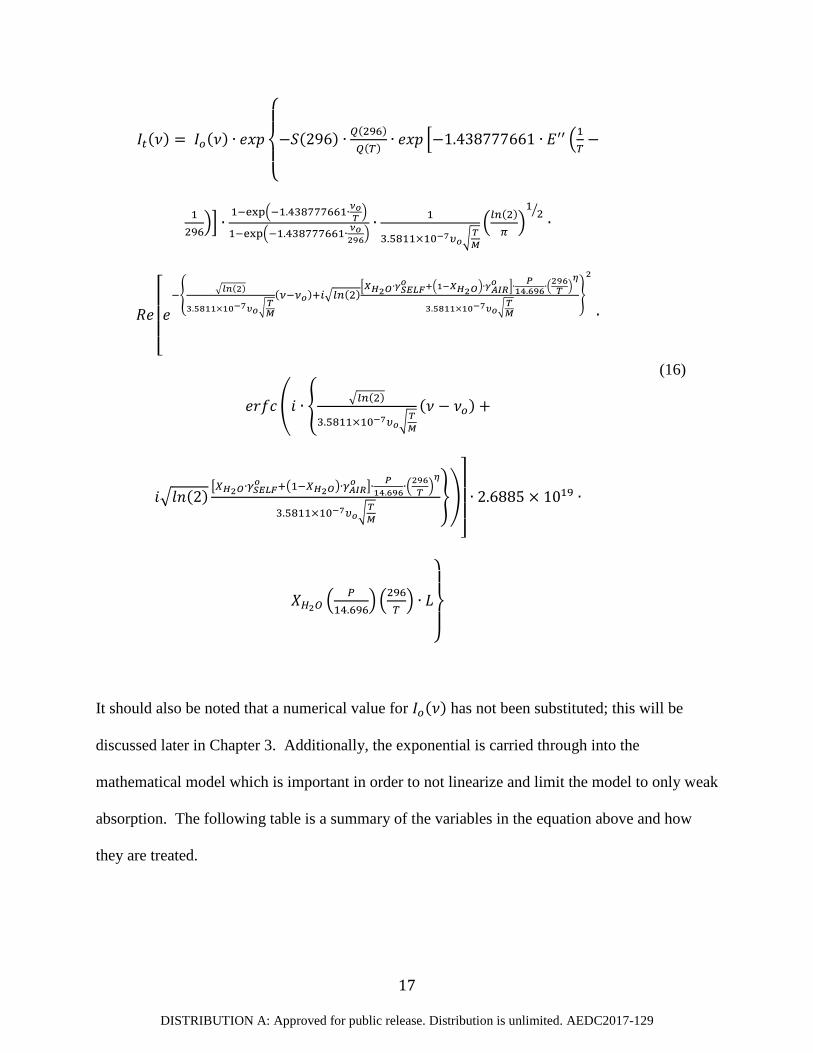
Final Computational Equation
The resultant equation from the previous section, discussed but not shown, is much easier
to evaluate than Equation 13, but more work is required in order to obtain an expression that can
be implemented into code. The expression must be completely expanded, as shown in Equation
16. The first step is to substitute Equations 14, 12, 7, 8, 10 and 15 into Equation 13 to fully
expand all of the terms. The constant in Equation 15 is Loschmidt’s number and represents the
number of molecules in a given volume [cm-3].
𝑁𝑁 = 2.6885 × 10¹⁹ ∙ 𝑋𝑋𝐻𝐻2𝑂𝑂 �𝑃𝑃𝑃𝑃𝑜𝑜� �𝑇𝑇𝑜𝑜𝑇𝑇� (15)
Next, the numerical values for 𝑇𝑇𝑜𝑜, 𝑃𝑃𝑜𝑜, h, c, kB will be substituted into the expanded
equation discussed above leading to the final form of the mathematical model shown below in
Equation 16. This will be implemented into the Spectral Model and Curve Fitting Tools
discussed in the next chapter.
DISTRIBUTION A: Approved for public release. Distribution is unlimited. AEDC2017-129
17
𝐼𝐼𝑡𝑡(𝜈𝜈) = 𝐼𝐼𝑜𝑜(𝜈𝜈) ∙ 𝑒𝑒𝑒𝑒𝑒𝑒
⎩⎪⎨
⎪⎧
−𝑆𝑆(296) ∙ 𝑄𝑄(296)𝑄𝑄(𝑇𝑇) ∙ 𝑒𝑒𝑒𝑒𝑒𝑒 �−1.438777661 ∙ 𝑐𝑐′′ �1
𝑇𝑇−
1296�� ∙
1−exp�−1.438777661∙𝜈𝜈𝑜𝑜𝑇𝑇 �
1−exp�−1.438777661∙ 𝜈𝜈𝑜𝑜296�∙ 1
3.5811×10⁻⁷𝜐𝜐𝑜𝑜�𝑇𝑇𝑀𝑀
�𝑙𝑙𝑙𝑙(2)𝜋𝜋�12� ∙
𝑅𝑅𝑒𝑒
⎣⎢⎢⎢⎡𝑒𝑒−� �𝑙𝑙𝑙𝑙(2)
3.5811×10⁻⁷𝜐𝜐𝑜𝑜�𝑇𝑇𝑀𝑀
(𝜈𝜈−𝜈𝜈𝑜𝑜)+𝑖𝑖�𝑙𝑙𝑙𝑙(2)�𝑋𝑋𝐻𝐻2𝑂𝑂∙𝛾𝛾𝑆𝑆𝑆𝑆𝑆𝑆𝑆𝑆
𝑜𝑜 +�1−𝑋𝑋𝐻𝐻2𝑂𝑂�∙𝛾𝛾𝐴𝐴𝐴𝐴𝐴𝐴𝑜𝑜 �∙ 𝑃𝑃
14.696∙�296𝑇𝑇 �
𝜂𝜂
3.5811×10⁻⁷𝜐𝜐𝑜𝑜�𝑇𝑇𝑀𝑀
�
2
∙
𝑒𝑒𝑒𝑒𝑒𝑒𝑐𝑐 �𝑖𝑖 ∙ � �𝑙𝑙𝑙𝑙(2)
3.5811×10⁻⁷𝜐𝜐𝑜𝑜�𝑇𝑇𝑀𝑀
(𝜈𝜈 − 𝜈𝜈𝑜𝑜) +
𝑖𝑖�𝑑𝑑𝑙𝑙(2)�𝑋𝑋𝐻𝐻2𝑂𝑂∙𝛾𝛾𝑆𝑆𝑆𝑆𝑆𝑆𝑆𝑆
𝑜𝑜 +�1−𝑋𝑋𝐻𝐻2𝑂𝑂�∙𝛾𝛾𝐴𝐴𝐴𝐴𝐴𝐴𝑜𝑜 �∙ 𝑃𝑃
14.696∙�296𝑇𝑇 �
𝜂𝜂
3.5811×10⁻⁷𝜐𝜐𝑜𝑜�𝑇𝑇𝑀𝑀
��
⎦⎥⎥⎥⎤∙ 2.6885 × 10¹⁹ ∙
𝑋𝑋𝐻𝐻2𝑂𝑂 �𝑃𝑃
14.696� �296
𝑇𝑇� ∙ 𝐿𝐿
⎭⎪⎬
⎪⎫
(16)
It should also be noted that a numerical value for 𝐼𝐼𝑜𝑜(𝜈𝜈) has not been substituted; this will be
discussed later in Chapter 3. Additionally, the exponential is carried through into the
mathematical model which is important in order to not linearize and limit the model to only weak
absorption. The following table is a summary of the variables in the equation above and how
they are treated.

DISTRIBUTION A: Approved for public release. Distribution is unlimited. AEDC2017-129
18
Table I: Variables list for Equation 16
Variable Units Definition Treatment 𝐼𝐼𝑜𝑜(𝜈𝜈) W/cm2 Incident intensity Fit Parameter, Provides baseline fit 𝐼𝐼𝑡𝑡(𝜈𝜈) W/cm2 Transmitted intensity Measured by LH system 𝑆𝑆(296) cm-1/(molecules·cm-2) Reference line strength at 296 K Input, HITRAN
𝑄𝑄(296) - Reference internal partition function at 296 K Input, HITRAN
𝑄𝑄(𝑇𝑇) - Temperature dependent internal partition function Known, Interpolated from table
𝑐𝑐′′ cm-1 Lower state energy Input, HITRAN 𝑇𝑇 K Temperature Input, Fit Parameter 𝜈𝜈𝑜𝑜 cm-1 Line center wavenumber Input, HITRAN 𝑀𝑀 g/mol Molar mass Input 𝜈𝜈 cm-1 wavenumber Input, Determined from Etalon Constants
𝑋𝑋𝐻𝐻2𝑂𝑂 mol H2O/ mol air Mole fraction of H2O Input, Fit Parameter 𝛾𝛾𝑆𝑆𝑆𝑆𝐿𝐿𝑆𝑆𝑜𝑜 cm-1/atm Self-broadened HWHM Input, HITRAN 𝛾𝛾𝐴𝐴𝐴𝐴𝐴𝐴𝑜𝑜 cm-1/atm Air-broadened HWHM Input, HITRAN 𝑃𝑃 PSI Static Pressure Input, Fit Parameter
𝜂𝜂 - Coefficient of temperature
dependence of air-broadened HWHM
Input, HITRAN
𝐿𝐿 cm Path length Input

DISTRIBUTION A: Approved for public release. Distribution is unlimited. AEDC2017-129
19
CHAPTER III
SPECTRAL MODEL AND CURVE FITTING TOOL
Spectral Model
In order to select the best absorption transition for the environmental conditions and
design range of the water vapor concentration the sensor is expected to measure, a computational
model using MATLAB and its graphical user interface (GUI) has been created. A screen shot of
the GUI is displayed in the following figure. The purpose of this model is to accurately simulate
the absorption spectrum over a desired wavelength range so the optimal absorption line(s) can be
selected to produce the most accurate humidity measurement.
Figure 3: Absorption Model GUI

DISTRIBUTION A: Approved for public release. Distribution is unlimited. AEDC2017-129
20
This model requires inputs for the environmental conditions which are to be simulated:
temperature, pressure, H2O mole fraction and path length. The spectral resolution, labeled as #
of Points, as well as the lower and upper bound for the wavelength range are also inputs to the
model. The bounds can be input as wavelength [nm] or wavenumber [cm-1]. The GUI includes a
plot selection option that allows the user to toggle between plots of the absorption spectrum (I)
and the absorption coefficient (𝑘𝑘). The button labeled “Run Sim.” computes the absorption
spectrum and absorption coefficient over the selected spectral range for the given input
environmental conditions and water concentration displayed the selected plot in the appropriate
units.
When the GUI is launched, default values for all inputs are already selected. The line
strength from Equation 5 and the Lorentzian linewidth from Equations 7-8 are calculated using
the default values. If any of the environmental inputs are changed, the Lorentzian linewidth is
updated as well. The path length is input in units of feet, but converts into centimeters for
computation. When the lower or upper wavelength bound is changed, the program searches pre-
loaded data from the HITRAN database to find all of the lines within the bounds. In the same
step, the values for the reference line strength, 𝑆𝑆(𝑇𝑇𝑜𝑜), line center frequency, 𝜈𝜈𝑜𝑜, self-broadened
HWHM, 𝛾𝛾𝑆𝑆𝑆𝑆𝐿𝐿𝑆𝑆𝑜𝑜 , air-broadened HWHM, 𝛾𝛾𝐴𝐴𝐴𝐴𝐴𝐴𝑜𝑜 , lower energy state, 𝑐𝑐′′, and the coefficient of
temperature dependence, 𝜂𝜂, are tabulated for each line found within the selected range. Upon
pressing the “Run Sim.” button, the profile for each line within the range is calculated using the
equations from Chapter 2. The lines are then summed spectrally to create the final spectrum
over the specified range.
One very important aspect of the model is that each absorption line is modeled using a
Voigt profile as expressed by Equations 11 and 12 in the previous chapter. The improper

DISTRIBUTION A: Approved for public release. Distribution is unlimited. AEDC2017-129
21
integral in Equation 11 is approximated using Equation 14 as discussed in Chapter 2. However,
as seen in Equation 16, this approximation is still very complicated since it deals with complex
numbers. Thus several algorithms using various mathematical techniques have been developed
over the years to perform the calculation [16] [17] [39] [40] [41]. While some of these
techniques are faster and/or more accurate than others, the Humlicek algorithm [17], named after
the developer, was selected due to its acceptable speed and accuracy. Implementation of this
algorithm into the intensity equation is discussed previously in Chapter 2. A FORTRAN version
of this algorithm [17] was converted into a MATLAB function for use in this work.
Absorption Line Selection
Currently, the HITRAN 2012 database has 12,952 different water absorption features in
the 1.3-1.5 µm band which is of interest in this work due to the combination of strong water
absorption features present and the laser sources that are readily available. Most of the
absorption features overlap and interfere with each other when exposed to certain environmental
conditions. Thus, it is imperative to choose features that will be suitable for measurement over
the range of environmental conditions to which the sensor will be exposed. Literature on LDA
describes systematic procedures for selecting the appropriate absorption lines and is outlined in
papers by H. Li [4] and Farooq [42]. The procedure will vary slightly for each application, thus
the conditions used in this work should be outlined.
The first condition, for the purposes of this study, deals with limiting the wavelength
range of potential lines. This limit is governed by the availability of diode lasers operating
within the 1.3-1.5 µm spectral range where H2O absorption lines are present. The second
condition addresses the line strength. The line strength must be strong enough to allow

DISTRIBUTION A: Approved for public release. Distribution is unlimited. AEDC2017-129
22
measureable absorption, but not so large that the absorption line begins to saturate. The third and
final condition is that the absorption feature must be sufficiently isolated from neighboring
features. This is due to the fact that the analytical model used for the LH assumes a single
absorption transition. If the tails of two features overlap significant errors can develop in the
baseline fit, which is an important part of the fitting process which will be discussed in more
detail in the next section.
Two specific absorption lines 1394.646 nm and 1395.0 nm, lines 10 and 11 respectively
in Figure 4 below, were chosen for this work, based on the three conditions discussed in the
previous paragraph. An illustration follows of how the absorption model GUI and criteria were
use used to select these specific absorption lines. The first condition discusses limiting the
possible absorption lines within the wavelength range of the particular laser used. For this work,
the available diode laser can be tuned safely over the range of approximately 1391 nm and 1397
nm. Operating the laser diode near the upper wavelength limits requires the laser to be operated
near the temperature limits which can cause wavelength instabilities and can shorten the
operational lifetime of the laser diode. The H2O absorption spectrum for this wavelength range
was generated by the spectral model and is displayed in the following figure.

DISTRIBUTION A: Approved for public release. Distribution is unlimited. AEDC2017-129
23
Figure 4: Absorption spectrum for H2O between 1391 nm and 1397 nm at T=300 K, P=14.7 PSI, 𝑋𝑋𝐻𝐻2𝑂𝑂=0.002412 and L=16.0 ft
From this figure, fifteen discernible absorption features that have the potential to be used
are identified within the wavelength constraints. Using condition two, features 3, 5-9 and 13 are
eliminated due to the fact they are too weak. Condition three is now applied to the remaining
features to assess the isolation of each feature. Of the remaining features 2, 4, 12, 14 and 15 all
merge or have significant overlap with other features and are thus not good candidates for use in
this work. This leaves features 1, 10 and 11 as potential candidates for use in the sensor. Further
inspection into feature 1 reveals that an additional weak feature is present on the right wing,
which was not visible in Figure 4 but can be seen in the following figure.
1
2
3
4
5 6 7
8 9
10
11
12
13
14
15

DISTRIBUTION A: Approved for public release. Distribution is unlimited. AEDC2017-129
24
Figure 5: Absorption spectrum for feature 1 at T=300 K, P=14.7 PSI, 𝑋𝑋𝐻𝐻2𝑂𝑂=0.002412 and L=16.0 ft
This newly discovered feature will cause problems when trying to computationally analyze the
profile and lead to significant error in the result. Next, features 10 and 11 were looked at in more
detail to determine if the lines are suitable.
Features 10 and 11, at three different sets of environmental conditions, are displayed
below in order to see how the different conditions affect the shape of each line.
1
Weak Feature

DISTRIBUTION A: Approved for public release. Distribution is unlimited. AEDC2017-129
25
(a)
(b)

DISTRIBUTION A: Approved for public release. Distribution is unlimited. AEDC2017-129
26
(c)
Figure 6: Features 10 and 11, 1394.7 nm and 1395.0 nm respectively, for three different conditions. (a) T=300 K, P=14.7 PSI, 𝑋𝑋𝐻𝐻2𝑂𝑂=0.002412 and L=16.0 ft, (b) T=300 K, P=0.5 PSI,
𝑋𝑋𝐻𝐻2𝑂𝑂=0.0001 and L=16.0 ft and (c) T=300 K, P=27 PSI, 𝑋𝑋𝐻𝐻2𝑂𝑂=0.01 and L=16.0 ft
Figure 6(a) displays the two features at the same atmospheric conditions as Figures 4 and 5. The
environmental conditions the two lines are expected to vary greatly from Figure 6(a). Figure
6(b) illustrates the effect of low pressure and humidity. Additionally, Figure 6(c) displays the
effect of high pressure and humidity. In Figure 6(b), the line at 1394.7nm is too weak. This
technique works best with lines ranging from at least 1% to approximately 80% peak
absorbance. In Figure 6(c), the line at 1395.0nm is saturated. From Figure 6 it can be seen that
one specific feature will not work for the given laser range and environmental conditions. At
lower pressures, feature 10 will become too weak with maximum absorbance occurring around
0.3% and at higher pressures feature 11 will become too broad, spanning over 0.4 nm. To span

DISTRIBUTION A: Approved for public release. Distribution is unlimited. AEDC2017-129
27
the dynamic range in concentration for the required temperature and pressure environmental
conditions both lines must be used. Feature 10 will be used at high pressures and humidity
levels, when feature 11 is too strong and broad. Similarly, feature 11 will be used at low
pressures and humidity levels, when feature 10 becomes too weak and narrow. This will allow
for an optimum line shape under all possible environmental water concentration conditions
expected to occur within the facility. The HITRAN 2012 parameters used to describe these two
lines are listed below.
Table II: HITRAN parameters for the 1394.7 nm and 1395.0 nm absorption lines
Parameter 1394.7 nm Line 1395.0 nm Line 𝜈𝜈𝑜𝑜 7170.27781 7168.43701
𝑆𝑆(𝑇𝑇𝑜𝑜) 1.969E-21 1.170E-20 𝛾𝛾𝐴𝐴𝐴𝐴𝐴𝐴𝑜𝑜 0.0928 0.0956 𝛾𝛾𝑆𝑆𝑆𝑆𝐿𝐿𝑆𝑆𝑜𝑜 0.5 0.473 𝑐𝑐′′ 206.3014 173.3658 𝜂𝜂 0.71 0.71
Curve Fitting Tool
Using the equations presented in Chapter 2, a curve fitting tool has been developed to fit
the computational model to the raw test data. By fitting the environmental parameters,
information regarding the test environment can be obtained. As with the computational model,
MATLAB was used to perform this analysis via the creation of a GUI, which is shown in Figure
7. The GUI was developed for convenience and efficiency since a significant number of data
sets need to be analyzed.

DISTRIBUTION A: Approved for public release. Distribution is unlimited. AEDC2017-129
28
Figure 7: Curve Fitting Tool for raw absorption data
Figure 7 is clearly organized with the inputs located on the top half of the GUI and the outputs
on the bottom half of the GUI.
To begin the analysis of a data set, the raw data must be loaded into the GUI’s workspace
using the Select File button. Once the button is pressed a file explorer will show up on the
screen so that the appropriate data file can be selected. Once the file is selected, the raw data
will be displayed in the plot in the top left corner of the GUI as seen in Figure 8.
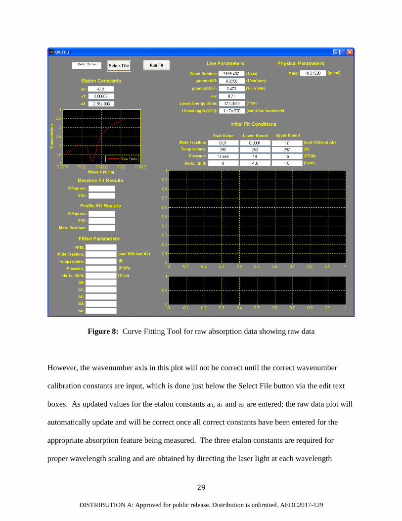
DISTRIBUTION A: Approved for public release. Distribution is unlimited. AEDC2017-129
29
Figure 8: Curve Fitting Tool for raw absorption data showing raw data
However, the wavenumber axis in this plot will not be correct until the correct wavenumber
calibration constants are input, which is done just below the Select File button via the edit text
boxes. As updated values for the etalon constants a0, a1 and a2 are entered; the raw data plot will
automatically update and will be correct once all correct constants have been entered for the
appropriate absorption feature being measured. The three etalon constants are required for
proper wavelength scaling and are obtained by directing the laser light at each wavelength
DISTRIBUTION A: Approved for public release. Distribution is unlimited. AEDC2017-129
30
through a 2.0GHz etalon and measuring the peaks to achieve proper wavelength scaling for the
raw signal generated from the detector. An example of this process is described below.
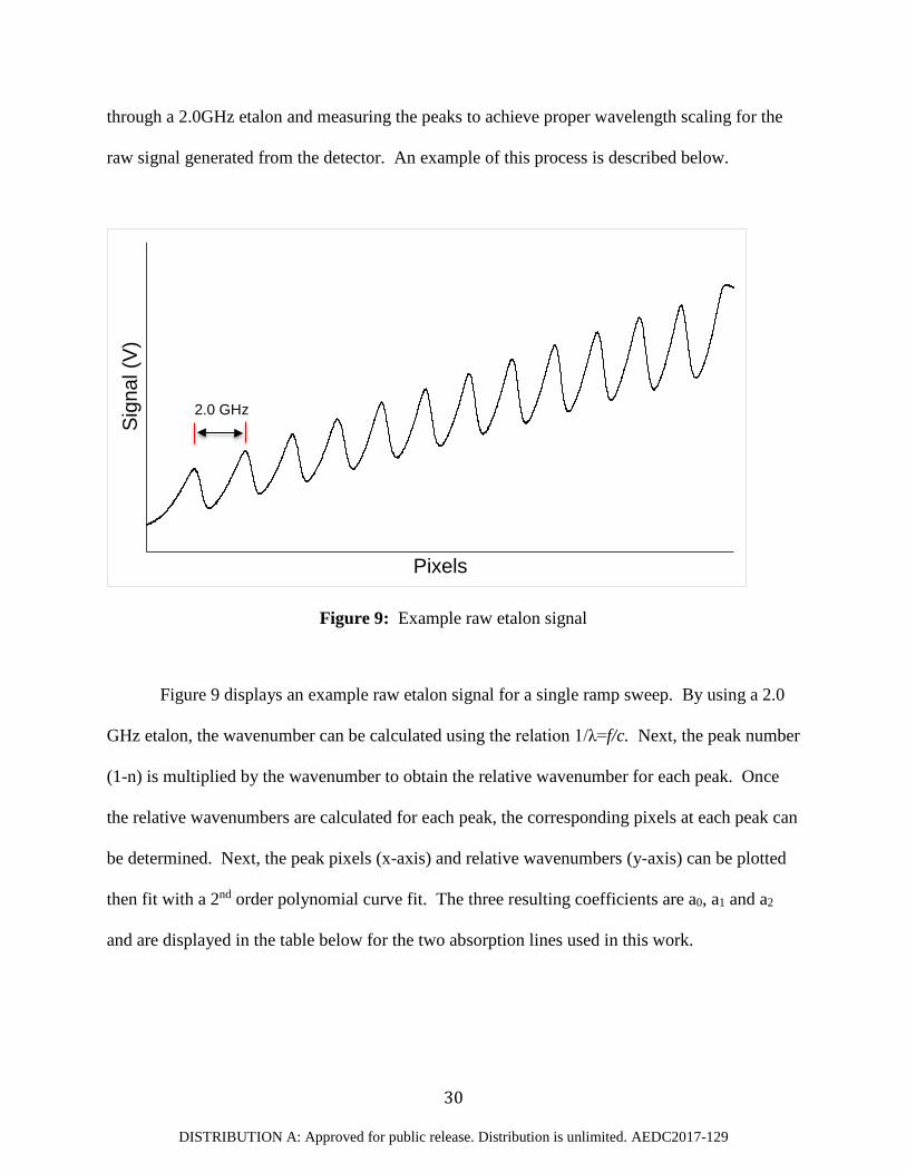
Figure 9: Example raw etalon signal
Figure 9 displays an example raw etalon signal for a single ramp sweep. By using a 2.0
GHz etalon, the wavenumber can be calculated using the relation 1/λ=f/c. Next, the peak number
(1-n) is multiplied by the wavenumber to obtain the relative wavenumber for each peak. Once
the relative wavenumbers are calculated for each peak, the corresponding pixels at each peak can
be determined. Next, the peak pixels (x-axis) and relative wavenumbers (y-axis) can be plotted
then fit with a 2nd order polynomial curve fit. The three resulting coefficients are a0, a1 and a2
and are displayed in the table below for the two absorption lines used in this work.
Sign
al (V
)
Pixels
2.0 GHz

DISTRIBUTION A: Approved for public release. Distribution is unlimited. AEDC2017-129
31
Table III: Etalon constants for the 1394.7 nm and 1395.0 nm absorption lines
Parameter 1394.7 nm Line 1395.0 nm Line a0 -0.95 -0.90 a1 5.46E-3 6.02E-3 a2 -1.27E-6 -2.36E-6
Next, all of the Line and Physical parameters must be checked and entered correctly.
These parameters are constants specific to the particular feature and species selected and are not
a function of the environmental conditions that are being fit. Once all of the parameters are input
and correct, the Initial Fit parameters must be adjusted as needed to ensure an accurate fit. These
parameters represent the environmental conditions that affect the shape of the absorption feature
and that are being fit in the tool, with exception to the wavenumber parameter. The wavenumber
shift parameter has been added to the computational model to account for the wavelength drift of
the laser diode or shift in the absorption line feature due to pressure or Doppler effects. This is
done to create the most accurate fit possible. The Initial Fit Parameters each consist of a start
value, lower bound and upper bound that guide the fit algorithm to most accurate solution
possible.
Typically, the temperature is known to a high degree of accuracy and does not affect the
feature nearly as much as the other parameters, so the upper and lower bounds are set very close
to the start value. In addition, the pressure is also known to a fair degree of accuracy, but a
generous range is usually selected to give the fitting algorithm enough freedom to produce a very
accurate fit. In reality, the temperature and pressure are not unknown, but through trial and error,
it is found that a much better fit is achieved by fitting these two parameters as well. The mole
fraction is obviously the fit parameter in which we are most concerned with. It is unknown and

DISTRIBUTION A: Approved for public release. Distribution is unlimited. AEDC2017-129
32
is very sensitive to the width and height of the feature, thus the upper and lower bounds create a
very broad range for the same reason as the pressure parameter.
The type of fit used for this analysis is a non-linear least squares regression implementing
the “large scale: trust-region reflective Newton” algorithm. Other non-linear least squares
algorithms can be used in MATLAB including “Gauss-Newton” and “Levenberg-Marquardt.”
In the literature, the “Levenberg-Marquardt” algorithm is mentioned most frequently, but for this
work the above mentioned algorithm was used because it produced a much better fit and a more
accurate mole fraction result.
In addition to the computational model itself, a fourth order polynomial fit has been
added to fit the baseline I0. This way the computational model can be applied to the raw data
without error. The polynomial expression is shown below where the 𝑏𝑏 terms are the polynomial
coefficients and ∆𝜈𝜈 is the wavenumber parameter mentioned above.
𝐼𝐼0 = 𝑏𝑏0 + 𝑏𝑏1 ∙ (𝜈𝜈 − 𝜈𝜈0 + ∆𝜈𝜈) + 𝑏𝑏2 ∙ (𝑒𝑒 − 𝜈𝜈0 + ∆𝜈𝜈)2 + 𝑏𝑏3
∙ (𝑒𝑒 − 𝜈𝜈0 + ∆𝜈𝜈)3 + 𝑏𝑏4 ∙ (𝑒𝑒 − 𝜈𝜈0 + ∆𝜈𝜈)4 (17)
The above expression is applied to the computational model by simply substituting the above
expression for 𝐼𝐼0 into Equation 16.
Once all of the inputs are entered the Run Fit button, to the right of the Select File
button, is pressed to perform the fit. Upon completion, the raw data, the fit and the baseline fit
are plotted on the large axis on the right. Also, the Fit results and Fitted Parameters are output to
the left of the axis. The residuals of the raw data and fit data are plotted below the fit results plot
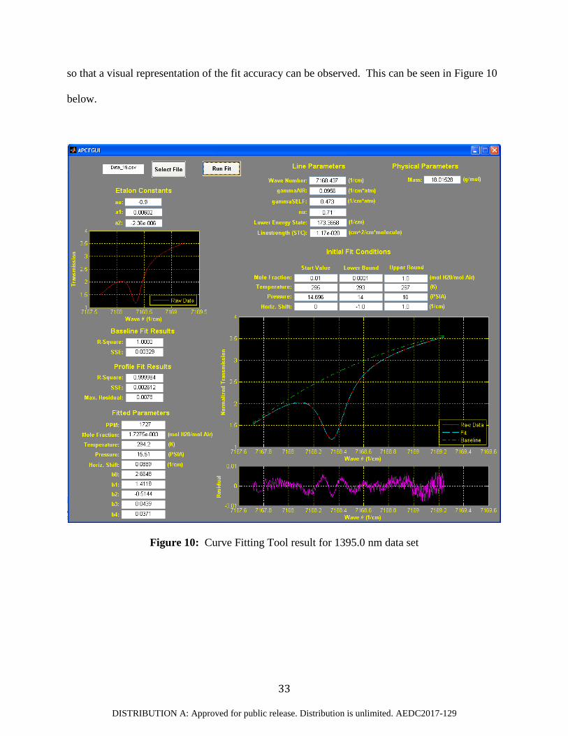
DISTRIBUTION A: Approved for public release. Distribution is unlimited. AEDC2017-129
33
so that a visual representation of the fit accuracy can be observed. This can be seen in Figure 10
below.
Figure 10: Curve Fitting Tool result for 1395.0 nm data set
DISTRIBUTION A: Approved for public release. Distribution is unlimited. AEDC2017-129
34
CHAPTER IV
EXPERIMENTAL SETUP
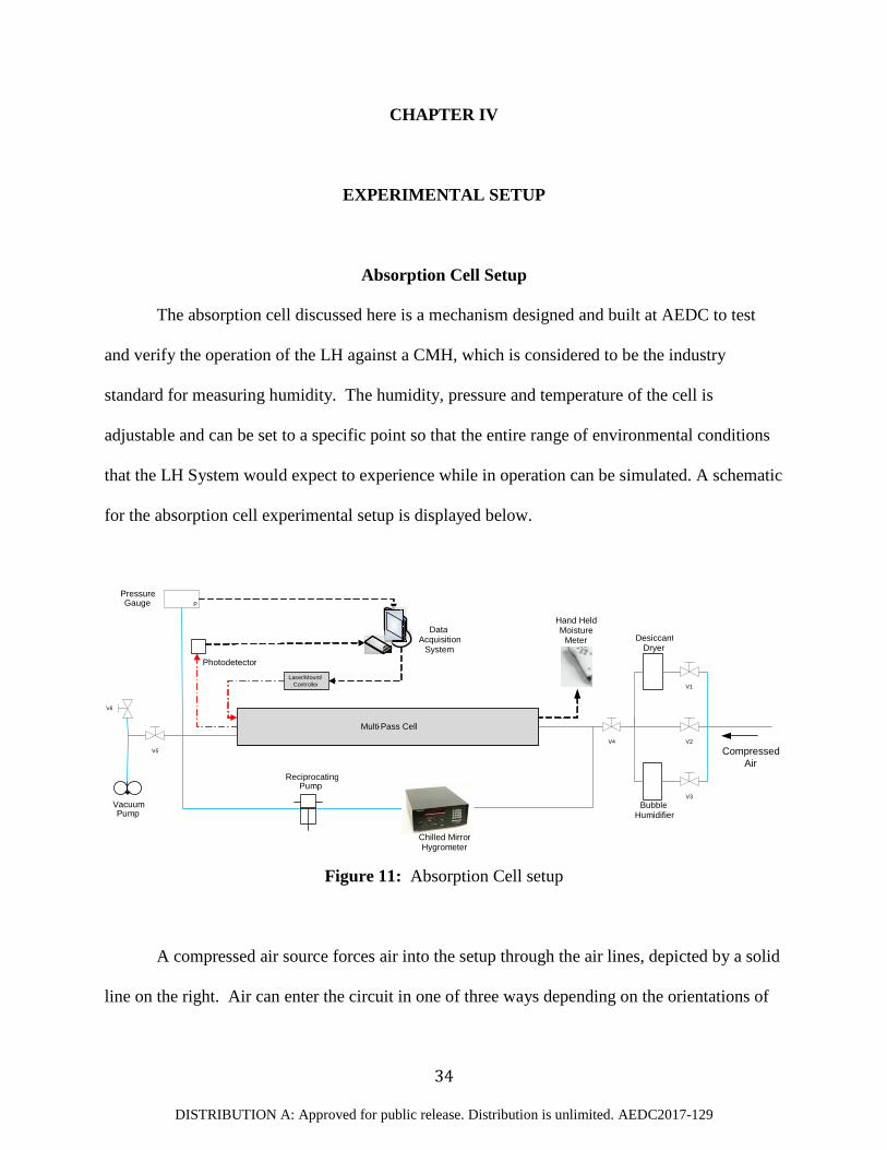
Absorption Cell Setup
The absorption cell discussed here is a mechanism designed and built at AEDC to test
and verify the operation of the LH against a CMH, which is considered to be the industry
standard for measuring humidity. The humidity, pressure and temperature of the cell is
adjustable and can be set to a specific point so that the entire range of environmental conditions
that the LH System would expect to experience while in operation can be simulated. A schematic
for the absorption cell experimental setup is displayed below.
Figure 11: Absorption Cell setup
A compressed air source forces air into the setup through the air lines, depicted by a solid
line on the right. Air can enter the circuit in one of three ways depending on the orientations of
3 V 5 V 4
V 1
V 2
V 3
Compressed Air
V 6 Multi - Pass Cell
Desiccant Dryer
Bubble Humidifier
Reciprocating Pump
Vacuum Pump
Data Acquisition
System Photodetector
P Pressure Gauge
Chilled Mirror Hygrometer
Hand Held Moisture
Meter
Laser/Mount / Controller
DISTRIBUTION A: Approved for public release. Distribution is unlimited. AEDC2017-129
35
valves V1-V3. If the air travels through valve V1, it passes through a desiccant dryer to reduce
the amount of water vapor in the air. If air passes through V2 it enters the circuit unconditioned.
If the air passes through valve V3, moisture is added to the air by a bubble humidifier. The
conditioned/unconditioned air then travels through valve V4 to enter the circuit.
While conducting an absorption experiment, valve V4 will be closed to ensure the
environmental conditions within the circuit will not change. The air is then circulated through
the multi-pass cell, which has a total path length of 16 ft, by a reciprocating pump manufactured
by Air Control, Inc. This is done to achieve a homogenous humidity level throughout the circuit.
The pump is allowed to run for several minutes before any measurements are taken to ensure
homogeneity. As the air circulates it passes through a Dew Prime III Chilled Mirror Hygrometer
manufactured by EdgeTech, where the dew point of the air is measured. The pressure of the cell
is measured by a PX32B1-050AV pressure transducer manufactured by OMEGADYNE, Inc.
and displayed by a DP25B-S-A pressure Indicator manufactured by Omega Engineering, Inc.;
both of which are represented by a single block in Figure 8. Valve V5 is used in the same
manner as valve V4 while an experiment is being conducted, but can be opened so that a vacuum
can be put on the circuit by a two stage vacuum pump, manufactured by Edwards, or the circuit
can be exhausted to the atmosphere using valve V6. This allows for the pressure in the cell to be
lowered or a vacuum to be applied. Valves V4 and V5 in combination with the compressed air
supply and vacuum pump allow for complete pressure control of the circuit.
The tunable diode laser source produces continuous-wave radiation over an infrared
spectral range of 1391-1397 µm which is contained and directed into the multi-pass cell using a
single mode fiber optic cable, depicted by the dash-dot line. The signal beam is coupled into a
50 µm diameter, multimode fiber and routed to an InGaAs-PIN photodiode. The transmit and

DISTRIBUTION A: Approved for public release. Distribution is unlimited. AEDC2017-129
36
receive fibers are both routed through a vacuum tight fitting installed on the absorption cell. The
detector converts the optical signal into an electrical signal that travels to the data acquisition
system (DAQ) via a National Instruments (NI) terminal block, TB-2709, which is directly
connected to the NI DAQ model PXI-6123 analog to digital converter. The DAQ system is a 16
bit system capable of simultaneously measuring 8 separate channels at a rate of 500 KS/s,
although only two channels were used in this work, raw data and pressure. The laser diode and
temperature controller mount are a single unit, model LDCM-4371, manufactured by PSE
Technology, which are controlled the by the DAQ computer as well. The injection current to the
laser diode is modulated by a function generator using a sawtooth ramp. Temperature is
manually input into the data acquisition system based on ambient room conditions and is
considered to be a constant. An additional multi-pass cell humidity measurement is performed
by a Hand-Held humidity and Temperature meter, model MM70, manufactured by Vaisala for
comparison with CMH and LH.
Sensor Calibration Setup
Once it was confirmed that the LH functioned correctly using the lab absorption cell,
described in the previous section, a calibration using a National Institute of Standards and
Technology (NIST) traceable HG was performed. The experimental setup for the Precision
Measurement Equipment Lab (PMEL) calibration is displayed below and will be discussed in
further detail below.

DISTRIBUTION A: Approved for public release. Distribution is unlimited. AEDC2017-129
37
Figure 12: PMEL calibration setup
The humidity source is a Thunder Scientific Model 3900 “Two-Pressure Two-Temperature”
Low Humidity Generator that is traceable to NIST. Once the desired dew point is set, the
humidity source will begin producing air with the desired level of humidity. However, it does
take the humidity source and absorption cell several hours to stabilize at the desired condition at
the lower humidity levels. The air produced by the humidity source is directed into the
calibration cell which is the same cell as used in the absorption cell setup. The air from the cell
flows through a CMH and vented to the atmosphere. Once the humidity source and the CMH
both stabilized a data point could be taken with the LH. The LH, in the above figure, is the same
system used in the absorption cell setup and is described there.
Wind Tunnel System Setup
The actual operational system used in the wind tunnel is only a portion of what was seen
in the Absorption Cell setup. The schematic for the operational system is shown in Figure 13.
Multi - Pass Cell V - 1
Data Acquisition
System Photodetector
Chilled Mirror Hygrometer
Laser/Mount / Controller

DISTRIBUTION A: Approved for public release. Distribution is unlimited. AEDC2017-129
38
StillingChamber
Ts, Ps
Data Acquisition
SystemPhotodetector
Laser Mount/Controller
Figure 13: LH System setup
The laser diode and controller mount are the same as in the Absorption Cell and PMEL
calibration setups. The beam is delivered to the wind tunnel via the same single mode optical
fiber as in the absorption cell and calibration setups and is indicated by the dash-dot line. The
exposed beam passes through the wind tunnel onto a photodiode which converts the laser beam
into an analog signal and directs that signal into the same DAQ as in the absorption cell and
calibration setups. It should also be noted that there are no pressure transducers or
thermocouples displayed in Figure 13, this is because the static pressure and temperature are sent
to the DAQ from the facility DAQ through a server.
4T /

DISTRIBUTION A: Approved for public release. Distribution is unlimited. AEDC2017-129
39
CHAPTER V
EXPERIMENTAL RESULTS AND DISCUSSION
Absorption Cell Results
The first step in experimentation is to verify the operation of the LH which was done
using the Absorption Cell described in Chapter 4. Figure 14 displays the LH results compared to
the Viasala hand-held meter.
Figure 14: Mole fraction data for the Vaisala hand-held meter (2 channels) and LH for the 1394.7 nm absorption line
1
2
3
4
5
6
7Absorption Cell Sensor Comparison
Mol
e Fr
actio
n (x
103 )
Viasala 1Viasala 2LH
Vaisala 1 Vaisala 2

DISTRIBUTION A: Approved for public release. Distribution is unlimited. AEDC2017-129
40
From Figure 14, it appears that Vaisala 1, Vaisala 2 and the LH agree at the lower humidity
levels but the LH begins to differ from the Vaisala1, Vaisala 2 measurements as humidity level
increases. It can also be seen that the LH consistently measures lower values than the Vaisala
sensors.
Figure 14 shows that the LH and Vaisala measurements show the same trend, but there is
discrepancy between instruments. Figure 15 shows this in more detail by comparing each of the
Vaisala sensors to the LH.
Figure 15: Vaisala/LH comparison for the Vaisala hand-held measurements for the 1394.7 nm absorption line
It can be seen in Figure 15 that all of the ratios are above 1, indicating the Vaisala sensors
measure a higher humidity for the entire range of mole fractions seen in Figure 14. Additionally,
1 1.5 2 2.5 3 3.5 4 4.5 5 5.5 61.02
1.04
1.06
1.08
1.1
1.12
1.14
1.16
1.18Ratio of Viasala to LH
LH (Mole Fraction x103)
Via
sala
/LH
Viasala 1/LHViasala 2/LH
Vaisala 1/LH Vaisala 2/LH

DISTRIBUTION A: Approved for public release. Distribution is unlimited. AEDC2017-129
41
there appears to be more variability in the Vaisala measurements at lower humidity levels and
less variability as humidity is increased. This shows that the Vaisala cannot precisely measure
humidity in the 1,000 PPM range.
It was initially thought that the Vaisala hand-held meter would measure humidity
accurately in the ranges created in the absorption cell, but its measurement discrepancy with the
LH and its variability at lower humidity levels indicate otherwise. However, the same general
trend is displayed with both the LH and the Vaisala hand-held meter. This provides confidence
that the LH is operating correctly, but nothing can be concluded in terms of accuracy since there
is no evidence that either device is correct. The next step is to add a CMH to the cell and
compare the LH measurements to the CMH, which is considered the most accurate commercial
humidity measurement device on the market.
Figure 16: Mole fraction data for the LH and CMH for the 1394.7 nm absorption line
0
5
10
15
20
25
30Absorption Cell Comparison of CMH and LH
Mol
e Fr
actio
n (x
103 )
CMHLH
DISTRIBUTION A: Approved for public release. Distribution is unlimited. AEDC2017-129
42
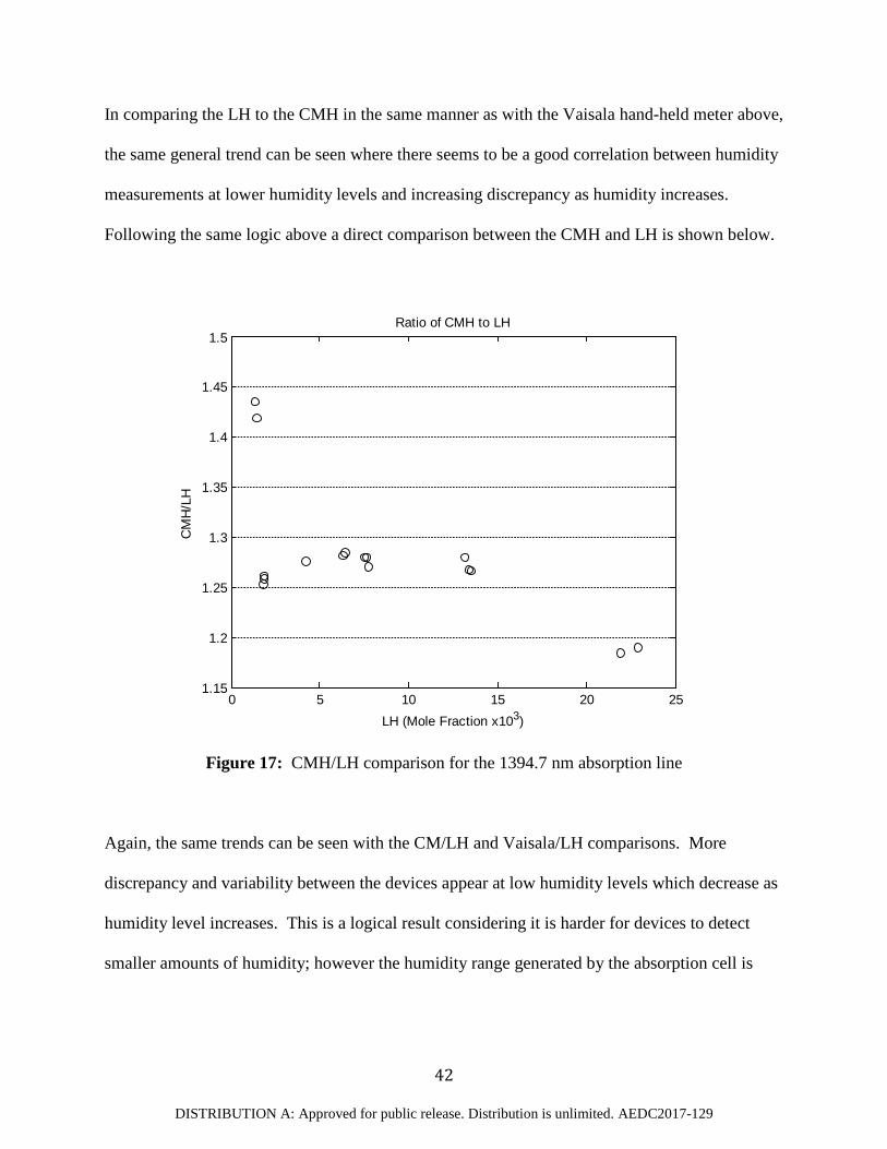
In comparing the LH to the CMH in the same manner as with the Vaisala hand-held meter above,
the same general trend can be seen where there seems to be a good correlation between humidity
measurements at lower humidity levels and increasing discrepancy as humidity increases.
Following the same logic above a direct comparison between the CMH and LH is shown below.
Figure 17: CMH/LH comparison for the 1394.7 nm absorption line
Again, the same trends can be seen with the CM/LH and Vaisala/LH comparisons. More
discrepancy and variability between the devices appear at low humidity levels which decrease as
humidity level increases. This is a logical result considering it is harder for devices to detect
smaller amounts of humidity; however the humidity range generated by the absorption cell is
0 5 10 15 20 251.15
1.2
1.25
1.3
1.35
1.4
1.45
1.5Ratio of CMH to LH
LH (Mole Fraction x103)
CM
H/L
H

DISTRIBUTION A: Approved for public release. Distribution is unlimited. AEDC2017-129
43
indicative of the environment the sensor would experience in operation so no information
regarding the accuracy of the LH can be determined from the absorption cell measurements.
Overall the absorption cell measurements were successful in verifying that the LH device
is operating correctly by the trend agreement with the Vaisala and CMH devices. However, with
the Vaisala hand-held device measuring roughly 3-31% higher than the LH and the CMH
measuring roughly 18-43% higher than the LH indicates that one or both of the devices is not
accurate. Thus, a more thorough study of the accuracy of the LH device and possible calibration
is required.
Sensor Calibration Results
The LH was calibrated over a 𝑋𝑋𝐻𝐻2𝑂𝑂 range from 0.00004 to 0.01255. The 1394.7 nm
absorption line was used for a 𝑋𝑋𝐻𝐻2𝑂𝑂 range of 0.00031 to 0.01255 and the 1395.0 nm absorption
line was used for a lower 𝑋𝑋𝐻𝐻2𝑂𝑂 range of 0.00004 to 0.01255. Figure 18 shows the LH
measurements at the HG set points.
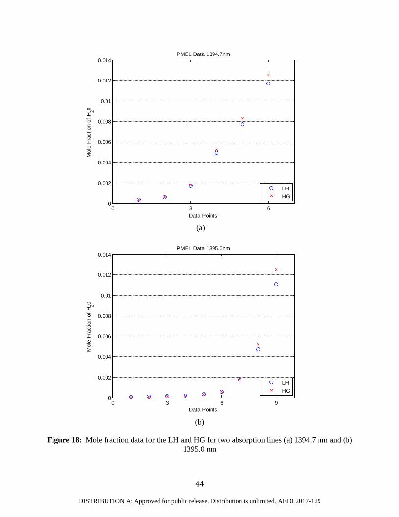
DISTRIBUTION A: Approved for public release. Distribution is unlimited. AEDC2017-129
44
(a)
(b)
Figure 18: Mole fraction data for the LH and HG for two absorption lines (a) 1394.7 nm and (b)
1395.0 nm
0 3 60
0.002
0.004
0.006
0.008
0.01
0.012
0.014
Data Points
Mol
e Fr
actio
n of
H20
PMEL Data 1394.7nm
LHHG
0 3 6 90
0.002
0.004
0.006
0.008
0.01
0.012
0.014
Data Points
Mol
e Fr
actio
n of
H20
PMEL Data 1395.0nm
LHHG

DISTRIBUTION A: Approved for public release. Distribution is unlimited. AEDC2017-129
45
From Figure 18, it appears there is good agreement between the LH and the HG. However, as
the humidity level increases the LH under predicts the mole fraction for both absorption lines. To
get a better look at the agreement between the two sources they can be plotted against each other
using a log-log plot and a linear fit can be applied to see how close they actually agree.
(a)
0.0001 0.001 0.01 0.10.0001
0.001
0.01
0.1
y=0.93007x+5.7668e-005
HG (mole fraction)
LH (m
ole
fract
ion)
LH vs HG Mole Fraction for 1394.7nm
LH vs HG1:1 LineLinear Regression

DISTRIBUTION A: Approved for public release. Distribution is unlimited. AEDC2017-129
46
(b)
Figure 19: Log-Log plot of LH vs. HG for the two absorption lines (a) 1394.7 nm and (b)
1395.0 nm
From the linear fits it can be seen that the LH measurement using the 1394.7 nm line is in closer
agreement with the HG. The slope over the entire humidity range of each line is 0.9301 and
0.8827 respectively. The 1394.7 nm line strength is 6X weaker than the 1395.0 nm line so it
cannot measure as small of a mole fraction as the 1395.0 nm line, but over the range of mole
fractions that were measured it has better agreement. It can be seen in Figure 19(b) that when
the mole fraction drops below 0.0005, the LH response becomes non-linear and the relative error
increases as the humidity decreases. It also appears that not only is the LH under-predicting at
higher mole fractions, the LH is over-predicting at the lower mole fractions. This can be seen by
comparing the data points and linear regression line with the 1:1 line in Figure 19 above.
0.0001 0.001 0.01 0.1
0.0001
0.001
0.01
0.1
y=0.88269x+5.5534e-005
HG (mole fraction)
LH (m
ole
fract
ion)
LH vs HG Mole Fraction for 1395.0nm
LH vs HG1:1 LineLinear Regression
DISTRIBUTION A: Approved for public release. Distribution is unlimited. AEDC2017-129
47
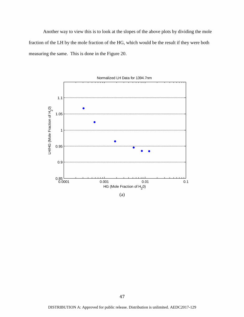
Another way to view this is to look at the slopes of the above plots by dividing the mole
fraction of the LH by the mole fraction of the HG, which would be the result if they were both
measuring the same. This is done in the Figure 20.
(a)
0.0001 0.001 0.01 0.10.85
0.9
0.95
1
1.05
1.1
HG (Mole Fraction of H20)
LH/H
G (M
ole
Frac
tion
of H
20)
Normalized LH Data for 1394.7nm

DISTRIBUTION A: Approved for public release. Distribution is unlimited. AEDC2017-129
48
(b)
Figure 20: LH/HG vs. HG for (a) 1394.7 nm and (b) 1395.0 nm
From Figure 20, the same trend noticed in Figure 18 can be viewed in more detail. The LH
consistently over predicts mole fraction below approximately 0.001 and consistently under
predicts mole fraction above 0.001 for both absorption lines. As the mole fraction drops below
approximately 0.0016, the 1395.0 nm line begins to grossly over predict the mole fraction.
However, the LH using both absorption lines under predict within 10% of the HG over the entire
range of points taken above a mole fraction of 0.001 except for the highest mole fraction
measurement for the 1395.0 nm line.
To correct this, the linear fit shown in Figure 19 above can be used to calibrate the LH.
With a slope of 1 being perfectly calibrated, the linear fit can be converted into a calibration
function by solving for x. The resulting calibration functions are shown below.
0.0001 0.001 0.01 0.10.8
1
1.2
1.4
1.6
1.8
2
HG (Mole Fraction of H20)
LH/H
G (M
ole
Frac
tion
of H
20)
Normalized LH Data for 1395.0nm
DISTRIBUTION A: Approved for public release. Distribution is unlimited. AEDC2017-129
49
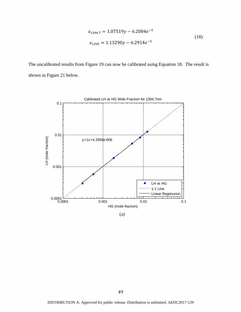
𝑒𝑒1394.7 = 1.07519𝑦𝑦 − 6.2004𝑒𝑒−5
𝑒𝑒1395 = 1.13290𝑦𝑦 − 6.2914𝑒𝑒−5 (18)
The uncalibrated results from Figure 19 can now be calibrated using Equation 18. The result is
shown in Figure 21 below.
(a)
0.0001 0.001 0.01 0.10.0001
0.001
0.01
0.1
y=1x+4.3359e-006
HG (mole fraction)
LH (m
ole
fract
ion)
Calibrated LH vs HG Mole Fraction for 1394.7nm
LH vs HG1:1 LineLinear Regression

DISTRIBUTION A: Approved for public release. Distribution is unlimited. AEDC2017-129
50
(b)
Figure 21: Log-Log plot of Calibrated LH vs. HG for the two absorption lines (a) 1394.7 nm
and (b) 1395.0 nm
From Figure 21, the slope of the linear fit is now 1 indicating the calibration was successful in
correcting the trend of LH overshoot at lower mole fraction and undershoot at higher mole
fraction as discussed previously. However, it can be seen that some of the data points still do not
fall along the fit line. This suggests that there is still some error associated with the system that
cannot be calibrated out.
The remaining error can be broken down into two components: systematic, which
quantifies error in the experiment or instruments used to make the measurements, and random
error, which quantifies unknown changes or fluctuations in the experiment that cannot be
predicted. Both types of error are present in the calibration and will be considered. The
systematic error originates from the HG and is given by the manufacturer. The random error
0.0001 0.001 0.01 0.1
0.0001
0.001
0.01
0.1
y=1x+7.3799e-006
HG (mole fraction)
LH (m
ole
fract
ion)
Calibrated LH vs HG Mole Fraction for 1395.0nm
LH vs HG1:1 LineLinear Regression

DISTRIBUTION A: Approved for public release. Distribution is unlimited. AEDC2017-129
51
originates from the linear curve fit discussed above. The total uncertainty can be calculated by
squaring the systematic and random errors, adding them, then taking the square root. The
following table shows the 𝑋𝑋𝐻𝐻2𝑂𝑂 error values and the total 𝑋𝑋𝐻𝐻2𝑂𝑂 uncertainty for this calibration
procedure.
Table IV: Error component and total uncertainty values for PMEL calibration
Systematic Error Random Error Total Uncertainty 1394.7 nm line 8.9359E-6 6.5669E-6 1.1089E-5 1395.0 nm line 8.9359E-6 1.5522E-5 1.7910E-5
The total uncertainty reported above indicates the PMEL calibration is accurate to a 𝑋𝑋𝐻𝐻2𝑂𝑂 of
±1.1089E-5 for the 1394.7 nm line and ±1.7910e-5 for the 1395.0 nm line or approximately 11
and 18 PPM respectively.
It should also be noted that the CMH’s have a dew point temperature measurement
accuracy of ±0.2ºC (±0.36ºF), as stated in the operator’s manual. This equates to a 𝑋𝑋𝐻𝐻2𝑂𝑂
uncertainty of ±0.000087 or ±87 PPM at a total pressure and temperature of 1 atm and 75ºF
respectively, which is typical for the 4T tunnel. However, through extensive testing at AEDC a
dew point uncertainty of ±2ºF has been observed at best. This equates to a 𝑋𝑋𝐻𝐻2𝑂𝑂 uncertainty of
±0.000481 or ±481 PPM at the same total conditions stated in the previous sentence.
From the PMEL results in Figure 19, it can be seen that the LH curve fitting tool has
difficulty in fitting the absorption at very low and very high absorbance. For low humidity, the
absorption signal is weak and the baseline noise degrades the fitting process. At high humidity
levels, the absorption signal begins to saturate and interference from adjacent lines corrupt the
baseline and degrade the curve fit since only one absorption feature is being analyzed.
DISTRIBUTION A: Approved for public release. Distribution is unlimited. AEDC2017-129
52
The LH should be designed using an absorption line with larger line strength, the 1395.0
nm line, to measure the smaller mole fraction conditions and switch to a weaker absorption line,
the 1394.7 nm line, to measure larger mole fraction conditions to prevent detector saturation.
Thus, the number of different absorption lines used in the system design depends on the mole
fraction range your sensor would be exposed to. Ideally, the sensor would be designed so that
only one absorption line would be needed to cover the range of mole fractions the system would
observe, however the larger the mole fraction range the lower the probability of using one
absorption line is. This is why the absorption model is such an important tool in designing a LH
so that mole fraction range limitation can be tested for each absorption line.
Wind Tunnel System Results
Based on the expected levels of water vapor and the PMEL results, the 1394.7 nm line
was selected for use in AEDC’s 4T wind tunnel. Details regarding the experimental set-up were
previously discussed in Chapter 4. The raw and calibrated LH data are discussed below along
with the calibration method and compared to the values from the CMHs currently installed and
in use. The data was obtained during a wind tunnel test over a Mach number range from 0.9 to
2.5 where numerous different test conditions were set.
Figure 22 shows the calibrated LH and averaged CMH measurements for the AEDC 4T
wind tunnel.

DISTRIBUTION A: Approved for public release. Distribution is unlimited. AEDC2017-129
53
Figure 22: 4T mole fraction date for Averaged CMH and Calibrated LH
In comparing the averaged CMH and calibrated LH measurements, it can be seen that there is
good agreement between the two systems over the entire range of mole fractions. Following the
same logic as in the previous section, the two systems can now be plotted against each other and
a linear fit can be applied to see how closely they actually agree.
0 3 6 91
1.5
2
2.5
3
3.5
4
4.5
5
Data Points
Mol
e Fr
actio
n (x
103 )
4T Mole Fraction Data for Averaged CMH and Calibrated LH
Averaged CMHCalibrated LH

DISTRIBUTION A: Approved for public release. Distribution is unlimited. AEDC2017-129
54
Figure 23: Calibrated LH vs. Averaged CMH mole fraction measurements
The calibrated LH is now measuring within approximately 2% of the CMH. This is a very
promising result considering the CMH values shown are averaged and do contain variability
within themselves. This result does verify that the LH system is quite capable of making
accurate flow humidity measurements. In addition, this result demonstrates an instrument
calibration against a NIST traceable humidity source. System calibration will likely only need
to be performed once every year for each absorption line used unless the system is used to make
measurements in different humidity conditions.
1 1.5 2 2.5 3 3.5 4 4.51
1.5
2
2.5
3
3.5
4
4.5
y=0.9792x+0.075948
Averaged CMH (Mole Fraction x103)
Cal
ibra
ted
LH (M
ole
Frac
tion
x103 )
Calibrated LH vs Averaged CMH Mole Fraction Measurements
Calibrated LH vs Averaged CMH1:1 LineLinear Regression
DISTRIBUTION A: Approved for public release. Distribution is unlimited. AEDC2017-129
55
CHAPTER VI
CONCLUSION
Summary of Research and Results
The work contained within this thesis represents the incremental development of an LH
system. The work began with the selection of an absorption line through the development of an
absorption model. Next a non-linear regression analysis algorithm was created and used to
validate the system using data from the lab absorption cell. The system was then calibrated using
a NIST traceable HG in AEDC’s PMEL and demonstrated in a transonic wind tunnel (AEDC
Propulsion Wind Tunnel 4T).
The two lines selected for experimentation were the 1394.7 nm and 1395.0 nm lines
based on the three conditions discussed in Chapter 3 through the use of the absorption model.
The first condition considered limiting wavelength range based on available laser(s) and their
wavelength ranges. The second condition considered the strength of the line to ensure the
selected line would not be too weak or strong. The third and final condition considered spectral
line isolation to ensure a neighboring line would not induce error into the fit. The Curve Fitting
Tool, utilizing a Voigt line shape model, was then constructed and its operation was verified
using the lab absorption cell. Further work was done to refine and increase the accuracy of the
algorithm which was then calibrated against a NIST traceable HG.
The LH system was taken to AEDC’s PMEL where a calibration was performed using a
NIST traceable HG over a 𝑋𝑋𝐻𝐻2𝑂𝑂 range from 0.00004 to 0.01255. The raw LH data had
approximately a 7% and 12% deviation from the HG data for the 1394.7 nm and 1395.0 nm

DISTRIBUTION A: Approved for public release. Distribution is unlimited. AEDC2017-129
56
lines, respectively. Two trends in the data emerged, the over prediction of the LH at mole
fractions below approximately 𝑋𝑋𝐻𝐻2𝑂𝑂=0.001 and under prediction of the LH at mole fractions
above approximately 𝑋𝑋𝐻𝐻2𝑂𝑂=0.001. The cause of the over prediction is unknown, but the under
prediction is thought to be caused by error in the baseline fit. Both trends were successfully
calibrated out. Additionally, an uncertainty analysis was performed and resulted in a total
uncertainty of 11 to 18 PPM for the 1394.7 nm and 1395.0 nm lines respectively.
The last step was to use the calibrated LH system to make humidity measurements in a
large scale wind tunnel. This was done in the stilling chamber of AEDC’s 4T wind tunnel along
with the CMH system and the measured amount of humidity recorded by the LH system fell
within approximately 2% of the CMH. This is a very good result showing close correlation to the
CMH system which makes the LH technique a very attractive option to measure humidity in 4T.
The major remaining unanswered question is how accurate is the CMH when used in this manner
and is the LH technique even more accurate? The first question is extremely difficult to answer
because there is no exact way to measure the water content in an operational wind tunnel. Thus,
when the LH is compared to the CMH and a 2% difference is observed, how does one determine
if the CMH system is most accurate? Is it possible that the LH system with 2% error is more
accurate? Many scholars and experts in the field would argue that they believe the LH technique
is more accurate, but proving that is beyond the scope of this work.
Despite these questions, there are several advantages to the LH system. First, it makes
in-situ measurements which prevents errors associated with extracting a sample of the flow and
routing it through tubing to the measurement system, unlike the CMH. This also results in the
LH system being much simpler since there are no external tubes to troubleshoot for leaks. The
DISTRIBUTION A: Approved for public release. Distribution is unlimited. AEDC2017-129
57
LH system also is more reliable that the CMH system since it does not rely on mirrors that
occasionally get dirty and have to go offline to be cleaned.
In conclusion, this work has demonstrated that both systems measure humidity to nearly
the same level of accuracy. However, the LH does it using a much simpler and reliable platform.
The combination of these attributes make the LH system a very attractive candidate for an
operational humidity measurement in AEDC’s PWT facilities and possibly beyond.
Future Plans and Recommendations
The next step for this work is to continue moving towards a thoroughly tested operational
system by merging the data analysis code with a data acquisition system. Once that task has been
successfully completed and tested, the system will be capable of making near real-time
measurements on the order of 0.5 seconds. Next, the system must be automated so that once the
system is triggered it will record data, analyze the data, return a humidity measurement result
and repeat the task at a pre-described frequency without error. Lastly, the system will need to be
extensively tested for robustness. In order for the sensor to be solely used during an actual wind
tunnel test, it must be robust and dependable; operating for hours on end without failure or error.
DISTRIBUTION A: Approved for public release. Distribution is unlimited. AEDC2017-129
58
REFERENCES
[1] R. Hanson, "Combustion Gas Measurements Using Tunable Laser Absorption Spectroscopy," in 17th Aerospace Sciences Meeting, New Orleans, 1979. 79-0086.
[2] D. S. Baer, V. Nagali, E. R. Furlong and R. K. Hanson, "Scanned- and Fix-Wavelength Absorpotion Diagnostics for Combustion Measurements Using Multiplexed Diode Lasers," AIAA Journal, vol. 34, no. 3, pp. 489-493, 1996.
[3] V. Nagali, J. Herbon, D. Horning, R. Bates, D. F. Davidson and R. K. Hanson, "Diode-Laser Based Diagnostic to Monitor Water-Vapor in High Pressure Environments," in 37th AIAA Aerospace Sciences Meeting and Exhibit, Reno, 1999. 99-0942.
[4] H. Li, A. Farooq, J. Jeffries and R. K. Hanson, "Near-infrared diode laser absorption sensor for rapid measurements of temperature and water vapor in a shock tube," Applied Physics B - Lasers and Optics, vol. 89, pp. 407-416, 2007.
[5] M. E. Newfield, M. P. Loomis, N. K. J. M. Gopaul, A. Ghorbani, T. R. Kowalski and J. A. Cavolowsky, "Optical Fiber Applications of Laser Absorption Diagnostics in Scramjet Combustors," in 32nd Aerospace Sciences Meeting, Reno, 1994. 94-0386.
[6] J. T. Liu, G. B. Rieker, J. B. Jeffries, M. R. Gruber, C. D. Carter, T. Mathur and R. K. Hanson, "Near-infrared diode laser absorption diagnostic for temperature and water vapor in a scramjet combustor," Applied Optics, vol. 44, no. 31, pp. 6701-6711, 2005.
[7] J. A. Silver and D. J. Kane, "Diode laser measurements of concentration and temperature in microgravity combustion," Measurement Science and Technology, vol. 10, pp. 845-852, 1999.
[8] S. T. Sanders, D. W. Mattison, T. M. Muruganandam and R. K. Hanson, "Multiplexed Diode-Laser Absorption Sensors for Aeropropulsion Flows," in 39th Aerospace Sciences Meeting & Exhibit, Reno, 2001. 2001-0412.
[9] L. S. Chang, J. B. Jeffries and R. K. Hanson, "Mass Flux Sensing via Tunable Diode Laser Absorption of Water Vapor," AIAA Journal, vol. 48, no. 11, pp. 2687-2693, 2010.
[10] L. S. Chang, J. B. Jeffries and R. K. Hanson, "Mass Flux Sensing via Tunable Diode Laser Absorption of Water Vapor," in 48th AIAA Aerospace Sciences Meeting, Orlando, 2010. 2010-303.
[11] L. S. Chang, "Development of a Diode Laser Sensor for Measurement of Mass Flux in Supersonic Flow," Ph.D. Dissertation, Mechanical Engineering Dept., Stanford University, Stanford, CA, 2011.

DISTRIBUTION A: Approved for public release. Distribution is unlimited. AEDC2017-129
59
[12] L. S. Chang, C. L. Strand, J. B. Jeffries and R. K. Hanson, "Supersonic Mass-Flux Measurements via Tunable Diode Laser Absorption and Nonuniform Flow Modeling," AIAA Journal, vol. 49, no. 12, pp. 2783-2791, 2011.
[13] P. R. Wiederhold, "The Principles of Chilled Mirror Hygrometry," Sensors Magazine, pp. 46-51, July 2000.
[14] M. G. Allen, "Diode laser absorption sensors for gas-dynamic and combustion flows," Measurement Science and Technology, vol. 9, pp. 545-562, 1998.
[15] C. N. Patel, "Saturation spectroscopy with a tunable spinflip Raman laser," Applied Physics Letters, vol. 25, no. 2, pp. 112-114, 1974.
[16] B. H. Armstrong, "Spectrum Line Profiles: The Voigt Function," Journal of Quantum Spectroscopy and Radiative Transfer, vol. 7, pp. 61-88, 1967.
[17] J. Humlicek, "Optimized Computation of the Voigt and Complex Probability Functions," Journal of Quantitative Spectroscopy and Radiative Transfer, vol. 27, no. 4, pp. 437-444, 1982.
[18] H. S. Lowry III, "Line Parameter Measurements and Calculations of CO Broadened by H20 and CO2 at Elevated Temperatures," Journal of Quantum Spectroscopy, vol. 31, no. 6, pp. 575-581, 1984.
[19] S. Lundqvist, Margolis, J. and J. Reid, "Measurements of pressure-broadening coefficients of NO and O3 using a computerized tunable diode laser spectrometer," Applied Optics, vol. 21, no. 17, pp. 3109-3113, 1982.
[20] L. Rothman, I. Gordon, Y. Babikov, A. Barbe, D. C. Benner, P. Bernath, M. Birk, L. Bizzocchi, V. Boudon, L. Brown, A. Campargue, K. Chance, E. Cohen, L. Coudert, V. Devi, B. Drouin, A. Fayt, J.-M. Flaud, R. Gamache, J. Harrison, J.-M. Hartmann, C. Hill, J. Hodges, D. Jacquemart, A. Jolly, J. Lamouroux, R. Le Roy, G. Li, D. Long, O. Lyulin, C. Mackie, S. Massie, S. Mikhailenko, H. Muller, O. Naumenko, A. Nikitin, J. Orphal, V. Perevalov, A. Perrin, E. Polovtseva, C. Richard, M. Smith, E. Starikova, K. Sung, S. Tashkun, J. Tennyson, G. Toon, V. Tyuterev and G. Wagner, "The HITRAN2012 molecular spectroscopic database," Journal of Quantitative Spectroscopy & Radiative Transfer, vol. 130, pp. 4-50, 2013.
[21] H. C. Walker Jr. and W. J. Phillips, "High Resolution Tunable Diode Laser Spectroscopy of Methane," Sverdrup Technology, Inc. (Arnold Engineering Development Center Technical Report AEDC-TR-85-37), Arnold AFB, TN, 1986.
[22] M. P. Arroyo and R. K. Hanson, "Absorption measurements of water-vapor concentration, temperature, and line-shape parameters using a tunable InGaAsP diode laser," Applied Optics, vol. 32, no. 30, pp. 6104-6116, 1993.

DISTRIBUTION A: Approved for public release. Distribution is unlimited. AEDC2017-129
60
[23] M. P. Arroyo, S. Langlois and R. K. Hanson, "Diode-laser absorption technique for simultaneous measurements of multiple gasdynamic parameters in high-speed flows containing water vapor," Applied Optics, vol. 33, no. 15, pp. 3296-3306, 1994.
[24] D. S. Baer, R. K. Hanson, M. E. Newfield and N. K. J. M. Gopaul, "Multi-Species Diode-Laser Sensor System for H20 and 02 Measurements," in 18th AIAA Aerospace Ground Testing Conference, Colorado Springs, 1994. 94-2643.
[25] R. A. Toth, "Extensive measuremetns of H216O line frequencies and strengths: 5750 to 7965 cm-1," Applied Optics, vol. 33, no. 21, pp. 4851-4867, 1994.
[26] S. Langlois, T. P. Birbeck and R. K. Hanson, "Diode Laser Measurements of H20 Line Intensities and Self-Broadening Coefficients in the 1.4-um Region," Journal of Molecular Spectroscopy, vol. 163, pp. 27-42, 1994.
[27] M. Lepere, A. Henry, A. Valentin and C. Camy-Peyret, "Diode-Laser Spectroscopy: Line Profiles of H20 in the Region of 1.39 um," Journal of Molecular Spectroscopy, vol. 208, pp. 25-31, 2001.
[28] M. Troccoli, L. Diehl, D. P. Bour, S. W. Corzine, N. Yu, C. Y. Wang, M. A. Belkin, G. Hofler, R. Lewicki, G. Wysocki, F. K. Tittel and F. Capasso, "High-Performance Quantum Cascade Lasers Grown by Metal-Organic Vapor Phase Epitaxy and Their Applications to Trace Gas Sensing," Journal of Lightwave Technology, vol. 26, no. 21, pp. 3534-3555, 2008.
[29] A. A. Kosterev and F. K. Tittel, "Chemical Sensors Based on Quantum Cascade Lasers," Journal of Quantum Electronics, vol. 38, no. 6, pp. 582-591, 2002.
[30] P. Fuchs, J. Seufert, J. Koeth, J. Semmel, S. Hofling, L. Worschech and A. Forchel, "Widely tunable quantum cascade lasers with coupled cavities for gas detection," Applied Physics Letters, vol. 97, no. 18, pp. 181111-181111-3, 2010.
[31] M. Hubner, S. Welzel, D. Marinov, O. Guaitella, S. Glitsch, A. Rousseau and J. Ropcke, "TRIPLE Q: A three channel quantum cascade laser absorption spectrometer for fast multiple species concentration measurements," Review of Scientific Instruments, vol. 82, no. 9, pp. 093102-093102-7, 2011.
[32] X. Chao, J. B. Jeffries and R. K. Hanson, "In situ absorption sensor for NO in combustion gases with a 5.2 um quantum-cascade laser," Proceedings of the Combustion Institute, vol. 33, no. 1, pp. 725-733, 2011.
[33] I. A. Schultz, C. S. Goldenstein, R. M. Spearrin, J. B. Jeffries, R. K. Hanson, R. D. Rockwell and C. P. Goyne, "Multispecies Midinfrared Absorption Measurements in a Hydrocarbon-Fueled Scramjet Combustor," Journal of Propulsion and Power, vol. 30, no. 6, pp. 1595-1604, 2014.

DISTRIBUTION A: Approved for public release. Distribution is unlimited. AEDC2017-129
61
[34] R. K. Hanson, R. M. Spearrin and C. S. Goldenstein, "1.10 Boltzmann Distribution," in Spectroscopy and Optical Diagnostics for Gases, New York, Springer International Publishing, 2016, p. 8.
[35] W. Demtroder, "2.2 Thermal Radiation and Plank's Law," in Laser Spectroscopy Volume 1 Basic Principles, Berlin Heidelberg, Springer-Verlag, 2008, pp. 9-10.
[36] J. Buldyreva, N. Lavrentieva and V. Starikov, "1.2 Principle line-broadening mechanisms and model profiles," in Collisional Line Broadening and Shifting of Atmospheric Gases, London, Imperial College Press, 2011, pp. 3-7.
[37] N. Galyen and D. Plemmons, "Optical Mass Flux Sensor," in 27th AIAA Aerodynamic Measurement Technology and Ground Testing Conference, Chicago, 2010. 2010-4910.
[38] A. P. Thorne, "10.3 Doppler Broadening," in Spectrophysics Second Edition, London, Chapman and Hall Ltd, 1974, p. 262.
[39] M. Kuntz, "A New Implementation of the Humlicek Algorithm for the Calculation of the Voigt Profile Function," Journal of Quantitative Spectroscopy and Radiative Transfer, vol. 57, no. 6, pp. 819-824, 1997.
[40] K. L. Letchworth and D. C. Benner, "Rapid and accurate calculation of the Voigt function," Journal of Quantitative Spectroscopy and Radiative Transfer, vol. 107, pp. 173-192, 2007.
[41] S. M. Abrarov, B. M. Quine and R. K. Jagpal, "Rapidly convergent series for high-accuracy calculation of the Voigt function," Journal of Quantitative Spectroscopy and Radiative Transfer, vol. 111, pp. 372-375, 2010.
[42] A. Farooq, J. B. Jeffries and R. K. Hanson, "In situ combustion measurements of H20 and temperature near 2.5 um using tunable diode laser absorption," Measurement Science and Technology, vol. 19, pp. 1-11, 2008.