Chapter 10

Large Scale Interplanetary

Physics

Aims and Learning Outcomes

The Aims of this lecture are to relate coronal/solar activity and large scale struc-tures to corresponding phenomena in the solar wind. This sets the stage for studyof planetary magnetospheres, space weather, and the outer heliosphere. It alsoconnects our study of solar physics with the rest of the solar system.

Expected Learning Outcomes. You are expected to be able to

• Understand the physics and phenomenology of the heliospheric current sheet.

• Explain the relationships between coronal and solar wind phenomena involv-ing the magnetic field, plasma velocity, density, and slowly-varying coronalX-rays.

• Explain the origin and characteristics of corotating interaction regions (CIRs).

• Identify shocks in solar wind data and estimate their speeds.

• Explain the origin and characteristics of shocks and CMEs in the solar wind.

10.1 The heliospheric current sheet

At lowest order the large scale magnetic field of the Sun can be represented as adipole tilted relative to the rotation axis, ignoring for the moment the contributionsdue to active regions and other localized regions. Consider the effects of outflowof the solar wind plasma and of rotation. Physically, both effects tend to distendthe field lines near the equator, where the flow is approximately perpendicular tothe magnetic field lines, due to the flow tending to drag the frozen-in magneticfield with it. Added to those effects are those of magnetic pressure and tension(see Section 2.5). The magnetic pressure B2/2µ0 acts only perpendicular to themagnetic field, while the magnetic tension acts to straighten bent magnetic fieldlines. These four effects are calculated quantitatively and self-consistently in Figure10.1, which displays the results of MHD simulations of solar wind outflow for adipolar magnetic field imposed at the photosphere and [e.g., Pneuman and Kopp,1971]. Note that the polar magnetic field lines have been pulled slightly more “open”by the plasma outflow (due to the magnetic tension force) while the closed field linesnear the equator have been strongly affected (both by the outwards convection and

1

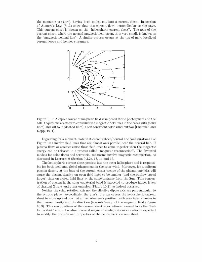
the magnetic pressure), having been pulled out into a current sheet. Inspectionof Ampere’s Law (3.13) show that this current flows perpendicular to the page.This current sheet is known as the “heliospheric current sheet”. The axis of thecurrent sheet, where the normal magnetic field strength is very small, is known asthe “magnetic neutral line”. A similar process occurs at the top of more localizedcoronal loops and helmet streamers.

Figure 10.1: A dipole source of magnetic field is imposed at the photosphere and theMHD equations are used to construct the magnetic field lines in the cases with (solidlines) and without (dashed lines) a self-consistent solar wind outflow [Pneuman andKopp, 1971].

Digressing for a moment, note that current sheet/neutral line configurations likeFigure 10.1 involve field lines that are almost anti-parallel near the neutral line. Ifplasma flows or stresses cause these field lines to come together then the magneticenergy can be released in a process called “magnetic reconnection”. The favouredmodels for solar flares and terrestrial substorms involve magnetic reconnection, asdiscussed in Lectures 9 (Section 9.3.2), 13, 14 and 15.

The heliospheric current sheet persists into the outer heliosphere and is responsi-ble for both local and global phenomena in the solar wind. Moreover, for a uniformplasma density at the base of the corona, easier escape of the plasma particles willcause the plasma density on open field lines to be smaller (and the outflow speedlarger) than on closed field lines at the same distance from the Sun. This concen-tration of plasma in the solar equatorial band is expected to produce higher levelsof thermal X-rays and other emission (Figure 10.2), as indeed observed.

Neither the solar rotation axis nor the effective dipole axis are perpendicular tothe ecliptic plane. Accordingly, the Sun’s rotation causes the heliospheric currentsheet to move up and down at a fixed observer’s position, with associated changes inthe plasma density and the direction (towards/away) of the magnetic field (Figure10.3). This wavy pattern of the current sheet is sometimes referred to as the “bal-lerina skirt” effect. Localized coronal magnetic configurations can also be expectedto modify the position and properties of the heliospheric current sheet.

2

Figure 10.2: An artist’s sketch of the plasma structure and magnetic configurationexpected near the solar equator [Hundhausen, 1972].

Figure 10.3: The “ballerina skirt” ripples predicted on the heliospheric current sheet[Dryer, 1998].

3

10.2 Correlations between coronal and solar wind

properties

X-ray pictures of the Sun from SMM (Solar Maximum Mission), Yohkoh and SOHOshow the existence of both large scale (e.g., coronal holes and the equatorial plasmabelt) and small scale (e.g., active regions) structure in the corona. These magneticand plasma structures can be expected to have counterparts in the solar wind, asthey indeed do.

Figure 10.4 [Severny et al., 1970; Cravens, 1997] compares the disk-averagedcomponent of the solar magnetic field away from (positive) or toward (negative)the Sun with the corresponding time-lagged and averaged solar wind magnetic field.Three important results are apparent. First, the large scale solar field strength iswell correlated with the solar wind field strength in both direction and (scaled)amplitude. This supports the corona being the source of the solar wind magneticfield. Second, the solar wind field varies at the solar rotation period (approximately27 days). Third, distinct, long-lasting intervals of uniform solar wind field directionexist, called “sectors” (Figure 10.5).

Figure 10.6 shows that these magnetic properties are also associated with thesolar wind speed and detailed plasma structures in the corona [e.g., Hundhausen,1972]. Each pair of figures is for a given Carrington rotation (or rotation of the Sun).The lefthand figures show contours of the the coronal X-ray brightness overlaid withthe direction of the photospheric magnetic field outward from or inward to the Sun(+ or -, respectively). Note the primarily equatorial band of intense X-ray emission,as expected from Figure 10.2, and the wavy nature of the current sheet. Positivefield directions lie primarily northward of the equatorial band. The righthand figuresshow time variations in the speed of the solar wind measured in situ at 1 AU.

A number of important results are apparent in Figure 10.6. First, major varia-tions exist in the speed of the solar wind, organised into so-called “fast” and “slowstreams”. Second, fast solar wind streams are associated with times when theEarth is at latitudes poleward of the heliospheric current sheet. These are timeswhen a coronal hole has moved to low heliolatitudes. Third, a given stream car-ries a magnetic field with the polarity (outward or inward) corresponding to thefield orientation of the coronal source region. Fourth, these associations betweenthe coronal and solar wind magnetic field and the solar wind speed are repeatablefrom solar rotation to solar rotation, albeit with variations on several timescales.These variations include small changes due to localized, small-scale and fast timescale coronal structures, while there are also changes associated with large scaleevolution of the corona itself. The overall conclusion here is that fast solar windstreams are associated with coronal holes and open field regions of the corona whileslow streams come from the closed field regions primarily concentrated near theequatorial (or streamer) belt.

The Ulysses spacecraft recently finished its second set of passes over the Sun’snorth and south poles in a polar orbit. Its results allow direct testing of the aboveinterpretations (and investigation of changes with the solar cycle). Figure 10.7shows the solar wind speed, magnetic polarity, and coronal brightness as a functionof time and heliolatitude [McComas et al., 1998]. Clearly, the polar regions docorrespond to high solar wind speed and low density while the equatorial regionscorrespond to slow, relatively dense solar wind speed. Moreover, regions with fastand slow streams correspond to relatively low heliolatitudes where slow streams canleave closed field regions. Finally, the magnetic field shows the expected change inpolarity expected at the heliospheric current sheet.

Two final remarks concerning fast and slow solar wind streams. First, the num-ber and significance of fast and slow solar wind streams varies with the solar cycle:

4

Figure 10.4: The time-averaged away/toward the Sun (positive/negative) compo-nents of the magnetic field in the solar wind (solid lines) are compared with thedisk-averaged away/toward component of the photospheric magnetic field (dashedlines) [Severney et al., 1970].

Figure 10.5: Illustration of sectors of magnetic field lines with different polarities[Cravens, 1997].

5

Figure 10.6: The lefthand figures show contours of the X-ray brightness of the coronaand the sense of the vertical component of the coronal magnetic field direction. Therighthand figures show the solar wind speed and the polarity of the radial componentof the solar wind magnetic field. Adapted from Hundhausen [1972].

6

Figure 10.7: Colour illustration of the solar wind speed and the sense of the mag-netic field’s radial component observed as a function of heliolatitude by the Ulyssesspacecraft [McComas et al., 1998].

more long-lived fast streams are present during the declining phase of the solar cycle(e.g., near solar minimum as sunspots move towards the equator) as coronal holesexpand in size. Second, numerous other plasma properties depend on whether thestream is fast or slow, including the temperature and detailed composition of theplasma and the plasma waves present.

10.3 Co-rotating Interaction Regions: interactions

between fast and slow streams

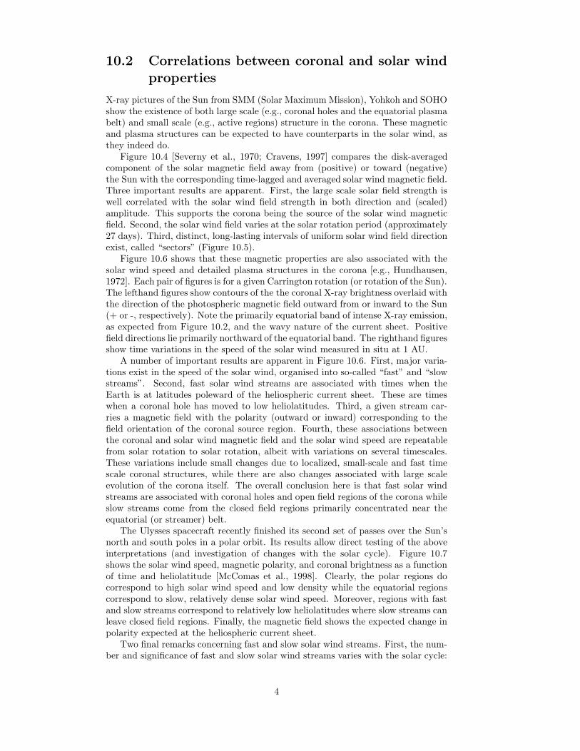
The previous section showed that a fixed observer relatively close to the solar equa-torial plane will observe successive fast and slow solar wind streams during muchof the solar cycle. What interactions are there between these streams? Obviously,there must be interactions because plasma from the fast stream will catch up withand overtake plasma from the slow stream. Figure 10.8 [Hundhausen, 1972] showsthe qualitative predictions of this scenario: formation of a compression region inthe rear of the slow stream, the likely formation of a shock emanating from thecompression region (most likely two, as discussed below), and a rarefaction regionat the rear of the fast steam, all with characteristic variations in the plasma andfield variables. Intuitively it can be seen that these interaction regions will havespiral shapes that may wrap multiple times around the Sun. These regions arecalled “co-rotating interaction regions” or CIRs since they corotate with the Sun.

Co-rotating interaction regions are not always bounded by shocks. The reasonis that shock formation occurs due to the nonlinear steepening of waves, therebyrequiring several nonlinear steepening times to elapse before a shock is formed. Sincemost CIRs do not have shocks at 1 AU but have steepened into shocks by 2 AU,

7

Figure 10.8: Schematic illustration of a fast stream interacting with a slow stream[Hundhausen, 1972].

empirically the nonlinear steepening time must be of order 4 days. (Exercise: why?)One reason why two shocks are eventually formed at a CIR is due to symmetry aboutthe pressure enhancement caused by compression and entraining of the slow windahead of the fast stream (Figure 10.9 [Gosling, 1996]): shocks are driven away fromthe pressure increase in both directions, resulting in a so-called “Forward-Reverseshock pair” in which the forward shock propagates away from the Sun while thereverse shock propagates towards the Sun but is carried out with the solar windflow.

Figure 10.10 [Hundhausen, 1973; Gosling, 1996] displays the results of 1-D MHDsimulations of this process. Note the formation of a pressure increase which drivesforward and reverse shocks with the formation of a characteristic two step increasein the flow speed with a subsequent slow fall-off to the slow speed (in the rarefactionregion). At first sight this two-step profile is inconsistent with both the forward andreverse shock being fast mode shocks. However, this is a reference frame effect: inthe frame of the reverse shock the upstream speed (undisturbed fast stream at latertimes) is greater than the downstream speed (earlier times). In fact, the Rankine-Hugoniot conditions for mass flux across the shock in the shock frame (equation5.17) can be used with the observed upstream and downstream flow speeds tocalculate the shock speed Ush; i.e.,

vup

obs− Ush

vdownobs − Ush

=ndown

nup

. (10.1)

It is emphasized that the reverse shocks are still convected outwards from the Sun,despite attempting to propagate Sunwards.

Figure 10.11 [Smith, 1985] shows the observed evolution of a CIR from 1 AUto 4.2 AU. Note the evidence for magnetic field and plasma compression at 1 AU(lower panels), but an absence of shocks there, which had evolved to a good exampleof a forward-reverse shock pair and CIR by 4.2 AU (upper panels). As the shocksconvect out, however, the forward and reverse shocks move apart and weaken (dueto energy losses associated with heating, compressing, and changing the velocity ofthe downstream plasma). Eventually the forward and reverse shocks from neigh-bouring CIRs cross one another, tending to smooth out the plasma again (However,

8

Figure 10.9: Superposed-epoch analysis of the plasma parameters for CIRs [Goslinget al., 1996]. Note the well defined pressure pulse and compression region in themodified portion of the slow stream.

shock weakening prevents this.). These and similar events can be compared withthe results of MHD simulations: Figure 10.12 [Gosling et al., 1976; Pizzo, 1985]illustrates the very good agreement between observation and theory available usingonly MHD.

Figure 10.13 illustrates the winding up of CIRs (and the Archimedean spiral) atlarge heliocentric distances, where they are clearly likely to have important effectson the plasma. The shock waves and associated structures of CIRs are important innumerous ancillary ways in the solar wind. For instance, CIRs dissipate the energyin fast streams by slowing and heating the plasma, while the magnetic compressionregions and turbulence associated with shocks can scatter cosmic rays. Moreover,particles can be accelerated at the CIR shocks. The shocks and most of the plasmastructure of CIRs are merged together and primarily smoothed out beyond about20 AU. Only the magnetic compression regions tend to persist into the outer helio-sphere beyond 20 AU. These effects are discussed more in Lectures 11 and 20.

10.4 Travelling interplanetary shocks and CMEs

Co-rotating interaction regions and their associated shocks are not the only transientphenomena in the solar wind. Data from the LASCO coronagraph on SOHO makesit clear that many transient releases of matter occur from the Sun, some but notall in association with solar flares. Historically the primary evidence for shocks inthe corona and solar wind came from type II solar radio bursts (whose drift speedsappeared small enough to be associated with a shock moving at the Alfven or fastmode speeds) and from the “Sudden Storm Commencement (SSC)” component

9

Figure 10.10: Evolution towards a CIR state of a high temperature region imposedat the inner boundary of the solar wind [Hundhausen, 1973]. Note the developmentof shocks, a pressure pulse, and the characteristic two-step increase and decay ofthe solar wind speed.

10

Figure 10.11: Figure from Smith [1985] described in the text.

11

Figure 10.12: The top panel shows time profiles of the solar wind speed observedby IMP 7 near 1 AU and by Pioneer 10 near 4.5 AU. The bottom panel comparesthe solar wind speeds measured by Pioneer 10 with those predicted by a 1-D MHDcode using the IMP 7 data as input. Very good agreement is evident [Gosling etal., 1976].

12

Figure 10.13: MHD simulation of (1) high speed streams which cause the develop-ment of CIR structure and (2) the propagation of transient shocks which also modifythe CIR structure (bottom two panels particularly) [Akasofu and Hakamada, 1983].

13

of geomagnetic activity. Until recently it was thought that some shocks observedin the solar wind were associated with blast waves initiated by flares and otherswere driven ahead of plasma clouds ejected from the Sun (“coronal mass ejectionsor CMEs”). Now, however, the current belief is that all non-CIR interplanetaryshocks are associated with CMEs.

The basic situation is illustrated in Figure 10.14 [Cravens, 1997]: a dense, fast,magnetized loop or cloud of plasma is ejected from the Sun, moving like a pistoninto the pre-existing solar wind and creating a compression region bounded bya forward shock. The CME/magnetic cloud often has a force-free configuration

Figure 10.14: Schematic of a coronal mass ejection in the form of a magnetic cloud[Cravens, 1997] with a shock.

and may remain magnetically connected to the Sun even beyond 1 AU; its plasmacomposition and characteristics are often very different from the pre-existing solarwind. Figure 10.15 shows the plasma and magnetic field data for one CME eventobserved near 1 AU. Note the forward shock, the compression of the plasma densityand magnetic field, and the slow rotation of the magnetic field vector inside themagnetic cloud itself (this is a characteristic of a force-free field configuration).

Arguing by analogy with the two shocks associated with the pressure pulsein CIRs, one might expect that CMEs would also drive a reverse shock, at leastbeyond 1 AU. Figure 10.16 shows that this is the case [Gosling, 1996]. Similar toCIR shocks, travelling interplanetary shocks also accelerate particles and generateenhanced plasma waves and radio emissions.

Travelling interplanetary shocks and CME’s affect Earth’s “space weather” en-vironment in a number of ways. First, the change in magnetic field across the shockcauses a time-varying EMF which can overload transformers etc. on communica-tion cables and power grids. Second, the large plasma pressure of the CME andcompression region can significantly move the bow shock and magnetosphere Earth-ward, leading to major currents that can couple to the ionosphere, the ring current,and to terrestrial cables. Third, the shock can inject large numbers of energeticparticles into Earth’s inner magnetosphere, worsening the radiation environmentfor spacecraft and increasing the ring current. These effects will be discussed morein Lecture 15.

14

Figure 10.15: Plasma parameters of a CME and associated shock observed near 1AU [Gosling, 1996].

15

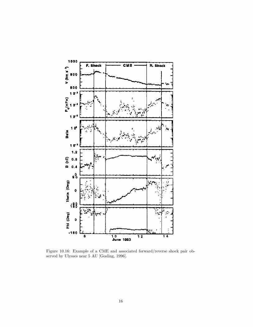
Figure 10.16: Example of a CME and associated forward/reverse shock pair ob-served by Ulysses near 5 AU [Gosling, 1996].

16

10.5 References

• Akasofu, S.-I., and K. Hakamada, Solar wind disturbances in the outer helio-sphere caused by successive solar flares from the same active region, in Solar

Wind 5, NASA Conf. Publ. CP2280, 475, 1983.

• Cravens, T., Introduction to Solar System Plasma Physics, Cambridge, 1997.

• Dryer, M., Solar wind and heliosphere, in The Solar Wind and the Earth, Eds.S.-I. Akasofu and Y. Kamide, D. Reidel, 21, 1987.

• Gosling, J.T., A.J. Hundhausen, and S.J. Bame, Solar wind stream evolutionat large heliocentric distances: Experimental demonstration and the test of amodel, J. Geophys. Res, 81, 2111, 1976.

• Gosling, J.T., Corotating and transient solar wind flows in three dimensions,Ann. Rev. Astron. Astrophys., 34, 35, 1996.

• Hundhausen, A.J., Coronal Expansion and Solar Wind, Springer-Verlag, 1972.

• Hundhausen, A.J., Nonlinear model of high-speed solar wind streams, J. Geo-

phys. Res., 78, 1528, 1973.

• McComas, D.J., et al., Ulysses’ return to the slow solar wind, Geophys.

Res. Lett., 25, 1, 1998.

• Pneuman, G.W., and R.A. Kopp, Solar Phys., 18, 258, 1971.

• Severney, A., J.M. Wilcox, P.H. Scherrer, and D.S. Colburn, Comparison ofthe mean photospheric magnetic field and the interplanetary magnetic field,Solar Phys., 15, 3, 1970.

• Smith, E.J., Interplanetary shock phenomena beyond 1 AU, in Collisionless

Shocks in the Heliosphere: Reviews of Current Research, Eds. B.T. Tsurutaniand R. G. Stone, AGU, 69, 1985.

17