Embed Size (px)
Citation preview
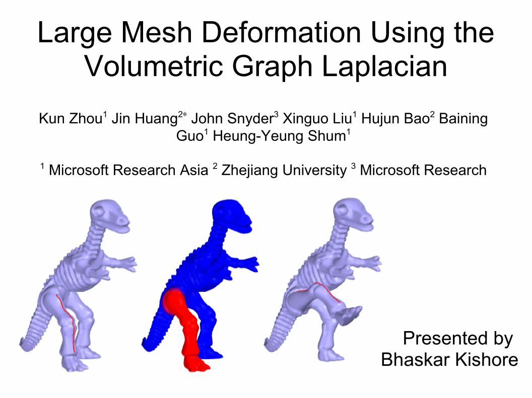
Large Mesh Deformation Using the Volumetric Graph Laplacian
Kun Zhou1 Jin Huang2∗ John Snyder3 Xinguo Liu1 Hujun Bao2 Baining Guo1 Heung-Yeung Shum1
1 Microsoft Research Asia 2 Zhejiang University 3 Microsoft Research
Presented by Bhaskar Kishore

11/21/2007 Bhaskar Kishore 2
Outline
● Introduction● Related Work● Deformation on Volumetric Graphs● Deformation from 2D curves● Results● Conclusions

11/21/2007 Bhaskar Kishore 3
Outline
● Introduction● Related Work● Deformation on Volumetric Graphs● Deformation from 2D curves● Results● Conclusions

11/21/2007 Bhaskar Kishore 4
Introduction
● Large deformations are challenging
● Existing techniques often produce implausible results
● Observation– Unnatural volume
changes– Local Self Intersection

11/21/2007 Bhaskar Kishore 5
Introduction
● Volumetric Graph Laplacian– Represent volumetric details as difference between
each point in a 3D volume and the average of its neighboring points in a graph.
– Produces visually pleasing deformation results– Preserves surface details
● VGL can impose volume constraints ● Volumetric constraints are represented by a
quadric energy function

11/21/2007 Bhaskar Kishore 6
Introduction
● Volumetric Graph Laplacian– Represent volumetric details as difference between
each point in a 3D volume and the average of its neighboring points in a graph.
– Produces visually pleasing deformation results– Preserves surface details
● VGL can impose volume constraints ● Volumetric constraints are represented by a
quadric energy function

11/21/2007 Bhaskar Kishore 7
Introduction
● To apply VGL to a triangle mesh– Construct a volumetric graph which includes
● Points on the original mesh● Points derived from a simple lattice lying inside the mesh
– Points are connected by graph edges which are a superset of the edges of the original mesh
● Whats nice is that there is no need for volumetric tessellation.
● Deformations are specified by identifying a limited set of points – say a curve

11/21/2007 Bhaskar Kishore 8
Introduction
● This curve can then be deformed to specify destination
● A quadric energy function is generated– Minimum maps the points to their specified
destination– While preserving surface detail and roughly volume
too

11/21/2007 Bhaskar Kishore 9
Introduction● Contribution
– Demonstrate that problem of large deformation can be effectively solved by volumetric differential operator
● Surface operators can be extended to solids by defining them on tetrahedral mesh
● But that is difficult, constructing the tetrahedral mesh is hard
● Existing packages remesh geometry and change connectivity
– That a volumetric operator can be applied to the easy to build Volumetric graph without meshing int.

11/21/2007 Bhaskar Kishore 10
Outline
● Introduction● Related Work● Deformation on Volumetric Graphs● Deformation from 2D curves● Results● Conclusions

11/21/2007 Bhaskar Kishore 11
Related Work
● Freeform modeling [Botsch Kobbelt 2004]● Curve based FFD [ Sing and Fiume 1998]● Lattice based FFD [ Sederberg and Parry 1986]● Displacement volumes [Botsch and Kobbelt
2003]● Poisson meshes [Yu et al 2004]

11/21/2007 Bhaskar Kishore 12
Outline
● Introduction● Related Work● Deformation on Volumetric Graphs● Deformation from 2D curves● Results● Conclusions
11/21/2007 Bhaskar Kishore 13
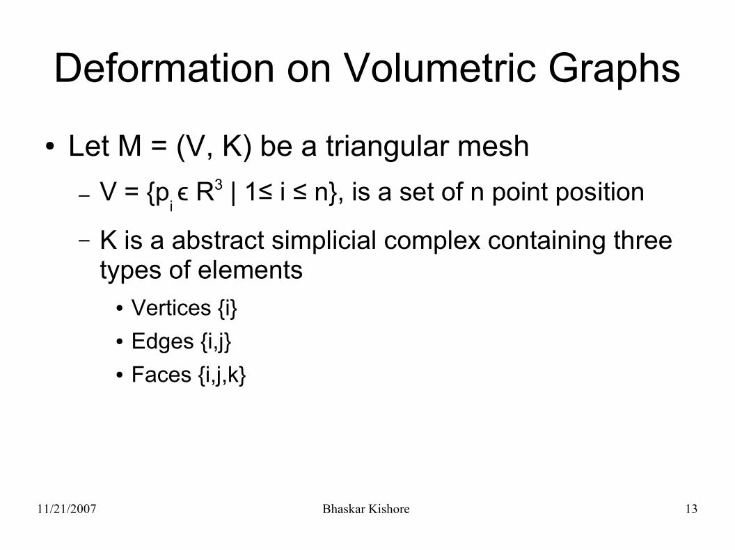
Deformation on Volumetric Graphs
● Let M = (V, K) be a triangular mesh– V = {p
i ϵ R3 | 1≤ i ≤ n}, is a set of n point position
– K is a abstract simplicial complex containing three types of elements
● Vertices {i}● Edges {i,j}● Faces {i,j,k}
11/21/2007 Bhaskar Kishore 14
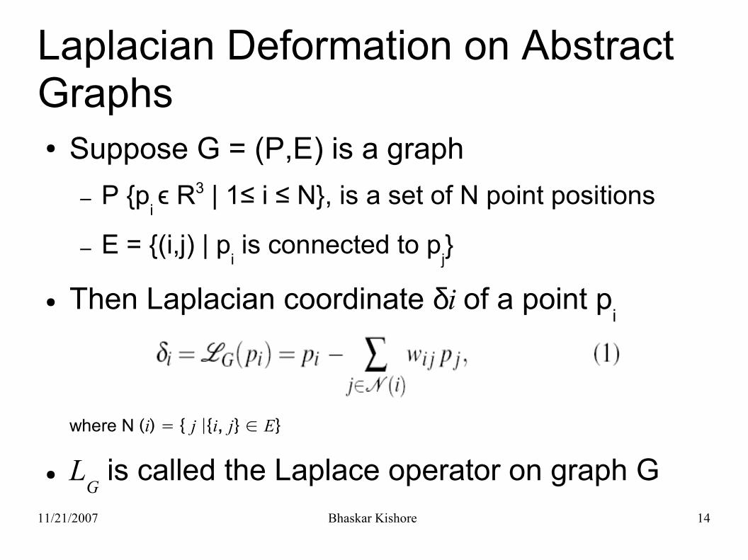
Laplacian Deformation on Abstract Graphs● Suppose G = (P,E) is a graph
– P {pi ϵ R3 | 1≤ i ≤ N}, is a set of N point positions
– E = {(i,j) | pi is connected to p
j}
● Then Laplacian coordinate δi of a point pi
where N (i) = { j |{i, j} ∈ E}
● LG is called the Laplace operator on graph G

11/21/2007 Bhaskar Kishore 15
Laplacian Deformation on Abstract Graphs● To control the deformation
– User inputs deformed positions qi, i ∈ { 1, ..., m} for
a subset of the N mesh vertices– Compute a new (deformed) laplacian coordinate δ'i
for each point i in the graph– Deformed positions of the mesh vertices p'
i is
obtained by solving

11/21/2007 Bhaskar Kishore 16
Laplacian Deformation on Abstract Graphs●
●
● The first term represents preservation of local detail
● The second term constrains the position of those vertices directly specified by the user
● Alpha is used to balance these two objectives

11/21/2007 Bhaskar Kishore 17
Laplacian Deformation on Abstract Graphs● Deformed Laplacian coordinates are computed
viaδ ′
i = T
i δ
i
● δi is the Laplacian in rest pose
● δ ′i is the Laplacian in the deformed pose
● Ti is restricted to rotation and isotropic scale
● Local transforms are propagated from the deformed region to the entire mesh

11/21/2007 Bhaskar Kishore 18
Constructing a Volumetric Graph
● Build two graphs, Gin and G
out
● Gin prevents large volume changes
● Gout
prevents local self-intersection
● Gin can obtained by tetrahedralizing the interior
– Difficult to implement – Computationally expensive– Produces poorly shaped tetrahedra for complex
models

11/21/2007 Bhaskar Kishore 19
Constructing a Volumetric Graph
● Build two graphs, Gin and G
out
● Gin prevents large volume changes
● Gout
prevents local self-intersection
● Gin can obtained by tetrahedralizing the interior
– Difficult to implement – Computationally expensive– Produces poorly shaped tetrahedra for complex
models
11/21/2007 Bhaskar Kishore 20
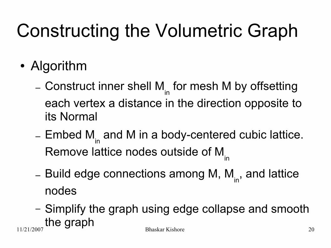
Constructing the Volumetric Graph
● Algorithm– Construct inner shell M
in for mesh M by offsetting
each vertex a distance in the direction opposite to its Normal
– Embed Min and M in a body-centered cubic lattice.
Remove lattice nodes outside of Min
– Build edge connections among M, Min, and lattice
nodes– Simplify the graph using edge collapse and smooth
the graph

11/21/2007 Bhaskar Kishore 21
Constructing the Volumetric Graph
● Construct inner shell Min for mesh M by
offsetting each vertex a distance in the direction opposite to its Normal

11/21/2007 Bhaskar Kishore 22
Constructing the Volumetric Graph
● Embed Min and M in a body-centered cubic
lattice. Remove lattice nodes outside of Min

11/21/2007 Bhaskar Kishore 23
Constructing the Volumetric Graph
● Build edge connections among M, Min, and
lattice nodes

11/21/2007 Bhaskar Kishore 24
Constructing the Volumetric Graph
● Simplify the graph using edge collapse and smooth the graph

11/21/2007 Bhaskar Kishore 25
Constructing the Volumetric Graph
● Min ensures that inner points are inserted even
in thin features that may be missed by lattice sampling.
● Question : how much of a step should one take to construct M
in?
● Use iterative method based on simplification envelopes [Cohen et al. 1996]

11/21/2007 Bhaskar Kishore 26
Constructing the Volumetric Graph
● Min ensures that inner points are inserted even
in thin features that may be missed by lattice sampling.
● Question : how much of a step should one take to construct M
in?
– Use iterative method based on simplification envelopes [Cohen et al. 1996]

11/21/2007 Bhaskar Kishore 27
Constructing the Volumetric Graph
● Use iterative method based on simplification envelopes [Cohen et al. 1996]– At each iteration
● Move each vertex a fraction of the average edge length● Test its adjacent triangles for intersection with each other
and the rest of the model● If no intersections are found, accept step, else reject it● Iterations terminate when all vertices have moved desired
distance or can no longer move

11/21/2007 Bhaskar Kishore 28
Constructing the Volumetric Graph
● Use iterative method based on simplification envelopes [Cohen et al. 1996]– At each iteration
● Move each vertex a fraction of the average edge length● Test its adjacent triangles for intersection with each other
and the rest of the model● If no intersections are found, accept step, else reject it● Iterations terminate when all vertices have moved desired
distance or can no longer move

11/21/2007 Bhaskar Kishore 29
Constructing the Volumetric Graph
● The BCC lattice – Consists of nodes at every point of a Cartesian grid– Additionally there are nodes at cell centers– Node locations may be viewed as belong to two
interlaced grids– This lattice provides desirable rigidity properties as
seen in crystalline structures in nature– Grid interval set to average edge length

11/21/2007 Bhaskar Kishore 30
Constructing the Volumetric Graph● Three types of edge connections for an initial
graph– Each vertex in M is connected to its corresponding
vertex in Min. Shorter diagonal for each prism face is
included as well.– Each inner node of the BCC lattice is connected with its
eight nearest neighbors in the other interlaced grid– Connections are made between Min and nodes of the
BCC lattice.● For each edge in the BCC lattice that intersects Min and
has at least one node inside Min, we connect the BCC
lattice node inside Min to the point in M
in closest to this
intersection

11/21/2007 Bhaskar Kishore 31
Constructing the Volumetric Graph● Three types of edge connections for an initial
graph– Each vertex in M is connected to its corresponding
vertex in Min. Shorter diagonal for each prism face is
included as well.– Each inner node of the BCC lattice is connected with its
eight nearest neighbors in the other interlaced grid– Connections are made between Min and nodes of the
BCC lattice.● For each edge in the BCC lattice that intersects Min and
has at least one node inside Min, we connect the BCC lattice node inside Min to the point in Min closest to this intersection
11/21/2007 Bhaskar Kishore 32
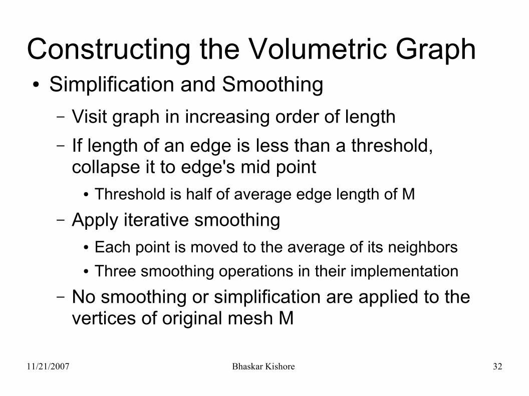
Constructing the Volumetric Graph● Simplification and Smoothing
– Visit graph in increasing order of length– If length of an edge is less than a threshold,
collapse it to edge's mid point● Threshold is half of average edge length of M
– Apply iterative smoothing● Each point is moved to the average of its neighbors● Three smoothing operations in their implementation
– No smoothing or simplification are applied to the vertices of original mesh M

11/21/2007 Bhaskar Kishore 33
Constructing the Volumetric Graph● G
out can be constructed in a similar way to G
in
● Mout
can be obtained by moving a small step in the normal direction.
● Connections for Mout
can be made similar Min
● Intersections between Min and M
out and with M
can occur, especially in meshes containing regions of high curvature. – They claim it does not cause any difficulty in our
interactive system.

11/21/2007 Bhaskar Kishore 34
Deforming the Volumetric Graph
● We modify equation (2) to include volumetric constraints
Where the first n points in graph G belong the mesh M
– G' is a sub-graph of G formed by removing those edges belonging to M
– δ ′i (1 ≤ i ≤ N) in G' are the graph laplcians coordinates in the
deformed frame.– For points in the original mesh M, ε' (1 ≤ i ≤ n) are the mesh
laplacian coordinates in the deformed coordinate frame

11/21/2007 Bhaskar Kishore 35
Deforming the Volumetric Graph
●
– β balances between surface and volumetric detail where β = nβ'/N.
– The n/N factor normalizes the weight so that it is insensitive to the lattice density
– β' = 1 works well– α is not normalized – We want constraint strength to
depend on the number of constrained points relative to the total number of mesh points
● 0.1 < α < 1, default is 0.2

11/21/2007 Bhaskar Kishore 36
Propagation of Local Transforms
● Local Transforms take the Laplacian coordinates in the rest frame to the deformed frame
● Use WIRE deformation method [Singh and Flume]
● Select a sequence of mesh vertices forming a curve
● Deform the curve.

11/21/2007 Bhaskar Kishore 37
Propagation of Local Transforms
● First determine where neighboring graph points deform to, then infers local transforms at the curve points, finally propagate the transforms over the whole mesh
● Begin by finding mesh neighbors of qi and
obtain their deformed positions using WIRE.● Let C(u) and C'(u) be the original curve and the
deformed curves parametrized by arc length u = [0,1]

11/21/2007 Bhaskar Kishore 38
Propagation of Local Transforms
● Given some neighboring point p ϵ R3, let up ϵ
[0,1] be the parameter vale minimizing distnace between p and the curve c(u).
● The deformation mapping p to p' such that C maps to C' is given by
● R is a 3x3 rotation matrix taking the tangent vector t(u) on C and maps it to t'(u) on C' by rotating around t(u)xt'(u)

11/21/2007 Bhaskar Kishore 39
Propagation of Local Transforms
● s(u) is a scale factor– Computed at each curve vertex as the ratio of the
sum of lengths of its adjacent edges in C' over this length in C
– It is then defined continuously over u by liner interpolation
● Above equation gives us deformed coordinates for each point in the curve and its 1 Ring neighborhood

11/21/2007 Bhaskar Kishore 40
Propagation of Local Transforms
● Transformations are propagated from the control curve to all graph points p via a deformation strength field f(p)
● f(p) decays away from the deformation site.– Constant– Linear– Gaussian– Based on shortest edge path from p to the curve

11/21/2007 Bhaskar Kishore 41
Propagation of Local Transforms
● A rotation is defined by– Computing a normal and tangent vector as the
perpendicular projection of one edge vector with this normal
– Normal is computed as a linear combination weighted by face area of face normals around mesh point i
– Rotation is represented as a quaternion● Angle should be less than 180
11/21/2007 Bhaskar Kishore 42
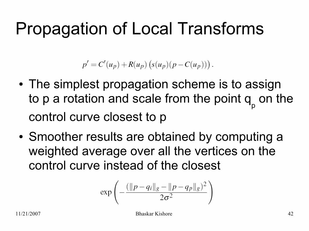
Propagation of Local Transforms
● The simplest propagation scheme is to assign to p a rotation and scale from the point q
p on the
control curve closest to p● Smoother results are obtained by computing a
weighted average over all the vertices on the control curve instead of the closest

11/21/2007 Bhaskar Kishore 43
Propagation of Local Transforms
● Weighting over multiple curves is similar, we accumulate values over multiple curves
● Final transformation matrix is given by

11/21/2007 Bhaskar Kishore 44
Propagation of Local Transforms

11/21/2007 Bhaskar Kishore 45
Weighting Scheme
● They drop uniform weighting in favor of another scheme that provides better results
● For mesh Laplacian Lm, use cotangent weights
● For graph Laplacian, compute weights by solving a quadratic programming problem
11/21/2007 Bhaskar Kishore 46
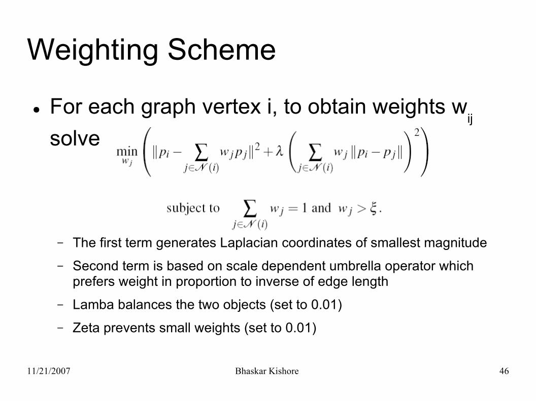
Weighting Scheme
● For each graph vertex i, to obtain weights wij
solve
– The first term generates Laplacian coordinates of smallest magnitude– Second term is based on scale dependent umbrella operator which
prefers weight in proportion to inverse of edge length– Lamba balances the two objects (set to 0.01)– Zeta prevents small weights (set to 0.01)

11/21/2007 Bhaskar Kishore 47
Weighting Scheme

11/21/2007 Bhaskar Kishore 48
Quadric Energy Minimization
● To minimize energy in equation (3) we solve the following equations
– Above equations represent a sparse linear system Ax = b– Matrix A is only dependent on the original graph and A- can be
precomputed using LU decomposition– B depends on current Laplacian coordinates and changes during
interactive deformation

11/21/2007 Bhaskar Kishore 49
Multi resolution Methods
● Solving a the linear system of a large complex model is expensive
● Generate a simplified mesh [Guskov et al. 1999]
● Deform this mesh and then add back the details to obtain high resolution deformed mesh

11/21/2007 Bhaskar Kishore 50
Outline
● Introduction● Related Work● Deformation on Volumetric Graphs● Deformation from 2D curves● Results● Conclusions

11/21/2007 Bhaskar Kishore 51
Deformation from 2D curves
● Method– User defines control curve by selecting sequence
points on the mesh which are connected by the shortest edge path (dijkstra)
– This 3D curve is projected onto one or more planes– Editing is done in these planes– The deformed curve is projected back into 3D,
which then forms the basis of the deformation process
11/21/2007 Bhaskar Kishore 52
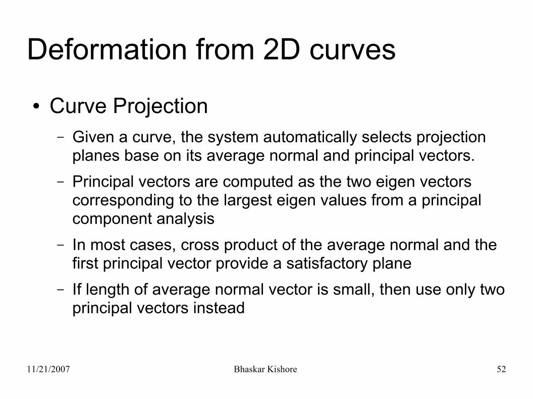
Deformation from 2D curves
● Curve Projection– Given a curve, the system automatically selects projection
planes base on its average normal and principal vectors.– Principal vectors are computed as the two eigen vectors
corresponding to the largest eigen values from a principal component analysis
– In most cases, cross product of the average normal and the first principal vector provide a satisfactory plane
– If length of average normal vector is small, then use only two principal vectors instead

11/21/2007 Bhaskar Kishore 53
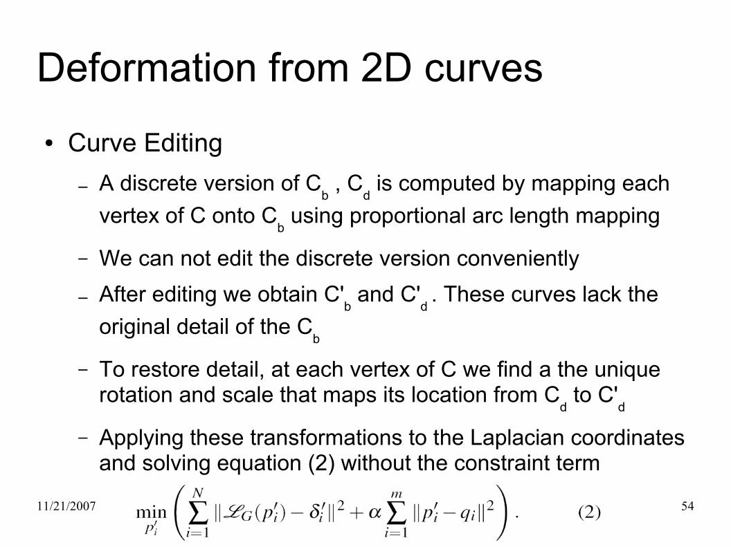
Deformation from 2D curves● Curve Editing
– Projected 2D curves inherit geometric detail from original mesh that complicates editing
– They use an editing method for discrete curves base on Laplacian coordinates
– Laplacian coordinate of a curve vertex is the difference between its position and the average position of its neighbors or a single neighbor in cases of terminal vertices
– Denote the 2D curve to be edited as C
– A cubic B-Spline curve Cb is first computed as a least
squares fit to C. This represents the low frequencies of C
11/21/2007 Bhaskar Kishore 54
Deformation from 2D curves● Curve Editing
– A discrete version of Cb , C
d is computed by mapping each
vertex of C onto Cb using proportional arc length mapping
– We can not edit the discrete version conveniently
– After editing we obtain C'b and C'
d . These curves lack the
original detail of the Cb
– To restore detail, at each vertex of C we find a the unique rotation and scale that maps its location from C
d to C'
d
– Applying these transformations to the Laplacian coordinates and solving equation (2) without the constraint term

11/21/2007 Bhaskar Kishore 55
Deformation from 2D curves● Deformation Re-targeting from 2D Cartoons
– An application of 2D sketch based deformation– Users specify one or more 3D control curves on the mesh along
with their project planes and for each curves a series of 2D curves in the cartoon image sequence that drive its deformation
– It is not necessary to generate a deformation from scratch at every time frame. Users can select a curves in a few key frames of the cartoon
– Automatic interpolation technique based on differential coordinates is used to interpolate between key frame
11/21/2007 Bhaskar Kishore 56
Deformation from 2D curves● Deformation Re-targeting from 2D Cartoons
– Say we have two meshes M and M' at two different key frames– Compute the Laplacian coordinates for each vertex in the two
meshes– A rotation and scale in the local neighborhood of each vertex p is
computed taking the Laplacian coordinates from its location in M to M'
– Denote the transform as Tp. Interpolate T
p over time to transition
from M to M'– 2D cartoon curves are deformed in a single plane, this allows for
extra degrees of freedom if required by the user

11/21/2007 Bhaskar Kishore 57
Deformation from 2D curves● Deformation Re-targeting from 2D Cartoons

11/21/2007 Bhaskar Kishore 58
Deformation from 2D curves● Deformation Re-targeting from 2D Cartoons

11/21/2007 Bhaskar Kishore 59
Outline
● Introduction● Related Work● Deformation on Volumetric Graphs● Deformation from 2D curves● Results● Conclusions

11/21/2007 Bhaskar Kishore 60
Results
● Some stats

11/21/2007 Bhaskar Kishore 61
More results

11/21/2007 Bhaskar Kishore 62
More results

11/21/2007 Bhaskar Kishore 63
Outline
● Introduction● Related Work● Deformation on Volumetric Graphs● Deformation from 2D curves● Results● Conclusions

11/21/2007 Bhaskar Kishore 64
Conclusions
● They proposed a system which would address volumetric changes and local self intersection based on the volumetric graph Laplacian
● The solution avoids the intricacies of solidly meshing complex objects
● Presented a system for retargetting 2D animations to 3D
● Note, that their system does not address global self intersections – those must addressed by the user