Embed Size (px)
Citation preview

Introduction The Model Estimation in Large Dimensions Nonlinear Shrinkage Empirical Study Conclusion
Large Dynamic Covariance Matrices
Robert F. Engle1, Olivier Ledoit2, and Michael Wolf2
1Department of FinanceNew York University
2Department of EconomicsUniversity of Zurich

Introduction The Model Estimation in Large Dimensions Nonlinear Shrinkage Empirical Study Conclusion
Outline
1 Introduction
2 The Model
3 Estimation in Large Dimensions
4 Nonlinear Shrinkage
5 Empirical Study
6 Conclusion

Introduction The Model Estimation in Large Dimensions Nonlinear Shrinkage Empirical Study Conclusion
Outline
1 Introduction
2 The Model
3 Estimation in Large Dimensions
4 Nonlinear Shrinkage
5 Empirical Study
6 Conclusion

Introduction The Model Estimation in Large Dimensions Nonlinear Shrinkage Empirical Study Conclusion
Problem & Aim of the Paper
Problem:
Multivariate GARCH models are popular tools for riskmanagement and portfolio selection
However, the number of assets in the investment universegenerally poses a challenge to such models
In other words, many multivariate GARCH models sufferfrom the curse of dimensionality
Aim of the paper:
Robustify the DCC model of Engle (2002, JBES) againstlarge dimensions
Comparison to all kinds of other multivariate GARCH modelsis left to future research

Introduction The Model Estimation in Large Dimensions Nonlinear Shrinkage Empirical Study Conclusion
Outline
1 Introduction
2 The Model
3 Estimation in Large Dimensions
4 Nonlinear Shrinkage
5 Empirical Study
6 Conclusion

Introduction The Model Estimation in Large Dimensions Nonlinear Shrinkage Empirical Study Conclusion
Notation
Subscripts:
i = 1, . . . ,N indexes assets
t = 1, . . . ,T indexes time
Ingredients:
ri,t: observed return, stacked into rt..= (r1,t, . . . , rN,t)
′
d2i,t
..= Var(ri,t|Ft−1): conditional variance
Dt: diagonal matrix with generic entry di,t
Ht..= Cov(rt|Ft−1): conditional covariance matrix; Diag(Ht) = D2
t
si,t..= ri,t/di,t: devolatilized return, stacked into st
..= (s1,t, . . . , sN,t)′
Rt..= Corr(rt|Ft−1) = Cov(st|Ft−1): conditional correlation matrix
σ2i
..= E(d2i,t
) = Var(ri,t): unconditional variance
C ..= E(Rt) = Corr(rt) = Cov(st): unconditional correlation matrix

Introduction The Model Estimation in Large Dimensions Nonlinear Shrinkage Empirical Study Conclusion
Model Definition
Univariate volatilities governed by a GARCH(1,1) process:
d2i,t = ωi + air
2i,t−1 + bid
2i,t−1
Introduction The Model Estimation in Large Dimensions Nonlinear Shrinkage Empirical Study Conclusion
Model Definition
Univariate volatilities governed by a GARCH(1,1) process:
d2i,t = ωi + air
2i,t−1 + bid
2i,t−1
DCC model of Engle(2002, JBES) with correlation targeting:
Qt = (1 − α − β) C + α st−1s′t−1 + βQt−1 (1)
where Qt is a pseudo conditional correlation matrix.
Conditional correlation and covariance matrices then:
Rt = Diag(Qt)−1/2 Qt Diag(Qt)
−1/2
Ht = DtRtDt
Data generating process:
rt|Ft−1 ∼ N(0,Ht)

Introduction The Model Estimation in Large Dimensions Nonlinear Shrinkage Empirical Study Conclusion
Outline
1 Introduction
2 The Model
3 Estimation in Large Dimensions
4 Nonlinear Shrinkage
5 Empirical Study
6 Conclusion

Introduction The Model Estimation in Large Dimensions Nonlinear Shrinkage Empirical Study Conclusion
Making Estimation Feasible
Estimating the model with a large number of assets is challenging.
Major difficulty:
Inverting the conditional covariance matrix Ht for the likelihood

Introduction The Model Estimation in Large Dimensions Nonlinear Shrinkage Empirical Study Conclusion
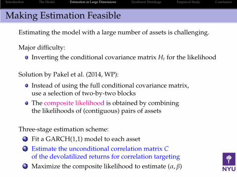
Making Estimation Feasible
Estimating the model with a large number of assets is challenging.
Major difficulty:
Inverting the conditional covariance matrix Ht for the likelihood
Solution by Pakel et al. (2014, WP):
Instead of using the full conditional covariance matrix,use a selection of two-by-two blocks
The composite likelihood is obtained by combiningthe likelihoods of (contiguous) pairs of assets
Introduction The Model Estimation in Large Dimensions Nonlinear Shrinkage Empirical Study Conclusion
Making Estimation Feasible
Estimating the model with a large number of assets is challenging.
Major difficulty:
Inverting the conditional covariance matrix Ht for the likelihood
Solution by Pakel et al. (2014, WP):
Instead of using the full conditional covariance matrix,use a selection of two-by-two blocks
The composite likelihood is obtained by combiningthe likelihoods of (contiguous) pairs of assets
Three-stage estimation scheme:
1 Fit a GARCH(1,1) model to each asset
2 Estimate the unconditional correlation matrix Cof the devolatilized returns for correlation targeting
3 Maximize the composite likelihood to estimate (α, β)

Introduction The Model Estimation in Large Dimensions Nonlinear Shrinkage Empirical Study Conclusion
Outline
1 Introduction
2 The Model
3 Estimation in Large Dimensions
4 Nonlinear Shrinkage
5 Empirical Study
6 Conclusion
Introduction The Model Estimation in Large Dimensions Nonlinear Shrinkage Empirical Study Conclusion
Nonlinear Shrinkage to Counter Large Dimensions
Main contribution:
Improved estimation of the unconditional correlation matrix C,which serves as the correlation target in equation (1)

Introduction The Model Estimation in Large Dimensions Nonlinear Shrinkage Empirical Study Conclusion
Nonlinear Shrinkage to Counter Large Dimensions
Main contribution:
Improved estimation of the unconditional correlation matrix C,which serves as the correlation target in equation (1)
Naıve approach:
Use the sample correlation matrix of the devolatilized returns st
Corresponds to the original proposal of Engle (2002, JBES)
This approach does not work well in large dimensions,and cannot even be used when N > T
Superior approach:
Apply nonlinear shrinkage to the devolatilized returns st
This approach works well in large dimensions, even when N > T

Introduction The Model Estimation in Large Dimensions Nonlinear Shrinkage Empirical Study Conclusion
Nonlinear Shrinkage: Starting Point
Generic setting:
I.i.d. data yt ∈ RN with covariance matrix Σ
Stacked into T ×N matrix Y

Introduction The Model Estimation in Large Dimensions Nonlinear Shrinkage Empirical Study Conclusion
Nonlinear Shrinkage: Starting Point
Generic setting:
I.i.d. data yt ∈ RN with covariance matrix Σ
Stacked into T ×N matrix Y
The sample covariance matrix S admits a spectral decomposition
S = UΛU′
Here:
U is an orthogonal matrix whose columns arethe sample eigenvectors (u1, . . . ,uN)
Λ is a diagonal matrix whose diagonal entries arethe sample eigenvalues (λ1, . . . , λN)
Introduction The Model Estimation in Large Dimensions Nonlinear Shrinkage Empirical Study Conclusion
Nonlinear Shrinkage: Class of Estimators
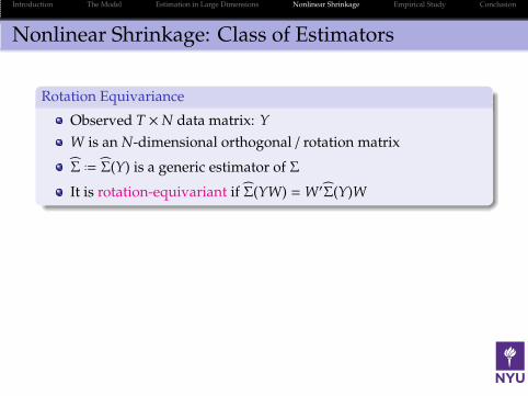
Rotation Equivariance
Observed T ×N data matrix: Y
W is an N-dimensional orthogonal / rotation matrix
Σ ..= Σ(Y) is a generic estimator of Σ
It is rotation-equivariant if Σ(YW) =W′Σ(Y)W

Introduction The Model Estimation in Large Dimensions Nonlinear Shrinkage Empirical Study Conclusion
Nonlinear Shrinkage: Class of Estimators
Rotation Equivariance
Observed T ×N data matrix: Y
W is an N-dimensional orthogonal / rotation matrix
Σ ..= Σ(Y) is a generic estimator of Σ
It is rotation-equivariant if Σ(YW) =W′Σ(Y)W
Without specific knowledge about Σ, rotation equivarianceis a desirable property of an estimator.
We use the following class of rotation-equivariant estimatorsgoing back to Stein (1975, 1986):
Σ ..= UDU′ where D ..= Diag(d1, . . . , dN) is diagonal

Introduction The Model Estimation in Large Dimensions Nonlinear Shrinkage Empirical Study Conclusion
Nonlinear Shrinkage In Action
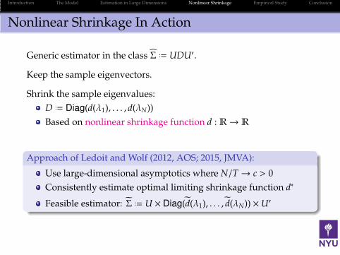
Generic estimator in the class Σ ..= UDU′.
Keep the sample eigenvectors.
Shrink the sample eigenvalues:
D ..= Diag(d(λ1), . . . , d(λN))
Based on nonlinear shrinkage function d : R→ R
Introduction The Model Estimation in Large Dimensions Nonlinear Shrinkage Empirical Study Conclusion
Nonlinear Shrinkage In Action
Generic estimator in the class Σ ..= UDU′.
Keep the sample eigenvectors.
Shrink the sample eigenvalues:
D ..= Diag(d(λ1), . . . , d(λN))
Based on nonlinear shrinkage function d : R→ R
Approach of Ledoit and Wolf (2012, AOS; 2015, JMVA):
Use large-dimensional asymptotics where N/T→ c > 0
Consistently estimate optimal limiting shrinkage function d∗
Feasible estimator: Σ ..= U × Diag(d(λ1), . . . , d(λN)) ×U′
Further Details on Nonlinear Shrinkage
Introduction The Model Estimation in Large Dimensions Nonlinear Shrinkage Empirical Study Conclusion
Proposed Estimation of the DCC Model
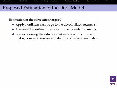
Estimation of the correlation target C:
Apply nonlinear shrinkage to the devolatilized returns st
The resulting estimator is not a proper correlation matrix
Post-processing the estimator takes care of this problem,that is, convert covariance matrix into a correlation matrix
Introduction The Model Estimation in Large Dimensions Nonlinear Shrinkage Empirical Study Conclusion
Proposed Estimation of the DCC Model
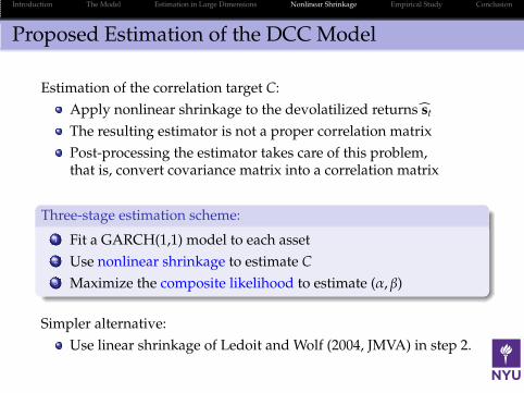
Estimation of the correlation target C:
Apply nonlinear shrinkage to the devolatilized returns st
The resulting estimator is not a proper correlation matrix
Post-processing the estimator takes care of this problem,that is, convert covariance matrix into a correlation matrix
Three-stage estimation scheme:
1 Fit a GARCH(1,1) model to each asset
2 Use nonlinear shrinkage to estimate C
3 Maximize the composite likelihood to estimate (α, β)
Simpler alternative:
Use linear shrinkage of Ledoit and Wolf (2004, JMVA) in step 2.

Introduction The Model Estimation in Large Dimensions Nonlinear Shrinkage Empirical Study Conclusion
Linear Shrinkage
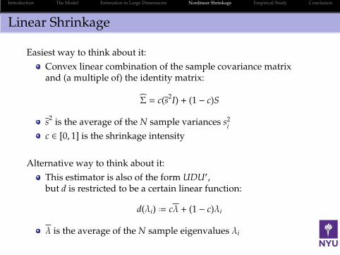
Easiest way to think about it:
Convex linear combination of the sample covariance matrixand (a multiple of) the identity matrix:
Σ = c(s2I) + (1 − c)S
s2
is the average of the N sample variances s2i
c ∈ [0, 1] is the shrinkage intensity
Introduction The Model Estimation in Large Dimensions Nonlinear Shrinkage Empirical Study Conclusion
Linear Shrinkage
Easiest way to think about it:
Convex linear combination of the sample covariance matrixand (a multiple of) the identity matrix:
Σ = c(s2I) + (1 − c)S
s2
is the average of the N sample variances s2i
c ∈ [0, 1] is the shrinkage intensity
Alternative way to think about it:
This estimator is also of the form UDU′,but d is restricted to be a certain linear function:
d(λi) ..= cλ + (1 − c)λi
λ is the average of the N sample eigenvalues λi

Introduction The Model Estimation in Large Dimensions Nonlinear Shrinkage Empirical Study Conclusion
Outline
1 Introduction
2 The Model
3 Estimation in Large Dimensions
4 Nonlinear Shrinkage
5 Empirical Study
6 Conclusion

Introduction The Model Estimation in Large Dimensions Nonlinear Shrinkage Empirical Study Conclusion
Big Picture
Goal:
Examine out-of-sample properties of Markowitz portfoliosvia backtest exercises

Introduction The Model Estimation in Large Dimensions Nonlinear Shrinkage Empirical Study Conclusion
Big Picture
Goal:
Examine out-of-sample properties of Markowitz portfoliosvia backtest exercises
Two applications:
Global minimum variance (GMV) portfolio
Full Markowitz portfolio with a signal

Introduction The Model Estimation in Large Dimensions Nonlinear Shrinkage Empirical Study Conclusion
Big Picture
Goal:
Examine out-of-sample properties of Markowitz portfoliosvia backtest exercises
Two applications:
Global minimum variance (GMV) portfolio
Full Markowitz portfolio with a signal
(Out-of-sample) Performance measures:
Standard deviation
Information ratio

Introduction The Model Estimation in Large Dimensions Nonlinear Shrinkage Empirical Study Conclusion
Data & Portfolio Rules
Data:
Download daily return data from CRSP
Period: 01/01/1980–12/31/2015

Introduction The Model Estimation in Large Dimensions Nonlinear Shrinkage Empirical Study Conclusion
Data & Portfolio Rules
Data:
Download daily return data from CRSP
Period: 01/01/1980–12/31/2015
Updating:
21 consecutive trading days constitute one ‘month’
Update portfolios on ‘monthly’ basis

Introduction The Model Estimation in Large Dimensions Nonlinear Shrinkage Empirical Study Conclusion
Data & Portfolio Rules
Data:
Download daily return data from CRSP
Period: 01/01/1980–12/31/2015
Updating:
21 consecutive trading days constitute one ‘month’
Update portfolios on ‘monthly’ basis
Out-of-sample period:
Start investing on 01/08/1986
This results in 7560 daily returns (over 360 ‘months’)

Introduction The Model Estimation in Large Dimensions Nonlinear Shrinkage Empirical Study Conclusion
Data & Portfolio Rules
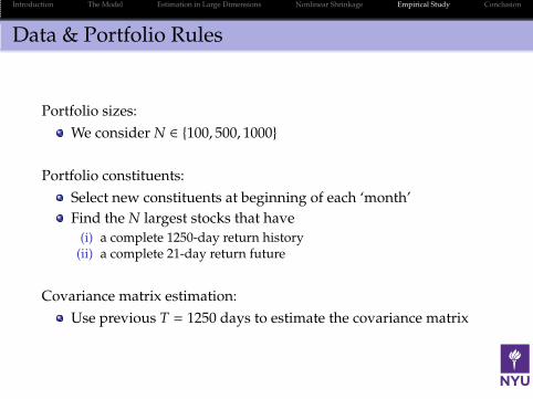
Portfolio sizes:
We consider N ∈ {100, 500, 1000}

Introduction The Model Estimation in Large Dimensions Nonlinear Shrinkage Empirical Study Conclusion
Data & Portfolio Rules
Portfolio sizes:
We consider N ∈ {100, 500, 1000}
Portfolio constituents:
Select new constituents at beginning of each ‘month’
Find the N largest stocks that have
(i) a complete 1250-day return history(ii) a complete 21-day return future
Covariance matrix estimation:
Use previous T = 1250 days to estimate the covariance matrix

Introduction The Model Estimation in Large Dimensions Nonlinear Shrinkage Empirical Study Conclusion
Global Minimum Variance Portfolio
Problem Formulation
minw
w′Htw
subject to w′1 = 1
(where 1 is a conformable vector of ones)

Introduction The Model Estimation in Large Dimensions Nonlinear Shrinkage Empirical Study Conclusion
Global Minimum Variance Portfolio
Problem Formulation
minw
w′Htw
subject to w′1 = 1
(where 1 is a conformable vector of ones)
Analytical Solution
w∗ =H−1
t 1
1′H−1t 1

Introduction The Model Estimation in Large Dimensions Nonlinear Shrinkage Empirical Study Conclusion
Global Minimum Variance Portfolio
Problem Formulation
minw
w′Htw
subject to w′1 = 1
(where 1 is a conformable vector of ones)
Analytical Solution
w∗ =H−1
t 1
1′H−1t 1
Feasible Solution
w ..=H−1
t 1
1′H−1t 1

Introduction The Model Estimation in Large Dimensions Nonlinear Shrinkage Empirical Study Conclusion
Global Mininum Variance Portfolio
Competing portfolios:
1/N: as a simple benchmark
DCC-S: based on the sample correlation matrix
DCC-L: based on linear shrinkage
DCC-NL: based on nonlinear shrinkage
RM-2006: RiskMetrics 2006
Performance measures:
Standard deviation (primary)
Information ratio (secondary)
Assessing statistical significance:
Test for significant difference between DCC-S and DCC-NLuses Ledoit and Wolf (2011, WM)

Introduction The Model Estimation in Large Dimensions Nonlinear Shrinkage Empirical Study Conclusion
Global Mininum Variance Portfolio
Annualized standard deviations:
N 1/N DCC-S DCC-L DCC-NL RM-2006100 21.56 13.36 13.33 13.17∗∗∗ 14.69500 19.53 10.57 10.40 9.64∗∗∗ 12.60
1000 19.04 10.59 9.14 8.02∗∗∗ 14.86
Remarks:
In each row, the best number appears in blue
Stars indicate significant outperformance (DCC-NL vs. DCC-S)

Introduction The Model Estimation in Large Dimensions Nonlinear Shrinkage Empirical Study Conclusion
Global Mininum Variance Portfolio
Annualized information ratios:
N 1/N DCC-S DCC-L DCC-NL RM-2006100 0.56 0.74 0.74 0.76 0.57500 0.69 1.32 1.33 1.39 0.891000 0.75 1.11 1.33 1.52 0.77
Remarks:
In each row, the best number appears in blue

Introduction The Model Estimation in Large Dimensions Nonlinear Shrinkage Empirical Study Conclusion
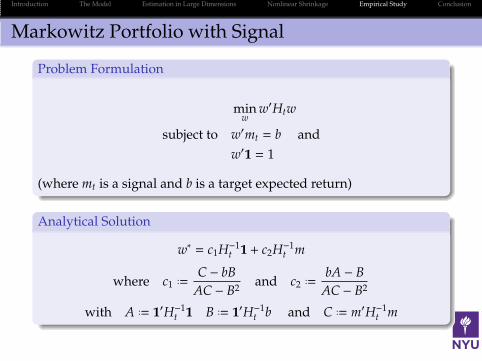
Markowitz Portfolio with Signal
Problem Formulation
minw
w′Htw
subject to w′mt = b and
w′1 = 1
(where mt is a signal and b is a target expected return)
Introduction The Model Estimation in Large Dimensions Nonlinear Shrinkage Empirical Study Conclusion
Markowitz Portfolio with Signal
Problem Formulation
minw
w′Htw
subject to w′mt = b and
w′1 = 1
(where mt is a signal and b is a target expected return)
Analytical Solution
w∗ = c1H−1t 1 + c2H−1
t m
where c1..=
C − bB
AC − B2and c2
..=bA − B
AC − B2
with A ..= 1′H−1t 1 B ..= 1′H−1
t b and C ..= m′H−1t m
Feasible Solution w replaces Ht with an estimator Ht.

Introduction The Model Estimation in Large Dimensions Nonlinear Shrinkage Empirical Study Conclusion
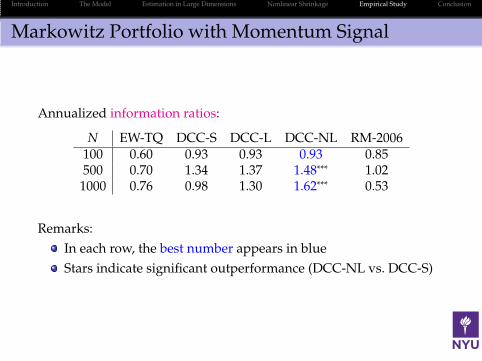
Markowitz Portfolio with Momentum Signal
For simplicity and reproducibility, we use momentum as the signal.

Introduction The Model Estimation in Large Dimensions Nonlinear Shrinkage Empirical Study Conclusion
Markowitz Portfolio with Momentum Signal
For simplicity and reproducibility, we use momentum as the signal.
Competing portfolios:
EW-TQ: equal-weighted portfolio of top-quintiles stocks=⇒ yields target expected return b for other portfolios
DCC-S: based on the sample correlation matrix
DCC-L: based on linear shrinkage
DCC-NL: based on nonlinear shrinkage
RM-2006: RiskMetrics 2006
Performance measure:
Standard deviation (secondary)
Information ratio (primary)
Assessing statistical significance:
Test for significant difference between DCC-S and DCC-NLuses Ledoit and Wolf (2008, JEF)

Introduction The Model Estimation in Large Dimensions Nonlinear Shrinkage Empirical Study Conclusion
Markowitz Portfolio with Momentum Signal
Annualized standard deviations:
N EW-TQ DCC-S DCC-L DCC-NL RM-2006100 28.43 17.05 17.03 16.90∗∗∗ 18.87500 24.42 12.36 12.16 11.31∗∗∗ 16.14
1000 22.89 13.07 10.76 9.20∗∗∗ 29.29
Remarks:
In each row, the best number appears in blue
Stars indicate significant outperformance (DCC-NL vs. DCC-S)
Introduction The Model Estimation in Large Dimensions Nonlinear Shrinkage Empirical Study Conclusion
Markowitz Portfolio with Momentum Signal
Annualized information ratios:
N EW-TQ DCC-S DCC-L DCC-NL RM-2006100 0.60 0.93 0.93 0.93 0.85500 0.70 1.34 1.37 1.48∗∗∗ 1.02
1000 0.76 0.98 1.30 1.62∗∗∗ 0.53
Remarks:
In each row, the best number appears in blue
Stars indicate significant outperformance (DCC-NL vs. DCC-S)

Introduction The Model Estimation in Large Dimensions Nonlinear Shrinkage Empirical Study Conclusion
Outline
1 Introduction
2 The Model
3 Estimation in Large Dimensions
4 Nonlinear Shrinkage
5 Empirical Study
6 Conclusion

Introduction The Model Estimation in Large Dimensions Nonlinear Shrinkage Empirical Study Conclusion
Conclusion
Multivariate GARCH models are popular tools for risk managementand portfolio selection, but are often challenged in large dimensions.

Introduction The Model Estimation in Large Dimensions Nonlinear Shrinkage Empirical Study Conclusion
Conclusion
Multivariate GARCH models are popular tools for risk managementand portfolio selection, but are often challenged in large dimensions.
Two keys for making DCC model robust against large dimensions:
1 Composite likelihood makes estimation feasible
2 Nonlinear shrinkage estimation of the correlation targetingmatrix ensures good performance
Resulting DCC-NL model:
Outperforms the basic DCC-S model by a wide margin
Should become the new DCC standard
Remark:
Nonlinear shrinkage can also help in robustifying othermultivariate GARCH models against large dimensions
A short description for the scalar BEKK model is in the paper

Engle, R. F. (2002). Dynamic conditional correlation: A simple class ofmultivariate generalized autoregressive conditional heteroskedasticitymodels. Journal of Business & Economic Statistics, 20(3):339–350.
Ledoit, O. and Wolf, M. (2008). Robust performance hypothesis testing withthe Sharpe ratio. Journal of Empirical Finance, 15:850–859.
Ledoit, O. and Wolf, M. (2011). Robust performance hypothesis testing withthe variance. Wilmott Magazine, September:86–89.
Ledoit, O. and Wolf, M. (2012). Nonlinear shrinkage estimation oflarge-dimensional covariance matrices. Annals of Statistics, 40(2):1024–1060.
Ledoit, O. and Wolf, M. (2015). Spectrum estimation: a unified framework forcovariance matrix estimation and PCA in large dimensions. Journal ofMultivariate Analysis, 139(2):360–384.
Ledoit, O. and Wolf, M. (2017). Nonlinear shrinkage of the covariance matrixfor portfolio selection: Markowitz meets Goldilocks. Review of FinancialStudies. Forthcoming.
Pakel, C., Shephard, N., Sheppard, K., and Engle, R. F. (2014). Fitting vastdimensional time-varying covariance models. Technical report.
Stein, C. (1975). Estimation of a covariance matrix. Rietz lecture, 39th AnnualMeeting IMS. Atlanta, Georgia.
Stein, C. (1986). Lectures on the theory of estimation of many parameters.Journal of Mathematical Sciences, 34(1):1373–1403.

Asymptotic Framework
Let N ..= N(T) and assume N/T→ c > 0, as T→∞.
The following set of assumptions is maintained throughout.
A1 The population covariance matrix ΣT is a nonrandom N-dimensionalpositive definite matrix.
A2 Let XT be an T ×N matrix of real i.i.d. random variables with zero mean,unit variance, and finite twelfth moment. One observes YT
..= XTΣ1/2T
.
A3 Let ((τT,1, . . . , τT,N); (vT,1, . . . , vT,N)) denote the eigenvaluesand eigenvectors of ΣT. The e.d.f. of the population eigenvalues,denoted by HT, converges weakly to some limiting e.d.f. H.
A4 Supp(H), the support of H, is the union of a finite number of closedintervals, bounded away from zero and infinity. Furthermore, thereexists a compact interval in (0,+∞) that contains Supp(HT) for all Tlarge enough.

Ukranian Foundation
The Stieltjes transform of a nondecreasing function G is:
∀z ∈ C+ mG(z) ..=
∫ +∞
−∞
1
λ − zdG(λ)
(It has an explicit inversion formula too.)
Denote the e.d.f. of the sample eigenvalues by FT.
Marcenko and Pastur (1967) showed that FT converges a.s.to some nonrandom limit F at all points of continuity of F.
They also discovered how mF relates to H and c:
∀z ∈ C+ mF(z) =
∫ +∞
−∞
1
τ[1 − c − c z mF(z)
]− z
dH(τ) (2)
This is the celebrated Marcenko-Pastur (MP) equation.

Transatlantic Additions
Moral: knowing H and c, one can ‘solve’ for F.
The particular expression (2) of the MP equation is due to Silverstein (1995).
Silverstein and Choi (1995) showed that
∀λ ∈ R limz∈C+→λ
mF(z) =.. mF(λ) exists
The quantity mF(λ) will be of crucial importance.
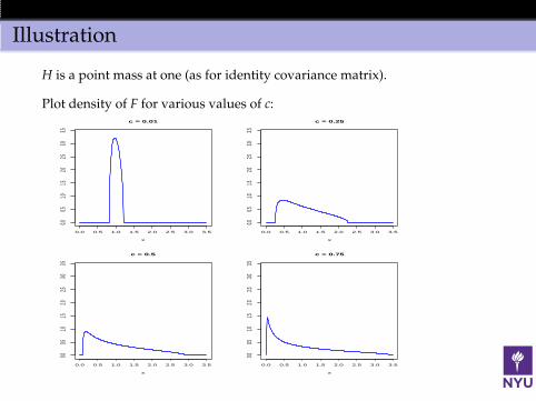
Illustration
H is a point mass at one (as for identity covariance matrix).
Plot density of F for various values of c:
0.0 0.5 1.0 1.5 2.0 2.5 3.0 3.5
0.00.5
1.01.5
2.02.5
3.03.5
c = 0.01
x
0.0 0.5 1.0 1.5 2.0 2.5 3.0 3.5
0.00.5
1.01.5
2.02.5
3.03.5
c = 0.25
x
0.0 0.5 1.0 1.5 2.0 2.5 3.0 3.5
0.00.5
1.01.5
2.02.5
3.03.5
c = 0.5
x
0.0 0.5 1.0 1.5 2.0 2.5 3.0 3.5
0.00.5
1.01.5
2.02.5
3.03.5
c = 0.75
x

Optimization Problem
(Standardized) Frobenius norm:
||A|| ..=√
Tr(AA′)/r for any matrix A of dimension r ×m

Optimization Problem
(Standardized) Frobenius norm:
||A|| ..=√
Tr(AA′)/r for any matrix A of dimension r ×m
Loss function:
L(UTDTUT,ΣT) ..= ||UTDTUT − ΣT ||2

Optimization Problem
(Standardized) Frobenius norm:
||A|| ..=√
Tr(AA′)/r for any matrix A of dimension r ×m
Loss function:
L(UTDTUT,ΣT) ..= ||UTDTUT − ΣT ||2
Line of attack:
It turns out that there is nonstochastic limit of the loss function,which involves the shrinkage function d
We minimize the limiting expression with respect to d

Nonlinear Shrinkage Estimator
We illustrate the methodology for the case c ≤ 1.

Nonlinear Shrinkage Estimator
We illustrate the methodology for the case c ≤ 1.
Optimal limiting shrinkage function
d∗(λ) ..=λ
∣∣∣1 − c − cλ mF(λ)∣∣∣2

Nonlinear Shrinkage Estimator
We illustrate the methodology for the case c ≤ 1.
Optimal limiting shrinkage function
d∗(λ) ..=λ
∣∣∣1 − c − cλ mF(λ)∣∣∣2
A feasible estimator is obtained by:
Replacing c with N/T
Consistently estimating mF, which is achieved by consistentlyestimating H and putting it in the MP equation together with N/T
Resulting estimator: ΣT..= UT × Diag(dT(λT,1), . . . , dT(λT,N)) ×U′
T
The methodology can be extended to the case c > 1.
Back to Main Talk