Embed Size (px)
Citation preview

Landscape change in southwest China’s Himalayan Mountains:
Implications for old-growth forests, alpine meadows, and avian diversity
By
Jodi S. Brandt
A dissertation submitted in partial fulfillment of
the requirements for the degree of
Doctor of Philosophy
(Forest and Wildlife Ecology)
At the
UNIVERSITY OF WISCONSIN-MADISON
2012
Date of final oral examination: 5/15/2012
The dissertation is approved by the following members of the Final Oral Committee:
Volker C. Radeloff, Professor, Forest and Wildlife Ecology
Mutlu Ozdogan, Assistant Professor, Forest and Wildlife Ecology
Anna Pidgeon, Assistant Professor, Forest and Wildlife Ecology
Philip Townsend, Professor, Forest and Wildlife Ecology
A-Xing Zhu, Professor, Department of Geography

i
Abstract
Land use and land cover change (LULCC) is the main cause of biodiversity declines
worldwide. Many of the remaining high-diversity ecosystems are located in developing
countries, which are undergoing rapid development and population growth. High biodiversity
often occurs in the same areas where people dwell, and our understanding of how to balance
livelihoods and conservation is limited. Population growth, economic development, conservation
policies and climate change interact at multiple spatial and temporal scales to form complex
LULCC dynamics, with unexpected consequences for biodiversity.
My overarching goal was to identify effective conservation strategies in developing
countries. To this end, I focused on a case study in northwest (NW) Yunnan, a biodiversity
hotspot in the remote Chinese Himalayas. NW Yunnan is subject to many forces of change
acting at multiple scales, including environmental protection policies, rapid economic
development, indigenous land use practices, and climate change. I used satellite imagery to
investigate the patterns and drivers of land cover change from 1974 to 2009, and I integrated
ecological field data to understand how the observed changes influenced biodiversity.
My results showed that the two highest-diversity ecosystems in NW Yunnan – old-growth
forest and alpine meadows – underwent rapid land cover changes that have negative implications
for biodiversity. First, I studied change in forest ecosystems, which cover approximately 65% of
NW Yunnan. I found that after the landmark logging ban in 1998, overall forest cover increased
from 62% in 1990 to 64% in 2009. However, clearing of high-diversity old-growth forest
accelerated, from approximately 1100 hectares/year before the logging ban (1990 to 1999), to
1550 hectares/year after the logging ban (1999 to 2009). Paradoxically, old-growth forest

ii
clearing accelerated most rapidly where ecotourism was most prominent. Increasing forest cover
represented mainly non-pine scrub forests, which were not on a trajectory towards becoming
high-diversity forest stands.
Second, I analyzed change in alpine meadows, which have exceptionally high species
richness, beta diversity, and endemism. I found that, between 1990 and 2009, at least 39% of
alpine meadows converted to woody shrubs. The patterns of change suggest that a catastrophic
regime shift is occurring, driven by feedback mechanisms involving climate change,
environmental policy that prohibited intentional burning and economic development that
increased grazing pressure. Shrub expansion threatens alpine meadow biodiversity and local
Tibetan yak herder livelihoods, and more generally, these trends serve as a warning sign for the
greater Himalayan region where similar vegetation changes could greatly affect biodiversity,
livelihoods, hydrology, and climate.
Finally, I studied the role of Tibetan sacred forests for avian biodiversity. I collected breeding
bird and habitat data in six Tibetan sacred forest sites and their surrounding matrix. I found that
sacred forests protected old-growth forest ecosystems, supported a significantly different bird
community than the surrounding matrix, and had higher bird species richness at multiple scales.
While bird community composition was primarily driven by the vertical structure of the
vegetation, plots with the largest trees (height or diameter) and bamboo groves had the highest
bird diversity and abundance, indicating the importance of protecting old-growth forest
ecosystems for Himalayan forest birds.
In general, my dissertation shows that complex interactions between environmental policy,
economic development strategy, and climate change in tightly coupled human-nature systems

iii
can lead to unexpected trajectories of land cover change. Satellite imagery, when paired with
ecological field data, can measure these broad-scale changes and their implications for
biodiversity, thereby informing policy and management in a timely manner.

iv
Acknowledgements
There is a lot of “I” in this document, but this dissertation was actually a group effort. I am
indebted to all of the people in Madison, Wisconsin and Yunnan, China who contributed to this
endeavor. I will always be grateful to my advisor, Volker Radeloff, for being so generous with
his compliments and kind with his critiques. I thank my committee for their expert and
enthusiastic guidance: I especially appreciate Phil Townsend for setting me off on my scientific
path, A-xing Zhu for teaching me how to make a proper Chinese toast, Mutlu Ozdogan for his
razor sharp mind, and Anna Pidgeon for blazing a trail through the forest of men. Tobias
Kuemmerle and Eric Wood deserve special thanks for their patient mentorship. Teri Allendorf
and the IGERT executive committee provided unflagging logistical and financial support for my
research. I thank Michelle Haynes for ushering me through the maze, and Fang Zhendong and
Han Lian-xian for sharing their expertise in the field. I also thank Shelley Schmidt for the daily
reality check and Dave “no beer left behind” Helmers for technical assistance. I am grateful to all
of the members of the SILVIS lab for their friendship.
A special shout-out goes to those who put up with me these past 5 years even though it’s not
their job. Mom, Dad, Booger and Craigy – thank you for thinking I’m great no matter what.
Lady Sassafras, thanks for going to the police station and reclaiming all my stolen stuff. Thanks
to Healthy-and-Clean for the pickled vegetables, to Jane for teaching me the difference between
a duck and a goose, and to Dr. Big Logs for the qi. Thanks to Clayton for the Singani and Cindee
for the tabouli. And Mary and Kiera, thanks a million for pulling me out of that campfire.
Finally, I am especially grateful to have known Josh Posner. He was an inspiring example, in
health and in illness, of how to live a rich and responsible life.

v
Table of Contents
Introduction............................................................................................................................... 1
Chapter 1 Summary .............................................................................................................. 4
Chapter 2 Summary .............................................................................................................. 6
Chapter 3 Summary .............................................................................................................. 8
References ........................................................................................................................... 12
Chapter 1: Using Landsat imagery to map forest change in southwest China in response to
the national logging ban and ecotourism development ................................................................ 18
Abstract ............................................................................................................................... 18
Introduction ......................................................................................................................... 20
Study Region ....................................................................................................................... 24
Methods............................................................................................................................... 25
Results ................................................................................................................................. 31
Discussion ........................................................................................................................... 34
Conclusions ......................................................................................................................... 41
References ........................................................................................................................... 42
Chapter 2: Regime shift on the roof of the world: Alpine meadows converting to shrublands
in the southern Himalayas ............................................................................................................ 66
Abstract ............................................................................................................................... 66
Introduction ......................................................................................................................... 67

vi
Materials and methods ........................................................................................................ 70
Results ................................................................................................................................. 77
Discussion ........................................................................................................................... 81
Management recommendations .......................................................................................... 85
References ........................................................................................................................... 86
Chapter 3: Sacred forests are keystone structures for forest bird conservation in southwest
China’s Himalayan mountains ................................................................................................... 105
Introduction ....................................................................................................................... 107
Study Area ........................................................................................................................ 109
Methods............................................................................................................................. 110
Results ............................................................................................................................... 113
Discussion ......................................................................................................................... 117
References ......................................................................................................................... 121

vii
List of Figures
Figure 1. a) Location of Diqing Prefecture, in Northwest Yunnan, China, b) elevation, c)
population density, d) road density, and e) annual disturbance rates by township for the
Historic (1974-1990), Pre-ban (1990-1999) and Post-ban (1999-2009) periods. ................. 56
Figure 2. Examples of how phenology was used to discriminate the different forest classes.
Representative pixels from the three forest classes look similar under visual inspection on
Landsat images from A) November 20, 1990 and B) April 13, 1991, but C) spectral plots
(Landsat bands 1 through 6) show that different forest types vary in their response to winter
drought, enabling discrimination between forest types with multi-temporal imagery. ........ 57
Figure 3. Description of how multitemporal imagery was used in a combined composite and
post-classification change detection approach. ..................................................................... 58
Figure 4. Hectares of forest loss by forest type during the Pre-ban (1990-1999) and Post-ban
(1999-2009) periods. ............................................................................................................. 59
Figure 5. Land cover distributions in a) 2009 and b) 1990 for the entire study area. The 2009 land
cover of areas c) logged during the Historic period (1974-1990) and d) classified as
secondary forest/shrub during the Historic period. ............................................................... 60
Figure 6. A subset of the classifications for an area 8 km north of Shangrila that experienced
intense logging during the Historic, Pre-ban and Post-ban periods. a) Logging activity and
non-pine scrub surrounded a large patch of old-growth and pine forests during the Historic
period. b) The composite classification from 1990-2009 for only those areas that were
logged or non-pine scrub during the Historic period show that the majority of these areas
regenerated as non-pine scrub. Exceptions include regenerating pine plantations and sites

viii
that continued to be logged. c) During the Pre-ban and Post-ban periods, the large patch of
pine and old-growth forest from (a) experienced intense logging. ....................................... 61
Figure 7. Patterns of (a) current proportion of old-growth forest on the landscape and (b) relative
rates of regeneration as old-growth forest. ........................................................................... 62
Figure 8. a) Economic development and population growth, and b) growth of the tourism
industry in Diqing Prefecture. ............................................................................................... 63
Figure 9. a) The location of the study area. b) Close-up of land cover/land use change from 1990
to 2009 in one alpine territory. c) Land cover was stable from 1974 to 1990, but grasslands
shrank dramatically from 1990 to 2009 while shrublands expanded. .................................. 99
Figure 10. a) Encroachment rates were highly variable throughout the study area, with the
northern and eastern regions suffering the highest encroachment rates. b) Shrub
encroachment rates were negatively correlated with the proportion of spring snow cover and
positively correlated with proportions of 1990 woody vegetation cover. Encroachment was
related to c) elevation and d) aspect, with meadows in lower elevations of the alpine zone
(4000-4200 m) and drier south facing slopes more subject to encroachment. ................... 100
Figure 11. a) Higher grazing intensities close to the national highway increased shrub
encroachment rates; b) Relationships between encroachment and burning, and
encroachment and abandonment indicate that recent local-scale burning and pasture
abandonment did not influence regional patterns of shrub encroachment. ........................ 101
Figure 12. Average a) daily low and b) daily high temperatures (°C) at 3320 m and 4000m.Total
c) rainfall (mm) and d) snowfall (mm) measured at Deqin climate station. May average
daily low temperatures in the alpine zone from (e) early in the study period (1959-1968) and
(f) late in the study period (1999–2008). ............................................................................ 102

ix
Figure 13. Synthesis of land cover, land use, and climate change from 1951 to 2009. .............. 103
Figure 14. Interactions between social, climate and alpine sub-systems during a) the feudal era,
b) the collectivization period and c) following decollectivization. ..................................... 104
Figure 15. a) Location of Shangrila within the Greater Himalayan region, b) the six sacred forest
patches that were surveyed, and c) sampling plots within and outside of sacred forests.
Matrix plots were placed on transects at approximately 60, 260, and 510 m away from the
edge of the sacred forest. .................................................................................................... 128
Figure 16. Multivariate analyses of a) habitat gradients (PCA) and b) bird community
composition (NMDS).......................................................................................................... 129
Figure 17. Box plots of a) plot-scale bird species richness, b) patch-scale rarefied bird richness,
and c) rarefied species richness accumulation curves at the landscape scale (dotted lines are
95% confidence intervals). .................................................................................................. 130
Figure 18. Canonical Correspondence Analysis demonstrates that Foliage Height Diversity was
the main characteristic structuring bird communities along Axis 1, while Axis 2 showed the
separation between two distinct sacred forest bird communities. Bird species indicated with
4-letter species code. Full species names can be found in Appendix 5. ............................. 131
Figure 19. Inter-annual variability in a) plot-scale species richness and b) estimated total species
richness at the landscape scale. ........................................................................................... 132

x
List of Tables
Table 1. Images used for the analysis. .......................................................................................... 53
Table 2. The number of ground truth polygons and pixels in each class. ..................................... 54
Table 3. Producer (PA) and user (UA) accuracies, adjusted areal extent and confidence intervals
(CI) for each land cover class. .............................................................................................. 55
Table 4. Alpine territories visited from 2007-2011. Types of data collected at each site include:
G=Ground truth, D=Dendrochronology, FI=Formal Interview, II=Informal Interview ..... 96
Table 5. Alpine land cover/land use classification accuracy assessment for the Historic (1974-
1990) and Recent (1990-2009) classifications. ..................................................................... 97
Table 6. Summary of dendrochronological shrub analysis taken from 13 different sites in 5
different alpine territories. .................................................................................................... 98

xi
List of Appendices
Appendix 1. Description of classification scheme, training data, and species composition of
forest classes. ........................................................................................................................ 64
Appendix 2. Average reflectance values in each Landsat bands for all three forest classes in the
October 1999 and the April 2000 images. ............................................................................ 65
Appendix 3. Description of the 62 plots sampled during the study. ........................................... 133
Appendix 4. The set of candidate variables chosen for the stepwise regression, with the
corresponding Adjusted R2 and significance values in the simple linear regressions to
predict plot-scale species richness; and means, standard deviations and significance values
for each variable in sacred versus matrix habitats. ............................................................. 135
Appendix 5. Breeding birds observed during the study. ............................................................. 136

1
Introduction
Biodiversity loss is a global crisis because it profoundly alters ecological processes and
disrupts ecosystem services. As humans take up an ever-increasing proportion of the Earth’s
resources, biodiversity continues to decline (Chapin et al. 2000; Myers & Kent 2003; Dobson et
al. 2006). Land use and land cover change (LULCC) is one of the most important factors
threatening species diversity, because it changes species habitat. However, many aspects of the
relationship between biodiversity and LULCC are not well understood.
For example, the species-area relationship derived from island biogeography (MacArthur
& Wilson 1967) asserts that the larger an area, the higher species diversity it will support. But
this is not universally true. At broad spatial scales, there are “biodiversity hotspots”, or regions
that contain disproportionately high levels of biodiversity (Myers et al. 2000). At finer scales,
there are “keystone structures”, discrete spatial features that maintain biodiversity despite being
small in proportion to the entire ecosystem (Tews et al. 2004). In an increasingly human-
dominated world, protecting biodiversity hotspots and identifying keystone structures is critical
for conservation.
Many biodiversity hotspots are located in developing countries (Myers et al. 2000;
Zimmerer et al. 2004). Developing countries are undergoing rapid development and population
growth, government institutions are often weak, and enforcement levels are low. Furthermore,
biodiversity is frequently located in the same areas where people dwell, creating conflicts
between livelihoods and conservation (Naughton-Treves et al. 2005; Wittemyer et al. 2008;
Ferraro et al. 2011). For effective environmental management, it is thus essential to align
conservation and development goals, but our understanding of how to balance conservation and
livelihoods is still limited (Ferraro et al., 2011).

2
The challenge is that development typically involves land use change but the dynamics of
land cover change are increasingly complex, and difficult to predict. More and more of Earth’s
resources have been appropriated for human use, with negative consequences for biodiversity
(Foley et al. 2005). Although intensification of human land use does often result in direct losses
of habitat, simplistic explanations of the drivers of LULCC, such as population growth and
poverty, are inadequate (Lambin et al. 2001). LULCC is a result of people’s responses to
economic opportunities, which in turn result from complex interactions of political, social and
economic drivers acting at multiple scales (Lambin & Meyfroidt 2010).
As economies have changed, novel LULCC trajectories have become increasingly
common (Hostert et al. 2011). For example, more and more countries have undergone a forest
transition, i.e., a change in forest trajectory from decreasing to increasing forest cover (Meyfroidt
et al. 2010; Meyfroidt & Lambin 2011). Forest transition theory assumes that as a country
develops, its forest trajectory follows an environmental Kuznets curve, i.e., the environment first
worsens but then improves as incomes rise (Mather et al. 1999). The opportunities of returning
forests for carbon sequestration, climate and hydrologic cycles, and biodiversity conservation are
substantial (Rudel et al. 2005; Kauppi et al. 2006), yet we have very little understanding of the
patterns, drivers, and consequences of forest transition in developing countries (Chazdon 2008;
Chazdon et al. 2009; Meyfroidt & Lambin 2009; Perfecto & Vandermeer 2010).
Another LULCC dynamic that is not well-understood are regime shifts (Scheffer 2009).
Regime shifts occur when multiple interacting factors reach a critical threshold, triggering
unexpected, and potentially irreversible, transitions to an alternate state. Predicting critical
thresholds and identifying contributing factors is necessary to avoid ecosystem shifts, but

3
untangling these factors is challenging in coupled natural and human systems (Liu et al. 2007;
Brock & Carpenter 2010).
One key to understanding forest transitions, regime shifts, and conservation in
biodiversity hotspots is to monitor land cover change over broad spatial and temporal scales in
response to climate changes, protection strategies and economic development. Remote sensing is
a crucial tool for land cover change mapping and monitoring. It provides a tool to study
landscape pattern and understand its influence on ecosystem processes and biodiversity at spatial
and temporal scales that are otherwise impossible to study (Nagendra 2001; Turner et al. 2003).
Remote sensing is an especially important monitoring and conservation tool in
developing countries. Official records of land use and land cover are limited, and thus satellite
imagery is often the only source of historical data. In addition, remote and rugged landscapes
inhibit field data collection, making satellite imagery the best source of consistent data across
broad spatial scales. Despite its importance, there are real challenges associated with remote
sensing analyses in developing countries, including the limited availability of satellite, ground-
truth and biological field data to train and validate remote sensing algorithms. Therefore, applied
research that tests the potential, and the limits, of remote sensing to achieve accurate and
meaningful land cover change monitoring and biodiversity assessment in developing countries is
crucial.
The overarching goal of my research was to identify effective strategies for biodiversity
protection in developing countries. To reach this goal, I addressed broad questions of LULCC,
biodiversity, and conservation in a highly diverse, rapidly changing, and little-studied region of
Southwest China. My study area was NW Yunnan (Figure 1), a global biodiversity hotspot
(Myers et al. 2000) and a UNESCO World Heritage site. NW Yunnan is still relatively

4
undeveloped but experiencing rapid change. Local peoples continue to practice subsistence-
based agriculture and pastoralism, but since the 1970s, NW Yunnan has undergone major
changes due to national policies aimed at fostering both economic development and
environmental protection. These policies stimulated rapid infrastructure development,
immigration of culturally-dominant Han Chinese, tourism, new protected areas, and changes in
land use. In addition, NW Yunnan is experiencing accelerated climate change (Baker & Moseley
2007a). However, the implications of these diverse factors for land cover change and
biodiversity are largely unknown.
My research characterized LULCC patterns, and the consequences of LULCC for NW
Yunnan’s unique floral and faunal diversity. I used remote sensing coupled with field-based
measurements, and statistical modeling to address my research questions. My dissertation
consists of an introduction, which provides a summary of the entire dissertation, and three
chapters, which examine specific research questions in detail.
Chapter 1 Summary
Research Question: How did forest ecosystems change from 1974 to 2009 in response to
economic and environmental protection policies?
Hypothesis: Logging decreased following the 1998 logging ban.
NW Yunnan’s temperate forest ecosystems are the most biologically diverse temperate
forests globally and the primary target of conservation efforts in this biodiversity hotspot. In
1998 the Chinese government instituted the National Forest Protection Plan (NFPP), whose
primary objective was to ban logging of all forests in southwest China, except for small quotas

5
allowed to local people for non-commercial uses. Furthermore, since the 1990s China has
invested heavily in reforestation programs and ecotourism.
In order to understand how forest ecosystems changed in response to these various
protection and development policies, I used Landsat TM/ETM+ images and multi-temporal
change classification to analyze forest change in three time periods: Historic (1974 – 1990), Pre-
ban (1990 – 1999) and Post-ban (1999 – 2009). I summarized forest loss and regeneration for the
three time periods, and at three different scales (entire study area, county-level, and township-
level).
My results showed that total forest cover increased from 1974 to 2009. However, the
logging of high-diversity old-growth forest accelerated, especially in forests around Shangrila.
Old-growth forest logging accelerated because of high demand for old-growth timber due to
rapid ecotourism-based economic development of Shangrila. Much of the new construction for
tourists (guesthouses, tourist attractions, restaurants, and vacation homes) uses old-growth forest
timber, and increasing wealth of local people resulted in more – and larger – house construction.
Increasing forest cover represented mainly non-pine scrub forests, which were not on a
trajectory towards becoming high-diversity forest stands. The accelerated loss of high-diversity
old-growth forest and the proliferation of scrub forests indicated that despite increasing forest
cover, forest biodiversity in NW Yunnan likely continued to decline. My results highlighted that
forest monitoring must incorporate multiple forest classes to assess forest change in the context
of the conservation of biodiversity and ecosystem services. Simple forest versus non-forest cover
assessments in areas with remaining unprotected old-growth forests are inadequate to understand
the implications of protection and development strategies for high-diversity forest types, and can
obscure important environmental degradation processes.

6
Ecotourism, or nature-based tourism, is expanding around the world because of
increasing demand, and because it may offer a strategy to wed sustainable economic
development with environmental protection (Balmford et al. 2009; Karanth & DeFries 2011).
However, my research suggests that rapid development may pose inherent risks to biodiversity
given that our study area, with strong forest protection policies and ecotourism-based
development, arguably represents a “best-case scenario” for balancing development with
maintenance of biodiversity.
Resulting paper: Brandt, J. S., T. Kuemmerle, H. Li, G. Ren, J. Zhu, and V. C. Radeloff. 2012.
Using Landsat imagery to map forest change in southwest China in response to the national
logging ban and ecotourism development. Remote Sensing of Environment 121: 358-369
Chapter 2 Summary
Research question: What are the rates and drivers of shrub expansion into alpine meadows in
Northwest Yunnan?
Hypothesis: Shrub encroachment was driven by cessation of controlled, intentional burning in
alpine shrublands since the 1998 burning ban.
Historically, Himalayan alpine meadows have been used by indigenous agro-pastoralists
whose rangeland management practices sustained both local livelihoods and biodiversity (Klein
et al. 2011). Since the 1950s, numerous environmental changes have affected Himalayan
ecosystems. Climate warming rates are higher than the global average, changing ecosystem
productivity (Peng et al. 2010), phenology (Yu et al. 2010b), and permafrost (Xu et al. 2009).
Changing political and social structures have led to economic development, and abandonment of
traditional land use practices (Yeh & Gaerrang 2010; Klein et al. 2011). However, despite

7
grassland degradation throughout the Himalayas (Harris 2010), rates of shrub encroachment have
not been quantified, and its drivers are not well understood.
The alpine meadows of NW Yunnan have higher species richness, beta diversity, and
endemism than elsewhere in the Himalayas (Salick et al. 2009; Xu et al. 2009). Their
disappearance represents a threat to both biodiversity and local livelihoods. I used Landsat
TM/ETM+ satellite image analysis and dendrochronology to map shrub encroachment in the
alpine zone (3,800 - 4,500 m) from 1974 to 2009. In addition, I reconstructed changes since the
1950s using interviews, livestock records, and climate data.
Results showed that alpine meadows remained largely unchanged from 1974 to 1990
despite changes in climate and land use, but an abrupt shift occurred from 1990 to 2009 when at
least 39% of all meadows were encroached by shrubs. This represents a very rapid encroachment
rate (2.1% per year) higher than rates reported elsewhere (Briggs et al. 2005; Coop & Givnish
2007; Thompson 2007; Sankey & Germino 2008). Given the exceptionally rich flora with many
endemics, this shrub encroachment is likely to seriously deplete plant diversity in the region
(MacArthur & Wilson 1967) and represents a major conservation threat.
The patterns of shrub encroachment suggested that the alpine meadows of NW Yunnan
are undergoing a regime shift from an herbaceous to a shrub-dominated ecosystem. Despite
multiple perturbations to the climate and land use systems starting in the 1950s, alpine meadows
remained resilient to shrub expansion until the late 1980s. Thereafter, rhododendron
establishment across several alpine territories appears to correspond to two potential triggers.
First, May temperatures at 4000 m shifted from sub-zero to above-freezing levels in the mid
1980s, likely reducing snowpack and snowfall. Second, the 1988 burning ban immediately
reduced burning by about 20%, providing another potential trigger. Once established, shrublands

8
rapidly expanded due to feedback mechanisms involving climate, woody cover, and grazing.
Shrubs spread most rapidly in areas with some prior woody vegetation (shrub autocatalysis) and
areas without spring snow cover. Burning historically controlled shrubs, and as intentional
burning decreased, shrubs expanded. As shrubs expanded, remaining meadows were subject to
overgrazing, promoting further shrub expansion.
The results call for immediate, adaptive management in alpine ecosystems of NW
Yunnan. The regime shift poses a serious threat to both endemic meadow biodiversity and local
livelihoods. Traditional herding systems sustained both local livelihoods and endemic
biodiversity. However, the socio-economic and climatic conditions in NW Yunnan have changed
greatly. Grazing and burning were compatible with sustaining alpine ecosystems in the past, but
may be less sustainable now given climate change and heavy shrub encroachment. Furthermore,
our study area may represent a sentinel for the rest of the greater Himalayan region, where
similar vegetation changes could greatly affect livelihoods, hydrology, and climate.
Related paper (In review): Brandt, J.S., M.A. Haynes, T. Kuemmerle, Fang Zhendong, D.
Waller, and V. C. Radeloff. Regime shift on the roof of the world: Alpine meadows convert to
shrublands in the southern Himalayas. Biological Conservation.
Chapter 3 Summary
Research question: What is the ecological and conservation role of sacred forests for forest
birds?
Hypothesis: Sacred forests are keystone structures for avian diversity in NW Yunnan.

9
In Chapter 1, I found that logging of old-growth forests accelerated in recent times, and
non-pine scrub forests have become more widespread. This raises the question how these
changes affected forest bird communities.
Although our study area is within a center of avian endemism in China (Lei et al. 2003),
no research had been done on forest songbird distribution, diversity, population trends, or habitat
selection. Sacred forests retain old-growth forests, and these forests and their surrounding matrix
together encompass a wide range of forested habitats, providing a convenient study design to
understand 1) what birds are breeding in different forest types of NW Yunnan, 2) what habitat
characteristics the birds are selecting, and 3) the ecological and conservation role of sacred
forests for avian diversity in our study area.
To answer these questions, I surveyed birds and their habitat in and around six Tibetan
sacred forest patches over two years. I found that sacred forests supported a significantly
different bird community than the surrounding matrix, had higher bird abundance, and higher
bird species richness at the plot, patch and landscape scales. Furthermore, while I encountered a
single matrix bird community, the sacred forest patches provided high within and between-patch
heterogeneity, and supported multiple distinct sacred-forest bird communities. I also identified
habitat characteristics important for forest birds. While bird community composition was
primarily driven by the vertical structure of the vegetation, plots with the largest trees (height or
diameter) and bamboo groves had the highest bird diversity and abundance, indicating the
importance of protecting old-growth forest ecosystems for Himalayan forest birds.
Old-growth forest clearing and degradation have accelerated throughout the Himalayas,
and our results offer hope for forest birds, because they indicate that existing sacred areas protect
a variety of habitat niches and increase avian diversity at multiple spatial scales. As population

10
growth and rapid economic development continues throughout the Himalayas, sacred sites are an
important opportunity for biological conservation at the local, landscape and regional scales.
Related paper (In prep.) Brandt, J. S., Han Lianxian, Fang Zhendong, E. M. Wood, A. M.
Pidgeon, V. C. Radeloff. Sacred forests are keystone structures for forest bird conservation in
southwest China’s Himalayan mountains. Conservation Biology.
Significance of my dissertation
My research addressed broad themes of LULCC, biodiversity, and conservation, with
NW Yunnan as my case study. NW Yunnan represents a unique opportunity to study linkages
between LULCC and biodiversity in developing countries, yet very little is known about the
region because access for foreign scientists was limited. What makes the region particularly
interesting though is that China has implemented over the last 30 years several strong social,
economic and environmental policies in NW Yunnan that led to dramatic changes in human land
use practices. During the same time period, the region has experienced climatic change greater
than the global average. Measuring land cover changes at broad temporal and spatial scales
allowed me to understand the implications of and interactions among policies, climate change
and development strategies. What I learned in NW Yunnan provides an opportunity to gain
insights to future LULCC dynamics in other developing regions world-wide, and my dissertation
makes scientific contributions in three dimensions: to ecology, to remote sensing and to
conservation.
My dissertation advances ecological knowledge. My research focused on two unique and
relatively unknown ecosystems, temperate forests and alpine ecosystems in the Himalaya.
Gathering baseline information on relatively unknown ecosystems is important in and of itself,

11
and a necessary first step on which to base future ecological research. My research on forest
birds described avian communities and their habitat selection in NW Yunnan forests, which had
not yet been done. Furthermore, the bird research highlighted the ecological differences between
remnant old-growth forest patches, forest edges, and disturbed forest ecosystems for bird
communities in NW Yunnan. In alpine meadows, I identified an unexpected and previously
undocumented regime shift from herbaceous- to shrub-dominated ecosystem, attributable to
interactions between changes in land use and climate. Little is known about woody
encroachment of grasslands in Asia, and my research highlights that rapid shifts can occur in
sensitive high-elevation ecosystems previously adapted to traditional land management.
I made advances in technical approaches that are relevant to a wider remote sensing
audience. I used multi-temporal image analysis to overcome the challenges inherent for remote
sensing analysis of mountainous ecosystems with a monsoonal climate. I used Support Vector
Machines (SVM), a machine-learning algorithm only recently adapted for multi-class image
analysis, and I tested the ability of SVM to tackle multi-class problems with non-random training
data. Furthermore, in such a remote and data-poor study area, remotely-sensed data alone was
not sufficient to map LULCC and understand factors contributing to that change. Pairing remote
sensing with field and interview data, I accurately characterized relatively subtle, but biologically
significant, changes among land cover types. I integrated economic, social and ecological data
into the remote sensing analysis to analyze LULCC patterns and explore hypothesized drivers of
the observed changes.
Finally, my research is highly relevant for conservation. I investigated the consequences
of forest transitions, ecotourism expansion, and climate change, all of which are global
biodiversity conservation issues. In the case of forest ecosystem change, I identified unexpected

12
acceleration of old-growth forest logging due to ecotourism-based development in NW Yunnan.
Ecotourism is expanding around the world, but my research suggests ecotourism-based
development is not in all cases a panacea for economic development and environmental
protection. In the alpine ecosystems of NW Yunnan, I identified rapid rates of shrub expansion,
which threatens alpine meadow biodiversity and local Tibetan yak herder livelihoods. More
generally, my study area could be a sentinel for alpine ecosystems of the Greater Himalayas and
world-wide, where similar vegetation changes could greatly affect biodiversity, livelihoods,
hydrology, and climate. Finally, my research highlighted that sacred forests are promising
keystone structures for avian diversity in this region, and perhaps in the greater Himalayas. In an
increasingly human-dominated world, the identification of keystone structures and understanding
how they function is critical for conservation.
References
Baker, B. B., and R. K. Moseley. 2007. Advancing Treeline and Retreating Glaciers:
Implications for Conservation in Yunnan, P.R. China. Arctic, Antarctic and Alpine
Research 39:200-209.
Balmford, A., J. Beresford, J. Green, R. Naidoo, M. Walpole, and A. Manica. 2009. A Global
Perspective on Trends in Nature-Based Tourism. Plos Biology 7.
Briggs, J. M., A. K. Knapp, J. M. Blair, J. L. Heisler, G. A. Hoch, M. S. Lett, and J. K.
McCarron. 2005. An ecosystem in transition. Causes and consequences of the conversion
of mesic grassland to shrubland. Bioscience 55:243-254.
Brock, W. A., and S. R. Carpenter. 2010. Interacting regime shifts in ecosystems: implication for
early warnings. Ecological Monographs 80:353-367.

13
Chapin, F., E. Zavaleta, V. Eviner, R. Naylor, P. Vitousek, H. Reynolds, D. Hooper, S. Lavorel,
O. Sala, S. Hobbie, M. Mack, and S. Diaz. 2000. Consequences of changing biodiversity.
Nature 405:234-242.
Chazdon, R. 2008. Beyond Deforestation: Restoring Forests and Ecosystem Services on
Degraded Lands. Science 320:1458-1460.
Chazdon, R. L., C. A. Peres, D. Dent, D. Sheil, A. E. Lugo, D. Lamb, N. E. Stork, and S. E.
Miller. 2009. The Potential for Species Conservation in Tropical Secondary Forests.
Conservation Biology 23:1406-1417.
Coop, J. D., and T. J. Givnish. 2007. Spatial and temporal patterns of recent forest encroachment
in montane grasslands of the Valles Caldera, New Mexico, USA. Journal of
Biogeography 34:914-927.
Dobson, A., D. Lodge, J. Alder, G. S. Cumming, J. Keymer, J. McGlade, H. Mooney, J. A.
Rusak, O. Sala, V. Wolters, D. Wall, R. Winfree, and M. A. Xenopoulos. 2006. Habitat
loss, trophic collapse, and the decline of ecosystem services. Ecology 87:1915-1924.
Ferraro, P. J., M. M. Hanauer, and K. R. E. Sims. 2011. Conditions associated with protected
area success in conservation and poverty reduction. Proceedings of the National
Academy of Sciences of the United States of America 108:13913-13918.
Foley, J. A., R. DeFries, G. P. Asner, C. Barford, G. Bonan, S. R. Carpenter, F. S. Chapin, M. T.
Coe, G. C. Daily, H. K. Gibbs, J. H. Helkowski, T. Holloway, E. A. Howard, C. J.
Kucharik, C. Monfreda, J. A. Patz, I. C. Prentice, N. Ramankutty, and P. K. Snyder.
2005. Global consequences of land use. Science 309:570-574.

14
Harris, R. B. 2010. Rangeland degradation on the Qinghai-Tibetan plateau: A review of the
evidence of its magnitude and causes. Journal of Arid Environments 74:1-12.
Hostert, P., T. Kuemmerle, A. Prishchepov, A. Sieber, E. F. Lambin, and V. C. Radeloff. 2011.
Rapid land use change after socio-economic disturbances: the collapse of the Soviet
Union versus Chernobyl. Environmental Research Letters 6.
Karanth, K. K., and R. DeFries. 2011. Nature-based tourism in Indian protected areas: New
challenges for park management. Conservation Letters 4:137-149.
Kauppi, P. E., J. H. Ausubel, J. Y. Fang, A. S. Mather, R. A. Sedjo, and P. E. Waggoner. 2006.
Returning forests analyzed with the forest identity. Proceedings of the National Academy
of Sciences of the United States of America 103:17574-17579.
Klein, J., E. Yeh, J. Bump, Y. Nyima, and K. Hopping. 2011. Coordinating environmental
protection and climate change adaptation policy in resource-dependent communities: A
case study from the Tibetan Plateau. in J. D. F. a. L. B. Ford, editor. Climate change
adaptation in developed nations. Springer.
Lambin, E., B. Turner, H. Geist, S. Agbola, A. Angelsen, J. Bruce, O. Coomes, R. Dirzo, G.
Fischer, C. Folke, P. George, K. Homewood, J. Imbernon, R. Leemans, X. Li, E. Moran,
M. Mortimore, P. Ramakrishnan, J. Richards, H. Skanes, W. Steffen, G. Stone, U.
Svedin, T. Veldkamp, C. Vogel, and J. Xu. 2001. The causes of land-use and land-cover
change: moving beyond the myths. Global Environmental Change-Human and Policy
Dimensions 11:261-169.
Lambin, E. F., and P. Meyfroidt. 2010. Land use transitions: Socio-ecological feedback versus
socio-economic change. Land Use Policy 27:108-118.

15
Lei, F.-M., Y.-H. Qu, Q. Tang, and S. An. 2003. Priorities for the conservation of avian
biodiversity in China based on the distribution patterns of endemic bird genera.
Biodiversity and Conservation 12:2487-2501.
Liu, J. G., T. Dietz, S. R. Carpenter, M. Alberti, C. Folke, E. Moran, A. N. Pell, P. Deadman, T.
Kratz, J. Lubchenco, E. Ostrom, Z. Ouyang, W. Provencher, C. L. Redman, S. H.
Schneider, and W. W. Taylor. 2007. Complexity of coupled human and natural systems.
Science 317:1513-1516.
MacArthur, R., and E. Wilson 1967. The theory of island biogeography. Princeton University
Press, Princeton, NJ.
Mather, A. S., C. L. Needle, and J. Fairbairn. 1999. Environmental kuznets curves and forest
trends. Geography 84:55-65.
Meyfroidt, P., and E. Lambin. 2011. Global Forest Transition: Prospects for an End to
Deforestation. Annual Review of Environmental Resources 36:1-29.
Meyfroidt, P., and E. F. Lambin. 2009. Forest transition in Vietnam and displacement of
deforestation abroad. Proceedings of the National Academy of Sciences of the United
States of America 106:16139-16144.
Meyfroidt, P., T. K. Rudel, and E. F. Lambin. 2010. Forest transitions, trade, and the global
displacement of land use. Proceedings of the National Academy of Sciences of the United
States of America 107:20917-20922.
Myers, N., and J. Kent. 2003. New consumers: The influence of affluence on the environment.
Proceedings of the National Academy of Sciences of the United States of America
100:4963-4968.

16
Myers, N., R. Mittermeier, C. Mittermeier, G. A. B. da Fonseca, and J. Kent. 2000. Biodiversity
hotspots for conservation priorities. Nature 403:853-858.
Nagendra, H. 2001. Using remote sensing to assess biodiversity. International Journal of Remote
Sensing 22:2377-2400.
Naughton-Treves, L., M. Buck, and K. Brandon. 2005. The Role of Protected Areas in
Conserving Biodiversity and Sustaining Local Livelihoods. Annual Review of
Environmental Resources 30:219-252.
Peng, S. S., S. L. Piao, P. Ciais, J. Y. Fang, and X. H. Wang. 2010. Change in winter snow depth
and its impacts on vegetation in China. Global Change Biology 16:3004-3013.
Perfecto, I., and J. Vandermeer. 2010. The agroecological matrix as alternative to the land-
sparing/agriculture intensification model. Proceedings of the National Academy of
Sciences of the United States of America 107:5786-5791.
Rudel, T. K., O. T. Coomes, E. Moran, F. Achard, A. Angelsen, J. C. Xu, and E. Lambin. 2005.
Forest transitions: towards a global understanding of land use change. Global
Environmental Change-Human and Policy Dimensions 15:23-31.
Salick, J., F. Zhendong, and A. Byg. 2009. Eastern Himalayan alpine plant ecology, Tibetan
ethnobotany, and climate change. Global Environmental Change 19:147-155.
Sankey, T., and M. Germino. 2008. Assessment of juniper encroachment with the use of satellite
imagery and geospatial data. Rangeland Ecology & Management 61:412-418.
Scheffer, M. 2009. Critical Transitions in Nature and Society. Princeton University Press,
Princeton, NJ.

17
Tews, J., U. Brose, V. Grimm, K. Tielborger, M. Wichmann, M. Schwager, and F. Jeltsch. 2004.
Animal species diversity driven by habitat heterogeneity/diversity: the importance of
keystone structures. Journal of Biogeography 31:79-92.
Thompson, J. 2007. Mountain meadows - here today, gone tomorrow? Meadow science and
restoration. Science Findings - Pacific Northwest Research Station, USDA Forest
Service:5 pp.
Turner, B., S. Spector, N. Gardiner, M. Fladeland, E. Sterling, and M. Steininger. 2003. Remote
sensing for biodiversity science and conservation. Trends in Ecology & Evolution
18:306-314.
Wittemyer, G., P. Elsen, W. Bean, A. Coleman, O. Burton, and J. Brashares. 2008. Accelerated
Human Population Growth at Protected Area Edges. Science 321:123-126.
Xu, J., R. E. Grumbine, A. Shrestha, M. Eriksson, X. Yang, Y. Wang, and A. Wilkes. 2009. The
Melting Himalayas: Cascading Effects of Climate Change on Water, Biodiversity, and
Livelihoods. Conservation Biology 23:520-530.
Yeh, E., and Gaerrang. 2010. Tibetan pastoralism in neoliberalising China: continuity and
change in Gouli. Area 43:165-172.
Yu, H., E. Luedeling, and J. Xu. 2010. Winter and spring warming result in delayed spring
phenology on the Tibetan Plateau. Proceedings of the National Academy of Sciences
107:22151-22156.
Zimmerer, K., R. Galt, and M. Buck. 2004. Globalization and Multi-spatial Trends in the
Coverage of Protected-Area Conservation (1980-2000). Ambio 33:520-529.

18
Chapter 1: Using Landsat imagery to map forest change in southwest China
in response to the national logging ban and ecotourism development
Abstract
Forest cover change is one of the most important land cover change processes globally,
and old-growth forests continue to disappear despite many efforts to protect them. At the same
time, many countries are on a trajectory of increasing forest cover, and secondary, plantation,
and scrub forests are a growing proportion of global forest cover. Remote sensing is a crucial
tool for understanding how forests change in response to forest protection strategies and
economic development, but most forest monitoring with satellite imagery does not distinguish
old-growth forest from other forest types. Our goal was to measure changes in forest types, and
especially old-growth forests, in the biodiversity hotspot of northwest Yunnan in southwest
China. Northwest Yunnan is one of the poorest regions in China, and since the 1990s, the
Chinese government has legislated strong forest protection and fostered the growth of
ecotourism-based economic development of the region. We used Landsat TM/ETM+ and MSS
images, Support Vector Machines, and a multi-temporal composite classification technique to
analyze change in forest types and the loss of old-growth forest in three distinct periods of
forestry policy and ecotourism development from 1974 to 2009. Our analysis showed that
logging rates decreased substantially from 1974 to 2009, and the proportion of forest cover
increased from 62% in 1990 to 64% in 2009. However, clearing of high-diversity old-growth
forest accelerated, from approximately 1100 hectares/year before the logging ban (1990 to 1999),
to 1550 hectares/year after the logging ban (1999 to 2009). Paradoxically, old-growth forest
clearing accelerated most rapidly where ecotourism was most prominent. Despite increasing
overall forest cover, the proportion of old-growth forests declined from 26% in 1990, to 20% in

19
2009. The majority of forests cleared from 1974 to 1990 returned to either a non-forested land
cover type (14%) or non-pine scrub forest (66%) in 2009, and our results suggest that most non-
pine scrub forest was not on a successional trajectory towards high-diversity forest stands. That
means that despite increasing forest cover, biodiversity likely continues to decline, a trend
obscured by simple forest-versus-non-forest accounting. It also means that rapid development
may pose inherent risks to biodiversity, since our study area arguably represents a “best-case
scenario” for balancing development with maintenance of biodiversity, given strong forest
protection policies and an emphasis on ecotourism development.

20
Introduction
Land cover and land use change are the main causes of biodiversity declines (Vitousek et
al. 1997; Chapin et al. 2000; Foley et al. 2005), and old-growth forests are among the most
threatened habitats globally. Old-growth forests are economically valuable for timber (Chazdon
et al. 2009) and as agricultural land (Gibbs et al. 2010; Perfecto & Vandermeer 2010), and they
continue to disappear despite many efforts to protect them. Most of the remaining high-diversity
old growth forests are located in developing countries (Myers et al. 2000; Zimmerer et al. 2004),
which are undergoing rapid development and population growth. High biodiversity often occurs
in the same areas where people dwell (Naughton-Treves et al. 2005), and our understanding of
how to balance livelihoods and conservation is still limited (Ferraro et al. 2011).
However, while old-growth deforestation continues, more and more countries have
undergone a forest transition, i.e., a change in forest trajectory from decreasing to increasing
forest cover (Meyfroidt et al. 2010; Meyfroidt & Lambin 2011). Forest transition theory assumes
that as a country develops, its forest trajectory follows an environmental Kuznets curve, i.e., the
environment first worsens but then improves as incomes rise (Mather et al. 1999). While the
opportunities of returning forests are substantial (Rudel et al. 2005; Kauppi et al. 2006; Rudel
2009), increasing forest cover alone does not necessarily mean that biodiversity and natural
ecosystems are on a pathway towards recovery. Secondary forests are not equal to old-growth
forest in terms of biodiversity, carbon storage, and ecosystem service provision (Chazdon 2008;
Rudel 2009; Perfecto & Vandermeer 2010) and do not always return to high-diversity
ecosystems (Chazdon et al. 2009).
As old-growth forests dwindle and new forests proliferate, two key challenges are to 1)
identify effective protection strategies for remaining old-growth forests, and 2) understand the
fate and implications of the increasing area of new forests. The key to both is to monitor forest

21
change dynamics over broad spatial and temporal scales in response to different protection
strategies, government policies, and economic development.
Remote sensing is a crucial tool for forest cover change mapping and monitoring.
Mapping old-growth forest distribution (Congalton et al. 1993) and post-disturbance forest
succession (Fiorella & Ripple 1993; Cohen et al. 1995; Jakubauskas 1996) have long been
recognized as essential components of forest biodiversity assessment, and in recent years,
multiple forest classes have been mapped even in extremely complex and little-studied
environments (Helmer et al. 2000; Liu et al. 2002; Schmook et al. 2011).
However, detailed forest type classifications are usually performed for only a single time
period, because there are formidable challenges associated with mapping change for multiple
classes over several timesteps. First, using single-date classifications to detect change (i.e. post-
classification change detection analysis) over multiple timesteps is problematic because errors
multiply over each timestep (Kennedy et al. 2009). Composite change detection minimizes
multiplicative error by stacking multi-date imagery together and classifying change directly.
However, change classes typically have non-normal distributions. For example, even though
deforested areas transition to grassland, agriculture, bare land, or shrub, all are included into a
single “deforestation” class, and most classification techniques are ill suited to handle such
complex class distributions.
Recently, non-parametric classification techniques, such as decision trees (Hansen et al.
2008; Potapov et al. 2011) have been tested for composite change detection because they can
accommodate the non-normal and multi-modal distributions of multi-date imagery. The major
disadvantage of non-parametric techniques for composite change detection is that they typically
perform better with training datasets that provide a complete and representative sample of the

22
classes (Pal & Mather 2003). In composite change detection, overall change class numbers
increase exponentially with each added land cover class, and adequate training data for rare land
cover classes over multiple time-steps are difficult to acquire (Kennedy et al. 2009).
Support Vector Machines (SVM) are an alternative non-parametric classifier that offer
particular promise for change detection of multiple forest classes because they can handle
complex distributions of multi-temporal imagery (Huang et al. 2002), but they do not require
training datasets that completely describe each class. SVM place hyperplanes to separate
different classes, and only training points at the class boundaries are necessary for optimal
hyperplane placement (Foody & Mathur 2004). Therefore, SVM can perform effectively with a
small sample of “mixed pixels” collected from purposefully selected locations (Foody et al.
2006).
Our overarching goal was to use remote sensing to map different forest types and forest
loss in complex environments in order to understand processes affecting high-diversity forest
types. Our study area was Diqing Prefecture of northwest (NW) Yunnan Province in the
Himalayan mountains of southwest China, a global biodiversity hotspot (Myers et al. 2000) and
rapidly developing region. Home to the most biologically-diverse temperate forests in the world
(Morell 2008), and historically relatively undisturbed (Goodman 2006), large expanses of NW
Yunnan’s old-growth forests were clear-cut by state logging companies from the 1960s through
the 1990s to fuel China’s national development (Harkness 1998; Morell 2008) and the logging
industry dominated the local economy (Melick et al. 2007).
However, in response to catastrophic flooding along the Yangtze River, in 1998 the
Chinese government instituted the National Forest Protection Plan (NFPP). One of the primary
objectives of the NFPP was to ban logging of all forests in southwest China, except for small

23
quotas allowed to local people for non-commercial uses (e.g. construction materials and
fuelwood). Furthermore, since the 1990s China has invested heavily in reforestation programs
(Liu et al. 2008) and ecotourism (Kolas 2008; Jenkins 2009). As a result, forest cover in SW
China is increasing (Weyerhauser et al. 2005), but fine-scale studies indicate that old-growth
forests continue to be logged (Melick et al. 2007; Xu & Melick 2007; Zackey 2007) and the
ecological integrity of the new forests is unclear (Liu et al. 2008; Xu 2011).
Using remote sensing to map forest change is a logical first step towards understanding
the consequences of forest protection and economic development policies since the 1980s in SW
China. However, remote sensing in the region is challenging. Because of the monsoonal climate,
clouds cover the region during the growing season, but winter image analysis is challenged by
snow cover, illumination effects from topography, and senescent vegetation. Furthermore, the
collection of ground-truth data is difficult because topography is extremely rugged and roads are
few, aerial photos are not freely available, and different forest types are difficult to separate
visually in either Landsat or high-resolution imagery.
To overcome these challenges, and to understand complex processes of forest change in
our study area, we used SVM, multi-temporal Landsat TM/ETM+ satellite imagery,
purposefully-selected ground truth data, and a combined post-classification and composite
change detection technique to map multiple classes of forest cover and change in NW Yunnan
from 1974 to 2009. Our specific objectives were to:
1. Map multiple forest classes and forest loss for the historical period (1974-1990), the
decade before the logging ban (1990-1999) and the decade after the logging ban
(1999-2009).

24
2. Assess the spatial and temporal patterns of logging in relation to geographic,
demographic, and economic factors.
3. Determine overall forest cover change, and types of forest that have regenerated.
Study Region
Our study area (22,834 km²) was the Diqing Tibetan Autonomous Prefecture in the
Hengduan Mountains of northwest (NW) Yunnan Province, bordering Tibet and Sichuan
Province (Fig. 1a). Elevations in the study area range from 1500 to 6000 m above sea level (Fig.
1b), creating a large array of ecological niches in a relatively small area. Forest cover in our
study area has been estimated at 60% (Weyerhauser et al. 2005), but the high-diversity old-
growth forests, which are the primary conservation target in this biodiversity hotspot, are just a
fraction of the total forest cover. The old-growth montane conifer and mixed forests are the most
biologically diverse temperate forests globally (Morell 2008). Over 7,000 plant, 410 bird, and
170 mammal species have been documented in NW Yunnan, many of which are endemic to
native old-growth forests (Xu & Wilkes 2004; Chang-Le et al. 2007; Ma et al. 2007). Among the
different land cover types, the old-growth forest community is richer in endemic, endangered and
culturally useful species than any other land cover types (Wen et al. 2003; Anderson et al. 2005;
Ma et al. 2007; Salick et al. 2007; Li et al. 2008; Wang et al. 2008), and is essential habitat to the
endangered Yunnan snub-nosed monkey (Wen et al. 2003; Li et al. 2008), and to several rare
species of pheasants (Wang et al. 2008).
NW Yunnan is also an UNESCO world heritage site because of its centuries-long history
of indigenous subsistence cultures, including Tibetan, Lisu, Bai, Naxi, and Yi peoples.
Historically, the region was sparsely populated (approximately 15 people/km2), with a
decreasing population gradient from the lower-elevation South to the higher, harsher-climate

25
North (Fig. 1c). Most people live at a subsistence level, relying heavily on forests for their
livelihoods. Forests are still the primary source of fuel for cooking, heating, and construction,
and are intensively used for livestock grazing, hunting, food gathering, and traditional medicines.
Old-growth trees are especially valuable to Tibetans, as large logs are required to construct
traditional Tibetan houses.
NW Yunnan is one of China’s poorest regions, making it a primary target of economic
development programs since the 1980s, including the Great Western Development program in
1998, which emphasizes infrastructure development, ecological rehabilitation, foreign economic
investment, and education throughout western China (Xu et al. 2006). Furthermore, tourism
development in NW Yunnan’s natural areas has been promoted as a strategy for both
environmental protection and economic development (Li & Han 2000; Wang & Buckley 2010).
Methods
General Approach
We used Landsat MSS/TM/ETM+ images and a multi-temporal change classification
technique to map forest cover and change in NW Yunnan from 1974 to 2009. We focused on the
classification of forest cover loss and of three biologically distinct forest types. A field-derived
training dataset and multitemporal Landsat imagery (Fig. 2) enabled accurate classification of the
three different forest classes. We performed a combination of composite and post-classification
change detection, using multi-temporal imagery from four different time periods (1974, 1990,
1999 and 2009) to quantify land cover/land use change during three intervals (1974-1990, 1990-
1999, and 1999-2009) (Fig. 3). One composite change classification mapped forest types and
forest loss in the ‘Historic’ time period (1974-1990), and another mapped forest types and forest
loss in both the ‘Pre-ban’, i.e., the decade before the logging ban (1990-1999), and ‘Post-ban’,

26
i.e., the decade following the logging ban (1999-2009) periods. We then performed post-
classification change detection from the two composite change classification to identify which
types of forests were logged in the Pre-ban and Post-ban periods, and to measure what was the
share of total forest cover in 2009 that had been logged in the Historic period. The three forest
types were:
(a) Old-growth forests represent the main target of biodiversity conservation in this region
(Xu & Wilkes 2004; Chang-Le et al. 2007; Ma et al. 2007). We define old-growth forests as the
native, original forest vegetation community of this region. The old-growth forest community is
composed of mixed evergreen and deciduous species, including fir (Abies spp.), spruce (Picea
spp.), pine (Pinus spp.), larch (Larix spp.), evergreen oak (Quercus spp.), birch (Betula spp.) and
rhododendron (Rhododendron spp.) with specific species composition highly related to
topographic variability (Li & Walker 1986b). The vast majority of this category consists of old-
growth forest vegetation community in its climax state, but also includes this community in its
secondary state, because the primary and secondary states are spectrally indistinguishable with
our Landsat imagery because of the similarity in species composition.
(b) Pine/oak woodlands can occur naturally in NW Yunnan, and often colonize and persist in
cleared areas after a disturbance (Li & Walker 1986b), but many pine forests have been planted
after logging. In our study area, old-growth pine/oak woodlands are rare, and existing pine
forests are typically homogeneous stands of young pines (Pinus densata) with oak shrub
understory.
(c) Non-pine scrub represents a mix of deciduous and evergreen shrublands that regenerate
and persist following logging. This forest type is especially common near villages and along

27
roads, where forests are heavily used by livestock and people. Based on interviews with local
people, many scrub forests have persisted for many decades after logging.
Satellite images
The study area is covered by two Landsat TM image footprints (path/row 132/040 and
132/041). We used a total of 14 images (Table 1), all from late October through early April,
because cloud free images are not available during the growing season in this region due to the
monsoonal climate. Images were obtained from the USGS Landsat archives and from the China
and Thai International Ground Stations. We georeferenced all images to the Landsat 2000
GeoCover Dataset using ERDAS IMAGINE AutoSync, which was already orthorectified, and
used a gap-filled Digital Elevation Model (DEM) from the Shuttle Radar Topography Mission
(SRTM) to account for relief displacement. Root mean square error for the georeferencing was
less than 0.4 pixels (<12 m). Clouds and cloud shadows were masked manually from the images
prior to all image analyses. We did not apply any other pre-processing of the images.
Field data
Field data for training and validation were collected during six months of field work, from
September to November of 2008, and August to October of 2009. We sampled at least 40
locations for each land cover class to aid the interpretation of spectral subclasses during image
analysis. The ground truth dataset consisted of 1,573 polygons containing 93,300 pixels (Table
2). For a full description of the field data and classification scheme, see Appendix 1. Due to the
ruggedness of the study area, a random sampling design was not feasible. Ground truth data for
uncommon classes, such as old-growth forests, required extensive trekking in remote locations.
We hired local villagers to guide us to old-growth forests, alpine pastures, and areas of logging,

28
and while trekking we conducted interviews with our guides about land use history and practices.
We recorded land use and land cover observations and took photographs for an approximate 100
x 100 m area surrounding each GPS point (Justice & Townshend 1981). We collected points for
both “pure pixels” (i.e., homogeneous areas of a single land cover type), as well as “mixed
pixels”, (i.e. areas were a mixture between land cover types prevails) to aid the SVM in
hyperplane placement.
We supplemented field data with ground-truth data from high resolution imagery available in
Google EarthTM
, which covered approximately one-third of the study area, and the Landsat
imagery. For the forest type classes, we relied entirely on field data, since these classes cannot be
distinguished reliably based on visual inspection of single-date satellite imagery alone. For forest
loss classes, approximately 60% of training data were derived from field data, and approximately
40% were selected by visual interpretation of the Landsat imagery. We identified forest loss
classes in the field by visiting areas of past logging, and asking our local guide when the logging
had occurred. Similarly, approximately 20% of the training areas for agriculture, grassland,
sparse shrub, and bare/urban classes were collected from the high-resolution imagery, and 80%
in the field.
Change detection
We used Support Vector Machines (SVM), implemented in the software imageSVM (Janz et
al. 2007), for our change detection. To train and validate our SVM, we used a random selection
of approximately 1000 points from each class in our ground truth dataset. We performed a
classification for the Historic period (1974-1990) by combining 1974 Landsat MSS images, ca.
1990 Landsat TM images, and elevation and hillshade from the DEM. The hillshade for the

29
‘Historic’ classification was calculated with a sun elevation angle of 34.04°, and a sun azimuth
angle of 146.62° (corresponding to the November 19th
1990 Landsat TM image (Path/Row
132/40). For the ‘Historic’ classification, all images were resampled to the resolution of the
MSS image (57 m pixels). We classified six classes, including the three forest types, a forest
cover loss 1974-1990 class, agriculture and grassland, and other (bare/urban/snow/water).
Using the Landsat TM/ETM+ imagery from 1990, 1999, and 2009, we performed a second
composite classification for the decade leading up to the logging ban (Pre-ban, 1990-1999), and
the decade following the logging ban (Post-ban, 1999-2009). We stacked the five TM/ETM+
images along with elevation and hillshade data. The hillshade image for the Pre-ban and Post-
ban classifications was derived using the image acquisition time of the October 28, 1999 image,
Path/Row 132/40 (sun elevation = 41.87°, azimuth = 147.17°). One hillshade image was
sufficient to represent shading caused by topography. For this classification, all images were
resampled to a spatial resolution of 28.5 m. We classified the image stack into 11 classes,
including three permanent forest types and forest loss classes in different periods (1990-1999 and
1999-2009), agriculture, grassland, alpine shrub expansion, sparse shrub, bare/urban, and other
(snow/water) . To eliminate isolated misclassified pixels, we identified contiguous groups of
pixels (using the 4-neighbor rule) and merged small patches (<2 pixels for the Historic
classification and <6 pixels for the Pre-ban and Post-ban classification) into the largest
neighboring patch (minimum mapping unit of 0.65 ha for the historic classification and 0.49 ha
for the Pre-ban and Post-ban classification).
We randomly withheld 10% of the dataset for the accuracy assessment and 90% of the pixels
were used for training. We classified the image stack a total of ten times, with a different random
training dataset each time, and the final accuracy measures are derived from the mean error

30
estimates of all ten classifications. The final classification was produced from 100% of the data
points.
For accuracy assessment, from the confusion matrix we calculated an area-adjusted error
matrix, including area-adjusted user, producer, and overall accuracies, that take into account the
areal proportions of each class (Card 1982). This is necessary to correct for potential bias due to
the differences in the proportions of classes in the validation data and the true areal proportions
of these classes in the map. We also adjusted the total area estimates from the classified map
according to the bias correction, to produce an adjusted area coverage for each class, and then
calculated 95% confidence intervals for these area estimates (Cochran 1977; Card 1982) to
provide a more accurate and intuitive representation of error.
Analyzing logging rates and patterns
We compared forest change among the three different time periods, and at three different
scales: the entire study area, county-level, and township-level. We used two different measures
of forest disturbance. First, we calculated the number of hectares of forest loss. Second, we
calculated an area and time-adjusted disturbance rate (Eq. 1)
ADR = ((Dj/FCBj)/t)*100 Eq. 1
where ADR is the annual disturbance rate, Dj is the number of pixels in the forest cover loss
class for time period j, FCBj is the total number of forest pixels at the beginning of time period j,
and t is the number of years in time period j.
To understand the influence of humans on forest change patterns, we used spatial data on
road networks, villages, and provincial and township boundaries, all digitized from 1:250,000

31
topographic maps from the late 1990s. We calculated township-scale village density (as a proxy
for population density, which was not available), and road density (including national,
provincial, county and village-level roads). Pearson correlation and multiple linear regression
analyses were performed to determine the relationship between logging rates, village density,
and road density during the three time periods. To understand the economic and demographic
implications of NW Yunnan’s rapid development, we gathered economic statistics from official
Chinese sources, compiled at the scale of Diqing Prefecture. Data sources included the Yunnan
Statistical Yearbooks, the Diqing Prefecture Statistics Bureau, the Diqing Tourism Bureau, and
the Bank Loan Registration Information System of Diqing Prefecture. Economic data were
corrected for inflation using the World Bank’s GDP deflator values for China (World Bank
2011).
Results
Multiple forest class change detection
Area-adjusted overall accuracy (i.e., accuracy measures that are corrected for potential bias
due to the differences in the proportions of classes in the validation data and the true areal
proportions of these classes in the map (Card 1982)) was 92% for the Historic classification and
93% for the Pre-ban and Post-ban classification (Table 3). Old-growth forests were mapped with
an accuracy of at least 91% in both classifications. For the change (i.e. deforestation) classes,
producer accuracies were lower than the user accuracies, representing a high error of omission,
which means that our estimates of forest loss were conservative.
The lowest accuracies were the producer accuracies for the forest cover loss classes during
the Historical (78%), Pre-ban (79%) and Post-ban (73%) periods. Accuracies from the raw

32
confusion matrix for these change classes were much higher (ranging from 91 - 94%). However,
when adjusting for potential areal biases, accuracies for classes with small areal proportions (e.g.
a change class) can diminish dramatically even when just a few points of a smaller class are mis-
classified, because these pixels are frequently mis-classified as a class with larger areal
proportion (e.g. a no-change class), creating a high error of omission and a low producer
accuracy. By generating area estimates for each class, and confidence intervals around those
area estimates, a more accurate representation of error was provided (Table 3).
Logging rates and patterns
During the Historic period, 94,763 ± 6,304 ha of forest were logged (95% confidence
interval). Logging dropped dramatically during the Pre-ban (58,467 ± 4,645 ha) and Post-ban
(57,880 ± 5,202 ha) periods. In the entire study area, the annual disturbance rate decreased from
0.37% in the Historic period, to 0.29% and 0.27% in the Pre- and Post-ban periods, respectively.
The spatial pattern of logging changed over time. Multiple linear regressions to predict
logging rates as a function of population and road density were significant during the Historic (p
= 0.04, Adj. R2
= 0.15) and Pre-ban (p = 0.01, Adj. R2 = 0.25) periods, but not significant (p =
0.59) during the Post-ban period. In univariate correlations of logging rates with either road or
population density, logging rates were positively correlated with road density (p = 0.05, r = 0.36)
during the Pre-ban period, and negatively correlated with village density during both the Historic
(p = 0.01, r = -0.46) and Pre-ban periods (p = 0.002, r = -0.53). However, during the Post-ban
period, there was no significant correlation between logging rates and road density (p = 0.46) or
logging rates and village density (p = 0.74).

33
Logging rates decreased dramatically throughout the study area after the Historic period,
except for the area around Shangrila City, where logging rates were consistently high in all three
time periods (Fig. 1e). Furthermore, in Shangrila County, the area of old-growth forest cleared
after the ban doubled compared to old-growth forest loss during the Pre-ban period (Fig. 4).
Meanwhile, logging of other forest types (pine/oak woodlands and non-pine scrub), and in other
counties, remained relatively consistent during the Pre- and Post-ban periods.
Forest cover and regeneration
Total forest cover (old-growth forest, pine/oak woodlands and non-pine scrub combined)
increased in the study area from 62% in 1990 to 64% in 2009 (+ 50,000 ha) (Fig. 5a and 5b).
This forest area increase represented mainly an increase in the non-pine scrub class (from 11% to
24%), while old-growth forests and pine/oak woodlands declined (from 26% to 20% and from
25% to 20%, respectively). Other land cover types remained fairly constant.
We summarized land cover in 1990-2009 for those pixels that were deforestation or non-pine
scrub forest classes in the Historic period to understand trends in the regeneration (Fig. 6).
Fourteen percent of the areas logged during the Historic period remained non-forested in 2009
(Fig. 5c). Of the areas where forest cover regenerated, only 14% had a species composition
similar to the old-growth forest community, and 8% regenerated as pine/oak woodlands. The
remaining 64% of the logged area regenerated as non-pine scrub. Similarly, only a small
proportion of the non-pine scrub during the Historic period transitioned to either the old-growth
forest community (8%) or pine forest (9%) as of 2009, and a substantial proportion (17%) lacked
forest cover (Fig. 5d). The majority of the non-pine scrub in the Historic period remained as such

34
in 2009 (66%). Furthermore, regeneration rates varied spatially. Areas with abundant old-growth
forest (Fig. 7a) often had low rates of regeneration of the old-growth forest community (Fig. 7b).
Socioeconomic changes
Economic data indicated that there was rapid development since the logging ban in 1998, due
to a rapidly developing tourism industry (Fig. 8a). In 1995, only 40,000 tourists visited Diqing
Prefecture, but as of 2009, it received 5.3 million visitors annually. Income from tourism rose
from 19 million RMB in 1995 to 5,400 million RMB in 2009. Local government revenue
increased 40-fold, from 11 million RMB in 1987 to 440 million RMB in 2009, and annual rural
net incomes more than tripled from 661 RMB in 1989 to 2100 RMB in 2009 (Fig. 8b).
Discussion
Multiple forest class change detection
Remote sensing in our study area faces many obstacles, and our study represents the most
detailed forest change detection analysis to date for SW China (Willson 2006; Vina et al. 2007;
Vina et al. 2008; Tuanmu et al. 2010). Image analysis is challenged by snow cover, strong
illumination effects from topography, and senescent vegetation. The collection of ground-truth
data is difficult, and forest distribution and composition is extremely heterogeneous. We
employed a range of techniques to overcome these obstacles. First, we used SVM to handle
complex distributions of our land cover classes. Samples from a wide range of intra-image
variability, including dramatic illumination effects and variable snow cover, were included in the
training dataset to accommodate the multi-modal and non-normal distributions inherent in such a
complex environment. Furthermore, in the field, we specifically identified training data in areas
at the spectral boundaries of a class (e.g., 45% pine/oak woodlands and 55% old-growth forest)

35
as input for the SVM. These “mixed pixels” were crucial to aid the SVM to identify precise
hyperplanes between the classes.
Second, multi-temporal imagery (Wolter et al. 1995) from late fall and early spring aided the
separation of old-growth forest from the pine/oak woodlands and the non-pine scrub classes (Fig.
2. Average mean and SD for all training points in these classes can be found in Appendix 2). In
southwest China, November through April is a period of extended drought, and the fact that
different tree species respond differently to drought, was a crucial factor to discriminate forest
types. The composite of the multitemporal TM imagery from 1990 with the single winter MSS
imagery from 1974 was essential to accurately classify different forest types during the historic
period.
Finally, we combined two common approaches to multitemporal change detection --
composite and post-classification change detection techniques – to reduce multiplicative error.
The “historical” classification gave us the baseline maps necessary to compare logging rates for
different forest types during the Pre- and Post-ban time periods, but we reduced much of the
cumulative error that would have resulted from a pure post-classification change detection
methodology.
Despite the high level of accuracy achieved by our classifications, there are uncertainties in
our estimates. First, it is possible that classification accuracies were overestimated because our
ground-truth dataset was not random, possibly resulting in spatial autocorrelation among the
pixels within polygons. On the other hand, accuracy was underestimated to some degree because
we purposefully included “mixed pixels” in our training and validation dataset to aid SVM in

36
hyperplane placement. These points were often classified inaccurately, even though in the field
the appropriate classification is ambiguous.
Second, forests in this region are extremely heterogeneous and we had to limit our
classification scheme to just three forest types to achieve a balance between classification
accuracy and thematic detail. Third, our classification could not discriminate logging from other
forest disturbances (insects and fire), which are not frequent events in our study area, but do
occur in isolated patches. In addition, selective logging is not well captured in our land cover
classifications. Finally, during post-classification processing we eliminated small, isolated
patches to remove noise, and small patches of logging may have been falsely removed. Selective
and small-scale logging do occur in our study area, and further research is necessary to quantify
the extent and consequences of these logging practices.
Logging Patterns
The logging patterns that emerged from our satellite image analysis reflect NW Yunnan’s
turbulent history since the mid 1900s, and highlight its consequences for old-growth forest and
biodiversity conservation. Our analysis confirmed that logging was indeed intense throughout the
study area during the Historic period (1974-1990) (Fig. 1b). Logging rates decreased
dramatically during the Pre-ban period (1990-1999), and during the Post-ban period (1999-
2009), logging was reduced even further. Thus, our analysis indicates that the bold forest
protection policies that China implemented were successful and increased forest cover in our
study area.
However, substantial logging still occurred despite the logging ban. Approximately 60,000
ha was logged in each of the Pre-ban and Post-ban periods, and the spatial distribution of logging

37
changed dramatically. We expected that areas with high road density would have high rates of
logging (Chomitz & Gray 1996; Cropper et al. 2001). Surprisingly, this was the case during the
Historic and Pre-ban periods, but not in the Post-ban period. Village and road density had some
predictive value for logging rates during the Historic and Pre-ban periods, but not during the
Post-ban period, indicating that the processes influencing regional-scale patterns of logging
changed.
For example, most logging during the Historic and Pre-ban periods was performed by state
logging companies. Easily accessible areas (i.e. along major roads) were already logged in high-
population density areas, but abundant old-growth forests remained along major roads in low
population-density areas, which explains the positive correlation of logging with road density
and the negative correlation of logging with village density during these early periods. After the
logging ban, state-sponsored logging companies disbanded, and logging was only allowed by
local people for non-commercial use. Logging and population/road density became divorced (i.e.
relationships became insignificant) during the Post-ban period because logging became
concentrated in a “hotspot” around Shangrila.
Old-growth forest logging accelerated in the Post-ban period around the city of Shangrila
most likely because of high demand for old-growth timber due to rapid ecotourism-based
economic development. Local and national government officials responded to the logging ban by
initiating the development of NW Yunnan into one of the premiere ecotourism destinations in
China (Morell 2002; Kolas 2008; Jenkins 2009). Shangrila City is the tourism “gateway” into
NW Yunnan, and transformed since the 1980s from a backwater town into a one of the premiere
tourist destinations in China (Morell 2002; Kolas 2008; Jenkins 2009). The region’s only airport

38
(built in 1999) is located 5 km outside of Shangrila City. In 2007, China’s flagship National Park
Pudacuo (Jieng 2008), was established just 30 km from Shangrila City.
The development of Shangrila resulted in a growing demand for tourism accommodations
(Fig. 8a) and a growing population (Fig. 8b). From 2002 to 2007, new tourism-based businesses
received 2.3 billion RMB in government loans. Shangrila’s tourism industry capitalizes on both
the natural beauty of the region, and on Tibetan culture (Jenkins 2009). Therefore, much of the
new construction for tourists (guesthouses, tourist attractions, restaurants, and vacation homes)
uses a Tibetan architecture style (Kolas 2008). In addition, increasing wealth resulted in more -
and larger - traditional Tibetan-style houses for local families. Villagers reported to us that each
new Tibetan house requires between 50-100 trees, and that the primary sources of timber were
the old-growth spruce and fir forests around Shangrila City. Among 23 houses that we visited,
those built after 2001 had, on average, central pillars with an average diameter of 79 cm, while
pillars in those built before 2001 were only 51 cm in size. These data are too limited to be
representative, but indicate potential effects of increasing wealth. In addition to construction
materials, each household needs 10-30 m3 of fuelwood/ year (Xu & Wilkes 2004). Higher
demand for firewood due to the increasing number of households, and the restaurants and
guesthouses of the tourism industry, thus likely accelerated forest cover loss around Shangrila.
Increased logging rates were likely not a result of increasing demand for wood products in
other parts of China, as we did not encounter logging camps or logging trucks, and export of
timber to the rest of Yunnan is strictly prohibited and enforced by logging checkpoints. Instead,
the increasing demand for old-growth timber in Shangrila is due to the rapidly growing tourism
industry and the increasing income levels of the local people. Research in the Wolong Giant
Panda Reserve in neighboring Sichuan Province similarly revealed accelerated forest cover loss

39
following reserve implementation, due to tourism, a growing population, and greater wealth (Liu
et al. 2001).
Ecotourism, or nature-based tourism, is expanding around the world because it offers a
strategy to wed sustainable economic development with environmental protection (Balmford et
al. 2009; Karanth & DeFries 2011). However, what constitutes true ecotourism, and the
consequences of ecotourism for biodiversity conservation, is still a matter of great debate (Yu et
al. 1997; Nash 2009; Kirkby et al. 2010; Sims 2010; Wang & Buckley 2010). In Shangrila, the
tourism industry encompasses a wide range, including nature, adventure, ethnic, and protected
area tourism. We used the term “ecotourism” to represent this wide range because, first,
appreciation of nature is undeniably the primary attraction of Shangrila. Second, and perhaps
more importantly, Shangrila’s tourism industry is branded as ecotourism, i.e., both the producers
(advertisers, local businesses, tour guides) and consumers (i.e. tourists) believe that they engage
in ecotourism. As such, it is particularly noteworthy that our result showed continued
deforestation.
Forest cover trends
While old-growth forests declined, forest area overall increased from 62% in 1990 to 64% 20
years later. However, only a fraction (20%) of deforested or non-pine scrub areas during the
Historic period returned to either pine/oak woodlands or the old-growth forest vegetation
community (Fig. 5c and d). This is not to say that with time and appropriate forestry
management, the non-pine scrub forests in our study area could not potentially return to the
original vegetation community, but we did not observe this. No information is available about
successional trajectories of Shangrila forests, but in general, regeneration to climax forest in

40
temperate regions takes centuries to thousands of years, much slower than the observed rate of
old-growth forest clearing around Shangrila. Furthermore, our field observations indicated that
land use intensity was high in regenerating areas, inhibiting the regeneration of the original
vegetation community. Likewise, our remote sensing results suggest that non-pine scrub may not
be in a process of natural succession, since we observed small proportions of regeneration to pine
or vegetation communities typical of old-growth forests in those areas that were non-pine scrub
forest from 1974-1990.
The assumption of forest transition theory is that increasing forest cover indicates that
environmental conditions are improving (Mather et al. 1999), but here we show that increasing
forest cover alone does not necessarily mean that biodiversity and natural ecosystems are on a
pathway towards recovery (Meyfroidt & Lambin 2011). We observed that secondary and scrub
forests are a growing proportion of forests in our study area, which is similar to many countries
around the world (Chazdon 2008; Grau et al. 2008). Yet, most studies showing shifts in forest
trajectory have not distinguished between primary and secondary forest types, even though the
value of regrowing forests, in terms of species habitat and ecosystem services, is far lower than
that of old-growth forests (Chazdon 2008; Meyfroidt & Lambin 2008; Perfecto & Vandermeer
2010). Land use largely determines whether the forests regrowing after harvest will eventually
recover to a high-diversity ecosystem (Chazdon et al. 2009), but unfortunately, land use intensity
in secondary forests is not included in forest transition theory (Meyfroidt et al. 2010; Perfecto &
Vandermeer 2010). Likewise, forest transitions and increasing forest cover may be only due to
monoculture plantations with little biodiversity value (Rudel 2009) or result in more intense land
use of surrounding forests, with potentially negative effects on overall biodiversity (Perfecto &
Vandermeer 2010). Furthermore, countries experiencing a forest transition may simply export

41
their ecological footprint elsewhere (Mayer et al. 2005; Meyfroidt & Lambin 2009; Meyfroidt et
al. 2010).
Conclusions
Our results highlight that forest monitoring must incorporate multiple forest classes to assess
forest change in the context of the conservation of biodiversity and ecosystem services. Simple
forest versus non-forest cover assessments in areas with remaining unprotected old-growth
forests are inadequate to understand the implications of protection and development strategies for
high-diversity forest types, and can obscure important environmental degradation processes. This
represents a major challenge for the remote sensing community, because error and complexity
increases when multiple dates or multiple classes are examined via change detection. We used
multi-temporal imagery, carefully selected training data with SVM and a combination post-
classification and composite classification technique to reduce error and accurately detect change
in multiple forest classes in a complex environment.
One of the primary objectives of the NFPP is to ban commercial logging of all forests in
southwest China, and allow only small quotas for local consumption. Our results show that,
overall, China’s forest protection policies effectively reduced forest loss in NW Yunnan.
Logging decreased over most of the landscape, and forest cover increased. However, the logging
ban was trumped in areas of rapid economic development, as old-growth forest loss accelerated
due to a growing ecotourism industry. Ecotourism has expanded rapidly in developing countries
around the world (Balmford et al. 2009; Karanth & DeFries 2011), because it offers a strategy to
wed sustainable economic development with environmental protection. However, our results
show that even in Shangrila – an arguably best-case-scenario with strong institutions, well-
funded environmental protection efforts, and strong government policies aimed at forest

42
protection -- the negative impacts of ecotourism-based economic development on the
environment outweighed conservation efforts. As tourism development continues to expand into
previously remote and little-visited regions, the negative impacts observed near Shangrila City in
the last decade may soon follow unless steps are taken to mitigate the threats that development
poses.
Acknowledgements
This work was supported by NSF Grant DGE-0549369 IGERT: Training Program on
Biodiversity Conservation and Sustainable Development in Southwest China at the University of
Wisconsin-Madison, the NASA LCLUC Program, and a NASA Earth and Space Science
Fellowship. TK acknowledges support by the Alexander von Humboldt Foundation and the
European Commission (Integrated Project VOLANTE, FP7-ENV-2010-265104). We gratefully
thank J. Posner and T. Allendorf for logistical support, C. Kong, F. Zhendong, and M. Haynes
for assistance in the field, and S. Schmidt and D. Helmers for technical assistance.
References
Anderson, D., Salick, J., Moseley, R.K., & Xiaokun, O. (2005). Conserving the sacred medicine
mountains: a vegetation analysis of Tibetan sacred sites in Northwest Yunnan.
Biodiversity and Conservation, 14, 3065-3091
Balmford, A., Beresford, J., Green, J., Naidoo, R., Walpole, M., & Manica, A. (2009). A Global
Perspective on Trends in Nature-Based Tourism. PLoS Biology, 7
Card, D. (1982). Using known map category marginal frequencies to improve estimates of
thematic map accuracy. Photogrammetric Engineering and Remote Sensing, 48, 431-439

43
Chang-Le, M., Moseley, R.K., Wen-Yun, C., & Zhe-Kun, Z. (2007). Plant diversity and priority
conservation areas of Northwestern Yunnan, China. Biodiversity and Conservation, 16,
757-774
Chapin, F., Zavaleta, E., Eviner, V., Naylor, R., Vitousek, P., Reynolds, H., Hooper, D., Lavorel,
S., Sala, O., Hobbie, S., Mack, M., & Diaz, S. (2000). Consequences of changing
biodiversity. Nature, 405, 234-242
Chazdon, R. (2008). Beyond Deforestation: Restoring Forests and Ecosystem Services on
Degraded Lands. Science, 320, 1458-1460
Chazdon, R.L., Peres, C.A., Dent, D., Sheil, D., Lugo, A.E., Lamb, D., Stork, N.E., & Miller,
S.E. (2009). The Potential for Species Conservation in Tropical Secondary Forests.
Conservation Biology, 23, 1406-1417
Chomitz, K.M., & Gray, D.A. (1996). Roads, land use, and deforestation: A spatial model
applied to belize. World Bank Economic Review, 10, 487-512
Cochran, W. (1977). Sampling techniques. (3rd ed.). New York: Wiley
Cohen, W.B., Spies, T.A., & Fiorella, M. (1995). Estimating the age and structure of forests in a
multi-ownership landscape of western Oregon, USA. International Journal of Remote
Sensing, 16, 721-746
Congalton, R.G., Green, K., & Teply, J. (1993). Mapping old-growth forests on national forest
and park lands in the Pacific-northwest from remotely sensed data. Photogrammetric
Engineering and Remote Sensing, 59, 529-535
Cropper, M., Puri, J., & Griffiths, C. (2001). Predicting the location of deforestation: The role of
roads and protected areas in North Thailand. Land Economics, 77, 172-186

44
Ferraro, P.J., Hanauer, M.M., & Sims, K.R.E. (2011). Conditions associated with protected area
success in conservation and poverty reduction. Proceedings of the National Academy of
Sciences of the United States of America, 108, 13913-13918
Fiorella, M., & Ripple, W.J. (1993). Determining successional stage of temperate coniferous
forests with Landsat satellite data. Photogrammetric Engineering and Remote Sensing,
59, 239-246
Foley, J.A., DeFries, R., Asner, G.P., Barford, C., Bonan, G., Carpenter, S.R., Chapin, F.S., Coe,
M.T., Daily, G.C., Gibbs, H.K., Helkowski, J.H., Holloway, T., Howard, E.A., Kucharik,
C.J., Monfreda, C., Patz, J.A., Prentice, I.C., Ramankutty, N., & Snyder, P.K. (2005).
Global consequences of land use. Science, 309, 570-574
Foody, G.M., & Mathur, A. (2004). Toward intelligent training of supervised image
classifications: directing training data acquisition for SVM classification. Remote Sensing
of Environment, 93, 107-117
Foody, G.M., Mathur, A., Sanchez-Hernandez, C., & Boyd, D. (2006). Training set size
requirements for teh classification of a specific class. Remote Sensing of Environment,
104, 1-14
Gibbs, H.K., Ruesch, A.S., Achard, F., Clayton, M.K., Holmgren, P., Ramankutty, N., & Foley,
J.A. (2010). Tropical forests were the primary sources of new agricultural land in the
1980s and 1990s. Proceedings of the National Academy of Sciences of the United States
of America, 107, 16732-16737
Goodman, J. (2006). Joseph F. Rock and His Shangri-La. Caravan Press

45
Grau, H.R., Gasparri, N.I., & Aide, T.M. (2008). Balancing food production and nature
conservation in the Neotropical dry forests of northern Argentina. Global Change
Biology, 14, 985-997
Hansen, M.C., Stehman, S.V., Potapov, P.V., Loveland, T.R., Townshend, J.R.G., DeFries, R.S.,
Pittman, K.W., Arunarwati, B., Stolle, F., Steininger, M.K., Carroll, M., & DiMiceli, C.
(2008). Humid tropical forest clearing from 2000 to 2005 quantified by using
multitemporal and multiresolution remotely sensed data. Proceedings of the National
Academy of Sciences of the United States of America, 105, 9439-9444
Harkness, J. (1998). Recent Trends in Forestry and Conservation of Biodiversity in China. The
China Quarterly, 911-934
Helmer, E.H., Brown, S., & Cohen, W.B. (2000). Mapping montane tropical forest successional
stage and land use with multi-date Landsat imagery. International Journal of Remote
Sensing, 21, 2163-2183
Huang, C., Davis, L., & Townshend, J. (2002). An assessment of support vector machines for
land cover classification. International Journal of Remote Sensing, 23, 725-749
Jakubauskas, M.E. (1996). Thematic mapper characterization of lodgepole pine seral stages in
Yellowstone National Park, USA. Remote Sensing of Environment, 56, 118-132
Janz, A., vander Linden, S., Waske, B., & Hostert, P. (2007). imageSVM - a user-oriented tool
for advanced classification of hyperspectral data using support vector machines. In I.
Reusen, & J. Cools (Eds.), EARSeI. SIG Imaging Spectroscopy. Bruges, Belgium
Jenkins, M. (2009). Searching for Shangri-La. In, National Geographic

46
Jiang, Y. (2009). Evaluating eco-sustainability and its spatial variability in tourism areas: a case
study in Lijiang County, China. International Journal of Sustainable Development &
World Ecology, 16, 117-126
Jieng, G.-H. (Ed.) (2008). Planning of Shangri-La Pudacuo National Park Establishment and
Management. (in Chinese). Kunming: Yunnan People Publication
Justice, C., & Townshend, J. (1981). Integrating ground data with remote sensing. In J.
Townshend (Ed.), Terrain Analysis and Remote Sensing (pp. 38-58). Boston, USA: Allen
and Unwin
Karanth, K.K., & DeFries, R. (2011). Nature-based tourism in Indian protected areas: New
challenges for park management. Conservation Letters, 4, 137-149
Kauppi, P.E., Ausubel, J.H., Fang, J.Y., Mather, A.S., Sedjo, R.A., & Waggoner, P.E. (2006).
Returning forests analyzed with the forest identity. Proceedings of the National Academy
of Sciences of the United States of America, 103, 17574-17579
Kennedy, R.E., Townsend, P.A., Gross, J.E., Cohen, W.B., Bolstad, P., Wang, Y.Q., & Adams,
P. (2009). Remote sensing change detection tools for natural resource managers:
Understanding concepts and tradeoffs in the design of landscape monitoring projects.
Remote Sensing of Environment, 113, 1382-1396
Kirkby, C.A., Giudice-Granados, R., Day, B., Turner, K., Velarde-Andrade, L.M., Duenas-
Duenas, A., Lara-Rivas, J.C., & Yu, D.W. (2010). The Market Triumph of Ecotourism:
An Economic Investigation of the Private and Social Benefits of Competing Land Uses in
the Peruvian Amazon. Plos One, 5

47
Kolas, A. (2008). Tourism and Tibetan Culture in Transition. A place called Shangrila. New
York, NY
Li, D.Y., Grueter, C.C., Ren, B.P., Long, Y.C., Li, M., Peng, Z.S., & Wei, F.W. (2008). Ranging
of Rhinopithecus bieti in the Samage Forest, China. II. Use of Land Cover Types and
Altitudes. International Journal of Primatology, 29, 1147-1173
Li, W., & Han, N. (2000). Ecotourism Management in China's Nature Reserves. Ambio, 30, 62-
63
Li, X., & Walker, D. (1986). The plant geography of Yunnan Province, Southwest China.
Journal of Biogeography, 13, 367-397
Liu, J., Linderman, M., Ouyang, Z., An, L., Yang, J., & Zhang, H. (2001). Ecological
degradation in protected areas: the case of Wolong Nature Reserve for Giant Pandas.
Science, 292, 98-101
Liu, J.G., Li, S.X., Ouyang, Z.Y., Tam, C., & Chen, X.D. (2008). Ecological and socioeconomic
effects of China's policies for ecosystem services. Proceedings of the National Academy
of Sciences of the United States of America, 105, 9477-9482
Liu, Q.J., Takamura, T., Takeuchi, N., & Shao, G. (2002). Mapping of boreal vegetation of a
temperate mountain in China by multitemporal Landsat TM imagery. International
Journal of Remote Sensing, 23, 3385-3405
Ma, C.L., Moseley, R.K., Chen, W.Y., & Zhou, Z.K. (2007). Plant diversity and priority
conservation areas of Northwestern Yunnan, China. Biodiversity and Conservation, 16,
757-774

48
Mather, A.S., Needle, C.L., & Fairbairn, J. (1999). Environmental kuznets curves and forest
trends. Geography, 84, 55-65
Mayer, A.L., Kauppi, P.E., Angelstam, P.K., Zhang, Y., & Tikka, P.M. (2005). Importing
timber, exporting ecological impact. Science, 308, 359-360
Melick, D., Yang, X., & Xu, J. (2007). Seeing the wood for the trees: how conservation policies
can place greater pressure on village forests in southwest China. Biodiversity and
Conservation, 16, 1959-1971
Meyfroidt, P., & Lambin, E. (2011). Global Forest Transition: Prospects for an End to
Deforestation. Annual Review of Environmental Resources, 36, 1-29
Meyfroidt, P., & Lambin, E.F. (2008). Forest transition in Vietnam and its environmental
impacts. Global Change Biology, 14, 1319-1336
Meyfroidt, P., & Lambin, E.F. (2009). Forest transition in Vietnam and displacement of
deforestation abroad. Proceedings of the National Academy of Sciences of the United
States of America, 106, 16139-16144
Meyfroidt, P., Rudel, T.K., & Lambin, E.F. (2010). Forest transitions, trade, and the global
displacement of land use. Proceedings of the National Academy of Sciences of the United
States of America, 107, 20917-20922
Morell, V. (2002). China's Hengduan Mountains. In, National Geographic (pp. 98-113)
Morell, V. (2008). Letting 1000 forests bloom. Science, 320, 1442-1443
Myers, N., Mittermeier, R., Mittermeier, C., da Fonseca, G.A.B., & Kent, J. (2000). Biodiversity
hotspots for conservation priorities. Nature, 403, 853-858

49
Nash, S. (2009). Ecotourism and Other Invasions. Bioscience, 59, 106-110
Naughton-Treves, L., Buck, M., & Brandon, K. (2005). The Role of Protected Areas in
Conserving Biodiversity and Sustaining Local Livelihoods. Annual Review of
Environmental Resources, 30, 219-252
Pal, M., & Mather, P.M. (2003). An assessment of the effectiveness of decision tree methods for
land cover classification. Remote Sensing of Environment, 86, 554-565
Perfecto, I., & Vandermeer, J. (2010). The agroecological matrix as alternative to the land-
sparing/agriculture intensification model. Proceedings of the National Academy of
Sciences of the United States of America, 107, 5786-5791
Potapov, P., Turubanova, S., & Hansen, M.C. (2011). Regional-scale boreal forest cover and
change mapping using Landsat data composites for European Russia. Remote Sensing of
Environment, 115, 548-561
Rudel, T.K. (2009). Tree farms: Driving forces and regional patterns in the global expansion of
forest plantations. Land Use Policy, 26, 545-550
Rudel, T.K., Coomes, O.T., Moran, E., Achard, F., Angelsen, A., Xu, J.C., & Lambin, E. (2005).
Forest transitions: towards a global understanding of land use change. Global
Environmental Change-Human and Policy Dimensions, 15, 23-31
Salick, J., Amend, A., Anderson, D., Hoffmeister, K., Gunn, B., & Zhendong, F. (2007). Tibetan
sacred sites conserve old growth trees and cover in the easter Himalayas. Biodiversity and
Conservation, 16, 693-706

50
Schmook, B., Dickson, R.P., Sangermano, F., Vadjunec, J.M., Eastman, J.R., & Rogan, J.
(2011). A step-wise land-cover classification of the tropical forests of the Southern
Yucatan, Mexico. International Journal of Remote Sensing, 32, 1139-1164
Sims, K.R.E. (2010). Conservation and development: Evidence from Thai protected areas.
Journal of Environmental Economics and Management, 60, 94-114
Tuanmu, M.-N., Vina, A., Bearer, S., Xu, W., Ouyang, Z., Zhang, H., & Liu, J. (2010). Mapping
understory vegetation using phenological characteristics derived from remotely sensed
data. Remote Sensing of Environment, 114, 1833-1844
Vina, A., Bearer, S., Chen, X.D., He, G.M., Linderman, M., An, L., Zhang, H.M., Ouyang, Z.Y.,
& Liu, J.G. (2007). Temporal changes in giant panda habitat connectivity across
boundaries of Wolong Nature Reserve, China. Ecological Applications, 17, 1019-1030
Vina, A., Bearer, S., Zhang, H., Ouyang, Z., & Liu, J. (2008). Evaluating MODIS data for
mapping wildlife habitat distribution. Remote Sensing of Environment, 112, 2160-2169
Vitousek, P.M., Mooney, H.A., Lubchenco, J., & Melillo, J.M. (1997). Human domination of
Earth's ecosystems. Science, 277, 494-499
Wang, C.H., & Buckley, R. (2010). Shengtai Anquan: Managing Tourism and Environment in
China's Forest Parks. Ambio, 39, 451-453
Wang, W., Ren, G.P., He, Y.H., & Zhu, J.G. (2008). Habitat degradation and conservation status
assessment of gallinaceous birds in the Trans-Himalayas, China. Journal of Wildlife
Management, 72, 1335-1341
Wen, X., Ding, W., Cui, L.W., Zhou, R.-L., & Zhao, Q.-K. (2003). Habitat Degradation of
Rhinopithecus bieti in Yunnan, China. International Journal of Primatology, 24, 389-398

51
Weyerhauser, H., Wilkes, A., & Kahrl, F. (2005). Local impacts and responses to regional forest
conservation and rehabilitation programs in China's northwest Yunnan province.
Agricultural Systems, 85, 234-253
Willson, A. (2006). Forest conversion and land use change in rural northwest Yunnan, China: A
fine-scale analysis in the context of the 'big picture'. Mountain Research and
Development, 26, 227-236
Wolter, P., Mladenoff, D., Host, G., & Crow, T. (1995). Improved Forest Classification in the
Northern Lake States Using Multi-Temporal Landsat Imagery. Photogrammetric
Engineering and Remote Sensing, 61, 1129-1143
Xu, J. (2011). China's new forests aren't as green as they seem. Nature Australia, 477
Xu, J., & Melick, D. (2007). Rethinking the effectiveness of public protected areas in
southwestern china. Conservation Biology, 21, 318-328
Xu, J., & Wilkes, A. (2004). Biodiversity impact analysis in northwest Yunnan, southwest
China. Biodiversity and Conservation, 13, 959-983
Xu, J.T., Yin, R.S., Li, Z., & Liu, C. (2006). China's ecological rehabilitation: Unprecedented
efforts, dramatic impacts, and requisite policies. Ecological Economics, 57, 595-607
Yu, D.W., Hendrickson, T., & Castillo, A. (1997). Ecotourism and conservation in Amazonian
Peru: short-term and long-term challenges. Environmental Conservation, 24, 130-138
Zackey, J. (2007). Peasant perspectives on deforestation in southwest China: Social discontent
and environmental mismanagement. Mountain Research and Development, 27, 153-161
Zimmerer, K., Galt, R., & Buck, M. (2004). Globalization and Multi-spatial Trends in the
Coverage of Protected-Area Conservation (1980-2000). Ambio, 33, 520-529

52

53
Table 1. Images used for the analysis.
Time Period
ca. 1974 ca. 1990 ca. 1999 ca. 2009 Reference
Landsat Sensor MSS TM TM TM ETM TM ETM
Acquisition
Date 1/5/1974 11/20/1990 4/13/1991 10/28/1999 4/13/2000 11/24/2009 12/25/2000

54
Table 2. The number of ground truth polygons and pixels in each class.
Land Cover Class Polygons Pixels
Old-growth forest
396 18664
Pine/oak woodland
184 9713
Non-pine scrub
329 24149
Deforestation - historic 51 5442
Deforestation pre-ban 85 3435
Deforestation post-ban 81 3970
Agriculture
141 5710
Grassland
98 2244
Alpine shrub expansion 41 1826
Sparse shrub
78 12198
Bare/urban
45 2063
Other 44 3886
Total
1573 93300

55
Table 3. Producer (PA) and user (UA) accuracies, adjusted areal extent and confidence intervals
(CI) for each land cover class.
HISTORIC CLASSIFICATION
Class PA UA Adj. Area (ha) ±CI (ha) ±CI (%)
Old-growth forest 93% 95% 566233 11976 2%
Pine/oak woodland 93% 89% 513940 13562 3%
Non-pine scrub 86% 86% 236890 10001 4%
Deforestation Historical 78% 95% 94763 6304 7%
Agriculture and Grassland 89% 94% 226072 7527 3%
Other 95% 93% 500732 10247 2%
Overall accuracy = 92%
Khat = 0.92
PRE-BAN AND POST-BAN CLASSIFICATION
Class PA UA Adj. Area (ha) ±CI (ha) ±CI (%)
Old-growth forest 91% 91% 501165 12435 2%
Pine/oak woodland 93% 92% 517316 11836 2%
Non-pine scrub 97% 90% 533596 11696 2%
Deforestation Pre-ban 79% 96% 58467 4645 8%
Deforestation Post-ban 73% 95% 57880 5202 9%
Agriculture 97% 98% 138090 2600 2%
Grassland 92% 99% 68710 3201 5%
Alpine Shrub Expansion 93% 99% 79476 3153 4%
Sparse Shrub 95% 97% 96842 2850 3%
Bare/Urban 86% 95% 106076 5215 5%
Other 97% 96% 392733 6097 2%
Overall accuracy = 93%
Khat = 0.93

56
Figure 1. a) Location of Diqing Prefecture, in Northwest Yunnan, China, b) elevation, c)
population density, d) road density, and e) annual disturbance rates by township for the Historic
(1974-1990), Pre-ban (1990-1999) and Post-ban (1999-2009) periods.

57
Figure 2. Examples of how phenology was used to discriminate the different forest classes.
Representative pixels from the three forest classes look similar under visual inspection on
Landsat images from A) November 20, 1990 and B) April 13, 1991, but C) spectral plots
(Landsat bands 1 through 6) show that different forest types vary in their response to winter
drought, enabling discrimination between forest types with multi-temporal imagery.

58
Figure 3. Description of how multitemporal imagery was used in a combined composite and
post-classification change detection approach.

59
Figure 4. Hectares of forest loss by forest type during the Pre-ban (1990-1999) and Post-ban
(1999-2009) periods.

60
Figure 5. Land cover distributions in a) 2009 and b) 1990 for the entire study area. The 2009 land
cover of areas c) logged during the Historic period (1974-1990) and d) classified as secondary
forest/shrub during the Historic period.

61
Figure 6. A subset of the classifications for an area 8 km north of Shangrila that experienced
intense logging during the Historic, Pre-ban and Post-ban periods. a) Logging activity and non-
pine scrub surrounded a large patch of old-growth and pine forests during the Historic period. b)
The composite classification from 1990-2009 for only those areas that were logged or non-pine
scrub during the Historic period show that the majority of these areas regenerated as non-pine
scrub. Exceptions include regenerating pine plantations and sites that continued to be logged. c)
During the Pre-ban and Post-ban periods, the large patch of pine and old-growth forest from (a)
experienced intense logging.

62
Figure 7. Patterns of (a) current proportion of old-growth forest on the landscape and (b) relative
rates of regeneration as old-growth forest.
a) 2009 Proportion of
Old-growth Forest
b) Regeneration as
Old-growth Forest

63
Figure 8. a) Economic development and population growth, and b) growth of the tourism
industry in Diqing Prefecture.
a)
b)

64
Appendix 1. Description of classification scheme, training data, and species composition of
forest classes.
Final image class Training data class Shapefile Description Imprtant species
Old-growth Forest Primary Fir/Spruce Forest fir_prim Mature forest dominated by fir Abies Georgii, Picea Brachytyla
Primary Mixed forest mix_prim Mature forest with mixed species composition
Pinus densata, Abies Georgii, Picea Brachytyla, Larix potaninii
var. macrocarpa, Betula albo-sinensis, Quercus aquifolioides,
Quercus pannosa, Rhododendron sp.
Primary Oak Forest oak_prim Mature forest dominated by evergreen oak Quercus acuifolioides, Q. pannosa
Pine forest Pine/oak Woodlands pineForest dominated by pine overstory (typically secondary) and
evergreen oak understory.Pinus densata, Pinus yunnanensis, what quercus?
Non-pine scrub Mixed shrub shrub_mixedShrub and scrub species with a mix of deciduous and evergreen
species.
Rhododendron spp., Quercus spp., Rosa sp., Cotoneaster spp.,
Sabina spp., Spiraea spp., Lonicera spp., Ribes spp. and Dasiphora
spp.
Oak shrub shrub_oak Shrub dominated by evergreen oak shrub Quercus monimotricha
Alpine shrub shrub_rhod Alpine shrub communities.Sabina squamata, Rhododendron spp. Quercus pannosa, Berberis
wilsonae, Rhodendron adenogynum and polifolium
Grassland Grassland grassland Herbaceous, < 10%woody.
Agriculture Agriculture ag
Dry valley scrub Dry valley scrub mtn_shrub_bare
This is typical of the steep, dry soils of the Mekong and Lancang
river valleys. A mix of shrub and scrub woody species on bare soil
and rock
Bare Bare Rock barerock09 High-elevation bare rock outcrops
Bare Soil baresoil Barren soil
Urban development urban Developed areas
Other Snow snow
Water water
Other other
Encroachment Encroachment cd_grass-shrub_90-09Areas that were grassland in 75 and 90, but had converted to
shrubland in 2009
Deforestion - Pre-ban Deforestion - Pre-ban cd_mf-loss_90-99 Forest clearing between 90 and 99
Deforestation - Post-ban Deforestation - Post-ban cd_mf-loss_99-09 Forest clearing between 99 and 2009
Deforestation - Historic Deforestation - Historic mf_loss_75 Forest clearing between 74 and 90

65
Appendix 2. Average reflectance values in each Landsat bands for all three forest classes in the
October 1999 and the April 2000 images.
Class/Image Date Band 1 Band 2 Band 3 Band 4 Band 5 Band 6
OGF Oct Mean 31 12 9 26 20 8
SD 2.7 1.4 1.4 7.8 6.5 2.6
OGF April Mean 104 86 86 65 39 26
SD 46.2 44.7 49.9 21.0 14.3 8.5
Pine Oct Mean 37 16 14 42 38 14
SD 3.6 2.6 3.1 13.7 13.7 5.6
Pine April Mean 62 50 46 56 66 41
SD 7.5 7.5 8.9 10.2 14.8 9.7
Shrub Oct Mean 40 18 19 40 63 28
SD 6.0 4.0 6.2 13.5 25.4 12.8
Shrub April Mean 128 117 120 97 67 45
SD 78.7 82.5 84.4 60.5 27.1 17.7

66
Chapter 2: Regime shift on the roof of the world: Alpine meadows converting
to shrublands in the southern Himalayas
Abstract
Worldwide, changing climates and land use practices are escalating woody-plants
encroachment into grasslands, reducing biodiversity and altering ecosystem functions. The loss
of alpine grasslands is a major conservation concern as they harbor many rare and endemic
species. Alpine meadows in Northwest Yunnan, China, represent a global biodiversity hotspot
with high species richness, beta diversity, and endemism. Shrubs have expanded greatly in the
region and threaten alpine meadow biodiversity. To measure rates of meadow loss due to shrub
encroachment and identify its mechanisms, we reconstructed alpine land cover, climate, and land
use change from 1950 to 2009 across Northwest Yunnan using satellite data, ground surveys, and
interviews. Between 1990 and 2009, at least 39% of the alpine meadows converted to woody
shrubs. The patterns of change suggest that a regime shift is occurring. Despite multiple
perturbations to the climate and land use systems starting in the 1950s, alpine meadows remained
resilient to shrub expansion until the late 1980s. Shrublands rapidly expanded then due to
feedback mechanisms involving climate, woody cover, and grazing. Fire is no longer an effective
tool for controlling shrub expansion. This regime shift threatens both endemic meadow
biodiversity and local livelihoods. More generally, these trends serve as a warning sign for the
greater Himalayan region where similar vegetation changes could greatly affect livelihoods,
hydrology, and climate.

67
Introduction
Worldwide, shrubs are encroaching in grasslands, affecting biodiversity, ecosystem
function, and carbon storage (Knapp et al. 2008). Climate change, overgrazing, and land use all
contribute to shrub encroachment (Walker and Wahren 2006). When multiple interacting factors
reach a critical threshold, a relatively small perturbation can trigger a regime shift, i.e., a sudden,
and potentially irreversible, transition to an alternate state (Scheffer 2009). To conserve
grassland biodiversity, the drivers of shrub encroachment need to be identified and their critical
thresholds determined. Untangling these factors, however, is challenging in coupled natural and
human systems (Brock and Carpenter 2010).
Shrub encroachment into alpine meadows represents a particular grave conservation
threat (Montane et al. 2007; Xu and Wilkes 2004). Alpine meadows often harbor many endemic
plants adapted to harsh conditions, and orogenies have resulted in high levels of both paleo- and
neo-endemism (Wu et al. 2007). With the largest alpine ecosystems in the world, alpine
meadows in the Greater Himalayan region are of particular concern. Northwest Yunnan Province
in southwest China represents a global biodiversity hotspot (Myers et al. 2000), and meadows
here have higher species richness, beta diversity, and endemism than elsewhere in the Himalayas
(Salick et al. 2009; Xu et al. 2009).
Historically, Himalayan meadows have been used by indigenous agro-pastoralists whose
rangeland management practices sustained both local livelihoods and biodiversity (Klein et al.
2011). The highly nutritious meadows are critical to Tibetan transhumance herding, and the
replacement of meadows by unpalatable shrubs threatens their livelihoods (Yi et al. 2007).
Alpine meadow species can persist in the low-intensity land use systems typical for montane
regions, but even subtle environmental changes may threaten them (Galop et al. 2011; Thuiller et
al. 2005). For example, when climate change shifts woody vegetation to higher elevations,

68
species of alpine mountaintop meadows may not be able to migrate to other suitable
environments (Parmesan 2006). Likewise, the abandonment of traditional land use practices can
result in shrub encroachment (Baur et al. 2006; Laiolo et al. 2004). Indeed, climate change and
land use change interact in alpine ecosystems making it difficult to identify the main driver(s) of
shrub expansion.
Since the 1950s, numerous environmental changes affected Himalayan ecosystems.
Climate warming rates here are higher than the global average, altering ecosystem productivity
(Peng et al. 2010), phenology (Yu et al. 2010), and permafrost (Xu et al. 2009). Changing
political and social structures have led to economic development and abandonment of traditional
land use practices (Klein et al. 2011; Yeh and Gaerrang 2010). However, despite grassland
degradation throughout the Himalayas (Harris 2010), rates of shrub encroachment have not been
quantified, and its drivers are not well understood.
Our goals were a) to measure rates of shrub expansion into alpine meadows in Northwest
Yunnan and b) to identify the likely mechanisms driving these changes. We used Landsat
TM/ETM+ satellite image analysis and dendrochronology to map land-cover distribution and
change in the forest/shrub/meadow ecotone of the alpine zone (3,800 - 4,500 m) in 1974, 1990,
and 2009. In addition, we reconstructed changes since the 1950s using interviews, livestock
records, and climate data. We then tested the following hypotheses:
H1. Climate change: We hypothesized that temporal patterns of shrub establishment and
expansion were caused by changes in temperature and precipitation. Warming alters
phenology (Sturm et al. 2005; Yu et al. 2010) and caused shrub encroachment in other
alpine (Harte and Shaw 1995; Klein et al. 2007) and arctic (Elmendorf et al. 2012a;
Elmendorf et al. 2012b; Molau 2010) environments. Snowpack variability can alter

69
productivity of high-elevation systems (Peng et al. 2010) and cause shrub encroachment
(Bjork and Molau 2007; Wipf and Rixen 2010). In the Himalayas, temperature,
precipitation, snowpack, and phenology changed rapidly since the 1950s (Gao et al.
2012; Xu et al. 2009), and NW Yunnan represents a hotspot of change even within the
Greater Himalayas (Haynes 2011), resulting in receding glaciers and advancing tree lines
(Baker and Moseley 2007; Wong et al. 2010).
H2. Burning cessation: We hypothesized that the 1988 region-wide burning ban triggered
shrub establishment, and that areas where burning continued irrespectively suffered less
shrub encroachment. Burning cessation has triggered shrub encroachment world-wide
(Roques et al. 2001). In NW Yunnan, herders historically burned shrubs to improve
meadows, but the 1988 burning ban may have fostered shrub encroachment (Sherman et
al. 2008).
H3. Shrub autocatalysis: We hypothesized that shrub autocatalysis, where existing shrubs
facilitate further shrub expansion due to feedbacks (D'Odorico et al. 2010; Ratajczak et
al. 2011; Sturm et al. 2005), was an important driver of shrub expansion. Feedbacks are
critical components of regime shifts, because they push the original ecosystem towards
an alternate stable state from which reversion to the original state is difficult or
impossible (Scheffer 2009).
H4. Overgrazing: We hypothesized that areas of high grazing intensity had more shrub
encroachment, because shrubs establish more easily when other vegetation is removed
(Eldridge et al. 2011; Schlesinger et al. 1990).
H5. Abandonment: We hypothesized that territories where alpine yak herding was abandoned
have particularly high shrub encroachment rates because activities associated with

70
humans (e.g., clearing of woody vegetation) may facilitate encroachment. Abandonment
was the major driver of 20th
century shrub encroachment in the European Alps (Galop et
al. 2011; Montane et al. 2007). In our study area, economic development integrated rural
areas into the regional economy of western China since the 1980s (Yeh and Gaerrang
2010), leading to abandonment of yak herding in some villages (Yi et al. 2007).
Materials and methods
Study area
Northwest Yunnan Province is at the southeast edge of the Qinghai-Tibetan Plateau
(QTP), bordering Tibet and Sichuan Province (Fig. 9a), and an IUCN biodiversity hotspot
(Myers et al. 2000). Three major rivers (the Yangtze, Mekong, and Salween) create steep gorges,
with elevations ranging from 1,800 to 6,740 m. The alpine zone occurs between 4000 and 5000
m. Climate in the alpine zone is cold with near-constant rain during the monsoon season (June-
September) and sporadic snowfall from October through May. The mean annual temperature
above 4,100 m is < 0° C (Sherman et al. 2008).
The alpine zone consists of shrub, meadow, and scree ecosystems. Meadows exhibit the
highest species richness and support the most rare and endemic plant species (Salick et al. 2009;
Sherman et al. 2008). Alpine meadow communities are dominated by Polygonum viviparum,
Potentilla fulgens, Fragaria nilgeerensis, Anemone narcissiflorioides, Cyananthus flavus, and
Festuca ovina and include Pedicularis dolichoglossa, Viola szetchuanensis, Agrostis limprichtii,
and Primula sp. (Li and Walker 1986), and beta diversity is high (Salick et al. 2009; Sherman et
al. 2008).
Alpine meadows are crucial to local Tibetans’ yak husbandry because meadows provide
the highest nutritional value (Yi et al. 2007). When interviewed, herders confirmed the increase

71
in shrubs, and cited it as a major threat to livelihoods (Haynes 2011). The shrub invaders include
Rhododendron spp., Juniperus spp., Berberis spp., Potentilla fruticosa and P. glabra, all of
which are either noxious or poor forage for grazers (Haynes et al. In press).
Satellite Image Analysis
General Approach
We used Landsat TM/ETM+ images and a multi-temporal change classification
technique to quantify land use and land cover change in the alpine zone (> 3800 m) in two time
periods: 1974–1990 and 1990-2009. We then summarized land cover patterns and encroachment
rates to determine temporal and spatial patterns of shrub encroachment, and test hypothesized
drivers of the encroachment. A detailed description of the satellite image analysis is included in
Brandt et al. 2012.
Satellite imagery and image pre-processing
The study area is covered by two Landsat footprints (path/row 132/040 and 132/041). We
acquired Landsat MSS images from 1974, and Landsat TM/ETM+ images from circa 1990,
2000, and 2009, and co-registered all images to the orthorectified Landsat 2000 GeoCover
Dataset. Positional uncertainty was < 0.4 pixels (<12 m). Clouds and cloud shadows were
masked manually.
Ground-truth data collection
We collected field data to train and validate the satellite classifications in July-November
2008, August-October 2009, July-September 2010, and May-July 2011. Due to the ruggedness of
the study area, a random sampling design was not feasible. We collected field data in nine alpine
territories prior to image analysis, and nine different alpine territories thereafter (Table 4). We
hired local guides, conducted informal interviews about land-use, and recorded land use for at
least 40 locations within each land cover type and took photographs of the surrounding 1 ha

72
(Justice and Townshend 1981). To supplement the field data, we gathered additional ground-
truth data from high resolution imagery in GoogleEarthTM
(approximately 20% of the ground
truth dataset). In total, our ground truth dataset included 1,573 polygons (93,300 pixels).
Image classification
To classify land cover change, we used a composite analysis approach. Composite
analysis uses multi-date imagery, i.e. satellite images from multiple seasons and different years
are combined into a single image stack. The added phenological and temporal information of the
multi-date imagery allows more detailed land cover classification (Wolter et al. 1995) and more
accurate classification of land cover change (Brandt et al. 2012; Kuemmerle et al. 2006). To
separate the classes, we used Support Vector Machines (SVM). SVM is a non-parametric
classifier that places hyperplanes to separate different classes (Foody and Mathur 2004). SVM
are well-suited for composite analysis in complex environments because they can accommodate
the non-normal and multi-modal class distributions of multi-date imagery (Brandt et al. 2012;
Huang et al. 2002).
We assessed two time periods, 1974-1990 (historic period) and 1990-2009 (recent
period). For the historic period, we combined 1974 MSS images, circa 1990 TM images, and
elevation and hillshade (corresponding to the illumination of the November 19, 1990 Landsat
TM image) and separated four classes: Grassland, Shrubland, Forest, and Snow. Similarly, for
the recent period, we combined TM/ETM+ imagery from 1990, 2000 and 2009, along with
elevation and hillshade data (October 28, 1999 image) to classify the same land covers, plus the
change class “shrub encroachment”, i.e., those areas that converted from grassland in 1990 to
shrubland in 2009. To fill cloud and snow gaps, we carried out a classification excluding the
spring images (where snow is more extensive). To train and validate our SVM, we randomly

73
selected approximately 1000 points from each class in our ground truth dataset and used ten-fold
cross-validation(Brandt et al. 2012) . We used a minimum mapping unit of 6 pixels (~ 0.65 ha).
Accuracy assessment
To validate our change maps, we calculated a confusion matrix, overall, user’s and
producer’s accuracies, plus area-adjusted estimates of land cover proportions and their
confidence intervals (Card 1982). For the accuracy assessment, we used a total of 231
independent ground truth points, including 153 field points from 11 post-hoc field visits in 2010
and 2011. We also randomly sampled 78 points using GoogleEarth high-resolution imagery. For
the shrub encroachment class, we relied solely on field data. Acquiring independent data for the
historic shrub encroachment class was not possible retrospectively and we report the cross-
validation accuracies only.
Temporal and spatial patterns of encroachment
We estimated shrub encroachment first as the encroachment rate (ER), i.e., the
proportional (%) area of grassland in 1990 that converted to shrubland by 2009.
ER = 100 * E/(E + PG) Eq. 1
Here, E is the number of pixels in the encroachment class, and PG is the number of pixels
in the Permanent Grassland class. This measure is a slight overestimate, because most snow-
covered areas in the imagery were grasslands. Therefore, we also calculated a snow adjusted
encroachment rate (ERA) which assumes that all of the snow-covered areas were grassland:
ERA = 100 * E/(E + PG+S) Eq. 2
where S is the number of snowy pixels. This represents a conservative rate of shrub
encroachment, because a small percentage of the snow-covered areas are shrub, bare ground,
scree, or bedrock.

74
We summarized encroachment rates and land cover for 1990-2009 at several different
spatial scales. First, we summarized alpine land cover and change for the entire study area, and
inside and outside of the Baimaxueshan National nature reserve, where burning prohibitions are
most strictly enforced. Second, we summarized land covers for zones of 100-m elevation, 5o
slope, and 45° aspect. Third, we summarized land cover change at the township level. Finally,
we summarized encroachment and land cover within the alpine “territory” of each village where
we had conducted interviews with herders (see below).
Dendrochronology
Data collection
To provide greater insight into the timing of shrub establishment we collected shrub
cuttings from 125 shrubs in 13 sites and five territories. Prior to satellite image classification, we
collected shrub cuttings in areas of mixed meadow and shrub land cover in the summer of 2008,
for use in training the image classification. Following image analysis, we sampled areas mapped
as encroachment in the summers of 2009 and 2010 for the accuracy assessment.
Analysis
Alpine shrubs of the southeastern Tibetan Plateau produce latewood, have clear growth
rings, and can be used for detailed dendrochronological analysis (Liang and Eckstein 2009;
Liang et al. 2012). It was beyond the scope of our study to perform detailed dendrochronological
analysis, but we used standardized growth ring counting techniques to obtain estimates of the
oldest and average ages of the shrubs at each site (Cook and Kairlukstis 1990; Montane et al.
2007). At each site, we cut discs from the base of at least 3 of the largest individuals of the
dominant shrub species. Samples were sanded and digitally photographed on a ruler to enable

75
thorough ring counting. A ring was indicated by a section of earlywood followed by a section of
latewood. Proper training and magnification of microsections enabled false rings to be identified.
Climate Data
Data Collection
We acquired meteorological station data from 1960 to 2008 from the two National
Meteorological Administration of China stations in our study area, Zhongdian and Deqin
counties.
Analysis
We calculated local variation in the rates and seasonality of change over the last half
century (1960-2008) using the cumulative method (Lozowski et al. 1989) to filter out noise. We
calculated 24- and 48-year rates of change for precipitation, annual daily low, annual daily high,
growing season daily low, growing season daily high, winter daily low, and winter daily high
(Haynes 2011).
Alpine vegetation is vulnerable to snowpack and snowfall variability. Ideally, our climate
data would have included long-term data on snowpack and snowfall change in the alpine zone.
Lacking such data, we estimated alpine zone temperature changes from 1960 to 2009. We were
especially interested in periods when average daily low temperatures changed from sub-freezing
to above-freezing temperatures.
To estimate temperature changes at alpine elevations, we used 48-year temperature data
at the Deqin County station (3320 m), and data from 13 stations ranging from 1646 to 4292 m
within Deqin County based on at least 20-year means (Le'anwangdui 2001). We calculated the
linear lapse rate adjustment for each month (Dodson and Marks 1997) since this technique
provides more detail than the global mean lapse rate of -6.5°C km-1
(Barry and Chorley 1987),

76
does not require interpolation which is often inaccurate for the Himalayas (Leemans and Cramer
1991; Rolland 2003), and was spatially detailed enough for our analysis. The linear lapse rates fit
well within global estimates and followed the expected trend from months of lower moisture to
higher moisture (Barry and Chorley 1987; Dodson and Marks 1997; Rolland 2003) (February, -
6.65°C km-1
; March, -6.35°C km-1
; April, -6.25°C km-1
; May, -5.91°C km-1
; June, -5.59°C km-1
,
all r2 > 0.97). Average daily low and high temperatures, as recorded at Deqin climate station,
were then used to calculate low and high temperatures at all elevations in the alpine zone (>3800
m) for February through June using our DEM and the lapse rate adjustments.
Formal Interviews and Livestock Records
Data Collection
From 2006 to 2010, we performed informal and formal interviews to determine alpine
land use history and land cover change since the 1950s (Haynes 2011). In the summer of 2006
we held open-ended interviews with local officials and with villagers during house stays. In the
summers of 2007 and 2008 we conducted preliminary interviews at the alpine rangelands.
Ethnographic investigations were conducted in 2009 and 2010, taking extended trips with
Tibetan herders to alpine rangelands to discuss ecological and livelihood changes and to collect
ground-truth data for the satellite image analysis. Formal, semi-structured interviews were
conducted with 37 herders in six villages during the winter of 2010, before the spring festival
holiday during a time when villagers had a break from harvesting and had returned from herding
in the distant summer pastures. The survey instrument contained 7 sections: background of the
interviewee, animal husbandry, burn history, village history, livestock health, ecology, and future
expectations. In response to initial interviews, we modified the survey instrument to include
additional sections on village history and detailed questions about traditional burning practices.

77
We collected data on general burning practices in five time periods: feudal (prior to 1958),
collectivization (1959-1982), decollectivization (1983-1987), post burning restrictions (1988-
1999), and present time (2000-2010). Using the snowball method, we sampled households with
experienced herders to gather information on the depth of knowledge from those with the longest
history in rangeland management in the area. To assess additional village level characteristics
and the history of administrative decisions, we also interviewed officials from the grassland
monitoring station and animal husbandry bureau.
Livestock data were collected from published literature, including the Deqin County and
Diqing Prefecture Almanacs, and annual statistical almanacs (Deqin 1997; Le'anwangdui 2001).
Analysis
From the formal interviews, we calculated the percent of respondents who participated in,
or had heard of, burning during each of the five time periods included in the survey instrument.
Results
Changes in Alpine Land Cover
Land use and land cover in the alpine zone (Fig. 9b) were mapped with an overall
accuracy of 94% and 93% in the recent and historic time period, respectively (Table 5). The
overall accuracy of the shrub encroachment class was 91%, and the minimum accuracy of any
class was 80%.
Changes in the proportions of grass and shrub between 1974 and 1990 were negligible,
and forest cover remained largely unchanged from 1974 to 2009 (Fig. 9c). However, from 1990
to 2009, meadows shrank from 20% to 7%, representing a shrub encroachment rate of 65%.
Even the conservative adjusted encroachment rate (which assumes snow-covered areas to be

78
unchanged grassland) was 39%, representing an annual encroachment rate of 2.1%. All rates
reported in the following are adjusted encroachment rates.
Spatial patterns of Shrub Encroachment
Shrub encroachment rates varied across the study area, with low rates in the western and
southern townships (~5%) and high rates in the northern and eastern townships (>65%) (Fig.
10a). Encroachment rates, summarized for each of the village territories where we conducted
interviews, were negatively associated with the proportion of spring snow cover from the image
classification (Pearson’s r = -0.687) and positively correlated with the proportion of woody cover
in 1990 (Pearson’s r = 0.692, Fig. 10b).
Meadows at the lower elevations of the alpine zone (between 4000 m and 4200 m) were
encroached most rapidly (>40%), whereas encroachment rates in the sub-alpine (3800-4000m)
and upper alpine meadows (4300-4500m) were lower (Fig. 10c). Meadows on the sunnier south,
SE, and SW facing slopes were encroached twice as fast (40-50%) as those on north-facing
slopes (18-23%) (Fig. 10d). Encroachment rates did not vary among different slope zones.
Encroachment rates near the national highway were highest (~60%) and declined further
away (to about 40%) (Fig. 11a). Encroachment rates within the Baima Reserve (26%), where the
burning ban was strictly enforced, were lower than outside the reserve (42%) (Fig. 11b). Remote
villages where patchy burning was still practiced had some of the highest rates of encroachment
(>50%) compared to <41% in villages where burning was no longer practiced. The two
territories that were abandoned exhibited both one of the lowest (12%) and the highest (72%)
encroachment rates (Fig. 11b).
Temporal Trends in Shrub Establishment

79
According to the satellite classification, eight of the 13 sites sampled for the
dendrochronological analysis converted from grass to shrub from 1990 to 2009, three sites were
stable grasslands, and two sites were already shrub-dominated before 1990 (Table 6). Seven of
the eight converted sites had > 50% shrub cover according to field visits. All converted sites
contained at least three different shrub genera, but dwarf rhododendron was dominant in seven of
the eight converted sites. The oldest shrub in each site (typically Juniperus spp.) established
around 1980 (age = 29 years (SD 4.2)) and the oldest rhododendron shrubs established in 1988
(age = 21 years (SD 8.1)).
Climate Change
Deqin and Shangri-la counties experienced substantial changes in temperature and
precipitation from 1960 to 2008. At the Deqin County station the rate of daily high temperature
change over the past 24 years was 7.2°C/100 years and the rate of change in daily low
temperatures was 1.4°C/100 years. At the climate station and at higher elevations, average
estimated daily high and low temperatures generally increased from 1960 to 2008 (Fig. 12a and
12b). At 4000 m, the most dynamic oscillation around the 0º mark occurred in May between
1980 and 1990, with minimum temperatures rising consistently above freezing by the mid 1980s
(Fig. 12b). In the alpine zone overall, average daily low May temperatures were generally below
freezing at the beginning of our study period (1959 to 1969) (Fig. 12e), but above freezing for
the lower elevations of the alpine zone (i.e. 3800 to 4200 m) at the end of our study period (1999
to 2008) (Fig. 12f). Precipitation changes were especially pronounced in spring (February
through May) after 1980 (Fig. 12c and 12d). The overall amount of precipitation during these
months did not change considerably, but there was increased rainfall (Fig. 12c) and no snowfall
(Fig. 4d) after 1980 at the climate stations.

80
Changes in Land-use Practices
Our interviews and official livestock records highlighted that the period from 1950 to
2009 was delineated into three major eras of policy shift and land tenure: Feudal,
Collectivization and Decollectivization (Fig. 13). Alpine herding practices, including yak herd
size and burning practices, varied greatly among eras. During the Feudal era (pre-1958), village
chiefs or monasteries owned and managed the livestock, and yak herds were small (< 50,000
total head of yak in Diqing prefecture in 1952). Grasslands were abundant and burning was
limited (only 11% of respondents reported burning). During the Collectivization era (1958-
1983), livestock and land were collectivized, with incentive to increase production. Total herd
sizes grew to >150,000 yaks by 1983, and alpine burning was at its peak (54% of respondents
reported burning). Following decollectivization (1983-present), families for the first time owned
and managed livestock and land. Total head of yak grew to a peak of almost 250,000 in 2001.
Burning diminished (to 40%) immediately after decollectivization, and decreased further after
the 1998 burning restrictions (to 22% from 1988 to 1999 and then to only 11% from 2000 to
2009).
Synthesis of land use, climate and shrub establishment from 1950 to 2009
The synthesis of our satellite, dendrochronology, climate, and land use data (Fig. 13)
indicated that alpine ecosystems were subject to mounting perturbations in both the land use and
the climate systems from 1950 to 2009 (Fig. 14). During the feudal era (Fig. 14a), alpine land
use, climate, and land cover were stable. Following collectivization (Fig. 14b), climate became
slightly warmer and wetter, and land use practices shifted due to incentives for increased
production under the communal system. Alpine land cover remained stable. Following
decollectivization, burning prohibitions were enacted and yak herds grew. Grazing pressure

81
increased throughout the alpine zones, and especially along major transportation routes.
Perturbations in the climate system, including rising temperatures and decreasing snowfall, also
mounted. The first dwarf rhododendron shrubs established in 1988, and expanded rapidly (Fig.
14).
Discussion
Implications of Shrub Encroachment for Biodiversity
Alpine meadows remained unchanged from 1974 to1990 despite changes in climate and
land use, but an abrupt shift occurred from 1990 to 2009 when at least 39% of all meadows were
encroached by shrubs. The annual encroachment rate of 2.1% is among the highest reported in
the literature (0.1%-2.3% per year) for other areas of broad-scale shrub expansion (Briggs et al.
2005; Coop and Givnish 2007; Sankey and Germino 2008; Thompson 2007).
Given the exceptionally rich flora with many endemics, this shrub encroachment is likely
to seriously deplete plant diversity in the region . The highest plant diversity of this region is
found in alpine meadows (Sherman et al. 2008) between 4200-4500m (Salick et al. 2004). Our
results showed that meadows in this elevation zone disappeared at a rapid rate, and the shrinking
habitat area represents a major conservation threat (MacArthur and Wilson 1967). Each territory
has distinct species assemblages with little similarity of species among sites (Sherman et al.
2008). With shrub expansion rates approaching 70% in some townships, it is likely that such
meadow contraction is leading to a reduction in endemic plant biodiversity locally (Rejmanek
and Rosen 1992) and regionally (Eldridge et al. 2011; Ratajczak et al. 2012).
4.2 Evidence for a Regime Shift
The observed patterns of shrub encroachment suggested that the alpine zones of
Northwest Yunnan are shifting from an herbaceous to a shrub-dominated ecosystem. Regime

82
shifts occur when an ecosystem shifts suddenly from one state to the other, and the shift cannot
easily be reversed even when the original environmental conditions are restored (Brock and
Carpenter 2010; Groffman et al. 2006; Scheffer 2009).
There were three lines of evidence suggesting that a regime shift occurred. First,
hypothesis testing revealed that shrub encroachment was influenced by multiple factors.
H1. Climate change: Our results indicated that increasing temperatures since the 1970s in
our study area contributed to shrub encroachment. This was not surprising, because climatic
change has been linked to shrub encroachment in alpine and arctic ecosystems around the world
(Elmendorf et al. 2012a; Elmendorf et al. 2012b; Harte and Shaw 1995; Klein et al. 2007). In
particular, decreasing snow cover gives a competitive advantage to shrubs over herbaceous
species in alpine and arctic environments (Bjork and Molau 2007; Wipf and Rixen 2010), and
our results indicated that snow cover and shrub encroachment were highly correlated.
Furthermore, our alpine temperature estimates indicated that the most dynamic temperature
changes occurred during late spring (May) in the mid 1980s when average daily low
temperatures rose above freezing, which may have triggered the initial establishment of dwarf
rhododendrons in 1988.
H2. Burning cessation: The results of our dendrochronological analysis suggested that the
region-wide burning ban in 1988 may have fostered initial establishment of dwarf rhododendrons
that then spread rapidly. However, contrary to our expectations, burning does not appear to have
driven patterns of shrub encroachment. Rates of shrub expansion were higher in areas where
burning continued relative to those that did not burn. Studies in other regions have demonstrated
that following a shift from grassland to shrubland, shrub cover increases regardless of fire
frequency, and some shrub species actually spread faster with burning (Briggs et al. 2005), likely

83
due to fundamental changes in ecosystem structure and function that accompany such an
ecosystem shift (Bond and Keeley 2005).
H3. Shrub autocatalysis: Our results suggested that a strong feedback mechanism
influenced shrub encroachment rates and patterns, because encroachment rates were higher in
areas where woody vegetation was already prevalent. Shrub autocatalysis is a result of positive
feedbacks, and common in shrub expansions worldwide (Sturm et al. 2005). It is not possible to
determine the exact processes at play in our study area, but spatially-structured (Coop and
Givnish 2007), micro-climatic (D'Odorico et al. 2010) and biotic (Dullinger et al. 2003) feedback
mechanisms seem all plausible (D'Odorico et al. 2011).
H4. Overgrazing: Overgrazing appears to have accelerated shrub expansion. However,
the temporal and spatial relationships between grazing intensity and shrub expansion suggest that
grazing effects were not linear, because although grazing intensity increased gradually since the
1950s, rapid shrub encroachment did not occur until after 1990.
H5. Abandonment: We found no evidence that land abandonment influenced shrub
encroachment. However, land abandonment has, as of yet, been a local and recent phenomenon,
unlike the widespread rural exodus that resulted in shrub encroachment in the European Alps.
In summary, our results indicated that 4 out of 5 of our hypothesized drivers influenced
shrub establishment and encroachment rates. Multiple causality is the rule in regime shifts, with
grassland ecosystems notoriously vulnerable to state changes when both the natural and human
systems that affects them change. The presence of multiple drivers of shrub encroachment in our
study area is the first line of evidence suggesting a regime shift.
The second line of evidence for a regime shift is the presence of a critical threshold.
Typically, prior to a regime shift, perturbations accumulate and start to interact, gradually

84
reducing system resilience before changes arise. After a critical threshold is reached, even a
small perturbation can trigger a rapid shift to an alternative stable state. In NW Yunnan, despite
increasing stress, we found no record of change in the alpine grasslands from 1950 to the 1980s.
However, in the mid- to late 1980s dwarf rhododendron shrubs suddenly established and then
spread rapidly.
Initial rhododendron establishment across several alpine territories appears to correspond
to two potential triggers. First, May daily minimum temperatures at 4000 m shifted from sub-
zero to above-freezing levels in the mid 1980s, likely reducing snowpack and snowfall. Increases
in late-spring soil temperature and moisture can provide a competitive advantage for shrubs
(Bjork and Molau 2007; Wipf and Rixen 2010). Second, the 1988 burning ban immediately
reduced burning by about 20%, providing another potential trigger.
A final indicator of a regime shift is evidence for a strong feedback mechanism. A regime
shift requires a strong feedback to push a shifting system towards the alternative stable state from
which reversion to the original state is difficult. Our results indicated that shrubs spread most
rapidly in areas with some prior woody vegetation (shrub autocatalysis). Although burning
apparently served historically to effectively control shrubs, burning may no longer do so. In fact,
dwarf rhododendrons quickly established and colonized many recently burned (<3 years) plots
regardless of the original vegetation, supporting the idea that a regime shift occurred.
Broader Impacts
Shrub encroachment has major implications for ecosystem processes, structure and
function, including reduced herbaceous plant biomass and species richness (Ratajczak et al.
2012), altered patterns of soil resource availability and distribution (D'Odorico et al. 2011;
Schlesinger et al. 1990) and changes in ecosystem net primary productivity and nutrient balances

85
(Barger et al. 2011; Knapp et al. 2008; Montane et al. 2007). Shifts from one ecosystem to
another often start in ecotones, making ecotones important sentinels of change (Hufkens et al.
2009). Our study area straddles the forest-shrub-grassland ecotone at the southern edge of the
Himalayas, and may represent a sentinel for the rest of the region. Vegetation shifts at the scale
of the Greater Himalayas would have major implications. The high mountains and plateaus of
this region regulate the region's climate while serving as the headwaters of 3 major rivers in
Asia. Shrub encroachment alters regional climate systems (Swann et al. 2010) and has significant
effects on ecosystem hydrology and biogeochemistry (Knapp et al. 2008). This region is a center
of diversity for endemic plants and mammals (Xu et al. 2009), and shrub invasion often leads to
a decrease in diversity (Ratajczak et al. 2012). In addition, shrub encroachment forces grazers to
rely more on forests, with negative consequences for forest ecosystem diversity (Yi et al.
2007).Therefore, although the exact consequences of shrub encroachment on ecosystem
functioning in NW Yunnan alpine ecosystems is not well understood, it is likely that the
observed changes have far-reaching implications at multiple spatial scales.
Management recommendations
Traditional herding systems in NW Yunnan sustained both local livelihoods and endemic
biodiversity. However, the socio-economic and climatic conditions have changed dramatically.
In the past, grazing and burning both appeared to be compatible with sustaining alpine
ecosystems. Presently, burning and grazing may be less sustainable, given climate change and
heavy shrub encroachment (Bond and Keeley 2005). For example, although fire was historically
the primary tool for shrub control, our results indicated that it no longer slows shrub expansion.
In addition, although our results indicated that areas with the highest grazing pressure had
accelerated shrub encroachment rates, experimental studies on the Tibetan Plateau show that

86
moderate levels of grazing can mitigate warming-induced shrub expansion (Klein et al. 2007).
This leaves it unclear how yak herding is affecting current alpine environments. Herders,
officials, and scientists should together perform in-situ experimental research to understand
grazing thresholds, post-fire regeneration processes, and alternative shrub control strategies.
Furthermore, seed collection and seed bank storage, coupled with ex situ propagation in
botanical gardens throughout the region (Sang et al. 2011), may be needed to preserve threatened
endemic plants for future alpine meadow restoration.
References
Baker, B.B., Moseley, R.K., 2007. Advancing Treeline and Retreating Glaciers: Implications for
Conservation in Yunnan, P.R. China. Arctic, Antarctic and Alpine Research 39, 200-209.
Barger, N.N., Archer, S.R., Campbell, J.L., Huang, C.Y., Morton, J.A., Knapp, A.K., 2011.
Woody plant proliferation in North American drylands: A synthesis of impacts on
ecosystem carbon balance. Journal of Geophysical Research-Biogeosciences 116.
Barry, R., Chorley, R., 1987. Atmosphere, Weather, and Climate, 5 edn. Routledge.
Baur, B., Cremene, C., Groza, G., Rakosy, L., Schileyko, A.A., Baur, A., Stoll, P., Erhardt, A.,
2006. Effects of abandonment of subalpine hay meadows on plant and invertebrate
diversity in Transylvania, Romania. Biological Conservation 132, 261-273.
Bjork, R., Molau, U., 2007. Ecology of Alpine Snowbeds and the Impact of Global Change.
Arctic, Antarctic, and Alpine Research 39, 34-43.
Bond, W.J., Keeley, J.E., 2005. Fire as a global 'herbivore': the ecology and evolution of
flammable ecosystems. Trends in Ecology & Evolution 20, 387-394.

87
Brandt, J.S., Kuemmerle, T., Li, H., Ren, G., Zhu, J., Radeloff, V.C., 2012. Using Landsat
imagery to map forest change in southwest China in response to the national logging ban
and ecotourism development. Remote Sensing of Environment 121, 358-369.
Briggs, J.M., Knapp, A.K., Blair, J.M., Heisler, J.L., Hoch, G.A., Lett, M.S., McCarron, J.K.,
2005. An ecosystem in transition. Causes and consequences of the conversion of mesic
grassland to shrubland. Bioscience 55, 243-254.
Brock, W.A., Carpenter, S.R., 2010. Interacting regime shifts in ecosystems: implication for
early warnings. Ecological Monographs 80, 353-367.
Card, D., 1982. Using known map category marginal frequencies to improve estimates of
thematic map accuracy. Photogrammetric Engineering and Remote Sensing 48, 431-439.
Cook, E., Kairlukstis, L. eds., 1990. Methods of dendrochronology: applications in the
environmental sciences. Dordrecht: Kluwer.
Coop, J.D., Givnish, T.J., 2007. Spatial and temporal patterns of recent forest encroachment in
montane grasslands of the Valles Caldera, New Mexico, USA. Journal of Biogeography
34, 914-927.
D'Odorico, P., Fuentes, J.D., Pockman, W.T., Collins, S.L., He, Y.F., Medeiros, J.S., DeWekker,
S., Litvak, M.E., 2010. Positive feedback between microclimate and shrub encroachment
in the northern Chihuahuan desert. Ecosphere 1, art17.
D'Odorico, P., Okin, G.S., Bestelmeyer, B.T., 2011. A synthetic review of feedbacks and drivers
of shrub encroachment in arid grasslands. Ecohydrology.
Deqin, 1997. Deqin County Committee Compiled Records, People's Republic of China
chronicles series, Kunming, China.

88
Dodson, R., Marks, D., 1997. Daily air temperature iinterpolated at high spatial resolution over a
large mountainous region. Climate Research 8.
Dullinger, S., Dirnbock, T., Grabherr, G., 2003. Patterns of shrub invasion into high mountain
grasslands of the Northern Calcareous Alps, Austria. Arctic Antarctic and Alpine
Research 35, 434-441.
Eldridge, D.J., Bowker, M.A., Maestre, F.T., Roger, E., Reynolds, J.F., Whitford, W.G., 2011.
Impacts of shrub encroachment on ecosystem structure and functioning: towards a global
synthesis. Ecology Letters 14, 709-722.
Elmendorf, S.C., Henry, G.H.R., Hollister, R.D., Bjork, R.G., Bjorkman, A.D., Callaghan, T.V.,
Collier, L.S., Cooper, E.J., Cornelissen, J.H.C., Day, T.A., Fosaa, A.M., Gould, W.A.,
Gretarsdottir, J., Harte, J., Hermanutz, L., Hik, D.S., Hofgaard, A., Jarrad, F., Jonsdottir,
I.S., Keuper, F., Klanderud, K., Klein, J.A., Koh, S., Kudo, G., Lang, S.I., Loewen, V.,
May, J.L., Mercado, J., Michelsen, A., Molau, U., Myers-Smith, I.H., Oberbauer, S.F.,
Pieper, S., Post, E., Rixen, C., Robinson, C.H., Schmidt, N.M., Shaver, G.R., Stenstrom,
A., Tolvanen, A., Totland, O., Troxler, T., Wahren, C.H., Webber, P.J., Welker, J.M.,
Wookey, P.A., 2012a. Global assessment of experimental climate warming on tundra
vegetation: heterogeneity over space and time. Ecology Letters 15, 164-175.
Elmendorf, S.C., Henry, G.H.R., Hollister, R.D., Bjork, R.G., Boulanger-Lapointe, N., Cooper,
E.J., Cornelissen, J.H.C., Day, T.A., Dorrepaal, E., Elumeeva, T.G., Gill, M., Gould,
W.A., Harte, J., Hik, D.S., Hofgaard, A., Johnson, D.R., Johnstone, J.F., Jonsdottir, I.S.,
Jorgenson, J.C., Klanderud, K., Klein, J.A., Koh, S., Kudo, G., Lara, M., Levesque, E.,
Magnusson, B., May, J.L., Mercado-Diaz, J.A., Michelsen, A., Molau, U., Myers-Smith,
I.H., Oberbauer, S.F., Onipchenko, V.G., Rixen, C., Martin Schmidt, N., Shaver, G.R.,

89
Spasojevic, M.J., orhallsdottir, o.E., Tolvanen, A., Troxler, T., Tweedie, C.E., Villareal,
S., Wahren, C.-H., Walker, X., Webber, P.J., Welker, J.M., Wipf, S., 2012b. Plot-scale
evidence of tundra vegetation change and links to recent summer warming. Nature Clim.
Change advance online publication.
Foody, G.M., Mathur, A., 2004. Toward intelligent training of supervised image classifications:
directing training data acquisition for SVM classification. Remote Sensing of
Environment 93, 107-117.
Galop, D., Houet, T., Mazier, F., Leroux, G., Rius, D., 2011. Grazing activities and biodiversity
history in the Pyrenees: New insights on high altitude ecosystems in the framework of a
Human-Environment Observatory. PAGES news 19, 53-55.
Gao, J., Williams, M.W., Fu, X., Wang, G., Gong, T., 2012. Spatiotemporal distribution of snow
in eastern Tibet and the response to climate change. Remote Sensing of Environment
121, 1-9.
Groffman, P., Baron, J., Blett, T., Gold, A., Goodman, I., Gunderson, L., Levinson, B., Palmer,
M., Paerl, H., Peterson, G., Poff, N., Rejeski, D., Reynolds, J., Turner, M., Weathers, K.,
Wiens, J., 2006. Ecological thresholds: The key to successful environmental management
or an important concept with no practical application? Ecosystems 9, 1-13.
Harris, R.B., 2010. Rangeland degradation on the Qinghai-Tibetan plateau: A review of the
evidence of its magnitude and causes. Journal of Arid Environments 74, 1-12.
Harte, J., Shaw, R., 1995. Shifting Dominance Within a Montane Vegetation Community:
Results of a Climate-warming Experiment. Science 267, 876-880.

90
Haynes, M., 2011. Impacts of a changing climate and yak herding practices on alpine rangelands
and Tibetan livelihoods in southwest China., In PhD Thesis in Botany. University of
Wisconsin-Madison, Madison, WI.
Haynes, M., Fang, Z., Waller, D., In press. Grazing impacts on the diversity and composition of
alpine rangelands in northwest Yunnan. Journal of Plant Ecology.
Huang, C., Davis, L., Townshend, J., 2002. An assessment of support vector machines for land
cover classification. International Journal of Remote Sensing 23, 725-749.
Hufkens, K., Scheunders, P., Ceulemans, R., 2009. Ecotones: methodology and definitions
revisited. Ecological Research 24, 977-986.
Justice, C., Townshend, J., 1981. Integrating ground data with remote sensing., In Terrain
Analysis and Remote Sensing. ed. J. Townshend, pp. 38-58. Allen and Unwin, Boston,
USA.
Klein, J., Yeh, E., Bump, J., Nyima, Y., Hopping, K., 2011. Coordinating environmental
protection and climate change adaptation policy in resource-dependent communities: A
case study from the Tibetan Plateau., In Climate change adaptation in developed nations.
ed. J.D.F.a.L.B. Ford. Springer.
Klein, J.A., Harte, J., Zhao, X.Q., 2007. Experimental warming, not grazing, decreases rangeland
quality on the Tibetan Plateau. Ecological Applications 17, 541-557.
Knapp, A.K., Briggs, J.M., Collins, S.L., Archer, S.R., Bret-Harte, M.S., Ewers, B.E., Peters,
D.P., Young, D.R., Shaver, G.R., Pendall, E., Cleary, M.B., 2008. Shrub encroachment in
North American grasslands: shifts in growth form dominance rapidly alters control of
ecosystem carbon inputs. Global Change Biology 14, 615-623.

91
Kuemmerle, T., Radeloff, V., Perzanowski, K., Hostert, P., 2006. Cross-border comparison of
land cover and landscape pattern in Eastern Europe using a hybrid classification
technique. Remote Sensing of Environment 103, 449-464.
Laiolo, P., Dondero, F., Ciliento, E., Rolando, A., 2004. Consequences of pastoral abandonment
for the structure and diversity of the alpine avifauna. Journal of Applied Ecology 41, 294-
304.
Le'anwangdui, 2001. Diqing Tibetan Autonomous Prefecture Records, People's Republic of
China chronicles series. Yunnan Minorities Press, Kunming, China.
Leemans, R., Cramer, W., 1991. The IIASA database for mean monthly values of temperature,
precipitation and cloudiness on a global terrestrial grid. IIASA Research Report RR-91-
18.
Li, X., Walker, D., 1986. The plant geography of Yunnan Province, Southwest China. Journal of
Biogeography 13, 367-397.
Liang, E., Eckstein, D., 2009. Dendrochronological potential of the alpine shrub Rhododendron
nivale on the south-eastern Tibetan Plateau. Annals of Botany 104, 665-670.
Liang, E., Lu, X.M., Ren, P., Li, X.X., Zhu, L.P., Eckstein, D., 2012. Annual increments of
juniper dwarf shrubs above the tree line on the central Tibetan Plateau: a useful climatic
proxy. Annals of Botany 109, 721-728.
Lozowski, E.P., Charlton, R.B., Nguyen, C.D., Wilson, J.D., 1989. The use of cumulative
monthly mean temperature anomalies in the analysis of local interannual climate
variability. Journal of Climate 2.
MacArthur, R., Wilson, E., 1967. The theory of island biogeography. Princeton University Press,
Princeton, NJ.

92
Molau, U., 2010. Long-term impacts of observed and induced climate change on tussock tundra
near its southern limit in northern Sweden. Plant Ecology & Diversity 3, 29-34.
Montane, F., Rovira, P., Casals, P., 2007. Shrub encroachment into mesic mountain grasslands in
the Iberian peninsula: Effects of plant quality and temperature on soil C and N stocks.
Global Biogeochemical Cycles 21.
Myers, N., Mittermeier, R., Mittermeier, C., da Fonseca, G.A.B., Kent, J., 2000. Biodiversity
hotspots for conservation priorities. Nature 403, 853-858.
Parmesan, C., 2006. Ecological and evolutionary responses to recent climate change. Annual
Review of Ecology Evolution and Systematics 37, 637-669.
Peng, S.S., Piao, S.L., Ciais, P., Fang, J.Y., Wang, X.H., 2010. Change in winter snow depth and
its impacts on vegetation in China. Global Change Biology 16, 3004-3013.
Ratajczak, Z., Nippert, J.B., Collins, S.L., 2012. Woody encroachment decreases diversity across
North American grasslands and savannas. Ecology 93, 697-703.
Ratajczak, Z., Nippert, J.B., Hartman, J.C., Ocheltree, T.W., 2011. Positive feedbacks amplify
rates of woody encroachment in mesic tallgrass prairie. Ecosphere 2, art121.
Rejmanek, M., Rosen, E., 1992. Influence of colonizing shrubs on species-area relationships in
Alvar plant-communities. Journal of Vegetation Science 3, 625-630.
Rolland, C., 2003. Spatial and Seasonal Variations of Air Temperature Lapse Rates in Alpine
Regions. Journal of Climate 16.
Roques, K.G., O'Connor, T.G., Watkinson, A.R., 2001. Dynamics of shrub encroachment in an
African savanna: relative influences of fire, herbivory, rainfall and density dependence.
Journal of Applied Ecology 38, 268-280.
93
Salick, J., Anderson, D., Woo, J., Sherman, R., Cili, N., Na, A., Dorje, S., 2004. Tibetan
ethnobotany and gradient analyses: Menri (Medicine Mountains), Eastern Himalayas., In
Millennium Ecosystem Assessment: Bridging Scales and Epistemologies. Alexandria,
Egypt.
Salick, J., Zhendong, F., Byg, A., 2009. Eastern Himalayan alpine plant ecology, Tibetan
ethnobotany, and climate change. Global Environmental Change 19, 147-155.
Sang, W., Ma, K., Axmacher, J., 2011. Securing a Future for China's Wild Plant Resources.
Bioscience 61, 720-725.
Sankey, T., Germino, M., 2008. Assessment of juniper encroachment with the use of satellite
imagery and geospatial data. Rangeland Ecology & Management 61, 412-418.
Scheffer, M., 2009. Critical Transitions in Nature and Society. Princeton University Press,
Princeton, NJ.
Schlesinger, W.H., Reynolds, J.F., Cunningham, G.L., Huenneke, L.F., Jarrell, W.M., Virginia,
R.A., Whitford, W.G., 1990. Biological Feedbacks in Global Desertification. Science
247, 1043-1048.
Sherman, R., Mullen, R., Li, H., Fang, Z., Wang, Y., 2008. Spatial patterns of plant diversity and
communities in alpine ecosystems of the Hengduan Mountains, northwest Yunnan,
China. Journal of Plant Ecology 1, 117-136.
Sturm, M., Schimel, J., Michaelson, G., Welker, J.M., Oberbauer, S.F., Liston, G.E., Fahnestock,
J., Romanovsky, V.E., 2005. Winter biological processes could help convert arctic tundra
to shrubland. Bioscience 55, 17-26.

94
Swann, A.L., Fung, I.Y., Levis, S., Bonan, G.B., Doney, S.C., 2010. Changes in Arctic
vegetation amplify high-latitude warming through the greenhouse effect. Proceedings of
the National Academy of Sciences of the United States of America 107, 1295-1300.
Thompson, J., 2007. Mountain meadows - here today, gone tomorrow? Meadow science and
restoration. Science Findings - Pacific Northwest Research Station, USDA Forest
Service, 5 pp.
Thuiller, W., Lavorel, S., Araujo, M.B., Sykes, M.T., Prentice, I.C., 2005. Climate change threats
to plant diversity in Europe. Proceedings of the National Academy of Sciences of the
United States of America 102, 8245-8250.
Walker, M., Wahren, C., 2006. Plant community responses to experimental warming across the
tundra biome. Proceedings of the National Academy of Sciences of the United States of
America 103, 1342-1346.
Wipf, S., Rixen, C., 2010. A review of snow manipulation experiments in Arctic and alpine
tundra ecosystems. Polar Research 29, 95-109.
Wolter, P., Mladenoff, D., Host, G., Crow, T., 1995. Improved Forest Classification in the
Northern Lake States Using Multi-Temporal Landsat Imagery. Photogrammetric
Engineering and Remote Sensing 61, 1129-1143.
Wong, M., Duan, C., Y, L., Luo, Y., Xie, G., 2010. How will the distribution and size of
subalpine Abies Georgei forest respond to climate change? A study in Nowrthwest
Yunnnan, China. Physical Geography 31, 319-335.
Wu, Z., Hang, S., Zhou, K., Hua, P., Li, D., 2007. Origin and differentiation of endemism in the
flora of China. Frontiers of Biology in China 2, 125-143.

95
Xu, J., Grumbine, R.E., Shrestha, A., Eriksson, M., Yang, X., Wang, Y., Wilkes, A., 2009. The
Melting Himalayas: Cascading Effects of Climate Change on Water, Biodiversity, and
Livelihoods. Conservation Biology 23, 520-530.
Xu, J., Wilkes, A., 2004. Biodiversity impact analysis in northwest Yunnan, southwest China.
Biodiversity and Conservation 13, 959-983.
Yeh, E., Gaerrang, 2010. Tibetan pastoralism in neoliberalising China: continuity and change in
Gouli. Area 43, 165-172.
Yi, S., Wu, N., Luo, P., Wang, Q., Shi, F., Sun, G., Ma, J., 2007. Changes in livestock migration
patterns in a Tibetan-style agropastoral system. Mountain Research and Development 27,
138-145.
Yu, H., Luedeling, E., Xu, J., 2010. Winter and spring warming result in delayed phenology on
the Tibetan Plateau. Proceedings of the National Academy of Sciences of the United
States of America Early Edition.

96
Table 4. Alpine territories visited from 2007-2011. Types of data collected at each site include:
G=Ground truth, D=Dendrochronology, FI=Formal Interview, II=Informal Interview
Site Number
of Visits Timing of Visit
Data
Collected
AD 5 Pre-classification G, D, FI, II
BM 4 Pre-classification G, D, FI, II
ML 3 Pre-classification G, FI, II
XD 1 Pre-classification FI, II
SS 1 Pre-classification G, FI, II
YR 1 Pre-classification G, FI, II
HP 1 Pre-classification G, II
GZ 1 Pre-classification G, II
YB 1 Pre-classification G, II
MY 1 Pre-classification G, II
HS 1 Pre and Post-
classification G, II
QH 2 Pre and Post-
classification G, II
SK 5 Post-classification G, D, II
AB 1 Post-classification G, II
TB 1 Post-classification G, D, II
ZH 1 Post-classification G, D, II
TC 1 Post-classification G, II
DX 1 Post-classification G
LE 1 Post-classification G
NP 1 Post-classification G, II
NL 1 Post-classification G, II

97
Table 5. Alpine land cover/land use classification accuracy assessment for the Historic (1974-
1990) and Recent (1990-2009) classifications.
HISTORIC CLASSIFICATION (1974-1990)
Class PA UA Adj. Area (ha) ±CI (ha) ±CI (%)
Grassland 94% 94% 94566 2245 2%
Shrubland 92% 86% 77296 2962 4%
Forest 99% 95% 257203 3949 2%
Snow 94% 93% 107379 2425 2%
Overall accuracy = 93%
Khat = 0.93
RECENT CLASSIFICATION (1990-2009)
Class PA UA Adj. Area (ha) ±CI (ha) ±CI (%)
Encroachment 93% 90% 69999 9624 14%
Grassland 80% 90% 43217 9091 21%
Shrubland 90% 86% 109362 14373 13%
Forest 97% 99% 311401 11290 4%
Overall accuracy = 94%
Khat = 0.94

98
Table 6. Summary of dendrochronological shrub analysis taken from 13 different sites in 5
different alpine territories.
Land Cover Dominant Total % Age of All Shrubs
Territory Site Classification Shrub Type Shrub Cover Average SD
Visited Pre-Classification BM B1 Permanent Grass Rhododendron 50 16 2
B2 Encroachment Juniper 60 18 6 B3 Permanent Shrub Rhododendron 50 21 4
AD A1 Permanent Grass Juniper 6 24 14 A2 Encroachment Rhododendron 35 22 8 A3 Permanent Grass Juniper 3 18 14
Visited Post-Classification SK S1 Encroachment Rhododendron 65 4.7 2
S2 Permanent Shrub Rhododendron 100 23 8 S3 Encroachment Rhododendron 70 17 8
TB H1 Encroachment Rhododendron 100 15 7 H2 Encroachment Rhododendron 90 20 9 H3 Encroachment Rhododendron 90 14 2
ZH T1 Encroachment Rhododendron 75 14 6
Average age of all shrubs 19 11
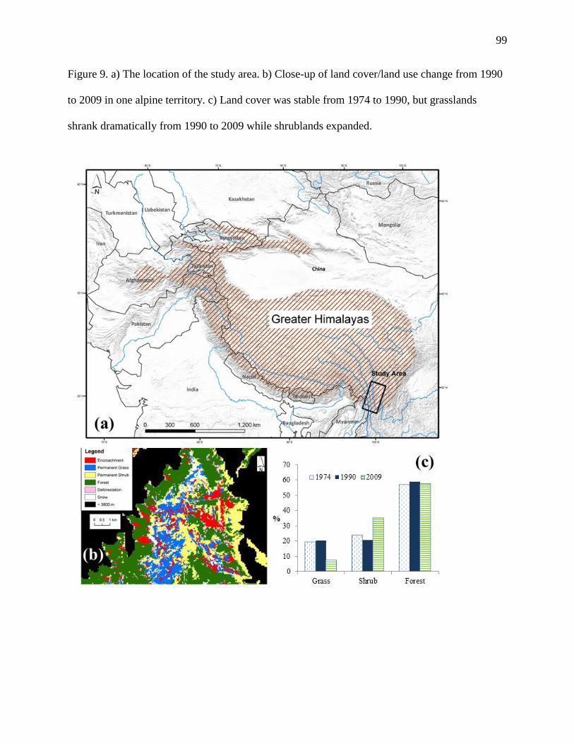
99
Figure 9. a) The location of the study area. b) Close-up of land cover/land use change from 1990
to 2009 in one alpine territory. c) Land cover was stable from 1974 to 1990, but grasslands
shrank dramatically from 1990 to 2009 while shrublands expanded.

100
Figure 10. a) Encroachment rates were highly variable throughout the study area, with the
northern and eastern regions suffering the highest encroachment rates. b) Shrub encroachment
rates were negatively correlated with the proportion of spring snow cover and positively
correlated with proportions of 1990 woody vegetation cover. Encroachment was related to c)
elevation and d) aspect, with meadows in lower elevations of the alpine zone (4000-4200 m) and
drier south facing slopes more subject to encroachment.

101
Figure 11. a) Higher grazing intensities close to the national highway increased shrub
encroachment rates; b) Relationships between encroachment and burning, and encroachment and
abandonment indicate that recent local-scale burning and pasture abandonment did not influence
regional patterns of shrub encroachment.

102
Figure 12. Average a) daily low and b) daily high temperatures (°C) at 3320 m and 4000m.Total
c) rainfall (mm) and d) snowfall (mm) measured at Deqin climate station. May average daily low
temperatures in the alpine zone from (e) early in the study period (1959-1968) and (f) late in the
study period (1999–2008).

103
Figure 13. Synthesis of land cover, land use, and climate change from 1951 to 2009.

104
Figure 14. Interactions between social, climate and alpine sub-systems during a) the feudal era,
b) the collectivization period and c) following decollectivization.

105
Chapter 3: Sacred forests are keystone structures for forest bird conservation
in southwest China’s Himalayan mountains
Abstract
Identifying and protecting “keystone structures” is essential to maintain biodiversity in an
increasingly human-dominated world. Sacred forests, i.e. natural areas protected by local people
for cultural or religious regions, may be keystone structures for forest birds in the Greater
Himalayas, but there is limited understanding of their use by bird communities at different
spatial scales. We surveyed birds and their habitat in and adjacent to six Tibetan sacred forests in
northwest Yunnan China, a biodiversity hotspot. Our goal was to understand the ecological and
conservation role of these remnant forest patches for forest birds. We found that sacred forests
supported a significantly different bird community than the surrounding matrix, and had higher
bird species richness at plot, patch, and landscape scales. Furthermore, while we encountered a
single matrix bird community outside the scared forests, the sacred forests themselves exhibited
high within- and between-patch heterogeneity, and supported at least two distinct sacred forest
bird communities. Finally, we found an increased use of the sacred forests and their edges during
2010, a severe drought year in Yunnan Province, indicating that sacred forests may serve as
refuges during extreme weather years. While bird community composition was primarily driven
by the vertical structure of the vegetation, plots with the largest diameter trees and the most
bamboo coverage had the highest bird diversity and abundance, indicating the importance of
protecting old-growth forest ecosystems for Himalayan forest birds. Old-growth forest clearing
and degradation have accelerated throughout the Himalayas, and our results offer hope for forest
birds, in that existing sacred forests do protect a variety of habitat niches and increase bird
diversity at multiple spatial scales. As population growth and rapid economic development

106
continues throughout the Himalayas, sacred areas can represent an important opportunity for
biological conservation at the local, landscape and regional scales.

107
Introduction
As humans consume an ever-increasing proportion of the Earth’s resources, biodiversity
declines at an accelerating rate (Chapin et al. 2000; Foley et al. 2005), making the protection of
“keystone structures”, i.e., discrete spatial features that maintain biodiversity at multiple spatial
scales, evermore important (Belsky & Canham 1994; Tews et al. 2004; Manning et al. 2006;
Stagoll et al. 2012). For example, forest gaps, large trees, and temporary wetlands are keystone
structures whose presence adds heterogeneity to the resources available in the landscape,
facilitating greater species richness. The question is how to identify such keystone structures, and
how to protect them.
Sacred forests, i.e., natural areas protected by local people for cultural or religious
reasons (Dudley et al. 2009), may be keystone structures for biodiversity in traditional
landscapes around the world. Sacred forests are numerous, dispersed across a broad range of
topographic and micro-climatic conditions, and range in size from a single hectare to thousands
of square kilometers (Ormsby 2011). As such, they likely serve multiple ecological functions,
including as corridors, refugia, and source habitats (Bhagwat & Rutte 2006). Sacred forests may
be critical components of protected area networks, but we have little understanding of their
potential role for biodiversity conservation, especially in the less-studied biodiversity hotspots.
The traditional land management systems that sustain sacred forests may create optimum
conditions for species diversity at multiple spatial scales. Sacred forests are typically managed by
communities (Dudley et al. 2009) and often experience a gradient of human disturbance
(UNESCO-MAB 2003), where a variety of organisms can respond to and thrive in variable
resource conditions (Belsky & Canham 1994). In addition, sacred forests are typically embedded
in landscapes with matrix habitats that are hospitable to at least some species, and thus
conventional assumptions of patch size and fragmentation effects (MacArthur & Wilson 1967)

108
may not apply (Prugh et al. 2008). Furthermore, the edges between sacred forests and their
matrix are often not abrupt barriers, but a gradient of disturbance to levels characteristic of the
surrounding matrix. These edges may serve as “ecotones”, facilitating ecological interactions
between the patch and the matrix, and offering supplementary resources not available in the core
habitats (Ries et al. 2004). However, despite their potential importance for species dispersal and
persistence, we have little understanding of how sacred forests are influenced by patch size, edge
effects, and interactions between patch and matrix habitats.
One region where sacred forests are relatively common are the Himalayan mountains
(Peng et al. 2003; UNESCO-MAB 2003; Xu et al. 2005; Salick et al. 2007; Mallarach 2008;
Barbhuiya et al. 2010). Several ethnic minority groups recognize sacred areas as part of their
religion, including sacred beyuls (which protect entire valleys), sacred mountains (10s to 100s of
km2), and village-level sacred forests (1 to 1000 ha). The Himalayan mountains also contain
three biodiversity hotspots (Myers et al. 2000) and forest birds are of special conservation
concern (Renner 2011). The region exhibits high levels of bird diversity and endemism (Acharya
et al. 2011; Renner & Rappole 2011), and rank highest in global assessments of threatened bird
species richness (Grenyer et al. 2006). Many forest bird species in the Greater Himalayas follow
a sino-Himalayan distribution (Renner 2011; Renner & Rappole 2011), which includes the
Himalayan range, the mountains of southwest China, and the Qinghai Tibetan plateau (Fig. 15a).
Forest degradation has accelerated throughout this region in recent decades (Spehn et al. 2010;
Brandt et al. 2012), destroying bird habitats (Dumbacher et al. 2011). Sacred areas may be
critical for bird conservation throughout this rapidly changing region, but their importance for
Himalayan forest bird communities across multiple spatial extents is not well understood.

109
Our overarching objective was to understand the role of sacred forests for the
conservation of Himalayan forest birds. We studied bird communities within and outside of
Tibetan sacred forests in northwest Yunnan, China, with the following specific objectives:
1. determine whether bird community composition and diversity is different within sacred
forests compared to the surrounding matrix,
2. identify the critical habitat characteristics structuring bird diversity, abundance, and
community composition, and
3. investigate how patch size and edge habitats influence bird community composition,
diversity and abundance patterns.
Study Area
Our study area is in Shangrila, northwest (NW) Yunnan Province, China (Fig. 15a). NW
Yunnan is a biodiversity hotspot in the southeastern sub-Himalayan mountains, bordering
Myanmar, Tibet and Sichuan Province. Three major rivers (the Yangtze, Mekong, and Salween)
create steep gorges, with elevations ranging from 1,800 to 6,740 m, creating a large array of
ecological niches in a relatively small area.
NW Yunnan has great importance for local, regional, and global bird diversity. First, it is
a center of bird endemism (Lei et al. 2003). Second, it is part of the East Asian migratory flyway,
providing important stop-over habitat for long-distance migrants (Cheng 1987). Third, it lies at
the confluence of the Palearctic, Himalayan, and Indo-malay zoogeographic regions, and thus
provides habitat for birds with distinct ecological and evolutionary histories (Renner 2011).
NW Yunnan’s avifauna is one the poorest understood on Earth (Renner & Rappole
2011), and it is likely that forest birds face serious threats. Large expanses of NW Yunnan’s
forests were clear-cut by state logging companies from the 1960s through the 1990s to fuel

110
China’s national development. Despite a ban on commercial logging in 1998 and heavy
investment in reforestation and protected areas (Liu et al. 2008), old-growth forests continue to
be logged and the ecological integrity of the new forests is unclear (Xu 2011; Brandt et al. 2012).
NW Yunnan is home to several ethnic minority groups that recognize sacred areas as part
of their religion (Xu et al. 2005). In particular, Tibetans have a complex sacred site system that
includes large Tibetan sacred mountains (tens to hundreds of square kilometers) and hundreds of
smaller community-based sacred forests (1 to 1,000 ha) at lower elevations (Peng et al. 2003;
Shen et al. 2012). Vegetation communities in Tibetan sacred forest sites have higher vegetation
species richness, diversity, and endemism than randomly selected non-sacred sites (Anderson et
al. 2005), and larger and denser trees (Salick et al. 2007). However, little is known about the
importance of Tibetan sacred forests for taxa other than plants.
Methods
Avifaunal sampling
We conducted breeding bird point count surveys at six sacred forest sites that ranged in
size from 13 to 75 ha (Fig. 15b). We surveyed a total of 62 plots, including 35 within the sacred
forests, 9 edge plots (60 m away from the sacred forest boundary), and 18 matrix plots (260 and
520 m from the boundary) (Fig. 15c). Plots were placed at least 200 m apart, along walking paths
when possible. At the plot center, we surveyed birds at least twice per year during the breeding
season (May 18-June 30) in 2010 and 2011. Surveys consisted of 50-m radius, 10-minute point
counts following standardized methods (Ralph et al. 1993), and included an estimate of distance
to bird using a hand-held laser rangefinder (Buckland et al. 2001). All point counts were
conducted by JSB and EMW.
Habitat structure

111
Vegetation composition and structure was measured at each point-count station according
to standardized protocols (Ralph et al. 1993; Martin et al. 1997) from June to August of 2010.
Within each point-count station, we measured four 5-m radius subplots (Ralph et al. 1993). The
initial sub-plot was located at the center of the point-count station, and the remaining three
subplots were located 30-m away at 0º, 120º and 240º. Slope, aspect and basal area (using a 10-
or 20-factor basal area per ft2 prism) were measured at the center point of each subplot. Canopy
coverage (using a densitometer) and foliage height diversity (in 0.3-m sub-sections) was
measured at the north, east, south, and west edge of each of the four subplots. Ocular estimates
for the sub-canopy layer (0.5-5 m) and the ground layer (0-0.5 m) were collected at each subplot.
Finally, we recorded all species of trees and shrubs, and the heights and dbh of the three tallest
and three largest-diameter trees, encountered in the entire 50-m radius plot.
Data Analysis
Differences between sacred forest and matrix habitats
We estimated differences in detection probabilities among habitats, and between years
based on our distance measurements and made density adjustments for those species for which
we had sufficient observations (>75) in each year (Buckland et al. 2001). We lumped edge plots
with matrix plots to estimate a species detection curve for sacred or non-sacred (i.e., edge and
matrix plots) habitats because matrix and edge habitat characteristics were similar in bird
detectability. There was a single species with sufficient observations in both 2010 and 2011
(Blyth’s Leaf Warbler (Phylloscopus reguloides)), and an additional species with sufficient
observations in 2010 only (Hume’s Leaf Warbler (Phylloscopus humei). Three models were used
to fit the detection function (Buckland et al. 2001) and the best model was selected using the
Akaike's Information Criterion (AIC) (Burnham & Anderson 2002).

112
We compared bird diversity and abundance among habitat types and between years at
three different spatial scales: plot, patch and landscape. At the plot scale, we compared raw
values of observed bird species richness, Shannon index, and absolute abundance in sacred,
matrix and edge habitats. Differences among habitat types were tested using a one-way analysis-
of-variance (ANOVA) and pairwise comparisons (Tukey multiple comparisons of means). At the
patch scale (n=6), we compared sacred and matrix/edge (lumped together for rarefaction)
habitats using observed species richness, rarefied species richness, and rarefied Shannon index,
all standardized by the number of individuals, derived from sample-based rarefaction curves
constructed in EstimateS v.7 (Colwell 2009). Differences at the patch scale were tested using
paired two-sample student’s t-tests. At the landscape scale, we calculated rarefied species
richness, rarefied Shannon index, and estimated total species richness (using the Jackknife 1
estimator) (Colwell 2009; González-Oreja et al. 2010). Patterns of bird diversity according to the
Shannon Index were consistently similar to raw and rarefied species richness, and therefore only
raw and rarefied species richness were reported here.
To determine whether bird species assemblages differed among habitats and sacred
forests, we removed rare species (less than 3 observations per year) from our multivariate dataset
and computed a Bray-Curtis similarity index on square root-transformed abundance data (Carr
1997). We then used non-metric multidimensional scaling (NMDS) to create a graphical
representation of the resemblance matrix (Kruskal 1964). Bird assemblage differences among a)
habitats and b) sacred forests were tested for using an analysis of similarity (ANOSIM). We used
a Bonferonni adjusted alpha value for pairwise comparisons among the three habitats (p = 0.05/3
= 0.016). NMDS and ANOSIM analyses were conducted using PRIMER v6 (Clarke & Gorley
2006).

113
Habitat selection
We used step-wise multiple linear regression to determine the most important
environmental variables influencing bird diversity and abundance at the plot scale. The best
model was selected using the Akaike's Information Criterion (AIC) (Burnham & Anderson
2002). To investigate the importance of patch size on species richness, we calculated Pearson’s
correlations between patch size and raw species richness. These analyses were performed in the
statistical package R version 2.8.1. To identify the most prominent habitat gradients and the most
important variables driving those gradients, we performed principal components analysis (PCA,
using PRIMER v6 (Clarke & Gorley 2006)) on the habitat variables that were both uncorrelated
and known to be important for bird communities according to the regression analysis. To
understand the relationship between the prominent habitat gradients and bird community
composition we performed canonical correspondence analysis (CCA in PC-ORD 6.04), which
constrains habitat gradients by the bird species data.
Results
Differences between sacred forest and matrix habitats
Habitat
We surveyed 62 plots that captured a wide range of variability in vegetation disturbance,
structure and species composition (Appendix 3). PCA identified two prominent habitat gradients
in our study area (Fig. 16a). The first axis (eigenvalue=3.59, explaining 44.8% of the variance)
corresponded to differences between sacred and matrix habitats, which had significantly different
vegetation composition and structure in the canopy, sub-canopy and ground layers (Appendix 4).
The first axis had high vertical structure (foliage height diversity), canopy cover and coarse
woody debris on at low values on Axis 1, and high proportions of bare soil and multiple-

114
stemmed woody vegetation in the ground layer (0 – 0.5 m) at high values on Axis 1. The second
axis of the PCA (eigenvalue=1.51, explaining 18.9% of the variance) represented a within-sacred
forest gradient, with dense understory vegetation (i.e., high proportions of sub-canopy coverage
and bamboo) corresponding to high values of Axis 2, while those with a more open understory
(high herbaceous cover and coarse woody debris in the ground layer) corresponding to low
values.
Birds
We observed a total of 81 species exhibiting breeding behavior (Appendix 5), ranging
from a few very common species (a total of 7 species detected > 100 times) to several rarely-
detected species (a total of 35 species observed 10 times or less). Detection probability was 5%
to 21% higher in the matrix than in the sacred forests. Detection probability was 10% to 17%
lower in 2010 than in 2011, and therefore we performed all analyses separately for the two years.
We used raw counts for the statistical analyses because sample size was too low to estimate
density for most species.
Species composition of the bird communities overlapped between the sacred, edge, and
matrix habitats (Fig. 16b), but still exhibited statistically significant patterns (NMDS, 2D
stress=0.21, ANOSIM Global R=0.254, p=0.001). Edge and matrix plots shared the same bird
community (p=0.51), while sacred forest bird communities were distinct from edge (R=0.227,
p=0.005) and matrix (R=0.37, p=0.001) communities. Furthermore, different sacred forests
supported distinct bird assemblages. Species composition was significantly different in five of 15
pairwise comparisons (ANOSIM, Global R=0.22, p=0.001), indicating that the sacred forests as a
whole provided habitat for more than one bird community.

115
We measured differences in bird species richness at three spatial scales. At the plot scale,
mean species richness was higher in sacred forests (mean (SD) = 13.3 (3.1)) than in edge (mean
= 11.1 (2.9), p = 0.084) and matrix (mean = 9.64 (1.9), p < 0.001) (Fig. 17a). Bird abundance
was slightly higher in sacred than in edge or matrix, but these differences were not significant (p
= 0.53 and 0.33, respectively).
Since edge and matrix were always similar in terms of bird species composition and
diversity, we aggregated edge and matrix plots into a single “matrix” class at the patch and
landscape scales, which allowed us to build rarefaction curves and thereby adjust for differences
in sampling effort and observed individuals. At the patch scale, sacred forest patches had higher
mean rarefied species richness (mean (SD) = 28 (6.8)) than the matrix (mean = 21 (5.8) (p <
0.001)) (Fig. 17b). At the landscape scale, bird species accumulated fastest in the sacred forest
habitat (Fig. 17c) and rarefied species richness (rarefied to 824 individuals) was higher in the
sacred (mean (SD) = 59 (4.1)) than the matrix (mean = 53(4.1)).
Habitat Selection
Four variables were selected among the candidate variables in the stepwise regression
(Appendix 4) as important predictors of species richness: the diameter of the largest tree, percent
bamboo, percent ground cover of coarse woody debris, and percent sapling cover (Stepwise
Regression AIC=112, Adj. R2=0.46, p<0.0001). In simple linear regression models to predict
bird abundance, only one variable, the diameter of the largest tree, was a significant predictor of
abundance (Adj. R2=0.20, p=0.00018).
The canonical correlation analysis indicated that habitat gradients and species
composition were highly correlated (Axis 1 Pearson’s r >0.95, Axis 2 Pearson’s r =0.718, Fig.
18). While several common generalist species (e.g., Hume’s and Blyth’s Leaf Warblers) were

116
detected in all habitats, many species were clearly associated with either sacred forests or matrix.
Axis 1 (Eigenvalue=0.480, explaining 14 % of the variance in the species data) captured a
gradient between birds associated with the matrix habitats at high values (e.g., White-bellied
Redstart (Hodgsonius phaenicuroides), White-tailed Rubythroat (Luscinia pectoralis), and
Common Stonechat (Saxicola torquata), and those associated with the sacred forests at low
values (e.g., Mrs Gould’s Sunbird (Aethopyga gouldiae), Blood Pheasant (Ithaginis cruentus),
Chinese Thrush (Turdus mupinensis), Grey-crested Tit (Pyrrhula erythaca), and Giant
Laughingthrush (Garrulax maximus). Foliage height diversity had the highest correlation with
Axis 1 (r = -0.525), indicating that it explained the highest variance in the species data. Axis 2
(Eigenvalue=0.114, explaining 3.3% of the variation in the species data) captured a gradient of
within-sacred forest habitats, and birds associated with dense understory cover (e.g., Giant
Laughingthrush, Lady Amherst’s Pheasant (Chrysolophus amherstiae), and Yellowish-bellied
Bush Warbler (Cettia acanthizoides) had high values of Axis 2, while birds associated with large
trees, high canopy cover and coarse woody debris (e.g., Yunnan Nuthatch (Sitta yunnanensis),
Great Spotted Woodpecker (Dendrocopos major), and several tit species) had low values.
Edge effects and patch-matrix interactions
To investigate whether edges influenced bird diversity patterns, we regressed bird
richness and abundance against distance from the edge of a sacred forest. Within sacred forest
patches, species richness increased with a plot’s distance to the edge of the sacred forest patch
(R2=0.11, p=0.06). For the matrix, we found the opposite relationship. Matrix bird diversity was
highest at the edge, but decreased with distance from the sacred forest (R2=0.17, p=0.03). There
was no relationship between bird abundance and distance from the edge.

117
The correlation between patch size and bird species richness was positive and significant
for patch size and raw species richness in the sacred forest patches (r=0.79, p=0.03) and in the
matrix plots associated with each sacred forest patch (r=0.80, p=0.05). However, when
standardizing for sample effort and number of individuals, the correlations between patch size
and rarefied species richness were not significant.
Differences between 2010 versus 2011
We encountered significantly more birds in 2010 than in 2011 (p < 0.001) in all three
habitats (sacred, matrix, and edge). There were a total of 15 species (including Greenish Warbler
(Phylloscopus trochiloides), Bar-tailed Treecreeper (Certhia himalayana) and Grey-chinned
Minivet (Pericrocotus solaris)) that were observed in 2010 but not 2011, and another 9 species
(including Lady Amherst’s Pheasant, Chinese Thrush, Giant Laughingthrush, and Chestnut-
vented Nuthatch (Sitta nagaensis)) that were observed in both years, but were considerably (>
3x) more abundant in 2010 than 2011. Plot-scale bird richness was significantly higher in 2010
than in 2011 in sacred and edge, but not in matrix (Fig. 19a). Estimated total species richness
curves indicated that species accumulated at the same rate in both years in both the matrix and
sacred habitats, but species accumulated at a much faster rate in edge habitats in 2010 versus
2011 (Fig. 19b).
Discussion
Sacred Forests as Keystone Structures
Our results indicated that Tibetan sacred forests conserved old-growth forest
characteristics and protected unique forest bird communities in the Chinese Himalayan
mountains. In addition, sacred forests had the highest bird diversity of all habitats at multiple
spatial scales and in both years. Since detection probabilities were considerably lower in the

118
sacred forests compared to their matrix, it is likely that our estimates of differences are
conservative, and that sacred forests are even more important than indicated by the raw data.
Sacred forests exhibited several characteristics of keystone structures (Tews et al. 2004).
First, sacred forests maintained higher bird and vegetation diversity despite being small in
proportion to the adjacent matrix habitats that make up the majority of the Shangrila landscape.
Second, the bird diversity was not dependent on a particular tree species or forest community,
but instead associated with structural characteristics that increased habitat heterogeneity. Finally,
the positive relationship between habitat heterogeneity and bird diversity was consistent across
multiple spatial scales.
Keystone structures maintain biodiversity because of both within-patch and between-
patch heterogeneity. The Tibetan sacred forests that we studied have been protected from clear-
cut logging, but do experience a range of human disturbance, including occasional selective
logging, NTFP collection, and grazing. Thus, they are structurally complex and composed of a
mixture of successional and old-growth forests. This within-patch heterogeneity is important to
create an environment where a variety of organisms can respond to ˗ and thrive in - the variable
resource conditions of the patch (Belsky & Canham 1994).
In terms of between-forest heterogeneity, although the sacred forests were relatively close
to each other (<20 km) and at similar elevation (3200 to 3800 m), they contained a variety of
habitat niches due to micro-topographic and micro-climatic variability. In contrast, the
surrounding matrix, which has been subject to a range of high-intensity subsistence land-use
pressures including logging, non-timber forest resource collection, and grazing, exhibited a
relatively homogeneous matrix habitat. As a result, while the matrix habitats had a single,

119
homogeneous bird community, sacred forests supported a wider range of bird species, and two
distinct sacred forest bird communities.
Habitat Selection of Old-growth Forest Characteristics
Our results indicated the importance of mature forest ecosystems over secondary or
disturbed forest habitats. The relatively large range in vertical complexity (i.e., foliage height
diversity, MacArthur & MacArthur 1961) of our survey plots was the main characteristic
structuring bird species composition, while old-growth trees, bamboo groves and coarse woody
debris were the most important factors determining high species richness and abundance. In
some ecosystems, bird diversity peaks in secondary growth stages (Keller et al. 2003; Schieck &
Song 2006), while in other ecosystems, primary forests support unique, high-diversity bird
communities (Barlow et al. 2007; Ding et al. 2008). Old-growth forests, including large trees and
bamboo groves (a native understory component), have been heavily exploited for both
subsistence and commercial use in this region (Xu 2011; Brandt et al. 2012), Our results suggest
that the protection of forests that retain old-growth characteristics should be a high priority for
forest bird conservation in this biodiversity hotspot.
Bird diversity at the plot scale was also positively associated with high proportions of
sapling cover. Post-logging tree regeneration in the matrix is limited due to logging practices that
leave no mature trees as sources for natural regeneration, and due to grazing which destroys any
seedlings and saplings which do grow, allowing shrub and scrub-forest communities to persist
for decades following forest clearing (Xu 2011). Land management practices that encourage tree
regeneration in the matrix would benefit forest bird communities.
Influence of edge habitats and patch size on bird community patterns

120
In some ecosystems, edges serve as an ecotone, providing supplementary resources that
are not present in the core or matrix habitats, resulting in relatively high species richness and
abundance and distinct species assemblages along edges (Ries et al. 2004). Surprisingly, our
results suggested that sacred forest edges were not a distinct habitat, but rather an intermediate
and overlapping zone between sacred and matrix habitats. In addition, species richness increased
moving deeper into the core of the sacred forests, indicating that interior forests contained higher
quality habitat than edges.
Thus, large remnant old-growth forest patches are especially important for birds in our
study area. Generally speaking, the larger the patch the higher the ratio of core forest to edge
habitats (Turner et al. 2001). Furthermore, while even the smallest sacred forest patch that we
surveyed (13 h) had a bird community that was distinct from - and more diverse than - the
surrounding matrix, large patches supported more bird species, likely because they contained
more habitat niches (MacArthur & Wilson 1967) and supported more individual birds (More
Individuals Hypothesis (Srivastava & Lawton 1998)).
Differences between 2010 versus 2011
We found clear inter-annual differences in bird presence, abundance, and richness. Bird
abundance was higher in all habitats in 2010. In sacred and edge plots we also encountered
higher bird diversity in 2010, and the edge habitat had a higher rate of species accumulation.
Yunnan province as a whole experienced a severe drought in 2010, receiving 60% less rainfall
than normal during the 6 months leading up to the 2010 breeding season (Qiu 2010). However,
Shangrila weather station data indicated that the drought was less severe in our study area. The
typical effect of a drought is to reduce bird abundance and diversity in some habitats while other

121
habitats act as refugia (Albright et al. 2010). Our results indicated that sacred forests, and
especially their edges, may serve as refuges during extreme weather years.
Management Implications
Although in the past, sacred forests have proven to be remarkably resilient to social
change (Dudley et al. 2009), the current trend is towards cultural assimilation and the
degradation of sacred forests (Rutte 2011), and efforts to understand the underlying cultural
values and management mechanisms may be necessary if sacred forests are to persist. For
example, incorporating sacred forests into official protected area networks may not be desirable
from the community perspective, as it leads to a loss in legal ownership and property rights
(Bhagwat & Rutte 2006). Furthermore, as ecotourism expands, many communities exploit sacred
forests for commercial use as touristic destinations, which can lead to a fundamental change in
their meaning, management and ecological function (Barbhuiya et al. 2010)
Sacred forests are apparently keystone structures for forest birds in NW Yunnan, and,
potentially, throughout the Himalayas. Faced with rapid land use and climate change, it is
important to establish reserve networks that cover the entire range of elevations and aspects (Wu
et al. 2010), but establishing large, contiguous protected areas is challenging in this densely
inhabited landscape. Although China’s protected area system has expanded greatly since the
1980s, its effectiveness is limited (Tang et al. 2006). Sacred forests throughout the Greater
Himalayan region provide an existing network of native vegetation patches that protect a variety
of habitat niches, maintain biodiversity at multiple spatial scales, and may even function as
refugia during extreme weather years.
References

122
Acharya, B. K., N. J. Sanders, L. Vijayan, and B. Chettri. 2011. Elevational Gradients in Bird
Diversity in the Eastern Himalaya: An Evaluation of Distribution Patterns and Their
Underlying Mechanisms. Plos One 6.
Albright, T. P., A. M. Pidgeon, C. D. Rittenhouse, M. K. Clayton, C. H. Flather, P. D. Culbert,
B. D. Wardlow, and V. C. Radeloff. 2010. Effects of drought on avian community
structure. Global Change Biology 16:2158-2170.
Anderson, D., J. Salick, R. K. Moseley, and O. Xiaokun. 2005. Conserving the sacred medicine
mountains: a vegetation analysis of Tibetan sacred sites in Northwest Yunnan.
Biodiversity and Conservation 14:3065-3091.
Barbhuiya, A., M. Khan, A. Arunachalam, S. Prabhu, and V. Chavan. 2010. Sacred Groves:
Informal Protected Areas in the High Altitudes of Eastern Himalaya, Arunachal Pradesh,
Northeast India: Traditional Beliefs, Biodiversity and Conservation. Pages 131-146 in A.
O'Reilly, and D. Murphy, editors. National Parks: Biodiversity, Conservation and
Tourism.
Barlow, J., L. A. M. Mestre, T. A. Gardner, and C. A. Peres. 2007. The value of primary,
secondary and plantation forests for Amazonian birds. Biological Conservation 136:212-
231.
Belsky, A., and C. Canham. 1994. Forest Gaps and Isolated Savanna Trees: An application of
patch dynamics in two ecosystems. BioScience 44:77-84.
Bhagwat, S., and C. Rutte. 2006. Sacred groves: potential for biodiversity management. Frontiers
in Ecology and the Environment 4:519-524.

123
Brandt, J. S., T. Kuemmerle, H. Li, G. Ren, J. Zhu, and V. C. Radeloff. 2012. Using Landsat
imagery to map forest change in southwest China in response to the national logging ban
and ecotourism development. Remote Sensing of Environment 121:358-369.
Buckland, S., D. Andersong, K. Burnham, and J. Laake 2001. Distance Sampling. Estimating
Abundance of Biological Populations, London.
Burnham, K., and D. Anderson 2002. Model selection and multimodal inference: a practical
information theoretic approach. Springer-Verlag, USA.
Carr, M. 1997. PRIMER user manual (Plymouth routines in multivariate ecological research). .
Plymouth Marine Laboratory, Plymouth, UK.
Chapin, F., E. Zavaleta, V. Eviner, R. Naylor, P. Vitousek, H. Reynolds, D. Hooper, S. Lavorel,
O. Sala, S. Hobbie, M. Mack, and S. Diaz. 2000. Consequences of changing biodiversity.
Nature 405:234-242.
Cheng, T.-h. 1987. A synopsis of the Avifauna of China. Parey, Beijing.
Clarke, K., and R. Gorley. 2006. PRIMER v6: User Manual/Tutorial. PRIMER-E, Plymouth.
Colwell, R. 2009. EstimateS: Statistical estimation of species richness and shared species from
samples. Version 8.2. User's Guide.
Ding, T., H. Liao, and H. Yuan. 2008. Breeding bird community composition in different
successional vegetation in the montane coniferous forests zone of Taiwan. Forest
Ecology and Management 255:2038-2048.
Dudley, N., L. Higgins-Zogib, and S. Mansourian. 2009. The Links between Protected Areas,
Faiths, and Sacred Natural Sites. Conservation Biology 23:568-577.

124
Dumbacher, J., J. R. Miller, M. Flannery, and X. Yang. 2011. Avifauna of the Gaoligong Shan
Mountains of Western China: A Hotspot of Avian Species Diversity. Ornithological
Monographs 70:30-63.
Foley, J. A., R. DeFries, G. P. Asner, C. Barford, G. Bonan, S. R. Carpenter, F. S. Chapin, M. T.
Coe, G. C. Daily, H. K. Gibbs, J. H. Helkowski, T. Holloway, E. A. Howard, C. J.
Kucharik, C. Monfreda, J. A. Patz, I. C. Prentice, N. Ramankutty, and P. K. Snyder.
2005. Global consequences of land use. Science 309:570-574.
González-Oreja, J., C. Garbisu, S. Mendarte, A. Ibarra, and I. Albizu. 2010. Assessing the
performance of nonparametric estimators of species richness in meadows. Biodiversity
and Conservation 19:1417-1436.
Grenyer, R., C. D. L. Orme, S. F. Jackson, G. H. Thomas, R. G. Davies, T. J. Davies, K. E.
Jones, V. A. Olson, R. S. Ridgely, P. C. Rasmussen, T.-S. Ding, P. M. Bennett, T. M.
Blackburn, K. J. Gaston, J. L. Gittleman, and I. P. F. Owens. 2006. Global distribution
and conservation of rare and threatened vertebrates. Nature 444:93-96.
Keller, J., M. Richmond, and C. Smith. 2003. An explanation of patterns of breeding bird species
richness and density following clearcutting in northeastern USA forests. Forest Ecology
and Management 174:541-564.
Lei, F.-M., Y.-H. Qu, Q. Tang, and S. An. 2003. Priorities for the conservation of avian
biodiversity in China based on the distribution patterns of endemic bird genera.
Biodiversity and Conservation 12:2487-2501.
Liu, J. G., S. X. Li, Z. Y. Ouyang, C. Tam, and X. D. Chen. 2008. Ecological and socioeconomic
effects of China's policies for ecosystem services. Proceedings of the National Academy
of Sciences of the United States of America 105:9477-9482.

125
MacArthur, R., and E. Wilson 1967. The theory of island biogeography. Princeton University
Press, Princeton, NJ.
Mallarach, J., editor. 2008. Protected Landscapes and Cultural and Spiritual Values. World
Conservation Union.
Manning, A. D., J. Fischer, and D. B. Lindenmayer. 2006. Scattered trees are keystone structures
– Implications for conservation. Biological Conservation 132:311-321.
Martin, T., C. Paine, C. Conway, W. Hochachka, P. Allen, and W. Jenkens. 1997. BBird Field
Protocol. Montana Coop. Wildlife Research Unit, Missoula, Montana.
Myers, N., R. Mittermeier, C. Mittermeier, G. A. B. da Fonseca, and J. Kent. 2000. Biodiversity
hotspots for conservation priorities. Nature 403:853-858.
Ormsby, A. 2011. The impacts of global and national policy on the management and
conservation of sacred groves of India. Human Ecology:783-793.
Peng, L., W. Ning, Y. Zhaoli, and P. Shengji. 2003. Sacred Sites in Northwest Yunnan, China in
C. Lee, and T. Schaaf, editors. International Workshop on the Importance of Sacred
Natural Sites for Biodiversity Conservation. UNESCO, Kunming.
Prugh, L., K. Hodges, A. Sinclair, and J. Brashares. 2008. Effect of habitat area and isolation on
fragmented animal populations. PNAS 105:20770-20775.
Qiu, J. 2010. China drought highlights future climate threats. Nature 465:142-143.
Ralph, C., G. Guepel, P. Pyle, T. Martin, and D. DeSante. 1993. Handbook of field methods for
monitoring landbirds. Gen. Tech. Rep. PSW-GTR-144.
Renner, S. C. 2011. Bird Species-Richness Pattern in the Greater Himalayan Mountains—A
General Introduction. Ornithological Monographs 70:1-9.

126
Renner, S. C., and J. H. Rappole. 2011. Bird Diversity, Biogeographic Patterns, and Endemism
of the Eastern Himalayas and Southeastern Sub-Himalayan Mountains. Ornithological
Monographs 70:153-166.
Ries, L., R. J. Fletcher, J. Battin, and T. D. Sisk. 2004. Ecological responses to habitat edges:
Mechanisms, models, and variability explained. Annual Review of Ecology Evolution
and Systematics 35:491-522.
Rutte, C. 2011. The sacred commons: Conflicts and solutions of resource management in sacred
natural sites. Biological Conservation 144:2387-2394.
Salick, J., A. Amend, D. Anderson, K. Hoffmeister, B. Gunn, and F. Zhendong. 2007. Tibetan
sacred sites conserve old growth trees and cover in the easter Himalayas. Biodiversity
and Conservation 16:693-706.
Schieck, J., and S. Song. 2006. Changes in bird communities throughout succession following
fires and harvest in boreal forests of western North America: literature review and meta-
analyses. Can. J. For. Res. 36:1299-1318.
Shen, X., Z. Lu, S. Li, and N. Chen. 2012. Tibetan Sacred Sites: Understanding the Traditional
Management System and its Role in Modern Conservation. Ecology and Society 17.
Spehn, E., K. Rudmann-Maurer, C. Korner, and D. Maselli, editors. 2010. Mountain Biodiversity
and Global Change, Basel.
Srivastava, D. S., and J. H. Lawton. 1998. Why more productive sites have more species: An
experimental test of theory using tree-hole communities. American Naturalist 152:510-
529.
Stagoll, K., D. B. Lindenmayer, E. Knight, J. Fischer, and A. D. Manning. 2012. Large trees are
keystone structures in urban parks. Conservation Letters:no-no.

127
Tang, Z., Z. Wang, C. Zheng, and J. Fang. 2006. Biodiversity in China's mountains. Frontiers in
Ecology and the Environment 4:347-352.
Tews, J., U. Brose, V. Grimm, K. Tielborger, M. Wichmann, M. Schwager, and F. Jeltsch. 2004.
Animal species diversity driven by habitat heterogeneity/diversity: the importance of
keystone structures. Journal of Biogeography 31:79-92.
Turner, M., R. Gardner, and R. O'Neill 2001. Landscape ecology in theory and practice: pattern
and process. Springer.
UNESCO-MAB. 2003. The Importance of Sacred Natural Sites for Biodiversity Conservation in
C. Lee, and T. Schaaf, editors. International Workshop on the Importance of Sacred
Natural Sites for Biodiversity Conservation. UNESCO, Kunming, China.
Wu, F., X. Yang, and J. Yang. 2010. Additive diversity partitioning as a guide to regional
montane reserve design in Asi: an example from Yunnan Province, China. Diversity and
Distributions 16:1022-1033.
Xu, J. 2011. China's new forests aren't as green as they seem. Nature Australia 477.
Xu, J., T. M. Ma, D. Tashi, Y. Fu, Z. Lu, and D. Melick. 2005. Integrating sacred knowledge for
conservation: cultures and landscapes in southwest China. Ecology and Society 10.

128
Figure 15. a) Location of Shangrila within the Greater Himalayan region, b) the six sacred forest
patches that were surveyed, and c) sampling plots within and outside of sacred forests. Matrix
plots were placed on transects at approximately 60, 260, and 510 m away from the edge of the
sacred forest.

129
Figure 16. Multivariate analyses of a) habitat gradients (PCA) and b) bird community
composition (NMDS).

130
Figure 17. Box plots of a) plot-scale bird species richness, b) patch-scale rarefied bird richness,
and c) rarefied species richness accumulation curves at the landscape scale (dotted lines are 95%
confidence intervals).

131
Figure 18. Canonical Correspondence Analysis demonstrates that Foliage Height Diversity was
the main characteristic structuring bird communities along Axis 1, while Axis 2 showed the
separation between two distinct sacred forest bird communities. Bird species indicated with 4-
letter species code. Full species names can be found in Appendix 5.

132
Figure 19. Inter-annual variability in a) plot-scale species richness and b) estimated total species
richness at the landscape scale.

133
Appendix 3. Description of the 62 plots sampled during the study.
Site
Class Plot General Habitat Type
Dominant Tree
Species
Foliage
Height
Diversity
Tree
Species
Richness
Shrub
Species
Richness
A Sacred AA1 Mid-successional forest Pinus densata 2.8 4 10
A Sacred AA2 Primary forest
Quercus
aquifolioides 3.0 7 12
A Sacred AA3 Scrub and saplings Pinus densata 2.7 6 12
A Sacred AA4 Primary forest
Quercus
aquifolioides 2.7 7 9
A Matrix AT1-260 Scrub forest na 1.1 4 7
A Matrix AT1-510 Scrub forest na 1.1 2 10
A Edge AT1-60 Scrub and saplings na 1.5 5 11
B Sacred BA1 Mid-successional mixed Betula platyphylla 2.7 8 11
B Sacred BA2 Primary forest
Picea likiangensis
var. linzhiensis 2.5 6 13
B Sacred BA3 Primary forest
Picea likiangensis
var. linzhiensis 2.6 6 16
B Sacred BA4 Primary forest
Picea likiangensis
var. linzhiensis 2.4 2 17
B Sacred BA5 Primary forest Sorbus multijuga 2.3 3 9
B Sacred BA6 Primary forest
Picea likiangensis
var. linzhiensis 3.5 4 10
B Sacred BA7 Primary forest
Picea likiangensis
var. linzhiensis 3.1 6 12
B Sacred BA8 Mid-successional mixed Tilia chinensis 2.4 5 15
B Sacred BA9 Mid-successional birch Betula platyphylla 2.8 6 14
B Matrix BAT1-260 Scrub forest na 1.0 2 14
B Matrix BAT1-510 Scrub forest na 1.3 3 17
B Matrix BAT2-260 Scrub forest na 0.7 2 9
B Matrix BAT2-510 Scrub forest na 0.4 4 14
B Edge BAT1-60 Scrub and saplings
Larix potaninii
var.macrocarpa 1.3 5 13
B Edge BAT2-60 Scrub and saplings na 1.7 3 12
H Sacred HA1 Early successional birch Betula platyphylla 2.4 6 12
H Sacred HA2 Mid-successional mixed
Picea likiangensis
var. linzhiensis 2.3 9 15
H Sacred HA3 Primary forest
Picea likiangensis
var. linzhiensis 2.7 7 13
H Sacred HA4 Primary forest
Picea likiangensis
var. linzhiensis 3.1 7 12
H Matrix HAT1-260 Scrub forest na 1.5 5 11
H Matrix HAT1-510 Scrub forest na 1.0 2 8
H Edge HAT1-60 Scrub and saplings na 1.4 6 17
J Sacred JA1 Mid-successional mixed
Larix potaninii
var.macrocarpa 1.4 3 10

134
J Sacred JA2 Early successional birch Betula platyphylla 2.8 7 14
J Sacred JA3 Early successional birch Betula platyphylla 2.7 5 12
J Matrix JAT1-260 Scrub forest na 0.0 2 8
J Matrix JAT1-510 Scrub forest na 0.5 3 15
J Edge JAT1-60 Scrub and meadow na 0.5 3 12
W Sacred WF1 Mid-successional birch Betula platyphylla 2.4 3 14
W Sacred WF2 Primary forest
Larix potaninii
var.macrocarpa 2.7 4 17
W Sacred WF3 Primary forest Quercus pannosa 2.8 4 10
W Sacred WF4 Primary forest Quercus pannosa 2.8 5 12
W Sacred WF5 Primary forest Quercus pannosa 3.1 4 13
W Sacred WF6 Primary forest Quercus pannosa 2.8 3 14
W Sacred WF7 Primary forest
Larix potaninii
var.macrocarpa 1.8 4 16
W Sacred WF8 Primary forest Quercus pannosa 2.5 4 14
W Matrix WAT1-260 Scrub and saplings Pinus densata 1.2 6 10
W Matrix WAT1-510 Scrub forest na 1.0 3 7
W Matrix WAT2-260 Scrub forest na 0.8 4 8
W Matrix WAT2-510 Scrub forest na 0.9 4 9
W Edge WAT1-60 Scrub and saplings
Larix potaninii
var.macrocarpa 1.5 4 8
W Edge WAT2-60 Scrub and saplings
Larix potaninii
var.macrocarpa 2.2 2 15
X Sacred XA1 Primary forest
Picea likiangensis
var. linzhiensis 2.4 6 18
X Sacred XA2 Primary forest Populus davidiana 2.2 6 11
X Sacred XA3 Primary forest
Picea likiangensis
var. linzhiensis 2.0 6 11
X Sacred XA4 Primary forest Salix delavayana 3.9 5 16
X Sacred XA5 Primary forest Acer caesium 2.5 7 12
X Sacred XA6 Primary forest Acer pectinatum 2.9 6 9
X Sacred XA7 Primary forest Salix delavayana 2.5 6 8
X Matrix XAT1-260 Mid-successional mixed Betula platyphylla 2.5 6 18
X Matrix XAT1-510 Mid-successional pine Pinus densata 2.3 6 18
X Matrix XAT2-260 Early successional mixed Pinus densata 2.2 3 11
X Matrix XAT2-510 Early successional pine Pinus densata 2.4 3 9
X Edge XAT1-60 Mid-successional pine Pinus densata 2.3 4 7
X Edge XAT2-60 Early successional pine Pinus densata 2.7 5 10

135
Appendix 4. The set of candidate variables chosen for the stepwise regression, with the
corresponding Adjusted R2 and significance values in the simple linear regressions to predict
plot-scale species richness; and means, standard deviations and significance values for each
variable in sacred versus matrix habitats.
Simple Linear
Regression
Analysis Sacred Matrix
Difference
between
Sacred and
Matrix
Variable Adj. R2 p Mean SD Mean SD p
Canopy Layer (> 5 m)
Biggest Tree (dbh) 0.31 < 0.01 63.4 39.7 23.7 24.1 < 0.01
Tallest Tree (m) 0.30 < 0.00 26.7 9.7 11.7 10.4 < 0.01
Foliage Height Diversity 0.13 < 0.01 3.1 0.7 1.8 0.4 < 0.01
Tree Species Richness 0.09 0.01 5.3 1.6 3.7 1.4 < 0.01
Canopy Cover (%) 0.04 0.06 54.9 27.6 12.8 21.7 < 0.01
Basal area (sq. ft./acre) 0.04 0.06 70.1 49.0 15.2 28.6 < 0.01
Sub Canopy Layer (0.5 - 5 m)
Bamboo Cover (%) 0.20 < 0.01 8.7 12.6 1.9 3.2 0.01
Subcanopy Cover (%) 0.07 0.02 62.4 10.5 52.0 15.2 < 0.01
Sapling Cover (%) 0.05 0.04 20.8 8.5 17.1 12.9 0.181
Ground Layer (0 - 0.5 m)
Downed Log Cover (%) 0.12 < 0.01 1.6 1.3 0.4 1.0 < 0.01
Bare ground (%) 0.12 < 0.01 0.3 0.6 6.5 7.9 < 0.01
Live Woody Plant Cover (%) 0.05 0.05 39.7 12.0 59.6 13.4 < 0.01

136
Appendix 5. Breeding birds observed during the study.
Total observations Total Total Proportional Total Total Proportional
Code Common name Latin name 2010 + 2011 Sacred Matrix+Edge Difference 1
2010 2011 Change 2
BTTC Bar-tailed Treecreeper Certhia himalayana 8 8 0 NO M/E 8 0 NO 2011
BWWB Bar-winged Wren-babbler Spelaeornis troglodytoides 3 2 1 2.0 3 0 NO 2011
BLDR Black Drongo Dicrurus macrocercus 1 1 0 NO M/E 0 1 NO 2010
BBTI Black-browed Tit Aegithalos bonvaloti 44 36 8 4.5 27 17 1.6
BLPH Blood Pheasant Ithaginis cruentus 21 19 2 9.5 12 9 1.3
BFRS Blue-fronted Redstart Phoenicurus frontalis 4 2 2 1.0 4 0 NO 2011
BLYW Blyth’s Leaf Warbler Phylloscopus reguloides 409 226 183 1.2 234 175 1.3
BRPB Brown Parrotbill Paradoxornis unicolor 5 3 2 1.5 3 2 1.5
BUBW Buff-barred Warbler Phylloscopus pulcher 79 64 15 4.3 54 25 2.2
CNTH Chestnut Thrush Turdus rubrocanus 24 23 1 23.0 19 5 3.8
CHTE Chestnut-headed Tesia Tesia castaneocoronata 18 9 9 1.0 10 8 1.3
CVNH Chestnut-vented Nuthatch Sitta nagaensis 16 14 2 7.0 12 4 3.0
CBAB Chinese Babax Babax lanceolatus 6 2 4 0.5 3 3 1.0
CHTH Chinese Thrush Turdus mupinensis 40 37 3 12.3 33 7 4.7
COTI Coal Tit Parus ater 54 35 19 1.8 28 26 1.1
COGR Collared Grosbeak Mycerobas affinis 9 9 0 NO M/E 6 3 2.0
EUCU Common Cuckoo Cuculus canorus 23 8 15 0.5 6 17 0.4
COPH Common Pheasant Phasianus colchicus 10 4 6 0.7 7 3 2.3
CORF Common Rosefinch Carpodacus erythrinus 238 73 165 0.4 166 72 2.3
COSC Common Stonechat Saxicola torquata 17 0 17 0.0 12 5 2.4
CBWP Crimson-breasted Woodpecker Dendrocopos cathpharius 1 1 0 NO M/E 0 1 NO 2010
DBRF Dark-browed Rosefinch Carpodacus nipalensis 2 2 0 NO M/E 2 0 NO 2011
DARS Daurian Redstart Phoenicurus auroreus 22 20 2 10.0 14 8 1.8
ELLT Elliot’s Laughingthrush Garrulax elliotii 174 67 107 0.6 136 38 3.6
EUJA Eurasian Jay Garrulus glandarius 4 4 0 NO M/E 2 2 1.0
EUTC Eurasian Treecreeper Certhia familiaris 7 6 1 6.0 0 7 0.0
FIRE Firethroat Luscinia pectardens 3 3 0 NO M/E 1 2 0.5
GILT Giant Laughingthrush Garrulax maximus 34 32 2 16.0 26 8 3.3
GOBU Godlewski’s Bunting Emberiza godlewskii 3 0 3 NO S 2 1 2.0
GSPW Golden Spectacled Warbler Seicercus burkii 205 152 53 2.9 132 73 1.8
GRPB Great Parrotbill Conostoma oemodium 1 1 0 NO M/E 1 0 NO 2011

137
1 Proportional Difference represents the total number of observations in sacred forests
divided by the total number of observations in matrix and edge habitats. NO M/E = Not
Observed in Matrix/Edge, NO S = Not Observed in Sacred.
2 Proportional Change represents the total observations in 2010 divided by the total
observations in 2011, to highlight interannual variability of different species. NO 2010 = Not
Observed in 2010, NO 2011 = Not Observed in 2011.
GSWP Great Spotted Woodpecker Dendrocopos major 13 11 2 5.5 7 6 1.2
GRTI Great Tit Parus major 18 12 6 2.0 15 3 5.0
GBTI Green-backed Tit Parus monticolus 8 3 5 0.6 4 4 1.0
GRNW Greenish Warbler Phylloscopus trochiloides 15 10 5 2.0 15 0 NO 2011
GBSH Grey-backed Shrike Lanius tephronotus 30 2 28 0.1 20 10 2.0
GCMV Grey-chinned Minivet Pericrocotus solaris 14 12 2 6.0 14 0 NO 2011
GCTI Grey-crested Tit Pyrrhula erythaca 56 56 0 NO M/E 34 22 1.5
GHBF Grey-headed Bullfinch Pyrrhula erythaca 62 57 5 11.4 37 25 1.5
GHPB Grey-headed Parrotbill Paradoxornis gularis 7 3 4 0.8 3 4 0.8
GHWP Grey-headed Woodpecker Picus canus 3 3 0 NO M/E 2 1 2.0
HUMW Hume’s Leaf Warbler Phylloscopus humei 280 151 129 1.2 196 84 2.3
INBR Indian Blue Robin Luscinia brunnea 30 27 3 9.0 19 11 1.7
LAPH Lady Amherst’s Pheasant Chrysolophus amherstiae 6 6 0 NO M/E 5 1 5.0
LBCR
Large-billed Crow
(tibetosinensis)
Corvus macrorhynchos
tibetosinensis 21 20 1 20.0 18 3 6.0
LBLW Large-billed Leaf Warbler Phylloscopus magnirostris 24 20 4 5.0 17 7 2.4
LRUW Lemon-rumped Warbler Phylloscopus proregulus 113 99 14 7.1 63 50 1.3
LECU Lesser Cuckoo Cuculus poliocephalus 4 0 4 NO S 0 4 NO 2010
LTMV Long-tailed Minivet Pericrocotus ethologus 40 34 6 5.7 24 16 1.5
GSUN Mrs Gould's Sunbird Aethopyga gouldiae 60 53 7 7.6 37 23 1.6
NOGO Northern Goshawk Accipiter gentilis 1 1 0 NO M/E 0 1 NO 2010
OBPI Olive Backed Pipit Anthus hodgsoni 15 0 15 0.0 9 6 1.5
OTDO Oriental Turtle Dove Streptopelia orientalis 57 42 15 2.8 34 23 1.5
PALW Palla's Leaf Warbler Phylloscopus proregulus 1 1 0 NO M/E 1 0 NO 2011
RECR Red Crossbill Loxia curvirostra 2 0 2 NO S 2 0 NO 2011
RTFC Red-throated Flycatcher Ficedula Parva 2 2 0 NO M/E 0 2 NO 2010
RBAC Rufous-breasted Accentor Prunella strophiata 6 0 6 0.0 3 3 1.0
RGFC Rufous-gorgeted Flycatcher Ficedula strophiata 1 1 0 NO M/E 1 0 NO 2011
RVTI Rufous-vented Tit Periparus rubidiventris 40 33 7 4.7 28 12 2.3
RVYU Rufous-vented Yuhina Yuhina occipitalis 13 9 4 2.3 4 9 0.4
RCFU Rusty-capped Fulvetta Schoeniparus dubia 10 10 0 NO M/E 0 10 NO 2010
SBMV Short-billed Minivet Pericrocotus brevirostris 2 2 0 NO M/E 0 2 NO 2010
SBFC Slaty Blue Flycatcher Ficedula tricolor 57 51 6 8.5 37 20 1.9
SLFC Slaty-backed Flycatcher Ficedula hodgsonii 103 91 12 7.6 65 38 1.7
SWGB Spot-winged Grosbeak Mycerobas melanozanthos 1 1 0 NO M/E 1 0 NO 2011
TIKW Tickell's Leaf Warbler Phylloscopus affinis 66 5 61 0.1 40 26 1.5
VIRF Vinaceous Rosefinch Carpodacus vinaceus 3 3 0 NO M/E 3 0 NO 2011
WBRS White-bellied Redstart Hodgsonius phaenicuroides 97 3 94 0.0 57 40 1.4
WBFU White-browed Fulvetta Alcippe vinipectus 37 21 16 1.3 21 16 1.3
WBRF White-browed Rosefinch Carpodacus thura 12 8 4 2.0 12 0 NO 2011
WCYU White-collared Yuhina Yuhina diademata 63 29 34 0.9 36 27 1.3
WTRO White-tailed Robin Myiomela leucura 1 1 0 NO M/E 1 0 NO 2011
WTRT White-tailed Rubythroat Luscinia pectoralis 43 0 43 NO S 29 14 2.1
WWGB White-winged Grosbeak Mycerobas carnipes 9 6 3 2.0 7 2 3.5
WITI Willow Tit Parus montanus 21 12 9 1.3 12 9 1.3
WIWR Winter Wren Troglodytes troglodytes 1 1 0 NO M/E 1 0 NO 2011
YBFT Yellow-bellied Fantail Rhipidura hypoxantha 6 6 0 NO M/E 3 3 1.0
YBRW Yellow-browed Warbler Phylloscopus inornatus 1 0 1 NO S 0 1 NO 2010
YBBW Yellowish-bellied Bush Warbler Cettia acanthizoides 52 39 13 3.0 34 18 1.9
YSTW Yellow-streaked Warbler Phylloscopus armandii 81 12 69 0.2 30 51 0.6
YUNH Yunnan Nuthatch Sitta yunnanensis 21 12 9 1.3 13 8 1.6

![Partial Altitudinal Migration of a Himalayan Forest Pheasantwws.princeton.edu/system/files/research/documents/... · world’s mountains [41] may be affected in novel and unpredict-able](https://img.dokumen.tips/doc/110x75/5fd0f98aba4eb050cc2bf02a/partial-altitudinal-migration-of-a-himalayan-forest-worldas-mountains-41-may.jpg)