R

U

SDa

b

c

d

e

h

•••

a

ARRAA

KHUiMS

1

uvfg

DM

(((

0h

Landscape and Urban Planning 122 (2014) 29– 40

Contents lists available at ScienceDirect

Landscape and Urban Planning

jou rn al hom ep age: www.elsev ier .com/ locate / landurbplan

esearch Paper

sing urban forest assessment tools to model bird habitat potential

usannah B. Lermana,b,∗, Keith H. Nislowa, David J. Nowakc, Stephen DeStefanod,avid I. Kinga, D. Todd Jones-Farrande

Northern Research Station, USDA Forest Service, Amherst, MA, USADepartment of Environmental Conservation, University of Massachusetts, Amherst, MA, USANorthern Research Station, USDA Forest Service, Syracuse, NY, USAU.S. Geological Survey, Massachusetts Cooperative Fish and Wildlife Research Unit, University of Massachusetts, Amherst, MA, USACentral Hardwoods Joint Venture, US Fish & Wildlife Service, Columbia, MO, USA

i g h l i g h t s

The i-Tree wildlife tool assesses the bird habitat potential within the urban forest.The i-Tree wildlife tool evaluates habitat improvement plans.The i-Tree wildlife tool provides detailed information of habitat requirements.

r t i c l e i n f o

rticle history:eceived 4 January 2013eceived in revised form 23 October 2013ccepted 24 October 2013vailable online 3 December 2013

eywords:abitat modelsrban biodiversity

-Tree

a b s t r a c t

The alteration of forest cover and the replacement of native vegetation with buildings, roads, exoticvegetation, and other urban features pose one of the greatest threats to global biodiversity. As moreland becomes slated for urban development, identifying effective urban forest wildlife managementtools becomes paramount to ensure the urban forest provides habitat to sustain bird and other wildlifepopulations. The primary goal of this study was to integrate wildlife suitability indices to an existingnational urban forest assessment tool, i-Tree. We quantified available habitat characteristics of urbanforests for ten northeastern U.S. cities, and summarized bird habitat relationships from the literature interms of variables that were represented in the i-Tree datasets. With these data, we generated habitatsuitability equations for nine bird species representing a range of life history traits and conservation status

anagementuitability index

that predicts the habitat suitability based on i-Tree data. We applied these equations to the urban forestdatasets to calculate the overall habitat suitability for each city and the habitat suitability for differenttypes of land-use (e.g., residential, commercial, parkland) for each bird species. The proposed habitatmodels will help guide wildlife managers, urban planners, and landscape designers who require specificinformation such as desirable habitat conditions within an urban management project to help improvethe suitability of urban forests for birds.

. Introduction

The modification and destruction of wildlife habitat withinrban areas via the replacement of forest cover and native

egetation with lawns, buildings, roads, and other impervious sur-aces poses one of the greatest threats to bird populations on alobal scale (Czech, Krausman, & Devers, 2000). Replacing native

∗ Corresponding author at: Northern Research Station, USDA Forest Service andepartment of Environmental Conservation, 160 Holdsworth Way, University ofassachusetts, Amherst, MA 01354, USA. Tel.: +1 413 545 5447.

E-mail addresses: slerman@cns.umass.edu (S.B. Lerman), knislow@fs.fed.usK.H. Nislow), dnowak@fs.fed.us (D.J. Nowak), sdestef@eco.umass.eduS. DeStefano), dking@fs.fed.us (D.I. King), david jones-farrand@fws.govD.T. Jones-Farrand).

169-2046/$ – see front matter © 2013 Elsevier B.V. All rights reserved.ttp://dx.doi.org/10.1016/j.landurbplan.2013.10.006

© 2013 Elsevier B.V. All rights reserved.

vegetation with ornamentals is one of the forms that habitatalterations take in the urban environment, and these estheticallypleasing landscapes are often at odds with ecological function(Lerman, Turner, & Bang, 2012). Thus, wildlife management toolsaimed at assessing and improving urban habitat have an importantrole to play in reversing the loss of urban biodiversity.

Urban and community areas in the conterminous United Stateson average have 35% tree cover (Nowak & Greenfield, 2012), thoughthe resulting urban landscape is a mix of contiguous (e.g., foreststands in parks or vacant areas) and fragmented (e.g., isolated treesalong streets and in private yards) cover. Over the next 50 years, it

is estimated that 118,300 km2 of forested lands in the US will beconsumed by urbanization (Nowak & Walton, 2005). Nonetheless,the urban forest provides essential ecosystem services that sus-tain environmental quality and human health (Nowak & Walton,

3 nd Ur

2gbsuntwofittps

thRsnioAtposFathbAitgpfFepebn(

(aiab1nrsdptttumu&F

0 S.B. Lerman et al. / Landscape a

005). In particular, trees and other urban vegetation help miti-ate the urban heat island effect through evapotranspiration andy providing shade, and they reduce air pollution through carbonequestration (Akbari, Pomerantz, & Taha, 2001). Furthermore, therban forest provides wildlife habitat resources including food, andest and roosting sites for birds, mammals, and insects. And finally,he urban forest provides opportunities for urbanites to connectith the natural world (Miller, 2005). Currently we lack meth-

ds for a rapid assessment of the habitat potential of the urbanorest (Shanahan, Possingham, & Martin, 2011). Therefore design-ng effective urban habitat assessment tools that can assist withhe reconciliation between urban development and wildlife habi-at becomes paramount to ensure that conservation efforts andlans for enhancing and protecting the urban forest will lead toustainable bird and other desirable wildlife populations.

Few North American federal and Non-governmental Organiza-ion (NGO) programs have targeted improvement plans in urbanabitats. The North American Landbird Conservation Plan (NALCP;ich et al., 2004) aims to create and conserve landscapes thatustain bird populations. The NALCP calls for a thorough exami-ation into how birds respond to and tolerate different land uses,

ncluding suburban areas, and recognizes the imminent threatf urbanization to most of the primary bird habitats in Northmerica. Other than encouraging bird-friendly urban planning,

he NALCP primarily characterizes urban areas as a threat to birdopulations on a national scale without acknowledging the manypportunities for promoting conservation initiatives in urban anduburban landscapes (Goddard, Dougill, & Benton, 2010). The U.S.ish and Wildlife Service’s Urban Bird Treaty program (U.S. Fishnd Wildlife Service, 2012) provides competitive challenge grantso individual cities for promoting education, hazard reduction, andabitat improvement projects aimed at supporting native urbanird populations. The National Wildlife Federation and the Nationaludubon Society have programs aimed at creating and certify-

ng wildlife habitats in residential gardens and schoolyards withheir respective Certified Wildlife Habitat and Healthy Yards pro-rams. Although effective and innovative at the site level, theserograms do not include management or monitoring programsor urban bird populations at regional scales. Recently Partners inlight (PIF; an international cooperative effort that partners fed-ral, state and local government agencies, NGOs, academia, andrivate landowners to conserve species at risk) recognized thextent of urban areas and the negative impact of urbanization onird populations (Berlanga et al., 2010), though currently, PIF doesot focus efforts toward conserving or enhancing urban habitatsWatts, 1999).

Scientists have studied urban bird populations since the 1970se.g., Emlen, 1974), however, our understanding of urban habitatnd bird relationships trails behind that of habitat relationshipsn wildlands, thus hindering effective regional conservation plansimed at improving bird habitat within the urban forest. Studyingird habitat relationships date back to the early 1900s (e.g., Adams,935; Grinnell, 1917; Lack, 1933). This research and other semi-al works provided the foundation for understanding the habitatequirements for sustaining bird populations and have guided con-ervation planning, such as the NALCP (Fitzgerald et al., 2009). Toate, the majority of urban bird studies conduct a bird monitoringrotocol to document distribution patterns, measure habitat fea-ures at local and landscape scales, and design statistical modelso identify the habitat features that relate to and influence pat-erns of bird abundance (Chace & Walsh, 2006). In addition, manyrban bird studies correlate bird distribution with habitat features

easured along an urban to rural gradient, within different land-

se categories, or between urban and wildland sites (Beissinger Osborne, 1982; Blair, 1996; Clergeau, Savard, Mennechez, &alardeau, 1998; Croci, Butet, & Clergeau, 2008; Crooks, Suarez, &

ban Planning 122 (2014) 29– 40

Bolger, 2004; DeGraaf & Wentworth, 1986; Emlen, 1974; Gering &Blair, 1999; Lerman & Warren, 2011; Melles, 2005). Additional vari-ables identified as important in influencing urban bird populationsinclude household density, human activities, and socio-economics(Fernandez-Juricic, 2000; Kinzig, Warren, Martin, Hope, & Katti,2005; Lerman & Warren, 2011; Strohbach, Haase, & Kabisch,2009).

Although these and other studies provide a solid foundation forunderstanding how birds respond to conditions within a particularcity, they lack a means for non-specialists to apply these findingsto conservation planning and management. In an effort to providesuch tools, Tirpak and colleagues and Jones-Farrand and colleaguesmodeled how patch and landscape habitat features influence suit-ability for birds at an ecoregional scale (Tirpak, Jones-Farrand,Thompson, Twedt, & Uihlein, 2009; Jones-Farrand et al., 2011).Using the USDA Forest Service national forest census program For-est Inventory and Analysis (FIA) datasets, they described the foreststructure and composition in the central and south-central U.S. andconstructed Habitat Suitability Index (HSI) models that quantita-tively relate forest characteristics to the abundance of forty birdspecies of conservation concern. They validated the models withBreeding Bird Survey data by testing whether the predicted suit-ability of landscapes based on the FIA and other data accorded withpresence and relative abundance of a particular species (Tirpak,Jones-Farrand, Thompson, Twedt, Baxter, et al., 2009). These mod-els have tremendous management potential in that they can assessthe suitability at an ecoregional scale by leveraging existing for-est and bird monitoring programs. Further, they assess habitat interms of manageable characteristics such that they can be used toguide management prescriptions and predict the response of birdsto various management scenarios.

Here we introduce the approach of integrating two existingbird habitat models (e.g., Tirpak, Jones-Farrand, Thompson, Twedt,Baxter, et al., 2009) and developing seven new models using thesame model building procedure, and integrate these models intoan urban forest assessment tool to evaluate the potential of theurban forest for supporting breeding bird populations, while alsoproviding a platform for generating habitat improvement plans.This study aims to describe and validate the habitat models, and todemonstrate their applicability for improving urban bird diversity.Specifically we (1) identified the vegetation composition, config-uration, and landscape features associated with the presence of asuite of representative bird species based on an extensive litera-ture review, (2) quantified the characteristics of urban forests inten northeastern cities using datasets from the i-Tree urban forestassessment program (Nowak et al., 2008), (3) modeled the habitatsuitability for the representative bird species in urban forest moni-toring plots, validated the models, and compared habitat suitabilityamong ten cities and different land uses, and (4) tested whetherhabitat suitability changed over time for two cities for which wehad habitat data for two points in time.

2. Methods

2.1. Study area

This study assesses the habitat potential for ten northeasternU.S. cities (Baltimore, MD, Boston, MA, Jersey City, NJ, Moorestown,NJ, New York, NY, Philadelphia, PA, Scranton, PA, Syracuse, NY,Washington D.C., and Woodbridge, NJ). These cities were selectedbecause they had available urban forest data from i-Tree, and had

a wide range of population sizes (19,000 – 8.4 million). Citiesranged from small municipalities such as Moorestown, NJ to largemetropolitan areas such as Boston and Philadelphia, and thus wererepresentative of urban areas in the region.

S.B. Lerman et al. / Landscape and Urban Planning 122 (2014) 29– 40 31

Table 1Bird species list with associated life history traits, conservation status, and eBird frequencies (mean, minimum and maximum) included in the i-Tree wildlife habitat models.Forage and nest guilds include primary foraging and nesting locations. A conservation status of PIF indicates a Partners In Flight species of conservation concern.

Species Summer frequency (ranges) Forage guild Nest guild Conservation

American Robin 0.64 (0.50–0.79) Lower canopy/ground Tree branch FlagshipBaltimore Oriole 0.25 (0.16–0.39) Lower/upper canopy Tree twig PIFBlack-capped Chickadee 0.24 (0.03–0.56) Lower canopy Tree cavity FlagshipCarolina Chickadee 0.28 (0.22–0.37) Lower canopy Tree cavity PIFEuropean Starling 0.53 (0.38–0.70) Ground Buildings/cavities InvasiveNorthern Cardinal 0.49 (0.29–0.65) Ground Shrubs Flagship

BarUppGro

2

firttebeasimohad2wsu

wumbsqfbfdoc(iaasiUeswAi

2

t

(Table 2).

Table 2List of i-Tree variables included in the i-Tree wildlife habitat models.

Variable Description

PLOT ID i-Tree plot identificationLANDUSE Land-use category for each i-Tree plot%BLDG Percent of plot (0.04 ha) with land cover classification

of building%GRASS M Percent of plot (0.04 ha) with land cover classification

of lawn (maintained)%SHRB Percent of plot (0.04 ha) with shrub cover%TREE Percent of plot (0.04 ha) covered by tree canopyTR DENS ALL Number of all trees within plot (0.04 ha)SAP DENS Number of saplings (<10 cm dbh) within plot (0.04 ha)23cm DENS Number of trees > 23 cm dbh within plot (0.04 ha)DEAD DENS Number of trees within plot (0.04 ha) with fair, poor,

dying, dead classificationBA 6 cm Basal area of trees greater than 6 cm dbh per haMEAN TOT HT m Mean tree height (m) per plot (0.04 ha)FOR AREAa Amount of contiguous forest area (ha) surrounding

Red-bellied Woodpecker 0.19 (0.03–0.33)Scarlet Tanager 0.08 (0.01–0.16)

Wood Thrush 0.14 (0.03–0.25)

.2. Bird species selection

In order to identify candidate bird species for this study, werst generated bird lists and average frequencies for all speciesecorded during the breeding season (mid-May through June inhe northeast region) from 1990 to 2000, in the ten cities (i.e.,heir associated counties) using the Cornell Lab of OrnithologyBird database (eBird, 2012). The eBird database includes lists ofirds seen during outings by amateur participants, and vetted byxperts, and then uploaded with locality data, to an accessible inter-ctive web-platform. Frequencies represented the percentage ofubmitted eBird checklists that record a particular species. We thendentified the species recorded in all ten cities and calculated the

ean, minimum and maximum frequency for each species. A totalf 204 species were recorded in all ten cities, though only 57 speciesad frequencies >0.05. Species with few records (i.e., frequencies)re often not accurately placed in ecological space and hence weid not include species with frequencies <0.05 (McCune & Grace,002). Furthermore, the majority of species with low frequenciesere forest interior species, species prone to local extinction within

mall and isolated forest fragments (Sherry & Holmes, 1985), andnlikely to penetrate the urban forest (Blair, 1996).

The urban forest could be important for birds in a number ofays. For instance, some forest interior species might penetrate therban matrix when large tracts of forest exist. These rare speciesight be of particular concern because their populations might

e vulnerable (Miller & Hobbs, 2002), and therefore we includedpecies with differing levels of reporting frequencies (>0.05 fre-uency). The characteristic strata or substrate a bird uses fororaging or nesting could indicate the presence of resources neededy other species (Simberloff & Dayan, 1991), so we included speciesrom a diversity of foraging and nesting guilds. Finally, speciesiffered in their conservation significance. We included species rec-gnized as high conservation priority, invasive or important forultural reasons. Four of the selected species had a Partners in FlightPIF) designation which ranks a species’ conservation vulnerabil-ty based on “global measures, threats to breeding populations,rea importance, and population trend for specific physiographicreas”, and conservation initiatives and plans are directed towardpecies with high PIF scores (Rich et al., 2004). Invasive speciesncluded exotic birds that exploit the urban landscape (Blair, 1996).rban flagship species were birds that urbanites recognize andmbrace, following Caro and O’Doherty (1999). We ensured thepecies selected represented different foraging and nesting guildsith a focus on guilds reliant on forests (DeGraaf, Tilghman, &nderson, 1985). Our final list included nine bird species with vary-

ng abundances, life history traits, and conservation status (Table 1).

.3. i-Tree data

We used data from the above-mentioned 10 northeastern citieshat were analyzed using the i-Tree model (www.itreetools.org;

k Tree cavity Flagshiper canopy Tree twig PIFund Tree branch PIF

formerly known as the Urban Forest Effects [UFORE] model) for ourhabitat modeling. The i-Tree program is a free suite of tools devel-oped by the US Forest Service to assess the ecosystem services andvalues provided by the urban forest. This program is designed toaid in the understanding and management of urban forests to helpsustain environmental quality and human health in cities acrossthe nation. The tool integrates local field data (e.g., species, treeheight, canopy percentage) from either complete inventories orplot-based samples of trees with local air pollution and meteoro-logical data to quantify forest structure and calculate the ecosystemservices and values provided by the urban forest (Nowak et al.,2008). Data from i-Tree has provided information on the valueof urban trees and their capacity to store carbon, mitigate energycosts, and remove air pollution (e.g., Nowak, Crane, & Stevens, 2006;Nowak, Greenfield, Hoehn, & Lapoint, 2013; Nowak, Hirabayshi,Bodine, & Hoehn, 2013). Information gathered via i-Tree has helpedscientists to link urban forest management with environmentalquality, and has assisted managers with planning for the future(Driscoll et al., 2012). Currently, the tool lacks the capacity to assessthe habitat potential, an additional ecosystem service of the urbanforest.

Each city included about 200 randomly selected plots (0.04 ha)located among all land-use categories (e.g., residential, commercial,parkland, and agricultural). Data collected at each plot includedtree characteristics, percent cover of buildings, grass, shrubs andtrees, the land use, and land cover. For each tree (woody plantswith a minimum diameter of 2.54 cm at 1.4 m) numerous vari-ables were collected including tree size, height, and condition

i-Tree plotFOR 1KMa Percent forest land cover within 1 km of i-Tree plot

a These variables not collected using i-Tree but will be analyzed using plot location,forest cover maps and GIS analyses.

3 nd Ur

2

ucfaArivmrctitrarunhl(upbdTai&l(mfvttigev

ttFtgciettvF(fWlbtrub

2 S.B. Lerman et al. / Landscape a

.4. Bird habitat models

We conducted extensive literature reviews for each bird speciessing Web of Science and other databases as well as the literature-ited sections of papers. We identified habitat variables that wereound to affect a species’ abundance (Jones-Farrand et al., 2011)nd also corresponded to measurements in the i-Tree datasets.lthough i-Tree data did not always align with habitat variablesepresentative of a particular species, we were able to extract thisnformation from i-Tree and include these important local habitatariables. For example, basal area, a common forestry measure-ent, was listed in a number of publications describing habitat

elationships but was not part of the i-Tree database. Thus wealculated the basal area based on the i-Tree data, and includedhis variable in two of our models. Similarly with dead wood, anmportant resource for cavity-nesting species, we extracted theree condition data from i-Tree and assumed that trees with aating of fair, poor, dying or dead had dead wood present. Wessigned suitability index (SI) scores for each species, for each met-ic. The SI ranged between 0 and 1 whereby a score of 0 indicatednsuitable habitat conditions (i.e., strong likelihood the speciesot present) whereas a score of 1 indicated the habitat conditionsave a strong likelihood of supporting the species. Often, pub-

ished data consisted of a single mean value for a habitat featuree.g., percent canopy cover) when the species was present, and wesed this data point when building the models. In instances whenublished data were scant or not available, we estimated valuesy supplementing with iterative values which improved the pre-ictability of our habitat models (Tirpak, Jones-Farrand, Thompson,wedt, & Uihlein, 2009). These and the iterative values mentionedbove were reviewed by a panel of experts and revised accord-ng to recommendations (Tirpak, Jones-Farrand, Thompson, Twedt,

Uihlein, 2009). Each habitat variable per species included ateast three data points. We used CurveExpert Professional softwarehttp://www.curveexpert.net/) to generate parameters for mathe-

atical equations to predict the probability of a species occurrenceor each habitat variable (e.g., percent canopy cover) based on thealue of that variable. We selected the equation with the best fit tohe data (r2). We identified between two and five habitat variableshat were associated with each species, and generated mathemat-cal equations for each habitat variable. We then calculated theeometric mean for these two to five habitat variables used forach species for a final SI score for each plot. This assumes that eachariable had equal weight in the model (Jones-Farrand et al., 2011).

These habitat models have various assumptions and limita-ions associated with their use. First, relying on expert opinion onhe estimated values might have introduced observer bias (Jones-arrand et al., 2011). However, we solicited opinions from at leasthree different wildlife biologists intimately familiar with our tar-eted species. Furthermore, we valued expert opinion and haveonfidence that the inclusion of the estimated values were morenformative than having models without these values (Beaudryt al., 2010). We assumed the species were limited in their dis-ribution by the habitat variables selected for the models, andhe variables measured in i-Tree represented the suite of habitatariables a particular species used in the selection process (Jones-arrand et al., 2011). We assumed that behavioral interactionse.g., inter and intra-specific competition) were not the drivingorce birds used for selecting habitat (Sherry & Holmes, 1985).

e assumed the models performed equally within the differentand-uses, for generalist and specialist bird species, and that weuilt the models based on complete information on habitat rela-

ionships. In addition, since the majority of published habitatelationship studies were conducted in wildlands (i.e., not inrban land-uses), we assumed these relationships were applica-le to urban landscapes (Beaudry et al., 2010; Roloff & Kernohan,

ban Planning 122 (2014) 29– 40

1999). And finally, the habitat models do not fully account forlandscape variables that might indicate the permeability and con-nectivity throughout the urban landscape, essential factors fordispersal (Beaudry et al., 2010). We included the full descriptionof habitat associations and subsequent models for the red-belliedwoodpecker (Melanerpes carolinus) to illustrate the habitat modelbuilding process. See the online supplementary material for theremaining species accounts and models.

2.5. Validating the models

To test the validity of our habitat models, we used bird moni-toring data from 82 sites located at the Baltimore Ecosystem StudyLong-Term Ecological Research (BES LTER) project. To the bestof our knowledge, Baltimore was the only city in the northeastwith an extensive bird monitoring program. In addition, the birdmonitoring sites coincided with the i-Tree collection sites andthus enabled us to directly test how the habitat models predictedspecies presence by comparing the HSI with the presence of aparticular species. Each site was visited two times per year (2002,2004–2007) during the breeding season (mid May to July) by atrained observer. Visits occurred between sunrise and 09:30, andall species heard and seen during the 5-min count were recorded(Nilon, Warren, & Wolf, 2011). Using the point count data, wecalculated a mean abundance and categorized each species aspresent or absent at each i-Tree location. Five of the nine specieswere recorded at the BES LTER project: American robin (Turdusmigratorius), Carolina chickadee (Poecile carolinensis), Europeanstarling (Sturnus vulgaris), northern cardinal (Cardinalis cardinalis),and red-bellied woodpecker. We compared the HSI scores with theBES LTER bird abundance data using Spearman Rank correlations.We assessed model sensitivity by removing one habitat variable ata time, and recalculated the HSI score to test whether the omissionof the said variable altered the predictability of the model. Forexample, the red-bellied woodpecker model included four habitatvariables: the number of large trees, basal area, percent canopycover and dead wood density. To test whether the model wassensitive to the number of large trees, we generated a new HSIscore by calculating the geometric mean of the three other habitatvariables and then compared the new HSI score with the BESLTER bird abundance data using Spearman Rank correlations.Discrepancies between the two analyses (i.e., significant with allvariables yet not significant with the omitted variable) suggestedthe omitted habitat variable had a greater influence to the model.Black-capped chickadee (Poecile atricapillus) range does not includeBaltimore though we used Carolina chickadee model for validation.Tirpak, Jones-Farrand, Thompson, Twedt, and Uihlein (2009) usedBreeding Bird Survey (BBS) data to validate the wood thrush(Hylocichla mustelina) model in their publication using BreedingBird Survey (BBS) data. We were unable to validate the Baltimoreoriole (Icterus galbula) and scarlet tanager (Piranga olivacea) model.

2.6. Illustrating applications

We applied the habitat model to each i-Tree plot, calculatedan overall SI score (0–1) per species per i-Tree plot, calculated themean SI score per species per city, and then calculated the meanSI score per land-use for each city. Although other land-uses wereincluded in the i-Tree data collection, we focused on land-usescommon for all ten cities: commercial, industrial, parks and forest,and residential. We also included vacant lots and transportationcorridors, which were recorded in nine and eight of the ten cities,

respectively. We describe the patterns of SI scores, land-uses, andmanagement potential of i-Tree habitat models.

Although we did not directly test the effectiveness of habitatimprovement plans, we demonstrated the potential of the i-Tree

nd Urb

wFctc

3

3

tMswtewtwwatcfIm

3

pp

THcw

a

S.B. Lerman et al. / Landscape a

ildlife models to detect change in habitat conditions over time.or two cities (Baltimore, MD and Syracuse, NY), i-Tree data wereollected at the same plot in 2001 and 2009. We used t-testso determine whether the suitability for each land-use per cityhanged during the two data collection periods.

. Results

.1. Suitability index summaries

We developed 27 variable functions that were incorporatedo form habitat models for nine species (Table 3). Overall,

oorestown, NJ had the highest quality habitat for birds (city-widecore for all species combined: 0.28), Jersey City, NJ the lowest (city-ide score: 0.14), and the remaining eight cities falling in between

hese SI scores (Table 4). On average, Philadelphia, PA had the high-st SI score for Carolina chickadee, red-bellied woodpecker, andood thrush while Jersey City had the lowest SI score for Bal-

imore oriole, Carolina chickadee, European starling, red-belliedoodpecker, scarlet tanager, and wood thrush (Table 4). Suitabilityithin different land-uses varied for each species. Vacant lots, parks

nd forested land-uses had high SI scores for wood thrush, scarletanager, red-bellied woodpecker, and black-capped and Carolinahickadee. American robin had high SI scores for a variety of dif-erent land-uses and we did not discern any clear land-use signals.ndustrial and commercial land-uses tended to score poorly with

ost species (Table 4).

.2. Habitat model example: red-bellied woodpecker

The habitat suitability index model for the red-bellied wood-ecker included four variables: tree density per 0.04 ha, basal areaer ha, density of dead wood per 0.04 ha, and percent canopy cover

able 3abitat suitability equations for nine bird species in northeastern cities. Species codes

hickadee; CACH, Carolina chickadee; EUST, European starling; NOCA, northern cardinal; Rith exp used base e.

Species Variable (x) Equati

AMRO %TREE (0.643AMRO %GRASS M 1/(4.1BAOR %TREE 1.0127BAOR 23cm DENS (0.037BCCH %TREE 1.002

BCCH DEAD DENS 1.007/BCCH MEAN TOT HT m 0.9757CACH %TREE 1.002

CACH DEAD DENS 1.007/CACH MEAN TOT HT m 0.9757EUST %BLDG (−0.00EUST DEAD DENS 0.8005EUST %GRASS M 1.0224EUST TR DENS ALL (0.812NOCA %TREE (0.631NOCA %SHRB (0.009RBWO BA 6 cm 0.9906RBWO %TREE (−0.03RBWO DEAD DENS 1/(1 +

RBWO 23cm DENS (0 − 0.SCTA BA 6 cm 1.0363SCTA %TREE 1.0054SCTAa FOR AREA ((−0.0SCTA 23cm DENS 1.0162WOTHa FOR 1KM 1.003/WOTH %TREE 1.0316WOTH SAP DENS (1.040

a These models that used landscape variables were not included in the SI calculations bvailable.

an Planning 122 (2014) 29– 40 33

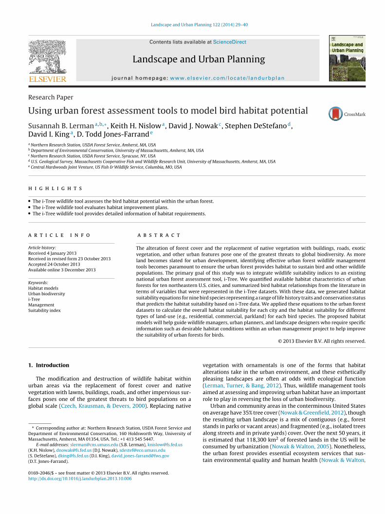
per 0.04 ha. The species relies on forested areas and we includedthree variables to describe these habitat needs. Adkins Giese andCuthbert (2003) observed 24 trees per 0.04 ha and a basal areaof 34 m2/ha in oak forests of the Upper Midwest, while Conner(1980) observed 30 trees/0.04 ha and a basal area of 14 m2/ha inoak-hickory forests around Blacksburg, VA. However, these stud-ies did not discern tree size. We wanted the model to reflectthe mean diameter of the cavity limb (21.6 cm; Jackson, 1976)so only included trees greater than 23 cm dbh and adjusted thedensities to reflect these conditions (Table 5). We fit a rationalfunction (0 − 0.0035 + (0.1606 × tree density))/(1 + (−0.1417 × treedensity) + (0.0233 × tree density2)) where tree density representsthe density of trees greater than 23 cm dbh within a 0.04 haplot, through these data points to predict how habitat suit-ability varied with large tree density (Fig. 1). We assumedsuitability was the lowest when trees were absent. Our inclu-sion of basal area for all trees greater than 6 cm dbh reflectsthe propensity for this species to prefer relatively dense forests(Shackelford, Brown, & Conner, 2000; Table 6). We fit a logisticfunction 0.9906/(1 + (47.9216 × exp(−0.9689 × basal area))) wherebasal area is m2/ha and calculated for all trees greater than 6 cmdbh, through these data points to quantify the relationship betweenbasal area and the SI score (Fig. 2).

Canopy coverage has the potential to predict habitat suit-ability. DeGraaf, Yamasaki, Leak, and Lester (2006) suggestedthat when canopy coverage exceeds 35%, the site providedsuitable conditions for red-bellied woodpeckers. We based ourassumed values for canopy cover on qualitative accounts andpersonal observations of the species in forested suburban and

riparian areas, with lack of observations in areas with little to nocanopy cover and areas with an extremely dense canopy cover(Table 7). We fit a rational function (−0.0371 + (0.0124 × percentcanopy))/(1 + (−0.0363 × percent canopy) + (0.0005 × percent

as follows: AMRO, American robin; BAOR, Baltimore oriole; BCCH, black-cappedBWO, red-bellied woodpecker; SCTA, scarlet tanager; WOTH, wood thrush. Models

on

9054 + (−0.0023519694 × x))/(1 + (−0.031238306 × x) + (0.00059471346 × x2))9182 + (−0.083072 × x) + (0.000538 × x2))35 × exp(0 − ((x − 35.4635207)2)/(2 × 15.35078892))7801 + (0.27942563 × x))/(1 + (−0.4470676 × x) + (0.13110269 × x))× exp((0 − ((x) − 63.568198)2)/1795)(1 + (32.567 × exp(−1.403x)))2/(1 + (11.742599 × exp(−0.48523169×)))

× exp((0 − ((x) − 63.568198)2)/1795)(1 + (32.567 × exp(−1.403x)))2/(1 + (11.742599 × exp(−0.48523169×)))035052 + (0.0148132 × x))/(1 + (−0.0378391 × x) + (0.00065325 × x2)) × −0.147 × (1.2498289 − exp(−2.42900485 × x))7/(1 + (40.643183849 × exp(−0.104376 × x)))93 + (−0.0879822662 × x))/(1 + (−0.3167288645 × x) + (0.0546857954 × x2))33686 + (−0.005359156 × x))/(1 + (−0.036974589 × x) + (0.0006728828 × x2))49075 + (0.021340335 × x))/(1 + (−0.02120201 × x) + (0.000432969 × x2))/(1 + (47.9216 × exp(−0.9689 × x)))71 + (0.0124 × x))/(1 + (−0.0335 × x) + (0.0005 × x2)) × −0.1

(15.67 × exp(−5.338 × x)))00347415 + (0.160609 × x))/(1 + (−0.141679 × x) + (0.0233308 × x2)) × −0.1/(1 + (49.295 × exp(−0.1088 × x)))5/(1 + (19,171.9801 × exp(−0.16936 × x)))009840608 × 4.3992415) + (1.6780139 × x0.25391))/(4.3992 + x0.2539122)2702/(1 + (24,569.22035 × exp(−0.6493929 × x)))(1 + (224.7853 × exp(−0.1081 × (x))))3/(1 + (141,241.64 × exp(−0.1531 × x)))1978/(1 + (65.800186 × exp(−0.758149 × (x)))))

ut will be incorporated into the i-Tree program, and analyzed when spatial data is

34 S.B. Lerman et al. / Landscape and Urban Planning 122 (2014) 29– 40

Table 4The suitability index (SI) scores for nine bird species in ten northeastern cities, for different urban land-uses. City SI score is the mean score per species and per city. Speciescodes as follows: AMRO, American robin; BAOR, Baltimore oriole; BCCH, black-capped chickadee; CACH, Carolina chickadee; EUST, European starling; NOCA, northerncardinal; RBWO, red-bellied woodpecker; SCTA, scarlet tanager; WOTH, wood thrush.

Land use City n AMRO BAOR CACH EUST NOCA RBWO SCTA WOTH MEAN

CITY SI SCORE Baltimore, MD 195 0.52 0.25 0.25 0.25 0.24 0.20 0.01 0.10 0.22Commercial Baltimore, MD 41 0.43 0.08 0.11 0.18 0.10 0.06 0.00 0.01 0.12Industrial Baltimore, MD 14 0.63 0.13 0.15 0.25 0.24 0.06 0.00 0.01 0.18Park Baltimore, MD 22 0.43 0.24 0.43 0.18 0.20 0.37 0.04 0.44 0.26Residential Baltimore, MD 90 0.57 0.33 0.26 0.35 0.32 0.22 0.01 0.06 0.27Transportation Baltimore, MD 16 0.45 0.23 0.32 0.09 0.16 0.29 0.03 0.15 0.20Vacant Baltimore, MD 5 0.51 0.49 0.26 0.07 0.55 0.26 0.00 0.02 0.24

CITY SI SCORE Boston, MA 220 0.49 0.29 0.27 0.19 0.21 0.26 0.01 0.06 0.21Commercial Boston, MA 13 0.63 0.26 0.31 0.38 0.22 0.26 0.01 0.09 0.25Industrial Boston, MA 23 0.51 0.26 0.21 0.25 0.20 0.16 0.01 0.02 0.20Park Boston, MA 35 0.60 0.28 0.25 0.27 0.14 0.27 0.01 0.06 0.22Residential Boston, MA 62 0.47 0.41 0.36 0.13 0.30 0.41 0.01 0.09 0.26Transportation Boston, MA 10 0.51 0.11 0.13 0.12 0.11 0.07 0.00 0.00 0.12Vacant Boston, MA 28 0.34 0.24 0.50 0.01 0.21 0.49 0.03 0.22 0.23

CITY SI SCORE Jersey City, NJ 230 0.47 0.11 0.15 0.18 0.16 0.04 0.00 0.01 0.14Commercial Jersey City, NJ 29 0.43 0.06 0.07 0.09 0.10 0.01 0.00 0.00 0.09Industrial Jersey City, NJ 4 0.39 0.05 0.06 0.01 0.08 0.01 0.00 0.00 0.07Park Jersey City, NJ 33 0.57 0.08 0.16 0.28 0.09 0.06 0.00 0.03 0.15Residential Jersey City, NJ 64 0.47 0.17 0.21 0.26 0.29 0.07 0.00 0.02 0.19Transportation Jersey City, NJ 25 0.46 0.08 0.16 0.06 0.10 0.02 0.00 0.00 0.10Vacant Jersey City, NJ 13 0.42 0.09 0.17 0.01 0.10 0.02 0.00 0.00 0.09

CITY SI SCORE Moorestown, NJ 206 0.49 0.17 0.33 0.21 0.47 0.32 0.03 0.17 0.28Commercial Moorestown, NJ 31 0.50 0.18 0.20 0.20 0.66 0.14 0.01 0.03 0.25Industrial Moorestown, NJ 4 0.56 0.09 0.11 0.17 0.66 0.02 0.00 0.00 0.22Park Moorestown, NJ 45 0.44 0.07 0.41 0.18 0.35 0.41 0.08 0.33 0.28Residential Moorestown, NJ 103 0.56 0.25 0.34 0.28 0.50 0.33 0.02 0.10 0.31Transportation Moorestown, NJ 1 0.81 0.05 0.06 0.41 0.63 0.01 0.00 0.00 0.28

CITY SI SCORE New York City 214 0.46 0.20 0.20 0.20 0.21 0.17 0.01 0.06 0.18Commercial New York City 6 0.84 0.20 0.13 0.42 0.22 0.05 0.00 0.00 0.21Industrial New York City 12 0.48 0.22 0.18 0.24 0.15 0.13 0.00 0.03 0.18Park New York City 33 0.45 0.13 0.26 0.17 0.19 0.29 0.02 0.13 0.19Residential New York City 76 0.50 0.35 0.25 0.32 0.28 0.27 0.01 0.03 0.26Vacant New York City 53 0.38 0.10 0.20 0.03 0.17 0.19 0.02 0.10 0.13

CITY SI SCORE Philadelphia, PA 213 0.42 0.19 0.48 0.25 0.22 0.39 0.03 0.21 0.26Commercial Philadelphia, PA 3 0.75 0.41 0.30 0.54 0.20 0.29 0.00 0.00 0.29Industrial Philadelphia, PA 19 0.49 0.14 0.25 0.34 0.14 0.17 0.00 0.05 0.19Park Philadelphia, PA 53 0.28 0.13 0.74 0.10 0.17 0.69 0.07 0.54 0.30Residential Philadelphia, PA 62 0.57 0.33 0.40 0.52 0.26 0.30 0.00 0.02 0.31Transportation Philadelphia, PA 10 0.44 0.17 0.20 0.08 0.24 0.09 0.00 0.00 0.14Vacant Philadelphia, PA 50 0.31 0.10 0.54 0.03 0.26 0.42 0.03 0.29 0.22

CITY SI SCORE Scranton, PA 191 0.50 0.20 0.25 0.23 0.23 0.22 0.01 0.16 0.22Commercial Scranton, PA 32 0.47 0.15 0.10 0.16 0.20 0.05 0.00 0.01 0.14Industrial Scranton, PA 11 0.49 0.15 0.10 0.19 0.15 0.04 0.00 0.00 0.14Park Scranton, PA 9 0.54 0.29 0.33 0.25 0.25 0.35 0.01 0.29 0.26Residential Scranton, PA 94 0.56 0.18 0.19 0.44 0.22 0.13 0.01 0.06 0.23Transportation Scranton, PA 13 0.44 0.16 0.16 0.05 0.18 0.10 0.00 0.03 0.13Vacant Scranton, PA 29 0.26 0.10 0.53 0.02 0.17 0.48 0.03 0.61 0.25

CITY SI SCORE Syracuse, NY 200 0.58 0.18 0.29 0.30 0.25 0.14 0.00 0.12 0.23Commercial Syracuse, NY 15 0.45 0.11 0.14 0.22 0.18 0.07 0.00 0.00 0.15Industrial Syracuse, NY 18 0.57 0.11 0.27 0.27 0.16 0.08 0.00 0.22 0.21Park Syracuse, NY 7 0.67 0.26 0.17 0.42 0.12 0.19 0.00 0.01 0.21Residential Syracuse, NY 113 0.64 0.20 0.24 0.38 0.26 0.12 0.00 0.03 0.24Transportation Syracuse, NY 9 0.50 0.13 0.22 0.07 0.51 0.04 0.00 0.01 0.17Vacant Syracuse, NY 30 0.40 0.11 0.50 0.10 0.17 0.21 0.01 0.46 0.23

CITY SI SCORE Washington, DC 201 0.50 0.31 0.26 0.23 0.22 0.31 0.07 0.06 0.23Commercial Washington, DC 10 0.43 0.15 0.12 0.17 0.21 0.09 0.00 0.00 0.15Industrial Washington, DC 7 0.46 0.19 0.10 0.16 0.21 0.08 0.00 0.00 0.15Park Washington, DC 53 0.46 0.24 0.33 0.15 0.24 0.41 0.17 0.15 0.24Residential Washington, DC 91 0.50 0.44 0.27 0.20 0.30 0.36 0.03 0.03 0.26

CITY SI SCORE Woodbridge, NJ 215 0.52 0.23 0.27 0.21 0.07 0.24 0.01 0.12 0.20Commercial Woodbridge, NJ 20 0.45 0.19 0.16 0.14 0.08 0.14 0.01 0.06 0.15Industrial Woodbridge, NJ 5 0.43 0.09 0.09 0.01 0.09 0.01 0.00 0.00 0.08Park Woodbridge, NJ 29 0.32 0.10 0.56 0.13 0.03 0.59 0.07 0.48 0.25Residential Woodbridge, NJ 98 0.64 0.35 0.27 0.32 0.08 0.24 0.01 0.04 0.24Transportation Woodbridge, NJ 22 0.50 0.11 0.13 0.13 0.08 0.04 0.00 0.05 0.12

S.B. Lerman et al. / Landscape and Urban Planning 122 (2014) 29– 40 35

Table 5Relationship between large tree density (trees larger than 23 cm dbh) per 0.04 haand suitability index (SI) for red-bellied woodpecker (RBWO) habitat, and associatedreferences.

Large tree density (per 0.04 ha) SI score (RBWO) Reference

0 0 Assumed value3 0.6 Assumed value6 1 Adkins Giese and

Cuthbert (2003)8 0.9 Conner (1980)

11 0.8 Assumed value

Fig. 1. Relationship between large tree density (trees larger than 23 cm dbh) per0.04 ha and suitability index (SI) for red-bellied woodpecker (RBWO) habitat, andassociated references.

Table 6Relationship between basal area (trees > 6 cm dbh) per ha and suitability index (SI)for red-bellied woodpecker (RBWO) habitat, and associated references.

Basal area (per ha) SI score (RBWO) Reference

0 0 Assumed value4 0.5 Assumed value8 0.95 Conner, 1980 (based on SD)

c0t(a

TRb

to quantify the relationship between trees with dead wood and theSI score (Fig. 4). We calculated the geometric mean of these habitatmodels to generate a final SI score for this species.

14 1 Conner, 198034 1 Adkins Giese and Cuthbert (2003)

anopy2)), where percent canopy represents the percent of a.04 ha plot with tree canopy cover, through these data points

o predict how habitat suitability varied with canopy coverageFig. 3). We assumed suitability was the lowest when trees werebsent.

able 7elationship between canopy percent per 0.04 ha and suitability index (SI) for red-ellied woodpecker (RBWO) habitat, and associated references.

Canopy percent (per 0.04 ha) SI score (RBWO) Reference

0 0 Assumed value15 0.1 Assumed value20 0.3 Assumed value25 0.5 Assumed value35 0.9 DeGraaf et al. (2006)62 1 Straus et al. (2011)

Fig. 2. Relationship between basal area (trees > 6 cm dbh) per ha and suitabilityindex (SI) for red-bellied woodpecker (RBWO) habitat, and associated references.

Although dead wood is necessary for foraging and nesting, it isnot essential for detecting red-bellied woodpeckers. Of 42 nests insouthwest Ontario, Straus, Bavrlic, Nol, Burke, and Elliott (2011)observed 93% of the nests in dead and declining trees and 6% ofnests in healthy trees. Adkins Giese and Cuthbert (2003) observedthree dead or declining trees per 0.04 ha in the Midwest (Table 8).We fit a logistic function 1/(1 + (15.67 × exp(−5.338 × dead wooddensity per 0.04 ha))) (where dead wood is recorded as trees witha condition of fair, poor, dying or dead) through these data points

Fig. 3. Relationship between canopy percent per 0.004 ha and suitability index (SI)for red-bellied woodpecker (RBWO) habitat, and associated references.

36 S.B. Lerman et al. / Landscape and Ur

Table 8Relationship between dead wood density per ha and suitability index (SI) for red-bellied woodpecker (RBWO) habitat, and associated references.

Dead wood density(per 0.04 ha)

SI score(RBWO)

Reference

0 0.06 Straus et al. (2011)1 0.93 Straus et al. (2011)3 1 Adkins Giese and Cuthbert (2003)

3

7albcbicrEtftbrdbwon(wpw

Fr

.3. Model validations

At the BES LTER sites, the American robin was recorded in2 of the 83 bird monitoring/i-Tree locations, Carolina chick-dee in 19 of the 83 locations, European starling in 62 of the 83ocations, northern cardinal in 60 of the 83 locations, and red-ellied woodpecker in 12 of the 83 locations. Spearman rankorrelation identified a significant and positive relationshipetween the HSI score and mean bird abundance at the BES LTER

-Tree locations for American robin (P = 0.0043, rs = 0.31), Carolinahickadee (P = 0.0011, rs = 0.3515), northern cardinal (P = 0.0022,s = 0.3311), red-bellied woodpecker (P = 0.0008, rs = 0.3596), anduropean starling (P = 0.0349, rs = 0.2333). When testing the sensi-ivity of the models by subsequently removing individual variablesrom whole models, we found no discrepancies between these par-ial and full models in their ability to predict mean bird abundanceetter than chance for Carolina chickadee, European starling anded-bellied woodpecker. The spearman rank correlation did notetect a significant relationship between the HSI score and meanird abundance in the American robin model when lawn percentas omitted (P = 0.5976, rs = 0.0593). However, when the model

mitted canopy cover and included lawn percent, we found a sig-ificant relationship between the HSI score and mean abundanceP = 0.0071, rs = 0.2950). Similarly, when the percent shrub coveras removed from the northern cardinal model, the model failed toredict presence when this species was recorded, though a modelith just percent shrubs was significant (P = 0.0140, r = 0.2705).

s

ig. 4. Relationship between deadwood density per ha and suitability index (SI) fored-bellied woodpecker (RBWO) habitat, and associated references.

ban Planning 122 (2014) 29– 40

3.4. Illustrating applications

For the most part, habitat suitability in Baltimore and Syracusedeclined from 2001 to 2009 (Table 9). Important resources suchas canopy cover in Baltimore declined by 33.8% in vacant lots, andlarge tree density in Syracuse declined by 0.8 and 3.4 trees in resi-dential and vacant lots between the two time periods (unpublishedi-Tree dataset). Habitat suitability scores significantly decreased forBaltimore oriole, northern cardinal, and red-bellied woodpeckerbetween 2001 and 2009 in Syracuse residential areas and vacantlots, and for scarlet tanagers in vacant lots only. Habitat suitabilityalso differed for red-bellied woodpecker in Baltimore residentialareas and for Carolina chickadee, red-bellied woodpecker, andwood thrush in Baltimore vacant lots. In contrast, habitat suitabil-ity increased for wood thrushes (Syracuse) and northern cardinals(Baltimore) in residential areas during this time period (Table 9).We failed to find a significant change in commercial, cemetery, golfcourse or institutional land-use plots in Baltimore and Syracuse.

4. Discussion

Integrating validated bird habitat suitability models into i-Treecan provide a more comprehensive assessment of the ecosys-tem services provided by the urban forest. Essentially, our modelstranslate the i-Tree raw data’s detailed information on the for-est composition and structure into relative assessments of habitatvalue for birds. The bird habitat models suggest which speciesspecifically, and guilds broadly, can be supported by an urban for-est. By selecting which bird models to focus on (e.g., native or rarespecies), other societal values can be included in this assessmentand guide general forest planning in urban areas. In addition, thebird habitat models have the capacity to provide specific targets(i.e., canopy percent or dead wood density) geared toward urbanforesters and planners when determining how to manage the urbanforest for wildlife.

Our validation efforts support the efficacy of using the habitatmodels to predict the habitat quality of urban areas for a variety ofspecies. Although we were unable to validate the Baltimore orioleand scarlet tanager model at this time, we agree with Brooks (1997)that these untested models still have greater value than no infor-mation about these species’ habitat relationships. In several cases,sensitivity analyses helped to identify particularly influential habi-tat parameters. For example, percent lawn for American robin andpercent shrub cover for northern cardinal have strong influences onthe habitat suitability for the respective species. Although the mod-els with insignificant results highlight the unequal effect of theseparticular variables, the models that included all the habitat vari-ables had a higher rank scores, suggesting the model had strongerpredictive power when these variables were included.

The i-Tree habitat models link habitat features with an SI scorereflecting the suitability of a site for that species. Each habitat vari-able has an optimal value for a particular species (i.e., when thesuitability index score is 1.0, the site has the greatest potential tosupport said species). Less than optimal values result in lower SIscores and provide a baseline for habitat improvement recommen-dations. Compared with the other cities, Jersey City had the lowestmean SI scores for all but one species (Table 3). The i-Tree programassessed canopy coverage at 13%, well below the national averageof 35.1% (Nowak & Greenfield, 2012). Eight species included canopypercent as an important limiting variable with optimal values ran-ging between 25% and 100% (Supplementary material).

Urban parks, vacant lots, and residential land-uses had high SIscores for most of the species modeled (Table 3), and species of con-servation concern in particular (Dettmers & Rosenberg, 2000). Forexample, urban parks and vacant lots had the highest SI score for

S.B. Lerman et al. / Landscape and Urban Planning 122 (2014) 29– 40 37

Table 9A comparison of suitability index (SI) scores for six bird species and mean values for two habitat variables at the same i-Tree monitoring plot in 2001 and 2009 in Syracuse,NY and Baltimore, MD for residential and vacant lot land-uses. The SI scores for American robin and European starling did not exhibit any significant changes. Species habitatmodels in commercial and institutional land-uses, and golf courses failed to show significant relationships.

Residential Vacant lot

2001 2009 F P 2001 2009 F P

BALTIMORE n = 87 n = 90 n = 18 n = 5American robin 0.54 0.57 1.22 0.27 0.39 0.51 1.62 0.22Baltimore oriole 0.35 0.33 0.09 0.75 0.35 0.49 0.58 0.45Carolina chickadee 0.3 0.26 1.34 0.25 0.65 0.26 5.28 0.032European starling 0.34 0.3 0.88 0.35 0.07 0.04 0.24 0.63Northern cardinala 0.35 0.33 0.47 0.49 0.22 0.55 16.71 0.0005Red-bellied woodpecker 0.34 0.24 4.28 0.04 0.66 0.26 5.53 0.029Scarlet tanager 0.01 0.01 0.97 0.33 0.1 0.01 2.05 0.17Wood thrush 0.03 0.06 2.19 0.14 0.3 0.14 3.30 0.084Tree canopy 25.31 24.74 0.02 0.88 52.22 18.4 5.50 0.03

SYRACUSE n = 117 n = 113 n = 33 n = 30American robin 0.61 0.64 1.24 0.27 0.37 0.4 0.27 0.6Baltimore oriole 0.46 0.22 46.37 <0.001 0.22 0.11 3.62 0.06Black-capped chickadee 0.23 0.27 2.64 0.11 0.48 0.5 0.03 0.86European starling 0.28 0.32 2.38 0.12 0.05 0.02 1.05 0.31Northern cardinal 0.39 0.29 11.92 0.0007 0.32 0.17 6.81 0.01Red-bellied woodpecker 0.24 0.16 7.57 0.0064 0.5 0.21 14.53 0.0003Scarlet tanager 0.01 0 0.42 0.52 0.07 0.01 5.24 0.026Wood thrusha 0.01 0.04 6.01 0.015 0.36 0.46 0.83 0.37Large tree density 1.16 0.39 24.88 <0.0001 3.85 0.4 22.46 <0.0001

sfrtwa2

pwaina2DTpSlwloarwwaocs

ofaeMtt

a An increase in suitability.

carlet tanager and wood thrush, suggesting that when managedor wildlife, these urban land-uses have the potential to supportare species. Residential land-uses had the highest SI score for Bal-imore oriole (Table 3) and although this land-use scored low forood thrush, the patterns suggest the existence of potential habitat

nd the conservation value of residential areas (Lerman & Warren,011).

The active management of dead wood in urban areas has theotential to stabilize populations for a guild that often adaptsell to cities (Chace & Walsh, 2006). Urban parks in Boston, MA

nd New York City had low SI scores compared to urban parksn Philadelphia, PA for red-bellied woodpecker, an obligate cavityester. Boston and New York also had low densities of dead wood,n important nesting resource for the species (Shackelford et al.,000). On average, Boston had 0.66 trees with dead wood (Deadens) per plot (6% of trees had some dead wood; unpublished i-ree dataset) and New York City had 0.85 trees with dead wooder plot (6% of trees had some dead wood; Nowak, Hoehn, Crane,tevens, & Walton, 2007). The model for dead wood density calcu-ated an SI score of 1 (i.e., most suitable) when at least three trees

ith dead wood were present in a 0.04 ha plot. The model calcu-ated an SI score of 0.93 with at least one tree with dead wood. Basedn the dead wood present, these two cities failed to reach a suit-bility threshold that had a high likelihood of supporting speciesequiring dead wood (i.e., areas with at least one tree with deadood) whereas Philadelphia, with an average nine trees per plotith dead wood (57% of all trees; unpublished i-Tree dataset), had

greater potential to support this species because of the presencef an important resource for cavity nesting species. Black-cappedhickadee, an additional species belonging to this nesting guild, hadimilar patterns.

The differences in dead wood densities might be the resultf different management regimes for these cities. Perhaps theormer two cities have a more active urban forestry departmentnd remove a greater degree of dead wood due to the hazards and

sthetics associated with dead and dying limbs (Harris, Clark, &atheny, 2004). Alternatively, the differences could also be due

o different tree population structures (e.g., age or size distribu-ion) among cities. By delineating a threshold of suitability for each

habitat variable, the models provide specific targets for improvingthe habitat conditions for a particular species, which is neces-sary for identifying management goals (Kroll & Haufler, 2006). Forexample, the city of New York had low scores for red-bellied wood-pecker, particularly in commercial and industrial land-uses. Basedon the habitat model description for this species (see model exam-ple), the optimal values for key habitat features are as follows: sixlarge trees (> 23 cm dbh) per 0.04 ha, 14 m2/ha basal area, 35–62%canopy coverage per 0.04 ha, and at least three trees with deadwood within 0.04 ha (Tables 1–4, respectively). Managers can thenreview the i-Tree data and assess how well the actual habitat val-ues accord with the optimal values. In New York City forest patches,the canopy percentage reached optimal values though the amountof deadwood fell below the threshold (unpublished i-Tree dataset).Thus incorporating management initiatives that encourage deadwood would improve the habitat conditions for this and other cav-ity nesting species. In sum, when cities or land-uses have low SIscores, the manager can pinpoint the sub-optimal variables anddevelop management plans that target these low scoring habitatfeatures.

Our example of how the i-Tree habitat module can documentSI changes over time demonstrated the potential for assessing theeffectiveness of management plans (or lack thereof). For example,in the Baltimore i-Tree dataset, we noted a sharp decline of treeswith dead wood between 2001 (3.59 trees per i-Tree plot) and2009 (0.73 trees per i-Tree plot). The deadwood density thresholdfor a suitable site for red-bellied woodpecker was three. There-fore this loss of deadwood might explain why the suitability indexfor species that rely on this resource also declined. An effectivemanagement strategy would include more selective criteria forremoving dead wood (e.g., only when posing a strong hazard risk),or perhaps encouraging the development and retention of snags inareas not frequented by people.

The models provide a substantial initial assessment of the habi-tat potential in the urban forest, while assisting decision makers

with the ultimate goal of improving urban bird habitat (Beaudryet al., 2010). Although the number of studies focusing on urbanbirds has increased over the past 20 years (Ramalho & Hobbs, 2012),and many of these studies included recommendations on how to

3 nd Ur

icttavati

tTttcetTtcta

mkapttfdtp&fasufota

niFs(dtmtirtan2thpaS

TW

8 S.B. Lerman et al. / Landscape a

mprove urban habitat, the recommendations are often for a spe-ific city (Lerman & Warren, 2011), and not necessarily accessibleo managers. The i-Tree tool was designed for urban managers andhus the wildlife component expands the capacity of the tool tollow for a more comprehensive assessment of the ecosystem ser-ices provided by the urban forest. With rapid habitat suitabilityssessment capabilities and ease of use for non-professional scien-ists, the wildlife component of i-Tree delivers a valuable tool thats applicable on a regional scale.

We recognize the importance of local and landscape fea-ures in limiting urban bird distribution (Chamberlain, Cannon, &oms, 2004; McCaffrey & Mannan, 2012). We did not have spa-ial locations available for the majority of the i-Tree plots andhus did not incorporate these landscape variables into the SIalculations. However, landscape variables are known to influ-nce the distribution for two of our modeled species: scarletanager and wood thrush (Hoover & Brittingham, 1998; Robinson,hompson, Donovan, Whitehead, & Faaborg, 1995). We describehese models based on landscape features (e.g., percent forestover within 1 km radius of i-Tree plot; Table 3), and will includehe models in the i-Tree program when spatial data are avail-ble.

Although currently limited to the local scale, the i-Tree habitatodels have the advantage of calculating SI for specific land-uses, a

nown feature that influences urban bird distribution (Blair, 1996),nd thus enabling managers to target low-scoring land-uses inde-endently. By discriminating among the land-use differences, theool recognizes the different jurisdictions and land ownership, andhe associated management strategies. For example, the strategyor increasing canopy coverage in city-owned open space mightiffer from residential lands, since the latter might require par-icipation from private households and the former might requireublic support for urban forestry programs (Warren, Ryan, Lerman,

Tooke, 2011). This local scale also provides greater opportunitiesor intervention. For example, mangers can affect canopy percent-ge through tree planting efforts but have little opportunity toignificantly increase the area of forest tracts embedded within therban matrix. Thus, although protecting large tracts of contiguousorest is essential for forest interior species (Robinson et al., 1995),nce the land becomes developed, there is little chance to effec-ively manage and incorporate management improvement planst this scale.

Similar to other habitat models, the i-Tree habitat models wereot as robust for generalist species compared with habitat special-

sts (Tirpak, Jones-Farrand, Thompson, Twedt, Baxter, et al., 2009).or example, the European starling, an urban exploiter (Blair, 1996),cored lower than expected for each city in all the urban land-usesTable 4), indicating that the ten cities used in the habitat modelemonstration supported few starlings. Based on personal observa-ions and the numerous studies documenting starlings as one of the

ost abundant urban birds (Chace & Walsh, 2006), we can assumehat the model did not accurately reflect starling habitat suitabil-ty. This was further supported during the validation process. Theesults from our models also suggested that variables other thanhose measured using i-Tree might better explain the habitat suit-bility of this ubiquitous species. Habitat specialists by their veryature are more restricted to a few key habitat features (Kilgo et al.,002). The i-Tree habitat models also had the tendency to overes-imate the suitability of potential habitat. The model calculated aigh likelihood of occupancy (>0.5) for more sites than will be occu-ied since the models did not account for interspecific competition,n additional factor that limits distribution (Fielding & Bell, 1997;

hochat et al., 2010).

Future directions include integrating these models into the i-ree program which involves coding the equations in i-Tree Eco.e plan to generate GIS range maps for each species to identify

ban Planning 122 (2014) 29– 40

the regions these equations should be activated (based on Breed-ing Bird Survey data). We plan to model additional species in otherregions, identify additional variables for the i-Tree data collectionprotocol that will help improve the estimation of the SI, and collectbird abundance data at i-Tree plots to further validate the models.We also urge future urban bird studies to adapt a habitat assess-ment protocol that includes the i-Tree variables and data collectionat the same spatial scale (0.04 ha). These studies will enable usto further model validation efforts as well as compare urban birdhabitats among cities.

The i-Tree habitat models provide a tool for local or regionalinitial assessments of the current state of the urban forest for pro-viding bird habitat. The assessment can be the basis for an extensiveand comprehensive conservation plan specifically geared towardurban land-uses. Results from this study will help guide urbanforesters, planners, and landscape designers who require specificinformation such as how many trees and shrubs are necessarywithin an urban greening project to reach conservation goals tar-geted at improving the suitability of urban bird habitat. Given thatmore than 80% of Americans live in urban environments (US Census,2012), it becomes imperative that urban forests provide opportu-nities for urban dwellers to connect with nature. This connectioncan improve and enhance health and well-being (Fuller, Irvine,Devine-Wright, Warren, & Gaston, 2007) while generating inter-est and support for conservation initiatives that aim to improveurban biodiversity (Miller, 2005).

Acknowledgments

We thank Bob Hoehn, Randy Dettmers, David Small, JamesSmith, Marshall Iliff, Frank Thompson, and Bill DeLuca for sup-plying the data and assistance with assessing the habitat models.Charlie Nilon and Paige Warren assisted with the bird data fromthe Baltimore Ecosystem Study (BES LTER) which is supported bythe National Science Foundation’s Long-term Ecological Researchprogram, grant number DEB 0423476. Bradley Blackwell, KirstenBryan, Adam Finkle and Sandra Haire, and three anonymousreviewers provided constructive comments on earlier drafts of themanuscript. S.B. Lerman was supported by a Switzer EnvironmentalLeadership grant from the Robert and Patricia Switzer Founda-tion.

Appendix A. Supplementary data

Supplementary data associated with this article can be found,in the online version, at http://dx.doi.org/10.1016/j.landurbplan.2013.10.006.

References

Adams, C. C. (1935). The relation of general ecology to human ecology. Ecology, 16(3),316–335.

Adkins Giese, C. L., & Cuthbert, F. J. (2003). Influence of surrounding vegetation onwoodpecker nest tree selection in oak forests of the Upper Midwest, USA. ForestEcology and Management 179, 523–534.

Akbari, H., Pomerantz, M., & Taha, H. (2001). Cool surfaces and shade trees to reduceenergy use and improve air quality in urban areas. Solar Energy, 70(3), 295–310.

Beaudry, F., Pidgeon, A. M., Radeloff, V. C., Howe, R. W., Mladenoff, D. J., & Bartelt, G. A.(2010). Modeling regional-scale habitat of forest birds when land managementguidelines are needed but information is limited. Biological Conservation, 143(7),1759–1769. http://dx.doi.org/10.1016/j.biocon.2010.04.025

Beissinger, S. R., & Osborne, D. R. (1982). Effects of urbanization on avian communityorganization. Condor, 84(1), 75–83.

Berlanga, H., Kennedy, J. A., Rich, T. D., Arizmendi, M. C., Beardmore, C. J., Blancher,P. J., et al. (2010). Saving our shared birds: Partners in flight tri-national vision for

landbird conservation. Ithaca, NY: Cornell Lab of Ornithology. Retrieved from:.http://www.savingoursharedbirds.org/final reports pdfs/PIF2010 EnglishFinal.pdf

Blair, R. B. (1996). Land use and avian species diversity along an urban gradient.Ecological Applications, 6(2), 506–519.

nd Urb

B

C

C

C

C

C

C

C

C

D

D

D

D

D

e

E

F

F

F

F

G

G

G

H

H

J

J

K

K

K

L

1307–1315.

S.B. Lerman et al. / Landscape a

rooks, R. P. (1997). Improving habitat suitability index models. Wildlife SocietyBulletin, 25(1), 163–167. http://dx.doi.org/10.2307/3783299

aro, T., & O’Doherty, G. (1999). On the use of surrogate species in con-servation biology. Conservation Biology, 13(4), 805–814. http://dx.doi.org/10.1046/j.1523-1739.1999.98338.x

hace, J. F., & Walsh, J. J. (2006). Urban effects on native avifauna: A review. Landscapeand Urban Planning, 74(1), 46–69.

hamberlain, D. E., Cannon, A. R., & Toms, M. P. (2004). Associations of gardenbirds with gradients in garden habitat and local habitat. Ecography, 27(5),589–600.

lergeau, P., Savard, J. P. L., Mennechez, G., & Falardeau, G. (1998). Bird abundanceand diversity along an urban-rural gradient: A comparative study between twocities on different continents. Condor, 100(3), 413–425.

onner, R. (1980). Foraging habits of woodpeckers in southwestern Virginia. Journalof Field Ornithology, 51(2), 119–127.

roci, S., Butet, A., & Clergeau, P. (2008). Does urbanization filter birds on the basisof their biological traits? Condor, 110(2), 223–240.

rooks, K. R., Suarez, A. V., & Bolger, D. T. (2004). Avian assemblages along a gradientof urbanization in a highly fragmented landscape. Biological Conservation, 115(3),451–462.

zech, B., Krausman, P. R., & Devers, P. K. (2000). Economic associations amongcauses of species endangerment in the United States. BioScience, 50(7),593–601.

eGraaf, R., Tilghman, N., & Anderson, S. (1985). Foraging guilds of North-Americanbirds. Environmental Management, 9(6), 493–536.

eGraaf, R. M., & Wentworth, J. M. (1986). Avian guild structure and habi-tat associations in suburban bird communities. Urban Ecology, 9(3/4),399–412.

eGraaf, R. M., Yamasaki, M., Leak, W. B., & Lester, A. M. (2006). Technical guide to for-est wildlife habitat management in New England. Burlington, Vermont: Universityof Vermont Press.

ettmers, R., & Rosenberg, K. V. (2000). Partners in Flight landbird conser-vation plan: physiographic area 9: Southern New England. Retrieved from:.http://www.partnersinflight.org/bcps/plan/pl 09 10.pdf

riscoll, C. T., Lambert, K. F., Chapin, F. S., III, Nowak, D. J., Spies, T. A., Swanson, F. J.,et al. (2012). Science and society: The role of long-term studies in environmentalstewardship. BioScience, 62(4), 354–366.

Bird. (2012). eBird: An online database of bird distribution and abundance [web appli-cation]. Ithaca, NY: eBird. Retrieved from:. http://www.ebird.org

mlen, J. T. (1974). Urban bird community in Tucson, Arizona – Derivation, structure,regulation. Condor, 76(2), 184–197.

ernandez-Juricic, E. (2000). Avifaunal use of wooded streets in an urbanlandscape. Conservation Biology, 14(2), 513–521. http://dx.doi.org/10.1046/j.1523-1739.2000.98600.x

ielding, A. H., & Bell, J. F. (1997). A review of methods for the assessment ofprediction errors in conservation presence/absence models. Environmental Con-servation, 24(1), 38–49.

itzgerald, J., Thogmartin, W. E., Dettmers, R., Jones, T., Rustay, C., Ruth, J. M., et al.(2009). Application of models to conservation planning for terrestrial birds inNorth America. In J. J. Millspaugh, & F. R. Thompson III (Eds.), Models for plan-ning wildlife conservation in large landscapes (pp. 593–624). Boston, MA, USA:Academic Press.

uller, R. A., Irvine, K. N., Devine-Wright, P., Warren, P. H., & Gaston, K. J. (2007).Psychological benefits of greenspace increase with biodiversity. Biology Letters,3(4), 390–394.

ering, J., & Blair, R. (1999). Predation on artificial bird nests along an urban gra-dient: Predatory risk or relaxation in urban environments? Ecography, 22(5),532–541.

oddard, M., Dougill, A., & Benton, T. (2010). Scaling up from gardens: Biodiversityconservation in urban environments. Trends in Ecology & Evolution, 25(2), 90–98.http://dx.doi.org/10.1016/j.tree.2009.07.016

rinnell, J. (1917). The niche-relationships of the California Thrasher. Auk, 34(4),427–433.

arris, R. W., Clark, J. R., & Matheny, N. P. (2004). Arboriculture: Integrated manage-ment of landscape trees, shrubs, and vines. Upper Saddle River: Prentice Hall.

oover, J. P., & Brittingham, M. C. (1998). Nest-site selection and nesting success ofwood thrushes. Wilson Bulletin, 110(3), 375–383.

ackson, J. A. (1976). A comparison of some aspects of the breeding ecologyof red-headed and red-bellied woodpeckers in Kansas. Condor, 78(1), 67–76.http://dx.doi.org/10.2307/1366917

ones-Farrand, D. T., Fearer, T. M., Thogmartin, W. E., Thompson, F. R. T., III, Nelson,M. D., & Tirpak, J. M. (2011). Comparison of statistical and theoretical habitatmodels for conservation planning: The benefit of ensemble prediction. EcologicalApplications, 21(6), 2269–2282. http://dx.doi.org/10.1890/10-1047.1

ilgo, J. C., Gartner, D. L., Chapman, B. R., Dunning, J. B., Jr., Franzreb, K. E., Gauthreaux,S. A., et al. (2002). A test of an expert-based bird-habitat relationship model inSouth Carolina. Wildlife Society Bulletin, 30(3), 783–793.

inzig, A. P., Warren, P., Martin, C., Hope, D., & Katti, M. (2005). The effects of humansocioeconomic status and cultural characteristics on urban patterns of biodiver-sity. Ecology and Society, 10(1).

roll, A. J., & Haufler, J. B. (2006). Development and evaluation of habitatmodels at multiple spatial scales: A case study with the dusky fly-

catcher. Forest Ecology and Management, 229(1–3), 161–169. http://dx.doi.org/10.1016/j.foreco.2006.03.026

ack, D. (1933). Habitat selection in birds. With special reference to the effects ofafforestation on the Breckland avifauna. Journal of Animal Ecology, 2(2), 239–262.

an Planning 122 (2014) 29– 40 39

Lerman, S. B., Turner, V. K., & Bang, C. (2012). Homeowner associations as avehicle for promoting native urban biodiversity. Ecology and Society, 17(4)http://dx.doi.org/10.5751/ES-05175-170445

Lerman, S. B., & Warren, P. S. (2011). The conservation value of res-idential yards: Linking birds and people. Ecological Applications, 21(4),1327–1339.

McCaffrey, R. E., & Mannan, R. W. (2012). How scale influences birds’ responses tohabitat features in urban residential areas. Landscape and Urban Planning, 105(3),274–280. http://dx.doi.org/10.1016/j.landurbplan.2011.12.022

McCune, B., & Grace, J. B. (2002). Analysis of ecological communities. Gleneden Beach,OR: MjM Software Design.

Melles, S. J. (2005). Urban birds diversity as an indicator of human social diversityand economic inequality in Vancouver, British Columbia. Urban Habitats, 3(1),25–48.

Miller, J. R. (2005). Biodiversity conservation and the extinction of experience. Trendsin Ecology & Evolution, 20(8), 430–434.

Miller, J. R., & Hobbs, R. J. (2002). Conservation where people live andwork. Conservation Biology, 16(2), 330–337. http://dx.doi.org/10.1046/j.1523-1739.2002.00420.x

Nilon, C. H., Warren, P. S., & Wolf, J. (2011). Baltimore birdscapestudy: Identifying habitat and land-cover variables for an urbanbird-monitoring project. Urban Habitats, 6. Retrieved from:.http://www.urbanhabitats.org/v06n01/baltimore full.html

Nowak, D. J., Crane, D. E., & Stevens, J. C. (2006). Air pollution removal by urbantrees and shrubs in the United States. Urban Forestry & Urban Greening, 4(3),115–123.

Nowak, D. J., Crane, D. E., Stevens, J. C., Hoehn, R. E., Walton, J. T., & Bond, J. (2008).A ground-based method of assessing urban forest structure and ecosystem ser-vices. Arboriculture and Urban Forestry, 34(6), 347–358.

Nowak, D. J., & Greenfield, E. J. (2012). Tree and impervious cover in the UnitedStates. Landscape and Urban Planning, 107(1), 21–30.

Nowak, D. J., Greenfield, E. J., Hoehn, R. E., & Lapoint, E. (2013). Carbon storageand sequestration by trees in urban and community areas of the United States.Environmental Pollution, 178, 229–236.

Nowak, D. J., Hirabayshi, S., Bodine, A., & Hoehn, R. (2013). Modeled PM2. 5 removalby trees in ten U.S. cities and associated health effects. Environmental Pollution,178, 395–402.

Nowak, D. J., Hoehn, R., Crane, D. E., Stevens, J. C., & Walton, J. T. (2007). Assessingurban forest effects and values: New York City’s urban forest. USDA ForestService, Northern Research Station Resource Bulletin NRS-9. Newtown Square:PA.

Nowak, D. J., & Walton, J. T. (2005). Projected urban growth (2000–2050) andits estimated impact on the US forest resource. Journal of Forestry, 103(8),383–389.

Ramalho, C. E., & Hobbs, R. J. (2012). Time for a change: Dynamic urbanecology. Trends in Ecology & Evolution, 27(3), 179–188. http://dx.doi.org/10.1016/j.tree.2011.10.008

Rich, T. D., Beardmore, C. J., Berlanga, H., Blancher, P. J., Bradstreet, M. S. W.,& Butcher, G. S. (2004). Partners in Flight North American landbird conserva-tion plan. Ithaca, NY: Cornell Lab of Ornithology. Retrieved from:. http://www.partnersinflight.org/cont plan/

Robinson, S. K., Thompson, F. R., III, Donovan, T. M., Whitehead, D. R., & Faaborg,J. (1995). Regional forest fragmentation and the nesting success of migratorybirds. Science, 267(5206), 1987.

Roloff, G. J., & Kernohan, B. J. (1999). Evaluating reliability of habitat suitability indexmodels. Wildlife Society Bulletin, 27(4), 973–985.

Shackelford, C. E., Brown, R. E., & Conner, R. N. (2000). Red-bellied wood-pecker (Melanerpes carolinus). In A. Poole (Ed.), The Birds of NorthAmerica Online http://dx.doi.org/10.2173/bna.500. Retrieved from:.http://bna.birds.cornell.edu/bna/species/500

Shanahan, D. F., Possingham, H. P., & Martin, T. G. (2011). Foraging heightand landscape context predict the relative abundance of bird species inurban vegetation patches. Austral Ecology, 36(8), 944–953. http://dx.doi.org/10.1111/j.1442-9993.2010.02225.x

Shochat, E., Lerman, S. B., Anderies, J. M., Warren, P. S., Faeth, S. H., & Nilon, C. H.(2010). Invasion, competition, and biodiversity loss in urban ecosystems. Bio-Science, 60(3), 199–208. http://dx.doi.org/10.1525/bio.2010.60.3.6

Simberloff, D., & Dayan, T. (1991). The guild concept and the structure of eco-logical communities. Annual Review of Ecology and Systematics, 22, 115–143.http://dx.doi.org/10.1146/annurev.ecolsys.22.1.115

Sherry, T. W., & Holmes, R. T. (1985). Dispersion patterns and habitat responses ofbirds in northern hardwoods forests. In M. L. Cody (Ed.), Habitat selection in birds(pp. 283–309). Orlando: Academic Press.

Straus, M. A., Bavrlic, K., Nol, E., Burke, D. M., & Elliott, K. A. (2011). Reproductivesuccess of cavity-nesting birds in partially harvested woodlots. Canadian Journalof Forest Research, 41(5), 1004–1017. http://dx.doi.org/10.1139/X11-012

Strohbach, M. W., Haase, D., & Kabisch, N. (2009). Birds and the city: Urban biodi-versity, land use, and socioeconomics. Ecology and Society, 14(2).

Tirpak, J. M., Jones-Farrand, D., Thompson, F. R., III, Twedt, D. J., Baxter, C. K.,Fitzgerald, J. A., et al. (2009). Assessing ecoregional-scale habitat suitabilityindex models for priority landbirds. Journal of Wildlife Management, 73(8),

Tirpak, J. M., Jones-Farrand, D. T., Thompson, F. R., III, Twedt, D. J., & Uihlein, W.B., III. (2009). Multiscale habitat suitability index models for priority landbirdsin the Central Hardwoods and West Gulf Coastal Plain/Ouachitas Bird Conser-vation Regions (General Technical Report NRS-49). Newtown Square, PA: U.S.

4 nd Ur

U

U

urban gradients in Massachusetts. Landscape and Urban Planning, 102(2), 82–92.

0 S.B. Lerman et al. / Landscape a

Department of Agriculture, Forest Service, Northern Research Station, USA.Retrieved from:. http://www.nrs.fs.fed.us/pubs/9723i

.S. Census Bureau. (2012). Growth in urban populations outpaces rest of nation,

Census Bureau reports. Retrieved from:. http://www.census.gov/newsroom/releases/archives/2010 census/cb12-50.html

.S. Fish and Wildlife Service. (2012). Urban conservation treaty formigratory birds. Retrieved from:. http://www.fws.gov/migratorybirds/Partnerships/UrbanTreaty/urbantreaty.html

ban Planning 122 (2014) 29– 40

Warren, P. S., Ryan, R. L., Lerman, S. B., & Tooke, K. A. (2011). Social and insti-tutional factors associated with land use and forest conservation along two

http://dx.doi.org/10.1016/j.landurbplan.2011.03.012Watts, B. D. (1999). Partners in flight: Mid-Atlantic Coastal Plain bird con-

servation plan: physiographic Area #44. Retrieved from:. http://www.partnersinflight.org/bcps/plan/pl 44 10.pdf