Landmark-Based Geometric Morphometrics: What Fish Shapes Can Tell Us about Fish Evolutioncondor.depaul.edu/waguirre/park_et_al_13.pdf · 2014-03-27 · Shapes Can Tell Us about Fish

Tested Studies for Laboratory TeachingProceedings of the Association for Biology Laboratory EducationVol. 34, 361-371, 2013

361

Landmark-Based Geometric Morphometrics: What Fish Shapes Can Tell Us about Fish EvolutionPeter J. Park1, Windsor E. Aguirre2, Deborah A. Spikes3 and Joan M. Miyazaki3

1 Nyack College, Department of Biology and Chemistry, 1 South Blvd., Nyack NY 10960 USA2 DePaul University, Department of Biological Sciences, 2325 North Clifton Ave, Chicago IL 60614 USA3 Stony Brook University, Department of Undergraduate Biology, Stony Brook NY 11794 USA ([email protected], [email protected], [email protected],

[email protected])

Students learn how to apply landmark-based geometric morphmetric techniques to compare lake samples of the threespine stickleback fish (Gasterosteus aculeatus) from Cook Inlet, Alaska. The stickleback is an excellent model organism to teach natural selection, adaptation, and speciation. It is ancestrally a marine or sea-run fish. In-numerable freshwater populations have evolved from these sea-run forms and exhibit specializations to freshwater habitats that range from shallow, structurally complex lakes with benthic-foraging stickleback, to deeper, structur-ally simple lakes with open-water planktivorous stickleback. Body shapes of benthic and planktivore stickleback are analyzed using free Tps-series software. Landmark digitization and shape analysis are emphasized.

Firstpage36Keywords: threespine stickleback, morphometrics, body shape, foraging morphology

Link to Supplemental Materials

http://www.ableweb.org/volumes/vol-34/park/supplement.htm

© 2013 by Nyack College

Morphometrics is the study of size and shape of living organisms, which has traditionally been accomplished us-ing linear measures (e.g., lengths, widths), masses, angles, ratios, and areas. A more sophisticated yet readily accessible method available to biologists is landmark-based geometric morphometrics, in which data can be collected in the form of spatial arrangements of landmarks along a biological structure. This powerful technique can capture differences in structures that are not easily observed through traditional types of measurements or by the naked eye. Students can benefit from an application of landmark-based geometric morphometrics because these techniques are current state-of-the-art tools, and biological shapes are intrinsically interest-ing and ecologically informative. In this laboratory, students will apply landmark-based geometric morphometrics to in-vestigate ecologically-dependent population differences of body shapes in a well-studied evolutionary model organism - the threespine stickleback fish (Gasterosteus aculeatus). Evolutionary changes in body shape can occur for a variety of reasons, but those of bottom-dwelling versus open-water stickleback populations are well-understood (Walker, 1997;

Aguirre, 2009). The same ecological dichotomy can be ex-tended to explain drastic body shape differences at higher taxonomic levels in a wide range of distantly-related fish taxa. Threespine stickleback exhibit an enormous range of vari-ation and has adapted to a variety of ecological conditions, making it a powerful evolutionary model organism (Gibson, 2005; Bell and Foster, 1994; Östlund-Nilsson et al., 2007). Sticklebacks are found along almost every coastline in the northern hemisphere and occur in three forms - marine, sea-run, and freshwater (Bell and Foster, 1994). They are ances-trally marine or sea-run and have colonized an immense ar-ray of post-glacial lakes. The lake populations studied in this laboratory occur in a region of south-central Alaska that was covered by glaciers less than 20,000 years ago (Bell et al., 2003), and thus, they must have been founded by sea-run an-cestors since then. The countless number of recently derived lake populations can be treated, in many cases, as natural, independently-derived replicate experiments. Furthermore, living sea-run populations still exist and can be used to infer the ancestral condition of any trait.

IntroductionPage 1 Spacer

mailto:peter.park%40nyack.edu?subject=

mailto:waguirre%40depaul.edu?subject=

mailto:deborah.spikes%40stonybrook.edu?subject=

mailto:joan.miyazaki%40stonybrook.edu?subject=

http://www.ableweb.org/volumes/vol-34/park/supplement.htm

362 Tested Studies for Laboratory Teaching

Park, Aguirre, Spikes and Miyazaki

Student OutlineBody Shapes and Their Ecological Correlates

The purpose of this exercise is to investigate the relationship between body shape variation, ecology, and evolution. How do you measure biological shapes and why are they important? In many fishes, body shape is closely associated with habitat type. For example, compare the tautog (Tautoga onitis) with the great barracuda (Sphyraena barracuda) (Fig. 1). These are two marine species commonly found along the eastern United States coast. How do these fishes differ in body shape? How would you quantify these differences? What ecological functions do their body shapes serve? Is the body shape of each fish species an adaptation to its native habitat?

Figure 1. Comparison of tautog and great barracuda. Scale bar is 5 cm. Images courtesy of Michael P. Kroessig.

One way to answer these questions is to study a model species that exhibits the natural variation that we seek to understand. In this laboratory, you will be introduced to the threespine stickleback fish (G. aculeatus). One of the best studied ecological dichotomies of threespine stickleback is the benthic-planktivore dichotomy, and an understanding of this dichotomy will help you better understand why the body shapes of fish like tautog and great barracuda differ. Unlike among-species differences, the differences between benthic (bottom-feeding) and planktivore (open-water foraging on plankton) stickleback occur at the level of different populations within a single species. The threespine stickleback is primitively marine or sea-run but has repeatedly colonized and adapted to diverse freshwater habitats, especially lakes (Bell, 1995). Adaptation to different foraging demands has resulted in predictable ecological and morphological divergence among stickleback lake populations. Benthic and plankti-vore stickleback populations represent extremes along a dietary continuum (McPhail, 1984, 1994). Benthic stickleback prey on relatively large invertebrates on structurally complex, shallow lake bottoms, but planktivore populations feed on small plankton in open waters.

Figure 2. Threespine stickleback (G. aculeatus) benthic and planktivore ecological dichotomy. Sea-runstickleback (top) are ancestral to lake populations. On opposite ends of an ecological continuum are shallow lakes and deep lakes. Stickleback in each type of habitat have adapted to the conditions of their lakes as is evident by their contrasting morphologies.

Proceedings of the Association for Biology Laboratory Education, Volume 34, 2013 363

Mini Workshop: Stickleback body shape evolution

Observe Fig. 2. How do you think benthic and planktivore stickleback differ? What are some reasonable explanations for these differences? How can you measure these differences? These are the very sorts of questions you will address in this labo-ratory. We will focus on body shape differences. Geometric morphometrics using landmark data can be used to quantify and analyze body shape differences, if they exist. You will learn to turn body shapes into numbers that can be used to statistically test for population differences. Shape data will be collected and analyzed from two stickleback lake populations. You will need to determine if both populations are benthics, both are planktivores, or if one is a benthic and the other is planktivore. Data col-lection and analysis will be achieved using free available software developed by Dr. F. James Rohlf from the Dept. of Ecology and Evolution at Stony Brook University.

Methods

Preparation

Identify the following files on your computer’s desktop:A. “SAMPLES” folder contains two sub-folders, each named after a specific Alaskan lake and includes digital images of ≥

20 fish specimens from that lake. These fish are stained with Alizarin Red S, a dye that makes their bones appear red.

B. “TPS PROGRAMS” folder contains three software programs that you will be using for setup, data collection, and data analysis. Tps_Utility program will be used to create an input file that the data acquisition program, Tps_Digitize, can read. Tps_Digitize will retrieve the images and allow you to digitize landmarks on them. Tps_Relative Warps program will be used to generate a summary of your data. Each program begins with the same prefix “Tps” because it is short for “Thin-plate spline,” which is a fancy way of saying thin metal sheet. These programs will allow you to visualize 2-D shape differences of your specimens based on deformation of the average shape of all specimens; this average shape is also called the consensus (or reference) shape. To better understand what the software is doing, you can think of the reference shape as occupying a thin flat sheet of metal (Fig. 3). Individual shapes of actual specimens can be described/re-created by bending the metal sheet occupied by the reference shape. Basically, you twist and turn the reference shape until you arrive at the shape that best matches each specimen. Theoretically, the flat reference sheet can be bent in many different ways to generate a desired final shape, but the program automatically chooses the final sheet configuration achieved by using the least amount of “bending energy” (or the physical energy needed to bend the reference sheet to a desired shape). Thus, these programs employ a physics model (i.e., the bending of a thin metal sheet) to summarize biological shape differences (i.e., differences in body shapes). Finally, Microsoft® Excel (not a part of the Tps-software series) can be used to customize the presentation of your data or to apply simple statistical tests.

Figure 3. Re-construction of specimens using Tps_Relative Warps. Program uses a physics model of a virtual thin metal sheet which is deformed to re-create specimen shapes and construct a shape space.



Protocols

Protocol 1: Setting up the data file

1. Each student should be prepared to position 15 landmarks on each specimen.

2. On your computer’s desktop, locate the “SAMPLES” folder containing fish images from Long Lake and Mud Lake. Browse through these images. You will notice that each photograph includes a small ruler. This is because photographs may have been taken at different magnifications, and the ruler can be used to size-scale the software if size measurements are desired. Why is size-scaling necessary before taking measurements?

3. Creating the input file. To get started, you will need to construct an input file from one of your lake population folders. This is done so that the data acquisition software can later recognize the images and allow you to record landmark data.

4. The input file can be created automatically using the Tps_Utility program. This program provides logistical functions. Open the Tps_Utility program. Go to “Operation” g ”Build tps file from images.” Start with the Long Lake folder located within the “SAMPLES” folder. Click on “Input,” and open this directory, highlight any one file, and then select “Open” (NOTE: The selection here is for only one arbitrary image file because this program is interested in the folder; the program automatically will find all the images from the desired folder once any single image is selected from it.). Click on “Output” and create a file name for the input file (e.g., LONG LAKE_INPUT.tps). Next, click on “Setup.” You can choose content of the file here. Choose “Select All” to include all images. Finally, click “Create” which will automati-cally generate the input file in your folder of images.

5. Repeat step 4 for the Mud Lake sample.

Protocol 2: Collecting landmark data

1. Next, you will use the input file that you created to collect landmark data. Open the Tps_Digitize program and upload one input file. Again, you can start with Long Lake fish. The input file should be located in the same folder as the specimen images (NOTE: if your input file is not in the same folder as the images to which it refers, you will get an error message).

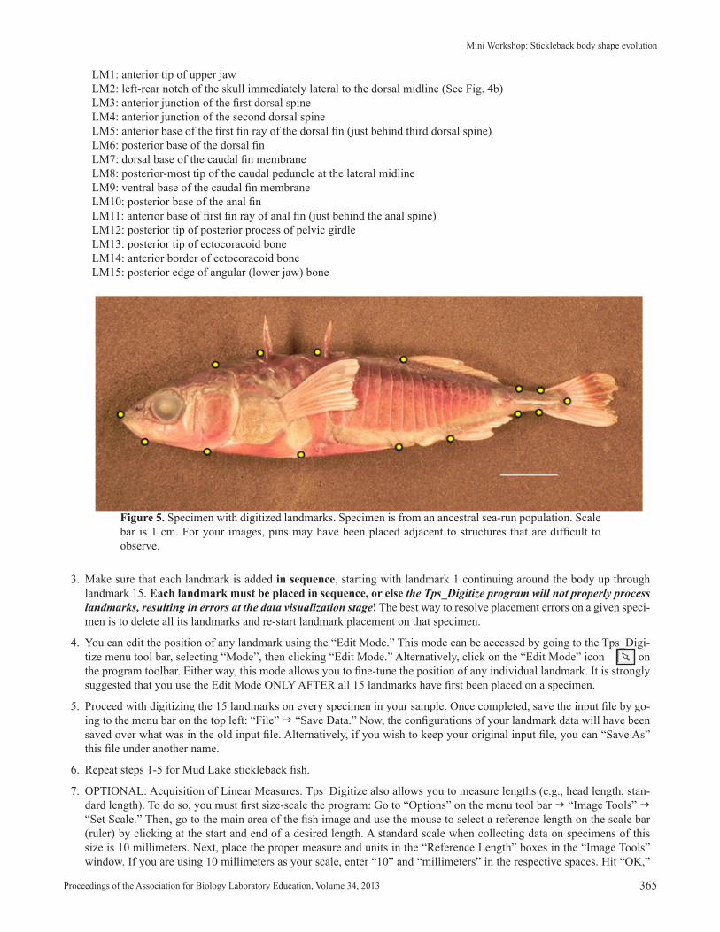
2. Click on the “Digitize landmarks” symbol located on the Tps_Digitize software toolbar. This mode allows you to place landmarks on the specimen. Place landmarks on the 15 positions marked in Fig. 4. To minimize variation across specimens due to random error, corresponding landmarks must be placed on the same positions for each specimen (See Fig. 5).

Figure 4. (a) Arrangement of landmarks. Lateral image of stickleback fish with landmarks. Major anatomical features are denoted in blue text. Scale bar is 10 mm. Modified from Aguirre, 2009. (b)Landmark 2. Position of LM2 is the circle, denoted by arrow. Dorsal aspect of skull, anterior to left. Scale bar is 5mm.

A B



Figure 5. Specimen with digitized landmarks. Specimen is from an ancestral sea-run population. Scale bar is 1 cm. For your images, pins may have been placed adjacent to structures that are difficult to observe.

3. Make sure that each landmark is added in sequence, starting with landmark 1 continuing around the body up through landmark 15. Each landmark must be placed in sequence, or else the Tps_Digitize program will not properly process landmarks, resulting in errors at the data visualization stage! The best way to resolve placement errors on a given speci-men is to delete all its landmarks and re-start landmark placement on that specimen.

4. You can edit the position of any landmark using the “Edit Mode.” This mode can be accessed by going to the Tps_Digi-tize menu tool bar, selecting “Mode”, then clicking “Edit Mode.” Alternatively, click on the “Edit Mode” icon onon on the program toolbar. Either way, this mode allows you to fine-tune the position of any individual landmark. It is strongly suggested that you use the Edit Mode ONLY AFTER all 15 landmarks have first been placed on a specimen.

5. Proceed with digitizing the 15 landmarks on every specimen in your sample. Once completed, save the input file by go-ing to the menu bar on the top left: “File” g “Save Data.” Now, the configurations of your landmark data will have been saved over what was in the old input file. Alternatively, if you wish to keep your original input file, you can “Save As” this file under another name.

6. Repeat steps 1-5 for Mud Lake stickleback fish.

7. OPTIONAL: Acquisition of Linear Measures. Tps_Digitize also allows you to measure lengths (e.g., head length, stan-dard length). To do so, you must first size-scale the program: Go to “Options” on the menu tool bar g “Image Tools” g “Set Scale.” Then, go to the main area of the fish image and use the mouse to select a reference length on the scale bar (ruler) by clicking at the start and end of a desired length. A standard scale when collecting data on specimens of this size is 10 millimeters. Next, place the proper measure and units in the “Reference Length” boxes in the “Image Tools” window. If you are using 10 millimeters as your scale, enter “10” and “millimeters” in the respective spaces. Hit “OK,”

LM1: anterior tip of upper jaw LM2: left-rear notch of the skull immediately lateral to the dorsal midline (See Fig. 4b) LM3: anterior junction of the first dorsal spine LM4: anterior junction of the second dorsal spine LM5: anterior base of the first fin ray of the dorsal fin (just behind third dorsal spine) LM6: posterior base of the dorsal fin LM7: dorsal base of the caudal fin membrane LM8: posterior-most tip of the caudal peduncle at the lateral midline LM9: ventral base of the caudal fin membrane LM10: posterior base of the anal fin LM11: anterior base of first fin ray of anal fin (just behind the anal spine) LM12: posterior tip of posterior process of pelvic girdle LM13: posterior tip of ectocoracoid bone LM14: anterior border of ectocoracoid bone LM15: posterior edge of angular (lower jaw) bone



and your image will be size-scaled. You must size-scale each image separately because each specimen could have been photographed at a different magnification.

Now, you are able to make linear measures (e.g., widths, lengths) on the fish. Go to “Modes” on the menu tool bar g “Mea-sure Mode.” (Before proceeding, check your scale by measuring the ruler itself!) A standard linear size measure for fish is standard length, which is the length from the tip of the upper snout to the end of caudal peduncle (i.e., linear distance between landmarks 1 and 8). Why do you think scientists measure only to the base of the tail region and not include the whole caudal fin? It is because often in the wild, fish may have parts of their caudal fin missing due to various reasons (e.g., predator evasion attempt, intraspecific aggression), and so the actual tip of the caudal fin becomes an unreliable marker if your goal is to get standard measurements from fish to fish; fish with parts of their caudal fin cut will not provide adequate data! Click the start and end of a desired length. As long as you size-scaled correctly for each specimen, you will see a length measurement in the designated units in the bottom-left corner of the image border. Record these values in your notebook as you collect the data. Length measures can be compared to area measurements calculated by other programs such as ImageJ or SigmaScan. Tps_Relative Warps program can also calculate centroid size (i.e., a geometric measure of size) for each speci-men (see Notes to the Instructor).

Protocol 3: Merging Your Two Input Files (Set-up for Tps_Relative Warps)

1. You have just collected data from two different stickleback lake samples. The two new input files need to be appended into one file so that the shape analysis software can process both samples simultaneously.

2. Create a new subfolder in your “SAMPLES” folder and name it “[Your last name] Data Analysis.” Place the two land-mark-digitized input files into the new folder. Remember, there are two input files- one from Long Lake and the other from Mud Lake.

3. Open the Tps_Utility program. Go to “Operation” g “Append files.” Click on “Input” and locate the new folder that you just created. Simply highlight any one file that appears within this folder. Click on “Output” and give a name to the appended digitized input file (e.g., LONG AND MUD_DIG_DATA.tps). Next, click on “Setup.” Select the digitized input file from Long Lake and from Mud Lake. Finally, choose “Create,” which will automatically generate the single appended file in your new Data Analysis folder.

Protocol 4: Shape Analysis of Stickleback Body Shapes

1. Now that all of your specimens are digitized and the landmark data are merged into one file, you can proceed to shape visualization and analysis. Open the Tps_Relative Warps program, which aligns all of your specimen shapes to create an average shape (the reference shape). The alignment corrects for differences in where the specimens are placed in the pictures, how they are rotated in the picture, and for differences in size among specimens. It then applies a physics model (i.e., the bending of a thin metal sheet) to help explain the shape differences among specimens. The shapes of the individual specimens are re-constructed by way of a mathematical algorithm that minimizes the amount of energy that was needed to bend the reference shape. The algorithm quantifies shapes and also creates a summary plot of all shapes in your dataset. This plot is called a shape space (or “morphospace”), and it estimates a range of possible shapes based on the model (See Fig. 3).

2. For shape data visualization, click on “Data” g select the appended file with digitized specimens from both populations (e.g. LONG AND MUD_DIG_DATA.tps). Next, click on “Consensus” g “Partial Warps” g “Relative Warps.”

The Consensus image is the average (reference) body shape of all your specimens combined.

Partial Warps- Raw landmark data get converted into new “shape variables.” See help menu in Tps_Relative Warps program or Zelditch et al. 2004 for more information.

Relative Warps- Conducts a Principal Components Analysis (PCA) and gives you a 2-D plot that displays the major axes of body shape variation in your dataset. PCA is a general multivariate method used to simplify complex data sets. To put it simply, this program uses the new shape variables to create the shape space. The X and Y-axes represent axes of varia-tion, and each data point represents the location of a specimen in that shape space.

3. It is possible to summarize the shape differences in the shape space by observing the shape variation across each axis. The best way to achieve this is to observe the shapes at the ends of the X-axis and the Y-axis. (Make sure that X:1 and Y:2 on the menu bar, which denotes that Principal Component (PC) 1 is the X axis and PC 2 is the Y axis. PC1 and PC2 are the axes that account for the greatest amount of body shape variation). Select the camera icon loca located on the menu toolbar. This option will allow you to visualize any one point within the shape space. For now, move the red circle



over the ends of the X-axis. Start at the most positive end (right tip of the horizontal line). Next, look at the shape at the

in your mind, morph these shapes into each other. This shape change is what the X-axis represents. If it helps, you can also select the movie camera icon from the menu toolbar to view the two points on the plot as a slide show. Repeat these steps for the Y-axis. By visualizing the X- and Y-axes in this way, you can get a quick preview of the major axes of shape

.

Figure 6. (a) Unedited PCA of body shapes. Shape space plot generated by Tps_Relative Warps using a sample of ten specimens. Each circle is the body shape of a specimen. (b) Edited PCA of body shapes. Shape space plot generated with Microsoft® Excel using data saved from Tps_Relative Warps. Each symbol in the plot denotes a specimen. ◊ (blue), Long Lake; X (red), Mud Lake. PC indicates Principal Component and the percentages in the axis labels indicate the amount of variation accounted for by each axis.

(a)

4. You can label each data point. Go to “Options” g “Option” g check the box for “Label Points.” This will allow you

5. If you desire, you can save the Relative Warps (=Principal Components Analysis) plot. Go to “File” g “Save plot…” and name it appropriately.

6. OPTIONAL: Customizing Your Plot. There are ways to make these plots more aesthetically pleasing. For example, you can take the raw values from your shape analysis plot and transfer them to Microsoft® Excel, which offers additional

g “Save” g “Save

-tion, which are those that you already observed from the Tps_Relative Warps program. You can re-create the scatterplot from Tps_Relative Warps in Excel using these two columns of data. With Excel, you can then partition the samples using colors and/or symbols. It is essential that the axes are in the same units because each axis refers to the same type of mea-

the terminal ends of each axis. See Fig. 6b.

(b)



The Big Picture

Benthic and planktivore stickleback are extremely divergent for foraging behavior and morphology, making each ecologi-cal type well-adapted to their natural habitat (See Schluter, 2000, Gow et al., 2007). Compared to benthics, planktivores have longer, narrower snouts (for feeding efficiently on small plankton, Willacker et al., 2010), more and longer bony finger-like pro-jections on the gill arches called gill rakers (for sieving small plankton efficiently during feeding, McPhail, 1984, 1992,1994; McKinnon and Rundle, 2002), more teeth (for chewing small plankton prey, Caldecutt et al., 2001), and a more elongate, streamlined body (for cruising long distances efficiently, Lavin and McPhail, 1985, 1986; Walker, 1997; Aguirre, 2009). We can use the results and knowledge about stickleback to better understand broader aspects of the biology of body shape evolution in other animals. To determine if the pattern we found with one benthic and one planktivore population can be gener-alized to other stickleback populations, one must study many more populations. Researchers have done this for a large number of stickleback populations and found that our result indeed can be generalized to other benthic and planktivore stickleback populations (Walker, 1998; Aguirre, 2009; Aguirre and Bell, 2012; Park and Aguirre, unpub. data). In fishes, body shape differences are often indicative of adaptation to specific ecological variables and can be used as a diagnostic of a species. An ecological pattern that is virtually identical to that of the benthic versus planktivore stickleback dichotomy is the among-species differences of benthic and pelagic species. Refer back to the comparison of the tautog and great barracuda. Like a planktivore stickleback, the barracuda is an open-water predator. It cruises the ocean in search of food (i.e., small fishes) much like pelagic sharks and sailfish. The barracuda body is built to glide and cut through the water without it having to expend too much energy. In contrast, the tautog is a structure-oriented fish just like a benthic stickleback, and its body shape reflects a territorial, bottom-dwelling lifestyle. Tautog are deep-bodied and muscular, and consequently, are built to maneuver efficiently in and out of their structurally complex territories. Tautog are also specialist predators that feed off the bottom on crustaceans and mollusks. Thus, knowledge of a single species, the threespine stickleback, provides valuable insight into the macroevolutionary diversification of major distantly-related fish groups.



Principal Components Analysis with Shapes.

Tps_Relative Warps generates a Principal Components Anal-ysis (PCA) of the shape data. PCA is a popular multivariate visualization technique. Interested readers should see Lattin et al. 2003. In brief, when PCA is applied to landmark data, each landmark is treated as an independent variable, and the Tps_Relative Warps program summarizes variation contrib-uted by all the landmarks simultaneously as best possible. In our lab activity, there were 15 landmarks used, which means there are theoretically 30 axes of variation (or dimensions) with which to summarize variation from our data. The num-ber of dimensions is double the number of landmarks used because each landmark has two coordinates on the 2-D plane of a photograph – an x and y coordinate. Actually, the num-ber of dimensions gets reduced further in the final PCA to 26 because the Tps_Relative Warps program eliminates four degrees of freedom (d.f.) as a consequence of translation (2 d.f.), scale (1 d.f.), and rotation (1 d.f.) when preparing the PCA. Thus, there are actually 26 independent axes or dimensions of variation from our data. However, visualiz-ing variation along 26 dimensions would be very difficult. Principal Components Analysis allows us to summarize the major patterns of variation along a few (two or three) axes that account for as much of the variation in the original data set as possible. PCA works in such a way that PC 1 is the axis that always accounts for the greatest amount of varia-tion in the data. PC 2 accounts for the second-most amount of variation with the constraint that it is orthogonal (at a right angle) to PC 1, and so on. How is it possible then that we can adequately explain our data with just two of the pos-sible 26 dimensions? While there is no set standard, many researchers will use the first two axes of variation to sum-marize their data variation if they cumulatively account for a large amount of the variation (e.g., >50%). Our first two axes account for ~60% of the variation (See LONG AND MUD_DIG_REPORT.txt). In support of our decision to use only the first two axes to summarize our shape data, visual inspection of the digitized specimen shapes in the PCA cor-respond very well with what the actual body shapes look like in their photographs. Thus in our case, the remaining 24 un-explained axes of variation can be set aside. For more on these advanced topics, see Zelditch et al. 2004.

Calculating Body Centroid Size.

Centroid size is a geometric measure of size that can be cal-culated for each specimen to take shape variation into ac-count. The alignment procedure scales all specimens to the same size but does not account for allometric shape varia-tion (variation in shape related to size). For example, even if you scale a human baby and adult to the same size, they will differ tremendously in shape because body shape changes substantially as humans grow. The same happens in other organisms including fish. Mathematically, centroid size is the square-root of the sum of squared distances of each land-mark from the midpoint of all landmarks used on a speci-

Notes for the Instructor This laboratory activity can be implemented to cover speciation, natural selection, adaptation, ecological diversi-fication, niche, microevolution, macroevolution, and trophic morphology.

Documents, Images, and Data Available for Download.

The following folders with files are made available on the ABLE server.

(1) “SAMPLES” folder contains lateral images of about 40 specimens from two lakes, approximately 20 per lake. Digitized and un-digitized input files are also included.

(2) “TPS PROGRAMS” folder contains the three software programs that were used for data collection and data visualization in this work (Rohlf, 2008a, b, c). The ver-sions of the files included are listed in the Literature Cited. These programs were created by Dr. F. James Rohlf, and newer versions may be available free-of-charge at http://life.bio.sunysb.edu/morph/.

(3) “DATA FILES” folder contains master files of morpho-metric analyses completed up through the visualization steps in Microsoft® Excel. These files are provided for instructors if students fail to produce adequate data files or analyses:

(i) LONG AND MUD_DIG_DATA.tps includes landmark data for fish from both lake samples. Scale factors are not provided but can be acquired using the Tps_Digitize program.

(ii) LONG AND MUD_DIG_REPORT.txt is the data report file that summarizes all major aspects of a PCA carried out on the above landmark data. The variance (percentage of body shape variation) accounted for by each principal component is listed under “Singular values and percent explained for relative warps.” Summing the variance explained by the first two PC axes indicates the amount of shape variation accounted for inthe PC1 vs. PC2 shape space (PCA plot).

(iii) LONG AND MUD_DIG_SCORES.M is a Mat-Lab file that can be directly uploaded into Excel. It includes all principal component axes. The first two columns in this data matrix are the first two principal component axes; they are the x and y co-ordinates used to construct the PCA plot from the Tps_Relative Warps program in Protocol 4.

(iv) LONG AND MUD_DIG_PCA.xls is a re-con-struction in Excel of the PCA using the values along the first two principal component axes from LONG AND MUD_DIG_SCORES.M.

(4) “LECTURE” folder contains an introductory Micro-soft® Powerpoint lecture and videos that can be shown to students before starting this laboratory activity.

http://life.bio.sunysb.edu/morph/



men (i.e., Fifteen in our case). Centroid size is a great proxy for overall fish size because it is a unit-less measurement that is highly correlated with body weight and lateral body area (Park, unpub. data). Centroid size can be obtained from the Tps_Relative Warps program. First, make sure that your in-put file has specimens each with the scale set and landmarks digitized. Upload this input file, and go to “File” g “Save” g “Centroid size.” A separate file (.nts format, viewable in Mi-crosoft® Word, Wordpad, Excel, etc., by selecting the View All Files option when opening a file with these programs) will be generated in the designated folder and contain centroid size values in the order that specimens were listed in the input file.

Testing for Sample Differences.

Statistics can be used to test for differences among samples. If the first major axis of variation distinguishes the groups as in the case with the Mud and Long Lake fish samples in this laboratory activity, you can use the specimen values along the first principal component axis to carry out a test for sample differences using standard statistical methods. Other analy-ses, like discriminant function analysis or MANOVA (using the entire shape data set) are possible. To develop in students an appreciation for reliable data collection, instructors are en-couraged to ask students to explore accuracy and precision by having them collect landmark data on the same specimen multiple times; the above tests can be used to analyze experi-menter bias with respect to landmark placement. Readers are encouraged to review Zelditch et al. (2004), Sokal and Rohlf (2011), or Whitlock and Schluter (2008) for more on analysis of shape data and basic statistical analysis.

Acknowledgements We would like to thank the following people for their contributions and support: Michael A. Bell for guidance and provision of specimens; Michael P. Kroessig of Marine Cre-ations Taxidermy (Tampa, FL) for editing images used in this paper and allowing us to use his artwork for Figure 1; Jim Blankemeyer and Darrel R. Falk for providing assistance in developing this laboratory exercise; Marvin H. O’Neal III for technical support and feedback; Undergraduates in the Spring 2011 Ecology course at Nyack College for valuable feedback. The first version of the write-up for this laboratory was de-signed for the Biology by the Sea II Biologos workshop at Point Loma University in the summer of 2011. Implementa-tion and completion of this laboratory was made possible in part by support from Nyack College.

Literature CitedAguirre, W.E. 2009. Microgeographical diversification of

threespine stickleback: body shape–habitat correlations in a small, ecologically diverse Alaskan drainage. Bio-logical Journal of the Linnean Society 98: 139–151.

Aguirre, W.E., and M.A. Bell. 2012. Twenty years of body shape evolution in a threespine stickleback population adapting to a lake environment. Biological Journal of the Linnean Society 105:817-831.

Bell, M.A. 1995. Intraspecific systematics of Gasterosteus aculeatus populations: implications for behavioral ecology. Behaviour 132: 1131-1152.

Bell, M.A., G. Ortí, J.A. Walker, and J.P. Koenings. 1993 Evolution of pelvic reduction in threespine stickleback fish: a test of competing hypotheses. Evolution 47: 906-914.

Bell, M.A. and S.A. Foster. 1994 The evolutionary biology of the threespine stickleback. Oxford University Press, Oxford, 571 pages.

Caldecutt ,W.J., M.A. Bell, and J.A. Buckland-Nicks. 2001. Sexual dimorphism and geographic variation in denti-tion of threespine stickleback, Gasterosteus aculeatus. Copeia 2001: 936-944.

Gibson, G. 2005. The synthesis and evolution of a super-model. Science 307: 1890-1891.

Gow J.L., C.L. Peichel, and E.B. Taylor. 2007. Ecological selection against hybrids in natural populations of sympatric threespine sticklebacks. Journal of Evolu-tionary Biology 20: 2173-2180.

Lattin, J., J.D. Carroll, and P.E. Green. 2003. Analyzing mul-tivariate data. Thomson Brooks/Cole, California, 556 pages.

Lavin, P.A. and J.D. McPhail. 1985. The evolution of fresh-water diversity in the threespine stickleback (Gaster-osteus aculeatus): site-specific differentiation of tro-phic morphology. Canadian Journal of Zoology 63: 2632–2638.

Lavin, P.A. and J.D. McPhail. 1986. Adaptive divergence of trophic phenotype among freshwater populations of the threespine stickleback (Gasterosteus aculeatus). Canadian Journal of Fisheries and Aquatic Science 43: 2455–2463.

McKinnon, J.S. and H.D. Rundle. 2002. Speciation in na-ture: the threespine stickleback model systems. Trends in Ecology and Evolution 17: 480-488.

McPhail, J.D. 1984. Ecology and evolution of sympatric sticklebacks (Gasterosteus): morphological and genet-ic evidence for a species pair in Enos Lake, British Co-lumbia. Canadian Journal of Zoology 62: 1402-1408.

McPhail J.D. 1992. Ecology and evolution of sympatric sticklebacks (Gasterosteus): evidence for a species pair in Paxton Lake, Texada Island, British Columbia. Canadian Journal of Zoology 70: 361-369.

McPhail, J.D. 1994. Speciation and the evolution of repro-ductive isolation in the sticklebacks (Gasterosteus) of south-western British Columbia. Pages 399-437, in Bell, M.A. and S.A. Foster, editors. The evolutionary biology of the threespine stickleback. Oxford Univer-sity Press, Oxford, 571 pages.

Miyazaki, J., M. O’Neal, and D. Spikes. 2011. Fundamen-tals of scientific inquiry in the biological sciences I.



Willacker, J.J., F.A. von Hippel, P.R. Wilton, and K.M. Wal-ton. 2010. Classification of threespine stickleback along the benthic-limnetic axis. Biological Journal of the Linnean Society 101: 595-608.

Zelditch, M.L., D.L. Swiderski, H.D. Sheets, and W.L. Fink. 2004. Geometric morphometrics for biologists: a primer. Elsevier Academic Press, New York, 443 pages.

About the Authors Peter J. Park is an Assistant Professor in the Department of Biology and Chemistry at Nyack College in Nyack, New York. Windsor E. Aguirre is an Assistant Professor in the Department of Biological Sciences at DePaul University in Chicago, Illinois. Deborah A. Spikes is the Teaching Assis-tant Coordinator and Joan M. Miyazaki is the Curriculum Coordinator in the Department of Undergraduate Biology at Stony Brook University in Stony Brook, New York. Mi-yazaki and Spikes are co-authors of Fundamentals of Scien-tific Inquiry in the Biological Sciences I lab manual, which is composed of original inquiry-based labs used in a majors introductory biology course at Stony Brook University.

Hayden-McNeil Publishing, Michigan, 211 pages.Östlund-Nilsson S., I. Mayer, and F.A. Huntingford. 2007. Bi-

ology of the three-spined stickleback. CRC Press, Boca Raton, 408 pages.

Rohlf, F.J. 2008a. TpsDig version 2.12 (Tps_Digitize). http://life.bio.sunysb.edu/morph/.

Rohlf, F.J. 2008b. TpsRelw version 1.46 (Tps_Relative Warps). http://life.bio.sunysb.edu/morph/.

Rohlf, F.J. 2008c. TpsUtil version 1.40 (Tps_Utility). http://life.bio.sunysb.edu/morph/.

Schluter, D. 2000. The ecology of adaptive radiation. Oxford University Press, New York, 296 pages.

Sokal, R.R. and F.J. Rohlf. 2012. Biometry. W.H. Freeman and Company, New York, 937 pages.

Walker, J.A. 1997. Ecological morphology of lacustrine threespine stickleback Gasterosteus aculeatus L. (Gas-terosteidae) body shape. Biological Journal of the Lin-nean Society 61: 3-50.

Whitlock, M.C. and D. Schluter. 2008. The analysis of bio-logical data. Roberts and Company Publishers, Colo-rado, 704 pages.

Mission, Review Process & Disclaimer The Association for Biology Laboratory Education (ABLE) was founded in 1979 to promote information exchange among university and college educators actively concerned with teaching biology in a laboratory setting. The focus of ABLE is to improve the undergraduate biology laboratory experience by promoting the development and dissemination of interesting, in-novative, and reliable laboratory exercises. For more information about ABLE, please visit http://www.ableweb.org/. Papers published in Tested Studies for Laboratory Teaching: Peer-Reviewed Proceedings of the Conference of the Associa-tion for Biology Laboratory Education are evaluated and selected by a committee prior to presentation at the conference, peer-reviewed by participants at the conference, and edited by members of the ABLE Editorial Board.

Citing This Article Park, P.J., W.E. Aguirre, D.A. Spikes and J.M. Miyazaki. 2013. Landmark-Based Geometric Morphometrics: What Fish Shapes Can Tell Us about Fish Evolution. Pages 361-371 in Tested Studies for Laboratory Teaching, Volume 34 (K. McMa-hon, Editor). Proceedings of the 34th Conference of the Association for Biology Laboratory Education (ABLE), 499 pages. http://www.ableweb.org/volumes/vol-34/v34reprint.php?ch=36. Compilation © 2013 by the Association for Biology Laboratory Education, ISBN 1-890444-16-2. All rights reserved. No part of this publication may be reproduced, stored in a retrieval system, or transmitted, in any form or by any means, electronic, mechanical, photocopying, recording, or otherwise, without the prior written permission of the copyright owner. ABLE strongly encourages individuals to use the exercises in this proceedings volume in their teaching program. If this exercise is used solely at one’s own institution with no intent for profit, it is excluded from the preceding copyright restriction, unless otherwise noted on the copyright notice of the individual chapter in this volume. Proper credit to this publication must be included in your laboratory outline for each use; a sample citation is given above.Endpage36






http://www.ableweb.org/

http://www.ableweb.org/volumes/vol-34/v34reprint.php?ch=36