Laboratory Research in Environmental Engineering Laboratory …ceeserver.cee.cornell.edu/mw24/cee453/Lab_Manual/PD… · · 2016-10-04Laboratory Research in Environmental Engineering

Laboratory Research in Environmental Engineering Laboratory Manual

Monroe L. Weber-Shirk Leonard W. Lion James J. Bisogni, Jr. Cornell University School of Civil and Environmental Engineering Ithaca, NY 14853

S 1

N 2

DO probe

Stir bar

Temperature p(optional)

200 kPa Pressure sensor

Needle ValveSolenoid Valve

Accumulator 7 kPa Pressure sensor

S 2

1 mm ID x 5 cm restriction

S 1S 1

N 2N 2

DO probe

Stir bar

Temperature p(optional)



Accumulator 7 kPa Pressure sensor

S 2S 2

1 mm ID x 5 cm restriction

Fall 2006

ii

CEE 453: Laboratory Research in Environmental Engineering Fall 2006

iii

Laboratory Research in Environmental Engineering Laboratory Manual

Monroe L. Weber-Shirk Instructor [email protected] Leonard W. Lion Professor [email protected] James J. Bisogni, Jr. Associate Professor [email protected] School of Civil and Environmental Engineering Cornell University Ithaca, NY 14853 8th Edition

mailto:[email protected]



iv


© Cornell University 2006

Educational institutions may use this text freely if the title/author page is included.

We request that instructors who use this text notify one of the authors so that the

dissemination of the manual can be documented and to ensure receipt of future

editions of this manual.

5

Table of Contents

Table of Contents

Table of Contents ...............................................................................................................5

Preface.................................................................................................................................7

Laboratory Safety ..............................................................................................................8 Introduction......................................................................................................................8 Personal Protection ..........................................................................................................8 Laboratory Protocol .........................................................................................................9 Use of Chemicals ...........................................................................................................11 References......................................................................................................................17 Questions........................................................................................................................17

Laboratory Measurements and Procedures..................................................................18 Introduction....................................................................................................................18 Theory ............................................................................................................................18 Experimental Objectives................................................................................................20 Experimental Methods ...................................................................................................20 Prelab Questions ............................................................................................................23 Data Analysis and Questions .........................................................................................23 Lab Prep Notes...............................................................................................................27

Acid Precipitation and Remediation of Acid Lakes......................................................28 Introduction....................................................................................................................28 Experimental Objectives................................................................................................33 Experimental Apparatus.................................................................................................34 Experimental Procedures ...............................................................................................34 Prelab Questions ............................................................................................................36 Data Analysis .................................................................................................................36 Questions........................................................................................................................37 References......................................................................................................................37 Lab Prep Notes...............................................................................................................39

Measurement of Acid Neutralizing Capacity ................................................................40 Introduction....................................................................................................................40 Theory ............................................................................................................................40 Procedure .......................................................................................................................43 Prelab Questions ............................................................................................................44 Questions........................................................................................................................45 Writing a High Performance Report ..............................................................................45 References......................................................................................................................46 Lab Prep Notes...............................................................................................................47

Reactor Characteristics ...................................................................................................48 Introduction....................................................................................................................48

6


Reactor Classifications...................................................................................................48 Reactor Modeling...........................................................................................................49 Reactor Studies ..............................................................................................................54 Reactor Design...............................................................................................................59 Procedures......................................................................................................................61 Prelab Questions ............................................................................................................62 Data Analysis .................................................................................................................63 References......................................................................................................................63 Lab Prep Notes...............................................................................................................64

Gas Transfer.....................................................................................................................65 Introduction....................................................................................................................65 Theory ............................................................................................................................65 Experimental Objectives................................................................................................69 Experimental Methods ...................................................................................................69 Prelab Questions ............................................................................................................71 Data Analysis .................................................................................................................71 References......................................................................................................................72 Lab Prep Notes...............................................................................................................73

Volatile Organic Carbon Contaminated Site Assessment............................................74 Introduction....................................................................................................................74 Experiment Description .................................................................................................74 Experimental Procedures ...............................................................................................75 Procedure (short version)...............................................................................................77 Prelab Questions ............................................................................................................77 Data Analysis .................................................................................................................77 References......................................................................................................................77 Lab Prep Notes...............................................................................................................79

7

Preface

Preface Continued leadership in environmental protection requires efficient transfer of

innovative environmental technologies to the next generation of engineers. Responding to this challenge, the Cornell Environmental Engineering faculty redesigned the undergraduate environmental engineering curriculum and created a new senior-level laboratory course. This laboratory manual is one of the products of the course development. Our goal is to disseminate this information to help expose undergraduates at Cornell and at other institutions to current environmental engineering problems and innovative solutions.

A major goal of the undergraduate laboratory course is to develop an atmosphere where student understanding will emerge for the physical, chemical, and biological processes that control material fate and transport in environmental and engineered systems. Student interest is piqued by laboratory exercises that present modern environmental problems to investigate and solve.

The experiments were designed to encourage the process of “learning around the edges.” The manifest purpose of an experiment may be a current environmental problem, but it is expected that students will become familiar with analytical methods in the course of the laboratory experiment (without transforming the laboratory into an exercise in analytical techniques). It is our goal that students employ the theoretical principles that underpin the environmental field in analysis of their observations without transforming the laboratories into exercises in process theory. As a result, students can experience the excitement of addressing a current problem while coincidentally becoming cognizant of relevant physical, chemical, and biological principles.

At Cornell, student teams of two or three carry out the exercises, maximizing the opportunity for a hands-on experience. Each team is equipped with modern instrumentation as well as experimental reactor apparatus designed to facilitate the study of each topic.

Computerized data acquisition, instrument control, and process control are used extensively to make it easier for students to learn how to use new instruments and to eliminate the drudgery of manual data acquisition. Software was developed at Cornell to use computers as virtual instruments that interface with gas chromatographs (HP 5890A), UV-Vis Spectrophotometers (HP 8452) as well as a variety of sensors.

The development of this manual and the accompanying course would not have been possible without funds from the National Science Foundation, the DeFrees Family Foundation, the Procter and Gamble Fund, the School of Civil and Environmental Engineering and the College of Engineering at Cornell University.

Monroe L. Weber-Shirk Leonard W. Lion James J. Bisogni, Jr. Ithaca, NY July 25, 2006

8


Laboratory Safety

Introduction Safety is a collective responsibility that requires the full cooperation of everyone in the laboratory. However, the ultimate responsibility for safety rests with the person carrying out a given procedure. In the case of an academic laboratory, that person is usually the student. Accidents often result from an indifferent attitude, failure to use common sense, or failure to follow instructions. Each student should be aware of what the other students are doing because all can be victims of one individual's mistake. Do not hesitate to point out to other students that they are engaging in unsafe practices or operations. If necessary, report it to the instructor. In the final assessment, students have the greatest responsibility to ensure their own personal safety.

This guide provides a list of do's and don'ts to minimize safety and health problems associated with experimental laboratory work. It also provides, where possible, the ideas and concepts that underlie the practical suggestions. However, the reader is expected to become involved and to contribute to the overall solutions. The following are general guidelines for all laboratory workers: 1) Follow all safety instructions carefully. 2) Become thoroughly acquainted with the location and use of safety facilities such

as safety showers, exits and eyewash fountains. 3) Become familiar with the hazards of the chemicals being used, and know the

safety precautions and emergency procedures before undertaking any work. 4) Become familiar with the chemical operations and the hazards involved before

beginning an operation.

Personal Protection

Eye Protection All people in the laboratory including visitors must wear eye protection at all times,

even when not performing a chemical operation. Wearing of contact lenses in the laboratory is normally forbidden because contact lenses can hold foreign materials against the cornea. Furthermore, they may be difficult to remove in the case of a splash. Soft contact lenses present a particular hazard because they can absorb and retain chemical vapors. If the use of contact lenses is required for therapeutic reasons fitted goggles must also be worn. In addition, approved standing shields and face shields that protect the neck and ears as well as the face should be used when appropriate for work at reduced pressure or where there is a potential for explosions, implosions or splashing. Normal prescription eyeglasses, though meeting the Food and Drug Administration's standards for shatter resistance, do not provide appropriate laboratory eye protection.

Clothing Clothing worn in the laboratory should offer protection from splashes and spills,

should be easily removable in case of accident, and should be at least fire resistant.

9

Laboratory Safety

Nonflammable, nonporous aprons offer the most satisfactory and the least expensive protection. Lab jackets or coats should have snap fasteners rather than buttons so that they can be readily removed.

High-heeled or open-toed shoes, sandals, or shoes made of woven material should not be worn in the laboratory. Shorts, cutoffs and miniskirts are also inappropriate. Long hair and loose clothing should be constrained. Jewelry such as rings, bracelets, and watches should not be worn in order to prevent chemical seepage under the jewelry, contact with electrical sources, catching on equipment, and damage to the jewelry.

Gloves Gloves can serve as an important part of personal protection when they are used

correctly. Check to ensure the absence of cracks or small holes in the gloves before each use. In order to prevent the unintentional spread of chemicals, gloves should be removed before leaving the work area and before handling such things as telephones, doorknobs, writing instruments, computers, and laboratory notebooks. Gloves may be reused, cleaned, or discarded, consistent with their use and contamination.

A wide variety of gloves is available to protect against chemical exposure. Because the permeability of gloves of the same or similar material varies from manufacturer to manufacturer, no specific recommendations are given here. Be aware that if a chemical diffuses through a glove, that chemical is held against the worker's hand and the individual may then be more exposed to the chemical than if the glove had not been worn.

Personal Hygiene Everyone working in a chemistry laboratory should be aware of the dangers of

ingesting chemicals. These common sense precautions will minimize the possibility of such exposure: 1) Do not prepare, store (even temporarily), or consume food or beverages in any

chemical laboratory. 2) Do not smoke in any chemical laboratory. Additionally, be aware that tobacco

products in opened packages can absorb chemical vapors. 3) Do not apply cosmetics in a laboratory. 4) Wash hands and arms thoroughly before leaving the laboratory, even if gloves

have been worn. 5) Wash separately from personal laundry, lab coats or jackets on which chemicals

have been spilled. 6) Never wear or bring lab coats or jackets into areas where food is consumed. 7) Never pipette by mouth. Always use a pipette aid or suction bulb.

Laboratory Protocol The chemistry laboratory is a place for serious learning and working. Horseplay

cannot be tolerated. Variations in procedures including changes in quantities or

10


reagents may be dangerous. Such alterations may only be made with the knowledge and approval of the instructor.

Housekeeping In the laboratory and elsewhere, keeping things clean and neat generally leads to a

safer environment. Avoid unnecessary hazards by keeping drawers and cabinets closed while working. Never store materials, especially chemicals, on the floor, even temporarily. Work spaces and storage areas should be kept clear of broken glassware, leftover chemicals and scraps of paper. Keep aisles free of obstructions such as chairs, boxes and waste receptacles. Avoid slipping hazards by keeping the floor clear of ice, stoppers, glass beads or rods, other small items, and spilled liquids. Use the required procedure for the proper disposal of chemical wastes and solvents.

Cleaning Glassware Clean glassware at the laboratory sink or in laboratory dishwashers. Use hot water,

if available, and soap or other detergent. If necessary, use a mild scouring powder. Wear appropriate gloves that have been checked to ensure that no holes are present. Use brushes of suitable stiffness and size. Avoid accumulating too many articles in the cleanup area. Usually work space around a sink is limited and piling up dirty or cleaned glassware leads to breakage. Remember that the turbid water in a sink may hide a jagged edge on a piece of broken glassware that was intact when put into the water. A pair of heavy gloves may be useful for removing broken glass, but care must be exercised to prevent glove contamination. To minimize breakage of glassware, sink bottoms should have rubber or plastic mats that do not block the drains.

Avoid the use of strong cleaning agents such as nitric acid, chromic acid, sulfuric acid, strong oxidizers, or any chemical with a "per" in its name (such as perchloric acid, ammonium persulfate, etc.) unless specifically instructed to use them, and then only when wearing proper protective equipment. A number of explosions involving strong oxidizing cleaning solutions, such as chromic sulfuric acid mixtures, have been reported. The use of flammable solvents should be minimized and, when they are used, appropriate precautions must be observed.

Unattended Operation of Equipment Reactions that are left to run unattended overnight or at other times are prime

sources for fires, floods and explosions. Do not let equipment such as power stirrers, hot plates, heating mantles, and water condensers run overnight without fail-safe provisions and the instructor's consent. Check unattended reactions periodically. Always leave a note plainly posted with a phone number where you and the instructor can be reached in case of emergency. Remember that in the middle of the night, emergency personnel are entirely dependent on accurate instructions and information.

Fume Hoods and Ventilation A large number of common substances present acute respiratory hazards and

should not be used in a confined area in large amounts. They should be dispensed and handled only where there is adequate ventilation, such as in a hood. Adequate

11

Laboratory Safety

ventilation is defined as ventilation that is sufficient to keep the concentration of a chemical below the threshold limit value or permissible exposure limit.

If you smell a chemical, it is obvious that you are inhaling it. However, odor does not necessarily indicate that a dangerous concentration has been reached. By contrast, many chemicals can be present at hazardous concentrations without any noticeable odor.

Refrigerators Chemicals stored in refrigerators should be sealed, double packaged if possible,

and labeled with the name of the material, the date placed in the refrigerator, and the name of the person who stored the material A current inventory should be maintained. Old chemicals should be disposed of after a specified storage period. Household refrigerators should not be used for chemical storage.

If used for storage of radioactive materials, a refrigerator should be plainly marked with the standard radioactivity symbol and lettering, and routine surveys should be made to ensure that the radioactive material has not contaminated the refrigerator.

Food should never be stored in a refrigerator used for chemical storage. These refrigerators should be clearly labeled "No Food". Conversely food refrigerators, which must be always outside of, and away from, the chemical work area, should be labeled "Food Only—No Chemicals".

Radioactive Materials Radioactive materials are used in the Environmental Engineering laboratories.

Doors of rooms containing radioactive materials are clearly labeled. Areas where radioactive materials are used are clearly delineated with labeling tape and signs. All equipment within areas labeled radioactive are potentially contaminated and should not be touched or removed. Do not place anything into or take anything from an area labeled radioactive.

Working Alone Avoid working alone in a building or in a laboratory.

Use of Chemicals Before using any chemical you need to know how to safely handle it. The safety

precautions taken are dependent on the exposure routes and the potential harmful effects.

Routes of Exposure

1) ingestion 2) inhalation 3) absorbed through skin 4) eye contact

Each potential exposure route requires different precautions. Chemical exposure may have acute (immediate, short term) or chronic (long term potentially cumulative)

12


affects. Information on health hazards can be found on chemical labels and in Material Safety Data Sheets.

Material Safety Data Sheets MSDS sheets for most chemicals used in the laboratory are located on the

bookshelf in the entrance hallway of the Environmental Laboratory. Electronic versions (potentially more current) can be found using the world wide web at: http://www.cee.cornell.edu/safety/

MSDS provide extensive information on safe handling, first aid, toxicity, etc. Following is a list of terms used in MSDS:

TLV—Threshold Limit Value—are values for airborne toxic materials that are to be used as guides in control of health hazards. They represent concentrations to which nearly all workers (workers without special sensitivities) can be exposed to for long periods of time without harmful effect. TLV's are usually expressed as parts per million (ppm). TLV's are also expressed as mg of dust or vapor/m3 of air.

TDLo—Toxic Dose Low—the lowest dose of a substance introduced by any route, other than inhalation, over any given period of time and reported to produce any toxic effect in humans or to produce carcinogenic, neoplastigenic, or teratogenic effects in animals or humans.

TCLo—Toxic Concentration Low—the lowest concentration of a substance in air to which humans or animals have been exposed for any given period of time and reported to produce any toxic effect in humans or to produce carcinogenic, neoplastigenic, or teratogenic effects in animals or humans.

TDLo—Lethal Dose Low—the lowest dose (other than LD50) of a substance introduced by any route, other than inhalation, over any given period of time in one or more divided portions and reported to have caused death in humans or animals.

LD50—Lethal Dose Fifty—a calculated dose of a substance that is expected to cause the death of 50% of an entire defined experimental animal population. It is determined from the exposure to the substance by any route other than inhalation of a significant number from that population.

http://www.cee.cornell.edu/safety/

13

Laboratory Safety

LCLo—Lethal Concentration Low—the lowest concentration of a substance in air, other than LC50, that has been reported to have caused death in humans or animals. The reported concentrations may be entered for periods of exposure that are less than 24 hours (acute) or greater than 24 hours (subacute and chronic).

LC50—Lethal Concentration Fifty—a calculated concentration of a substance in air, exposure to which for a specified length of time is expected to cause the death of 50% of an entire defined experimental animal population. It is determined from the exposure to the substance of a significant number from that population.

Chemical Labels All chemicals must be labeled. Unlabeled containers of mystery chemicals or

chemical solutions are a nightmare for disposal as well as a potential safety hazard. The OSHA Hazard Communication Standard and the OSHA Lab Standard have specific requirements for the labeling of chemicals. In a laboratory covered under the Lab Standard, if a chemical is designated as a hazardous material, that is having the characteristics of corrosivity, ignitability, toxicity (generally meaning a highly toxic material with an LD50 of 50 mg/kg or less), reactivity, etc., and if it is made into a solution or repackaged as a solid or liquid in a concentration greater than 1% (0.1% for a carcinogen) it needs to have a so called Right-To-Know (RTK) label that duplicates the hazard warnings, precautions and first aid steps found on the original label. All other chemicals must have at minimum a label with the full chemical name (not just the chemical formula), concentration, and date prepared. "Right to Know Labels" will be made available for your use when necessary.

Table 1-1. NFPA hazard code ratings. Code Health Fire Reactivity

4

Very short exposure can cause death or

major residual injury

Will rapidly or completely

vaporize at normal pressure and temperature

Capable of detonation or explosive reaction at

normal temperatures and pressures

3

Short exposure can cause serious temporary or

residual injury

Can be ignited under almost all

ambient temperatures

Capable of detonation or explosive reaction buy requires a strong initiating source or

must be heated under confinement before

initiation

2 Intense or continued exposure can cause

temporary incapacitation or possible residual

injury

Must be moderately heated or exposed to high temperature before

ignition

Undergoes violent chemical change at

elevated temperatures and pressures or reacts violently with water.

1

Can cause irritation but only minor residual injury

Must be preheated before ignition

Normally stable but can become unstable at elevated temperatures

and pressures.

0 During a fire offers no hazard beyond

combustion

Will not burn Stable even under fire conditions.

14


National Fire Protection Association (NFPA) ratings are included to indicate the types and severity of the hazards. The NFPA ratings are on a scale of 0-4 with 0 being nonhazardous and 4 being most hazardous. The ratings are described in Table 1-1.

Chemical Storage There has been much concern, and some confusion, about the proper storage of

laboratory chemicals. Here “proper” means the storage of chemicals in such a manner as to prevent incompatible materials from being accidentally mixed together in the event of the breakage of one or more containers in the storage area or to prevent the formation of reactive vapors that may require vented chemical storage areas. Below is a concise guide to the storage of common laboratory chemicals. 1) Perchloric acid is separated from all other materials. 2) Hydrofluoric acid is separated from all other materials. 3) Concentrated nitric acid is separated from all other materials. 4) Highly toxic materials (LD50 of 50 mg/kg or less) are stored separately.

5) Carcinogenic chemicals are stored separately. 6) Inorganic acids (except for 1, 2, 3 above) are stored separately. 7) Bases are stored separately. 8) Strong oxidizing agents are stored separately. 9) Strong reducing agents are stored separately. 10) Water reactive, pyrophoric and explosive materials are stored separately. 11) Flammable organic materials (solvents, organic acids, organic reagents) are stored

separately.

Guidelines for separating incompatible chemicals:

1) Place the chemicals to be stored separately in a heavy gauge Nalgene (or similar plastic) tub. Plastic secondary containers must be compatible with the material being stored.

2) Strong acids, especially perchloric, nitric and hydrofluoric are best stored in plastic containers designed to store strong mineral acids. These are available from lab equipment supply houses.

3) Bottle-in-a-can type of containers are also acceptable as secondary containment. Small containers of compatible chemicals may be stored in a dessicator or other secure container. Secondary containment is especially useful for highly toxic materials and carcinogens.

4) Dry chemicals stored in approved cabinets with doors may be grouped together by compatibility type on separate shelves or areas of shelves separated by taping off sections of shelving to designate where chemicals of one type are stored. Physically separated cabinets may be used to provide a barrier between groups of stored incompatible chemicals. Strong mineral acids may be stored in one cabinet and strong bases stored in a second cabinet, for example. Flammable solvents should be stored in a rated flammable storage cabinet if available.

15

Laboratory Safety

If you are uncertain of the hazardous characteristics of a particular chemical refer

to the MSDS for that material. A good MSDS will not only describe the hazardous characteristics of the chemical, it will also list incompatible materials.

Transporting Chemicals Transport all chemicals using the container-within-a-container concept to shield

chemicals from shock during any sudden change of movement. Large containers of corrosives should be transported from central storage in a chemically resistant bucket or other container designed for this purpose. Stairs must be negotiated carefully. Elevators, unless specifically indicated and so designated, should not be used for carrying chemicals. Smoking is never allowed around chemicals and apparatus in transit or in the work area itself.

When moving in the laboratory, anticipate sudden backing up or changes in direction from others. If you stumble or fall while carrying glassware or chemicals, try to project them away from yourself and others.

When a flammable liquid is withdrawn from a drum, or when a drum is filled, both the drum and the other equipment must be electrically wired to each other and to the ground in order to avoid the possible buildup of a static charge. Only small quantities should be transferred to glass containers. If transferring from a metal container to glass, the metal container should be grounded.

Chemical Disposal The Environmental Protection Agency (EPA) classifies wastes by their reaction

characteristics. A summary of the major classifications and some general treatment guidelines are listed below. Specific information may be found in the book, Prudent Practices for Disposal of Chemicals from Laboratories, as well as other reference materials.

Ignitability: These substances generally include flammable solvents and certain solids. Flammable solvents must never be poured down the drain. They should be collected for disposal in approved flammable solvent containers. In some cases it may be feasible to recover and reuse solvents by distillation. Such solvent recovery must include appropriate safety precautions and attention to potentially dangerous contamination such as that due to peroxide formation.

Corrosivity: This classification includes common acids and bases. They must be collected in waste containers that will not ultimately corrode and leak, such as plastic containers. It often may be appropriate to neutralize waste acids with waste bases and where allowed by local regulations, dispose of the neutral materials via the sanitary sewer system. Again, the nature of the neutralized material must be considered to ensure that it does not involve an environmental hazard such as chromium salts from chromic acid neutralization.

Reactivity: These substances include reactive metals such as sodium and various water reactive reagents. Compounds such as cyanides or sulfides are included in this class if they can readily evolve toxic gases such as hydrogen cyanide. Their collection for disposal must be carried out with particular care. When present in small quantities, it is advisable to deactivate reactive metals by careful reaction with

16


appropriate alcohols and to deactivate certain oxygen or sulfur containing compounds through oxidation. Specific procedures should be consulted.

Toxicity: Although the EPA has specific procedures for determining toxicity, all chemicals may be toxic in certain concentrations. Appropriate procedures should be established in each laboratory for collection and disposal of these materials.

The handling of reaction byproducts, surplus and waste chemicals, and

contaminated materials is an important part of laboratory safety procedures. Each laboratory worker is responsible for ensuing that wastes are handled in a manner that minimizes personal hazard and recognizes the potential for environmental contamination.

Most instructional laboratories will have clear procedures for students to follow in order to minimize the generation of waste materials. Typically reaction byproducts and surplus chemicals will be neutralized or deactivated as part of the experimental procedure. Waste materials must be handled in specific ways as designated by federal and local regulations. University guidelines for waste disposal can be found in chapter 7 of the Chemical Hygiene Plan (available at http://www.cee.cornell.edu/safety/ )

Some general guidelines are: 1) Dispose of waste materials promptly. When disposing of chemicals one basic

principle applies: Keep each different class of chemical in a separate clearly labeled disposal container.

2) Never put chemicals into a sink or down the drain unless they are deactivated or neutralized and they are allowed by local regulation in the sanitary sewer system. [See Chemical Hygiene Plan for list of chemicals that can be safely disposed of in the sanitary sewer.]

3) Put ordinary waste paper in a wastepaper basket separate from the chemical wastes. If a piece of paper is contaminated, such as paper toweling used to clean up a spill, put the contaminated paper in the special container that is marked for this use. It must be treated as a chemical waste.

4) Broken glass belongs in its own marked waste container Broken thermometers may contain mercury in the fragments and these belong in their own special sealed "broken thermometer" container.

5) Peroxides, because of their reactivity, and the unpredictable nature of their formation in laboratory chemicals, have attracted considerable attention. The disposal of large quantities (25 g or more) of peroxides requires expert assistance. Consider each case individually for handling and disposal.

A complete list of compounds considered safe for drain disposal can be found in

Chapter 7 of the Chemical Hygiene Plan (http://www.cee.cornell.edu/safety/). Disposal techniques for chemicals not found in this list must be disposed of using techniques approved of by Cornell Environmental Health and Safety. When possible, hazardous chemicals can be neutralized and then disposed. When chemicals are produced that cannot be disposed of using the sanitary sewer, techniques to decrease the volume of the waste should be considered.



17

Laboratory Safety

References Safety in Academic Chemistry Laboratories. A publication of the American Chemical

Society Committee on Chemical Safety. Fifth edition. 1990 Cornell University Chemical Hygiene Plan: Guide to Chemical Safety for Laboratory

Workers. A publication of the Office of Environmental Health, 2000. (http://www.ehs.cornell.edu/lrs/CHP/chp.htm)

OSHA Laboratory Standard

One of the best books to get started with regulatory compliance is a publication from the American Chemical Society entitled, "Laboratory Waste Management. A Guidebook."

Questions 1) Why are contact lenses hazardous in the laboratory? 2) What is the minimum information needed on the label for each chemical? When

are right to know labels required? 3) Why is it important to label a bottle even if it only contains distilled water? 4) Find an MSDS for sodium nitrate.

a) Who created the MSDS? b) What is the solubility of sodium nitrate in water? c) Is sodium nitrate carcinogenic? d) What is the LD50 oral rat? e) How much sodium nitrate would you have to ingest to give a 50% chance of death (estimate from available LD50 data). f) How much of a 1 M solution would you have to ingest to give a 50% chance of death? g) Are there any chronic effects of exposure to sodium nitrate?

5) You are in the laboratory preparing chemical solutions for an experiment and it is lunchtime. You decide to go to the student lounge to eat. What must you do before leaving the laboratory?

6) Where are the eyewash station, the shower, and the fire extinguishers located in the laboratory?

http://www.ehs.cornell.edu/lrs/CHP/chp.htm

18


Laboratory Measurements and Procedures

Introduction Measurements of masses, volumes, and preparation of chemical solutions of known

composition are essential laboratory skills. The goal of this exercise is to gain familiarity with these laboratory procedures. You will use these skills repeatedly throughout the semester.

Theory Many laboratory procedures require preparation of chemical solutions. Most

chemical solutions are prepared on the basis of mass of solute per volume of solution (grams per liter or Moles per liter). Preparation of these chemical solutions requires the ability to accurately measure both mass and volume.

Preparation of dilutions is also frequently required. Many analytical techniques require the preparation of known standards. Standards are generally prepared with concentrations similar to that of the samples being analyzed. In environmental work many of the analyses are for hazardous substances at very low concentrations (mg/L or µg/L levels). It is difficult to weigh accurately a few milligrams of a chemical with an analytical balance. Often dry chemicals are in crystalline or granular form with each crystal weighing several milligrams making it difficult to get close to the desired weight. Thus it is often easier to prepare a low concentration standard by diluting a higher concentration stock solution. For example, 100 mL of a 10 mg/L solution of NaCl could be obtained by first preparing a 1 g/L NaCl solution (100 mg in 100 mL). One mL of the 1 g/L stock solution would then be diluted to 100 mL to obtain a 10 mg/L solution.

Absorption spectroscopy is one analytical technique that can be used to measure the concentration of a compound. Solutions that are colored absorb light in the visible range. The resulting color of the solution is from the light that is transmitted. According to Beer's law the attenuation of light in a chemical solution is related to the concentration and the length of the path that the light passes through.

log oPbc

Pε⎛ ⎞ =⎜ ⎟

⎝ ⎠ 2.1

where c is the concentration of the chemical species, b is the distance the light travels through the solution, ε is a constant Po is the intensity of the incident light, and P is the intensity of the transmitted light. Absorption, A, is defined as:

log oPA

P⎛ ⎞= ⎜ ⎟⎝ ⎠

2.2

In practice Po is the intensity of light through a reference sample (such as deionized water) and thus accounts for any losses in the walls of the sample chamber. From equation 2.1 and 2.2 it may be seen that absorption is directly proportional to the concentration of the chemical species.

A bcε= 2.3

19


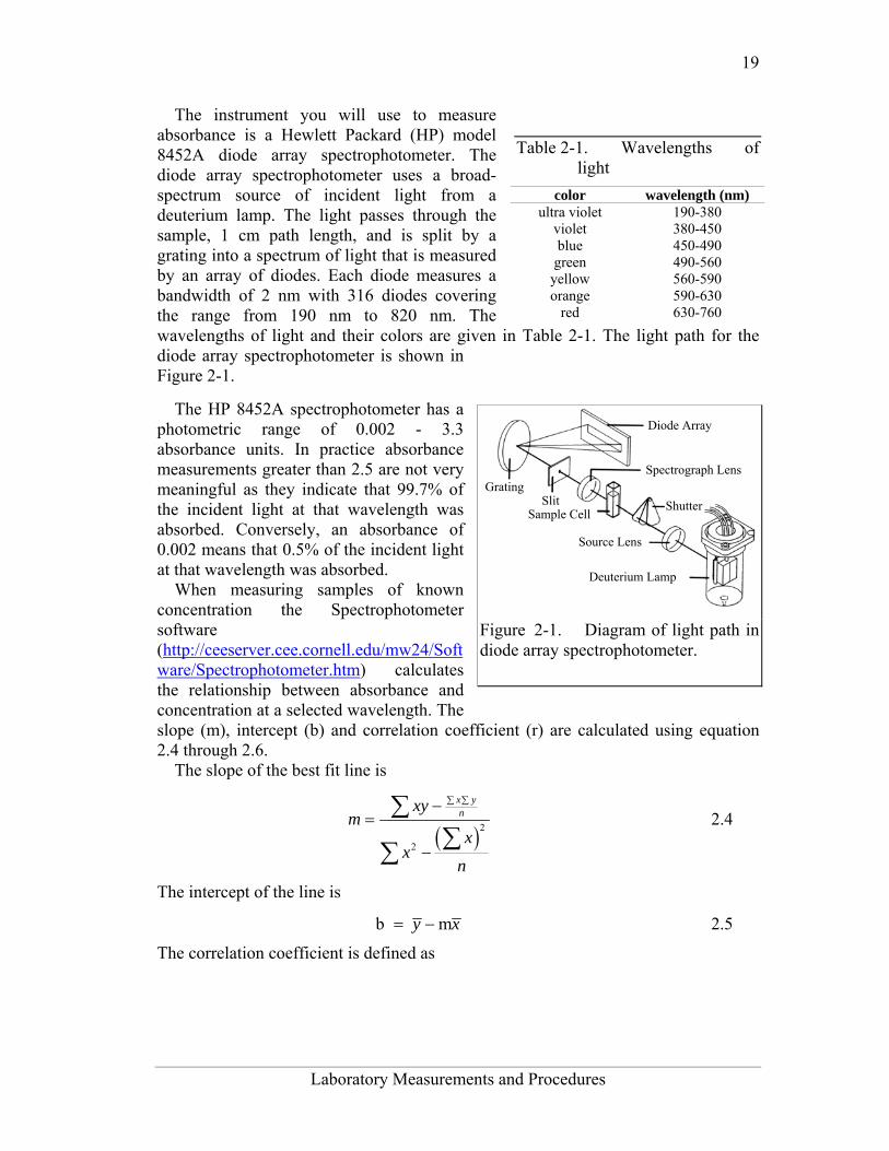
The instrument you will use to measure absorbance is a Hewlett Packard (HP) model 8452A diode array spectrophotometer. The diode array spectrophotometer uses a broad-spectrum source of incident light from a deuterium lamp. The light passes through the sample, 1 cm path length, and is split by a grating into a spectrum of light that is measured by an array of diodes. Each diode measures a bandwidth of 2 nm with 316 diodes covering the range from 190 nm to 820 nm. The wavelengths of light and their colors are given in Table 2-1. The light path for the diode array spectrophotometer is shown in Figure 2-1.

The HP 8452A spectrophotometer has a photometric range of 0.002 - 3.3 absorbance units. In practice absorbance measurements greater than 2.5 are not very meaningful as they indicate that 99.7% of the incident light at that wavelength was absorbed. Conversely, an absorbance of 0.002 means that 0.5% of the incident light at that wavelength was absorbed.

When measuring samples of known concentration the Spectrophotometer software (http://ceeserver.cee.cornell.edu/mw24/Software/Spectrophotometer.htm) calculates the relationship between absorbance and concentration at a selected wavelength. The slope (m), intercept (b) and correlation coefficient (r) are calculated using equation 2.4 through 2.6.

The slope of the best fit line is

( )2

2

x ynxy

mx

xn

∑ ∑−=

−

∑∑∑

2.4

The intercept of the line is

b my x= − 2.5

The correlation coefficient is defined as

Table 2-1. Wavelengths of light

color wavelength (nm) ultra violet 190-380

violet 380-450 blue 450-490 green 490-560

yellow 560-590 orange 590-630

red 630-760

Diode Array

Spectrograph Lens

ShutterGrating

SlitSample Cell

Source Lens

Deuterium Lamp

Figure 2-1. Diagram of light path in diode array spectrophotometer.

http://ceeserver.cee.cornell.edu/mw24/Software/Spectrophotometer.htm

20


( ) ( )2 2

2 2

x ynxy

rx y

x yn n

∑ ∑−=

⎛ ⎞⎛ ⎞⎜ ⎟⎜ ⎟− −⎜ ⎟⎜ ⎟⎝ ⎠⎝ ⎠

∑∑ ∑∑ ∑

2.6

where x is the concentration of the solute (methylene blue in this exercise), y is the absorbance, and n is the number of samples.

Experimental Objectives To gain proficiency in:

1) Calibrating and using electronic balances 2) Digital pipetting 3) Preparing a solution of known concentration 4) Preparing dilutions 5) Measuring concentrations using a UV-Vis spectrophotometer

Experimental Methods

Mass Measurements Mass can be accurately measured with an electronic analytical balance. Perhaps

because balances are so easy to use it is easy to forget that they should be calibrated on a regular basis. It is recommended that balances be calibrated once a week, after the balance has been moved, or if excessive temperature variations have occurred. In order for balances to operate correctly they also need to be level. Most balances come with a bubble level and adjustable feet. Before calibrating a balance verify that the balance is level.

The environmental laboratory is equipped with balances manufactured by Denver Instruments. To calibrate the Denver Instrument balances: 1) Zero the balance by pressing the tare button. 2) Press the MENU key until "MENU #1" is displayed. 3) Press the 1 key to select Calibrate. 4) Note the preset calibration masses that can be used for calibration on the bottom

of the display. 5) Place a calibration mass on the pan (handle the calibration mass using a cotton

glove or tissue paper). 6) The balance will automatically calibrate. A short beep will occur and the display

will read CALIBRATED for three seconds, and then return to the measurement screen.

Dry chemicals can be weighed in disposable plastic "weighing boats" or other suitable containers. It is often desirable to subtract the weight of the container in which the chemical is being weighed. The weight of the chemical can be obtained

21


either by weighing the container first and then subtracting, or by "zeroing" the balance with the container on the balance.

Temperature Measurement Use a thermistor to measure the temperature of distilled water. The thermistors are

hanging on the rack to the right of the fume hoods. The thermistor has a 4-mm diameter metallic probe. Plug the thermistor into the port labeled “temperature probe” on the signal-conditioning box (located in the cabinet next to the knee space at your workstation). The conditioned signal is connected to the laboratory data acquisition system using a red cable. Connect the red cable to one of the ports on the top row of the bench top data acquisition panel. Monitor the thermistor using pH meter software. Set the module number to 1 and the channel number to the number above the port where the red cable is connected. Verify that you are monitoring the temperature probe by holding the temperature probe in your hand and warming it up. Place the probe in a 100-mL plastic beaker full of distilled water. Wait at least 15 seconds to allow the probe to equilibrate with the solution.

Pipette Technique

1) Use Figure 2-2 to estimate the mass of 990 µL of distilled water (at the measured temperature).

2) Use a 100-1000 µL digital pipette to transfer 990 µL of distilled water to a tared weighing boat on the 100 g scale. Record the mass of the water and compare with the expected value (Figure 2-2). Repeat this step if necessary until your pipetting error is less than 2%, then measure the mass of 5 replicate 990 µL pipette samples. Calculate the mean ( x defined in equation 2.7), standard deviation (s defined in equation 2.8), and coefficient of variation, s/ x , for your measurements. The coefficient of variation (c.v.) is a good measure of the precision of your technique. For this test a c.v. < 1% should be achievable.

x

xn

= ∑ 2.7

2

s

xx

nn

2( )−

=−1

∑∑ 2.8

Note that these functions are available on most calculators and in Excel.

22


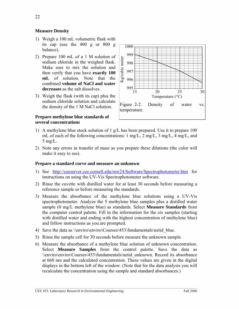
Measure Density

1) Weigh a 100 mL volumetric flask with its cap (use the 400 g or 800 g balance).

2) Prepare 100 mL of a 1 M solution of sodium chloride in the weighed flask. Make sure to mix the solution and then verify that you have exactly 100 mL of solution. Note that the combined volume of NaCl and water decreases as the salt dissolves.

3) Weigh the flask (with its cap) plus the sodium chloride solution and calculate the density of the 1 M NaCl solution.

Prepare methylene blue standards of several concentrations

1) A methylene blue stock solution of 1 g/L has been prepared. Use it to prepare 100 mL of each of the following concentrations: 1 mg/L, 2 mg/L, 3 mg/L, 4 mg/L, and 5 mg/L.

2) Note any errors in transfer of mass as you prepare these dilutions (the color will make it easy to see).

Prepare a standard curve and measure an unknown

1) See http://ceeserver.cee.cornell.edu/mw24/Software/Spectrophotometer.htm for instructions on using the UV-Vis Spectrophotometer software.

2) Rinse the cuvette with distilled water for at least 30 seconds before measuring a reference sample or before measuring the standards.

3) Measure the absorbance of the methylene blue solutions using a UV-Vis spectrophotometer. Analyze the 5 methylene blue samples plus a distilled water sample (0 mg/L methylene blue) as standards. Select Measure Standards from the computer control palette. Fill in the information for the six samples (starting with distilled water and ending with the highest concentration of methylene blue) and follow instructions as you are prompted.

4) Save the data as \\enviro\enviro\Courses\453\fundamentals\netid_blue. 5) Rinse the sample cell for 30 seconds before measure the unknown sample. 6) Measure the absorbance of a methylene blue solution of unknown concentration.

Select Measure Samples from the control palette. Save the data as \\enviro\enviro\Courses\453\fundamentals\netid_unknown. Record its absorbance at 660 nm and the calculated concentration. These values are given in the digital displays in the bottom left of the window. (Note that for the data analysis you will recalculate the concentration using the sample and standard absorbances.)

995

996

997

998

999

1000

15 20 25 30

Kg/

cubi

c m

eter

Temperature (°C) Figure 2-2. Density of water vs. temperature.

http://ceeserver.cee.cornell.edu/mw24/Software/Spectrophotometer.htm

23


7) Turn on the pump and place the sipper tube in distilled water to clean out the sample cell by selecting Run Pump from the control palette.

8) Go to one of the other computer stations in the lab to export your standards spectra to the \\enviro\enviro\Courses\453\fundamentals folder. You will need to open the spectrophotometer software and then from within the software load your standards. Then select the export function to save your standards in an Excel readable format.

Prelab Questions 1) You need 100 mL of a 1 µM solution of zinc that you will use as a standard to

calibrate an atomic adsorption spectrophotometer. Find a source of zinc ions combined either with chloride or nitrate (you can use the world wide web or any other source of information). What is the molecular formula of the compound that you found? Zinc disposal down the sanitary sewer is restricted at Cornell and the solutions you prepare may need to be disposed of as hazardous waste. As an environmental engineering you strive to minimize waste production. How would you prepare this standard using techniques readily available in the environmental laboratory so that you minimize the production of solutions that you don’t need? Note that we have pipettes that can dispense volumes between 10 µL and 1 mL and that we have 100 mL and 1 L volumetric flasks. Include enough information so that you could prepare the standard without doing any additional calculations. Consider your ability to accurately weigh small masses. Explain your procedure for any dilutions. Note that the stock solution concentration should be an easy multiple of your desired solution concentration so you don’t have to attempt to pipette a volume that the digital pipettes can’t be set for such as 13.6 µL.

2) The density of sodium chloride solutions as a function of concentration is approximately 0.6985C + 998.29 (kg/m3) (C is kg of salt/m3). What is the density of a 1 M solution of sodium chloride?

Data Analysis and Questions Submit one spreadsheet containing the data sheet, exported absorbance data, graphs

and answers to the questions. 1) Fill out the Excel data sheet located at

http://ceeserver.cee.cornell.edu/mw24/cee453/Lab_Manual/Fundamentals_data.xls. Make sure that all calculated values are entered in the spreadsheet as equations. Failure to use the spreadsheet to do the calculations will not receive full credit.

2) Create a graph of absorbance at 660 nm vs. concentration of methylene blue in Excel using the exported data file. Does absorbance at 660 nm increase linearly with concentration of methylene blue?

3) Plot ε as a function of wavelength for each of the standards on a single graph. Note that the path length is 1 cm. Make sure you include units and axis labels on your graph. If Beer’s law is obeyed what should the graph look like?

http://ceeserver.cee.cornell.edu/mw24/cee453/Lab_Manual/Fundamentals_data.xls

http://ceeserver.cee.cornell.edu/mw24/cee453/Lab_Manual/Fundamentals_data.xls

24


4) Did you use interpolation or extrapolation to get the concentration of the unknown?

5) What colors of light are most strongly absorbed by methylene blue? 6) What measurement controls the accuracy of the density measurement for the

NaCl solution? What density did you expect (see prelab 2)? Approximately what should the accuracy be?

7) Don’t forget to write a brief paragraph on conclusions and on suggestions. 8) Verify that your report and graphs meet the requirements. Check the course

website for details. (http://www.cee.cornell.edu/mw24/cee453/Lab_Reports/editing_checklist.htm and (http://www.cee.cornell.edu/mw24/cee453/Lab_Reports/default.htm)

http://ceeserver.cee.cornell.edu/mw24/cee453/Lab_Reports/editing_checklist.htm

http://www.cee.cornell.edu/mw24/cee453/Lab_Reports/default.htm

25


Data Sheet

Balance CalibrationBalance IDMass of calibration mass2nd mass used to verify calibrationMeasured mass of 2nd massTemperature MeasurementDistilled water temperaturePipette Technique (use DI-100 or Ohaus 160 balance)Density of water at that temperatureActual mass of 990 µL of pure waterMass of 990 µL of water (rep 1)Mass of 990 µL of water (rep 2)Mass of 990 µL of water (rep 3)Mass of 990 µL of water (rep 4)Mass of 990 µL of water (rep 5)Average of the 5 measurementsStandard deviation of the 5 measurementsPrecisionPercent coefficient of variation of the 5 measurementsAccuracyaverage percent error for pipettingMeasure Density (use DI-800 or Ohaus 400D or Prec. Std)Molecular weight of NaClMass of NaCl in 100 mL of a 1-M solutionMeasured mass of NaCl usedMeasured mass of empty 100 mL flaskMeasured mass of flask + 1M solutionMass of 100 mL of 1 M NaCl solutionDensity of 1 M NaCl solutionLiterature value for density of 1 M NaCl solutionpercent error for density measurmentPrepare methylene blue standards of several concentrationsVolume of 1 g/L MB diluted to 100 mL to obtain:1 mg/L MB2 mg/L MB3 mg/L MB4 mg/L MB5 mg/L MBAbsorbance of unknown at 660 nmCalculated concentration of unknown

27


Lab Prep Notes

Table 2-2. Reagent list.

Description

Supplier Catalog number

NaCl Fisher Scientific BP358-1 Methylene blue Fisher Scientific M291-25

Table 2-3. Equipment list

Description

Supplier Catalog number

Calibra 100-1095 µL

Fisher Scientific 13-707-5

Calibra 10-109.5 µL


DI 100 analytical toploader

Fisher Scientific 01-913-1A

DI-800 Toploader Fisher Scientific 01-913-1C100 mL volumetric Fisher Scientific 10-198-50

B UV-Vis

spectrophotometer Hewlett-Packard

Company 8452A

Table 2-4. Methylene Blue Stock Solution Description MW (g/M) conc. (g/L) 100 mL C16H18N3SCl 319.87 1 100.0 mg

Setup

1) Prepare stock methylene blue solution and distribute to student workstations in 15 mL vials.

2) Prepare 100 mL of unknown in concentration range of standards. Divide into two bottles (one for each spectrophotometer).

3) Verify that spectrophotometers are working (prepare a calibration curve as a test). 4) Verify that balances calibrate easily. 5) Disassemble, clean and lubricate all pipettes.

28


Acid Precipitation and Remediation of Acid Lakes

Introduction Acid precipitation has been a serious environmental problem in many areas of the

world for the last few decades. Acid precipitation results from the combustion of fossil fuels, that produces oxides of sulfur and nitrogen that react in the earth's atmosphere to form sulfuric and nitric acid. One of the most significant impacts of acid rain is the acidification of lakes and streams. In some watersheds the soil doesn’t provides ample acid neutralizing capacity to mitigate the effect of incident acid precipitation. These susceptible regions are usually high elevation lakes, with small watersheds and shallow non-calcareous soils. The underlying bedrock of acid-sensitive lakes tends to be granite or quartz. These minerals are slow to weather and therefore have little capacity to neutralize acids. The relatively short contact time between the acid precipitation and the watershed soil system exacerbates the problem. Lakes most susceptible to acidification: 1) are located downwind, sometimes hundreds of miles downwind, from major pollution sources–electricity generation, metal refining operations, heavy industry, large population centers; 2) are surrounded by hard, insoluble bedrock with thin, sandy, infertile soil; 3) have a high runoff to infiltration ratio; 4) have a low watershed to lake surface area. Isopleths of precipitation pH are depicted in Figure 3-1.

Figure 3-1. The pH of precipitation in 2000.

In acid-sensitive lakes the major parameter of concern is pH (pH = -log{H+}, where {H+} is the hydrogen ion activity, and activity is approximately equal to concentration in moles/L). In a healthy lake, ecosystem pH should be in the range of

http://nadp.sws.uiuc.edu/isopleths/

29


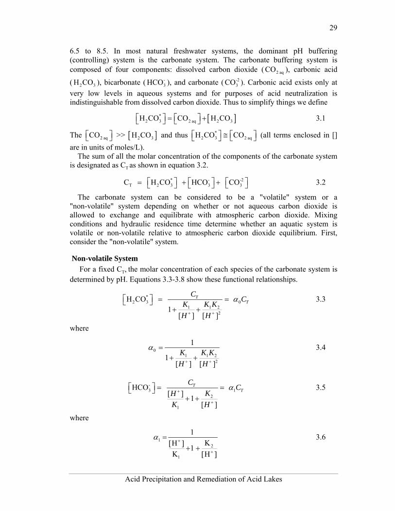
6.5 to 8.5. In most natural freshwater systems, the dominant pH buffering (controlling) system is the carbonate system. The carbonate buffering system is composed of four components: dissolved carbon dioxide ( 2 aqCO ), carbonic acid

( 2 3H CO ), bicarbonate ( -3HCO ), and carbonate ( -2

3CO ). Carbonic acid exists only at very low levels in aqueous systems and for purposes of acid neutralization is indistinguishable from dissolved carbon dioxide. Thus to simplify things we define

[ ]*2 3 2 aq 2 3H CO CO H CO⎡ ⎤ ⎡ ⎤= +⎣ ⎦⎣ ⎦ 3.1

The 2 aqCO⎡ ⎤⎣ ⎦ >> [ ]2 3H CO and thus *2 3 2 aqH CO CO⎡ ⎤ ⎡ ⎤≅ ⎣ ⎦⎣ ⎦ (all terms enclosed in []

are in units of moles/L). The sum of all the molar concentration of the components of the carbonate system

is designated as CT as shown in equation 3.2.

* - -2T 2 3 3 3C H CO HCO CO⎡ ⎤ ⎡ ⎤ ⎡ ⎤= + +⎣ ⎦ ⎣ ⎦ ⎣ ⎦ 3.2

The carbonate system can be considered to be a "volatile" system or a "non-volatile" system depending on whether or not aqueous carbon dioxide is allowed to exchange and equilibrate with atmospheric carbon dioxide. Mixing conditions and hydraulic residence time determine whether an aquatic system is volatile or non-volatile relative to atmospheric carbon dioxide equilibrium. First, consider the "non-volatile" system.

Non-volatile System For a fixed CT, the molar concentration of each species of the carbonate system is

determined by pH. Equations 3.3-3.8 show these functional relationships.

*2 3 0

1 1 22

H CO 1

[ ] [ ]

TT

C CK K KH H

α

+ +

⎡ ⎤ = =⎣ ⎦+ +

3.3

where

01 1 2

2

1

1[ ] [ ]

K K KH H

α

+ +

=+ +

3.4

-3 1

2

1

HCO [ ] 1

[ ]

TT

C CKH

K H

α+

+

⎡ ⎤ = =⎣ ⎦+ +

3.5

where

1α +2+

1

1 =

Κ[Η ]+1+

Κ [Η ]

3.6

30


-23 22

1 2 2

CO [ ] [ ] 1

TT

C CH HK K K

α+ +⎡ ⎤ = =⎣ ⎦

+ + 3.7

where

2α + 2 +

1 2 2

1 =

[Η ] [Η ]+ +1

Κ Κ Κ

3.8

K1 and K2 are the first and second dissociation constants for carbonic acid and α0, α1, and α2 are the fraction of CT in the form *

2 3H CO , -3HCO , and -2

3CO respectively. Because K1 and K2 are constants (K1 = 10-6.3

and K2 = 10-10.3), α0, α1, and α2 are only functions of pH.

A measure of the susceptibility of lakes to acidification is the acid neutralizing capacity (ANC) of the lake water. In the case of the carbonate system, the ANC is exhausted when enough acid has been added to convert the carbonate species -

3HCO , and -2

3CO to *2 3H CO . A formal definition of total acid neutralizing capacity is given

by equation 3.9.

- -2 -3 3ANC HCO 2 CO OH - H+⎡ ⎤ ⎡ ⎤ ⎡ ⎤ ⎡ ⎤= + +⎣ ⎦ ⎣ ⎦ ⎣ ⎦ ⎣ ⎦ 3.9

ANC has units of equivalents per liter. The hydroxide ion concentration can be obtained from the hydrogen ion concentration and the dissociation constant for water Kw.

-OH H

wK+

⎡ ⎤ =⎣ ⎦ ⎡ ⎤⎣ ⎦ 3.10

Substituting equations 3.5, 3.7, and 3.10 into equation 3.9, we obtain

( ) HH

wT

KANC C α α +

1 2 +⎡ ⎤= + 2 + − ⎣ ⎦⎡ ⎤⎣ ⎦

3.11

For the carbonate system, ANC is usually referred to as alkalinity.1

Volatile Systems: Now consider the case where aqueous 2 aqCO is volatile and in equilibrium with

atmospheric carbon dioxide. Henry's Law can be used to describe the equilibrium relationship between atmospheric and dissolved carbon dioxide.

22 aq CO HCO P K⎡ ⎤ =⎣ ⎦ 3.12

1 Alkalinity can be expressed as equivalents/L or as mg/L (ppm) of CaCO3. 50,000

mg/L CaCO3 = 1 equivalent/L.

31


where KH is Henry's constant for CO2 in moles/L-atm and PCO2 is partial pressure of

CO2 in the atmosphere (KH = 10-1.5 and PCO2 = 10-3.5). Because 2 aqCO⎡ ⎤⎣ ⎦ is

approximately equal to *2 3H CO⎡ ⎤⎣ ⎦ and from equations 3.1 and 3.3

2 0CO H TP K Cα= 3.13

2TC CO HP K

a0

= 3.14

Equation 3.14 gives the equilibrium concentration of carbonate species as a function of pH and the partial pressure of carbon dioxide.

The acid neutralizing capacity expression for a volatile system can be obtained by combining equations 3.14 and 3.11.

2 HH

CO H wP K K

ANCa

α α +1 2 +

0

⎡ ⎤= ( + 2 ) + − ⎣ ⎦⎡ ⎤⎣ ⎦ 3.15

In both non-volatile and volatile systems, equilibrium pH is controlled by system

ANC. Addition or depletion of any ANC component in equation 3.11 or 3.15 will result in a pH change. Natural bodies of water are most likely to approach equilibrium with the atmosphere (volatile system) if the hydraulic residence time is long and the body of water is shallow.

Lake ANC is a direct reflection of the mineral composition of the watershed. Lake watersheds with hard, insoluble minerals yield lakes with low ANC. Typically watersheds with soluble, calcareous minerals yield lakes with high ANC. ANC of freshwater lakes is generally composed of bicarbonate, carbonate, and sometimes organic matter ( -

orgA ). Organic matter derives from decaying plant matter in the watershed. When organic matter is significant, the ANC becomes (from equations 3.11 and 3.15):

-org H A

Hw

TK

ANC C α α +1 2 +

⎡ ⎤ ⎡ ⎤= ( + 2 ) + − +⎣ ⎦ ⎣ ⎦⎡ ⎤⎣ ⎦ 3.16

2 -orgH A

HCO H w

P K KANC

aα α +

1 2 +0

⎡ ⎤ ⎡ ⎤= ( + 2 ) + − +⎣ ⎦ ⎣ ⎦⎡ ⎤⎣ ⎦ 3.17

where equation 3.16 is for a non-volatile system and equation 3.17 is for a volatile system.

During chemical neutralization of acid, the components of ANC associate with added acid to form protonated molecules. For example:

- *3 2 3H HCO H CO+⎡ ⎤ ⎡ ⎤ ⎡ ⎤+ → ⎣ ⎦ ⎣ ⎦ ⎣ ⎦ 3.18

or

32


-org orgH A HA+⎡ ⎤ ⎡ ⎤ ⎡ ⎤+ → ⎣ ⎦⎣ ⎦ ⎣ ⎦ 3.19

In essence, the ANC of a system is a result of the reaction of acid inputs to form associated acids from basic anions that were dissolved in the lake water. The ANC (equation 3.9) is consumed as the basic anions are converted to associated acids. This conversion is near completion at low pH (approximately pH 4.5 for the bicarbonate and carbonate components of ANC). Neutralizing capacity to another (probably higher) pH may be more useful for natural aquatic systems. Determination of ANC to a particular pH is fundamentally easy — simply add and measure the amount of acid required to lower the sample pH from its initial value to the pH of interest. Techniques to measure ANC are described under the procedures section of this lab.

Neutralization of acid precipitation can occur in the watershed or directly in the lake. How much neutralization occurs in the watershed versus the lake is a function of the watershed to lake surface area. Generally, watershed neutralization is dominant. Recently engineered remediation of acid lakes has been accomplished by adding bases such as limestone, lime, or sodium bicarbonate to the watershed or directly to the lakes.

Reactor theory applied to Acid Lake Remediation In this experiment sodium bicarbonate will be added to a lake to mitigate the

deleterious effect of acid rain. Usually sodium bicarbonate is added in batch doses (as opposed to metering in). The quantity of sodium bicarbonate added depends on how long a treatment is desired, the acceptable pH range and the quantity and pH of the incident rainfall. For purposes of this experiment, a 15-minute design period will be used. That is, we would like to add enough sodium bicarbonate to keep the lake at or above its original pH and alkalinity for a period of 15 minutes (i.e. for one hydraulic residence time).

By dealing with ANC instead of pH as a design parameter, we avoid the issue of whether the system is at equilibrium with atmospheric carbon dioxide. Keep in mind that eventually the lake will come to equilibrium with the atmosphere. In practice, neutralizing agent dosages may have to be adjusted to take into account non-equilibrium conditions.

We must add enough sodium bicarbonate to equal the negative ANC from the acid precipitation input plus the amount of ANC lost by outflow from the lake during the 15-minute design period. Initially (following the dosing of sodium bicarbonate) the pH and ANC will rise, but over the course of 15 minutes, both parameters will drop. Calculation of required sodium bicarbonate dosage requires performing a mass balance on ANC around the lake. This mass balance will assume a completely mixed lake and conservation of ANC. Chemical equilibrium can also be assumed so that the sodium bicarbonate is assumed to react immediately with the incoming acid precipitation. Mass balance on the reactor yields:

( )in outd(ANC)Q ANC - ANC V

dt= 3.20

where:

33


ANCout = ANC in lake outflow at any time t (for a completely mixed lake the effluent ANC is the same as the ANC in the lake)

ANCin = ANC of acid rain input V = volume of reactor Q = acid rain input flow rate.

If the initial ANC in the lake is designated as ANC0, then the solution to the mass balance differential equation is:

( ) 01 -t/ -t/ out inANC ANC - ANCe eθ θ= ⋅ + ⋅ 3.21

where: θ = V/Q We want to find ANC0 such that ANCout = 50 µeq/L when t is equal to θ. Solving

for ANC0 we get

( )0 out inANC ANC - ANC 1 -t/ t/ - e eθ θ⎡ ⎤= ⋅⎣ ⎦ 3.22

The ANC of the acid rain (ANCin) can be estimated from its pH. Below pH 6.3 most of the carbonates will be in the form *

2 3H CO and thus for pH below about 4.3 equation 3.9 simplifies to

ANC H+⎡ ⎤≅ − ⎣ ⎦ 3.23

An influent pH of 3.0 implies the ANCin = - H+⎡ ⎤⎣ ⎦ = -0.001 Substituting into equation 3.22:

( )1 10ANC 0.000050 0.001 1 - - e e⎡ ⎤= + ⋅⎣ ⎦ = 1.854 meq/L 3.24

The quantity of sodium bicarbonate required can be calculated from:

[NaHCO3]0 =ANC0 3.25

where [NaHCO3]0 = moles of sodium bicarbonate required per liter of lake water

3 33

3

1.854 mmole NaHCO 84 mg NaHCO× × 4 Liters = 623 mg NaHCOliter mmole NaHCO

3.26

Experimental Objectives Remediation of acid lakes involves addition of ANC so that the pH is raised to an

acceptable level and maintained at or above this level for some design period. In this experiment sodium bicarbonate (NaHCO3) will be used as the ANC supplement. Since ANC addition usually occurs as a batch addition, the design pH is initially exceeded. ANC dosage is selected so that at the end of the design period pH is at the acceptable level. Care must be taken to avoid excessive initial pH — high pH can be as deleterious as low pH.

34


The most common remediation procedure is to apply the neutralizing agent directly to the lake surface, instead of on the watershed. We will follow that practice in this lab experiment. Sodium bicarbonate will be added directly to the surface of the lake that has an initial ANC of 0 µeq/L and is receiving acid rain with a pH of 3. After the sodium bicarbonate is applied, the lake pH and ANC will be monitored for approximately one hour.

Experimental Apparatus The experimental apparatus consists of an acid rain storage reservoir, peristaltic

pump, and lake (Figure 3-2). The pH of the lake will be monitored using a pH probe connected to a signal-conditioning box that is connected to the laboratory data acquisition system.

Experimental Procedures The following directions are written

assuming the use of the pH software and manual control of the peristaltic pump. It would also be possible to use the Process Control software to automate the experiment..

Warning: pH signal conditioning boxes must not be connected to the data acquisition system unless they have a pH probe or a “cap” connected. Otherwise they will cause the data acquisition system to give erroneous readings on all channels. 1) Calibrate the pH probe by rinsing the probe with distilled water, immersing the

probe in one of the pH buffer solutions, stirring the solution gentle, wait for the pH to stabilize and then press the “add buffer” button on the pH software. Repeat for each of the 3 pH buffers

2) Verify that the system is plumbed so that the “acid rain” is pumped directly into the lake.

3) Take a 50-mL sample from the acid rain container. Collect the sample in a 125-mL bottle.

4) Preset pump to give desired flow rate of 267 mL/min (4 L/15 minutes). 5) Fill lake with distilled water and verify that the outflow is set so the lake volume

is approximately 4 L. 6) Set stirrer speed to 8. 7) Add 1 mL of bromocresol green indicator solution to the lake. 8) Weigh out 623 mg (not grams!) NaHCO3. 9) Add NaHCO3 to the lake.

10) After the lake is well stirred take a 100 mL sample from the lake. 11) Place the pH probe in the lake.

Feed solution

Peristaltic pump

Lake

Lake effluent

Figure 3-2. Schematic drawing of the experimental setup.

35


12) Label sample bottles (see step 14). 13) Set the data interval to 1 second.

14) Begin logging data to file by clicking on the button. Create a new file in \\enviro\enviro\courses\453\acid rain with your netids in the name.

15) Prepare to write a comment in the file to mark the time when the pump starts by

clicking on the button. Type in a comment and then wait. 16) At time equal zero start the peristaltic pump and click on the enter button in the

comment dialog box. 17) Take 100-mL grab samples from the lake effluent at 5, 10, 15, and 20 minutes.

The sample volumes do not need to be measured. Collect the samples in 125-mL bottles.

18) Measure the flow rate. 19) After the 20-minute sample turn off the pump and stop sampling pH. 20) Measure the lake volume. 21) Repeat the experiment and change one of the following parameters: stirring,

initial ANC, ANC source (use CaCO3 instead of Na2CO3)

Analytical Procedures pH. pH (-log{H+}) is usually measured electrometrically with a pH meter. The pH

meter is a null-point potentiometer that measures the potential difference between an indicator electrode and a reference electrode. The two electrodes commonly used for pH measurement are the glass electrode and a reference electrode. The glass electrode is an indicator electrode that develops a potential across a glass membrane as a function of the activity ,~ molarity, of H+. Combination pH electrodes, in which the H+-sensitive and reference electrodes are combined within a single electrode body will be used in this lab. The reference electrode portion of a combination pH electrode is a [Ag/AgCl/4M KCl] reference. The response (output voltage) of the electrode follows a "Nernstian" behavior with respect to H+ ion activity.

0

0 lnHRTE E

nF H

+

+

⎛ ⎞⎡ ⎤⎣ ⎦⎜ ⎟= + ⎜ ⎟⎡ ⎤⎜ ⎟⎣ ⎦⎝ ⎠

3.27

where R is the universal gas constant, T is temperature in Kelvin, n is the charge of the hydrogen ion, and F is the Faraday constant. E0 is the calibration potential (Volts), and E is the potential (Volts) measured by the pH meter between glass and reference electrode. The slope of the response curve is dependent on the temperature of the sample and this effect is normally accounted for with simultaneous temperature measurements.

The electrical potential that is developed between the glass electrode and the reference electrode needs to be correlated with the actual pH of the sample. The pH meter is calibrated with a series of buffer solutions whose pH values encompass the

36


range of intended use. The pH meter is used to adjust the response of the electrode system to ensure a Nernstian response is achieved over the range of the calibration standards.

To measure pH the electrode(s) are submersed in at least 50 mL of a sample. Samples are generally stirred during pH reading to establish homogeneity, to prevent local accumulation of reference electrode filling solution at the interface near the electrode, and to ensure the diffusive boundary layer thickness at the electrode surface is uniform and small.

ANC. The most common method to determine ANC for aqueous samples is titration with a strong acid to an endpoint pH. A pH meter is usually used to determine the endpoint or "equivalence point" of an ANC titration. Determination of the endpoint pH is difficult because it is dependent on the magnitude the sample ANC. Theoretically this endpoint pH should be the pH where all of the ANC of the system is consumed, but since the ANC is not known a-priori, a true endpoint cannot be predetermined. However, if most of the ANC is composed of carbonate and bicarbonate this endpoint is approximately pH = 4.5 for a wide range of ANC values.

A 50 to 100-mL sample is usually titrated while slowly stirred by a magnetic stirrer. pH electrodes are ordinarily used to record pH as a function of the volume of strong acid titrant added. The volume of strong acid required to reach the ANC endpoint (pH 4.5) is called the "equivalent volume" and is used in the following equation to compute ANC.

(equivalent vol.)(normality of titrant)ANC =(vol. of sample)

3.28

A more accurate technique to measure ANC is the Gran plot analysis. This is the subject of a subsequent experiment. All ANC samples should be labeled and stored for subsequent Gran analysis.

Prelab Questions 1) How many grams of NaHCO3 would be required to keep the ANC levels in a lake

above 50 µeq/L for 3 hydraulic residence times given an influent pH of 3.0 and a lake volume of 4 L, if the current lake ANC is 0 µeq/L?

Data Analysis K1 = 10-6.3, K2 = 10-10.3, KH = 10-1.5 mol/atm L, PCO2

= 10-3.5 atm, and Kw = 10-14.

1) Plot measured pH of the lake versus hydraulic residence time (t/θ). 2) Given that ANC is a conservative parameter and that the lake is essentially in a

completely mixed flow regime equation 3.21 applies. Graph the predicted ANC based on the completely mixed flow reactor equation with the plot labeled (in the legend) as “conservative ANC.”

3) Derive an equation for CT (the concentration of carbonate species) as a function of time based on the input of NaHCO3 and its dilution in the completely mixed lake assuming that no carbonate species are lost or gained to the atmosphere (the

37


equation will be the same form as equation 3.21). Plot this conservative CT versus hydraulic residence time (t/θ).

4) Derive an equation for CT as a function of ANC and pH based on equation 3.11. Use the CMFR model to obtain ANC as a function of time. Plot this measured CT versus hydraulic residence time (t/θ) on the same graph as above.

5) Plot the equilibrium concentration of CT (a function of pH) versus hydraulic residence time (t/θ) on the same graph as above.

6) Compare the plots and determine whether the lake is best modeled as a volatile or non-volatile system. What changes could be made to the lake to bring the lake into equilibrium with atmospheric CO2?

7) Analyze the data from the 2nd experiment and graph the data appropriately. What did you learn from the 2nd experiment?

Questions 1) What do you think would happen if enough NaHCO3 were added to the lake to

maintain an ANC greater than 50 µeq/L for 3 residence times with the stirrer turned off? How much NaHCO3 would need to be added?

2) What are some of the complicating factors you might find in attempting to remediate a lake using CaCO3? Below is a list of issues to consider. • extent of mixing • solubility of CaCO3 (find the solubility and compare with NaHCO3) • density of CaCO3 slurry (find the density of CaCO3)

References Driscoll, C.T., Jr. and Bisogni, J.J., Jr., "Weak Acid/Base Systems in Dilute Acidified

Lakes and Streams of the Adirondack Region of New York State," in Modeling of Total Acid Precipitation Impacts J.L. Schnoor (ed.), Butterworth, Stoneham, MA., 53-72 (1983).

Driscoll, C.T., Baker, J.P., Bisogni, J.J., And Schofield, C.L., "Aluminum Speciation and Equilibria in Dilute Surface Waters of the Adirondack Region of New York State," in Geological Aspects of Acid Deposition O.P. Bricker (ed.), Butterworth, Stoneham, MA., 55-75 (1984).

Barnard. T.E., And Bisogni, J.J., Jr., "Errors in Gran Function Analysis of Titration Data for Dilute Acidified Water," Water Research, 19, No. 3 393-399 (1985).

Bisogni, J.J., Jr. and Barnard, T.E., "Numerical Technique to Correct for Weak Acid Errors in Gran Function Analysis of Titration Data," Water Research, 21, No. 10, 1207-1216 (1987).

Bisogni, J.J., Jr., "Fate of Added Alkalinity During Neutralization of an Acid Lake," Journal Environmental Engineering, ASCE, 114, No. 5, 1219-1224 (1988).

Bisogni, J.J., Jr., and Kishbaugh, S.A., "Alkalinity Destruction by Sediment Organic Matter Dissolution During Neutralization of Acidified Lakes," Water, Air and Soil Pollution, 39, 85-95 (1988).

38


Bisogni, J.J., Jr. and Arroyo, S.L., "The Effect of Carbon Dioxide Equilibrium on pH in Dilute Lakes," Water Research, 25, No. 2, 185-190 (1991).

Olem, H. Liming Acidic Surface Waters. Lewis Publishers, Chelsea, MI. (1991). Stumm, W. and Morgan, J.J., Aquatic Chemistry, John Wiley & Sons, Inc. NY, NY

1981.

39


Lab Prep Notes

Bromocresol Green Indicating Solution

Prepare solution of 400 mg Bromocresol green/100 mL ethanol. Add 0.2 mL of indicator solution per liter of acid rain or lake.

Acid rain Acid rain is at pH 3.0. Prepare

from distilled water. Add 1 meq H2SO4/L ([H+] at pH 3.0) to obtain a pH of 3.0. To acidify 20 liters of distilled water using 5 N H2SO4:

2 4

2 42 4

1 meq H SO 1 1N L20 L = 4 mL of 5 N H SOL 5 N H SO 1000 meq

⋅ ⋅ ⋅

Add 4 mL of bromocresol green

indicating solution to 20 L of acid rain solution.

Flow Rate The residence time of the lake

should be 15 minutes. The lake volume is 4 L. thus the flow rate is 267 mL/min. Use # 18 PharMed tubing.

Setup

1) Prepare 20-L acid rain for each group.

2) Prepare bromocresol green solution if necessary.

3) Attach one Easy-Load pump head to the pump drives and plumb with #18 tubing. 4) Plumb Jerrican to pump to lake using quick connectors (see Figure 3-2). 5) Verify that pH probes are operational, stable, and can be calibrated. 6) Verify that buffers (pH = 4, 7, 10) are distributed to each student group. 7) Provide a mount for the pH probe in the lake. 8) Provide equipment for aeration so students can add this if they want.

Table 3-1. Reagents

Description Supplier Catalog number

HCL 5.0 N Fisher Scientific LC15360-2 H2SO4 5N Fisher Scientific LC25840-2

CaCO3 Fisher Scientific C63-3 Na2CO3 Fisher Scientific S263-500

Buffer-Pac Fisher Scientific SB105 NaHCO3 Fisher Scientific S233-500

Bromocresol Green

Fisher Scientific B383-5

ethanol Fisher Scientific A962P-4


Description Supplier Catalog number

magnetic stirrer Fisher Scientific 11-500-7S floating stir bar Fisher Scientific 14-511-99A Accumet™ 50

pH meter Fisher Scientific 13-635-50

100-1095 µL pipette


10-109.5 µL pipette


pH electrode Fisher Scientific 13-620-108 6 L container

(lake) Fisher Scientific 03-484-22

Easy load pump head

Cole Parmer H-07518-00

digital pump drive

Cole Parmer H-07523-30_

PharMed tubing size 18


20 liter HDPE Jerrican

Fisher Scientific 02-961-50C

40


Measurement of Acid Neutralizing Capacity

Introduction Acid neutralizing capacity (ANC) is a measure of the ability of water to neutralize

acid inputs. Lakes with high ANC (such as Cayuga Lake) can maintain a neutral pH even with some acid rain input whereas lakes with an ANC less than the acid input will not maintain a neutral pH. In the Adirondack region of New York State, lakes typically receive large inputs of acids during the spring thaw when the accumulated winter snow melts and runs off into the lakes. The ANC of Adirondack lakes is not always sufficient to neutralize these inputs.

Theory The ANC for a typical carbonate-containing sample is defined as:

- -2 -3 3ANC [HCO ] 2[CO ] [OH ] - [H ]+= + + 4.1

This equation can be derived from a charge balance if ANC is considered to be the cation contributed by a strong base titrant and if other ions present do not contribute significantly.

Determination of ANC or Alkalinity involves determination of an equivalence point. The equivalence point is defined as the point in the titration where titrant volume that has been added equals the "equivalent" volume (Ve). The equivalent volume is defined as:

·

= s se

t

V NV

N 4.2

where: Ns = normality (in this case Alkalinity or ANC) of sample, equivalents/L Vs = volume of sample, liters Nt = normality of titrant, equivalents/L.

The titration procedure involves incrementally adding known volumes of

standardized normality strong acid (or base) to a known volume of unknown normality base (or acid). When enough acid (or base) has been added to equal the amount of base (or acid) in the unknown solution we are at the "equivalence" point. (Note: the point at which we add exactly an equivalent or stoichiometric amount of titrant is the equivalence point. Experimentally, the point at which we estimate to be the equivalence point is called the titration endpoint).

There are several methods for determining Ve (or the equivalence point pH) from titration data (titrant volume versus pH). The shape of the titration curve (Vt versus pH) can reveal Ve. It can be shown that one inflection point occurs at t eV V= . In the case of monoprotic acids, there is only one inflection in the pH range of interest. Therefore, an effective method to find the equivalence volume is to plot the titration curve and find the inflection point. Alternately, plot the first derivative of the titration plot and look for a maximum.

41


Gran Plot Another method to find the ANC of an unknown solution is the Gran plot

technique. When an ANC determination is being made, titration with a strong acid is used to "cancel" the initial ANC so that at the equivalence point the sample ANC is zero. The Gran plot technique is based on the fact that further titration will result in an increase in the number of moles of H+ equal to the number of moles of H+ added. Thus after the equivalence point has been reach the number of moles of H+ added equals the number of moles of H+ in solution.

( ) ( )t t e s tN V V V V H +⎡ ⎤− = + ⎣ ⎦ 4.3

Solving for the hydrogen ion concentration:

( )

( )t t e

s t

N V VH

V V+ −

⎡ ⎤ =⎣ ⎦ + 4.4

Equation 4.4 can be solved directly for the equivalent volume.

( )s t

e tt

H V VV V

N

+⎡ ⎤ +⎣ ⎦= − 4.5

Equation 4.5 is valid if enough titrant has been added to neutralize the ANC. A better measure of the equivalent volume can be obtained by rearranging equation 4.4 so that linear regression on multiple titrant volume - pH data pairs can be used.

( )s t t t t e

s s s

V V N V N VH

V V V++

⎡ ⎤ = −⎣ ⎦ 4.6

We define F1 (First Gran function) as:

1F [H ]s t

s

V VV

++= 4.7

If F1 is plotted as a function of Vt the result is a straight line with slope =

t

s

NV

and abscissa intercept of Ve

(Figure 4-1). The ANC is readily obtained

given the equivalent volume. At the equivalence pt:

s e tV ANC V N= 4.8

Equation 4.8 can be rearranged to obtain ANC as a function of the equivalent volume.

y = 9.57E-04x - 4.62E-03R2 = 9.99E-01

00.00010.00020.00030.00040.00050.00060.00070.00080.0009

0 1 2 3 4 5 6

Volume of Titrant (mL)

Gran Function

Gran Function Linear Region

Figure 4-1. Gran plot from titration of a weak base with 0.05 N acid. Ct = 0.001 moles of carbonate and sample volume is 48 mL. The equivalent volume is 4.8 mL. From equation 4.9 the ANC is 5 meq/L.

42


ANC e t

s

V NV

= 4.9

pH Measurements The pH can be measured either as activity ({H+} as measured approximately by pH

meter) or molar concentration ([H+]). The choice only affects the slope of F1 since [H+] = {H+}/γ.

1{ }F [H ] s t s t t e

ts s s

V V V V V VHV V Vγ

+++ + −

= = = Ν 4.10

where γ is the activity correction factor and the slope is Nt/V0. If H+ concentration is

used then

1 tF {H } Ns t t e

s s

V V V VV V

γ++ −= = 4.11

where the slope is t

sVγ ⋅ Ν

.

(This analysis assumes that the activity correction factor doesn't change appreciably during the titration).

There are many other Gran functions that can be derived. For example, one can be derived for Acidity or the concentration of a single weak or strong acid or base.

To facilitate data generation and subsequent Gran plot construction and analysis pH versus titrant volume can be read directly into a computer, that can be programmed to analyze the data using the Gran, plot theory. The program generates the Gran function for all data and then systematically eliminates data until the Gran function (plot) is as linear as possible. The line is then extrapolated to the abscissa to find the equivalent volume.

ANC Determination for Samples with pH < 4 After the equivalence point has been reached (adding more acid than ANC = 0) the

only significant terms in equation 4.1 are H+⎡ ⎤⎣ ⎦ and ANC.

- -2 -3 3H HCO 2 CO OH +⎡ ⎤ ⎡ ⎤ ⎡ ⎤ ⎡ ⎤>> + +⎣ ⎦ ⎣ ⎦ ⎣ ⎦ ⎣ ⎦ 4.12

When the pH is 2 pH units or more below the pKs of the bases in the system the only species contributing significantly to ANC is the hydrogen ion (equation4.12) and thus the ANC is simply

ANC - [H ]+= 4.13

For a sample containing only carbonates, if the pH is below 4 the ANC is approximately equal to -[H+] and no titration is necessary.

43


Titration Techniques Operationally, the first few titrant volumes can be relatively large increments since

the important data lies at pH values less than that of the equivalence point (approximately pH = 4.5 for an Alkalinity titration). As the pH is lowered by addition of acid the ionic strength of the solution increases and the activity of the hydrogen ion deviates from the hydrogen ion concentration This effect is significant below pH 3 and thus the effective linear range is generally between pH 4.5 and pH 3.0. The maximum incremental titrant volume (∆Va) that will yield n points in this linear region is obtained as follows. If Vs » Vt then equation 4.3 reduces to

t( )

N [H ]t e

s

V VV

+−≅ 4.14

Let [H+]e be the concentration of hydrogen ions at the equivalence point and [H+]f be the final concentration of hydrogen ions at the end of the titration.

t e f

( ) ( )N [H ] - [H ]e e f e

s

V V V VV

+ +− − −= 4.15

Thus the volume of acid added to go from [H+]e to [H+]f is

( )

f e

[ ] [ ]V - V s f e

t

V H H

N

+ +−= 4.16

To obtain n data points between [H+]e - [H+]f requires the incremental titrant volume

(∆Vt) be 1/n times the volume of acid added between the equivalence point and the final titrant volume. Thus by substituting n∆Vt, and typical hydrogen ion concentrations of [H+]e = 10-4.5 and [H+]f = 10-3.0 into equation 4.16 the maximum incremental titrant volume is obtained.

t(0.001 0.00003) 0.001

V

s s

t t

V Vn N n N

−∆ ≅ ≅ 4.17

Procedure

Calibrate the pH Probe Calibrate the pH probe using 3 standards (pH = 4, 7, and 10).

Determine ANC of a Known Standard Do the following procedure twice. The first time titrate as fast as possible and learn

how the software works. Then repeat the procedure with the goal of making an accurate ANC measurement and creating an accurate titration curve by using 0.25 mL titrant increments throughout the entire titration. Remember that the biggest source of error for this lab will likely be poor pipette techniques.

44


1) Weigh a 100 mL plastic beaker. 2) Add approximately 50 mL of a 2.5 mM solution of Na2CO3 to the beaker.

3) Weigh the beaker again to determine the exact volume of Na2CO3 solution.

4) Place the beaker on the magnetic stirrer, add a stir bar and stir slowly. 5) Place both the pH electrode and the temperature probe in the Na2CO3 solution.

6) Analyze the sample using Gran plot analysis as detailed at http://ceeserver.cee.cornell.edu/mw24/Software/ph_meter.htm) Add 0.05 N HCl (the titrant) using a digital pipette in increments of 0.25 mL.

7) Save the Gran data to \\Enviro\enviro\Courses\453\acid\netid_gran by selecting

. The data will be saved in a file (tab delimited format) that can be opened by any spreadsheet program. You will use this data to plot a titration curve and to verify that the Gran technique accurately measures the ANC of a sample.

8) Record the ANC and the equivalent volume. If the error is greater than 2% then check your pipette technique using a balance and then repeat the titration.

Determine ANC of Acid Rain Samples Determine ANC for all samples collected from the previous week's lab. Use the

same technique as outlined above (Determine ANC of known standard) except substitute the samples collected last week and use titrant increment of 0.1 mL in the linear region. For samples that have a high ANC you can reduce the analysis time by adding titrant in larger volumes initially until the pH approaches 5. If the initial pH is less than 4.5 no titration is necessary and equation 4.13 can be used to calculate the ANC.

Record the initial pH (prior to adding any titrant) and initial sample volume. After the Gran plot analysis record the alkalinity (ANC) and equivalent volume for each sample. There is no need to save the data to disk.

Prelab Questions 1) Compare the ability of Cayuga lake and Wolf pond (an Adirondack lake) to

withstand an acid rain runoff event (from snow melt) that results in 20% of the original lake water being replaced by acid rain. The acid rain has a pH of 3.5 and is in equilibrium with the atmosphere. The ANC of Cayuga lake is 1.6 meq/L and the ANC of Wolf Pond is 70 µeq/L. Assume that carbonate species are the primary component of ANC in both lakes, and that they are in equilibrium with the atmosphere. What is the pH of both bodies of water after the acid rain input? Remember that ANC is the conservative parameter (not pH!).

2) What is the ANC of a water sample containing only carbonates and a strong acid that is at pH 3.2?

3) Why is [H+] not a conserved species?

http://www.cee.cornell.edu/mws/Software/Compumet.htm

45


Questions 1) Plot the titration curve of 2.5 mM Na2CO3 with 0.05 N HCl (plot pH as a function

of titrant volume). Label the equivalent volume of titrant. Label the 2 regions of the graph where pH changes slowly with the dominant reaction that is occurring. Type the chemical reactions in textboxes and place them on the graph in the pH regions where each reaction is occurring.) Note that in a third region of slow pH change no significant reactions are occurring (added hydrogen ions contribute directly to change in pH).

2) Prepare a Gran plot using the data from the titration curve of the 2.5 mM Na2CO3. Use linear regression on the linear region or simply draw a straight line through the linear region of the curve to identify the equivalent volume. Compare your calculation of Ve with that calculated by the pH meter computer program.

3) Compare the measured ANC with the theoretical value for the 2.5 mM Na2CO3 solution. Note that ANC can be defined as the excess of positive charges over the anions of strong acids. Thus for the 2.5 mM Na2CO3 solution the ANC is 5 meq/L since there are 5 meq/L of Na+

and no anions of strong acids. 4) Plot the measured ANC of the lake on the same graph as was used to plot the

conservative, volatile, and nonvolatile ANC models (see questions 2 to 5 on page 36). Did the measured ANC values agree with the conservative ANC model?

Writing a High Performance Report Writing will be an important part of your professional career. Your objectives in

writing may be to present recommendations or explain options to a client. In that case you will be telling the client a story (or stories) that you create to explain the facts (or data) from your investigation. You will want to explain how the different pieces of your investigation fit together and how they lead to the recommendation that you propose.

For the laboratory report that you will be writing in the next few days imagine the following scenario. Under pressure from energy companies, the EPA has decided to increase allowances of sulfur dioxide and nitrous oxide from coal fired generating plants. Your consulting firm has won a contract (with funding from EPA and ARM & HAMMER) to assess the feasibility of maintaining the pH of Adirondack lakes in the range of 6.5 to 8.2 given the increased input of acid. Your specialty in the consulting firm is aquatic chemistry and your task has been to develop a model that describes the response of acidic lakes to remediation with the goal of providing guidance on how much sodium bicarbonate to add to the lakes and how frequently to add it.

As you write your report you can weave what you have learned into your recommendations. This report should incorporate what you learned from both the acid lake lab and the Gran analysis. If you wish you could pretend that the results that you obtained were for a small Adirondack pond. In weaving your story you might consider answering the following questions. 1) Why is it important to know the extent of carbon dioxide exchange with the

atmosphere? 2) Why have you chosen to analyze the lake using the techniques that you used?

46


3) How do the dissociation constants for the carbonate system affect the ability to maintain the lake pH in the desired range?

4) What is your recommendation for how to add the sodium bicarbonate to the lakes and what complications do you anticipate?

5) How would you determine whether other Adirondack lakes are exchanging significant quantities of carbon dioxide with the atmosphere?

6) What monitoring program would you propose to access the impact of your remediation strategy?

7) What services might you offer to your client as ways that you could provide further guidance while they implement this remediation project? (You would like them to offer you a continuing contract…)

References Sawyer, C.N., P.L. McCarty and G.F. Parkin Chemistry for Environmental

Engineering, 4th ed., McGraw-Hill (1994). Pankow, J.F. Aquatic Chemistry Concepts, Lewis Publishers (1991). Morel, F.M.M. and J.G. Hering Principles and Applications of Aquatic Chemistry

Wiley-Interscience (1993). Stumm, W. and J.J. Morgan Aquatic Chemistry 2nd ed. Wiley Interscience (1981).

47


Lab Prep Notes

Table 4-1. Reagent list. Description Supplier Catalog

number HCl 5.0 N Fisher Scientific LC15360-2 Buffer-Pac Fisher Scientific SB105

Na2CO3 Fisher Scientific BP357-1

Table 4-2. Equipment list Description Supplier Catalog

number Accumet™ 50

pH meter Fisher Scientific 13-635-50

pH electrode Fisher Scientific 13-620-108 7x7 stirrer Fisher Scientific 11-500-7S

stirbar 1/2" long Fisher Scientific 14-511-62 100 mL Fisher

beaker Fisher Scientific 02-593-50B

Setup

1) Prepare 1 L of the known standard (2.5 mM solution of Na2CO3). The MW is 105.99 g/mole. 2.5mM

L· 105.99mg

mM= 265 mg Na2CO3/L

2) Prepare 1 L of the titrant (0.05 N HCl from 5.0 N HCl). Dilute 10 mL of 5.0 N HCl to 1 L. Distribute 100 mL titrant to each student group.

3) Verify that the pH probes are operational, stable, and can be calibrated. 4) Verify that buffers (pH = 4, 7, 10) are distributed to each student group

48


Reactor Characteristics

Introduction Chemical, biological and physical processes in nature and in engineered systems

usually take place in what we call "reactors." Reactors are defined by a real or imaginary boundary that physically confines the processes. Lakes, segments of a river, and settling tanks in treatment plants are examples of reactors. Most, but not all, reactors experience continuous flow (in and out). Sequencing batch reactors have a sequence of states including fill, react, and empty. It is important to know the mixing level and residence time in reactors, since they both affect the degree of process reaction that occurs while the fluid (usually water) and its components (often pollutants) pass through the reactor.

Chlorine contactor tanks are designed to maximize the contact time between chlorine and pathogens before the water is delivered to consumers. Thus the design objective is to maximize the time that it takes for water to travel from the tank influent to the effluent. Tracer studies can be used to determine the hydraulic characteristics of a reactor such as the disinfection contact tanks at water treatment plants. The results from tracer studies are used to obtain accurate estimates of the effective contact time. In this laboratory students will experiment with different reactor designs with the goal of maximizing the contact time.

Reactor Classifications

Dispersion Mixing levels give rise to three categories of reactors; completely mixed flow

(CMFR), plug flow (PFR) and flow with dispersion (FDR). The plug flow reactor is an idealized extreme not attainable in practice. All real reactors fall under the category of FDR or CMFR.

Boundary Conditions The reactor inlet and outlet boundary conditions significantly affect the reactor

response to the addition of a pulse of tracer. If dispersion is possible across a boundary, then the boundary is open. An example of a reactor with open boundaries is a section of a river. If a tracer is added to a section of a river it is possible for some of the tracer to move upstream, illustrating that an arbitrary section of a river is an open reactor (Figure 5-1). This is equivalent to letting the reactor be

Dd

Reactor

Dd Dd

Figure 5-1 Schematic of a reactor with open boundary conditions

49


defined as a section of a long reactor. One of the characteristics of open boundaries is that some of the tracer introduced at the reactor inlet can be carried upstream and thus the residence time for a conservative tracer can be greater than the hydraulic residence time!

A "closed" reactor is one where the reactor has a diffusion or dispersion coefficient different than those of the entrance or exit (Figure Error! Reference source not found.). Typically exit and entrance diffusion/dispersion are much less than the diffusion/dispersion in the reactor. An example of a reactor with closed boundaries is a tank with small inlet and outlet pipes.

Reactor Modeling Reactors can be studied by measuring the effluent concentration after the addition of a

spike or pulse of a tracer in the influent or after a step function change in input concentration. The resulting response curves can be non dimensionalized by plotting

( ) rt

tr tr

C

Cθ ∀

∀ as a function of t θ where θ is the hydraulic residence time. The term t θ will

be defined as *t . The non dimensional response curves from pulse inputs and step inputs are know as E curves and F curves respectively. The E curve is the exit age or residence time distribution curve and the F curve represents the fraction of tracer molecules having an exit age younger than *t . The E and F curves are related by

( ) ( )

*

* **

0

t

t tF E dt= ∫ 5.3

The ( )*tF curve can either be obtained by integrating ( )*t

E or by applying a step

function change in influent concentration to a reactor and monitoring the effluent concentration. In that case ( )*t

F is defined as

( )*tin

CFC

= 5.4

The following sections will include typical E and F curves for different reactor types.

Completely Mixed Flow Reactor Complete mix flow regimes can be approximated quite closely in practice. In the case

of CMF reactors, there is not an analytical solution to the advective dispersion equation

Dd entranceDd reactor

Dd exit

Reactor

Figure 5-2 Schematic of a reactor with closed boundary conditions

50


so we revert to a simple mass balance. For a completely mixed reactor a mass balance on a conservative tracer yields the following differential equation:

( )r indC C C Qdt

∀ = − 5.5

where Q is the volumetric flow rate and r∀ is the volume of the reactor. Equation 5.5 can be used to predict a variety of effluent responses to tracer inputs such

as the pulse input used in this experiment. If a volume of tracer is discharged directly into

a reactor so that the initial concentration of tracer in the reactor is 0tr tr

r

CC ∀=

∀and the

input concentration is zero (Cin = 0) the solution to the differential equation is:

( )( ) trt

ttr tr

CE

C eθθ

θ

−⎛ ⎞⎜ ⎟⎝ ⎠

∀= =

∀ 5.6

or in the dimensionless form

( )( ) ( )* *

*

rt t

ttr tr

CE

C e −∀

= =∀

5.7

where ( )*t

E is the exit age or

residence time distribution curve, r∀ is the reactor volume, tr∀ is the tracer volume, and trC is the tracer concentration. If a reactor has a complete mix flow regime its response, ( )*t

E , to a pulse input

should plot as a straight line on a semi-logarithmic plot. Response curves for a CMFR are shown in Figure 5-3)

The time for 10% of the pulse to arrive at the effluent of a CMFR is approximately 0.1 *t .

Plug Flow Reactor Plug flow regimes are impossible to attain because mass transport must be by

advection alone. There can be no differential displacement of tracer relative to the average advective velocity. In practice some mixing will occur due to molecular diffusion, turbulent dispersion, and/or fluid shear. For the case of the plug flow reactor the advective dispersion equation 5.11 reduces to:

0.10

0.0

0.2

0.4

0.6

0.8

1.0

0.0 1.0 2.0 3.0

t*

E

0

0.2

0.4

0.6

0.8

1

FE

F

t* at F=0.1

Figure 5-3 Exit age (E) and Cumulative exit age (F) curves for completely mixed flow reactors.

51


C CUt x

∂ ∂= −

∂ ∂ 5.9

The velocity, U, serves to transform the directional concentration gradient into a temporal concentration gradient. In other words, a conservative substance moves with the advective flow of the fluid. The solutions to this differential equation for a pulse input and for a step input are shown graphically in Figure 5-4. The time for 10% of the pulse to arrive at the effluent of a PFR is *t since all of the pulse arrives at the same time.

Flow with Dispersion Real flow reactors that aren’t completely mixed exhibit behavior that is between plug

flow and completely mixed. The reactor flow behavior is a function of the relative strength of the mixing process (or dispersion) compared to the advective flow. Analytical solutions that describe these real reactors are more difficult and in most cases a parameter describing the dispersion is fit to the data rather than predicted a priori. Two models for arbitrary mixing levels are described below.

Open Boundary conditions: One Dimensional Advective Dispersive Equation The governing differential equation for a conservative (i.e., non-reactive) substance in

a reactor that has advective transport (i.e., flow) and some mixing (dispersion) in the direction of flow (x - dimension) is given in equation 5.11.

2

d 2 -U DC C Ct x x

∂ ∂ ∂= +

∂ ∂ ∂ 5.11

C = concentration of a conservative substance U = average fluid velocity in the x direction Dd = longitudinal dispersion coefficient t = time

The dispersion is described by a single parameter that is the same in the reactor as it is at the inlet and outlet for open boundary conditions. The solution to equation 5.11 for the case of complete mixing in y-z plane and advective and dispersive transport only in the x direction for any x and t (after t=0) gives:

2

C(x,t) expdd

M xD tA D tπ

⎡ ⎤′−= ⎢ ⎥44 ⎣ ⎦

5.12

where M = mass of conservative material in the spike, Dd = axial dispersion coefficient [L2/T], x' = x - Ut, U = longitudinal advective velocity in the reactor, and A is the cross-sectional area of the reactor. A measure of dispersion can be obtained directly from

U

X

C

Co

U

X

C

Co

pulse i nput st ep i nput

C

Figure 5-4 Pulse and step input in a plug flow reactor.

52


equation 5.12. From this equation we expect a maximum value of C at t = x/U. At this

time C(x,t) d

MA D tπ

=4

. If the mass of the tracer input (M) and reactor cross-sectional

area (A) are known, then Dd can be estimated. Equation 5.12 can be made dimensionless to more clearly reveal the important parameters. The dispersion coefficient can be made dimensionless by dividing by a velocity and a length.

d

ULPeD

= 5.13

where L is the length of the reactor and U is the mean advective velocity. The dimensionless parameter Pe (Peclet number) is used to characterize the level of dispersion in a reactor. The Peclet number is the ratio of advective to dispersive transport. In the limiting cases when Pe = 0 (very high dispersion) we have a complete mix regime (CMFR) and when Pe = ∞ (Dd = 0, no dispersion) we have a plug flow reactor (PF).

The time can be normalized by dividing by the hydraulic residence time.

* tUtL

= 5.14

Combining Equations 5.13 and 5.14 we obtain * 2dD t t PeL= for substitution into Equation

5.12. The concentration can be normalized by the mass of the tracer and the volume, ∀ , of the reactor.

AL∀ = 5.15

( )*

C(x,t)Mt

E ∀= 5.16

The position in the reactor where the concentration measurements are made can be changed to the reactor effluent by substituting L for x. Substituting Equation 5.14 into the definition of 2x′ we obtain:

( ) ( )222 * 21x L Ut t L′ = − = − 5.17

The resulting dimensionless form of Equation 5.12 is given in Equation 5.18.

( )( )

*

2*

* *

1exp

t

t PePeEt tπ

⎡ ⎤− −⎢ ⎥=⎢ ⎥4 4⎣ ⎦

5.18

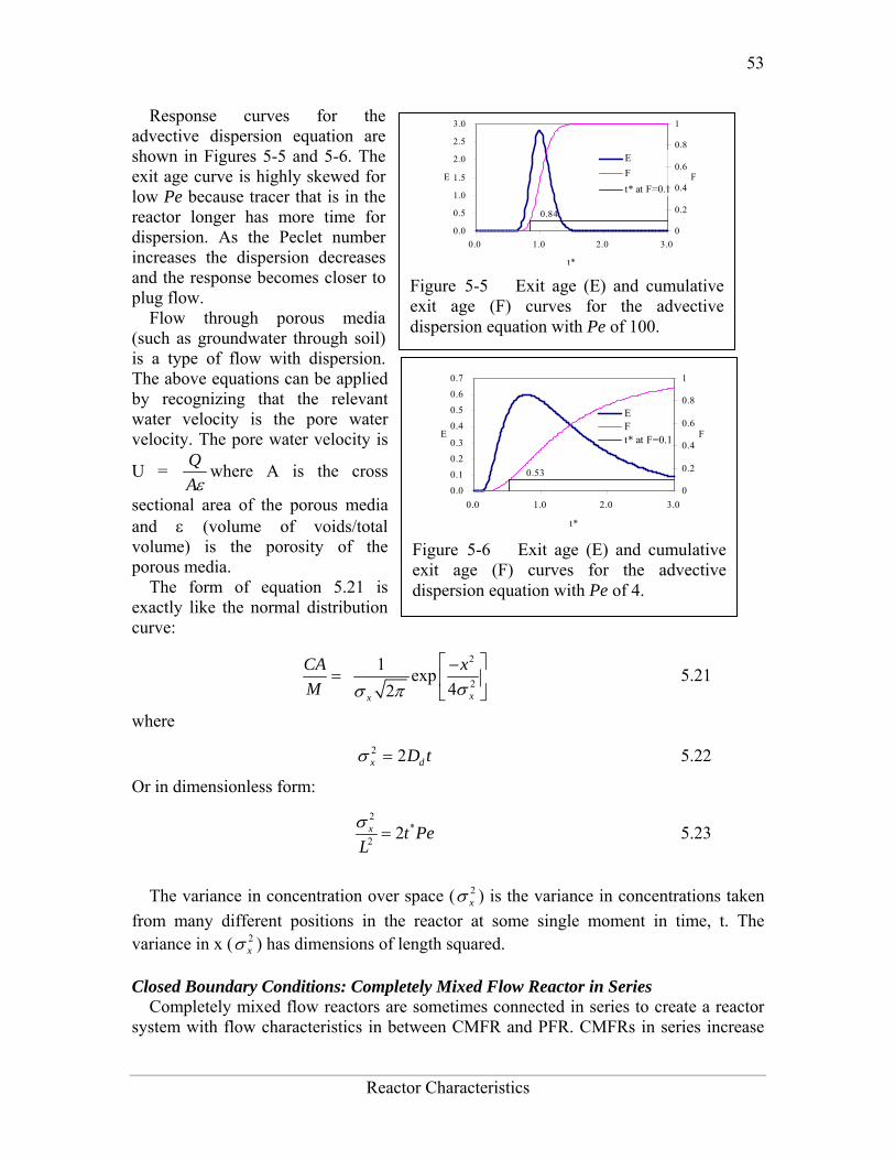
53


Response curves for the advective dispersion equation are shown in Figures 5-5 and 5-6. The exit age curve is highly skewed for low Pe because tracer that is in the reactor longer has more time for dispersion. As the Peclet number increases the dispersion decreases and the response becomes closer to plug flow.

Flow through porous media (such as groundwater through soil) is a type of flow with dispersion. The above equations can be applied by recognizing that the relevant water velocity is the pore water velocity. The pore water velocity is

U = QAε

where A is the cross

sectional area of the porous media and ε (volume of voids/total volume) is the porosity of the porous media.

The form of equation 5.21 is exactly like the normal distribution curve:

2

2

1 expxx

CA xM σσ π

⎡ ⎤−= ⎢ ⎥42 ⎣ ⎦

5.21

where

2 2x dD tσ = 5.22

Or in dimensionless form:

2

*2 2x t Pe

Lσ

= 5.23

The variance in concentration over space ( 2

xσ ) is the variance in concentrations taken from many different positions in the reactor at some single moment in time, t. The variance in x ( 2

xσ ) has dimensions of length squared.

Closed Boundary Conditions: Completely Mixed Flow Reactor in Series Completely mixed flow reactors are sometimes connected in series to create a reactor

system with flow characteristics in between CMFR and PFR. CMFRs in series increase

0.84

0.0

0.5

1.0

1.5

2.0

2.5

3.0

0.0 1.0 2.0 3.0

t*

E

0

0.2

0.4

0.6

0.8

1

F

EFt* at F=0.1

Figure 5-5 Exit age (E) and cumulative exit age (F) curves for the advective dispersion equation with Pe of 100.

0.53

0.00.10.20.3

0.40.50.60.7

0.0 1.0 2.0 3.0

t*

E

0

0.2

0.4

0.6

0.8

1

F

EFt* at F=0.1

Figure 5-6 Exit age (E) and cumulative exit age (F) curves for the advective dispersion equation with Pe of 4.

54


overall process efficiency because the reactants are at higher concentrations in the first reactors than they would be in a single large CMFR. Thus the total reactor volume can be smaller with a series of CMFRs. Similarly the reaction process can be made more efficient given the same reactor volume it if is divided into series CMFRs.

Non ideal reactors with mixing levels between that of CMFRs and PFRs and reactors containing baffles can also be modeled as a series of CMFRs. In this case the mixing level for the system is represented by the number of CMFRs that are used to represent the non-ideal reactor. The equation describing the concentration of a conservative tracer in the Nth reactor is given in equation 5.24.

( )( )

1

1 !

NtNNNC t N tM N e

θ

θ

−⎛ ⎞⎜ ⎟⎝ ⎠

−∀ ⎛ ⎞= ⎜ ⎟− ⎝ ⎠ 5.24

The non-dimensional form of equation 5.24 is given in equation 5.25

( ) ( ) ( )( )*

*

1*

1 !

NtN N

N t

NE tN e

−−=

− 5.25

It can be shown that equations 5.18 and 5.25 converge for large N when

2Pe N= 5.26 Equation 5.24 is limited to integral values of N. The model could be extended to

include non integral values of N if the factorial function were replaced with the Γ function. Note that the Γ function is not defined as an extension of the factorial function in Excel. Instead use the functions EXP(GAMMALN(N)) to calculate the Γ function.

Response curves for the advective dispersion equation are shown in Figure 5-7. Notice that the effluent concentration begins to rise much more quickly in series CMFRs than in the advective

dispersion model. This distinction between the two models lessens as the number of reactors increases and the Pe increases.

Reactor Studies

Measuring Reactor Characteristics One of the easiest methods to determine the mixing (dispersion) characteristics of a

reactor is to add a spike input of a conservative material and then monitor the

0.26

0.00.10.20.30.40.50.60.70.8

0.0 1.0 2.0 3.0

t*

E

0

0.2

0.4

0.6

0.8

1

FE

F

t* at F=0.1

Figure 5-7 Exit age (E) and cumulative exit age (F) curves for series CMFR with N of 2.

55


concentration of the material in the reactor effluent. The variance of tracer concentration versus time ( 2

tσ , with dimensions of time squared) can be measured by sampling at a single point in the reactor at many different times and can be computed using the following equations.

2 2

2 20 0

0 0

t

C t t t dt t C t dtt

C t dt C t dtσ

∞ ∞

∞ ∞

( )( − ) ⋅ ( ) = = −

( ) ( )

∫ ∫

∫ ∫ 5.28

where

0

0

( )

( )

t C t dtt

C t dt

∞

∞=∫

∫ 5.29

For discrete data points:

2

2 20

0

n

i ii

t n

ii

t C tt

C tσ =

=

⋅ ∆= −

∆

∑

∑ 5.30

and

0

0

n

i ii

n

ii

t C tt

C t

=

=

⋅ ∆=

∆

∑

∑ 5.31

Inlet and outlet boundary conditions affect the response obtained from a reactor. Closed reactors have little dispersion across their inlet and outlet boundaries whereas "open" reactors can have significant dispersion across their inlet and outlet boundaries. Typically open systems have no physical boundaries in the direction of flow. An example of an open system would be a river segment. Closed systems have small inlets and outlets that minimize dispersion across the inlet and outlet regions. An example of a closed system is a tank (or a lake) with a small inlet and outlet. The reactor used in the lab is closed. The t in equation 5.31 is the measured average residence time for the tracer in the reactor. For ideal closed reactors the measured residence time, t , is equal to the theoretical hydraulic residence time (θ = reactor volume/flow rate). For open reactors t can exceed the hydraulic residence time. If t is less than the hydraulic residence time it may indicate that the reactor contains “dead volume” or “short circuiting” such that some volume of the reactor is effectively unused.

56


The above equations suggest that from the reactor response to a spike input we can compute the dispersion coefficient for the reactor. We have two options for measuring reactor response: 1) synoptic measurements: at a fixed time sampling many points along the axis of the

reactor will yield a Gaussian curve of concentration vs. distance. In practice synoptic measurements are difficult because it requires sampling devices that are time-coordinated. By combining equations 5.22, 5.30, and 5.31 it is possible to estimate the dispersion coefficient from synoptic measurements.

2) single point sampling: measure the concentration at a fixed position along the x axis of the reactor for many times. If the reactor length is fixed at L and measurements are made at the effluent of the reactor (observe the concentration of a tracer at x = L as a function of time) then x is no longer a variable and C(x,t) becomes C(t) only. The response curve obtained through single point sampling is skewed. The curve “spread” changes during the sampling period and the response curve is skewed.

Peclet Number Estimation For single point sampling of the effluent response curve, skew increases as the

dispersion level in the reactor increases. The degree of skew depends on the dispersion coefficient, the velocity in the x-direction, and the length of the reactor. Peclet values in the range 100<Pe<∞ result in a symmetric response curve.

Response curve skew makes the assumption of a symmetrical normal distribution curve inappropriate and a new relationship between the variance and the dispersion coefficient (or Pe) has to be determined. Boundary conditions affect the determination of the dispersion coefficient. The relationship between the Peclet number and variance for open systems is given by:

2 22

2 8t Pe Pe

σ θ⎛ ⎞= + ⋅⎜ ⎟⎝ ⎠

5.33

For closed systems the relationship is:

( )2 22

2 2 1 Pet Pe Pe eσ θ−⎡ ⎤= − ⋅ − ⋅⎢ ⎥⎣ ⎦

5.34

The term 2Pe

in equations 5.33 and 5.34

is dominant for Peclet numbers much greater than 10 as is shown in Figure 5-8. The additional terms in equations 5.33 and 5.34 are corrections for skewedness in the response curve. These skewedness corrections are not very significant for Peclet numbers greater than 10. Thus for Peclet numbers greater than 10 the Peclet number can be determined using equation 5.35 for both open and closed systems.

10000

1000

100

10

1

0.1

0.01

0.0011000010001001010.10.010.001

Pe

2/Pe

open

closed

σ2

θ 2

Figure 5-8. Relationship between equations 5.33 through 5.34.

57


2

2

2

t

Pe θσ

= 5.35

Mass Conservation When a pulse of conservative tracer is added to a continuous flow reactor, all of the

tracer is expected to leave the reactor eventually. The mass of a substance that has left the reactor is given in equation 5.36.

0

n

out i ii

M QC t=

= ∆∑ 5.36

where Q is the flow rate and M is the mass of any substance whose concentration is given by C. If Q and ∆t are constant, then equation 5.36 can be rewritten as

0

n

out ii

M Q t C=

= ∆ ∑ 5.37

Equation 5.37 can be used to determine if all of the tracer was measured in the reactor effluent. Alternately, mass conservation can be checked by plotting the F curve and checking if the plot approaches 1. If some of the tracer is in the reactor at the end of the experiment then the following equation can be used to test for mass closure.

in out storedM M M= + ∆ 5.38

Tracers A conservative tracer will be used to characterize each of the reactors. Typical tracers

include salt and various dyes. For the experiment we will use hydrogen ions as the conservative tracer. Normally hydrogen ions would not be a good choice because they are reactive. In the laboratory we can circumvent that problem by using distilled water to eliminate potential reactants. The hydrogen ion concentration will be measured using a pH probe. The hydrogen ions will be added as hydrochloric acid.

A reasonable number of hydrogen ions to add can be calculated based on the following constraints. An excessively high concentration of hydrogen ions will cause low pH values that may not be measured accurately. Low concentrations of hydrogen ions will not be conservative because some reactions will occur with carbonates that have dissolved in the distilled water from the atmosphere. The concentration of total carbonates can be obtained by setting the ANC to zero and solving for pH, then solving for Ct. The concentration of bicarbonate, the only reactive species at low pH can be calculated based on the Ct and the pH. The concentration of bicarbonate is approximately 2.2 µM in distilled water. To reduce the error caused by reaction with bicarbonate the target hydrogen ion concentration should be at least 100x the bicarbonate concentration. Given these constraints a first guess for a reasonable number of hydrogen ions is that the hydrogen ion concentration of a completely mixed reactor containing the requisite tracer addition should be equivalent to pH 3.66 (or 220 µMoles H+ per liter of reactor).

Addition constraints for the tracer are that if a highly concentrated tracer is used, then there will be a significant density difference between the tracer and the water in the

58


reactor. If density matching is used to increase the density of the fluid in the reactor, then the high ionic strength of the reactor fluid will change the activity coefficient of H+. If a very dilute tracer is used then a large volume of tracer will need to be added and the volume of tracer could become a large fraction of the reactor volume and thus the pulse could no longer be modeled as having negligible volume.

Density Matching A common problem when using tracers is that the tracer may have a different density

than the fluid that is in the reactors. This is normally not a problem for reactors with low Peclet numbers or high levels of turbulence. However, density effects should not be overlooked since some of the tracer could easily sink to the bottom of the reactor and remain there. To compensate for the tracer density, the density of the water being pumped into the reactors will be increased by adding sodium chloride.

The solution density due to the addition of hydrochloric acid is approximately:

2

17.9solution H O HClNρ ρ= + 5.39

where HClN has units of eq/L and density is in kg/m3. The increase in density due to the addition of sodium chloride is approximately:

2

0.6985solution H O NaClCρ ρ= + 5.40

where NaClC has units of g/L. Equations 5.39 and 5.40 can be used to solve for the necessary concentration of NaCl given the tracer concentration of HCl.

25.6NaCl HClC N= 5.41

Activity Corrections When we measure pH we are actually measure the activity of the hydrogen ion, {H+}.

The true concentration, [H+], is equal to the activity divided by an activity coefficient.

[ ] { }CC

γ= 5.42

The activity coefficients for ions in an electrolyte are related to the concentration of ions. The ionic strength, µ, is defined as

212 i i

iC Zµ = ∑ 5.43

where iC is the molar concentration [moles/L] of the ith ion, Zi is its charge, and the summation extends over all of the ions in the solution. The activity coefficient, γ, is a nonlinear function of the ionic strength. Several relationships have been proposed. The Davies relationship for activity is valid for ionic strengths up to 0.5 M (see Figure 5-9).

59


20.2

2 110Z µµ

µγ⎛ ⎞

−⎜ ⎟⎜ ⎟+⎝ ⎠= 5.44

The activity coefficient correction is generally unnecessary for dilute solutions. However, in this laboratory we will use sodium chloride for density matching and the concentration of sodium chloride will be high enough that the activity of the hydrogen ions will be significantly decreased.

Acid Tracer Design The reactors are 30 cm long and

15 cm wide. If the depth is limited to 5 cm, then the total volume is 2.25 L and with the maximum pumping rate (380 mL/min) for our peristaltic pumps the residence time is 6 minutes. Acid tracer can be added as 0.05 M HCl. If the reactor volume is 2.25 L with 220 µeq/L of H+ then 500 µeq of H+ (or 10 mL 0.05 M HCl) are required.

The tracer can be poured directly into the first chamber of your reactor or it can be injected into the influent line. Red dye or methylene blue can also be added to the tracer or used separately to qualitatively observe the turbulence levels of the jets.

Mass balance Collect data that makes it possible to perform a mass balance on hydrogen ions. Note

that if it is expedient to shorten an experimental run such that there is a significant quantity of the tracer residual in the reactor, that the residual (stored) tracer can be measured by pouring the reactor contents into a container and measuring the pH of the resultant mixture.

Reactor Design

Baffle Design Baffles can be added to tanks to decrease the ability of the solution to travel quickly

from the tank inlet to the tank outlet. The goal of the baffle design depends on whether the tank is designed for a reaction or for separation. The baffles in reactors should generally be designed to achieve mixing in each of the baffled zones. The baffles in tanks designed for separation (clarifiers) should be designed to achieve uniform flow (a much more difficult goal to achieve). Mixing within each baffled zone could be achieved with a propeller mixer or by appropriately sized ports in the baffles. If port mixing is desired the energy for mixing is provided by the kinetic energy of the fluid flowing through the ports.

0.7

0.75

0.8

0.85

0.9

0.95

1

0.00001 0.001 0.1

ionic strength (moles/L)

activ

ity c

oeff

icie

nt

Figure 5-9. Activity coefficient as a function of ionic strength for ionic species with a charge of +/- 1 based on the Davies relationship (equation 5.44).

60


The flow characteristics of a baffled tank are complex and would require computational fluid dynamics to model. In lieu of developing a CFD model we will turn to dimensional analysis to help us characterize the mixing efficiency of a baffled reactor segment. The independent parameter that we will measure to characterize the reactor is its Peclet number.

The design goal is to determine the diameter and spacing of the ports required to achieve adequate mixing. The fluid flow out of the ports is jet flow. The jets entrain and mix with the surrounding fluid. To develop effective mixing the jet should be turbulent. The transition between turbulent and laminar behavior for jets occurs at a jet Reynolds number of a few hundred2.

Re jet jetjet

V dν

= or 4

Re jetjet

jet

Qdπ ν

= or 4Re reactorjet

ports jet

Qn dπ ν

= 5.46

The optimal port spacing for maximum mixing could be based on the spread of the jet in the distance to the next baffle. Jets expand in the radial direction at a rate of approximately 10% of the distance the jet travels axially. Thus the port spacing could be in a rectangular grid with the distance between ports equal to 10% of the distance between baffles. This spacing may be smaller than practical since it will require a large number of ports.

An additional constraint on port design is that the head loss through the ports not be excessive. The hydraulic grade line (and thus depth of each baffled reactor) will drop by a distance equal to the head loss through the ports. The head loss through the ports is given by the orifice equation

2orifice orifice orificeQ K A g h= ∆ 5.47

where the orifice coefficient, orificeK , has a value of approximately 0.6, the area of the orifice is orificeA , and the head loss through the orifice is h∆ .

2

24orifice

orifice orifice

dQ K g h

π= ∆ 5.48

2

24orifice

reactor orifice orifice

dQ n K g h

π= ∆ 5.49

where orificen is the number of ports. Solving for the port diameter we obtain.

4

2reactor

orificeorifice orifice

Qd

n K g hπ=

∆ 5.50

2Personal communication with Dr. Cowen.

61


Chlorine Contact Tank Design The design objective for chlorine contact tanks is to maximize the inactivation of

pathogens by maximizing the contact time between the chlorine and the pathogens before the water is sent to the distribution system. This objective has been codified with the contact time for a tank defined as the time for the effluent of the tank to reach 10% of the influent value after a step change in the influent.

Table 5-1. Comparison of * 0.1t at F = for non-ideal reactors (Malcolm Pirnie, 1991) Baffling Condition

Guidance manual value of

* 0.1t at F =

Extent of Baffles

Unbaffled (CMFR)

0.1 No baffles, agitated basin with low length to width ratio, high inlet and outlet flow velocities

Poorly baffled 0.3 Single or multiple unbaffled inlets and outlets, no intrabasin baffles

Average 0.5 Baffled inlet or outlet with some intrabasin baffles Superior 0.7 Perforated inlet baffles, serpentine or perforated

intrabasin baffles, outlet weir or perforated launders Perfect (PFR) 1.0 Very high length to width ratio (pipeline flow),

perforated inlet, outlet and intrabasin baffles

Procedures The reactor you

will be working with can be easily modified by installing various configurations of perforated baffles (Figure 5-10). Your objectives are

• to modify the reactor to obtain a maximum value of * 0.1t at F =

• to document your progress toward this goal by obtaining appropriate experimental data

• to compare your experimental data with appropriate models Note that you are allowed to collaborate with other teams to obtain the results from

additional tests. All data sharing must be documented in your report.

Baffle installation The baffles can be installed by rolling a 3 mm diameter roll of putty and applying the

putty to the bottom and one side of the baffle. Carefully install the baffle by rotating it

Figure 5-10 Perforated baffle designs. The hole patterns are designed to create different levels of mixing and to create serpentine flow paths.

62


into place (so the putty on the one side doesn’t have to slide) and then pressing it down (so the putty on the bottom doesn’t have to slide). Install the two bolts with wing nuts to hold the baffle in place. Add a roll of putty to the corner formed at the unsealed side of the baffle and press the putty into place.

Testing protocol To establish the steady-state hydraulic profile of your reactor it will be necessary to

operate at normal flow for a minute or more prior to injecting the tracer. The reactor volume can be adjusted by changing the reactor effluent weir height. Data collection can be by the pH meter software or by the Process Controller. The flow rate can also be varied. When choosing flow rates, consider that it will be necessary to run tests for several hydraulic residence times. As part of your experimental protocol ensure you have all of the necessary data for analysis including flow rates, tracer volumes, tracer concentration, reactor volumes, and tracer injection times.)

To ensure that everything is working properly I recommend that you begin by first testing a CMFR. Use the CMFR data to verify that you obtain mass balance and that you obtain the expected exit age response.

For each test make sure that you accurately measure the reactor volume, residual reactor pH, and the flow rate. The reactor volume should be measured by pouring the reactor contents into another container and then using the 5k electronic balance to determine the volume of water. Measure the residual concentration of hydrogen ions in the reactor by measuring the pH of the container contents. The flow rate can be accurately measured by massing an accurately timed sample from the pump (not from the reactor effluent).

The pH probes are extremely sensitive to voltage fluctuations. The peristaltic pumps produce small amounts of static electricity as the rollers squeeze over the pump tubing. The result is a small change in voltage level of the solution in the reactor. This voltage fluctuation will be picked up by the pH probe and cause poor quality data. To eliminate this problem a small grounding rod should be installed in the reactor and connected to an electrical ground. The stirrer housing is grounded and thus any metal that is directly connected to the stirrer housing is grounded. An alternate way to ground the reactor solution is to have the water flow through a short section of grounded metal tubing.

Prelab Questions 1) Calculate the concentration of bicarbonates in distilled water in equilibrium with the

atmosphere. (This is similar to the Gran Plot prelab requiring the use of Solver.) 2) Calculate the change in hydraulic grade line between baffled sections of a reactor

with a flow rate of 300 mL/min. The reactor baffles are perforated with 24 holes 1 mm in diameter.

3) Calculate the concentration of hydrogen ions in the reactor effluent given the following situation. You added enough NaCl to the distilled water flowing through the reactor to match the density of 0.05 N HCl. You measured the pH in the reactor effluent to be 4.0. (Hint: the activity of the hydrogen ions is less than 1.)

63


Data Analysis Use a consistent set of units throughout your data analysis and include the units in your

spreadsheet and report! 1) Convert the pH measurements into proton concentration including the correction for

activity.

2) Create the data E curve from ( )( )*

*

rt

ttr

CE

M

∀= .

3) Create model E curves for CMFR in series and for the one dimensional advective dispersion equation.

4) Use multivariable nonlinear regression to obtain the best fit between the model E curves and the data E curve by using Solver to minimize the sum of the squared errors. Allow Solver to vary the values of θ, trM , and either N or Pe (depending on the model).

5) Compare trM obtained using Solver with the actual trM added and comment on any differences.

6) Compare θ obtained using Solver with the measured value of θ and comment on any differences.

7) Plot data and model E curves and if appropriate show both model E curves and explain which model fits best and compare with your expectations.

8) Evaluate whether there is any evidence of “dead volumes” or “short circuiting” in your reactor.

9) Make a recommendation for the design of a full scale chlorine contact tank. As part of your recommendation discuss the following: • Serpentine flow paths versus perforated baffled reactors. • Effects of scaling up to full size based on dimensional analysis. • Effects of Reynolds scale effects on modeling baffled and serpentine flow. • Cumulative head loss through the contact tank.

References Weber, W. J. J. and F. A. Digiano. 1996. Process Dynamics in Environmental Systems.

New York, John Wiley & Sons, Inc. Malcolm Pirnie, Inc., and HDR Engineering, Inc. “Guidance Manual for Compliance

with the Filtration and Disinfection Requirements for Public Water Systems Using Surface Water Sources.” AWWA, Denver CO, 1991.

64


Lab Prep Notes


number reactor with

baffles CEE shop

variable flow digital drive


Easy-Load pump head


PharMed tubing size 18


20 liter HDPE Jerrican

Fisher Scientific 02-961-50C

Table 5-3. Reagent list Description Supplier/Source Catalog

number Acid tracer 0.5 N HCl red dye #40 MG Newell 07704-1

1) Use # 18 tubing for baffled tank. 2) Organize team research so they don’t use the same materials and so they answer

different questions.

65

Gas Transfer

Gas Transfer

Introduction Exchange of gases between aqueous and gaseous phases is an essential element of

many environmental processes. Wastewater treatment plants require enhanced transfer of oxygen into activated sludge tanks to maintain aerobic degradation. Water treatment plants require gas transfer to dissolve chlorine gas or ozone. Gas transfer can also be used to remove unwanted volatile chemicals such as carbon tetrachloride, tetrachloroethylene, trichloroethylene, chloroform, bromdichloromethane, and bromoform from water (Zander et al., 1989). Exchange of a dissolved compound with the atmosphere is controlled by the extent of mixing in the aqueous and gaseous phase, the surface area of the interface, the concentration of the compound in the two phases, and the equilibrium distribution of the compound. Technologies that have been developed to enhance gas transfer include: aeration diffusers, packed-tower air stripping, and membrane stripping. Each of these technologies creates a high interface surface area to enhance gas transfer.

Theory Oxygen transfer is important in many environmental systems. Oxygen transfer is

controlled by the partial pressure of oxygen in the atmosphere (0.21 atm) and the corresponding equilibrium concentration in water (approximately 10 mg/L). According to Henry’s Law, the equilibrium concentration of oxygen in water is proportional to the partial pressure of oxygen in the atmosphere.

Natural bodies of water may be either supersaturated or undersaturated with oxygen depending on the relative magnitude of the sources and sinks of oxygen. Algae can be a significant source of oxygen during active photosynthesis and can produce supersaturation. Algae also deplete oxygen levels during the night.

At high levels of supersaturation dissolved gas will form microbubbles that eventually coalesce, rise, and burst at the water surface. The bubbles provide a very efficient transfer of supersaturated dissolved gas to the gaseous phase, a process that can be observed when the partial pressure of carbon dioxide is decreased by opening a carbonated beverage. Bubble formation by supersaturated gasses also occurs in the environment when cold water in equilibrium with the atmosphere is warmed rapidly. The equilibrium dissolved oxygen concentration decreases as the water is warmed (Figure 6-1).

Supersaturation of dissolved gases can also occur when water carrying gas bubbles from a water fall or spillway plunges into a

6789

101112

10 20 30 40

Temperature (°C)

Oxy

gen

(ppm

)

Figure 6-1. Dissolved oxygen concentrations in equilibrium with the atmosphere.

66


deep pool. The pressure increases with depth in the pool and gasses carried deep into the pool dissolve in the water. When the water eventually approaches the surface the pressure decreases and the dissolved gases come out of solution and form bubbles. Bubble formation by supersaturated gases can kill fish (similar to the “bends” in humans) as the bubbles form in the bloodstream.

Gas Transfer Coefficient Gas transfer rate can be modeled as the product of a driving force (the difference

between the equilibrium concentration and the actual concentration) and an overall volumetric gas transfer coefficient (a function of the geometry, mixing levels of the system and the solubility of the compound). In equation form

( )*,v̂ l

dC k C Cdt

= − 6.1

where C is the dissolved gas concentration, C* is the equilibrium dissolved gas concentration and ,v̂ lk is the overall volumetric gas transfer coefficient . Although ,v̂ lk has dimensions of 1/T, it is a function of the interface surface area (A), the liquid volume (V), the oxygen diffusion coefficient in water (D), and the thickness of the laminar boundary layer (δ) through which the gas must diffuse before the much faster turbulent mixing process can disperse the dissolved gas throughout the reactor.

,ˆ ( , , , )v lk f D A Vδ= 6.2

The overall volumetric gas transfer coefficient is system specific and thus must be evaluated separately for each system of interest (Weber and Digiano, 1996).

A schematic of the gas transfer process is shown in Figure 6-2. Fickian diffusion controls the gas transfer in the laminar boundary layer. The oxygen concentration in the bulk of the fluid is assumed to be homogeneous due to turbulent mixing and the oxygen concentration above the liquid is assumed to be that of the atmosphere.

The gas transfer coefficient will increase with the interface area and the diffusion coefficient and will decrease with the reactor volume and the thickness of the boundary layer. The functional form of the relationship is given by

,v̂ lADkVδ

= 6.3

Equation 6.1 can be integrated with appropriate initial conditions to obtain the

concentration of oxygen as a function of time. However, care must be taken to ensure that

δ

oxygen gas

dissolv edoxygenV/ A

CC*

Figure 6-2. Single film model of interphase mass transfer of oxygen.

67

Gas Transfer

the overall volumetric gas transfer coefficient is not a function of the dissolved oxygen concentration. This dependency can occur where air is pumped through diffusers on the bottom of activated sludge tanks. Rising air bubbles are significantly depleted of oxygen as they rise through the activated sludge tank and the extent of oxygen depletion is a function of the concentration of oxygen in the activated sludge. Integrating equation 6.1 with initial conditions of C = C0 at t = t0

0 0

,*ˆ

C t

v lC t

dC k dtC C

=−∫ ∫ 6.4

*

, 0*0

ˆln ( )v lC C k t tC C

−= − −

− 6.5

Equation 6.5 can be evaluated using linear regression so that ,v̂ lk is the slope of the line. The simple gas transfer model given in equation 6.5 is appropriate when the gas

transfer coefficient is independent of the dissolved gas concentration. This requirement can be met in systems where the gas bubbles do not change concentration significantly as they rise through the water column. This condition is met when the water column is shallow, the bubbles have large diameters, or the difference between the concentration of dissolved gas and the equilibrium concentration is small.

Oxygen Transfer Efficiency An important parameter in the design of aeration systems for the activated sludge

process is the energy cost of compressing air to be pumped though diffusers. The pumping costs are a function of the pressure and the airflow rate. The pressure is a function of the hydrostatic pressure (based on the depth of submergence of the diffusers) and the head loss in the pipes and through the diffuser. The required airflow rate is a function of the BOD of the wastewater and the efficiency with which oxygen is transferred from the gas phase to the liquid phase. This oxygen transfer efficiency (OTE) is a function of the type of diffuser, the diffuser depth of submergence, as well as temperature and ionic strength of the activated sludge. Oxygen transfer is a remarkably inefficient process; only a small fraction of the oxygen carried by the rising bubbles diffuses into the activated sludge. The most efficient systems use membrane diffusers and achieve an OTE of approximately 10%.

The manufacturer typically provides oxygen transfer efficiency for a specific diffuser. In this laboratory we will measure oxygen transfer efficiency for the aeration stone that we will be using in an activated sludge tank. The molar transfer rate of oxygen through the diffuser is

2

2

air air Ogas o

Q P fn

RT= 6.6

where 2Of is the molar fraction of air that is oxygen (0.21), airQ is the volumetric flow

rate of air into the diffuser, airP is the air pressure immediately upstream from the diffuser, R is the universal gas constant and T is absolute temperature. If the airflow rate is

68


already given with units of moles/s then the molar transfer rate of oxygen can be obtained by multiplying by the molar fraction of air that is oxygen.

The molar rate of dissolution into the aqueous phase is

2

2

aq oO

V dCnMW dt

= 6.7

where 2OMW is the molecular weight of oxygen, V is the reactor volume, and dC

dtis the

change in aqueous oxygen concentration with time. The rate of change of oxygen concentration is a function of the dissolved oxygen concentration and is a maximum when the dissolved oxygen concentration is zero. Oxygen transfer efficiency could be measured for any dissolved oxygen concentration. A better method of analysis is to

substitute the right side of equation 6.1 for dCdt

.

( )

2

2

*,v̂ l

aq oO

Vk C Cn

MW−

= 6.8

The oxygen transfer efficiency is the ratio of equation 6.8 to equation 6.6.

( )

2 2

*,v̂ l

O air air O

k C C VRTOTE

MW Q P f−

= 6.9

Measurement of OTE using equation 6.9 requires that the gas transfer coefficient, air flow rate, air pressure, and the air temperature be measured. (Pair and Qair have to correlate and in this experiment the best combination is atmospheric pressure and the flow rate given by the pump.)

If the molar airflow rate is controlled then OTE is based on the ratio of equation 6.8 to the molar transfer rate of supplied oxygen.

( )

2

2 2 2

*,v̂ laq o

O air O air O

Vk C CnOTE

f n f n MW

−= = 6.10

Deoxygenation To measure the reaeration rate it is necessary to first remove the oxygen from the

reactor. This can be accomplished by bubbling the solution with a gas that contains no oxygen. Nitrogen gas is typically used to remove oxygen from laboratory reactors. Alternately, a reductant can be used. Sulfite is a strong reductant that will reduce dissolved oxygen in the presence of a catalyst.

cobalt2 22 3 4O 2SO 2SO− −+ ⎯⎯⎯→ 6.11

The mass of sodium sulfite required to deoxygenate a mg of oxygen is calculated from the stoichiometry of equation 6.11.

69

Gas Transfer

2 3 2 3 2 32

2 2 2 3 2

2 mole Na SO 126,000 mg Na SO 7.875 mg Na SOmole O32000 mg O mole O mole Na SO mg O

⋅ ⋅ = 6.12

If complete deoxygenation is desired a 10% excess of sulfite can be added. The sulfite will continue to react with oxygen as oxygen is transferred into the solution. The oxygen concentration can be measured with a dissolved oxygen probe or can be estimated if the temperature is known and equilibrium with the atmosphere assumed (Figure 6-1).

Experimental Objectives The objectives of this lab are to:

1) Illustrate the dependence of gas transfer on gas flow rate. 2) Develop a functional relationship between gas flow rate and gas transfer. 3) Measure the oxygen transfer efficiency of a course bubble diffuser. 4) Explain the theory and use of dissolved oxygen probes. See

http://ceeserver.cee.cornell.edu/mw24/Labdocumentation/sensors.htm for information on how the dissolved oxygen probe works.

A small reactor that meets the conditions of a constant gas transfer coefficient will be used to characterize the dependence of the gas transfer coefficient on the gas flow rate through a simple diffuser. The gas transfer coefficient is a function of the gas flow rate because the interface surface area (i.e. the surface area of the air bubbles) increases as the gas flow rate increases.

Experimental Methods The reactors

are 4 L containers (Figure 6-3). The DO probe should be placed to minimize the risk of air bubbles lodging on the membrane on the bottom of the probe. The aeration stone is connected to a source of regulated air flow. A 7-kPa pressure sensor (optional) can be used to measure the air pressure immediately upstream from the diffuser stone. A 200-kPa pressure sensor is used to measure the air pressure in the accumulator.

S 1

Air Supply

N 2

DO probe

Stir bar

Temperature probe(optional)



Accumulator7 kPa Pressure sensor (optional)

S 2

1.5 mm ID x 5 cm restriction

S 1S 1

Air Supply

N 2N 2

DO probe

Stir bar

Temperature probe(optional)



Accumulator7 kPa Pressure sensor (optional)

S 2S 2

1.5 mm ID x 5 cm restriction

Figure 6-3. Apparatus used to measure reaeration rate.

http://ceeserver.cee.cornell.edu/mw24/Labdocumentation/sensors.htm

70


Initial Setup

1) Assemble the apparatus (don’t forget the 1.5 mm x 5 cm restriction). 2) Install a membrane on the oxygen probe. 3) Add 4 L of tap water to the reactor. 4) Open the Process Controller software. 5) Configure the Process Controller software

(http://ceeserver.cee.cornell.edu/mw24/cee453/NRP/configure_PC.htm) 6) Set the Process Controller to Automatic Operation. 7) Set the state to “prepare to calibrate.” The process controller should quickly cycle

through the calibration step and then begin attempting to control the air flow rate to the target value.

8) Set the stirrer speed to 5. 9) Calibrate the DO probe (See

http://ceeserver.cee.cornell.edu/mw24/Software/DOcal.htm). Use 22ºC as the temperature.

10) Add 10 mg CoCl2· 6H2O (note this only needs to be added once because it is the catalyst). A stock solution of CoCl2· 6H2O (100 mg/mL – thus add 100 µL) has been prepared to facilitate measurement of small cobalt doses. (Use gloves when handling cobalt!)

Test the air flow controller In the following test the air flow controller should provide a constant flow of air into

the accumulator. You can assess how well the air flow controller is working based on the slope of the pressure as a function of time. 1) Set the Process Controller to “Manual Locked in State.” 2) Set the state to off 3) Open the accumulator cap to empty the accumulator. 4) Close the accumulator cap. 5) Close the needle valve. 6) Set the air flow rate to 200 µM/s. 7) Begin logging data at 1 s interval using the datalog button on the plant operation tab.

Data is being logged when the icon is green. 8) Set the state to aerate. 9) End logging data when the accumulator pressure is approximately equal to the source

pressure. 10) Analyze the data to see if the airflow rate is close to the expected value. If the error is

greater than 20% look for leaks and recalibrate the airflow controller.

http://ceeserver.cee.cornell.edu/mw24/cee453/NRP/configure_PC.htm

http://ceeserver.cee.cornell.edu/mw24/Software/DOcal.htm

71

Gas Transfer

Measure the Gas Transfer

1) Prepare to record the dissolved oxygen concentration using the Process Control software. Use 5-second data intervals and log the data to \\Enviro\enviro\Courses\453\your folder\gastran\ for later analysis. Include the flow rate in the file name.

2) Set the airflow rate to the desired flow rate. 3) Set the state to aerate. 4) Set the needle valve so the pressure in the accumulator is approximately 75% of the

source pressure. 5) Wait until the accumulator pressure reaches steady state. 6) Turn the air off by changing the operator selected state to “OFF.” 7) Add enough sodium sulfite to deoxygenate the solution. A stock solution of sodium

sulfite (100 mg/mL) has been prepared to facilitate measurement of small sulfite doses. Calculate this dose based on the measured dissolved oxygen concentration. (4 L of water at Coxygen mg O2/L = 4 Coxygen mg O2, therefore add 4(7.875)(Coxygen) mg sodium sulfite or 4(7.875)(Coxygen)/100 mL of stock solution.)

8) Turn the air on by changing the operator selected state to “Aerate.” 9) Monitor the dissolved oxygen concentration until it reaches 50% of saturation value

or 10 minutes (whichever is shorter). 10) Repeat steps 1-9 to collect data from additional flow rates. 11) Consolidate the files into one spreadsheet file with a separate sheet for each flow rate.

Prelab Questions 1) Calculate the mass of sodium sulfite needed to reduce all the dissolved oxygen in 4 L

of pure water in equilibrium with the atmosphere and at 30°C. 2) Sketch your expectations for dissolved oxygen concentration as a function of time for

the flow rates used on a single graph. The graph can be done by hand and doesn’t need to have any numbers on the time scale.

3) Why is ,v̂ lk not zero when the gas flow rate is zero? How can oxygen transfer into the reactor even when no air is pumped into the diffuser?

4) Sketch your expectations for ,v̂ lk as a function of gas flow rate. Do you expect a straight line? Why?

5) Read http://ceeserver.cee.cornell.edu/mw24/cee453/NRP/Airflow%20Control.doc. Does the air flow controller control the airflow into the accumulator or out of the accumulator?

Data Analysis This lab requires a significant amount of repetitive data analysis. Plan how you will

organize your spreadsheet to make the analysis as easy as possible.

http://ceeserver.cee.cornell.edu/mw24/cee453/NRP/Airflow Control.doc

72


1) Calculate the air flow rate from testing the air flow controller and compare with the target value.

2) Eliminate the data from each data set when the dissolved oxygen concentration was less than 0.5 mg/L. This will ensure that all of the sulfite has reacted.

3) Plot a representative data set showing dissolved oxygen vs. time. 4) Calculate *C for based on the average water temperature, barometric pressure,

and the following equation. 2

1727 2.105* TOC P e⎛ ⎞−⎜ ⎟⎝ ⎠= where T is in Kelvin,

2OP is the

partial pressure of oxygen in atmospheres, and *C is in mg/L. This equation is valid for 278 K<T<318 K.

5) Estimate ,v̂ lk using linear regression and equation 6.5 for each data set. Use the slope function in Excel; don’t use the equation displayed on the trendline plot!

6) Create a graph with a representative plot showing the linearized data, *

*0

ln C CC C

⎛ ⎞−⎜ ⎟−⎝ ⎠

vs. time, and the best-fit line.

7) Plot ,v̂ lk as a function of airflow rate (µmole/s).

8) Plot the reaeration model on the same graph as the data. 9) Look at each dataset and if necessary eliminate more data from the beginning (or

end) of the dataset. You will be able to see when the oxygen level is affected by residual sulfite at the beginning of the experiments.

10) Plot OTE as a function of airflow rate (µmole/s) with the oxygen deficit ( *C C− ) set at 6 mg/L.

11) Plot the oxygen dissolution rate (µmole/s) as a function of the air supply rate (µmole/s).

12) If the wastewater BOD is 325 mg/L and the wastewater flow rate is 16 L/day, what combination of airflow rate and diffusers would you use? You may assume that the entire BOD is consumed in the activated sludge tank, that *C for the wastewater is 8 mg/L and that the target dissolved oxygen concentration in the tank is 2 mg/L.

13) Comment on results and compare with your expectations and with theory. 14) Verify that your report and graphs meet the requirements. Check the course

website for details. (http://www.cee.cornell.edu/mw24/cee453/Lab_Reports/editing_checklist.htm and (http://www.cee.cornell.edu/mw24/cee453/Lab_Reports/default.htm)

References Weber, W. J. J. and F. A. Digiano. 1996. Process Dynamics in Environmental Systems.

New York, John Wiley & Sons, Inc. Zander, A. K.; M. J. Semmens and R. M. Narbaitz. 1989. “Removing VOCs by

membrane stripping” American Water Works Association Journal 81(11): 76-81.

http://ceeserver.cee.cornell.edu/mw24/cee453/Lab_Reports/editing_checklist.htm

http://www.cee.cornell.edu/mw24/cee453/Lab_Reports/default.htm

73

Gas Transfer

Lab Prep Notes

Setup

1) Prepare the sodium sulfite immediately before class and distribute to groups in 15 mL PP bottles to minimize oxygen dissolution and reaction with the sulfite.

2) The cobalt solution can be prepared anytime and stored long term. Distribute to student stations in 15 mL PP bottles.

3) Verify that DO probes, membranes, and potassium chloride solutions are available at each station. Students will install the membranes.

4) Verify that the top row of ports has a maximum voltage of 0.5 volts and that middle row of ports has a maximum voltage of 0.1 volts.

5) Provide clamps to mount DO probes on magnetic stirrers.

Major elements of apparatus • air flow hardware (built by

students) • reactor hardware (built by

students) • sensors (plugged in to ports by

TA) • solenoid valves (already plugged

in to ports by TA) • software

Class Plan

1) Show how to install membrane on DO probe. 2) Show how to calibrate DO probe using Calibrator. 3) Assign flow rates to teams. 4) Place all pH probes in buffer 4 so they are conditioned.

Table 6-1. Reagent list Description Supplier Catalog

number Na2SO3 Fisher Scientific S430-500

CoCl2· 6H2O Fisher Scientific C371-100

Table 6-2. Stock solutions list reagent M.W. g/100

mL mg/ mL

mL/ group

solubility g/L

Na2SO3 126.04 10 g 100 10 125 CoCl2· 6H2O

237.92 10 g 100 1 770


number magnetic stirrer Fisher Scientific 11-500-7S

100-1095 µL pipette


10-109.5 µL pipette


15 mL PP bottles

Fisher Scientific 02-923-8G

Solenoid valves Stamp control

boxes

Pressure sensors 1 L airflow

accumulators

Bench Flows (µM/s) 1 50, 100, 150 2 200, 250, 300 3 350, 400, 450 4 500, 600, 700 5 800, 900, 1000 6 1200, 1500, 2000 7 2500, 3000, 3500 8 4000, 4500, 5000

74


Volatile Organic Carbon Contaminated Site Assessment

Introduction Roughly 75 percent of the major cities in the U.S. depend, at least in part, on

groundwater for their water supply. Various estimates of the nationwide extent of groundwater contamination are stated to range from one to over two percent of the nation's usable groundwater (Council on Environmental Quality, 1981). Volatile organic compounds (VOCs) are the most frequently detected organic pollutants of groundwater in the United States. In fact, the VOCs are so ubiquitous that their analysis has been considered by the U.S. Environmental Protection Agency as a screening procedure to establish the need for more extensive characterization of groundwater samples from hazardous waste disposal sites. In the upstate region of New York (excluding Long Island), of approximately 570 groundwater contamination incidents reported by 1985, 98% involved either the volatile components of gasoline and petroleum or solvents and degreasers (NY State DEC, 1985).

Volatile organics may be transported in the subsurface as dissolved components in groundwater. However, by virtue of their volatility, VOCs will also exist in the gas phase of unsaturated porous media. As a result, volatile contaminants can be transported by advection and diffusion in the vapor phase. VOC transport processes are illustrated in Figure 7-1.

Experiment Description Students will use

soil gas sampling to prospect for a VOC that has leaked from a subsurface source into an unsaturated soil system. A rectangular “soil box” contaminated with a combination of liquid acetone, octane and toluene will be used. A soil with high organic content (potting soil) or low organic content (sand) may be used as the box filling material (porous medium). The VOCs will be identified and measured using a gas

Spill, or Leaky Storage Tanks

Vadose Zone

VOC loss to the atmosphere

Groundwater Flow

VOC movement as a Non Aqueous Phase Liquid (NAPL)

VOC movement as a gas in soil pores

VOC movement as a solute dissolved in groundwater

Figure 7-1. Subsurface VOC transport processes. The vadose zone is the region of the soil profile in which some pores contain gas and are therefore, unsaturated.

75


chromatograph (GC).

Experimental Procedures

Calibration (Peak Times) Each compound will have a unique retention time in the gas chromatograph. The time

for each of the 3 VOC peaks can be obtained by injection of 100 µl head space samples from crimp cap sealed vials containing a small volume liquid acetone, octane, and toluene. Use the syringe technique described below. Analyze each compound 4 times (12 samples) using a gas chromatograph (see http://ceeserver.cee.cornell.edu/mw24/Software/gas_chromatograph.htm for information on using the gas chromatograph). These analyses will also serve to “calibrate” the GC by generating the peak area that corresponds to the saturated vapor concentration. Gas chromatogram peak areas may be assumed to be directly proportional to the mass of vapor injected.

Syringe technique for sampling vial headspace The purpose of this syringe technique is to minimize the effects of sorption to the

Teflon and glass surfaces in the syringe and to eliminate carryover of sample in the needle. Using separate needles to collect samples and to inject into the GC eliminates needle carryover of sample. 1) Remove GC needle. 2) Purge syringe 5 times with room air to remove any residual VOCs. 3) Put on sample needle. 4) Insert into sample bottle (with syringe at zero volume) 5) Fill syringe fully with gas, wait 4 seconds, and purge syringe contents back into the

source bottle (repeat 3 times). 6) Fill syringe and adjust to 100 µL. 7) Close syringe valve and remove syringe from sample vial and remove sample needle. 8) Put on GC needle. 9) Instruct GC to measure sample. 10) Insert needle in injection port, open syringe valve, inject sample, hit start button (or

Enter) all as quickly as possible. 11) Remove syringe from the GC injection port.

Soil Gas Sampling See Table 7-1 for physical properties of the VOCs. See Tables 7-2, 7-3, and 7-4 (in the Lab Prep Notes) for necessary reagents, equipment and GC method. Prior to the laboratory the instructor will create a “spill” of a VOC by injecting 10 mL of liquid of two or more NAPLs into the “soil box” to be sampled by students. During the lab

http://ceeserver.cee.cornell.edu/mw24/Software/gas_chromatograph.htm

76


students will analyze approximately 50 soil gas samples from the “soil box” using the syringe technique outlined below. Results from the soil box analyses may be mapped using units of concentration (g/m3).

Syringe technique for soil gas sampling 1) Remove GC needle. 2) Purge syringe 10 times with room air to remove any residual VOCs. 3) Put on sample needle. 4) Insert into soil bed (with syringe at zero volume). 5) Fill syringe and adjust to 100 µl. 6) Close syringe valve, remove syringe from soil bed and remove sample needle. 7) Put on GC needle. 8) Instruct GC to measure sample (using software). 9) Insert needle in injection port, open syringe valve, inject sample, hit the enter key (or

OK) all as quickly as possible. 10) Remove syringe from the GC injection port.

Analysis of Soil Gas Sampling Students will use their analysis of VOC standards to obtain the corresponding GC

retention times and use this information to identify the unknown VOCs in the contaminated soil box. The vapor pressure and ideal gas law are used to estimate the mass of each compound present in the samples used to calibrate the GC.

PVnRT

= 7.1

where n is the number of moles of the compound, P is the vapor pressure of the compound [kPa], V is the syringe volume [L], R is the Gas Constant (8.31 [ ] [ ]L kPa mol K⋅ ⋅ ), and T is the temperature of the gas in the syringe [K]. The relationship between peak area (as measured by the GC) and mass of the compound is determined from the calibration.

Soil gas concentrations should be reported and plotted as contour lines on a map of the soil box (see Figure 7-2 for an illustration).

Table 7-1. Physical data for octane, acetone, and

Octane Acetone Toluene Solubility (g/m3) 0.6 very 515

Vapor Pressure (kPa) 1.88 (1.47) 24 3.8 (2.9) H (kPa m3/mol) 300 0.0159 0.67

GLH (g/L)/(g/L) 123 0.0065 0.275

Molecular Formula CH3(CH2)6CH3 CH3COCH3 C6H5CH3 Molecular weight 114.23 58.08 92.14

density (g/mL) 0.71 0.7857 0.8669

77


Procedure (short version) 1) Instructor will demonstrate syringe

technique (be careful not to pull plunger out of barrel) and Gas Chromatograph technique.

2) “Calibrate” GC by analyzing 4 samples for each VOC.

3) Take soil gas samples. 4) Convert the soil gas peak areas to

concentrations (g/m3). This data will be shared between groups.

5) Clean plasticware.

Prelab Questions 1) How are the identities of the

chromatogram peaks determined when using a gas chromatograph?

2) Explain why different needles are used for sampling from source vials and injecting the sample into the GC. Consider the temperature of the injection port (see Table 7-4) and the fact that these compounds absorb to most surfaces.

Data Analysis 1) Calculate the mass of each VOC in 100 µL of headspace of vials containing liquid

VOC. 2) Calculate the concentration of saturated vapor for each compound in g/m3. 3) Plot isoconcentration lines of the identified VOCs (expressed as gas concentration in

g/m3) on maps of the contaminated site (see Figure 7-2 for example). Prepare a map for each compound showing isoconcentration lines. (The Excel 3-D surface plot with contour lines can be used. Note that the grid needs to have uniform distance between samples for the Excel 3-D surface plot to work correctly.)

4) Compare the saturated vapor concentration with the peak concentration observed in the “sand box.”

References Ashworth, R. A., G. B. Howe, and T. N. Rogers. “Air-Water Partitioning Coefficients of

Organics in Dilute Aqueous Solutions.” J. Hazard. Mater. 18, p. 25-36, 1988. Council on Environmental Quality, "Contamination of Groundwater by Toxic Organic

Chemicals", 1981. Hwang, Y., J. D. Olson, and G. E. Keller, II, “Steam Stripping for Removal of Organic

Pollutants from Water. 2. Vapor-Liquid Equilibrium Data.” Ind. Eng. Chem. Res. 31, p. 1759-1768, 1992.

VOC NAPL source #2

VOC NAPL source #1

Sand

Sample grids

Figure 7-2. Students will prepare a map of the surface of their soil box. The map will show isoconcentration lines for each VOC.

78


Mackay, D. and W. Y. Shiu, “A Critical Review of Henry’s Law Constants for Chemicals of Environmental Interest”, J. Phys. Chem. Ref. Data. 10, p. 1175-1199, 1981.

New York State Department of Environmental Conservation, "Draft Upstate New York Groundwater Management Program", N.Y.S.D.E.C., Division of Water, Draft Report WM P-94, January, 1985.

79


Lab Prep Notes

Setup

1) Prepare 1 soil box under fume hood. 2) Moisten the sand but not so much that

there is standing water. 3) Pipette 10 mL of liquid acetone,

octane, and toluene in sand box and record injection locations. This should be done in the morning before the lab exercise.

4) Replace injection port septa on both GC’s.

5) Verify that GC’s are working properly by injecting gas samples from each VOC source bottle. If the baseline is above 30 (as read on the computer display) then heat the oven to 200°C to clean the column.

6) Verify that sufficient gas is in the gas cylinders (hydrogen, air, nitrogen).

7) Prepare VOC source vials that contain liquid acetone, octane, and toluene (they can be shared by two groups of students).

Class Plan

1) Setup uniform spreadsheets for data entry

2) Make sure spreadsheet is completely filled out by end of lab

Table 7-2. Reagents list

Description Source Catalog number

Octane Fisher Scientific 03008-1 Acetone Fisher Scientific O299-1 toluene Fisher Scientific T324-500

Potting soil Agway (remove large particles by screening to

2 mm)


Description Supplier Catalog number500 µl syringe w/

valve Supelco 2-2272

side port needle Supelco 2-2289 1 mL syringe w/

valve Supelco 2-2273

Hp 5890 Series II GC

Hewlett-Packard 5890A

Sep purge-packed/FID

Hewlett-Packard option 600

1/8" column adapter

Hewlett-Packard option 095

pressure regulators Hewlett-Packard L43 RS232C board Hewlett-Packard option 560

Nitrogen, Air, and Hydrogen gas

General Stores

Wrist action Shaker Fisher Scientific 14-260 Desiccator Fisher Scientific 08-642-15

Vials Supelco 3-3111 Aluminum crimp

tops Supelco 3-3220

Septa Supelco 3-3200 Crimping tool Supelco 3-3280

80


Table 7-4. Gas chromatograph conditions

gas pressure flow carrier (N2) 320 kPa 15 mL/min

Air 230 kPa 300 mL/min Hydrogen 130 kPa 45 mL/min

temperatures °C

oven (isothermal) 100 Injector 250

FID 250

Column Supplier Catalog number

Supelcowax 10 30 meters

Supelco 2-5301

Run length of 66 seconds with octane, acetone, and toluene at 0.57, 0.63, 0.96 minutes respectively. Maximum sample volume is about 100 µl. Larger samples can lead to a significant broadening of the peak.

Syringe clean up Disassemble and heat syringes to 45°C overnight to remove residual VOCs. Place

syringe barrels upside down on top of openings above fan in oven to facilitate mass transfer.

Documents

Laboratory Research in Environmental Engineering Laboratory …ceeserver.cee.cornell.edu/mw24/cee453/Lab_Manual/PD… · · 2016-10-04Laboratory Research in Environmental Engineering