Embed Size (px)
Citation preview
THEORY OF MACHINES I
LABORATORY MANUAL
MECH 343
2011 Winter
1
MECH343
Table of Contents
General Laboratory Safety Rules helliphelliphelliphelliphelliphelliphelliphelliphelliphelliphelliphelliphelliphelliphellip2
Introductionhelliphelliphelliphelliphelliphelliphelliphelliphelliphelliphelliphelliphelliphelliphelliphelliphelliphelliphelliphelliphelliphelliphelliphellip8
Experiment 1helliphelliphelliphelliphelliphelliphelliphelliphelliphelliphelliphelliphelliphelliphelliphelliphelliphelliphelliphelliphelliphelliphelliphellip11
SIMPLE FOUR-BAR LINKAGE MECHANISM
SLIDER CRANK MECHANISM SCOTCH YOKE MECHANISM
Experiment 2helliphelliphelliphelliphelliphelliphelliphelliphelliphelliphelliphelliphelliphelliphelliphelliphelliphelliphelliphelliphelliphelliphelliphellip19
KINEMATIC ANALYSIS OF NORTON-TYPE GEARBOX
Experiment 3helliphelliphelliphelliphelliphelliphelliphelliphelliphelliphelliphelliphelliphelliphelliphelliphelliphelliphelliphelliphelliphelliphelliphellip23
HOOK (CARDAN) JOINT OR UNIVERSAL JOINT
Experiment 4helliphelliphelliphelliphelliphelliphelliphelliphelliphelliphelliphelliphelliphelliphelliphelliphelliphelliphelliphelliphelliphelliphelliphellip27
MECHANICAL OSCILLATOR FOR MEASUREMENT OF FRICTION
COEFFICIENT
Experiment 5helliphelliphelliphelliphelliphelliphelliphelliphelliphelliphelliphelliphelliphelliphelliphelliphelliphelliphelliphelliphelliphelliphelliphellip30
51 PLANETARY GEAR TRAIN KINEMATICS
52 The Borg-Warner Model 35 Automatic Transmission Simulator
Experiment 6helliphelliphelliphelliphelliphelliphelliphelliphelliphelliphelliphelliphelliphelliphelliphelliphelliphelliphelliphelliphelliphelliphelliphellip37
STATIC AND DYNAMIC BALANCING
Experiment 7helliphelliphelliphelliphelliphelliphelliphelliphelliphelliphelliphelliphelliphelliphelliphelliphelliphelliphelliphelliphelliphelliphelliphellip45
MACHINE FAULT SIMULATOR (MFS)
Experiment 8helliphelliphelliphelliphelliphelliphelliphelliphelliphelliphelliphelliphelliphelliphelliphelliphelliphelliphelliphelliphelliphelliphelliphellip48
DETERMINATION OF GEAR EFFICINCY
Experiment 9helliphelliphelliphelliphelliphelliphelliphelliphelliphelliphelliphelliphelliphelliphelliphelliphelliphelliphelliphelliphelliphelliphelliphellip54
ANALYSIS OF LINKAGE MECHANISM
Experiment 10helliphelliphelliphelliphelliphelliphelliphelliphelliphelliphelliphelliphelliphelliphelliphelliphelliphelliphelliphelliphelliphelliphellip62
NUMERICAL DYNAMIC SIMULATION FLYWHEEL
Appendix helliphelliphelliphelliphelliphelliphelliphelliphelliphelliphelliphelliphelliphelliphellip helliphelliphelliphelliphelliphelliphelliphellip76
A Running the VibroQuest Software
2
MECH343
General Laboratory Safety Rules
Follow Relevant Instructions Before attempting to install commission or operate equipment all relevant
suppliersrsquomanufacturersrsquo instructions and local regulations should be understood
and implemented
It is irresponsible and dangerous to misuse equipment or ignore instructions
regulations or warnings
Do not exceed specified maximum operating conditions (eg temperature
pressure speed etc)
InstallationCommissioning Use lifting table where possible to install heavy equipment Where manual lifting
is necessary beware of strained backs and crushed toes Get help from an
assistant if necessary Wear safety shoes appropriate
Extreme care should be exercised to avoid damage to the equipment during
handling and unpacking When using slings to lift equipment ensure that the
slings are attached to structural framework and do not foul adjacent pipe work
glassware etc
Locate heavy equipment at low level
Equipment involving inflammable or corrosive liquids should be sited in a
containment area or bund with a capacity 50 greater that the maximum
equipment contents
Ensure that all services are compatible with equipment and that independent
isolators are always provided and labeled Use reliable connections in all
instances do not improvise
Ensure that all equipment is reliably grounded and connected to an electrical
supply at the correct voltage
Potential hazards should always be the first consideration when deciding on a
suitable location for equipment Leave sufficient space between equipment and
between walls and equipment
Ensure that equipment is commissioned and checked by a competent member of
staff permitting students to operate it
3
MECH343
Operation Ensure the students are fully aware of the potential hazards when operating
equipment
Students should be supervised by a competent member of staff at all times when
in the laboratory No one should operate equipment alone Do not leave
equipment running unattended
Do not allow students to derive their own experimental procedures unless they are
competent to do so
Maintenance Badly maintained equipment is a potential hazard Ensure that a competent
member of staff is responsible for organizing maintenance and repairs on a
planned basis
Do not permit faulty equipment to be operated Ensure that repairs are carried out
competently and checked before students are permitted to operate the equipment
Electricity Electricity is the most common cause of accidents in the laboratory Ensure that
all members of staff and students respect it
Ensure that the electrical supply has been disconnected from the equipment before
attempting repairs or adjustments
Water and electricity are not compatible and can cause serious injury if they come
into contact Never operate portable electric appliances adjacent to equipment
involving water unless some form of constraint or barrier is incorporated to
prevent accidental contact
Always disconnect equipment from the electrical supply when not in use
Avoiding Fires or Explosion Ensure that the laboratory is provided with adequate fire extinguishers appropriate
to the potential hazards
Smoking must be forbidden Notices should be displayed to enforce this
Beware since fine powders or dust can spontaneously ignite under certain
conditions Empty vessels having contained inflammable liquid can contain vapor
and explode if ignited
Bulk quantities of inflammable liquids should be stored outside the laboratory in
accordance with local regulations
4
MECH343
Storage tanks on equipment should not be overfilled All spillages should be
immediately cleaned up carefully disposing of any contaminated cloths etc
Beware of slippery floors
When liquids giving off inflammable vapors are handled in the laboratory the
area should be properly ventilated
Students should not be allowed to prepare mixtures for analysis or other purposes
without competent supervision
Handling Poisons Corrosive or Toxic Materials Certain liquids essential to the operation of equipment for example mercury are
poisonous or can give off poisonous vapors Wear appropriate protective clothing
when handling such substances
Do not allow food to be brought into or consumed in the laboratory Never use
chemical beakers as drinking vessels
Smoking must be forbidden Notices should be displayed to enforce this
Poisons and very toxic materials must be kept in a locked cupboard or store and
checked regularly Use of such substances should be supervised
Avoid Cuts and Burns Take care when handling sharp edged components Do not exert undue force on
glass or fragile items
Hot surfaces cannot in most cases be totally shielded and can produce severe
burns even when not visibly hot Use common sense and think which parts of the
equipment are likely to be hot
EyeEar Protection Goggles must be worn whenever there is risk to the eyes Risk may arise from
powders liquid splashes vapors or splinters Beware of debris from fast moving
air streams
Never look directly at a strong source of light such as a laser or Xenon arc lamp
Ensure the equipment using such a source is positioned so that passers-by cannot
accidentally view the source or reflected ray
Facilities for eye irrigation should always be available
Ear protectors must be worn when operating noisy equipment
5
MECH343
Clothing Suitable clothing should be worn in the laboratory Loose garments can cause
serious injury if caught in rotating machinery Ties rings on fingers etc should
be removed in these situations
Additional protective clothing should be available for all members of staff and
students as appropriate
Guards and Safety Devices Guards and safety devices are installed on equipment to protect the operator The
equipment must not be operated with such devices removed
Safety valves cut-outs or other safety devices will have been set to protect the
equipment Interference with these devices may create a potential hazard
It is not possible to guard the operator against all contingencies Use commons
sense at all times when in the laboratory
Before staring a rotating machine make sure staff are aware how to stop it in an
emergency
Ensure that speed control devices are always set to zero before starting
equipment
First Aid If an accident does occur in the laboratory it is essential that first aid equipment is
available and that the supervisor knows how to use it
A notice giving details of a proficient first-aider should be prominently displayed
A short list of the antidotes for the chemicals used in the particular laboratory
should be prominently displayed
6
MECH343
Mr Gilles Huard 8798
Mr Brad Luckhart 3149
7
MECH343
8
MECH343
INTRODUCTION
The purpose of the kinematics and dynamics of mechanisms experiments is
twofold First they are intended to explain the student with machine elements and
mechanical systems as well as provide an insight of techniques of Kinematic and
dynamic analysis This is part of the overall design process and it forms an integral part
of a good engineering curriculum Second they provide a realistic environment within
which the student can practice writing technical reports
The teaching aspect is fulfilled by conducting the experiment and submitting a
sample calculation sheet to satisfy the lab instructor that the concepts and methodology of
each experiment are thoroughly understood These experiments are frequently scheduled
to be conducted preceding the lectures however since there is one setup per experiment
it is not uncommon for some groups to start with experiments not yet covered in class
This will give the students the opportunity to prepare for their labs on their own and
discuss with the lab demonstrator if further clarification is essential
The second objective is slightly challenging and requires hard work on the part of
the student Each group is expected to select one of the experiments performed and
submit a formal report on it In view of the following comments on technical writing no
guidelines shall be given as to how long or detailed the report should be Treat the
selected experiments as a realistic industrial assignment It is your job to submit a full
report of your findings to an engineering audience Do not feel compelled to follow a
particular format other than the broad structural composition discussed next The
arrangement of the material within each main section is left to your discretion
GUIDELINES IN PREPARATION OF THE LAB REPORT
In general terms the role of engineers in society is to translate technological
advances into new products To achieve this function successfully engineers need a
sound technological background together with the ability to communicate well with their
co-workers The latter aspect is often compounded by the fact that engineers frequently
are faced with the problem of explaining technical topics to people with very little
knowledge and understanding of engineering principles
Despite the recognized importance of proper report writing very little formal
training exists in this field either in industry or in university curricula The lack of
formal instruction could be traced to the widely accepted philosophy that good report
writing is a skill that can be acquired through practice and determination To achieve this
goal an engineer must be thoroughly familiar with the technical aspects of the problem
and also hold the ability to communicate his thoughts accurately
9
MECH343
THE ELEMENTS OF A REPORT
1 THE LANGUAGE
The author must at all times keep in mind the limitations of the readers of his
work If his message is well understood then the report is an unqualified success The
text may not be a literary showpiece but then again this is not the goal of engineering
writers We are not advocating the proper grammatical construction and style should be
neglected These aspects play a secondary role in assessing the effectiveness of a
technical report To summary an old rule in technical writing the message is the
important thing and not the medium
2 THE INTRODUCTION
How should the report be structured Since the author needs to bring the reader
into focus quickly a report should commence by a statement of the case being considered
This helps create the appropriate atmosphere by repeating the terms and conditions which
led to the investigation in the first place Next there should be a brief outline of the
process followed to arrive at the solution and a summary of the main conclusions reached
3 THE MAIN BODY
The core of the report should contain all the relevant details that were considered
during the investigation It should discuss the background information necessary to the
understanding of the problem describe the experimental set up used if measurements
were taken briefly describe what you did during experiment(donrsquot copy the procedure in
lab manual) present the data collected and show how this information was used to
perform whatever calculations were necessary The main body is a detailed account of
everything that was done during the experiment It should be extensive to the point that
the solution to the problem becomes obvious without actually stating it For clarity of
presentation it is advisable to leave lengthy derivations or complex arguments out of the
main part of the report These if essential should be separate appendices
4 THE CONCLUDING REMARKS
The final section of the report sets out the solution to the problem defined in the
introduction It contains the conclusions reached at the end of the investigation It does
not present new data It simply restates the arguments made in the main body of the
report as conclusions In effect the intent of this section is to convince the reader that the
original assignment has been successfully carried out Not all assignments are answered
successfully A good percentage of investigations fail either due to inadequacies of the
investigator or because the problem considered may not have a practical solution within
the present experimental set-up Under such circumstances the concluding section should
10
MECH343
contain an analysis of the reasons which are responsible for the apparent failure of the
assignment These quasi-conclusions could be employed to define the scope of a later
investigation which will look into specific aspects of the problem and thus eventually
arrive at a normal answer
In summary the following format can be followed
TITLE
OBJECTIVE
INTRODUCTION (Theory)
PROCEDURE (concisely and briefly)
RESULTS (SAMPLE CALCULATION)
DISCUSSIONS AND CONCLUSIONS
DATA SHEETS
11
MECH343
EXPERIMENT 1
Simple Four-Bar Linkage Mechanism
Slider Crank Mechanism Scotch Yoke Mechanism
1 Simple Four-Bar Linkage Mechanism
1 1 Definitions
In the range of planar mechanisms the simplest groups of lower pair mechanisms are
four bar linkages A four bar linkage comprises four bar-shaped links and four turning
pairs as shown in Figure 11
Figure 11 Four bar linkage
The link opposite the frame is called the coupler link and the links which are hinged to
the frame are called side links A link which is free to rotate through 360 degree with
respect to a second link will be said to revolve relative to the second link (not necessarily
a frame) If it is possible for all four bars to become simultaneously aligned such a state
is called a change point
Some important concepts in link mechanisms are
1 Crank A side link which revolves relative to the frame is called a crank
2 Rocker Any link which does not revolve is called a rocker
3 Crank-rocker mechanism In a four bar linkage if the shorter side link revolves
and the other one rocks (ie oscillates) it is called a crank-rocker mechanism
4 Double-crank mechanism In a four bar linkage if both of the side links revolve
it is called a double-crank mechanism
5 Double-rocker mechanism In a four bar linkage if both side links rock it is
called a double-rocker mechanism
1 2 Classification
Before classifying four-bar linkages we need to introduce some basic nomenclature In a
four-bar linkage we refer to the line segment between hinges on a given link as a bar
where
12
MECH343
s = length of shortest bar
l = length of longest bar
p q = lengths of intermediate bar
Grashofs theorem states that a four-bar mechanism has at least one revolving link if
s + l lt= p + q (11)
and all three mobile links will rock if
s + l gt p + q (12)
The inequality 11 is Grashofs criterion
All four-bar mechanisms fall into one of the four categories listed in Table 11
Table 11 Classifications of Four-Bar Mechanisms
Case l + s vers p + q Shortest Bar Type
1 lt Frame Double-crank
2 lt Side Rocker-crank
3 lt Coupler Double- rocker
4 = Any Change point
5 gt Any Double-rocker
From Table 1 1 we can see that for a mechanism to have a crank the sum of the length
of its shortest and longest links must be less than or equal to the sum of the length of the
other two links However this condition is necessary but not sufficient Mechanisms
satisfying this condition fall into the following three categories
1 When the shortest link is a side link the mechanism is a crank-rocker mechanism
The shortest link is the crank in the mechanism (Figure 12)
2 When the shortest link is the frame of the mechanism the mechanism is a double-
crank mechanism (Figure 13)
3 When the shortest link is the coupler link the mechanism is a double-rocker
mechanism (Figure 14)
Figure 12 Crank and Rocker Mechanism
13
MECH343
Figure 13 Drag Link Mechanism
Figure 14 Double Rocker Mechanism
1 3 Transmission Angle
In Figure 15 if AB is the input link the force applied to the output link CD is
transmitted through the coupler link BC (That is pushing on the link CD imposes a force
on the link
Figure 15 Transmission angle
14
MECH343
AB which is transmitted through the link BC) The angle between link BC and DC is
called transmission angle β as shown in Figure 15 For sufficiently slow motions
(negligible inertia forces) the force in the coupler link is pure tension or compression
(negligible bending action) and is directed along BC For a given force in the coupler
link the torque transmitted to the output bar (about point D) is maximum when the
transmission angle approaches to π 2
When the transmission angle deviates significantly from 2 the torque on the output
bar decreases and may not be sufficient to overcome the friction in the system For this
reason the deviation angle 2 should not be too great In practice there is no
definite upper limit for α because the existence of the inertia forces may eliminate the
undesirable force relationship that is present under static conditions Nevertheless the
following criterion can be followed
oo 5090
minmax (13)
1 4 Dead Point
When a side link such as AB in Fig 6 becomes aligned with the coupler link BC it can
only be compressed or extended by the coupler In this configuration a torque applied to
the link on the other side CD cannot induce rotation in link AB This link is therefore
said to be at a dead point (sometimes called a toggle point) In order to pass the dead
points a flywheel is usually connected to the input shaft particularly
Figure 1 6 Dead point
In Figure 16 if AB is a crank it can become aligned with BC in full extension along the
line AB1C1 or in flexion with AB2 folded over B2C2 We denote the angle ADC by and
the angle DAB by We use the subscript 1 to denote the extended state and 2 to denote
the flexed state of links AB and BC In the extended state link CD cannot rotate
clockwise without stretching or compressing the theoretically rigid line AC1 Therefore
link CD cannot move into the forbidden zone below C1D and must be at one of its
two extreme positions in other words link CD is at an extreme A second extreme of link
CD occurs with 1
Note that the extreme positions of a side link occur simultaneously with the dead points
of the opposite link
15
MECH343
1 5 Objective and Fundamentals
The experiment is designed to give a better understanding of the performance of
the four-bar linkages in its different conditions according to its geometry
Measuring the Dead point angles φ and transmission angles β at two positions
when the constant bar a at two different positions 4˝ and 6˝
1 6 Description of the Experiment
The experimental setup consists of two four-bar linkage mechanism trains as shown in
Figure 17 Careful examination of the setup should result in the correct categorization of
the linkages There is an arm following the coupler curve trace a software generated
linkage similar to the actual linkage is studied using the Working Model simulation
package
1 7 Experimental Procedure
1 Set the fixed bar a at 4˝
2 Observe the movement of the four bar linkage mechanism
3 Find the first dead point then measure Dead point angle φ and transmission angle β
4 Repeat step 3 for the second dead point
5 Set the fixed bar a at 6˝
6 Repeat the steps 2 3 4
7 Fill table (1)
Table (1)
Ground Length
(in)
Transmission Angle (β) Angle at Dead points (φ)
β1 β2 φ 1 φ 2
4
6
Figure 17 Four bar linkage Mechanism
16
MECH343
2 The Slider-Crank and Scotch- Yoke Mechanism
21 Theory
The Slider-crank (Figure 18) and the Scotch-yoke mechanism (Figure 19) setup is a
single setup which can be adapted to function as one or the other as shown in Figure 19
Figure 18 Slider crank Mechanism
Figure 19 Scotch- Yoke Mechanism
The only difference is in link 3 which is replaceable depending on the type of mechanism
required It is important to study the Kinematic and dynamic response of the mechanism
because of practical applications It is also useful in determining the Kinematic
equivalents of other mechanisms While the motion of a Scotch-yoke mechanism is
purely sinusoidal that of the Slider-crank mechanism is not The derivation of the
equations used for describing the Kinematic motions (displacement velocity and
acceleration) of a simple Slider-crank mechanism can be seen on most mechanism text
books The final equation describing the displacement may be written as
]sin1cos[
21
2
2
2
L
RLRLRX (14)
the velocity and acceleration can also be described by
21
21222 sin2
2sinsin
RL
RRV (15)
23
)sin(
)2(sin
4
1
sin
2coscos
sin2
2sinsin
222
23
222
2
222
RL
R
RL
RR
RL
RRa
(16)
X R
17
MECH343
Similarly the motion analysis for the Scotch mechanism can be found in most
mechanisms text books For this case the displacement is given by
)cos1( RX (17)
and velocity and acceleration can be written as
sinRX (18)
sincos2 RRX (19)
2 2 Objective
Obtaining the position velocity acceleration for the Slider Crank and the Scotch
Yoke mechanisms
2 3 Experimental procedure
1 Set the slider crank at 0mm for the connecting rod and 0deg for the rotating disk
2 Measure L the length of the connecting rod and R the radius for the rotating disk
3 Change the angle for the disk by 30deg each time until 360deg and each time measure
X
4 Fill the result in table (2)
5 Plot graphs between the angular displacement and the displacement X velocity V
and the acceleration a
6 Repeat for the Scotch Yoke and fill the results in table (3)
Table (2) Slider crank
Angular
Displacement
(θ)
Experimental
position X
(mm)
Theoretical
position X
(mm)
Velocity V
(mm sec)
Acceleration a
(mmsec2)
0 30 60 90
120 150 180 210 240 270 300 330 360
18
MECH343
Table (3) Scotch Yoke
2 4 Results
1 Show the difference of the results obtained in step 2 for Slider-Crank and Yoke
Mechanisms
2 Show the maximum value of velocity and acceleration given the equations
describing the velocity and acceleration for both Slider-crank and Scotch-yoke
mechanisms
3 At what angular positions the maximum value of velocity and acceleration happen
in both mechanisms
4 Plot experimental and theoretical result for displacement versus angular
displacement in the same graph as well as theoretical velocity and acceleration
versus angular displacement for both Slider-Crank and Scotch-Yoke mechanisms
Angular
Displacement
(θ)
Experimental
position X
(mm)
Theoretical
position
X( mm)
Velocity V
(mm sec)
Acceleration a
(mmsec2)
0
30
60
90
120
150
180
210
240
270
300
330
360
19
MECH343
EXPERIMENT 2
Kinematic Analysis of Norton-Type Gearbox
1 General
Norton-type gear drives are used in feed systems of machine tools to provide sufficient
speeds in a geometric progression Figure 21 shows a schematic of the drive
Figure 21 Norton-Type Gearbox used in Lathes
It consists basically of a set of gears (a) of equal diametral pitch with decreasing tooth
number arranged in a conical pattern as shown in Figure 21 A single mating gear (b) on
a sliding arm provides a means of selecting the required speed ratio The input motion is
always given to the sliding gear (b) while the output motion is taken from the conical
gear set (a)
2 Theory
The gear ratio (GR) in a gear train as shown in Figure 22 is defined as
velocityangularinput
velocityangularouputGR
Figure 22 Compound Gear Train Input Output
Reverse
a c
b
20
MECH343
The gear ratio between any two successive engaged gears is inversely proportional to the
teeth numbers n ie
2
1
1
2
n
n
W
W (21)
The procedure to find the GR is to start with the input and to calculate how the angular
velocity propagates through each successive intermeshing pair of gears based upon the
number of teeth Consider a compound gear train shown in Figure 23
Figure 23 Compound Gear Train
Suppose that the input gear speed (rotation rate) is 1600 rpm clockwise ie
rpmW 16001 (+ is clockwise) (22)
Using Equation (21)
rpmWn
nW 9601600
50
301
2
12
rpmWW 96023 (23)
where the negative sign represents for counter-clockwise direction Similarly
4
3
3
4
n
n
W
W
rpmWn
nW 480960
40
203
4
34
rpmWW 48045 (24)
and
6
5
5
6
n
n
W
W
rpmWn
nW 240480
36
185
6
56 (25)
21
MECH343
The final gear ratio GR can thus be obtained
1501600
240
velocityangularinput
velocityangularouputGR (26)
3 Objectives and Fundamentals
The experiment is designed to give a better understanding of the geometry of gear trains
and their Kinematic analysis
Measure the output velocity for the shaft and calculate the gear train
The schematic of Gear drive is shown in Figure 24 The construction of speed diagrams
of gear drives is also illustrated in Figure 25
4 General Data for Norton 36-Speed Gearbox
Motor speed 1725 rpm
Motor reduction unit ratio 60 1
Speed input to gearbox 292 rpm
Gearbox output speed range 23 -344 rpm (Fig 4)
Input torque to reduction unit 277 in lb
Output torque range 3510 -235 in lb
Figure 24 Schematic of Gear Drive
5 Experimental Procedure
1) Considering speed input to the gearbox from the motor is 292 rpm which goes to
the input shaft A
2) Observe Figure 2-5 and match the gear numbers and shaft
3) Measure the output seed for the shaft
4) Fill table (21) the experimental values
A
22
MECH343
Table 2 1 Output results
Figure 25 Speed Diagram
6 Experimental Result
1) Calculate the theoretical output speed and show the calculation
2) Calculate the gear ratio for all cases
3) Plot speed diagram for the all cases depending on the one shown in Figure 2-5
Case
Input
Output (rpm)
G-10 G-14 G-16 G-18
1
1-3
3-6
Theoretical
GR
Experimental
GR
2
2-5
3-6
Theoretical
GR
Experimental
GR
3
2-5
4-7
Theoretical
GR
Experimental
GR
23
MECH343
EXPERIMENT 3
Hook (Cardan) Joint or Universal Joint
1 Introduction
The simplest means of transferring motion between non axial shafts is by means of one or
two universal joints also known as Cardan joints in Europe and Hookrsquos joints in Britain
The shafts are not parallel to one another and they may be free to move relative to one
another For this reason this very simple spherical mechanism appears in an enormous
variety of applications The most common application is Cardan joint used in the trucks
as shown in Figure 31 A universal joint is a simple spherical four-bar mechanism that
transfers rotary motion between two shafts whose axes pass through the concurrency
points The joint itself consists of two revolute joints whose axes are orthogonal to one
another They are often configured in a cross-shape member as shown in Figure 32
2 Objective of Universal Joint
Coupling is used to connect two intersecting shafts
Consists of 2 yokes and a cross-link
Figure 31 Cardan Joint used in Trucks
Figure 32 Schematic of Cardan Joint
The transmission behavior of this joint is described by Equation (31)
12 tan
cos
1arctan
(31)
where is the momentary rotation angle of the driven shaft 2
24
MECH343
Figure 33 Schematic of Cardan Joint
The angular velocity ratio can be described by
22
2
4
sinsin1
cos
(32)
where β is the angular misalignment of the shafts and Ө is the angle of the driving shaft
It is noted that
max2
4
at oo 27090
min2
4
at ooo 3601800 (33)
if β = 0 2
4
= 1 = constant at any Ө
2
4
will vary between a minimum and a maximum during each revolution
ω2 = ω4 only at 4 instants as shown in Figure 34
This is a very big disadvantage in case of automotive vehicles this means that rear
wheels will rotate at variable speed
Figure 34 Relation between
2
4
and Ө
ω2 is constant (because engine and flywheel) speed of car cannot be variable each
revolution because its inertia and so this means tires will slip and severe wear will
happen
25
MECH343
The effect of the angle β can be shown by plotting 2
4
for different values of β (Figure
35)
Figure 35 Relation between
2
4
and β
The acceleration expression of the follower of universal joint for constant ω2 is given by
222
22
24
sinsin1
2sinsincos
(34)
Recall y = u(x)v(x) therefore yrsquo= [vursquo-uvrsquo]v2
For acceleration or retardation
-acceleration when 2Ө lies between 0 -180o
-deceleration when 2Ө lies between 180 -360o
Maximum acceleration occurs when dα4 dӨ = 0 Thus
42
2
maxsin2
sin22cos
forgives
(35)
It is possible to connect 2 shafts by 2 Hooks couplings and an intermediate shaft that the
uneven velocity ratio of the first coupling will be cancelled out by the second Condition
(Figure 36)
42 (36)
Yoke 32 lies in plane containing shaft 2 3
Yoke 34 lies in plane containing shaft 3 4
Figure 36 Two shafts by two Hooks couplings and an intermediate shaft
26
MECH343
2 Objective
Testing the affect of changing of the angle between the shaft and universal joint on the
input and output shaft speed and calculate the speed ration between output and input shaft
speed
3 Experimental Procedure
1) Fixing the input shaft angle 2 0o
2) Setting the output shaft angle 154
3) Filter setting cutoff freq 4 Scope setting ch1 500mv ch2 500mv M 50ms run
scope turn on motor After stable fluctuate signal appear on screen stop scope then
turn off motor
4) Check the input and output shaft speed by using Cursor paired We assume that at
0 N4 is min setting paired cursor at this point as t=0 ms Moving cursor along
ch2 signal and record t and N4 by ∆ __ms __v Fill table 3-1 N2 is input shaft
speed It is constant
5) Repeat step 2 setting the output shaft angle 304 Fill table 3-2
6) Plot the graph of velocity ratio during one cycle for both cases Compare with
theoretical plot using equation 32
Table 3 1 Test results of Cardan joint
154
Table 3 2 Test results of Cardan joint 304
(o) 0 45 90 135 180 225 270 315 360
t (ms)
N4(v)
N2(v)
N4N2
(o) 0 45 90 135 180 225 270 315 360
t (ms)
N4(v)
N2(v)
N4N2
27
MECH343
EXPERIMENT 4
Mechanical Oscillator for Measurement of Friction Coefficient
1 Introduction
The mechanical oscillator is an apparatus which allows the experimental
determination of friction coefficient by measuring the period of an oscillating table As
shown in Figure 41 the apparatus consists of two counter rotating wheels upon which is
placed a table of uniform weight
Figure 41 The mechanical oscillator
If the center of gravity of the table is not centered when it is placed on the rotating wheels
then more of its weight will rest upon one wheel than upon the other Consequently the
frictional forces will not be equal and the table will move in the direction of the larger of
the two forces But the inertia of the table will carry it too far past the center point and the
other wheel will exert the larger frictional force Thus the table will oscillate back and
forth at a frequency which depends upon the coefficient of friction
The basic step to find the equation of motion of the system is to construct the Free Body
Diagram of the oscillating table Figures 2(a) 2(b) and 2(c) show this procedure
Summing the forces in the horizontal plane we have
0RRXg
W21 (41)
or
0XL
W2X
g
W
(42)
hence
0XL
g2X
(43)
28
MECH343
Figure 42 procedure of finding the equation of motion
Since the differential equation of motion of free vibration for a one degree of freedom
system is of the form
02 XX n (44)
where n is the natural frequency of the system then
L
g22
n
(45)
But L
gfn
24 222 (46)
where
f = the frequency of the oscillating table in cps
L = the distances between wheel centers in ft
g = gravity constant
hence 2
22f
g
L (47)
The solution of the equation of motion can be written in the form
tBtAX nn cossin (48)
With the initial condition
00 XandXXt O (49)
one gets oXBandA 0 (410)
The response of the oscillating table is therefore
tL
gXX o
212
cos
(411)
29
MECH343
tL
g
L
gXX o
21212
sin2
(412)
tL
g
L
gXX o
212
cos2
(413)
Thus it may be concluded that the response of the oscillating table is governed by the
initial displacement X0 the coefficient of friction micro and the difference between wheel
centers L
2 Objectives
The experiment is designed to illustrate some of the direct applications of the
theory of vibration to the measurement of physical quantities The experiment also
demonstrates the differences between mathematical models and actual physical systems
Calculate the friction coefficient between the wheels and the bars
3 Description of Experiment
The oscillating table apparatus consists of four grooved wheels mounted on two
axels which are driven by a 120 HP electric motor and a gear reduction unit in opposite
directions The table consists of circular rods connected in a rectangular shape such that
the rods are guided by the grooved wheels
4 Experimental Procedure
1) Measure L the length between the centers of the two wheels
2) Locate one of the bars on the wheels
3) Select two different speeds for the wheels and when it starts rotating and the bar
moving calculate the time for 10 oscillations
4) Calculate the experimental coefficient of friction μ through the following
equation 2
22f
g
L When f is the frequency g gravity acceleration L the
length between the centers of the two wheels Fill table 4-1
5) Find the theoretical coefficient of friction μ for all bars
6) Compare between theoretical and experimental coefficient of frictions μ
Table 4 1 Combinations for measuring the friction coefficient
Case Material of
the bar
Speed
(rpm)
Time taken
for 10
oscillation
Frequency
(f)
Coefficient
of friction
(micro)
Standard
coefficient
of friction
1 Steel
2 Brass
3 Aluminum
30
MECH343
EXPERIMENT 5
5-1 PLANETARY GEAR TRAIN KINEMATICS
1 Introduction
A planetary gear train is one in which the axis of some of the gears may have motion A
planetary gear set always includes a sun gear one or more planet gears and a planet
carrier or arm which sometimes called as sun-and-planet planetary gear train as shown in
Figure1
Figure 51 Planetary gear train
A planetary gear set as shown in Figure 52 is one having two degrees of freedom This
means that the motion of each and every element of the mechanism is not defined unless
the motion of two of its elements is specified To make the planetary set a one degree of
freedom gear train one must fix the motion of one element of the mechanism
Figure 52 Sun-and-planet planetary gear train
2 Solution of Planetary Trains by Formula Methods
Figure 53 shows a planetary gear set which is composed of a sun gear 2 an arm 3 and
planet gears 4 and 5
31
MECH343
Figure 53 Compound Planetary Gear Set
We can express the velocity of gear 2 relative to the arm 3 in the form
3223 nnn (51)
3553 nnn (52)
Dividing Equation (52) by (51) gives
32
35
23
53
nn
nn
n
n
(53)
Since this ratio is the same and is proportional to the tooth numbers it is equivalent
therefore to the train value e
32
35
nn
nne
(54)
Or AF
AL
nn
nne
(55)
where nF = rpm of first gear in train
nL = rpm of last gear in train
nA = rpm of arm
The experiment is designed to demonstrate the fundamentals of planetary gear train and
to show all possible motions that can be obtained with this type of gear trains
3 Objective
Calculate the gear train ratio for the planetary gearbox and the degrees of
freedom that the system has
4 Experimental Procedure
For the planetary gear trains mechanism shown in Figure 51
1) Calculate the degree of freedom to the planetary gear system
2) Calculate the gear train ration through the following equation
21
23
nn
nne
When the outer ring is fixed
When the planet gears are fixed
32
MECH343
5-2 The Borg-Warner Model 35 Automatic Transmission
Simulator
1 Introduction
The Borg-Warner Model 35 Automatic Transmission comprises a three element
torque converter--coupling and a planetary gear set to provide three forward ratios and
reverse
The planetary gear set consists of two sun gears two sets of pinions a pinion
carrier and a ring gear
Power enters the gear set via the sun gears In all forward ratios power enters
through the forward sun gear In reverse it enters through the reverse sun gear Power
leaves the gear set by the ring gear and the pinions are used to transmit power from the
sun gears to the ring gear
In reverse a single set of pinions is used which causes the ring gear to rotate in the
opposite direction from the sun gear In forward ratios a double set of pinions is used to
cause the ring gear to rotate in the same direction as the sun gear
The Carrier locates the pinions relative to the two sun gears and the ring gear also
forming a reaction member for certain conditions The various mechanical ratios of the
gear ser are obtained by the engagement of hydraulically operated multi-disc clutches and
brake bands
Power flow in each ratio is achieved by locking various elements of the planetary gear set
as follows
1st Gear (Lockup selected)
The front clutch is applied connecting the converter turbine to the forward sun
gear The rear band is also applied holding the pinion carrier stationary The gear set
provides the reduction of 239 l The reverse sun gear rotates freely in the opposite
direction to the forward sun gear
33
MECH343
1st Gear (Drive selected)
The front clutch is applied connecting the converter turbine to the forward sun
gear The one-way clutch is in operation preventing the pinion carrier from moving
opposite to the engine rotation The gear set again provides the reduction of 239 1 On
the overrun the one-way clutch unlocks and the gear set freewheels
2nd Gear (Lockup or drive selected)
Again the front clutch is applied connecting the converter turbine to the forward
sun gear The front band is applied holding the reverse sun gear stationary The pinions
now walk around the stationary sun gear and the gear set provides the reduction of 145
l
3rd Gear (Drive selected)
Again the front clutch is applied connecting the converter turbine to the forward
sun gear The rear clutch is applied connecting the turbine also to the reverse sun gear
Thus both sun gears are locked together and the gear set rotates as a unit providing a
ratio of 1 1
Neutral and Park
The front and rear clutches are released and no power is transmitted from the
converter to the gear set
Reverse
The rear clutch is applied connecting the converter turbine to the reverse sun gear
The rear band is applied holding the pinion carrier stationary providing a reduction of
209 l
2 Gear Ratios
119866119890119886119903 119877119886119905119894119900 120579119900120579119894
=1
239
The carrier is held stationary to provide the
reaction member and the gears operate as a
Simple gear train
34
MECH343
The reverse sun gear is held to that the gears
now operate as an epicyclic gear train
For an epicyclic gear train shown as following
119866119890119886119903 119877119886119905119894119900 120579119900120579119894
=1
145
119894134 =
1205961 minus 1205964
1205963 minus 1205964= minus
11988521198851
11988531198852prime
119900119903 120596119871
32
67= 120596119869 minus 120596119871 120596119869 =
99
67120596119871
For our transmission show as above
119894119865119869119871 =
120596119865minus120596119871
120596119869minus120596119871= minus
119885119866
119885119865
119885119867
119885119866
119885119869
119885119867=
67
28 (1)
119894119865119870119871 =
120596119865minus120596119871
120596119870minus120596119871= minus
119885119866
119885119865
119885119867
119885119866
119885119870
119885119867= minus
32
28 (2)
Hence minus120596119871
120596119869minus120596119871= minus
67
68
28
32
From (2) 120596119865 minus 120596119871 =32
28 120596119871 120596119865 =
60
28120596119871
Therefore 119894119865119869 =120596119865
120596119869=
60
28
67
99= 145021645
So 120579119900
120579119894=
1
145
35
MECH343
119866119890119886119903 119877119886119905119894119900 120579119900120579119894
=1
1
Both sun gears are locked together and the
gears set rotates as a unit
119866119890119886119903 119877119886119905119894119900 120579119900120579119894
=1
209
With the reverse gear engaged power is
applied to the reverse sun gear The planet
carrier is held stationary so that the planet
gears rotate the ring gear in the opposite
direction to the reverse sun gear
36
MECH343
3 Experimental Procedure
Pins and slotted plates represent the multi-disc clutches and brake bands The various
gear ratios of the gear set may be obtained by inserting the appropriate pins as indicated
below
A B C D E F
Lockup 1Drive 1
Lockup 2Drive 2
Drive 3
Reverse
Neutral
Park Note
1 Lose all pin and turn input shaft and output shaft make sure input shaft disk and
output shaft disk indicate to 0 then lock pins for each case
2 Turn input shaft one turn (360 ) read output disk (degree)
3 Fill out following table
Input (degree) Output (degree)
Lockup 1Drive 1 360
Lockup 2Drive 2 360
Drive 3 360
Reverse 360
4 Results
According to power flow and gear ratio figures for each case referring to 2nd gear
ratio calculation derive and calculate gear ratios for 1st 3
rd and reverse shift Compare
them with your experimental results
37
MECH343
EXPERIMENT 6
Static and Dynamic Balancing
1 Objective
The objectives of this experiment are
Understanding the concept of static and dynamic balancing
Understanding unbalance torque
Justifying theoretical calculation for balancing with experiment
Balancing the shaft by the four given masses
2 Introduction
Unbalanced dynamic forces effects have profound influence on the working and
of rotating machinery like turbines compressors pumps motors etc These forces act
directly on the bearings supporting the rotor and thus increase the loads and accelerate the
fatigue failure These unbalanced forces induce further mechanical vibrations in the
machinery and connected parts thereby creating environmental noise problem through
radiation of sound Hence it is desirable to balance all such uncompensated masses and
thus reduce the effect of unbalance forces in a dynamics balancing machine
Balancing is the technique of correcting or eliminating unwanted inertia forces which
cause vibrations which at high speeds may reach a dangerous level An important
requirement of all rotating machinery parts is that the rotation axis coincides with one of
the principal axis of inertia of the body After a roll is manufactured it must be balanced
to satisfy this requirement especially for high speed machines The condition of
unbalance of a rotating body may be classified as static or dynamic unbalance
2 1 Static Unbalance
An idler roll is statically balanced if the roll doesnt rotate to a heavy side when free to
turn on its bearings Thus the rolls center of gravity is on the axis of rotation Static
unbalance (Figure 61) creates a centrifugal force when rotating which causes deflection
of the roll Idler rolls are sometimes static
balanced only when the roll operates at slow
speeds
The static unbalance usually happens because
of errors in the manufacturing tolerances of
the rotating parts Therefore static imbalance
is essentially a weighing process in which the
part is acted upon by either gravitational or
centrifugal force This type of unbalance
could be easily reduced or removed by static
balancing
Figure 61 Static (or force) Unbalance
38
MECH343
2 2 Dynamic Unbalance
An idler roll may be in perfect static balance and not be in a balanced state when rotating
at high speeds A dynamic unbalance is a ldquocouplerdquo or twisting force in two separate
planes 180 degrees opposite each other (Figure 62) Because these forces are in
separate planes they cause a rocking motion from end to end A roll that is unbalanced
will cause 1) machinery vibrations 2) web
flutter and 3) a decrease in bearing life due to
unnecessary forces
To dynamically balance a roll it must first be
statically balanced Then the roll must be
rotated to its operating speed and have the
dynamic unbalance eliminated by adding or
subtracting weight The determination of the
magnitude and angular position of the
unbalance is the task of the balancing
machine and its operator Balancing
machines are provided with elastically
supported bearings in which the idler roll may
spin Because of the unbalance the bearings
will oscillate laterally and the amplitude and
phase of the roll are indicated by electrical
pickups and a strobe light
Figure 63 shows a long rotor which is to be mounted in bearing A and B We might
suppose that two equal masses m1 and m2 are placed at opposite ends of the rotor and at
equal distances r1 and r2 from the axis of rotation Since masses are equal on opposite
sides of the rotational axis the rotor is statically balanced in all angular positions But if
the rotor is caused to rotate at an angular velocity ω radsec the centrifugal forces m1r1ω2
and m2r2ω2 act respectively at m1 and m2 on the rotor ends These centrifugal forces
produce the equal but opposite bearing reactions FA and FB and the entire system of
forces rotate with the rotor at the angular velocity ω Thus the rotor is to be statically
balanced and at the same time dynamically unbalanced
Figure 63 Dynamically Unbalanced Rotor
Figure 62 Dynamic (or couple) Unbalance
39
MECH343
3 Principle and Theory of Operation
Consider a body of mass M rotating with a uniform angular velocity about O with
eccentricity e as shown in Figure 64 The centrifugal force Fc acting on the axis of
rotation is Me2 This force is therefore very sensitive to speed and hence there is a need
to reduce this force either by operating at lower speeds or by decreasing the eccentricity
as shown in Figure 65
O
e
M
M e
2
Figure 64 Unbalanced Disc
Center of rotation
( new center of
gravity )
Rotating Disc Added mass m
Center of gravityOriginal center
of gravity
(a) (b)
Figure 65 Illustration of The Simplest Method of Static Balancing
In general it is desirable to make e as low as possible If the rotor thickness to diameter
ratio is less than 05 and speed are below 1000 rpm the rotor can be single plane
balanced - otherwise two-plane balancing is necessary In the single plane balancing
technique with a rotor of mass mi and radius ri from the axis of rotation and lying in the
same plane the condition for static balance is used
0~iirm (61)
where i = 1 2 which denotes the total number of masses and m denotes the mass The
vector ir~ represents the eccentricity e of the mass mi from the axis of rotation
When the bodies are rotating in several planes the condition for dynamic balance has to
be satisfied in addition to that for static balance This is given by
0~~ iii rzm (62)
where iz~ is the axial coordinate vector of the mass mi measured for a chosen datum In
the two-plane balancing technique instead of satisfying Equations (61) and (62)
40
MECH343
explicitly Equation (62) is used with two different datum planes for iz~ Mathematically
if the distance between these two plane is oz~ then
0~)~~( ioii rzzm (63)
It is therefore clear that Equations (62) and (63) imply the satisfaction of Equation
(61) Conceptually it means that if a system of bodies rotating in several planes is in
dynamic balance with respect to two different datum planes then the system is also in
static balance This is the principle of the two-plane balancing technique
4 Description of Experimental Apparatus
Figure 66 shows the Static and Dynamic Balancing Apparatus It consists of a perfectly
balanced shaft with four rectangular blocks clamped to it The shaft is mounted in ball
bearings and it is driven by a 12 volt electric motor through a belt and pulley drive The
shaft assembly is mounted on a metal plate resting on four resilient rubber supports
which allow the mount to vibrate when the shaft is not balanced
The rectangular blocks can be clamped to the shaft at desired out-of-balance moments by
means of discs having eccentric holes of various diameters The discs are fixed to the
blocks by hexagon socket set screws Any longitudinal and angular position of a block
relative to the shaft can be set by linear and protractor scales provided Adjacent to the
linear scale is a slider which can be pushed against the block to read its longitudinal
position The slider also serves as a datum stop against which the blocks can be held
when reading their angular position on the shaft
The out-of-balance moments are measured by fitting the extension shaft and pulley to the
main shaft Each rectangular block is then clamped to the shaft in succession A cord with
a weight bucket at each end is hung on the pulley and bearing balls are placed in the
bucket until the block has turned through 90deg The out-of-balance moment is proportional
to the number of balls required
to turn the block
A Perspex dome serves as the
safety cover The shaft cannot
be driven unless the dome is in
position which is achieved by
micro switches actuated by the
dome The motor switch on the
front panel is spring loaded so
that the motor cannot be left
running The motor requires a
power supply of 12 volts at 2
amperes which is provided by
E66E90 speed controller
Figure 66 Static and Dynamic Balancing Apparatus
41
MECH343
5 Experimental Procedure
5 1 TEST 1 Static Balancing
1 Looking at the shaft from the side the masses will be as shown in figure 6-7
each mass has an angle θ with horizontal
Figure 6-7 Shaft view from the side
2 The masses forces are given by the following table 6-1
The masses values Table 6-1
3 In order to balance the shaft statically the sum of the forces will be equal zero
as the following equations
sum F=0
F1cos θ1+ F2cos θ2+ F3cos θ3+ F4cos θ4=0 (1)
F1sin θ1+ F2 sin θ2+ F3 sin θ3+ F4 sin θ4=0 (2)
4 Since we have just two equations with four unknown angles we assume
θ1=0ordm θ2=90ordm
5 Solving the two equations or using force polygon by AutoCAD to find the θ3
θ4
5 2 TEST 2 Dynamic balancing
1 Looking for the shaft from in front the masses create the forces as shown in
figure 6-8 each mass has an arm X create a momentum
F1
F2
F3
F4
42
MECH343
2 In order to balance the shaft dynamically the sum of the momentum will be
equal zero as the following equations
sum M=0
F1cos θ1X1+ F2cos θ2X2+ F3cos θ3X3+ F4cos θ4X4=0 (1)
F1sin θ1X1+ F2 sin θ2X2+ F3 sin θ3X3+ F4 sin θ4X4=0 (2)
3 Since we have just two equations with four unknown arms we assume
X1=50 mm X2=100 mm
4 Solving the two equations or using momentum polygon by AutoCAD to find
the X3 X 4
TABLE 6 2
Block 1 2 3 4
Mass 88 82 74 64
Angle θ(ordm) 0 90
Arm X (mm) 50 100
6 Typical Calculations
The basic equations that are used for balancing purposes are
0rW ii (63)
0rWa iii (64)
Suppose that block (1) is placed 17 mm from the left end of the shaft at zero angular displacement and that
block (2) is placed 100 mm from it at 120deg The measured out-of-balance moments are as follows
Figure 68 In front shaft view
43
MECH343
TABLE 6 3 OUT-OF-BALANCE MOMENTS
It is first necessary to draw the moment polygon of Wr values as shown in Figure 68 to determine the
angular positions of blocks (3) and (4) W1r1 and W2r2 are known in both magnitude and direction The
vector W1r1 has been drawn at positive X-direction (θ = 0) The lengths of vectors W3r3 and W4r4 are known
and arcs can be drawn from the ends of W1r1 and W2r2 to get the directions of the unknown vectors
Figure 69 shows the diagram of the angular positions and the corresponding longitudinal locations of the
blocks on the shaft are 17 mm for the first 117 mm for the second block
To find the longitudinal positions of the other two blocks we designate distance of block (3) by a3 and
distance of block (4) by a4 measured from block (1) so block (1) is the reference and will not appear in
calculations
Draw a vector a2W2r2 = 100 (82) units long parallel to r2 and vectors a3W3r3 and a4W4r4 parallel to r3 and r4
respectively so that the moment polygon is closed The lengths of vectors a3W3r3 and a4W4r4 can be
measured and the magnitudes found by using the scale factor From these a3 and a4 can be calculated
Notice that the sense of vector a3W3r3 is reverse In order to maintain vector a3W3r3 the only possible
solution is to reverse a3 So from the vector polygon (triangle) it follows
a3 = -12 mm
a4 = 124 mm
This means that block (3) should be located 5 mm from the left end of the shaft The blocks should be
positioned as follows
Block Angular Position (Deg) Longitudinal Position (mm)
(1) 0 17
(2) 120 117
(3) 190 5
(4) 294 141
The values of a3 and a4 can be found analytically using complex vector approach
Real and imaginary components yield
100(82) cos 120deg + (74) a3 cos 190deg + (64) a4 cos 294deg = 0
100(82) sin 120deg + (74) a3 sin 190deg + (64) a4 sin 294 deg = 0
which reduce to
4100- 7288 a3 -2603 a4 = 0
71014- 1285a3 -5847 a4 = 0
44
MECH343
Solving the two equations gives a3 = -1194mm a4 = 12396mm
The values compare very well with those obtained graphically
In order to obtain independent results it is suggested that Wr values of the blocks are varied by using
different positions of the discs with eccentric holes The angular displacements between blocks (1) and (2)
may also be varied
Figure 69 Moment Polygon of Wr
45
MECH343
EXPERIMENT 7
Machine Fault Simulator (MFS)
1 Theory
Refer to experiment number 6
2 Description of Experimental Apparatus
Figure 71 shows the machine fault simulator The rotor is driven by a variable speed
motor via a flat belt and the rotor rotational speed is captured through a digital
tachometer The vibration due to the unbalanced rotor is measured and fed directly into
the on-board processor of the machine
Figure 71 Machine Fault Simulator
3 Objective
In this experiment we will study the reaction of the shaft and the motor when the shaft is
balanced and when it is unbalanced
4 Experimental Procedure
1) Run the Vibro-Quest Software
o Define a ldquoNew Projectrdquo (under root)
o Fill up the window select ldquoProject namerdquo click ldquoNextrdquo
o Select ldquoNonerdquo from the menu on the right side click ldquoNextrdquo
Belt
Motor
Disk A Disk B
Reciprocating
Mechanism
Speed
Control
46
MECH343
o Review the table (do not change the default) click ldquoNextrdquo
o Review the table check the setting data click ldquoNextrdquo
o Click ldquoDonerdquo
o Review the information provided if they are not ok ldquoGo backrdquo to modify
the data then click ldquoFinishrdquo
2 Select ldquoDatardquo from the toll bar on the computer
3 Name the ldquoTest Titlerdquo in the window Insert the parameters used in the test and
click ldquoNextrdquo
4 Review the information provided in the window and click ldquoNextrdquo
5 Chose 2000 as Frequency limit 1600 for Space line Leave the rest information as
defaulted and ldquoGO DAQrdquo
2) Running the Machine Fault Simulator
Select the required speed (rpm) change it to frequency (Hz) using the following
relation 60)rpm(n2)Hz(f
1 Run the machine using speed control system at desired speed
2 Wait about 15 seconds to stable the system
3 Click onrdquo START RECORDINGrdquo
4 When the recording is finished save the file under the root of ldquoDatardquo of base line
at the subdirectory that you want to compare with the other data (for example if
you are running the machine at 20 Hz save the your file under 20 Hz subdirectory)
5 Now select the ldquoProject namerdquo from the left menu all the relevant tests will
appear at the right table under the ldquoTest Explorerrdquo
6 To compare the data from different files Hold down the ldquoShiftrdquo key and select
any two interested files that you are going to compare
7 Click on ldquoComparerdquo to observe the difference between the unbalanced system
with a base system
8 To observe more clearly the difference between the frequency responses of the
different test click on ldquoOverlayrdquo
TEST 1 Imbalance Effects on Vibration response
Install the defined weight in one of the taped hole in rotor disk A and tight it
securely with a nut
Close the cover of MFS
Change the motor speed and record vibration level at each bearing For this
purpose you don not need to define new project for each speed define a new
project( follow steps 1-6 from section 3) then follow steps 1-2 for each speed
from section 4
Measure the average level of amplitude at each speed and Plot it against the speed
Repeat steps 2-5 for 2 different weights at 2 different radius and angles
47
MECH343
TEST 2 Balancing the Imbalance Rotor
Add weight at different radius and angles using the ldquosample calculationrdquo to
balance the rotor
If the rotor is balanced define a ldquoNew projectrdquo and follow steps 3-8 of Section 4
Fill Table 7 1
TABLE 7 1
Unbalance weight on disc A ____________ angular position _______________
Mass Added on disk B gr r (mm)
Amp baseAmp New
48
MECH343
EXPERIMENT 8
DETERMINATION OF SPUR GEAR EFFICIENCY
1 Objective
The main objective of the experiment is to determine the efficiency of the
Spur gear and worm gear unit
2 Introduction and theoretical background
21 Pinion gear
Two intermeshed toothed wheels make up a pinion gear This type of gear
permits a positive transmission of motion and torque Wheel pairs are available in
different shapes and shaft configurations Figure 1 explains the various types of gears and
their arrangements
Fig8 1 Various types of gear arrangements
22 Worm gear
A worm gear is a screw-type transmission unit whose axes generally intersect at
right angles The worm and wheel make contact on a straight line Normally the worm
has a cylindrical core and the wheel globoid toothing Units with a very high performance
49
MECH343
consist of a globoid worm and globoid wheel A worm gear with a cylindrical worm has
the following special features
High load capacity compared with spur gears due to linear contact
Low-noise operation and high absorption of vibrations
Wide transmission range down to low ilt110
High efficiency at high transmission ratios high efficiencies(η le 98 ) can be
achieved with very sophisticated designs under favorable operating conditions a
decrease in pitch angle (high transmission ratio) or speed is accompanied by a
corresponding decrease in efficiency (to η le 50 )
Self-locking operation
Smaller and lighter design compared with spur bevel gear units possessing high
transmission ratios
23 Basic definitions
Drive torque
The drive torque is the product of the force F and the lever arm l on which the
force acts
M = F X l (1)
M is in Nm F is in N and l in m
Drive power
The drive power of a rotating shaft is the product of the torque M and angular
frequency ω P = M X ω (2)
and 60
2 n (3)
P is in W n is in rpm
Efficiency
The efficiency is defined as the ratio between the output and input powers It has a
maximum theoretical value of 1
in
out
P
P (4)
where speed i
nn 1
2
50
MECH343
3 Experimental set-up
Figure 2 shows the complete view of the experimental set up
Fig8 2 Complete view of GUNT AT 200 experimental set up
The modules comprising the drive unit spur gear worm gear and magnetic
powder brake are mounted on a profile frame The DC shunt motor is designed for right-
hand and left-hand rotation The drive unit is electrically powered via control housing
The control unit adjusts the DC machinersquos speed via its armature voltage Its target speed
is set by means of a potentiometer on this housing Its actual speed is measured and
indicated by means of an inductive proximity switch and evaluation unit The speed is
51
MECH343
measured inductively by a contactless sensor disc and indicated by a digital display
element on the control unit Electronic thyristor speed control with I x R compensation
provides a high torsional rigidity The reaction torque exerted on the drive housing is
measured by means of a spring force meter connected to a lever arm
The transmission units consist of a 2-stage spur gear with transmission
ratio i = 135 and a single-stage worm gear with transmission ratio i = 14The
transmission torque can be determined on the drive side as well as the brake side To
facilitate adjustment of the brake torque the brake characteristic (current torque) is
recorded in a preliminary experiment Moments are determined through power
measurements (spring balance) with a known lever arm The moments measured input
speeds and transmission ratios are used to determine power and efficiency
The magnetic powder coupling consists of two independently mounted
rotors ie a primary and a secondary rotor both furnished with ball bearings The
primary rotor also serves as a coil carrier If one of these two rotors is deactivated the
magnetic powder coupling can also be used as a brake The air gap between the two
rotors contains a special magnetic powder If a direct voltage is applied to the excitation
winding the powder aligns itself with the resulting magnetic field lines to form a
compact mass providing a frictional link between the primary and secondary rotors The
value of the torque depends on the adjusted current When the current-proportional
moment is exceeded slippage occurs without any transition
4 Experiments procedure
As shown in Figure 82 the complete view of the experimental set up for this
experiment there is input as the motor speed and the output as excitation current so that
there is two steps for this experiment
After making sure spur gear is connected as shown in Figure 83
1) Fix the output excitation current at I= 50 mA and change the speed of the motor as
shown in the table (1) each time measure the motor force F1 and the brake force F2
52
MECH343
Figure 83 Configuration of spur gear unit experimental set up
Measurement data to determine the efficiency of Spur gear unit Table (1) I = 50mA
SlNo Motor speed
( n1 ) rpm
Motor holding
force ( F1 ) N
Brake holding force
( F2 ) N
Efficiency ( η )
1 500
2 1000
3 1500
4 2000
5 2500
In order to find out the spur gear efficiency we go through the following equations
The general equation for the spur gear efficiency is
in
out
P
P
The drive power of a rotating shaft is the product of the torque M and angular
frequency ω P = M X ω
The drive torque is the product of the force F and the lever arm l on which the
force acts
M = F Arm
When the arm for the motor Arm1=25 mm and for the brake Arm2=50 mm
53
MECH343
And the angular velocity from the following equation
60
2 n
In order to find the speed for the brake we use this ratio assuming i= 135
i
nn 1
2
2) Fixing the input n1= 1500 rpm and changing the output and filling table (2)
Recorded values of the excitation current and the force on the lever arm table (2)
Speed n1= 1500 rpm
Excitation current I (mA) Force F2 on the lever arm (N)
50
70
90
110
130
150
130
110
90
70
50
5 Experiments Results
1) Plot the characteristics curve between the current I and the force on the lever arm
F2
2) Plot the characteristics curve between the current I and the torque M
3) Determine the efficiency of the spur gear unit Comment on the errors on the
efficiency if the calculated efficiency deviates from the realistic values of 80 -
90
54
MECH343
EXPERIMENT 9
ANALYSIS OF LINKAGE MECHANISM
Try to build a linkage mechanism as the figure below
Steps
1 Turn on grid line from View-workspace-grid lines as below
2 Select rectangle tool
55
MECH343
3 Click and drag a small rectangle
4 Click the rectangle copy it (CTRL+C) paste it (CTRL+V) two times
5 Change the length of each rectangle by selecting it and writing down the desired
length in the text box named W
Make the length as (3 ndash 332 - 4)
56
MECH343
6 Use the rotate tool and the select tool to arrange the rectangles
Make sure that the spacing is 4 units as shown below
7 Put a motor at the lower end of the left link
- First select the motor - Then click at the desired point
57
MECH343
8 Put a pin joint at the lower end of the right link
- First select the pin joint - Then click at the desired point
9 Put a point element at the remaining ends
- First double click (this
enable you to assign multiple
points) on the point element
It should look like below
58
MECH343
10 Join the links by selecting two points then selecting Join
Click the arrow select tool
Select first point ndash
press SHIFT and
click the other point
Press
Join
They should look like
below
11 Repeat the same for the remaining two points Your model should look like below
59
MECH343
12 Click RUN ( ) and watch it rotating
13 Now we want to capture the velocity of the joint between the left link and the middle
one
- Select it and click on Define ndash Vectors-
Velocity
Click Run and watch the velocity change
Note that by clicking on the link itself and defining the velocity the program calculates
the velocity of the CG of the link
14 Now you are ready to try different measurements
Acceleration Total Force Gravitational Force
60
MECH343
15 Select a link and use the measure tool
X- Position Graph
Y- Position Graph
61
MECH343
Measuring velocity values
16 Now try to change the length of any of the links and RUN the model and observe
for any change if any and explain
17 Change the mass of any of the links and observe for any change in velocity and
force And Why if there is any
18 Now double click on the motor (resetting the mass for any link that has been
changed) and notice that the value for velocity is 1 radsec Change this to make it the
same value for acceleration and torque Write what you observe and try to explain
19 Now increase the mass for one link (eg left one) gradual and see how this will
affect the motion for a fixed value for torque velocity or acceleration of the motor
20 Now replace the middle link with two links connected with total length as the
middle one run observe and explain
21 Based on (20) search for what is the equation relation or rule that governs the
mechanism motion
62
MECH343
EXPERIMENT 10
NUMERICAL DYNAMIC SIMULATION FLYWHEEL
Problem Definition
In the two cycle piston engine shown explosive gases are
ignited in the combustion chamber above the piston The
explosions apply a force of 150 N for the duration of every
downward stroke The engine is equipped with a speed
limiting device (rev limiter) which prevents the rotational
speed from exceeding a set value (red-line) The masses of
the piston and connecting rod are 075 kg and 15 kg
respectively The mass of the crankshaft-flywheel assembly
is 30 kg Given that the red-line of the engine is 35 radsec
(340 rpm) Assume the crankshaft-flywheel assembly can
be modeled as a circular disk
Objective
Determine the forces at the crankshaft bearing (point A) and connection rod (point B)
bearing
Solution
1 INTRODUCTION
Engines that exceed the manufacturers maximum speed (over-revving) may be subject to
excessive wear and possible failure To prevent over revving internal combustion
engines are often fitted with a device known as a rev-limiter When an engine exceeds its
red-line rev-limiters interrupt the ignition system slowing the engine down Once the
speed drops below the maximum the ignition system is switched back on In this exercise
you will model an internal combustion engine equipped with a rev-limiter The engine
has three bodies the piston the connecting rod and the crankshaft The piston will be
modeled by a square body The connecting rod will be modeled by a rectangular body
The crankshaft will be modeled as a circular body The bodies will be drawn sized and
joined to each other and the background The pistons cylinder walls will be modeled with
a keyed slot joint The force of combustion will be modeled by a force attached to the top
of the piston The resulting forces at the bearings will be measured
2 SETTING UP THE WORKSPACE
For this exercise three changes in the workspace will be made First for clarity the x-y
axes will be displayed The unit of distance will also be changed from meters (default) to
millimeters
63
MECH343
If the x-y axes are not currently displayed choose Workspace from the
View menu and choose XY Axes from the Workspace submenu The x-y
axes provide a reference frame for building a simulation
Choose Numbers and Unitshellip from the View menu The Numbers and
Units dialog appears
Click the More Choices button The dialog box expands
Click and hold in the Distance field (Figure 1) The pop-up menu appears
Choose millimeters from the Distance pop-up menu
Click in the Rotation field and choose Radians from the pop-up menu
Click OK
3 CREATING THE COMPONENTS
This exercise has three objects a 15 kg connecting rod a 075 kg piston and a 30 kg
crankshaft (see Figure 2 below) The connecting rod will be modeled by a thin rectangle
400 mm in length Its width will be thin 150 mm so it closely resembles the actual
connecting rod The crankshaft as stated in the exercise is modeled as a circular disk
with a 200 mm radius and a mass of 30 kg A 200 mm square object will represent the
piston The objects will be created sized and initialized in the following steps
Creating the Crankshaft
The crankshaft is represented by a circle with a radius of 200 mm and mass of 30 kg
These parameters will be set using the Geometry and Properties utility windows
I To draw the crankshaft
64
MECH343
bull Click the Circle tool in the Toolbar
bull Click once on the background Move the mouse to expand the circle and click
again to complete sketching
II To set the mass of the crankshaft
Choose Properties from the Window menu
Click the mass field and enter the value 30
III To set the size of the crankshaft
Select the crankshaft if it not already selected
Click the Radius field (labeled ldquorrdquo) of the Coordinates bar and enter the value 200
(Figure 3)
IV Zooming In
The circle will appear small after sizing To make the rectangle easier to manipulate and
appear larger the workspace will be magnified using the Zoom tool To zoom in
Click the Zoom In tool in the Toolbar
Click near the circle The objects in the window are magnified by a factor of two with
each click of the mouse To zoom out while the Zoom In tool is selected hold down
65
MECH343
the Shift key (the magnifying glass pointer changes to ldquo-rdquo) and click Your screen
should be similar to Figure 4 below
Figure 4 The workspace after zooming in
Click the Arrow tool in the Toolbar or press the spacebar to deselect the Zoom In
tool
Creating the Piston
For this exercise the piston will be modeled as a 200 mm square with the mass of 75 kg
The Square tool will be used to draw the piston and the Properties window will be used
to set its mass
I To draw the piston
Choose the Square tool in the Toolbar On systems the Square tool is ldquohiddenrdquo in the
RectangleSquare pop-up palette by default Click and hold on the Rectangle tool to
bring the pop-up palette in view (Figure 5 below)
Click once on the background drag to the right and click again to complete
sketching A square appears on the screen To set the size of the piston
Click in the Height or Width field of the Coordinates bar and enter 200 Either field
changes both the height and the width of the object so that it remains square
Figure 5 RectangleSquare pop-up palette
II To set the pistonrsquos mass
bull Select the piston if it not already selected
bull Choose Properties from the Window menu
66
MECH343
bull Click in the mass field and enter the value 075
Creating the Connecting Rod
In this exercise the connecting rod is represented by a rectangle drawn with the
Rectangle tool and sized using the Geometry window To approximate an actual
connecting rod the rectangle will be given a mass of 2 kg a height of 500 mm and a
width of 100 mm
To draw the connecting rod
I Choose the Rectangle tool in the Toolbar (On systems the Square tool used above
may have replaced the Rectangle tool in the Toolbar If so the Rectangle tool may be
selected from the hidden pop-up palette by clicking and holding on the Square tool in
the Toolbar)
II Click once on the background drag to the right and click again to complete
sketching A rectangle appears on the screen To set the mass of the connecting rod
bull Select the new rectangle if it not already selected
bull Choose Properties from the Window menu
bull Click in the Mass field and enter the value 2
To set the size of the rod
1 Click the Height field of the Coordinates bar and enter the value 500
2 Click the Width field of the Coordinates bar and enter the value 100 Your screen
should resemble Figure 6
Figure 6 The piston crankshaft and connecting rod
Creating the Points for Joining
The objects in this exercise are connected to each other and to the background (see Figure
7 below) The connections will be modeled by creating points and joining them These
points will be created with the Point tool and accurately positioned using the Properties
window
67
MECH343
Figure 7 The points which will be created and their coordinates
Creating Points on the Connecting Rod
Double-click the Point tool in the Toolbar Double-clicking selects a tool for
successive operations On systems the difference between single and double-clicking
is indicated in the Toolbar by shading a doubleclicked item is dark grey while a
single-clicked item is light grey
Place the mouse pointer over the connecting rod rectangle Find the snap point at the
top end of the connecting rod An X symbol appears at snap points Find the snap
point located at the midpoint of the top side of the connecting rod
To attach a point element click when the snap point located at the top end is visible
Observe that the point element is attached to the top end of the rod
In the same fashion attach another point element to the bottom end of the connecting
rod Your screen should resemble Figure 8
Figure 8 Connecting rod points in position
68
MECH343
Attaching Points to the Crankshaft
The crankshaft needs two points a center point representing the main bearing and an
outer point representing the connecting rod bearing These points will be accurately
positioned at the center and at 200 mm from the center of the circle To create and
position the crankshaft points
Make sure the Point tool is still selected Place the mouse pointer over the
crankshaft Find the snap point at the center of the circle
Click when the snap point at the center is visible A point element is attached to
the center of the circle
Place the mouse pointer near the left quadrant of the circle Find the snap point at
the left quadrant (Figure 9) As the mouse pointer nears the left quadrant of the
circle the snap point appears
Click when the snap point at the left quadrant is visible Another point element is
attached to the left quadrant of the circle
Figure 9 Snap point at the left quadrant of the circle
Attaching Points to the Piston
Two points need to be attached to the piston a square point and a point The square point
will be joined to the slot on the background to create a keyed slot joint The point will be
joined to another point on the connecting rod to form a pin joint The square point will be
positioned on the piston at the coordinates of (0 -50) The square point will be rotated 90deg
so that when joined to the slot the piston will not rotate This is because vertical slots are
defined as being rotated 90deg horizontal slots are defined as having 0deg rotation When a
square point is joined to a slot the rotations of the two objects are aligned
I The point will be positioned at (0 0) To create the points
Click the Square Point tool The cursor turns into a square point
Click anywhere on the piston Since the square point will be precisely position
using the Coordinates bar below it is not necessary to find a snap point
Click in the X field of the Coordinates bar and enter 0 If you attached the square
point on a snap point the x-field of the Coordinates bar may contain a formula
expression (such as body[3] width or (00)) Simply overwrite the entire
expression and enter 0
Press the tab key to move to the Y field of the Coordinates bar and enter -50
Again simply overwrite the y-field with the value -50
Choose the Properties in the Window menu The Properties window appears
In the angle field of the Properties window (marked by oslash) enter the value 1571
The value of 1571 radians is equivalent to 90deg The value will be displayed in a
69
MECH343
rounded form but internally the correct value will be used The pointrsquos y-position
is set to -50 so it will not interfere with the connecting rod joint
II To create the point
Click the Point tool
Place the pointer near the center of the square and find the snap point
Click when the snap point at the center is visible The point is created at the center
of the piston
Attaching a Point to the Background
A point representing the main bearing of the crankshaft must be placed on the
background The point can be placed anywhere on the background for clarity it will be
placed at the origin (0 0) To create and position the point
Click the Point tool
Place the mouse pointer near the origin Find the snap point that appears at the
origin Make sure that nobody is obstructing the origin The snap point does not
appear if the origin is covered by a body
Click when the snap point at the origin is visible Verify the position of the point
by noting the (x y) position in the Coordinates bar it should be (0 0) We now
name this point element so that it becomes easier to select later
Choose Appearance from the Window menu The Appearance window appears
In the name field (where it says Point) type Base Pin Since we will not be
needing the Appearance window for the rest of the exercise close the window by
(Windows) clicking the box marked ldquoXrdquo at the top-right corner of the window or
() clicking the box at the top-left corner of the window
Attaching a Slot to the Background
The cylinder walls of the engine will be modeled with a keyed slot joint The joint will be
made by joining the square point on the piston to a slot attached to the background The
slot can be located anywhere on the background as long as it is located on the
crankshaftrsquos centerline (the yaxis for this model)
To create and position the slot on the background
Choose the Vertical Slot tool in the Toolbar On systems the Vertical Slot tool
may be ldquohiddenrdquo in the Slot pop-up palette Click and hold on the Slot tool in the
Toolbar to bring the pop-up palette in view
Place the pointer near the point element attached to the origin Find the snap
point
Click when the snap point is visible A vertical slot appears
Creating Joints
In this exercise there are four joints (see Figure 10) The joints will connect the piston to
the slot the piston to the connecting rod the connecting rod to the crankshaft and the
crankshaft to the main bearing
70
MECH343
Figure 10 The points which will be joined
The following steps will demonstrate how to make these joints
I Joining the Piston to the Slot
In this example the piston slides in a cylinder The
cylinder will be modeled as a keyed slot joint The joint
is created by joining the square point on the piston to the
slot To create the keyed slot joint
Select the square point on the piston and while
holding down the Shift key select the slot The word
ldquoJoinrdquo of the Join button in the Toolbar changes
from gray to black indicating the two points can be
joined
Click the Join button in the Toolbar The piston
moves to the slot (see Figure 11) Joining the
Crankshaft to the Point on the Background The
crankshaft main bearing is modeled as a pin joint
The pin joint will be created by joining the point at
the center of the circle to the point at the origin
II To join the crankshaft to the origin
Choose Properties in the Window menu
From the selection pop-up menu located at the top of the
Properties window choose Base Pin (Figure 12) The
Base Pin is now selected
Hold the Shift key down and select the center point on
the crankshaft circle
Click the Join button The crankshaft circle moves to the
origin
To see how the circle representing the crankshaft is
constrained bring the mouse pointer over the circle hold
down the mouse button and drag the circle The circle
can rotate but is fixed to the Base Pin
Figure 11 Piston joined to the slot
Figure 12 Selecting an object in
the Properties window
71
MECH343
III Joining the Components
The piston connecting rod and crankshaft will now be joined together (see Figure
13) The following steps describe how to join them
Figure 13 Joining the components
IV To join the piston to the connecting rod
Select the (round) point on the piston and while holding
the Shift key down select the top point on the
connecting rod
Click the Join button The two objects will come
together
V To join the connecting rod to the crankshaft
Select the bottom point on the connecting rod and while
holding the Shift key down select the remaining (left)
point on the crankshaft
Click the Join button Your screen should resemble
Figure 14
Editing the collision property of a pair of bodies
The Smart Editor keeps joints together during editing To see this try dragging the
connecting rod The connecting rod will stay joined while it is dragged and the crankshaft
and piston will move accordingly When you are done dragging the rod move it back to
the approximate position shown in the problem description on the first page of this
exercise
Preventing a Collision
In Working Model objects which are directly connected to each other never collide
Notice that the piston and crankshaft may overlap when they are dragged during editing
Since the two objects are not directly connected they will collide when you run the
simulation To prevent the collision the Do Not Collide command will be used
To prevent a collision
Select the piston and while holding the Shift key down select the crankshaft
Figure 14 the completed engine
72
MECH343
Click and hold on the Object menu title in the menu bar (Figure 15) Notice that
there is a checkmark beside ldquoColliderdquo indicating that the pair of selected objects
will collide when you run the simulation
Choose Do Not Collide in the Object menu
Figure 15 Editing the collision property of a pair of bodies
Creating the Force
A 100 N force is applied at the top of the piston in the negative y-direction (down) The
force is only active while the piston is traveling with a negative y velocity The force will
be drawn using the Force tool and its magnitude and location will be set using the
Properties window
Drawing the Force
The force will be drawn in the downward direction using the
Force tool
To draw the force
Click the Force tool in the Toolbar
Place the pointer near the midpoint of the top end of
the piston Find the snap point
Click when the snap point is visible drag the mouse
upward and click again to create the force A force
attached to the piston appears (Figure 16) Do not be
concerned with the exact direction or magnitude of the
force for now
Sizing the Force
The forcersquos magnitude and direction will be set using the Coordinates bar To size the
force
bull Click the force vector to select the force
bull Click the Fy field of the Coordinates bar and type -100
bull Click the Fx field of the Coordinates bar and type 0 The force vector changes in
length to reflect its new magnitude
Figure 16 Creating a Force
73
MECH343
Timing the Force
The ignition timing of the engine must be simulated The problem states that the force is
active only on the downward stroke (ie when the piston has a negative velocity) The
rev-limiter cuts off combustion when the rotational velocity is greater than 35
radianssecond To simulate these conditions the ldquoand (ab)rdquo function will be
incorporated with the following formulas
To determine when the piston has a negative velocity use the following formula
body[c]vy lt 0
where c is the pistons object id number To determine the pistonrsquos id number place the
cursor over the piston and read the Status bar
To determine when the enginersquos speed is greater than 35 rads use the following
formula
body[d]vr lt 35
where d is the crankshafts object id number Use the Status bar as above to determine the
crankshaftrsquos id number
The complete equation is
and (body[c]vy lt 0 body[d]vr lt 35)
The complete equation will be placed in the Active When field in the forcersquos Properties
window Gravity will provide the initial downward velocity to start the engine
To set the timing of the force
Select the force
Choose Properties from the Window menu
Click in the Active When field at the bottom of the Properties window On
Windows systems you must first un-check the Always button before clicking in
the Active When field
Type the following formula (see Figure 17)and(body [c]vy lt0body[d]vrlt 35)
where c and d are the object id numbers of the piston and crankshaft respectively
The forcersquos rev-limiter equation is designed for counter-clockwise (positive)
engine rotation It is important that the
engine be ldquostartedrdquo in a position similar to
the figure on the first page of this section
If you want a rev-limiter which works in
both directions try incorporating the abs()
function into the formula
You can increase the width of the ldquoActive
whenrdquo field to view the entire equation by
resizing the Properties window
The simulation is ready to run
Click the Run button in the Toolbar The engine runs A warning may appear if
you run the engine long enough you can ignore the warning for now
When you are ready to continue click the Reset button in the Toolbar
Figure 17 Active When field is in
the property window for a Force
74
MECH343
Measuring Properties from the Simulation
A graph in conjunction with a digital meter is a nice way to illustrate the rotational speed
of the enginersquos crankshaft Two digital meters will be used to display the forces on the
bearings Follow the steps below to create these output devices
Displaying a Graph
The angular velocity of the crankshaft will be
displayed by a graph To create the graph
Select the crankshaft circle Four squares
ldquohandlesrdquo will appear around the circle
indicating that the circle is selected
Choose Velocity from the Measure menu
and Rotation Graph from the Velocity
submenu A meter resembling Figure 18
appears
Displaying Digital Force Meters
To display the digital force meters
bull Select the crankshaft-main bearing joint (see Figure 19)
bull Choose Force from the Measure menu A digital meter appears
bull Repeat for the connecting rod-crankshaft joint (see Figure 19)
A second digital meter appears You may need to move the meters
To move the meters
bull Select a meter
bull Drag it to any position you wish
Your window should resemble Figure 20
Running the Simulation
Run the simulation Notice that the angular velocity increases until it reaches 30 rads
This is so because we have turned off the force above 30 rads just as a rev limiter t urns
off the ignition of an engine above a certain speed
Figure 18 A Velocity Graph
Figure 19 The Force to be measured Figure 20 The completed workspace
75
MECH343
Modifying the Graph Display
You may notice that the axis labels occlude the numeric labels along the tick marks of the
plot You can modify the display options using the Appearance window For example to
turn off axis labels so that the numeric labels clearly appear
Select the velocity meter on the screen
Choose Appearance in the Window menuAlternatively you could press
Control+J (on Windows systems) or Command+J (on MacOS systems) to open
the window
Turn off the options titled ldquoLabelsrdquo and ldquoUnitsrdquo (Figure 21) You may wish to try
modifying other options and observe the effects on the graph meter
If you wish to show the meter coordinate axes click the check box labeled Axes
MODIFYING THE SIMULATION
Try modifying the masses of the crankshaft and connecting rod and notice how quickly
red-line is reached Also try changing the length of the connecting rod by repositioning
one of the joints
Figure 21 Appearance window for a meter
76
MECH343
Appendix
A Running the VibroQuest Software
1 Run the VibroQuest 2 New Project (under root)
3 Fill up the window click ldquoNextrdquo 4 Select ldquoNonerdquo click ldquoNextrdquo
1 2
3
4
5
6
77
MECH343
5 Review the table (do not change the default) click ldquoNextrdquo
6 Click ldquoNextrdquo
7 Click ldquoDonerdquo
8 Click (review the information provided if they are not ok go back to modify them)
ldquoFinishrdquo
B Run the machine according to the procedure
9 Select ldquoDatardquo from the toll bar on the computer
10 Name the ldquoTest Titlerdquo in the window Insert the parameters used in the test and click
ldquoNextrdquo
7
8
9
1
0
78
MECH343
11 Review the information provided in the window and click ldquoNextrdquo
12 Chose 2000 for Frequency limit 1600 for Space line Leave the rest information as
defaulted and ldquoGO DAQrdquo
13 ldquoSTART RECORDINGrdquo
14 When the recording is finished save the file under the root of Data of the file which
you are to compare with
15 Now select the project name from the left window all the relevant tests will appear at
the right window
16 Hold down the shift key and select two tests that you are going to compare
17 Click on Compare to observe the difference between the unbalanced systems with
base system
1
1 1
2
1
3

1
MECH343
Table of Contents
General Laboratory Safety Rules helliphelliphelliphelliphelliphelliphelliphelliphelliphelliphelliphelliphelliphelliphellip2
Introductionhelliphelliphelliphelliphelliphelliphelliphelliphelliphelliphelliphelliphelliphelliphelliphelliphelliphelliphelliphelliphelliphelliphelliphellip8
Experiment 1helliphelliphelliphelliphelliphelliphelliphelliphelliphelliphelliphelliphelliphelliphelliphelliphelliphelliphelliphelliphelliphelliphelliphellip11
SIMPLE FOUR-BAR LINKAGE MECHANISM
SLIDER CRANK MECHANISM SCOTCH YOKE MECHANISM
Experiment 2helliphelliphelliphelliphelliphelliphelliphelliphelliphelliphelliphelliphelliphelliphelliphelliphelliphelliphelliphelliphelliphelliphelliphellip19
KINEMATIC ANALYSIS OF NORTON-TYPE GEARBOX
Experiment 3helliphelliphelliphelliphelliphelliphelliphelliphelliphelliphelliphelliphelliphelliphelliphelliphelliphelliphelliphelliphelliphelliphelliphellip23
HOOK (CARDAN) JOINT OR UNIVERSAL JOINT
Experiment 4helliphelliphelliphelliphelliphelliphelliphelliphelliphelliphelliphelliphelliphelliphelliphelliphelliphelliphelliphelliphelliphelliphelliphellip27
MECHANICAL OSCILLATOR FOR MEASUREMENT OF FRICTION
COEFFICIENT
Experiment 5helliphelliphelliphelliphelliphelliphelliphelliphelliphelliphelliphelliphelliphelliphelliphelliphelliphelliphelliphelliphelliphelliphelliphellip30
51 PLANETARY GEAR TRAIN KINEMATICS
52 The Borg-Warner Model 35 Automatic Transmission Simulator
Experiment 6helliphelliphelliphelliphelliphelliphelliphelliphelliphelliphelliphelliphelliphelliphelliphelliphelliphelliphelliphelliphelliphelliphelliphellip37
STATIC AND DYNAMIC BALANCING
Experiment 7helliphelliphelliphelliphelliphelliphelliphelliphelliphelliphelliphelliphelliphelliphelliphelliphelliphelliphelliphelliphelliphelliphelliphellip45
MACHINE FAULT SIMULATOR (MFS)
Experiment 8helliphelliphelliphelliphelliphelliphelliphelliphelliphelliphelliphelliphelliphelliphelliphelliphelliphelliphelliphelliphelliphelliphelliphellip48
DETERMINATION OF GEAR EFFICINCY
Experiment 9helliphelliphelliphelliphelliphelliphelliphelliphelliphelliphelliphelliphelliphelliphelliphelliphelliphelliphelliphelliphelliphelliphelliphellip54
ANALYSIS OF LINKAGE MECHANISM
Experiment 10helliphelliphelliphelliphelliphelliphelliphelliphelliphelliphelliphelliphelliphelliphelliphelliphelliphelliphelliphelliphelliphelliphellip62
NUMERICAL DYNAMIC SIMULATION FLYWHEEL
Appendix helliphelliphelliphelliphelliphelliphelliphelliphelliphelliphelliphelliphelliphelliphellip helliphelliphelliphelliphelliphelliphelliphellip76
A Running the VibroQuest Software
2
MECH343
General Laboratory Safety Rules
Follow Relevant Instructions Before attempting to install commission or operate equipment all relevant
suppliersrsquomanufacturersrsquo instructions and local regulations should be understood
and implemented
It is irresponsible and dangerous to misuse equipment or ignore instructions
regulations or warnings
Do not exceed specified maximum operating conditions (eg temperature
pressure speed etc)
InstallationCommissioning Use lifting table where possible to install heavy equipment Where manual lifting
is necessary beware of strained backs and crushed toes Get help from an
assistant if necessary Wear safety shoes appropriate
Extreme care should be exercised to avoid damage to the equipment during
handling and unpacking When using slings to lift equipment ensure that the
slings are attached to structural framework and do not foul adjacent pipe work
glassware etc
Locate heavy equipment at low level
Equipment involving inflammable or corrosive liquids should be sited in a
containment area or bund with a capacity 50 greater that the maximum
equipment contents
Ensure that all services are compatible with equipment and that independent
isolators are always provided and labeled Use reliable connections in all
instances do not improvise
Ensure that all equipment is reliably grounded and connected to an electrical
supply at the correct voltage
Potential hazards should always be the first consideration when deciding on a
suitable location for equipment Leave sufficient space between equipment and
between walls and equipment
Ensure that equipment is commissioned and checked by a competent member of
staff permitting students to operate it
3
MECH343
Operation Ensure the students are fully aware of the potential hazards when operating
equipment
Students should be supervised by a competent member of staff at all times when
in the laboratory No one should operate equipment alone Do not leave
equipment running unattended
Do not allow students to derive their own experimental procedures unless they are
competent to do so
Maintenance Badly maintained equipment is a potential hazard Ensure that a competent
member of staff is responsible for organizing maintenance and repairs on a
planned basis
Do not permit faulty equipment to be operated Ensure that repairs are carried out
competently and checked before students are permitted to operate the equipment
Electricity Electricity is the most common cause of accidents in the laboratory Ensure that
all members of staff and students respect it
Ensure that the electrical supply has been disconnected from the equipment before
attempting repairs or adjustments
Water and electricity are not compatible and can cause serious injury if they come
into contact Never operate portable electric appliances adjacent to equipment
involving water unless some form of constraint or barrier is incorporated to
prevent accidental contact
Always disconnect equipment from the electrical supply when not in use
Avoiding Fires or Explosion Ensure that the laboratory is provided with adequate fire extinguishers appropriate
to the potential hazards
Smoking must be forbidden Notices should be displayed to enforce this
Beware since fine powders or dust can spontaneously ignite under certain
conditions Empty vessels having contained inflammable liquid can contain vapor
and explode if ignited
Bulk quantities of inflammable liquids should be stored outside the laboratory in
accordance with local regulations
4
MECH343
Storage tanks on equipment should not be overfilled All spillages should be
immediately cleaned up carefully disposing of any contaminated cloths etc
Beware of slippery floors
When liquids giving off inflammable vapors are handled in the laboratory the
area should be properly ventilated
Students should not be allowed to prepare mixtures for analysis or other purposes
without competent supervision
Handling Poisons Corrosive or Toxic Materials Certain liquids essential to the operation of equipment for example mercury are
poisonous or can give off poisonous vapors Wear appropriate protective clothing
when handling such substances
Do not allow food to be brought into or consumed in the laboratory Never use
chemical beakers as drinking vessels
Smoking must be forbidden Notices should be displayed to enforce this
Poisons and very toxic materials must be kept in a locked cupboard or store and
checked regularly Use of such substances should be supervised
Avoid Cuts and Burns Take care when handling sharp edged components Do not exert undue force on
glass or fragile items
Hot surfaces cannot in most cases be totally shielded and can produce severe
burns even when not visibly hot Use common sense and think which parts of the
equipment are likely to be hot
EyeEar Protection Goggles must be worn whenever there is risk to the eyes Risk may arise from
powders liquid splashes vapors or splinters Beware of debris from fast moving
air streams
Never look directly at a strong source of light such as a laser or Xenon arc lamp
Ensure the equipment using such a source is positioned so that passers-by cannot
accidentally view the source or reflected ray
Facilities for eye irrigation should always be available
Ear protectors must be worn when operating noisy equipment
5
MECH343
Clothing Suitable clothing should be worn in the laboratory Loose garments can cause
serious injury if caught in rotating machinery Ties rings on fingers etc should
be removed in these situations
Additional protective clothing should be available for all members of staff and
students as appropriate
Guards and Safety Devices Guards and safety devices are installed on equipment to protect the operator The
equipment must not be operated with such devices removed
Safety valves cut-outs or other safety devices will have been set to protect the
equipment Interference with these devices may create a potential hazard
It is not possible to guard the operator against all contingencies Use commons
sense at all times when in the laboratory
Before staring a rotating machine make sure staff are aware how to stop it in an
emergency
Ensure that speed control devices are always set to zero before starting
equipment
First Aid If an accident does occur in the laboratory it is essential that first aid equipment is
available and that the supervisor knows how to use it
A notice giving details of a proficient first-aider should be prominently displayed
A short list of the antidotes for the chemicals used in the particular laboratory
should be prominently displayed
6
MECH343
Mr Gilles Huard 8798
Mr Brad Luckhart 3149
7
MECH343
8
MECH343
INTRODUCTION
The purpose of the kinematics and dynamics of mechanisms experiments is
twofold First they are intended to explain the student with machine elements and
mechanical systems as well as provide an insight of techniques of Kinematic and
dynamic analysis This is part of the overall design process and it forms an integral part
of a good engineering curriculum Second they provide a realistic environment within
which the student can practice writing technical reports
The teaching aspect is fulfilled by conducting the experiment and submitting a
sample calculation sheet to satisfy the lab instructor that the concepts and methodology of
each experiment are thoroughly understood These experiments are frequently scheduled
to be conducted preceding the lectures however since there is one setup per experiment
it is not uncommon for some groups to start with experiments not yet covered in class
This will give the students the opportunity to prepare for their labs on their own and
discuss with the lab demonstrator if further clarification is essential
The second objective is slightly challenging and requires hard work on the part of
the student Each group is expected to select one of the experiments performed and
submit a formal report on it In view of the following comments on technical writing no
guidelines shall be given as to how long or detailed the report should be Treat the
selected experiments as a realistic industrial assignment It is your job to submit a full
report of your findings to an engineering audience Do not feel compelled to follow a
particular format other than the broad structural composition discussed next The
arrangement of the material within each main section is left to your discretion
GUIDELINES IN PREPARATION OF THE LAB REPORT
In general terms the role of engineers in society is to translate technological
advances into new products To achieve this function successfully engineers need a
sound technological background together with the ability to communicate well with their
co-workers The latter aspect is often compounded by the fact that engineers frequently
are faced with the problem of explaining technical topics to people with very little
knowledge and understanding of engineering principles
Despite the recognized importance of proper report writing very little formal
training exists in this field either in industry or in university curricula The lack of
formal instruction could be traced to the widely accepted philosophy that good report
writing is a skill that can be acquired through practice and determination To achieve this
goal an engineer must be thoroughly familiar with the technical aspects of the problem
and also hold the ability to communicate his thoughts accurately
9
MECH343
THE ELEMENTS OF A REPORT
1 THE LANGUAGE
The author must at all times keep in mind the limitations of the readers of his
work If his message is well understood then the report is an unqualified success The
text may not be a literary showpiece but then again this is not the goal of engineering
writers We are not advocating the proper grammatical construction and style should be
neglected These aspects play a secondary role in assessing the effectiveness of a
technical report To summary an old rule in technical writing the message is the
important thing and not the medium
2 THE INTRODUCTION
How should the report be structured Since the author needs to bring the reader
into focus quickly a report should commence by a statement of the case being considered
This helps create the appropriate atmosphere by repeating the terms and conditions which
led to the investigation in the first place Next there should be a brief outline of the
process followed to arrive at the solution and a summary of the main conclusions reached
3 THE MAIN BODY
The core of the report should contain all the relevant details that were considered
during the investigation It should discuss the background information necessary to the
understanding of the problem describe the experimental set up used if measurements
were taken briefly describe what you did during experiment(donrsquot copy the procedure in
lab manual) present the data collected and show how this information was used to
perform whatever calculations were necessary The main body is a detailed account of
everything that was done during the experiment It should be extensive to the point that
the solution to the problem becomes obvious without actually stating it For clarity of
presentation it is advisable to leave lengthy derivations or complex arguments out of the
main part of the report These if essential should be separate appendices
4 THE CONCLUDING REMARKS
The final section of the report sets out the solution to the problem defined in the
introduction It contains the conclusions reached at the end of the investigation It does
not present new data It simply restates the arguments made in the main body of the
report as conclusions In effect the intent of this section is to convince the reader that the
original assignment has been successfully carried out Not all assignments are answered
successfully A good percentage of investigations fail either due to inadequacies of the
investigator or because the problem considered may not have a practical solution within
the present experimental set-up Under such circumstances the concluding section should
10
MECH343
contain an analysis of the reasons which are responsible for the apparent failure of the
assignment These quasi-conclusions could be employed to define the scope of a later
investigation which will look into specific aspects of the problem and thus eventually
arrive at a normal answer
In summary the following format can be followed
TITLE
OBJECTIVE
INTRODUCTION (Theory)
PROCEDURE (concisely and briefly)
RESULTS (SAMPLE CALCULATION)
DISCUSSIONS AND CONCLUSIONS
DATA SHEETS
11
MECH343
EXPERIMENT 1
Simple Four-Bar Linkage Mechanism
Slider Crank Mechanism Scotch Yoke Mechanism
1 Simple Four-Bar Linkage Mechanism
1 1 Definitions
In the range of planar mechanisms the simplest groups of lower pair mechanisms are
four bar linkages A four bar linkage comprises four bar-shaped links and four turning
pairs as shown in Figure 11
Figure 11 Four bar linkage
The link opposite the frame is called the coupler link and the links which are hinged to
the frame are called side links A link which is free to rotate through 360 degree with
respect to a second link will be said to revolve relative to the second link (not necessarily
a frame) If it is possible for all four bars to become simultaneously aligned such a state
is called a change point
Some important concepts in link mechanisms are
1 Crank A side link which revolves relative to the frame is called a crank
2 Rocker Any link which does not revolve is called a rocker
3 Crank-rocker mechanism In a four bar linkage if the shorter side link revolves
and the other one rocks (ie oscillates) it is called a crank-rocker mechanism
4 Double-crank mechanism In a four bar linkage if both of the side links revolve
it is called a double-crank mechanism
5 Double-rocker mechanism In a four bar linkage if both side links rock it is
called a double-rocker mechanism
1 2 Classification
Before classifying four-bar linkages we need to introduce some basic nomenclature In a
four-bar linkage we refer to the line segment between hinges on a given link as a bar
where
12
MECH343
s = length of shortest bar
l = length of longest bar
p q = lengths of intermediate bar
Grashofs theorem states that a four-bar mechanism has at least one revolving link if
s + l lt= p + q (11)
and all three mobile links will rock if
s + l gt p + q (12)
The inequality 11 is Grashofs criterion
All four-bar mechanisms fall into one of the four categories listed in Table 11
Table 11 Classifications of Four-Bar Mechanisms
Case l + s vers p + q Shortest Bar Type
1 lt Frame Double-crank
2 lt Side Rocker-crank
3 lt Coupler Double- rocker
4 = Any Change point
5 gt Any Double-rocker
From Table 1 1 we can see that for a mechanism to have a crank the sum of the length
of its shortest and longest links must be less than or equal to the sum of the length of the
other two links However this condition is necessary but not sufficient Mechanisms
satisfying this condition fall into the following three categories
1 When the shortest link is a side link the mechanism is a crank-rocker mechanism
The shortest link is the crank in the mechanism (Figure 12)
2 When the shortest link is the frame of the mechanism the mechanism is a double-
crank mechanism (Figure 13)
3 When the shortest link is the coupler link the mechanism is a double-rocker
mechanism (Figure 14)
Figure 12 Crank and Rocker Mechanism
13
MECH343
Figure 13 Drag Link Mechanism
Figure 14 Double Rocker Mechanism
1 3 Transmission Angle
In Figure 15 if AB is the input link the force applied to the output link CD is
transmitted through the coupler link BC (That is pushing on the link CD imposes a force
on the link
Figure 15 Transmission angle
14
MECH343
AB which is transmitted through the link BC) The angle between link BC and DC is
called transmission angle β as shown in Figure 15 For sufficiently slow motions
(negligible inertia forces) the force in the coupler link is pure tension or compression
(negligible bending action) and is directed along BC For a given force in the coupler
link the torque transmitted to the output bar (about point D) is maximum when the
transmission angle approaches to π 2
When the transmission angle deviates significantly from 2 the torque on the output
bar decreases and may not be sufficient to overcome the friction in the system For this
reason the deviation angle 2 should not be too great In practice there is no
definite upper limit for α because the existence of the inertia forces may eliminate the
undesirable force relationship that is present under static conditions Nevertheless the
following criterion can be followed
oo 5090
minmax (13)
1 4 Dead Point
When a side link such as AB in Fig 6 becomes aligned with the coupler link BC it can
only be compressed or extended by the coupler In this configuration a torque applied to
the link on the other side CD cannot induce rotation in link AB This link is therefore
said to be at a dead point (sometimes called a toggle point) In order to pass the dead
points a flywheel is usually connected to the input shaft particularly
Figure 1 6 Dead point
In Figure 16 if AB is a crank it can become aligned with BC in full extension along the
line AB1C1 or in flexion with AB2 folded over B2C2 We denote the angle ADC by and
the angle DAB by We use the subscript 1 to denote the extended state and 2 to denote
the flexed state of links AB and BC In the extended state link CD cannot rotate
clockwise without stretching or compressing the theoretically rigid line AC1 Therefore
link CD cannot move into the forbidden zone below C1D and must be at one of its
two extreme positions in other words link CD is at an extreme A second extreme of link
CD occurs with 1
Note that the extreme positions of a side link occur simultaneously with the dead points
of the opposite link
15
MECH343
1 5 Objective and Fundamentals
The experiment is designed to give a better understanding of the performance of
the four-bar linkages in its different conditions according to its geometry
Measuring the Dead point angles φ and transmission angles β at two positions
when the constant bar a at two different positions 4˝ and 6˝
1 6 Description of the Experiment
The experimental setup consists of two four-bar linkage mechanism trains as shown in
Figure 17 Careful examination of the setup should result in the correct categorization of
the linkages There is an arm following the coupler curve trace a software generated
linkage similar to the actual linkage is studied using the Working Model simulation
package
1 7 Experimental Procedure
1 Set the fixed bar a at 4˝
2 Observe the movement of the four bar linkage mechanism
3 Find the first dead point then measure Dead point angle φ and transmission angle β
4 Repeat step 3 for the second dead point
5 Set the fixed bar a at 6˝
6 Repeat the steps 2 3 4
7 Fill table (1)
Table (1)
Ground Length
(in)
Transmission Angle (β) Angle at Dead points (φ)
β1 β2 φ 1 φ 2
4
6
Figure 17 Four bar linkage Mechanism
16
MECH343
2 The Slider-Crank and Scotch- Yoke Mechanism
21 Theory
The Slider-crank (Figure 18) and the Scotch-yoke mechanism (Figure 19) setup is a
single setup which can be adapted to function as one or the other as shown in Figure 19
Figure 18 Slider crank Mechanism
Figure 19 Scotch- Yoke Mechanism
The only difference is in link 3 which is replaceable depending on the type of mechanism
required It is important to study the Kinematic and dynamic response of the mechanism
because of practical applications It is also useful in determining the Kinematic
equivalents of other mechanisms While the motion of a Scotch-yoke mechanism is
purely sinusoidal that of the Slider-crank mechanism is not The derivation of the
equations used for describing the Kinematic motions (displacement velocity and
acceleration) of a simple Slider-crank mechanism can be seen on most mechanism text
books The final equation describing the displacement may be written as
]sin1cos[
21
2
2
2
L
RLRLRX (14)
the velocity and acceleration can also be described by
21
21222 sin2
2sinsin
RL
RRV (15)
23
)sin(
)2(sin
4
1
sin
2coscos
sin2
2sinsin
222
23
222
2
222
RL
R
RL
RR
RL
RRa
(16)
X R
17
MECH343
Similarly the motion analysis for the Scotch mechanism can be found in most
mechanisms text books For this case the displacement is given by
)cos1( RX (17)
and velocity and acceleration can be written as
sinRX (18)
sincos2 RRX (19)
2 2 Objective
Obtaining the position velocity acceleration for the Slider Crank and the Scotch
Yoke mechanisms
2 3 Experimental procedure
1 Set the slider crank at 0mm for the connecting rod and 0deg for the rotating disk
2 Measure L the length of the connecting rod and R the radius for the rotating disk
3 Change the angle for the disk by 30deg each time until 360deg and each time measure
X
4 Fill the result in table (2)
5 Plot graphs between the angular displacement and the displacement X velocity V
and the acceleration a
6 Repeat for the Scotch Yoke and fill the results in table (3)
Table (2) Slider crank
Angular
Displacement
(θ)
Experimental
position X
(mm)
Theoretical
position X
(mm)
Velocity V
(mm sec)
Acceleration a
(mmsec2)
0 30 60 90
120 150 180 210 240 270 300 330 360
18
MECH343
Table (3) Scotch Yoke
2 4 Results
1 Show the difference of the results obtained in step 2 for Slider-Crank and Yoke
Mechanisms
2 Show the maximum value of velocity and acceleration given the equations
describing the velocity and acceleration for both Slider-crank and Scotch-yoke
mechanisms
3 At what angular positions the maximum value of velocity and acceleration happen
in both mechanisms
4 Plot experimental and theoretical result for displacement versus angular
displacement in the same graph as well as theoretical velocity and acceleration
versus angular displacement for both Slider-Crank and Scotch-Yoke mechanisms
Angular
Displacement
(θ)
Experimental
position X
(mm)
Theoretical
position
X( mm)
Velocity V
(mm sec)
Acceleration a
(mmsec2)
0
30
60
90
120
150
180
210
240
270
300
330
360
19
MECH343
EXPERIMENT 2
Kinematic Analysis of Norton-Type Gearbox
1 General
Norton-type gear drives are used in feed systems of machine tools to provide sufficient
speeds in a geometric progression Figure 21 shows a schematic of the drive
Figure 21 Norton-Type Gearbox used in Lathes
It consists basically of a set of gears (a) of equal diametral pitch with decreasing tooth
number arranged in a conical pattern as shown in Figure 21 A single mating gear (b) on
a sliding arm provides a means of selecting the required speed ratio The input motion is
always given to the sliding gear (b) while the output motion is taken from the conical
gear set (a)
2 Theory
The gear ratio (GR) in a gear train as shown in Figure 22 is defined as
velocityangularinput
velocityangularouputGR
Figure 22 Compound Gear Train Input Output
Reverse
a c
b
20
MECH343
The gear ratio between any two successive engaged gears is inversely proportional to the
teeth numbers n ie
2
1
1
2
n
n
W
W (21)
The procedure to find the GR is to start with the input and to calculate how the angular
velocity propagates through each successive intermeshing pair of gears based upon the
number of teeth Consider a compound gear train shown in Figure 23
Figure 23 Compound Gear Train
Suppose that the input gear speed (rotation rate) is 1600 rpm clockwise ie
rpmW 16001 (+ is clockwise) (22)
Using Equation (21)
rpmWn
nW 9601600
50
301
2
12
rpmWW 96023 (23)
where the negative sign represents for counter-clockwise direction Similarly
4
3
3
4
n
n
W
W
rpmWn
nW 480960
40
203
4
34
rpmWW 48045 (24)
and
6
5
5
6
n
n
W
W
rpmWn
nW 240480
36
185
6
56 (25)
21
MECH343
The final gear ratio GR can thus be obtained
1501600
240
velocityangularinput
velocityangularouputGR (26)
3 Objectives and Fundamentals
The experiment is designed to give a better understanding of the geometry of gear trains
and their Kinematic analysis
Measure the output velocity for the shaft and calculate the gear train
The schematic of Gear drive is shown in Figure 24 The construction of speed diagrams
of gear drives is also illustrated in Figure 25
4 General Data for Norton 36-Speed Gearbox
Motor speed 1725 rpm
Motor reduction unit ratio 60 1
Speed input to gearbox 292 rpm
Gearbox output speed range 23 -344 rpm (Fig 4)
Input torque to reduction unit 277 in lb
Output torque range 3510 -235 in lb
Figure 24 Schematic of Gear Drive
5 Experimental Procedure
1) Considering speed input to the gearbox from the motor is 292 rpm which goes to
the input shaft A
2) Observe Figure 2-5 and match the gear numbers and shaft
3) Measure the output seed for the shaft
4) Fill table (21) the experimental values
A
22
MECH343
Table 2 1 Output results
Figure 25 Speed Diagram
6 Experimental Result
1) Calculate the theoretical output speed and show the calculation
2) Calculate the gear ratio for all cases
3) Plot speed diagram for the all cases depending on the one shown in Figure 2-5
Case
Input
Output (rpm)
G-10 G-14 G-16 G-18
1
1-3
3-6
Theoretical
GR
Experimental
GR
2
2-5
3-6
Theoretical
GR
Experimental
GR
3
2-5
4-7
Theoretical
GR
Experimental
GR
23
MECH343
EXPERIMENT 3
Hook (Cardan) Joint or Universal Joint
1 Introduction
The simplest means of transferring motion between non axial shafts is by means of one or
two universal joints also known as Cardan joints in Europe and Hookrsquos joints in Britain
The shafts are not parallel to one another and they may be free to move relative to one
another For this reason this very simple spherical mechanism appears in an enormous
variety of applications The most common application is Cardan joint used in the trucks
as shown in Figure 31 A universal joint is a simple spherical four-bar mechanism that
transfers rotary motion between two shafts whose axes pass through the concurrency
points The joint itself consists of two revolute joints whose axes are orthogonal to one
another They are often configured in a cross-shape member as shown in Figure 32
2 Objective of Universal Joint
Coupling is used to connect two intersecting shafts
Consists of 2 yokes and a cross-link
Figure 31 Cardan Joint used in Trucks
Figure 32 Schematic of Cardan Joint
The transmission behavior of this joint is described by Equation (31)
12 tan
cos
1arctan
(31)
where is the momentary rotation angle of the driven shaft 2
24
MECH343
Figure 33 Schematic of Cardan Joint
The angular velocity ratio can be described by
22
2
4
sinsin1
cos
(32)
where β is the angular misalignment of the shafts and Ө is the angle of the driving shaft
It is noted that
max2
4
at oo 27090
min2
4
at ooo 3601800 (33)
if β = 0 2
4
= 1 = constant at any Ө
2
4
will vary between a minimum and a maximum during each revolution
ω2 = ω4 only at 4 instants as shown in Figure 34
This is a very big disadvantage in case of automotive vehicles this means that rear
wheels will rotate at variable speed
Figure 34 Relation between
2
4
and Ө
ω2 is constant (because engine and flywheel) speed of car cannot be variable each
revolution because its inertia and so this means tires will slip and severe wear will
happen
25
MECH343
The effect of the angle β can be shown by plotting 2
4
for different values of β (Figure
35)
Figure 35 Relation between
2
4
and β
The acceleration expression of the follower of universal joint for constant ω2 is given by
222
22
24
sinsin1
2sinsincos
(34)
Recall y = u(x)v(x) therefore yrsquo= [vursquo-uvrsquo]v2
For acceleration or retardation
-acceleration when 2Ө lies between 0 -180o
-deceleration when 2Ө lies between 180 -360o
Maximum acceleration occurs when dα4 dӨ = 0 Thus
42
2
maxsin2
sin22cos
forgives
(35)
It is possible to connect 2 shafts by 2 Hooks couplings and an intermediate shaft that the
uneven velocity ratio of the first coupling will be cancelled out by the second Condition
(Figure 36)
42 (36)
Yoke 32 lies in plane containing shaft 2 3
Yoke 34 lies in plane containing shaft 3 4
Figure 36 Two shafts by two Hooks couplings and an intermediate shaft
26
MECH343
2 Objective
Testing the affect of changing of the angle between the shaft and universal joint on the
input and output shaft speed and calculate the speed ration between output and input shaft
speed
3 Experimental Procedure
1) Fixing the input shaft angle 2 0o
2) Setting the output shaft angle 154
3) Filter setting cutoff freq 4 Scope setting ch1 500mv ch2 500mv M 50ms run
scope turn on motor After stable fluctuate signal appear on screen stop scope then
turn off motor
4) Check the input and output shaft speed by using Cursor paired We assume that at
0 N4 is min setting paired cursor at this point as t=0 ms Moving cursor along
ch2 signal and record t and N4 by ∆ __ms __v Fill table 3-1 N2 is input shaft
speed It is constant
5) Repeat step 2 setting the output shaft angle 304 Fill table 3-2
6) Plot the graph of velocity ratio during one cycle for both cases Compare with
theoretical plot using equation 32
Table 3 1 Test results of Cardan joint
154
Table 3 2 Test results of Cardan joint 304
(o) 0 45 90 135 180 225 270 315 360
t (ms)
N4(v)
N2(v)
N4N2
(o) 0 45 90 135 180 225 270 315 360
t (ms)
N4(v)
N2(v)
N4N2
27
MECH343
EXPERIMENT 4
Mechanical Oscillator for Measurement of Friction Coefficient
1 Introduction
The mechanical oscillator is an apparatus which allows the experimental
determination of friction coefficient by measuring the period of an oscillating table As
shown in Figure 41 the apparatus consists of two counter rotating wheels upon which is
placed a table of uniform weight
Figure 41 The mechanical oscillator
If the center of gravity of the table is not centered when it is placed on the rotating wheels
then more of its weight will rest upon one wheel than upon the other Consequently the
frictional forces will not be equal and the table will move in the direction of the larger of
the two forces But the inertia of the table will carry it too far past the center point and the
other wheel will exert the larger frictional force Thus the table will oscillate back and
forth at a frequency which depends upon the coefficient of friction
The basic step to find the equation of motion of the system is to construct the Free Body
Diagram of the oscillating table Figures 2(a) 2(b) and 2(c) show this procedure
Summing the forces in the horizontal plane we have
0RRXg
W21 (41)
or
0XL
W2X
g
W
(42)
hence
0XL
g2X
(43)
28
MECH343
Figure 42 procedure of finding the equation of motion
Since the differential equation of motion of free vibration for a one degree of freedom
system is of the form
02 XX n (44)
where n is the natural frequency of the system then
L
g22
n
(45)
But L
gfn
24 222 (46)
where
f = the frequency of the oscillating table in cps
L = the distances between wheel centers in ft
g = gravity constant
hence 2
22f
g
L (47)
The solution of the equation of motion can be written in the form
tBtAX nn cossin (48)
With the initial condition
00 XandXXt O (49)
one gets oXBandA 0 (410)
The response of the oscillating table is therefore
tL
gXX o
212
cos
(411)
29
MECH343
tL
g
L
gXX o
21212
sin2
(412)
tL
g
L
gXX o
212
cos2
(413)
Thus it may be concluded that the response of the oscillating table is governed by the
initial displacement X0 the coefficient of friction micro and the difference between wheel
centers L
2 Objectives
The experiment is designed to illustrate some of the direct applications of the
theory of vibration to the measurement of physical quantities The experiment also
demonstrates the differences between mathematical models and actual physical systems
Calculate the friction coefficient between the wheels and the bars
3 Description of Experiment
The oscillating table apparatus consists of four grooved wheels mounted on two
axels which are driven by a 120 HP electric motor and a gear reduction unit in opposite
directions The table consists of circular rods connected in a rectangular shape such that
the rods are guided by the grooved wheels
4 Experimental Procedure
1) Measure L the length between the centers of the two wheels
2) Locate one of the bars on the wheels
3) Select two different speeds for the wheels and when it starts rotating and the bar
moving calculate the time for 10 oscillations
4) Calculate the experimental coefficient of friction μ through the following
equation 2
22f
g
L When f is the frequency g gravity acceleration L the
length between the centers of the two wheels Fill table 4-1
5) Find the theoretical coefficient of friction μ for all bars
6) Compare between theoretical and experimental coefficient of frictions μ
Table 4 1 Combinations for measuring the friction coefficient
Case Material of
the bar
Speed
(rpm)
Time taken
for 10
oscillation
Frequency
(f)
Coefficient
of friction
(micro)
Standard
coefficient
of friction
1 Steel
2 Brass
3 Aluminum
30
MECH343
EXPERIMENT 5
5-1 PLANETARY GEAR TRAIN KINEMATICS
1 Introduction
A planetary gear train is one in which the axis of some of the gears may have motion A
planetary gear set always includes a sun gear one or more planet gears and a planet
carrier or arm which sometimes called as sun-and-planet planetary gear train as shown in
Figure1
Figure 51 Planetary gear train
A planetary gear set as shown in Figure 52 is one having two degrees of freedom This
means that the motion of each and every element of the mechanism is not defined unless
the motion of two of its elements is specified To make the planetary set a one degree of
freedom gear train one must fix the motion of one element of the mechanism
Figure 52 Sun-and-planet planetary gear train
2 Solution of Planetary Trains by Formula Methods
Figure 53 shows a planetary gear set which is composed of a sun gear 2 an arm 3 and
planet gears 4 and 5
31
MECH343
Figure 53 Compound Planetary Gear Set
We can express the velocity of gear 2 relative to the arm 3 in the form
3223 nnn (51)
3553 nnn (52)
Dividing Equation (52) by (51) gives
32
35
23
53
nn
nn
n
n
(53)
Since this ratio is the same and is proportional to the tooth numbers it is equivalent
therefore to the train value e
32
35
nn
nne
(54)
Or AF
AL
nn
nne
(55)
where nF = rpm of first gear in train
nL = rpm of last gear in train
nA = rpm of arm
The experiment is designed to demonstrate the fundamentals of planetary gear train and
to show all possible motions that can be obtained with this type of gear trains
3 Objective
Calculate the gear train ratio for the planetary gearbox and the degrees of
freedom that the system has
4 Experimental Procedure
For the planetary gear trains mechanism shown in Figure 51
1) Calculate the degree of freedom to the planetary gear system
2) Calculate the gear train ration through the following equation
21
23
nn
nne
When the outer ring is fixed
When the planet gears are fixed
32
MECH343
5-2 The Borg-Warner Model 35 Automatic Transmission
Simulator
1 Introduction
The Borg-Warner Model 35 Automatic Transmission comprises a three element
torque converter--coupling and a planetary gear set to provide three forward ratios and
reverse
The planetary gear set consists of two sun gears two sets of pinions a pinion
carrier and a ring gear
Power enters the gear set via the sun gears In all forward ratios power enters
through the forward sun gear In reverse it enters through the reverse sun gear Power
leaves the gear set by the ring gear and the pinions are used to transmit power from the
sun gears to the ring gear
In reverse a single set of pinions is used which causes the ring gear to rotate in the
opposite direction from the sun gear In forward ratios a double set of pinions is used to
cause the ring gear to rotate in the same direction as the sun gear
The Carrier locates the pinions relative to the two sun gears and the ring gear also
forming a reaction member for certain conditions The various mechanical ratios of the
gear ser are obtained by the engagement of hydraulically operated multi-disc clutches and
brake bands
Power flow in each ratio is achieved by locking various elements of the planetary gear set
as follows
1st Gear (Lockup selected)
The front clutch is applied connecting the converter turbine to the forward sun
gear The rear band is also applied holding the pinion carrier stationary The gear set
provides the reduction of 239 l The reverse sun gear rotates freely in the opposite
direction to the forward sun gear
33
MECH343
1st Gear (Drive selected)
The front clutch is applied connecting the converter turbine to the forward sun
gear The one-way clutch is in operation preventing the pinion carrier from moving
opposite to the engine rotation The gear set again provides the reduction of 239 1 On
the overrun the one-way clutch unlocks and the gear set freewheels
2nd Gear (Lockup or drive selected)
Again the front clutch is applied connecting the converter turbine to the forward
sun gear The front band is applied holding the reverse sun gear stationary The pinions
now walk around the stationary sun gear and the gear set provides the reduction of 145
l
3rd Gear (Drive selected)
Again the front clutch is applied connecting the converter turbine to the forward
sun gear The rear clutch is applied connecting the turbine also to the reverse sun gear
Thus both sun gears are locked together and the gear set rotates as a unit providing a
ratio of 1 1
Neutral and Park
The front and rear clutches are released and no power is transmitted from the
converter to the gear set
Reverse
The rear clutch is applied connecting the converter turbine to the reverse sun gear
The rear band is applied holding the pinion carrier stationary providing a reduction of
209 l
2 Gear Ratios
119866119890119886119903 119877119886119905119894119900 120579119900120579119894
=1
239
The carrier is held stationary to provide the
reaction member and the gears operate as a
Simple gear train
34
MECH343
The reverse sun gear is held to that the gears
now operate as an epicyclic gear train
For an epicyclic gear train shown as following
119866119890119886119903 119877119886119905119894119900 120579119900120579119894
=1
145
119894134 =
1205961 minus 1205964
1205963 minus 1205964= minus
11988521198851
11988531198852prime
119900119903 120596119871
32
67= 120596119869 minus 120596119871 120596119869 =
99
67120596119871
For our transmission show as above
119894119865119869119871 =
120596119865minus120596119871
120596119869minus120596119871= minus
119885119866
119885119865
119885119867
119885119866
119885119869
119885119867=
67
28 (1)
119894119865119870119871 =
120596119865minus120596119871
120596119870minus120596119871= minus
119885119866
119885119865
119885119867
119885119866
119885119870
119885119867= minus
32
28 (2)
Hence minus120596119871
120596119869minus120596119871= minus
67
68
28
32
From (2) 120596119865 minus 120596119871 =32
28 120596119871 120596119865 =
60
28120596119871
Therefore 119894119865119869 =120596119865
120596119869=
60
28
67
99= 145021645
So 120579119900
120579119894=
1
145
35
MECH343
119866119890119886119903 119877119886119905119894119900 120579119900120579119894
=1
1
Both sun gears are locked together and the
gears set rotates as a unit
119866119890119886119903 119877119886119905119894119900 120579119900120579119894
=1
209
With the reverse gear engaged power is
applied to the reverse sun gear The planet
carrier is held stationary so that the planet
gears rotate the ring gear in the opposite
direction to the reverse sun gear
36
MECH343
3 Experimental Procedure
Pins and slotted plates represent the multi-disc clutches and brake bands The various
gear ratios of the gear set may be obtained by inserting the appropriate pins as indicated
below
A B C D E F
Lockup 1Drive 1
Lockup 2Drive 2
Drive 3
Reverse
Neutral
Park Note
1 Lose all pin and turn input shaft and output shaft make sure input shaft disk and
output shaft disk indicate to 0 then lock pins for each case
2 Turn input shaft one turn (360 ) read output disk (degree)
3 Fill out following table
Input (degree) Output (degree)
Lockup 1Drive 1 360
Lockup 2Drive 2 360
Drive 3 360
Reverse 360
4 Results
According to power flow and gear ratio figures for each case referring to 2nd gear
ratio calculation derive and calculate gear ratios for 1st 3
rd and reverse shift Compare
them with your experimental results
37
MECH343
EXPERIMENT 6
Static and Dynamic Balancing
1 Objective
The objectives of this experiment are
Understanding the concept of static and dynamic balancing
Understanding unbalance torque
Justifying theoretical calculation for balancing with experiment
Balancing the shaft by the four given masses
2 Introduction
Unbalanced dynamic forces effects have profound influence on the working and
of rotating machinery like turbines compressors pumps motors etc These forces act
directly on the bearings supporting the rotor and thus increase the loads and accelerate the
fatigue failure These unbalanced forces induce further mechanical vibrations in the
machinery and connected parts thereby creating environmental noise problem through
radiation of sound Hence it is desirable to balance all such uncompensated masses and
thus reduce the effect of unbalance forces in a dynamics balancing machine
Balancing is the technique of correcting or eliminating unwanted inertia forces which
cause vibrations which at high speeds may reach a dangerous level An important
requirement of all rotating machinery parts is that the rotation axis coincides with one of
the principal axis of inertia of the body After a roll is manufactured it must be balanced
to satisfy this requirement especially for high speed machines The condition of
unbalance of a rotating body may be classified as static or dynamic unbalance
2 1 Static Unbalance
An idler roll is statically balanced if the roll doesnt rotate to a heavy side when free to
turn on its bearings Thus the rolls center of gravity is on the axis of rotation Static
unbalance (Figure 61) creates a centrifugal force when rotating which causes deflection
of the roll Idler rolls are sometimes static
balanced only when the roll operates at slow
speeds
The static unbalance usually happens because
of errors in the manufacturing tolerances of
the rotating parts Therefore static imbalance
is essentially a weighing process in which the
part is acted upon by either gravitational or
centrifugal force This type of unbalance
could be easily reduced or removed by static
balancing
Figure 61 Static (or force) Unbalance
38
MECH343
2 2 Dynamic Unbalance
An idler roll may be in perfect static balance and not be in a balanced state when rotating
at high speeds A dynamic unbalance is a ldquocouplerdquo or twisting force in two separate
planes 180 degrees opposite each other (Figure 62) Because these forces are in
separate planes they cause a rocking motion from end to end A roll that is unbalanced
will cause 1) machinery vibrations 2) web
flutter and 3) a decrease in bearing life due to
unnecessary forces
To dynamically balance a roll it must first be
statically balanced Then the roll must be
rotated to its operating speed and have the
dynamic unbalance eliminated by adding or
subtracting weight The determination of the
magnitude and angular position of the
unbalance is the task of the balancing
machine and its operator Balancing
machines are provided with elastically
supported bearings in which the idler roll may
spin Because of the unbalance the bearings
will oscillate laterally and the amplitude and
phase of the roll are indicated by electrical
pickups and a strobe light
Figure 63 shows a long rotor which is to be mounted in bearing A and B We might
suppose that two equal masses m1 and m2 are placed at opposite ends of the rotor and at
equal distances r1 and r2 from the axis of rotation Since masses are equal on opposite
sides of the rotational axis the rotor is statically balanced in all angular positions But if
the rotor is caused to rotate at an angular velocity ω radsec the centrifugal forces m1r1ω2
and m2r2ω2 act respectively at m1 and m2 on the rotor ends These centrifugal forces
produce the equal but opposite bearing reactions FA and FB and the entire system of
forces rotate with the rotor at the angular velocity ω Thus the rotor is to be statically
balanced and at the same time dynamically unbalanced
Figure 63 Dynamically Unbalanced Rotor
Figure 62 Dynamic (or couple) Unbalance
39
MECH343
3 Principle and Theory of Operation
Consider a body of mass M rotating with a uniform angular velocity about O with
eccentricity e as shown in Figure 64 The centrifugal force Fc acting on the axis of
rotation is Me2 This force is therefore very sensitive to speed and hence there is a need
to reduce this force either by operating at lower speeds or by decreasing the eccentricity
as shown in Figure 65
O
e
M
M e
2
Figure 64 Unbalanced Disc
Center of rotation
( new center of
gravity )
Rotating Disc Added mass m
Center of gravityOriginal center
of gravity
(a) (b)
Figure 65 Illustration of The Simplest Method of Static Balancing
In general it is desirable to make e as low as possible If the rotor thickness to diameter
ratio is less than 05 and speed are below 1000 rpm the rotor can be single plane
balanced - otherwise two-plane balancing is necessary In the single plane balancing
technique with a rotor of mass mi and radius ri from the axis of rotation and lying in the
same plane the condition for static balance is used
0~iirm (61)
where i = 1 2 which denotes the total number of masses and m denotes the mass The
vector ir~ represents the eccentricity e of the mass mi from the axis of rotation
When the bodies are rotating in several planes the condition for dynamic balance has to
be satisfied in addition to that for static balance This is given by
0~~ iii rzm (62)
where iz~ is the axial coordinate vector of the mass mi measured for a chosen datum In
the two-plane balancing technique instead of satisfying Equations (61) and (62)
40
MECH343
explicitly Equation (62) is used with two different datum planes for iz~ Mathematically
if the distance between these two plane is oz~ then
0~)~~( ioii rzzm (63)
It is therefore clear that Equations (62) and (63) imply the satisfaction of Equation
(61) Conceptually it means that if a system of bodies rotating in several planes is in
dynamic balance with respect to two different datum planes then the system is also in
static balance This is the principle of the two-plane balancing technique
4 Description of Experimental Apparatus
Figure 66 shows the Static and Dynamic Balancing Apparatus It consists of a perfectly
balanced shaft with four rectangular blocks clamped to it The shaft is mounted in ball
bearings and it is driven by a 12 volt electric motor through a belt and pulley drive The
shaft assembly is mounted on a metal plate resting on four resilient rubber supports
which allow the mount to vibrate when the shaft is not balanced
The rectangular blocks can be clamped to the shaft at desired out-of-balance moments by
means of discs having eccentric holes of various diameters The discs are fixed to the
blocks by hexagon socket set screws Any longitudinal and angular position of a block
relative to the shaft can be set by linear and protractor scales provided Adjacent to the
linear scale is a slider which can be pushed against the block to read its longitudinal
position The slider also serves as a datum stop against which the blocks can be held
when reading their angular position on the shaft
The out-of-balance moments are measured by fitting the extension shaft and pulley to the
main shaft Each rectangular block is then clamped to the shaft in succession A cord with
a weight bucket at each end is hung on the pulley and bearing balls are placed in the
bucket until the block has turned through 90deg The out-of-balance moment is proportional
to the number of balls required
to turn the block
A Perspex dome serves as the
safety cover The shaft cannot
be driven unless the dome is in
position which is achieved by
micro switches actuated by the
dome The motor switch on the
front panel is spring loaded so
that the motor cannot be left
running The motor requires a
power supply of 12 volts at 2
amperes which is provided by
E66E90 speed controller
Figure 66 Static and Dynamic Balancing Apparatus
41
MECH343
5 Experimental Procedure
5 1 TEST 1 Static Balancing
1 Looking at the shaft from the side the masses will be as shown in figure 6-7
each mass has an angle θ with horizontal
Figure 6-7 Shaft view from the side
2 The masses forces are given by the following table 6-1
The masses values Table 6-1
3 In order to balance the shaft statically the sum of the forces will be equal zero
as the following equations
sum F=0
F1cos θ1+ F2cos θ2+ F3cos θ3+ F4cos θ4=0 (1)
F1sin θ1+ F2 sin θ2+ F3 sin θ3+ F4 sin θ4=0 (2)
4 Since we have just two equations with four unknown angles we assume
θ1=0ordm θ2=90ordm
5 Solving the two equations or using force polygon by AutoCAD to find the θ3
θ4
5 2 TEST 2 Dynamic balancing
1 Looking for the shaft from in front the masses create the forces as shown in
figure 6-8 each mass has an arm X create a momentum
F1
F2
F3
F4
42
MECH343
2 In order to balance the shaft dynamically the sum of the momentum will be
equal zero as the following equations
sum M=0
F1cos θ1X1+ F2cos θ2X2+ F3cos θ3X3+ F4cos θ4X4=0 (1)
F1sin θ1X1+ F2 sin θ2X2+ F3 sin θ3X3+ F4 sin θ4X4=0 (2)
3 Since we have just two equations with four unknown arms we assume
X1=50 mm X2=100 mm
4 Solving the two equations or using momentum polygon by AutoCAD to find
the X3 X 4
TABLE 6 2
Block 1 2 3 4
Mass 88 82 74 64
Angle θ(ordm) 0 90
Arm X (mm) 50 100
6 Typical Calculations
The basic equations that are used for balancing purposes are
0rW ii (63)
0rWa iii (64)
Suppose that block (1) is placed 17 mm from the left end of the shaft at zero angular displacement and that
block (2) is placed 100 mm from it at 120deg The measured out-of-balance moments are as follows
Figure 68 In front shaft view
43
MECH343
TABLE 6 3 OUT-OF-BALANCE MOMENTS
It is first necessary to draw the moment polygon of Wr values as shown in Figure 68 to determine the
angular positions of blocks (3) and (4) W1r1 and W2r2 are known in both magnitude and direction The
vector W1r1 has been drawn at positive X-direction (θ = 0) The lengths of vectors W3r3 and W4r4 are known
and arcs can be drawn from the ends of W1r1 and W2r2 to get the directions of the unknown vectors
Figure 69 shows the diagram of the angular positions and the corresponding longitudinal locations of the
blocks on the shaft are 17 mm for the first 117 mm for the second block
To find the longitudinal positions of the other two blocks we designate distance of block (3) by a3 and
distance of block (4) by a4 measured from block (1) so block (1) is the reference and will not appear in
calculations
Draw a vector a2W2r2 = 100 (82) units long parallel to r2 and vectors a3W3r3 and a4W4r4 parallel to r3 and r4
respectively so that the moment polygon is closed The lengths of vectors a3W3r3 and a4W4r4 can be
measured and the magnitudes found by using the scale factor From these a3 and a4 can be calculated
Notice that the sense of vector a3W3r3 is reverse In order to maintain vector a3W3r3 the only possible
solution is to reverse a3 So from the vector polygon (triangle) it follows
a3 = -12 mm
a4 = 124 mm
This means that block (3) should be located 5 mm from the left end of the shaft The blocks should be
positioned as follows
Block Angular Position (Deg) Longitudinal Position (mm)
(1) 0 17
(2) 120 117
(3) 190 5
(4) 294 141
The values of a3 and a4 can be found analytically using complex vector approach
Real and imaginary components yield
100(82) cos 120deg + (74) a3 cos 190deg + (64) a4 cos 294deg = 0
100(82) sin 120deg + (74) a3 sin 190deg + (64) a4 sin 294 deg = 0
which reduce to
4100- 7288 a3 -2603 a4 = 0
71014- 1285a3 -5847 a4 = 0
44
MECH343
Solving the two equations gives a3 = -1194mm a4 = 12396mm
The values compare very well with those obtained graphically
In order to obtain independent results it is suggested that Wr values of the blocks are varied by using
different positions of the discs with eccentric holes The angular displacements between blocks (1) and (2)
may also be varied
Figure 69 Moment Polygon of Wr
45
MECH343
EXPERIMENT 7
Machine Fault Simulator (MFS)
1 Theory
Refer to experiment number 6
2 Description of Experimental Apparatus
Figure 71 shows the machine fault simulator The rotor is driven by a variable speed
motor via a flat belt and the rotor rotational speed is captured through a digital
tachometer The vibration due to the unbalanced rotor is measured and fed directly into
the on-board processor of the machine
Figure 71 Machine Fault Simulator
3 Objective
In this experiment we will study the reaction of the shaft and the motor when the shaft is
balanced and when it is unbalanced
4 Experimental Procedure
1) Run the Vibro-Quest Software
o Define a ldquoNew Projectrdquo (under root)
o Fill up the window select ldquoProject namerdquo click ldquoNextrdquo
o Select ldquoNonerdquo from the menu on the right side click ldquoNextrdquo
Belt
Motor
Disk A Disk B
Reciprocating
Mechanism
Speed
Control
46
MECH343
o Review the table (do not change the default) click ldquoNextrdquo
o Review the table check the setting data click ldquoNextrdquo
o Click ldquoDonerdquo
o Review the information provided if they are not ok ldquoGo backrdquo to modify
the data then click ldquoFinishrdquo
2 Select ldquoDatardquo from the toll bar on the computer
3 Name the ldquoTest Titlerdquo in the window Insert the parameters used in the test and
click ldquoNextrdquo
4 Review the information provided in the window and click ldquoNextrdquo
5 Chose 2000 as Frequency limit 1600 for Space line Leave the rest information as
defaulted and ldquoGO DAQrdquo
2) Running the Machine Fault Simulator
Select the required speed (rpm) change it to frequency (Hz) using the following
relation 60)rpm(n2)Hz(f
1 Run the machine using speed control system at desired speed
2 Wait about 15 seconds to stable the system
3 Click onrdquo START RECORDINGrdquo
4 When the recording is finished save the file under the root of ldquoDatardquo of base line
at the subdirectory that you want to compare with the other data (for example if
you are running the machine at 20 Hz save the your file under 20 Hz subdirectory)
5 Now select the ldquoProject namerdquo from the left menu all the relevant tests will
appear at the right table under the ldquoTest Explorerrdquo
6 To compare the data from different files Hold down the ldquoShiftrdquo key and select
any two interested files that you are going to compare
7 Click on ldquoComparerdquo to observe the difference between the unbalanced system
with a base system
8 To observe more clearly the difference between the frequency responses of the
different test click on ldquoOverlayrdquo
TEST 1 Imbalance Effects on Vibration response
Install the defined weight in one of the taped hole in rotor disk A and tight it
securely with a nut
Close the cover of MFS
Change the motor speed and record vibration level at each bearing For this
purpose you don not need to define new project for each speed define a new
project( follow steps 1-6 from section 3) then follow steps 1-2 for each speed
from section 4
Measure the average level of amplitude at each speed and Plot it against the speed
Repeat steps 2-5 for 2 different weights at 2 different radius and angles
47
MECH343
TEST 2 Balancing the Imbalance Rotor
Add weight at different radius and angles using the ldquosample calculationrdquo to
balance the rotor
If the rotor is balanced define a ldquoNew projectrdquo and follow steps 3-8 of Section 4
Fill Table 7 1
TABLE 7 1
Unbalance weight on disc A ____________ angular position _______________
Mass Added on disk B gr r (mm)
Amp baseAmp New
48
MECH343
EXPERIMENT 8
DETERMINATION OF SPUR GEAR EFFICIENCY
1 Objective
The main objective of the experiment is to determine the efficiency of the
Spur gear and worm gear unit
2 Introduction and theoretical background
21 Pinion gear
Two intermeshed toothed wheels make up a pinion gear This type of gear
permits a positive transmission of motion and torque Wheel pairs are available in
different shapes and shaft configurations Figure 1 explains the various types of gears and
their arrangements
Fig8 1 Various types of gear arrangements
22 Worm gear
A worm gear is a screw-type transmission unit whose axes generally intersect at
right angles The worm and wheel make contact on a straight line Normally the worm
has a cylindrical core and the wheel globoid toothing Units with a very high performance
49
MECH343
consist of a globoid worm and globoid wheel A worm gear with a cylindrical worm has
the following special features
High load capacity compared with spur gears due to linear contact
Low-noise operation and high absorption of vibrations
Wide transmission range down to low ilt110
High efficiency at high transmission ratios high efficiencies(η le 98 ) can be
achieved with very sophisticated designs under favorable operating conditions a
decrease in pitch angle (high transmission ratio) or speed is accompanied by a
corresponding decrease in efficiency (to η le 50 )
Self-locking operation
Smaller and lighter design compared with spur bevel gear units possessing high
transmission ratios
23 Basic definitions
Drive torque
The drive torque is the product of the force F and the lever arm l on which the
force acts
M = F X l (1)
M is in Nm F is in N and l in m
Drive power
The drive power of a rotating shaft is the product of the torque M and angular
frequency ω P = M X ω (2)
and 60
2 n (3)
P is in W n is in rpm
Efficiency
The efficiency is defined as the ratio between the output and input powers It has a
maximum theoretical value of 1
in
out
P
P (4)
where speed i
nn 1
2
50
MECH343
3 Experimental set-up
Figure 2 shows the complete view of the experimental set up
Fig8 2 Complete view of GUNT AT 200 experimental set up
The modules comprising the drive unit spur gear worm gear and magnetic
powder brake are mounted on a profile frame The DC shunt motor is designed for right-
hand and left-hand rotation The drive unit is electrically powered via control housing
The control unit adjusts the DC machinersquos speed via its armature voltage Its target speed
is set by means of a potentiometer on this housing Its actual speed is measured and
indicated by means of an inductive proximity switch and evaluation unit The speed is
51
MECH343
measured inductively by a contactless sensor disc and indicated by a digital display
element on the control unit Electronic thyristor speed control with I x R compensation
provides a high torsional rigidity The reaction torque exerted on the drive housing is
measured by means of a spring force meter connected to a lever arm
The transmission units consist of a 2-stage spur gear with transmission
ratio i = 135 and a single-stage worm gear with transmission ratio i = 14The
transmission torque can be determined on the drive side as well as the brake side To
facilitate adjustment of the brake torque the brake characteristic (current torque) is
recorded in a preliminary experiment Moments are determined through power
measurements (spring balance) with a known lever arm The moments measured input
speeds and transmission ratios are used to determine power and efficiency
The magnetic powder coupling consists of two independently mounted
rotors ie a primary and a secondary rotor both furnished with ball bearings The
primary rotor also serves as a coil carrier If one of these two rotors is deactivated the
magnetic powder coupling can also be used as a brake The air gap between the two
rotors contains a special magnetic powder If a direct voltage is applied to the excitation
winding the powder aligns itself with the resulting magnetic field lines to form a
compact mass providing a frictional link between the primary and secondary rotors The
value of the torque depends on the adjusted current When the current-proportional
moment is exceeded slippage occurs without any transition
4 Experiments procedure
As shown in Figure 82 the complete view of the experimental set up for this
experiment there is input as the motor speed and the output as excitation current so that
there is two steps for this experiment
After making sure spur gear is connected as shown in Figure 83
1) Fix the output excitation current at I= 50 mA and change the speed of the motor as
shown in the table (1) each time measure the motor force F1 and the brake force F2
52
MECH343
Figure 83 Configuration of spur gear unit experimental set up
Measurement data to determine the efficiency of Spur gear unit Table (1) I = 50mA
SlNo Motor speed
( n1 ) rpm
Motor holding
force ( F1 ) N
Brake holding force
( F2 ) N
Efficiency ( η )
1 500
2 1000
3 1500
4 2000
5 2500
In order to find out the spur gear efficiency we go through the following equations
The general equation for the spur gear efficiency is
in
out
P
P
The drive power of a rotating shaft is the product of the torque M and angular
frequency ω P = M X ω
The drive torque is the product of the force F and the lever arm l on which the
force acts
M = F Arm
When the arm for the motor Arm1=25 mm and for the brake Arm2=50 mm
53
MECH343
And the angular velocity from the following equation
60
2 n
In order to find the speed for the brake we use this ratio assuming i= 135
i
nn 1
2
2) Fixing the input n1= 1500 rpm and changing the output and filling table (2)
Recorded values of the excitation current and the force on the lever arm table (2)
Speed n1= 1500 rpm
Excitation current I (mA) Force F2 on the lever arm (N)
50
70
90
110
130
150
130
110
90
70
50
5 Experiments Results
1) Plot the characteristics curve between the current I and the force on the lever arm
F2
2) Plot the characteristics curve between the current I and the torque M
3) Determine the efficiency of the spur gear unit Comment on the errors on the
efficiency if the calculated efficiency deviates from the realistic values of 80 -
90
54
MECH343
EXPERIMENT 9
ANALYSIS OF LINKAGE MECHANISM
Try to build a linkage mechanism as the figure below
Steps
1 Turn on grid line from View-workspace-grid lines as below
2 Select rectangle tool
55
MECH343
3 Click and drag a small rectangle
4 Click the rectangle copy it (CTRL+C) paste it (CTRL+V) two times
5 Change the length of each rectangle by selecting it and writing down the desired
length in the text box named W
Make the length as (3 ndash 332 - 4)
56
MECH343
6 Use the rotate tool and the select tool to arrange the rectangles
Make sure that the spacing is 4 units as shown below
7 Put a motor at the lower end of the left link
- First select the motor - Then click at the desired point
57
MECH343
8 Put a pin joint at the lower end of the right link
- First select the pin joint - Then click at the desired point
9 Put a point element at the remaining ends
- First double click (this
enable you to assign multiple
points) on the point element
It should look like below
58
MECH343
10 Join the links by selecting two points then selecting Join
Click the arrow select tool
Select first point ndash
press SHIFT and
click the other point
Press
Join
They should look like
below
11 Repeat the same for the remaining two points Your model should look like below
59
MECH343
12 Click RUN ( ) and watch it rotating
13 Now we want to capture the velocity of the joint between the left link and the middle
one
- Select it and click on Define ndash Vectors-
Velocity
Click Run and watch the velocity change
Note that by clicking on the link itself and defining the velocity the program calculates
the velocity of the CG of the link
14 Now you are ready to try different measurements
Acceleration Total Force Gravitational Force
60
MECH343
15 Select a link and use the measure tool
X- Position Graph
Y- Position Graph
61
MECH343
Measuring velocity values
16 Now try to change the length of any of the links and RUN the model and observe
for any change if any and explain
17 Change the mass of any of the links and observe for any change in velocity and
force And Why if there is any
18 Now double click on the motor (resetting the mass for any link that has been
changed) and notice that the value for velocity is 1 radsec Change this to make it the
same value for acceleration and torque Write what you observe and try to explain
19 Now increase the mass for one link (eg left one) gradual and see how this will
affect the motion for a fixed value for torque velocity or acceleration of the motor
20 Now replace the middle link with two links connected with total length as the
middle one run observe and explain
21 Based on (20) search for what is the equation relation or rule that governs the
mechanism motion
62
MECH343
EXPERIMENT 10
NUMERICAL DYNAMIC SIMULATION FLYWHEEL
Problem Definition
In the two cycle piston engine shown explosive gases are
ignited in the combustion chamber above the piston The
explosions apply a force of 150 N for the duration of every
downward stroke The engine is equipped with a speed
limiting device (rev limiter) which prevents the rotational
speed from exceeding a set value (red-line) The masses of
the piston and connecting rod are 075 kg and 15 kg
respectively The mass of the crankshaft-flywheel assembly
is 30 kg Given that the red-line of the engine is 35 radsec
(340 rpm) Assume the crankshaft-flywheel assembly can
be modeled as a circular disk
Objective
Determine the forces at the crankshaft bearing (point A) and connection rod (point B)
bearing
Solution
1 INTRODUCTION
Engines that exceed the manufacturers maximum speed (over-revving) may be subject to
excessive wear and possible failure To prevent over revving internal combustion
engines are often fitted with a device known as a rev-limiter When an engine exceeds its
red-line rev-limiters interrupt the ignition system slowing the engine down Once the
speed drops below the maximum the ignition system is switched back on In this exercise
you will model an internal combustion engine equipped with a rev-limiter The engine
has three bodies the piston the connecting rod and the crankshaft The piston will be
modeled by a square body The connecting rod will be modeled by a rectangular body
The crankshaft will be modeled as a circular body The bodies will be drawn sized and
joined to each other and the background The pistons cylinder walls will be modeled with
a keyed slot joint The force of combustion will be modeled by a force attached to the top
of the piston The resulting forces at the bearings will be measured
2 SETTING UP THE WORKSPACE
For this exercise three changes in the workspace will be made First for clarity the x-y
axes will be displayed The unit of distance will also be changed from meters (default) to
millimeters
63
MECH343
If the x-y axes are not currently displayed choose Workspace from the
View menu and choose XY Axes from the Workspace submenu The x-y
axes provide a reference frame for building a simulation
Choose Numbers and Unitshellip from the View menu The Numbers and
Units dialog appears
Click the More Choices button The dialog box expands
Click and hold in the Distance field (Figure 1) The pop-up menu appears
Choose millimeters from the Distance pop-up menu
Click in the Rotation field and choose Radians from the pop-up menu
Click OK
3 CREATING THE COMPONENTS
This exercise has three objects a 15 kg connecting rod a 075 kg piston and a 30 kg
crankshaft (see Figure 2 below) The connecting rod will be modeled by a thin rectangle
400 mm in length Its width will be thin 150 mm so it closely resembles the actual
connecting rod The crankshaft as stated in the exercise is modeled as a circular disk
with a 200 mm radius and a mass of 30 kg A 200 mm square object will represent the
piston The objects will be created sized and initialized in the following steps
Creating the Crankshaft
The crankshaft is represented by a circle with a radius of 200 mm and mass of 30 kg
These parameters will be set using the Geometry and Properties utility windows
I To draw the crankshaft
64
MECH343
bull Click the Circle tool in the Toolbar
bull Click once on the background Move the mouse to expand the circle and click
again to complete sketching
II To set the mass of the crankshaft
Choose Properties from the Window menu
Click the mass field and enter the value 30
III To set the size of the crankshaft
Select the crankshaft if it not already selected
Click the Radius field (labeled ldquorrdquo) of the Coordinates bar and enter the value 200
(Figure 3)
IV Zooming In
The circle will appear small after sizing To make the rectangle easier to manipulate and
appear larger the workspace will be magnified using the Zoom tool To zoom in
Click the Zoom In tool in the Toolbar
Click near the circle The objects in the window are magnified by a factor of two with
each click of the mouse To zoom out while the Zoom In tool is selected hold down
65
MECH343
the Shift key (the magnifying glass pointer changes to ldquo-rdquo) and click Your screen
should be similar to Figure 4 below
Figure 4 The workspace after zooming in
Click the Arrow tool in the Toolbar or press the spacebar to deselect the Zoom In
tool
Creating the Piston
For this exercise the piston will be modeled as a 200 mm square with the mass of 75 kg
The Square tool will be used to draw the piston and the Properties window will be used
to set its mass
I To draw the piston
Choose the Square tool in the Toolbar On systems the Square tool is ldquohiddenrdquo in the
RectangleSquare pop-up palette by default Click and hold on the Rectangle tool to
bring the pop-up palette in view (Figure 5 below)
Click once on the background drag to the right and click again to complete
sketching A square appears on the screen To set the size of the piston
Click in the Height or Width field of the Coordinates bar and enter 200 Either field
changes both the height and the width of the object so that it remains square
Figure 5 RectangleSquare pop-up palette
II To set the pistonrsquos mass
bull Select the piston if it not already selected
bull Choose Properties from the Window menu
66
MECH343
bull Click in the mass field and enter the value 075
Creating the Connecting Rod
In this exercise the connecting rod is represented by a rectangle drawn with the
Rectangle tool and sized using the Geometry window To approximate an actual
connecting rod the rectangle will be given a mass of 2 kg a height of 500 mm and a
width of 100 mm
To draw the connecting rod
I Choose the Rectangle tool in the Toolbar (On systems the Square tool used above
may have replaced the Rectangle tool in the Toolbar If so the Rectangle tool may be
selected from the hidden pop-up palette by clicking and holding on the Square tool in
the Toolbar)
II Click once on the background drag to the right and click again to complete
sketching A rectangle appears on the screen To set the mass of the connecting rod
bull Select the new rectangle if it not already selected
bull Choose Properties from the Window menu
bull Click in the Mass field and enter the value 2
To set the size of the rod
1 Click the Height field of the Coordinates bar and enter the value 500
2 Click the Width field of the Coordinates bar and enter the value 100 Your screen
should resemble Figure 6
Figure 6 The piston crankshaft and connecting rod
Creating the Points for Joining
The objects in this exercise are connected to each other and to the background (see Figure
7 below) The connections will be modeled by creating points and joining them These
points will be created with the Point tool and accurately positioned using the Properties
window
67
MECH343
Figure 7 The points which will be created and their coordinates
Creating Points on the Connecting Rod
Double-click the Point tool in the Toolbar Double-clicking selects a tool for
successive operations On systems the difference between single and double-clicking
is indicated in the Toolbar by shading a doubleclicked item is dark grey while a
single-clicked item is light grey
Place the mouse pointer over the connecting rod rectangle Find the snap point at the
top end of the connecting rod An X symbol appears at snap points Find the snap
point located at the midpoint of the top side of the connecting rod
To attach a point element click when the snap point located at the top end is visible
Observe that the point element is attached to the top end of the rod
In the same fashion attach another point element to the bottom end of the connecting
rod Your screen should resemble Figure 8
Figure 8 Connecting rod points in position
68
MECH343
Attaching Points to the Crankshaft
The crankshaft needs two points a center point representing the main bearing and an
outer point representing the connecting rod bearing These points will be accurately
positioned at the center and at 200 mm from the center of the circle To create and
position the crankshaft points
Make sure the Point tool is still selected Place the mouse pointer over the
crankshaft Find the snap point at the center of the circle
Click when the snap point at the center is visible A point element is attached to
the center of the circle
Place the mouse pointer near the left quadrant of the circle Find the snap point at
the left quadrant (Figure 9) As the mouse pointer nears the left quadrant of the
circle the snap point appears
Click when the snap point at the left quadrant is visible Another point element is
attached to the left quadrant of the circle
Figure 9 Snap point at the left quadrant of the circle
Attaching Points to the Piston
Two points need to be attached to the piston a square point and a point The square point
will be joined to the slot on the background to create a keyed slot joint The point will be
joined to another point on the connecting rod to form a pin joint The square point will be
positioned on the piston at the coordinates of (0 -50) The square point will be rotated 90deg
so that when joined to the slot the piston will not rotate This is because vertical slots are
defined as being rotated 90deg horizontal slots are defined as having 0deg rotation When a
square point is joined to a slot the rotations of the two objects are aligned
I The point will be positioned at (0 0) To create the points
Click the Square Point tool The cursor turns into a square point
Click anywhere on the piston Since the square point will be precisely position
using the Coordinates bar below it is not necessary to find a snap point
Click in the X field of the Coordinates bar and enter 0 If you attached the square
point on a snap point the x-field of the Coordinates bar may contain a formula
expression (such as body[3] width or (00)) Simply overwrite the entire
expression and enter 0
Press the tab key to move to the Y field of the Coordinates bar and enter -50
Again simply overwrite the y-field with the value -50
Choose the Properties in the Window menu The Properties window appears
In the angle field of the Properties window (marked by oslash) enter the value 1571
The value of 1571 radians is equivalent to 90deg The value will be displayed in a
69
MECH343
rounded form but internally the correct value will be used The pointrsquos y-position
is set to -50 so it will not interfere with the connecting rod joint
II To create the point
Click the Point tool
Place the pointer near the center of the square and find the snap point
Click when the snap point at the center is visible The point is created at the center
of the piston
Attaching a Point to the Background
A point representing the main bearing of the crankshaft must be placed on the
background The point can be placed anywhere on the background for clarity it will be
placed at the origin (0 0) To create and position the point
Click the Point tool
Place the mouse pointer near the origin Find the snap point that appears at the
origin Make sure that nobody is obstructing the origin The snap point does not
appear if the origin is covered by a body
Click when the snap point at the origin is visible Verify the position of the point
by noting the (x y) position in the Coordinates bar it should be (0 0) We now
name this point element so that it becomes easier to select later
Choose Appearance from the Window menu The Appearance window appears
In the name field (where it says Point) type Base Pin Since we will not be
needing the Appearance window for the rest of the exercise close the window by
(Windows) clicking the box marked ldquoXrdquo at the top-right corner of the window or
() clicking the box at the top-left corner of the window
Attaching a Slot to the Background
The cylinder walls of the engine will be modeled with a keyed slot joint The joint will be
made by joining the square point on the piston to a slot attached to the background The
slot can be located anywhere on the background as long as it is located on the
crankshaftrsquos centerline (the yaxis for this model)
To create and position the slot on the background
Choose the Vertical Slot tool in the Toolbar On systems the Vertical Slot tool
may be ldquohiddenrdquo in the Slot pop-up palette Click and hold on the Slot tool in the
Toolbar to bring the pop-up palette in view
Place the pointer near the point element attached to the origin Find the snap
point
Click when the snap point is visible A vertical slot appears
Creating Joints
In this exercise there are four joints (see Figure 10) The joints will connect the piston to
the slot the piston to the connecting rod the connecting rod to the crankshaft and the
crankshaft to the main bearing
70
MECH343
Figure 10 The points which will be joined
The following steps will demonstrate how to make these joints
I Joining the Piston to the Slot
In this example the piston slides in a cylinder The
cylinder will be modeled as a keyed slot joint The joint
is created by joining the square point on the piston to the
slot To create the keyed slot joint
Select the square point on the piston and while
holding down the Shift key select the slot The word
ldquoJoinrdquo of the Join button in the Toolbar changes
from gray to black indicating the two points can be
joined
Click the Join button in the Toolbar The piston
moves to the slot (see Figure 11) Joining the
Crankshaft to the Point on the Background The
crankshaft main bearing is modeled as a pin joint
The pin joint will be created by joining the point at
the center of the circle to the point at the origin
II To join the crankshaft to the origin
Choose Properties in the Window menu
From the selection pop-up menu located at the top of the
Properties window choose Base Pin (Figure 12) The
Base Pin is now selected
Hold the Shift key down and select the center point on
the crankshaft circle
Click the Join button The crankshaft circle moves to the
origin
To see how the circle representing the crankshaft is
constrained bring the mouse pointer over the circle hold
down the mouse button and drag the circle The circle
can rotate but is fixed to the Base Pin
Figure 11 Piston joined to the slot
Figure 12 Selecting an object in
the Properties window
71
MECH343
III Joining the Components
The piston connecting rod and crankshaft will now be joined together (see Figure
13) The following steps describe how to join them
Figure 13 Joining the components
IV To join the piston to the connecting rod
Select the (round) point on the piston and while holding
the Shift key down select the top point on the
connecting rod
Click the Join button The two objects will come
together
V To join the connecting rod to the crankshaft
Select the bottom point on the connecting rod and while
holding the Shift key down select the remaining (left)
point on the crankshaft
Click the Join button Your screen should resemble
Figure 14
Editing the collision property of a pair of bodies
The Smart Editor keeps joints together during editing To see this try dragging the
connecting rod The connecting rod will stay joined while it is dragged and the crankshaft
and piston will move accordingly When you are done dragging the rod move it back to
the approximate position shown in the problem description on the first page of this
exercise
Preventing a Collision
In Working Model objects which are directly connected to each other never collide
Notice that the piston and crankshaft may overlap when they are dragged during editing
Since the two objects are not directly connected they will collide when you run the
simulation To prevent the collision the Do Not Collide command will be used
To prevent a collision
Select the piston and while holding the Shift key down select the crankshaft
Figure 14 the completed engine
72
MECH343
Click and hold on the Object menu title in the menu bar (Figure 15) Notice that
there is a checkmark beside ldquoColliderdquo indicating that the pair of selected objects
will collide when you run the simulation
Choose Do Not Collide in the Object menu
Figure 15 Editing the collision property of a pair of bodies
Creating the Force
A 100 N force is applied at the top of the piston in the negative y-direction (down) The
force is only active while the piston is traveling with a negative y velocity The force will
be drawn using the Force tool and its magnitude and location will be set using the
Properties window
Drawing the Force
The force will be drawn in the downward direction using the
Force tool
To draw the force
Click the Force tool in the Toolbar
Place the pointer near the midpoint of the top end of
the piston Find the snap point
Click when the snap point is visible drag the mouse
upward and click again to create the force A force
attached to the piston appears (Figure 16) Do not be
concerned with the exact direction or magnitude of the
force for now
Sizing the Force
The forcersquos magnitude and direction will be set using the Coordinates bar To size the
force
bull Click the force vector to select the force
bull Click the Fy field of the Coordinates bar and type -100
bull Click the Fx field of the Coordinates bar and type 0 The force vector changes in
length to reflect its new magnitude
Figure 16 Creating a Force
73
MECH343
Timing the Force
The ignition timing of the engine must be simulated The problem states that the force is
active only on the downward stroke (ie when the piston has a negative velocity) The
rev-limiter cuts off combustion when the rotational velocity is greater than 35
radianssecond To simulate these conditions the ldquoand (ab)rdquo function will be
incorporated with the following formulas
To determine when the piston has a negative velocity use the following formula
body[c]vy lt 0
where c is the pistons object id number To determine the pistonrsquos id number place the
cursor over the piston and read the Status bar
To determine when the enginersquos speed is greater than 35 rads use the following
formula
body[d]vr lt 35
where d is the crankshafts object id number Use the Status bar as above to determine the
crankshaftrsquos id number
The complete equation is
and (body[c]vy lt 0 body[d]vr lt 35)
The complete equation will be placed in the Active When field in the forcersquos Properties
window Gravity will provide the initial downward velocity to start the engine
To set the timing of the force
Select the force
Choose Properties from the Window menu
Click in the Active When field at the bottom of the Properties window On
Windows systems you must first un-check the Always button before clicking in
the Active When field
Type the following formula (see Figure 17)and(body [c]vy lt0body[d]vrlt 35)
where c and d are the object id numbers of the piston and crankshaft respectively
The forcersquos rev-limiter equation is designed for counter-clockwise (positive)
engine rotation It is important that the
engine be ldquostartedrdquo in a position similar to
the figure on the first page of this section
If you want a rev-limiter which works in
both directions try incorporating the abs()
function into the formula
You can increase the width of the ldquoActive
whenrdquo field to view the entire equation by
resizing the Properties window
The simulation is ready to run
Click the Run button in the Toolbar The engine runs A warning may appear if
you run the engine long enough you can ignore the warning for now
When you are ready to continue click the Reset button in the Toolbar
Figure 17 Active When field is in
the property window for a Force
74
MECH343
Measuring Properties from the Simulation
A graph in conjunction with a digital meter is a nice way to illustrate the rotational speed
of the enginersquos crankshaft Two digital meters will be used to display the forces on the
bearings Follow the steps below to create these output devices
Displaying a Graph
The angular velocity of the crankshaft will be
displayed by a graph To create the graph
Select the crankshaft circle Four squares
ldquohandlesrdquo will appear around the circle
indicating that the circle is selected
Choose Velocity from the Measure menu
and Rotation Graph from the Velocity
submenu A meter resembling Figure 18
appears
Displaying Digital Force Meters
To display the digital force meters
bull Select the crankshaft-main bearing joint (see Figure 19)
bull Choose Force from the Measure menu A digital meter appears
bull Repeat for the connecting rod-crankshaft joint (see Figure 19)
A second digital meter appears You may need to move the meters
To move the meters
bull Select a meter
bull Drag it to any position you wish
Your window should resemble Figure 20
Running the Simulation
Run the simulation Notice that the angular velocity increases until it reaches 30 rads
This is so because we have turned off the force above 30 rads just as a rev limiter t urns
off the ignition of an engine above a certain speed
Figure 18 A Velocity Graph
Figure 19 The Force to be measured Figure 20 The completed workspace
75
MECH343
Modifying the Graph Display
You may notice that the axis labels occlude the numeric labels along the tick marks of the
plot You can modify the display options using the Appearance window For example to
turn off axis labels so that the numeric labels clearly appear
Select the velocity meter on the screen
Choose Appearance in the Window menuAlternatively you could press
Control+J (on Windows systems) or Command+J (on MacOS systems) to open
the window
Turn off the options titled ldquoLabelsrdquo and ldquoUnitsrdquo (Figure 21) You may wish to try
modifying other options and observe the effects on the graph meter
If you wish to show the meter coordinate axes click the check box labeled Axes
MODIFYING THE SIMULATION
Try modifying the masses of the crankshaft and connecting rod and notice how quickly
red-line is reached Also try changing the length of the connecting rod by repositioning
one of the joints
Figure 21 Appearance window for a meter
76
MECH343
Appendix
A Running the VibroQuest Software
1 Run the VibroQuest 2 New Project (under root)
3 Fill up the window click ldquoNextrdquo 4 Select ldquoNonerdquo click ldquoNextrdquo
1 2
3
4
5
6
77
MECH343
5 Review the table (do not change the default) click ldquoNextrdquo
6 Click ldquoNextrdquo
7 Click ldquoDonerdquo
8 Click (review the information provided if they are not ok go back to modify them)
ldquoFinishrdquo
B Run the machine according to the procedure
9 Select ldquoDatardquo from the toll bar on the computer
10 Name the ldquoTest Titlerdquo in the window Insert the parameters used in the test and click
ldquoNextrdquo
7
8
9
1
0
78
MECH343
11 Review the information provided in the window and click ldquoNextrdquo
12 Chose 2000 for Frequency limit 1600 for Space line Leave the rest information as
defaulted and ldquoGO DAQrdquo
13 ldquoSTART RECORDINGrdquo
14 When the recording is finished save the file under the root of Data of the file which
you are to compare with
15 Now select the project name from the left window all the relevant tests will appear at
the right window
16 Hold down the shift key and select two tests that you are going to compare
17 Click on Compare to observe the difference between the unbalanced systems with
base system
1
1 1
2
1
3

2
MECH343
General Laboratory Safety Rules
Follow Relevant Instructions Before attempting to install commission or operate equipment all relevant
suppliersrsquomanufacturersrsquo instructions and local regulations should be understood
and implemented
It is irresponsible and dangerous to misuse equipment or ignore instructions
regulations or warnings
Do not exceed specified maximum operating conditions (eg temperature
pressure speed etc)
InstallationCommissioning Use lifting table where possible to install heavy equipment Where manual lifting
is necessary beware of strained backs and crushed toes Get help from an
assistant if necessary Wear safety shoes appropriate
Extreme care should be exercised to avoid damage to the equipment during
handling and unpacking When using slings to lift equipment ensure that the
slings are attached to structural framework and do not foul adjacent pipe work
glassware etc
Locate heavy equipment at low level
Equipment involving inflammable or corrosive liquids should be sited in a
containment area or bund with a capacity 50 greater that the maximum
equipment contents
Ensure that all services are compatible with equipment and that independent
isolators are always provided and labeled Use reliable connections in all
instances do not improvise
Ensure that all equipment is reliably grounded and connected to an electrical
supply at the correct voltage
Potential hazards should always be the first consideration when deciding on a
suitable location for equipment Leave sufficient space between equipment and
between walls and equipment
Ensure that equipment is commissioned and checked by a competent member of
staff permitting students to operate it
3
MECH343
Operation Ensure the students are fully aware of the potential hazards when operating
equipment
Students should be supervised by a competent member of staff at all times when
in the laboratory No one should operate equipment alone Do not leave
equipment running unattended
Do not allow students to derive their own experimental procedures unless they are
competent to do so
Maintenance Badly maintained equipment is a potential hazard Ensure that a competent
member of staff is responsible for organizing maintenance and repairs on a
planned basis
Do not permit faulty equipment to be operated Ensure that repairs are carried out
competently and checked before students are permitted to operate the equipment
Electricity Electricity is the most common cause of accidents in the laboratory Ensure that
all members of staff and students respect it
Ensure that the electrical supply has been disconnected from the equipment before
attempting repairs or adjustments
Water and electricity are not compatible and can cause serious injury if they come
into contact Never operate portable electric appliances adjacent to equipment
involving water unless some form of constraint or barrier is incorporated to
prevent accidental contact
Always disconnect equipment from the electrical supply when not in use
Avoiding Fires or Explosion Ensure that the laboratory is provided with adequate fire extinguishers appropriate
to the potential hazards
Smoking must be forbidden Notices should be displayed to enforce this
Beware since fine powders or dust can spontaneously ignite under certain
conditions Empty vessels having contained inflammable liquid can contain vapor
and explode if ignited
Bulk quantities of inflammable liquids should be stored outside the laboratory in
accordance with local regulations
4
MECH343
Storage tanks on equipment should not be overfilled All spillages should be
immediately cleaned up carefully disposing of any contaminated cloths etc
Beware of slippery floors
When liquids giving off inflammable vapors are handled in the laboratory the
area should be properly ventilated
Students should not be allowed to prepare mixtures for analysis or other purposes
without competent supervision
Handling Poisons Corrosive or Toxic Materials Certain liquids essential to the operation of equipment for example mercury are
poisonous or can give off poisonous vapors Wear appropriate protective clothing
when handling such substances
Do not allow food to be brought into or consumed in the laboratory Never use
chemical beakers as drinking vessels
Smoking must be forbidden Notices should be displayed to enforce this
Poisons and very toxic materials must be kept in a locked cupboard or store and
checked regularly Use of such substances should be supervised
Avoid Cuts and Burns Take care when handling sharp edged components Do not exert undue force on
glass or fragile items
Hot surfaces cannot in most cases be totally shielded and can produce severe
burns even when not visibly hot Use common sense and think which parts of the
equipment are likely to be hot
EyeEar Protection Goggles must be worn whenever there is risk to the eyes Risk may arise from
powders liquid splashes vapors or splinters Beware of debris from fast moving
air streams
Never look directly at a strong source of light such as a laser or Xenon arc lamp
Ensure the equipment using such a source is positioned so that passers-by cannot
accidentally view the source or reflected ray
Facilities for eye irrigation should always be available
Ear protectors must be worn when operating noisy equipment
5
MECH343
Clothing Suitable clothing should be worn in the laboratory Loose garments can cause
serious injury if caught in rotating machinery Ties rings on fingers etc should
be removed in these situations
Additional protective clothing should be available for all members of staff and
students as appropriate
Guards and Safety Devices Guards and safety devices are installed on equipment to protect the operator The
equipment must not be operated with such devices removed
Safety valves cut-outs or other safety devices will have been set to protect the
equipment Interference with these devices may create a potential hazard
It is not possible to guard the operator against all contingencies Use commons
sense at all times when in the laboratory
Before staring a rotating machine make sure staff are aware how to stop it in an
emergency
Ensure that speed control devices are always set to zero before starting
equipment
First Aid If an accident does occur in the laboratory it is essential that first aid equipment is
available and that the supervisor knows how to use it
A notice giving details of a proficient first-aider should be prominently displayed
A short list of the antidotes for the chemicals used in the particular laboratory
should be prominently displayed
6
MECH343
Mr Gilles Huard 8798
Mr Brad Luckhart 3149
7
MECH343
8
MECH343
INTRODUCTION
The purpose of the kinematics and dynamics of mechanisms experiments is
twofold First they are intended to explain the student with machine elements and
mechanical systems as well as provide an insight of techniques of Kinematic and
dynamic analysis This is part of the overall design process and it forms an integral part
of a good engineering curriculum Second they provide a realistic environment within
which the student can practice writing technical reports
The teaching aspect is fulfilled by conducting the experiment and submitting a
sample calculation sheet to satisfy the lab instructor that the concepts and methodology of
each experiment are thoroughly understood These experiments are frequently scheduled
to be conducted preceding the lectures however since there is one setup per experiment
it is not uncommon for some groups to start with experiments not yet covered in class
This will give the students the opportunity to prepare for their labs on their own and
discuss with the lab demonstrator if further clarification is essential
The second objective is slightly challenging and requires hard work on the part of
the student Each group is expected to select one of the experiments performed and
submit a formal report on it In view of the following comments on technical writing no
guidelines shall be given as to how long or detailed the report should be Treat the
selected experiments as a realistic industrial assignment It is your job to submit a full
report of your findings to an engineering audience Do not feel compelled to follow a
particular format other than the broad structural composition discussed next The
arrangement of the material within each main section is left to your discretion
GUIDELINES IN PREPARATION OF THE LAB REPORT
In general terms the role of engineers in society is to translate technological
advances into new products To achieve this function successfully engineers need a
sound technological background together with the ability to communicate well with their
co-workers The latter aspect is often compounded by the fact that engineers frequently
are faced with the problem of explaining technical topics to people with very little
knowledge and understanding of engineering principles
Despite the recognized importance of proper report writing very little formal
training exists in this field either in industry or in university curricula The lack of
formal instruction could be traced to the widely accepted philosophy that good report
writing is a skill that can be acquired through practice and determination To achieve this
goal an engineer must be thoroughly familiar with the technical aspects of the problem
and also hold the ability to communicate his thoughts accurately
9
MECH343
THE ELEMENTS OF A REPORT
1 THE LANGUAGE
The author must at all times keep in mind the limitations of the readers of his
work If his message is well understood then the report is an unqualified success The
text may not be a literary showpiece but then again this is not the goal of engineering
writers We are not advocating the proper grammatical construction and style should be
neglected These aspects play a secondary role in assessing the effectiveness of a
technical report To summary an old rule in technical writing the message is the
important thing and not the medium
2 THE INTRODUCTION
How should the report be structured Since the author needs to bring the reader
into focus quickly a report should commence by a statement of the case being considered
This helps create the appropriate atmosphere by repeating the terms and conditions which
led to the investigation in the first place Next there should be a brief outline of the
process followed to arrive at the solution and a summary of the main conclusions reached
3 THE MAIN BODY
The core of the report should contain all the relevant details that were considered
during the investigation It should discuss the background information necessary to the
understanding of the problem describe the experimental set up used if measurements
were taken briefly describe what you did during experiment(donrsquot copy the procedure in
lab manual) present the data collected and show how this information was used to
perform whatever calculations were necessary The main body is a detailed account of
everything that was done during the experiment It should be extensive to the point that
the solution to the problem becomes obvious without actually stating it For clarity of
presentation it is advisable to leave lengthy derivations or complex arguments out of the
main part of the report These if essential should be separate appendices
4 THE CONCLUDING REMARKS
The final section of the report sets out the solution to the problem defined in the
introduction It contains the conclusions reached at the end of the investigation It does
not present new data It simply restates the arguments made in the main body of the
report as conclusions In effect the intent of this section is to convince the reader that the
original assignment has been successfully carried out Not all assignments are answered
successfully A good percentage of investigations fail either due to inadequacies of the
investigator or because the problem considered may not have a practical solution within
the present experimental set-up Under such circumstances the concluding section should
10
MECH343
contain an analysis of the reasons which are responsible for the apparent failure of the
assignment These quasi-conclusions could be employed to define the scope of a later
investigation which will look into specific aspects of the problem and thus eventually
arrive at a normal answer
In summary the following format can be followed
TITLE
OBJECTIVE
INTRODUCTION (Theory)
PROCEDURE (concisely and briefly)
RESULTS (SAMPLE CALCULATION)
DISCUSSIONS AND CONCLUSIONS
DATA SHEETS
11
MECH343
EXPERIMENT 1
Simple Four-Bar Linkage Mechanism
Slider Crank Mechanism Scotch Yoke Mechanism
1 Simple Four-Bar Linkage Mechanism
1 1 Definitions
In the range of planar mechanisms the simplest groups of lower pair mechanisms are
four bar linkages A four bar linkage comprises four bar-shaped links and four turning
pairs as shown in Figure 11
Figure 11 Four bar linkage
The link opposite the frame is called the coupler link and the links which are hinged to
the frame are called side links A link which is free to rotate through 360 degree with
respect to a second link will be said to revolve relative to the second link (not necessarily
a frame) If it is possible for all four bars to become simultaneously aligned such a state
is called a change point
Some important concepts in link mechanisms are
1 Crank A side link which revolves relative to the frame is called a crank
2 Rocker Any link which does not revolve is called a rocker
3 Crank-rocker mechanism In a four bar linkage if the shorter side link revolves
and the other one rocks (ie oscillates) it is called a crank-rocker mechanism
4 Double-crank mechanism In a four bar linkage if both of the side links revolve
it is called a double-crank mechanism
5 Double-rocker mechanism In a four bar linkage if both side links rock it is
called a double-rocker mechanism
1 2 Classification
Before classifying four-bar linkages we need to introduce some basic nomenclature In a
four-bar linkage we refer to the line segment between hinges on a given link as a bar
where
12
MECH343
s = length of shortest bar
l = length of longest bar
p q = lengths of intermediate bar
Grashofs theorem states that a four-bar mechanism has at least one revolving link if
s + l lt= p + q (11)
and all three mobile links will rock if
s + l gt p + q (12)
The inequality 11 is Grashofs criterion
All four-bar mechanisms fall into one of the four categories listed in Table 11
Table 11 Classifications of Four-Bar Mechanisms
Case l + s vers p + q Shortest Bar Type
1 lt Frame Double-crank
2 lt Side Rocker-crank
3 lt Coupler Double- rocker
4 = Any Change point
5 gt Any Double-rocker
From Table 1 1 we can see that for a mechanism to have a crank the sum of the length
of its shortest and longest links must be less than or equal to the sum of the length of the
other two links However this condition is necessary but not sufficient Mechanisms
satisfying this condition fall into the following three categories
1 When the shortest link is a side link the mechanism is a crank-rocker mechanism
The shortest link is the crank in the mechanism (Figure 12)
2 When the shortest link is the frame of the mechanism the mechanism is a double-
crank mechanism (Figure 13)
3 When the shortest link is the coupler link the mechanism is a double-rocker
mechanism (Figure 14)
Figure 12 Crank and Rocker Mechanism
13
MECH343
Figure 13 Drag Link Mechanism
Figure 14 Double Rocker Mechanism
1 3 Transmission Angle
In Figure 15 if AB is the input link the force applied to the output link CD is
transmitted through the coupler link BC (That is pushing on the link CD imposes a force
on the link
Figure 15 Transmission angle
14
MECH343
AB which is transmitted through the link BC) The angle between link BC and DC is
called transmission angle β as shown in Figure 15 For sufficiently slow motions
(negligible inertia forces) the force in the coupler link is pure tension or compression
(negligible bending action) and is directed along BC For a given force in the coupler
link the torque transmitted to the output bar (about point D) is maximum when the
transmission angle approaches to π 2
When the transmission angle deviates significantly from 2 the torque on the output
bar decreases and may not be sufficient to overcome the friction in the system For this
reason the deviation angle 2 should not be too great In practice there is no
definite upper limit for α because the existence of the inertia forces may eliminate the
undesirable force relationship that is present under static conditions Nevertheless the
following criterion can be followed
oo 5090
minmax (13)
1 4 Dead Point
When a side link such as AB in Fig 6 becomes aligned with the coupler link BC it can
only be compressed or extended by the coupler In this configuration a torque applied to
the link on the other side CD cannot induce rotation in link AB This link is therefore
said to be at a dead point (sometimes called a toggle point) In order to pass the dead
points a flywheel is usually connected to the input shaft particularly
Figure 1 6 Dead point
In Figure 16 if AB is a crank it can become aligned with BC in full extension along the
line AB1C1 or in flexion with AB2 folded over B2C2 We denote the angle ADC by and
the angle DAB by We use the subscript 1 to denote the extended state and 2 to denote
the flexed state of links AB and BC In the extended state link CD cannot rotate
clockwise without stretching or compressing the theoretically rigid line AC1 Therefore
link CD cannot move into the forbidden zone below C1D and must be at one of its
two extreme positions in other words link CD is at an extreme A second extreme of link
CD occurs with 1
Note that the extreme positions of a side link occur simultaneously with the dead points
of the opposite link
15
MECH343
1 5 Objective and Fundamentals
The experiment is designed to give a better understanding of the performance of
the four-bar linkages in its different conditions according to its geometry
Measuring the Dead point angles φ and transmission angles β at two positions
when the constant bar a at two different positions 4˝ and 6˝
1 6 Description of the Experiment
The experimental setup consists of two four-bar linkage mechanism trains as shown in
Figure 17 Careful examination of the setup should result in the correct categorization of
the linkages There is an arm following the coupler curve trace a software generated
linkage similar to the actual linkage is studied using the Working Model simulation
package
1 7 Experimental Procedure
1 Set the fixed bar a at 4˝
2 Observe the movement of the four bar linkage mechanism
3 Find the first dead point then measure Dead point angle φ and transmission angle β
4 Repeat step 3 for the second dead point
5 Set the fixed bar a at 6˝
6 Repeat the steps 2 3 4
7 Fill table (1)
Table (1)
Ground Length
(in)
Transmission Angle (β) Angle at Dead points (φ)
β1 β2 φ 1 φ 2
4
6
Figure 17 Four bar linkage Mechanism
16
MECH343
2 The Slider-Crank and Scotch- Yoke Mechanism
21 Theory
The Slider-crank (Figure 18) and the Scotch-yoke mechanism (Figure 19) setup is a
single setup which can be adapted to function as one or the other as shown in Figure 19
Figure 18 Slider crank Mechanism
Figure 19 Scotch- Yoke Mechanism
The only difference is in link 3 which is replaceable depending on the type of mechanism
required It is important to study the Kinematic and dynamic response of the mechanism
because of practical applications It is also useful in determining the Kinematic
equivalents of other mechanisms While the motion of a Scotch-yoke mechanism is
purely sinusoidal that of the Slider-crank mechanism is not The derivation of the
equations used for describing the Kinematic motions (displacement velocity and
acceleration) of a simple Slider-crank mechanism can be seen on most mechanism text
books The final equation describing the displacement may be written as
]sin1cos[
21
2
2
2
L
RLRLRX (14)
the velocity and acceleration can also be described by
21
21222 sin2
2sinsin
RL
RRV (15)
23
)sin(
)2(sin
4
1
sin
2coscos
sin2
2sinsin
222
23
222
2
222
RL
R
RL
RR
RL
RRa
(16)
X R
17
MECH343
Similarly the motion analysis for the Scotch mechanism can be found in most
mechanisms text books For this case the displacement is given by
)cos1( RX (17)
and velocity and acceleration can be written as
sinRX (18)
sincos2 RRX (19)
2 2 Objective
Obtaining the position velocity acceleration for the Slider Crank and the Scotch
Yoke mechanisms
2 3 Experimental procedure
1 Set the slider crank at 0mm for the connecting rod and 0deg for the rotating disk
2 Measure L the length of the connecting rod and R the radius for the rotating disk
3 Change the angle for the disk by 30deg each time until 360deg and each time measure
X
4 Fill the result in table (2)
5 Plot graphs between the angular displacement and the displacement X velocity V
and the acceleration a
6 Repeat for the Scotch Yoke and fill the results in table (3)
Table (2) Slider crank
Angular
Displacement
(θ)
Experimental
position X
(mm)
Theoretical
position X
(mm)
Velocity V
(mm sec)
Acceleration a
(mmsec2)
0 30 60 90
120 150 180 210 240 270 300 330 360
18
MECH343
Table (3) Scotch Yoke
2 4 Results
1 Show the difference of the results obtained in step 2 for Slider-Crank and Yoke
Mechanisms
2 Show the maximum value of velocity and acceleration given the equations
describing the velocity and acceleration for both Slider-crank and Scotch-yoke
mechanisms
3 At what angular positions the maximum value of velocity and acceleration happen
in both mechanisms
4 Plot experimental and theoretical result for displacement versus angular
displacement in the same graph as well as theoretical velocity and acceleration
versus angular displacement for both Slider-Crank and Scotch-Yoke mechanisms
Angular
Displacement
(θ)
Experimental
position X
(mm)
Theoretical
position
X( mm)
Velocity V
(mm sec)
Acceleration a
(mmsec2)
0
30
60
90
120
150
180
210
240
270
300
330
360
19
MECH343
EXPERIMENT 2
Kinematic Analysis of Norton-Type Gearbox
1 General
Norton-type gear drives are used in feed systems of machine tools to provide sufficient
speeds in a geometric progression Figure 21 shows a schematic of the drive
Figure 21 Norton-Type Gearbox used in Lathes
It consists basically of a set of gears (a) of equal diametral pitch with decreasing tooth
number arranged in a conical pattern as shown in Figure 21 A single mating gear (b) on
a sliding arm provides a means of selecting the required speed ratio The input motion is
always given to the sliding gear (b) while the output motion is taken from the conical
gear set (a)
2 Theory
The gear ratio (GR) in a gear train as shown in Figure 22 is defined as
velocityangularinput
velocityangularouputGR
Figure 22 Compound Gear Train Input Output
Reverse
a c
b
20
MECH343
The gear ratio between any two successive engaged gears is inversely proportional to the
teeth numbers n ie
2
1
1
2
n
n
W
W (21)
The procedure to find the GR is to start with the input and to calculate how the angular
velocity propagates through each successive intermeshing pair of gears based upon the
number of teeth Consider a compound gear train shown in Figure 23
Figure 23 Compound Gear Train
Suppose that the input gear speed (rotation rate) is 1600 rpm clockwise ie
rpmW 16001 (+ is clockwise) (22)
Using Equation (21)
rpmWn
nW 9601600
50
301
2
12
rpmWW 96023 (23)
where the negative sign represents for counter-clockwise direction Similarly
4
3
3
4
n
n
W
W
rpmWn
nW 480960
40
203
4
34
rpmWW 48045 (24)
and
6
5
5
6
n
n
W
W
rpmWn
nW 240480
36
185
6
56 (25)
21
MECH343
The final gear ratio GR can thus be obtained
1501600
240
velocityangularinput
velocityangularouputGR (26)
3 Objectives and Fundamentals
The experiment is designed to give a better understanding of the geometry of gear trains
and their Kinematic analysis
Measure the output velocity for the shaft and calculate the gear train
The schematic of Gear drive is shown in Figure 24 The construction of speed diagrams
of gear drives is also illustrated in Figure 25
4 General Data for Norton 36-Speed Gearbox
Motor speed 1725 rpm
Motor reduction unit ratio 60 1
Speed input to gearbox 292 rpm
Gearbox output speed range 23 -344 rpm (Fig 4)
Input torque to reduction unit 277 in lb
Output torque range 3510 -235 in lb
Figure 24 Schematic of Gear Drive
5 Experimental Procedure
1) Considering speed input to the gearbox from the motor is 292 rpm which goes to
the input shaft A
2) Observe Figure 2-5 and match the gear numbers and shaft
3) Measure the output seed for the shaft
4) Fill table (21) the experimental values
A
22
MECH343
Table 2 1 Output results
Figure 25 Speed Diagram
6 Experimental Result
1) Calculate the theoretical output speed and show the calculation
2) Calculate the gear ratio for all cases
3) Plot speed diagram for the all cases depending on the one shown in Figure 2-5
Case
Input
Output (rpm)
G-10 G-14 G-16 G-18
1
1-3
3-6
Theoretical
GR
Experimental
GR
2
2-5
3-6
Theoretical
GR
Experimental
GR
3
2-5
4-7
Theoretical
GR
Experimental
GR
23
MECH343
EXPERIMENT 3
Hook (Cardan) Joint or Universal Joint
1 Introduction
The simplest means of transferring motion between non axial shafts is by means of one or
two universal joints also known as Cardan joints in Europe and Hookrsquos joints in Britain
The shafts are not parallel to one another and they may be free to move relative to one
another For this reason this very simple spherical mechanism appears in an enormous
variety of applications The most common application is Cardan joint used in the trucks
as shown in Figure 31 A universal joint is a simple spherical four-bar mechanism that
transfers rotary motion between two shafts whose axes pass through the concurrency
points The joint itself consists of two revolute joints whose axes are orthogonal to one
another They are often configured in a cross-shape member as shown in Figure 32
2 Objective of Universal Joint
Coupling is used to connect two intersecting shafts
Consists of 2 yokes and a cross-link
Figure 31 Cardan Joint used in Trucks
Figure 32 Schematic of Cardan Joint
The transmission behavior of this joint is described by Equation (31)
12 tan
cos
1arctan
(31)
where is the momentary rotation angle of the driven shaft 2
24
MECH343
Figure 33 Schematic of Cardan Joint
The angular velocity ratio can be described by
22
2
4
sinsin1
cos
(32)
where β is the angular misalignment of the shafts and Ө is the angle of the driving shaft
It is noted that
max2
4
at oo 27090
min2
4
at ooo 3601800 (33)
if β = 0 2
4
= 1 = constant at any Ө
2
4
will vary between a minimum and a maximum during each revolution
ω2 = ω4 only at 4 instants as shown in Figure 34
This is a very big disadvantage in case of automotive vehicles this means that rear
wheels will rotate at variable speed
Figure 34 Relation between
2
4
and Ө
ω2 is constant (because engine and flywheel) speed of car cannot be variable each
revolution because its inertia and so this means tires will slip and severe wear will
happen
25
MECH343
The effect of the angle β can be shown by plotting 2
4
for different values of β (Figure
35)
Figure 35 Relation between
2
4
and β
The acceleration expression of the follower of universal joint for constant ω2 is given by
222
22
24
sinsin1
2sinsincos
(34)
Recall y = u(x)v(x) therefore yrsquo= [vursquo-uvrsquo]v2
For acceleration or retardation
-acceleration when 2Ө lies between 0 -180o
-deceleration when 2Ө lies between 180 -360o
Maximum acceleration occurs when dα4 dӨ = 0 Thus
42
2
maxsin2
sin22cos
forgives
(35)
It is possible to connect 2 shafts by 2 Hooks couplings and an intermediate shaft that the
uneven velocity ratio of the first coupling will be cancelled out by the second Condition
(Figure 36)
42 (36)
Yoke 32 lies in plane containing shaft 2 3
Yoke 34 lies in plane containing shaft 3 4
Figure 36 Two shafts by two Hooks couplings and an intermediate shaft
26
MECH343
2 Objective
Testing the affect of changing of the angle between the shaft and universal joint on the
input and output shaft speed and calculate the speed ration between output and input shaft
speed
3 Experimental Procedure
1) Fixing the input shaft angle 2 0o
2) Setting the output shaft angle 154
3) Filter setting cutoff freq 4 Scope setting ch1 500mv ch2 500mv M 50ms run
scope turn on motor After stable fluctuate signal appear on screen stop scope then
turn off motor
4) Check the input and output shaft speed by using Cursor paired We assume that at
0 N4 is min setting paired cursor at this point as t=0 ms Moving cursor along
ch2 signal and record t and N4 by ∆ __ms __v Fill table 3-1 N2 is input shaft
speed It is constant
5) Repeat step 2 setting the output shaft angle 304 Fill table 3-2
6) Plot the graph of velocity ratio during one cycle for both cases Compare with
theoretical plot using equation 32
Table 3 1 Test results of Cardan joint
154
Table 3 2 Test results of Cardan joint 304
(o) 0 45 90 135 180 225 270 315 360
t (ms)
N4(v)
N2(v)
N4N2
(o) 0 45 90 135 180 225 270 315 360
t (ms)
N4(v)
N2(v)
N4N2
27
MECH343
EXPERIMENT 4
Mechanical Oscillator for Measurement of Friction Coefficient
1 Introduction
The mechanical oscillator is an apparatus which allows the experimental
determination of friction coefficient by measuring the period of an oscillating table As
shown in Figure 41 the apparatus consists of two counter rotating wheels upon which is
placed a table of uniform weight
Figure 41 The mechanical oscillator
If the center of gravity of the table is not centered when it is placed on the rotating wheels
then more of its weight will rest upon one wheel than upon the other Consequently the
frictional forces will not be equal and the table will move in the direction of the larger of
the two forces But the inertia of the table will carry it too far past the center point and the
other wheel will exert the larger frictional force Thus the table will oscillate back and
forth at a frequency which depends upon the coefficient of friction
The basic step to find the equation of motion of the system is to construct the Free Body
Diagram of the oscillating table Figures 2(a) 2(b) and 2(c) show this procedure
Summing the forces in the horizontal plane we have
0RRXg
W21 (41)
or
0XL
W2X
g
W
(42)
hence
0XL
g2X
(43)
28
MECH343
Figure 42 procedure of finding the equation of motion
Since the differential equation of motion of free vibration for a one degree of freedom
system is of the form
02 XX n (44)
where n is the natural frequency of the system then
L
g22
n
(45)
But L
gfn
24 222 (46)
where
f = the frequency of the oscillating table in cps
L = the distances between wheel centers in ft
g = gravity constant
hence 2
22f
g
L (47)
The solution of the equation of motion can be written in the form
tBtAX nn cossin (48)
With the initial condition
00 XandXXt O (49)
one gets oXBandA 0 (410)
The response of the oscillating table is therefore
tL
gXX o
212
cos
(411)
29
MECH343
tL
g
L
gXX o
21212
sin2
(412)
tL
g
L
gXX o
212
cos2
(413)
Thus it may be concluded that the response of the oscillating table is governed by the
initial displacement X0 the coefficient of friction micro and the difference between wheel
centers L
2 Objectives
The experiment is designed to illustrate some of the direct applications of the
theory of vibration to the measurement of physical quantities The experiment also
demonstrates the differences between mathematical models and actual physical systems
Calculate the friction coefficient between the wheels and the bars
3 Description of Experiment
The oscillating table apparatus consists of four grooved wheels mounted on two
axels which are driven by a 120 HP electric motor and a gear reduction unit in opposite
directions The table consists of circular rods connected in a rectangular shape such that
the rods are guided by the grooved wheels
4 Experimental Procedure
1) Measure L the length between the centers of the two wheels
2) Locate one of the bars on the wheels
3) Select two different speeds for the wheels and when it starts rotating and the bar
moving calculate the time for 10 oscillations
4) Calculate the experimental coefficient of friction μ through the following
equation 2
22f
g
L When f is the frequency g gravity acceleration L the
length between the centers of the two wheels Fill table 4-1
5) Find the theoretical coefficient of friction μ for all bars
6) Compare between theoretical and experimental coefficient of frictions μ
Table 4 1 Combinations for measuring the friction coefficient
Case Material of
the bar
Speed
(rpm)
Time taken
for 10
oscillation
Frequency
(f)
Coefficient
of friction
(micro)
Standard
coefficient
of friction
1 Steel
2 Brass
3 Aluminum
30
MECH343
EXPERIMENT 5
5-1 PLANETARY GEAR TRAIN KINEMATICS
1 Introduction
A planetary gear train is one in which the axis of some of the gears may have motion A
planetary gear set always includes a sun gear one or more planet gears and a planet
carrier or arm which sometimes called as sun-and-planet planetary gear train as shown in
Figure1
Figure 51 Planetary gear train
A planetary gear set as shown in Figure 52 is one having two degrees of freedom This
means that the motion of each and every element of the mechanism is not defined unless
the motion of two of its elements is specified To make the planetary set a one degree of
freedom gear train one must fix the motion of one element of the mechanism
Figure 52 Sun-and-planet planetary gear train
2 Solution of Planetary Trains by Formula Methods
Figure 53 shows a planetary gear set which is composed of a sun gear 2 an arm 3 and
planet gears 4 and 5
31
MECH343
Figure 53 Compound Planetary Gear Set
We can express the velocity of gear 2 relative to the arm 3 in the form
3223 nnn (51)
3553 nnn (52)
Dividing Equation (52) by (51) gives
32
35
23
53
nn
nn
n
n
(53)
Since this ratio is the same and is proportional to the tooth numbers it is equivalent
therefore to the train value e
32
35
nn
nne
(54)
Or AF
AL
nn
nne
(55)
where nF = rpm of first gear in train
nL = rpm of last gear in train
nA = rpm of arm
The experiment is designed to demonstrate the fundamentals of planetary gear train and
to show all possible motions that can be obtained with this type of gear trains
3 Objective
Calculate the gear train ratio for the planetary gearbox and the degrees of
freedom that the system has
4 Experimental Procedure
For the planetary gear trains mechanism shown in Figure 51
1) Calculate the degree of freedom to the planetary gear system
2) Calculate the gear train ration through the following equation
21
23
nn
nne
When the outer ring is fixed
When the planet gears are fixed
32
MECH343
5-2 The Borg-Warner Model 35 Automatic Transmission
Simulator
1 Introduction
The Borg-Warner Model 35 Automatic Transmission comprises a three element
torque converter--coupling and a planetary gear set to provide three forward ratios and
reverse
The planetary gear set consists of two sun gears two sets of pinions a pinion
carrier and a ring gear
Power enters the gear set via the sun gears In all forward ratios power enters
through the forward sun gear In reverse it enters through the reverse sun gear Power
leaves the gear set by the ring gear and the pinions are used to transmit power from the
sun gears to the ring gear
In reverse a single set of pinions is used which causes the ring gear to rotate in the
opposite direction from the sun gear In forward ratios a double set of pinions is used to
cause the ring gear to rotate in the same direction as the sun gear
The Carrier locates the pinions relative to the two sun gears and the ring gear also
forming a reaction member for certain conditions The various mechanical ratios of the
gear ser are obtained by the engagement of hydraulically operated multi-disc clutches and
brake bands
Power flow in each ratio is achieved by locking various elements of the planetary gear set
as follows
1st Gear (Lockup selected)
The front clutch is applied connecting the converter turbine to the forward sun
gear The rear band is also applied holding the pinion carrier stationary The gear set
provides the reduction of 239 l The reverse sun gear rotates freely in the opposite
direction to the forward sun gear
33
MECH343
1st Gear (Drive selected)
The front clutch is applied connecting the converter turbine to the forward sun
gear The one-way clutch is in operation preventing the pinion carrier from moving
opposite to the engine rotation The gear set again provides the reduction of 239 1 On
the overrun the one-way clutch unlocks and the gear set freewheels
2nd Gear (Lockup or drive selected)
Again the front clutch is applied connecting the converter turbine to the forward
sun gear The front band is applied holding the reverse sun gear stationary The pinions
now walk around the stationary sun gear and the gear set provides the reduction of 145
l
3rd Gear (Drive selected)
Again the front clutch is applied connecting the converter turbine to the forward
sun gear The rear clutch is applied connecting the turbine also to the reverse sun gear
Thus both sun gears are locked together and the gear set rotates as a unit providing a
ratio of 1 1
Neutral and Park
The front and rear clutches are released and no power is transmitted from the
converter to the gear set
Reverse
The rear clutch is applied connecting the converter turbine to the reverse sun gear
The rear band is applied holding the pinion carrier stationary providing a reduction of
209 l
2 Gear Ratios
119866119890119886119903 119877119886119905119894119900 120579119900120579119894
=1
239
The carrier is held stationary to provide the
reaction member and the gears operate as a
Simple gear train
34
MECH343
The reverse sun gear is held to that the gears
now operate as an epicyclic gear train
For an epicyclic gear train shown as following
119866119890119886119903 119877119886119905119894119900 120579119900120579119894
=1
145
119894134 =
1205961 minus 1205964
1205963 minus 1205964= minus
11988521198851
11988531198852prime
119900119903 120596119871
32
67= 120596119869 minus 120596119871 120596119869 =
99
67120596119871
For our transmission show as above
119894119865119869119871 =
120596119865minus120596119871
120596119869minus120596119871= minus
119885119866
119885119865
119885119867
119885119866
119885119869
119885119867=
67
28 (1)
119894119865119870119871 =
120596119865minus120596119871
120596119870minus120596119871= minus
119885119866
119885119865
119885119867
119885119866
119885119870
119885119867= minus
32
28 (2)
Hence minus120596119871
120596119869minus120596119871= minus
67
68
28
32
From (2) 120596119865 minus 120596119871 =32
28 120596119871 120596119865 =
60
28120596119871
Therefore 119894119865119869 =120596119865
120596119869=
60
28
67
99= 145021645
So 120579119900
120579119894=
1
145
35
MECH343
119866119890119886119903 119877119886119905119894119900 120579119900120579119894
=1
1
Both sun gears are locked together and the
gears set rotates as a unit
119866119890119886119903 119877119886119905119894119900 120579119900120579119894
=1
209
With the reverse gear engaged power is
applied to the reverse sun gear The planet
carrier is held stationary so that the planet
gears rotate the ring gear in the opposite
direction to the reverse sun gear
36
MECH343
3 Experimental Procedure
Pins and slotted plates represent the multi-disc clutches and brake bands The various
gear ratios of the gear set may be obtained by inserting the appropriate pins as indicated
below
A B C D E F
Lockup 1Drive 1
Lockup 2Drive 2
Drive 3
Reverse
Neutral
Park Note
1 Lose all pin and turn input shaft and output shaft make sure input shaft disk and
output shaft disk indicate to 0 then lock pins for each case
2 Turn input shaft one turn (360 ) read output disk (degree)
3 Fill out following table
Input (degree) Output (degree)
Lockup 1Drive 1 360
Lockup 2Drive 2 360
Drive 3 360
Reverse 360
4 Results
According to power flow and gear ratio figures for each case referring to 2nd gear
ratio calculation derive and calculate gear ratios for 1st 3
rd and reverse shift Compare
them with your experimental results
37
MECH343
EXPERIMENT 6
Static and Dynamic Balancing
1 Objective
The objectives of this experiment are
Understanding the concept of static and dynamic balancing
Understanding unbalance torque
Justifying theoretical calculation for balancing with experiment
Balancing the shaft by the four given masses
2 Introduction
Unbalanced dynamic forces effects have profound influence on the working and
of rotating machinery like turbines compressors pumps motors etc These forces act
directly on the bearings supporting the rotor and thus increase the loads and accelerate the
fatigue failure These unbalanced forces induce further mechanical vibrations in the
machinery and connected parts thereby creating environmental noise problem through
radiation of sound Hence it is desirable to balance all such uncompensated masses and
thus reduce the effect of unbalance forces in a dynamics balancing machine
Balancing is the technique of correcting or eliminating unwanted inertia forces which
cause vibrations which at high speeds may reach a dangerous level An important
requirement of all rotating machinery parts is that the rotation axis coincides with one of
the principal axis of inertia of the body After a roll is manufactured it must be balanced
to satisfy this requirement especially for high speed machines The condition of
unbalance of a rotating body may be classified as static or dynamic unbalance
2 1 Static Unbalance
An idler roll is statically balanced if the roll doesnt rotate to a heavy side when free to
turn on its bearings Thus the rolls center of gravity is on the axis of rotation Static
unbalance (Figure 61) creates a centrifugal force when rotating which causes deflection
of the roll Idler rolls are sometimes static
balanced only when the roll operates at slow
speeds
The static unbalance usually happens because
of errors in the manufacturing tolerances of
the rotating parts Therefore static imbalance
is essentially a weighing process in which the
part is acted upon by either gravitational or
centrifugal force This type of unbalance
could be easily reduced or removed by static
balancing
Figure 61 Static (or force) Unbalance
38
MECH343
2 2 Dynamic Unbalance
An idler roll may be in perfect static balance and not be in a balanced state when rotating
at high speeds A dynamic unbalance is a ldquocouplerdquo or twisting force in two separate
planes 180 degrees opposite each other (Figure 62) Because these forces are in
separate planes they cause a rocking motion from end to end A roll that is unbalanced
will cause 1) machinery vibrations 2) web
flutter and 3) a decrease in bearing life due to
unnecessary forces
To dynamically balance a roll it must first be
statically balanced Then the roll must be
rotated to its operating speed and have the
dynamic unbalance eliminated by adding or
subtracting weight The determination of the
magnitude and angular position of the
unbalance is the task of the balancing
machine and its operator Balancing
machines are provided with elastically
supported bearings in which the idler roll may
spin Because of the unbalance the bearings
will oscillate laterally and the amplitude and
phase of the roll are indicated by electrical
pickups and a strobe light
Figure 63 shows a long rotor which is to be mounted in bearing A and B We might
suppose that two equal masses m1 and m2 are placed at opposite ends of the rotor and at
equal distances r1 and r2 from the axis of rotation Since masses are equal on opposite
sides of the rotational axis the rotor is statically balanced in all angular positions But if
the rotor is caused to rotate at an angular velocity ω radsec the centrifugal forces m1r1ω2
and m2r2ω2 act respectively at m1 and m2 on the rotor ends These centrifugal forces
produce the equal but opposite bearing reactions FA and FB and the entire system of
forces rotate with the rotor at the angular velocity ω Thus the rotor is to be statically
balanced and at the same time dynamically unbalanced
Figure 63 Dynamically Unbalanced Rotor
Figure 62 Dynamic (or couple) Unbalance
39
MECH343
3 Principle and Theory of Operation
Consider a body of mass M rotating with a uniform angular velocity about O with
eccentricity e as shown in Figure 64 The centrifugal force Fc acting on the axis of
rotation is Me2 This force is therefore very sensitive to speed and hence there is a need
to reduce this force either by operating at lower speeds or by decreasing the eccentricity
as shown in Figure 65
O
e
M
M e
2
Figure 64 Unbalanced Disc
Center of rotation
( new center of
gravity )
Rotating Disc Added mass m
Center of gravityOriginal center
of gravity
(a) (b)
Figure 65 Illustration of The Simplest Method of Static Balancing
In general it is desirable to make e as low as possible If the rotor thickness to diameter
ratio is less than 05 and speed are below 1000 rpm the rotor can be single plane
balanced - otherwise two-plane balancing is necessary In the single plane balancing
technique with a rotor of mass mi and radius ri from the axis of rotation and lying in the
same plane the condition for static balance is used
0~iirm (61)
where i = 1 2 which denotes the total number of masses and m denotes the mass The
vector ir~ represents the eccentricity e of the mass mi from the axis of rotation
When the bodies are rotating in several planes the condition for dynamic balance has to
be satisfied in addition to that for static balance This is given by
0~~ iii rzm (62)
where iz~ is the axial coordinate vector of the mass mi measured for a chosen datum In
the two-plane balancing technique instead of satisfying Equations (61) and (62)
40
MECH343
explicitly Equation (62) is used with two different datum planes for iz~ Mathematically
if the distance between these two plane is oz~ then
0~)~~( ioii rzzm (63)
It is therefore clear that Equations (62) and (63) imply the satisfaction of Equation
(61) Conceptually it means that if a system of bodies rotating in several planes is in
dynamic balance with respect to two different datum planes then the system is also in
static balance This is the principle of the two-plane balancing technique
4 Description of Experimental Apparatus
Figure 66 shows the Static and Dynamic Balancing Apparatus It consists of a perfectly
balanced shaft with four rectangular blocks clamped to it The shaft is mounted in ball
bearings and it is driven by a 12 volt electric motor through a belt and pulley drive The
shaft assembly is mounted on a metal plate resting on four resilient rubber supports
which allow the mount to vibrate when the shaft is not balanced
The rectangular blocks can be clamped to the shaft at desired out-of-balance moments by
means of discs having eccentric holes of various diameters The discs are fixed to the
blocks by hexagon socket set screws Any longitudinal and angular position of a block
relative to the shaft can be set by linear and protractor scales provided Adjacent to the
linear scale is a slider which can be pushed against the block to read its longitudinal
position The slider also serves as a datum stop against which the blocks can be held
when reading their angular position on the shaft
The out-of-balance moments are measured by fitting the extension shaft and pulley to the
main shaft Each rectangular block is then clamped to the shaft in succession A cord with
a weight bucket at each end is hung on the pulley and bearing balls are placed in the
bucket until the block has turned through 90deg The out-of-balance moment is proportional
to the number of balls required
to turn the block
A Perspex dome serves as the
safety cover The shaft cannot
be driven unless the dome is in
position which is achieved by
micro switches actuated by the
dome The motor switch on the
front panel is spring loaded so
that the motor cannot be left
running The motor requires a
power supply of 12 volts at 2
amperes which is provided by
E66E90 speed controller
Figure 66 Static and Dynamic Balancing Apparatus
41
MECH343
5 Experimental Procedure
5 1 TEST 1 Static Balancing
1 Looking at the shaft from the side the masses will be as shown in figure 6-7
each mass has an angle θ with horizontal
Figure 6-7 Shaft view from the side
2 The masses forces are given by the following table 6-1
The masses values Table 6-1
3 In order to balance the shaft statically the sum of the forces will be equal zero
as the following equations
sum F=0
F1cos θ1+ F2cos θ2+ F3cos θ3+ F4cos θ4=0 (1)
F1sin θ1+ F2 sin θ2+ F3 sin θ3+ F4 sin θ4=0 (2)
4 Since we have just two equations with four unknown angles we assume
θ1=0ordm θ2=90ordm
5 Solving the two equations or using force polygon by AutoCAD to find the θ3
θ4
5 2 TEST 2 Dynamic balancing
1 Looking for the shaft from in front the masses create the forces as shown in
figure 6-8 each mass has an arm X create a momentum
F1
F2
F3
F4
42
MECH343
2 In order to balance the shaft dynamically the sum of the momentum will be
equal zero as the following equations
sum M=0
F1cos θ1X1+ F2cos θ2X2+ F3cos θ3X3+ F4cos θ4X4=0 (1)
F1sin θ1X1+ F2 sin θ2X2+ F3 sin θ3X3+ F4 sin θ4X4=0 (2)
3 Since we have just two equations with four unknown arms we assume
X1=50 mm X2=100 mm
4 Solving the two equations or using momentum polygon by AutoCAD to find
the X3 X 4
TABLE 6 2
Block 1 2 3 4
Mass 88 82 74 64
Angle θ(ordm) 0 90
Arm X (mm) 50 100
6 Typical Calculations
The basic equations that are used for balancing purposes are
0rW ii (63)
0rWa iii (64)
Suppose that block (1) is placed 17 mm from the left end of the shaft at zero angular displacement and that
block (2) is placed 100 mm from it at 120deg The measured out-of-balance moments are as follows
Figure 68 In front shaft view
43
MECH343
TABLE 6 3 OUT-OF-BALANCE MOMENTS
It is first necessary to draw the moment polygon of Wr values as shown in Figure 68 to determine the
angular positions of blocks (3) and (4) W1r1 and W2r2 are known in both magnitude and direction The
vector W1r1 has been drawn at positive X-direction (θ = 0) The lengths of vectors W3r3 and W4r4 are known
and arcs can be drawn from the ends of W1r1 and W2r2 to get the directions of the unknown vectors
Figure 69 shows the diagram of the angular positions and the corresponding longitudinal locations of the
blocks on the shaft are 17 mm for the first 117 mm for the second block
To find the longitudinal positions of the other two blocks we designate distance of block (3) by a3 and
distance of block (4) by a4 measured from block (1) so block (1) is the reference and will not appear in
calculations
Draw a vector a2W2r2 = 100 (82) units long parallel to r2 and vectors a3W3r3 and a4W4r4 parallel to r3 and r4
respectively so that the moment polygon is closed The lengths of vectors a3W3r3 and a4W4r4 can be
measured and the magnitudes found by using the scale factor From these a3 and a4 can be calculated
Notice that the sense of vector a3W3r3 is reverse In order to maintain vector a3W3r3 the only possible
solution is to reverse a3 So from the vector polygon (triangle) it follows
a3 = -12 mm
a4 = 124 mm
This means that block (3) should be located 5 mm from the left end of the shaft The blocks should be
positioned as follows
Block Angular Position (Deg) Longitudinal Position (mm)
(1) 0 17
(2) 120 117
(3) 190 5
(4) 294 141
The values of a3 and a4 can be found analytically using complex vector approach
Real and imaginary components yield
100(82) cos 120deg + (74) a3 cos 190deg + (64) a4 cos 294deg = 0
100(82) sin 120deg + (74) a3 sin 190deg + (64) a4 sin 294 deg = 0
which reduce to
4100- 7288 a3 -2603 a4 = 0
71014- 1285a3 -5847 a4 = 0
44
MECH343
Solving the two equations gives a3 = -1194mm a4 = 12396mm
The values compare very well with those obtained graphically
In order to obtain independent results it is suggested that Wr values of the blocks are varied by using
different positions of the discs with eccentric holes The angular displacements between blocks (1) and (2)
may also be varied
Figure 69 Moment Polygon of Wr
45
MECH343
EXPERIMENT 7
Machine Fault Simulator (MFS)
1 Theory
Refer to experiment number 6
2 Description of Experimental Apparatus
Figure 71 shows the machine fault simulator The rotor is driven by a variable speed
motor via a flat belt and the rotor rotational speed is captured through a digital
tachometer The vibration due to the unbalanced rotor is measured and fed directly into
the on-board processor of the machine
Figure 71 Machine Fault Simulator
3 Objective
In this experiment we will study the reaction of the shaft and the motor when the shaft is
balanced and when it is unbalanced
4 Experimental Procedure
1) Run the Vibro-Quest Software
o Define a ldquoNew Projectrdquo (under root)
o Fill up the window select ldquoProject namerdquo click ldquoNextrdquo
o Select ldquoNonerdquo from the menu on the right side click ldquoNextrdquo
Belt
Motor
Disk A Disk B
Reciprocating
Mechanism
Speed
Control
46
MECH343
o Review the table (do not change the default) click ldquoNextrdquo
o Review the table check the setting data click ldquoNextrdquo
o Click ldquoDonerdquo
o Review the information provided if they are not ok ldquoGo backrdquo to modify
the data then click ldquoFinishrdquo
2 Select ldquoDatardquo from the toll bar on the computer
3 Name the ldquoTest Titlerdquo in the window Insert the parameters used in the test and
click ldquoNextrdquo
4 Review the information provided in the window and click ldquoNextrdquo
5 Chose 2000 as Frequency limit 1600 for Space line Leave the rest information as
defaulted and ldquoGO DAQrdquo
2) Running the Machine Fault Simulator
Select the required speed (rpm) change it to frequency (Hz) using the following
relation 60)rpm(n2)Hz(f
1 Run the machine using speed control system at desired speed
2 Wait about 15 seconds to stable the system
3 Click onrdquo START RECORDINGrdquo
4 When the recording is finished save the file under the root of ldquoDatardquo of base line
at the subdirectory that you want to compare with the other data (for example if
you are running the machine at 20 Hz save the your file under 20 Hz subdirectory)
5 Now select the ldquoProject namerdquo from the left menu all the relevant tests will
appear at the right table under the ldquoTest Explorerrdquo
6 To compare the data from different files Hold down the ldquoShiftrdquo key and select
any two interested files that you are going to compare
7 Click on ldquoComparerdquo to observe the difference between the unbalanced system
with a base system
8 To observe more clearly the difference between the frequency responses of the
different test click on ldquoOverlayrdquo
TEST 1 Imbalance Effects on Vibration response
Install the defined weight in one of the taped hole in rotor disk A and tight it
securely with a nut
Close the cover of MFS
Change the motor speed and record vibration level at each bearing For this
purpose you don not need to define new project for each speed define a new
project( follow steps 1-6 from section 3) then follow steps 1-2 for each speed
from section 4
Measure the average level of amplitude at each speed and Plot it against the speed
Repeat steps 2-5 for 2 different weights at 2 different radius and angles
47
MECH343
TEST 2 Balancing the Imbalance Rotor
Add weight at different radius and angles using the ldquosample calculationrdquo to
balance the rotor
If the rotor is balanced define a ldquoNew projectrdquo and follow steps 3-8 of Section 4
Fill Table 7 1
TABLE 7 1
Unbalance weight on disc A ____________ angular position _______________
Mass Added on disk B gr r (mm)
Amp baseAmp New
48
MECH343
EXPERIMENT 8
DETERMINATION OF SPUR GEAR EFFICIENCY
1 Objective
The main objective of the experiment is to determine the efficiency of the
Spur gear and worm gear unit
2 Introduction and theoretical background
21 Pinion gear
Two intermeshed toothed wheels make up a pinion gear This type of gear
permits a positive transmission of motion and torque Wheel pairs are available in
different shapes and shaft configurations Figure 1 explains the various types of gears and
their arrangements
Fig8 1 Various types of gear arrangements
22 Worm gear
A worm gear is a screw-type transmission unit whose axes generally intersect at
right angles The worm and wheel make contact on a straight line Normally the worm
has a cylindrical core and the wheel globoid toothing Units with a very high performance
49
MECH343
consist of a globoid worm and globoid wheel A worm gear with a cylindrical worm has
the following special features
High load capacity compared with spur gears due to linear contact
Low-noise operation and high absorption of vibrations
Wide transmission range down to low ilt110
High efficiency at high transmission ratios high efficiencies(η le 98 ) can be
achieved with very sophisticated designs under favorable operating conditions a
decrease in pitch angle (high transmission ratio) or speed is accompanied by a
corresponding decrease in efficiency (to η le 50 )
Self-locking operation
Smaller and lighter design compared with spur bevel gear units possessing high
transmission ratios
23 Basic definitions
Drive torque
The drive torque is the product of the force F and the lever arm l on which the
force acts
M = F X l (1)
M is in Nm F is in N and l in m
Drive power
The drive power of a rotating shaft is the product of the torque M and angular
frequency ω P = M X ω (2)
and 60
2 n (3)
P is in W n is in rpm
Efficiency
The efficiency is defined as the ratio between the output and input powers It has a
maximum theoretical value of 1
in
out
P
P (4)
where speed i
nn 1
2
50
MECH343
3 Experimental set-up
Figure 2 shows the complete view of the experimental set up
Fig8 2 Complete view of GUNT AT 200 experimental set up
The modules comprising the drive unit spur gear worm gear and magnetic
powder brake are mounted on a profile frame The DC shunt motor is designed for right-
hand and left-hand rotation The drive unit is electrically powered via control housing
The control unit adjusts the DC machinersquos speed via its armature voltage Its target speed
is set by means of a potentiometer on this housing Its actual speed is measured and
indicated by means of an inductive proximity switch and evaluation unit The speed is
51
MECH343
measured inductively by a contactless sensor disc and indicated by a digital display
element on the control unit Electronic thyristor speed control with I x R compensation
provides a high torsional rigidity The reaction torque exerted on the drive housing is
measured by means of a spring force meter connected to a lever arm
The transmission units consist of a 2-stage spur gear with transmission
ratio i = 135 and a single-stage worm gear with transmission ratio i = 14The
transmission torque can be determined on the drive side as well as the brake side To
facilitate adjustment of the brake torque the brake characteristic (current torque) is
recorded in a preliminary experiment Moments are determined through power
measurements (spring balance) with a known lever arm The moments measured input
speeds and transmission ratios are used to determine power and efficiency
The magnetic powder coupling consists of two independently mounted
rotors ie a primary and a secondary rotor both furnished with ball bearings The
primary rotor also serves as a coil carrier If one of these two rotors is deactivated the
magnetic powder coupling can also be used as a brake The air gap between the two
rotors contains a special magnetic powder If a direct voltage is applied to the excitation
winding the powder aligns itself with the resulting magnetic field lines to form a
compact mass providing a frictional link between the primary and secondary rotors The
value of the torque depends on the adjusted current When the current-proportional
moment is exceeded slippage occurs without any transition
4 Experiments procedure
As shown in Figure 82 the complete view of the experimental set up for this
experiment there is input as the motor speed and the output as excitation current so that
there is two steps for this experiment
After making sure spur gear is connected as shown in Figure 83
1) Fix the output excitation current at I= 50 mA and change the speed of the motor as
shown in the table (1) each time measure the motor force F1 and the brake force F2
52
MECH343
Figure 83 Configuration of spur gear unit experimental set up
Measurement data to determine the efficiency of Spur gear unit Table (1) I = 50mA
SlNo Motor speed
( n1 ) rpm
Motor holding
force ( F1 ) N
Brake holding force
( F2 ) N
Efficiency ( η )
1 500
2 1000
3 1500
4 2000
5 2500
In order to find out the spur gear efficiency we go through the following equations
The general equation for the spur gear efficiency is
in
out
P
P
The drive power of a rotating shaft is the product of the torque M and angular
frequency ω P = M X ω
The drive torque is the product of the force F and the lever arm l on which the
force acts
M = F Arm
When the arm for the motor Arm1=25 mm and for the brake Arm2=50 mm
53
MECH343
And the angular velocity from the following equation
60
2 n
In order to find the speed for the brake we use this ratio assuming i= 135
i
nn 1
2
2) Fixing the input n1= 1500 rpm and changing the output and filling table (2)
Recorded values of the excitation current and the force on the lever arm table (2)
Speed n1= 1500 rpm
Excitation current I (mA) Force F2 on the lever arm (N)
50
70
90
110
130
150
130
110
90
70
50
5 Experiments Results
1) Plot the characteristics curve between the current I and the force on the lever arm
F2
2) Plot the characteristics curve between the current I and the torque M
3) Determine the efficiency of the spur gear unit Comment on the errors on the
efficiency if the calculated efficiency deviates from the realistic values of 80 -
90
54
MECH343
EXPERIMENT 9
ANALYSIS OF LINKAGE MECHANISM
Try to build a linkage mechanism as the figure below
Steps
1 Turn on grid line from View-workspace-grid lines as below
2 Select rectangle tool
55
MECH343
3 Click and drag a small rectangle
4 Click the rectangle copy it (CTRL+C) paste it (CTRL+V) two times
5 Change the length of each rectangle by selecting it and writing down the desired
length in the text box named W
Make the length as (3 ndash 332 - 4)
56
MECH343
6 Use the rotate tool and the select tool to arrange the rectangles
Make sure that the spacing is 4 units as shown below
7 Put a motor at the lower end of the left link
- First select the motor - Then click at the desired point
57
MECH343
8 Put a pin joint at the lower end of the right link
- First select the pin joint - Then click at the desired point
9 Put a point element at the remaining ends
- First double click (this
enable you to assign multiple
points) on the point element
It should look like below
58
MECH343
10 Join the links by selecting two points then selecting Join
Click the arrow select tool
Select first point ndash
press SHIFT and
click the other point
Press
Join
They should look like
below
11 Repeat the same for the remaining two points Your model should look like below
59
MECH343
12 Click RUN ( ) and watch it rotating
13 Now we want to capture the velocity of the joint between the left link and the middle
one
- Select it and click on Define ndash Vectors-
Velocity
Click Run and watch the velocity change
Note that by clicking on the link itself and defining the velocity the program calculates
the velocity of the CG of the link
14 Now you are ready to try different measurements
Acceleration Total Force Gravitational Force
60
MECH343
15 Select a link and use the measure tool
X- Position Graph
Y- Position Graph
61
MECH343
Measuring velocity values
16 Now try to change the length of any of the links and RUN the model and observe
for any change if any and explain
17 Change the mass of any of the links and observe for any change in velocity and
force And Why if there is any
18 Now double click on the motor (resetting the mass for any link that has been
changed) and notice that the value for velocity is 1 radsec Change this to make it the
same value for acceleration and torque Write what you observe and try to explain
19 Now increase the mass for one link (eg left one) gradual and see how this will
affect the motion for a fixed value for torque velocity or acceleration of the motor
20 Now replace the middle link with two links connected with total length as the
middle one run observe and explain
21 Based on (20) search for what is the equation relation or rule that governs the
mechanism motion
62
MECH343
EXPERIMENT 10
NUMERICAL DYNAMIC SIMULATION FLYWHEEL
Problem Definition
In the two cycle piston engine shown explosive gases are
ignited in the combustion chamber above the piston The
explosions apply a force of 150 N for the duration of every
downward stroke The engine is equipped with a speed
limiting device (rev limiter) which prevents the rotational
speed from exceeding a set value (red-line) The masses of
the piston and connecting rod are 075 kg and 15 kg
respectively The mass of the crankshaft-flywheel assembly
is 30 kg Given that the red-line of the engine is 35 radsec
(340 rpm) Assume the crankshaft-flywheel assembly can
be modeled as a circular disk
Objective
Determine the forces at the crankshaft bearing (point A) and connection rod (point B)
bearing
Solution
1 INTRODUCTION
Engines that exceed the manufacturers maximum speed (over-revving) may be subject to
excessive wear and possible failure To prevent over revving internal combustion
engines are often fitted with a device known as a rev-limiter When an engine exceeds its
red-line rev-limiters interrupt the ignition system slowing the engine down Once the
speed drops below the maximum the ignition system is switched back on In this exercise
you will model an internal combustion engine equipped with a rev-limiter The engine
has three bodies the piston the connecting rod and the crankshaft The piston will be
modeled by a square body The connecting rod will be modeled by a rectangular body
The crankshaft will be modeled as a circular body The bodies will be drawn sized and
joined to each other and the background The pistons cylinder walls will be modeled with
a keyed slot joint The force of combustion will be modeled by a force attached to the top
of the piston The resulting forces at the bearings will be measured
2 SETTING UP THE WORKSPACE
For this exercise three changes in the workspace will be made First for clarity the x-y
axes will be displayed The unit of distance will also be changed from meters (default) to
millimeters
63
MECH343
If the x-y axes are not currently displayed choose Workspace from the
View menu and choose XY Axes from the Workspace submenu The x-y
axes provide a reference frame for building a simulation
Choose Numbers and Unitshellip from the View menu The Numbers and
Units dialog appears
Click the More Choices button The dialog box expands
Click and hold in the Distance field (Figure 1) The pop-up menu appears
Choose millimeters from the Distance pop-up menu
Click in the Rotation field and choose Radians from the pop-up menu
Click OK
3 CREATING THE COMPONENTS
This exercise has three objects a 15 kg connecting rod a 075 kg piston and a 30 kg
crankshaft (see Figure 2 below) The connecting rod will be modeled by a thin rectangle
400 mm in length Its width will be thin 150 mm so it closely resembles the actual
connecting rod The crankshaft as stated in the exercise is modeled as a circular disk
with a 200 mm radius and a mass of 30 kg A 200 mm square object will represent the
piston The objects will be created sized and initialized in the following steps
Creating the Crankshaft
The crankshaft is represented by a circle with a radius of 200 mm and mass of 30 kg
These parameters will be set using the Geometry and Properties utility windows
I To draw the crankshaft
64
MECH343
bull Click the Circle tool in the Toolbar
bull Click once on the background Move the mouse to expand the circle and click
again to complete sketching
II To set the mass of the crankshaft
Choose Properties from the Window menu
Click the mass field and enter the value 30
III To set the size of the crankshaft
Select the crankshaft if it not already selected
Click the Radius field (labeled ldquorrdquo) of the Coordinates bar and enter the value 200
(Figure 3)
IV Zooming In
The circle will appear small after sizing To make the rectangle easier to manipulate and
appear larger the workspace will be magnified using the Zoom tool To zoom in
Click the Zoom In tool in the Toolbar
Click near the circle The objects in the window are magnified by a factor of two with
each click of the mouse To zoom out while the Zoom In tool is selected hold down
65
MECH343
the Shift key (the magnifying glass pointer changes to ldquo-rdquo) and click Your screen
should be similar to Figure 4 below
Figure 4 The workspace after zooming in
Click the Arrow tool in the Toolbar or press the spacebar to deselect the Zoom In
tool
Creating the Piston
For this exercise the piston will be modeled as a 200 mm square with the mass of 75 kg
The Square tool will be used to draw the piston and the Properties window will be used
to set its mass
I To draw the piston
Choose the Square tool in the Toolbar On systems the Square tool is ldquohiddenrdquo in the
RectangleSquare pop-up palette by default Click and hold on the Rectangle tool to
bring the pop-up palette in view (Figure 5 below)
Click once on the background drag to the right and click again to complete
sketching A square appears on the screen To set the size of the piston
Click in the Height or Width field of the Coordinates bar and enter 200 Either field
changes both the height and the width of the object so that it remains square
Figure 5 RectangleSquare pop-up palette
II To set the pistonrsquos mass
bull Select the piston if it not already selected
bull Choose Properties from the Window menu
66
MECH343
bull Click in the mass field and enter the value 075
Creating the Connecting Rod
In this exercise the connecting rod is represented by a rectangle drawn with the
Rectangle tool and sized using the Geometry window To approximate an actual
connecting rod the rectangle will be given a mass of 2 kg a height of 500 mm and a
width of 100 mm
To draw the connecting rod
I Choose the Rectangle tool in the Toolbar (On systems the Square tool used above
may have replaced the Rectangle tool in the Toolbar If so the Rectangle tool may be
selected from the hidden pop-up palette by clicking and holding on the Square tool in
the Toolbar)
II Click once on the background drag to the right and click again to complete
sketching A rectangle appears on the screen To set the mass of the connecting rod
bull Select the new rectangle if it not already selected
bull Choose Properties from the Window menu
bull Click in the Mass field and enter the value 2
To set the size of the rod
1 Click the Height field of the Coordinates bar and enter the value 500
2 Click the Width field of the Coordinates bar and enter the value 100 Your screen
should resemble Figure 6
Figure 6 The piston crankshaft and connecting rod
Creating the Points for Joining
The objects in this exercise are connected to each other and to the background (see Figure
7 below) The connections will be modeled by creating points and joining them These
points will be created with the Point tool and accurately positioned using the Properties
window
67
MECH343
Figure 7 The points which will be created and their coordinates
Creating Points on the Connecting Rod
Double-click the Point tool in the Toolbar Double-clicking selects a tool for
successive operations On systems the difference between single and double-clicking
is indicated in the Toolbar by shading a doubleclicked item is dark grey while a
single-clicked item is light grey
Place the mouse pointer over the connecting rod rectangle Find the snap point at the
top end of the connecting rod An X symbol appears at snap points Find the snap
point located at the midpoint of the top side of the connecting rod
To attach a point element click when the snap point located at the top end is visible
Observe that the point element is attached to the top end of the rod
In the same fashion attach another point element to the bottom end of the connecting
rod Your screen should resemble Figure 8
Figure 8 Connecting rod points in position
68
MECH343
Attaching Points to the Crankshaft
The crankshaft needs two points a center point representing the main bearing and an
outer point representing the connecting rod bearing These points will be accurately
positioned at the center and at 200 mm from the center of the circle To create and
position the crankshaft points
Make sure the Point tool is still selected Place the mouse pointer over the
crankshaft Find the snap point at the center of the circle
Click when the snap point at the center is visible A point element is attached to
the center of the circle
Place the mouse pointer near the left quadrant of the circle Find the snap point at
the left quadrant (Figure 9) As the mouse pointer nears the left quadrant of the
circle the snap point appears
Click when the snap point at the left quadrant is visible Another point element is
attached to the left quadrant of the circle
Figure 9 Snap point at the left quadrant of the circle
Attaching Points to the Piston
Two points need to be attached to the piston a square point and a point The square point
will be joined to the slot on the background to create a keyed slot joint The point will be
joined to another point on the connecting rod to form a pin joint The square point will be
positioned on the piston at the coordinates of (0 -50) The square point will be rotated 90deg
so that when joined to the slot the piston will not rotate This is because vertical slots are
defined as being rotated 90deg horizontal slots are defined as having 0deg rotation When a
square point is joined to a slot the rotations of the two objects are aligned
I The point will be positioned at (0 0) To create the points
Click the Square Point tool The cursor turns into a square point
Click anywhere on the piston Since the square point will be precisely position
using the Coordinates bar below it is not necessary to find a snap point
Click in the X field of the Coordinates bar and enter 0 If you attached the square
point on a snap point the x-field of the Coordinates bar may contain a formula
expression (such as body[3] width or (00)) Simply overwrite the entire
expression and enter 0
Press the tab key to move to the Y field of the Coordinates bar and enter -50
Again simply overwrite the y-field with the value -50
Choose the Properties in the Window menu The Properties window appears
In the angle field of the Properties window (marked by oslash) enter the value 1571
The value of 1571 radians is equivalent to 90deg The value will be displayed in a
69
MECH343
rounded form but internally the correct value will be used The pointrsquos y-position
is set to -50 so it will not interfere with the connecting rod joint
II To create the point
Click the Point tool
Place the pointer near the center of the square and find the snap point
Click when the snap point at the center is visible The point is created at the center
of the piston
Attaching a Point to the Background
A point representing the main bearing of the crankshaft must be placed on the
background The point can be placed anywhere on the background for clarity it will be
placed at the origin (0 0) To create and position the point
Click the Point tool
Place the mouse pointer near the origin Find the snap point that appears at the
origin Make sure that nobody is obstructing the origin The snap point does not
appear if the origin is covered by a body
Click when the snap point at the origin is visible Verify the position of the point
by noting the (x y) position in the Coordinates bar it should be (0 0) We now
name this point element so that it becomes easier to select later
Choose Appearance from the Window menu The Appearance window appears
In the name field (where it says Point) type Base Pin Since we will not be
needing the Appearance window for the rest of the exercise close the window by
(Windows) clicking the box marked ldquoXrdquo at the top-right corner of the window or
() clicking the box at the top-left corner of the window
Attaching a Slot to the Background
The cylinder walls of the engine will be modeled with a keyed slot joint The joint will be
made by joining the square point on the piston to a slot attached to the background The
slot can be located anywhere on the background as long as it is located on the
crankshaftrsquos centerline (the yaxis for this model)
To create and position the slot on the background
Choose the Vertical Slot tool in the Toolbar On systems the Vertical Slot tool
may be ldquohiddenrdquo in the Slot pop-up palette Click and hold on the Slot tool in the
Toolbar to bring the pop-up palette in view
Place the pointer near the point element attached to the origin Find the snap
point
Click when the snap point is visible A vertical slot appears
Creating Joints
In this exercise there are four joints (see Figure 10) The joints will connect the piston to
the slot the piston to the connecting rod the connecting rod to the crankshaft and the
crankshaft to the main bearing
70
MECH343
Figure 10 The points which will be joined
The following steps will demonstrate how to make these joints
I Joining the Piston to the Slot
In this example the piston slides in a cylinder The
cylinder will be modeled as a keyed slot joint The joint
is created by joining the square point on the piston to the
slot To create the keyed slot joint
Select the square point on the piston and while
holding down the Shift key select the slot The word
ldquoJoinrdquo of the Join button in the Toolbar changes
from gray to black indicating the two points can be
joined
Click the Join button in the Toolbar The piston
moves to the slot (see Figure 11) Joining the
Crankshaft to the Point on the Background The
crankshaft main bearing is modeled as a pin joint
The pin joint will be created by joining the point at
the center of the circle to the point at the origin
II To join the crankshaft to the origin
Choose Properties in the Window menu
From the selection pop-up menu located at the top of the
Properties window choose Base Pin (Figure 12) The
Base Pin is now selected
Hold the Shift key down and select the center point on
the crankshaft circle
Click the Join button The crankshaft circle moves to the
origin
To see how the circle representing the crankshaft is
constrained bring the mouse pointer over the circle hold
down the mouse button and drag the circle The circle
can rotate but is fixed to the Base Pin
Figure 11 Piston joined to the slot
Figure 12 Selecting an object in
the Properties window
71
MECH343
III Joining the Components
The piston connecting rod and crankshaft will now be joined together (see Figure
13) The following steps describe how to join them
Figure 13 Joining the components
IV To join the piston to the connecting rod
Select the (round) point on the piston and while holding
the Shift key down select the top point on the
connecting rod
Click the Join button The two objects will come
together
V To join the connecting rod to the crankshaft
Select the bottom point on the connecting rod and while
holding the Shift key down select the remaining (left)
point on the crankshaft
Click the Join button Your screen should resemble
Figure 14
Editing the collision property of a pair of bodies
The Smart Editor keeps joints together during editing To see this try dragging the
connecting rod The connecting rod will stay joined while it is dragged and the crankshaft
and piston will move accordingly When you are done dragging the rod move it back to
the approximate position shown in the problem description on the first page of this
exercise
Preventing a Collision
In Working Model objects which are directly connected to each other never collide
Notice that the piston and crankshaft may overlap when they are dragged during editing
Since the two objects are not directly connected they will collide when you run the
simulation To prevent the collision the Do Not Collide command will be used
To prevent a collision
Select the piston and while holding the Shift key down select the crankshaft
Figure 14 the completed engine
72
MECH343
Click and hold on the Object menu title in the menu bar (Figure 15) Notice that
there is a checkmark beside ldquoColliderdquo indicating that the pair of selected objects
will collide when you run the simulation
Choose Do Not Collide in the Object menu
Figure 15 Editing the collision property of a pair of bodies
Creating the Force
A 100 N force is applied at the top of the piston in the negative y-direction (down) The
force is only active while the piston is traveling with a negative y velocity The force will
be drawn using the Force tool and its magnitude and location will be set using the
Properties window
Drawing the Force
The force will be drawn in the downward direction using the
Force tool
To draw the force
Click the Force tool in the Toolbar
Place the pointer near the midpoint of the top end of
the piston Find the snap point
Click when the snap point is visible drag the mouse
upward and click again to create the force A force
attached to the piston appears (Figure 16) Do not be
concerned with the exact direction or magnitude of the
force for now
Sizing the Force
The forcersquos magnitude and direction will be set using the Coordinates bar To size the
force
bull Click the force vector to select the force
bull Click the Fy field of the Coordinates bar and type -100
bull Click the Fx field of the Coordinates bar and type 0 The force vector changes in
length to reflect its new magnitude
Figure 16 Creating a Force
73
MECH343
Timing the Force
The ignition timing of the engine must be simulated The problem states that the force is
active only on the downward stroke (ie when the piston has a negative velocity) The
rev-limiter cuts off combustion when the rotational velocity is greater than 35
radianssecond To simulate these conditions the ldquoand (ab)rdquo function will be
incorporated with the following formulas
To determine when the piston has a negative velocity use the following formula
body[c]vy lt 0
where c is the pistons object id number To determine the pistonrsquos id number place the
cursor over the piston and read the Status bar
To determine when the enginersquos speed is greater than 35 rads use the following
formula
body[d]vr lt 35
where d is the crankshafts object id number Use the Status bar as above to determine the
crankshaftrsquos id number
The complete equation is
and (body[c]vy lt 0 body[d]vr lt 35)
The complete equation will be placed in the Active When field in the forcersquos Properties
window Gravity will provide the initial downward velocity to start the engine
To set the timing of the force
Select the force
Choose Properties from the Window menu
Click in the Active When field at the bottom of the Properties window On
Windows systems you must first un-check the Always button before clicking in
the Active When field
Type the following formula (see Figure 17)and(body [c]vy lt0body[d]vrlt 35)
where c and d are the object id numbers of the piston and crankshaft respectively
The forcersquos rev-limiter equation is designed for counter-clockwise (positive)
engine rotation It is important that the
engine be ldquostartedrdquo in a position similar to
the figure on the first page of this section
If you want a rev-limiter which works in
both directions try incorporating the abs()
function into the formula
You can increase the width of the ldquoActive
whenrdquo field to view the entire equation by
resizing the Properties window
The simulation is ready to run
Click the Run button in the Toolbar The engine runs A warning may appear if
you run the engine long enough you can ignore the warning for now
When you are ready to continue click the Reset button in the Toolbar
Figure 17 Active When field is in
the property window for a Force
74
MECH343
Measuring Properties from the Simulation
A graph in conjunction with a digital meter is a nice way to illustrate the rotational speed
of the enginersquos crankshaft Two digital meters will be used to display the forces on the
bearings Follow the steps below to create these output devices
Displaying a Graph
The angular velocity of the crankshaft will be
displayed by a graph To create the graph
Select the crankshaft circle Four squares
ldquohandlesrdquo will appear around the circle
indicating that the circle is selected
Choose Velocity from the Measure menu
and Rotation Graph from the Velocity
submenu A meter resembling Figure 18
appears
Displaying Digital Force Meters
To display the digital force meters
bull Select the crankshaft-main bearing joint (see Figure 19)
bull Choose Force from the Measure menu A digital meter appears
bull Repeat for the connecting rod-crankshaft joint (see Figure 19)
A second digital meter appears You may need to move the meters
To move the meters
bull Select a meter
bull Drag it to any position you wish
Your window should resemble Figure 20
Running the Simulation
Run the simulation Notice that the angular velocity increases until it reaches 30 rads
This is so because we have turned off the force above 30 rads just as a rev limiter t urns
off the ignition of an engine above a certain speed
Figure 18 A Velocity Graph
Figure 19 The Force to be measured Figure 20 The completed workspace
75
MECH343
Modifying the Graph Display
You may notice that the axis labels occlude the numeric labels along the tick marks of the
plot You can modify the display options using the Appearance window For example to
turn off axis labels so that the numeric labels clearly appear
Select the velocity meter on the screen
Choose Appearance in the Window menuAlternatively you could press
Control+J (on Windows systems) or Command+J (on MacOS systems) to open
the window
Turn off the options titled ldquoLabelsrdquo and ldquoUnitsrdquo (Figure 21) You may wish to try
modifying other options and observe the effects on the graph meter
If you wish to show the meter coordinate axes click the check box labeled Axes
MODIFYING THE SIMULATION
Try modifying the masses of the crankshaft and connecting rod and notice how quickly
red-line is reached Also try changing the length of the connecting rod by repositioning
one of the joints
Figure 21 Appearance window for a meter
76
MECH343
Appendix
A Running the VibroQuest Software
1 Run the VibroQuest 2 New Project (under root)
3 Fill up the window click ldquoNextrdquo 4 Select ldquoNonerdquo click ldquoNextrdquo
1 2
3
4
5
6
77
MECH343
5 Review the table (do not change the default) click ldquoNextrdquo
6 Click ldquoNextrdquo
7 Click ldquoDonerdquo
8 Click (review the information provided if they are not ok go back to modify them)
ldquoFinishrdquo
B Run the machine according to the procedure
9 Select ldquoDatardquo from the toll bar on the computer
10 Name the ldquoTest Titlerdquo in the window Insert the parameters used in the test and click
ldquoNextrdquo
7
8
9
1
0
78
MECH343
11 Review the information provided in the window and click ldquoNextrdquo
12 Chose 2000 for Frequency limit 1600 for Space line Leave the rest information as
defaulted and ldquoGO DAQrdquo
13 ldquoSTART RECORDINGrdquo
14 When the recording is finished save the file under the root of Data of the file which
you are to compare with
15 Now select the project name from the left window all the relevant tests will appear at
the right window
16 Hold down the shift key and select two tests that you are going to compare
17 Click on Compare to observe the difference between the unbalanced systems with
base system
1
1 1
2
1
3
3
MECH343
Operation Ensure the students are fully aware of the potential hazards when operating
equipment
Students should be supervised by a competent member of staff at all times when
in the laboratory No one should operate equipment alone Do not leave
equipment running unattended
Do not allow students to derive their own experimental procedures unless they are
competent to do so
Maintenance Badly maintained equipment is a potential hazard Ensure that a competent
member of staff is responsible for organizing maintenance and repairs on a
planned basis
Do not permit faulty equipment to be operated Ensure that repairs are carried out
competently and checked before students are permitted to operate the equipment
Electricity Electricity is the most common cause of accidents in the laboratory Ensure that
all members of staff and students respect it
Ensure that the electrical supply has been disconnected from the equipment before
attempting repairs or adjustments
Water and electricity are not compatible and can cause serious injury if they come
into contact Never operate portable electric appliances adjacent to equipment
involving water unless some form of constraint or barrier is incorporated to
prevent accidental contact
Always disconnect equipment from the electrical supply when not in use
Avoiding Fires or Explosion Ensure that the laboratory is provided with adequate fire extinguishers appropriate
to the potential hazards
Smoking must be forbidden Notices should be displayed to enforce this
Beware since fine powders or dust can spontaneously ignite under certain
conditions Empty vessels having contained inflammable liquid can contain vapor
and explode if ignited
Bulk quantities of inflammable liquids should be stored outside the laboratory in
accordance with local regulations
4
MECH343
Storage tanks on equipment should not be overfilled All spillages should be
immediately cleaned up carefully disposing of any contaminated cloths etc
Beware of slippery floors
When liquids giving off inflammable vapors are handled in the laboratory the
area should be properly ventilated
Students should not be allowed to prepare mixtures for analysis or other purposes
without competent supervision
Handling Poisons Corrosive or Toxic Materials Certain liquids essential to the operation of equipment for example mercury are
poisonous or can give off poisonous vapors Wear appropriate protective clothing
when handling such substances
Do not allow food to be brought into or consumed in the laboratory Never use
chemical beakers as drinking vessels
Smoking must be forbidden Notices should be displayed to enforce this
Poisons and very toxic materials must be kept in a locked cupboard or store and
checked regularly Use of such substances should be supervised
Avoid Cuts and Burns Take care when handling sharp edged components Do not exert undue force on
glass or fragile items
Hot surfaces cannot in most cases be totally shielded and can produce severe
burns even when not visibly hot Use common sense and think which parts of the
equipment are likely to be hot
EyeEar Protection Goggles must be worn whenever there is risk to the eyes Risk may arise from
powders liquid splashes vapors or splinters Beware of debris from fast moving
air streams
Never look directly at a strong source of light such as a laser or Xenon arc lamp
Ensure the equipment using such a source is positioned so that passers-by cannot
accidentally view the source or reflected ray
Facilities for eye irrigation should always be available
Ear protectors must be worn when operating noisy equipment
5
MECH343
Clothing Suitable clothing should be worn in the laboratory Loose garments can cause
serious injury if caught in rotating machinery Ties rings on fingers etc should
be removed in these situations
Additional protective clothing should be available for all members of staff and
students as appropriate
Guards and Safety Devices Guards and safety devices are installed on equipment to protect the operator The
equipment must not be operated with such devices removed
Safety valves cut-outs or other safety devices will have been set to protect the
equipment Interference with these devices may create a potential hazard
It is not possible to guard the operator against all contingencies Use commons
sense at all times when in the laboratory
Before staring a rotating machine make sure staff are aware how to stop it in an
emergency
Ensure that speed control devices are always set to zero before starting
equipment
First Aid If an accident does occur in the laboratory it is essential that first aid equipment is
available and that the supervisor knows how to use it
A notice giving details of a proficient first-aider should be prominently displayed
A short list of the antidotes for the chemicals used in the particular laboratory
should be prominently displayed
6
MECH343
Mr Gilles Huard 8798
Mr Brad Luckhart 3149
7
MECH343
8
MECH343
INTRODUCTION
The purpose of the kinematics and dynamics of mechanisms experiments is
twofold First they are intended to explain the student with machine elements and
mechanical systems as well as provide an insight of techniques of Kinematic and
dynamic analysis This is part of the overall design process and it forms an integral part
of a good engineering curriculum Second they provide a realistic environment within
which the student can practice writing technical reports
The teaching aspect is fulfilled by conducting the experiment and submitting a
sample calculation sheet to satisfy the lab instructor that the concepts and methodology of
each experiment are thoroughly understood These experiments are frequently scheduled
to be conducted preceding the lectures however since there is one setup per experiment
it is not uncommon for some groups to start with experiments not yet covered in class
This will give the students the opportunity to prepare for their labs on their own and
discuss with the lab demonstrator if further clarification is essential
The second objective is slightly challenging and requires hard work on the part of
the student Each group is expected to select one of the experiments performed and
submit a formal report on it In view of the following comments on technical writing no
guidelines shall be given as to how long or detailed the report should be Treat the
selected experiments as a realistic industrial assignment It is your job to submit a full
report of your findings to an engineering audience Do not feel compelled to follow a
particular format other than the broad structural composition discussed next The
arrangement of the material within each main section is left to your discretion
GUIDELINES IN PREPARATION OF THE LAB REPORT
In general terms the role of engineers in society is to translate technological
advances into new products To achieve this function successfully engineers need a
sound technological background together with the ability to communicate well with their
co-workers The latter aspect is often compounded by the fact that engineers frequently
are faced with the problem of explaining technical topics to people with very little
knowledge and understanding of engineering principles
Despite the recognized importance of proper report writing very little formal
training exists in this field either in industry or in university curricula The lack of
formal instruction could be traced to the widely accepted philosophy that good report
writing is a skill that can be acquired through practice and determination To achieve this
goal an engineer must be thoroughly familiar with the technical aspects of the problem
and also hold the ability to communicate his thoughts accurately
9
MECH343
THE ELEMENTS OF A REPORT
1 THE LANGUAGE
The author must at all times keep in mind the limitations of the readers of his
work If his message is well understood then the report is an unqualified success The
text may not be a literary showpiece but then again this is not the goal of engineering
writers We are not advocating the proper grammatical construction and style should be
neglected These aspects play a secondary role in assessing the effectiveness of a
technical report To summary an old rule in technical writing the message is the
important thing and not the medium
2 THE INTRODUCTION
How should the report be structured Since the author needs to bring the reader
into focus quickly a report should commence by a statement of the case being considered
This helps create the appropriate atmosphere by repeating the terms and conditions which
led to the investigation in the first place Next there should be a brief outline of the
process followed to arrive at the solution and a summary of the main conclusions reached
3 THE MAIN BODY
The core of the report should contain all the relevant details that were considered
during the investigation It should discuss the background information necessary to the
understanding of the problem describe the experimental set up used if measurements
were taken briefly describe what you did during experiment(donrsquot copy the procedure in
lab manual) present the data collected and show how this information was used to
perform whatever calculations were necessary The main body is a detailed account of
everything that was done during the experiment It should be extensive to the point that
the solution to the problem becomes obvious without actually stating it For clarity of
presentation it is advisable to leave lengthy derivations or complex arguments out of the
main part of the report These if essential should be separate appendices
4 THE CONCLUDING REMARKS
The final section of the report sets out the solution to the problem defined in the
introduction It contains the conclusions reached at the end of the investigation It does
not present new data It simply restates the arguments made in the main body of the
report as conclusions In effect the intent of this section is to convince the reader that the
original assignment has been successfully carried out Not all assignments are answered
successfully A good percentage of investigations fail either due to inadequacies of the
investigator or because the problem considered may not have a practical solution within
the present experimental set-up Under such circumstances the concluding section should
10
MECH343
contain an analysis of the reasons which are responsible for the apparent failure of the
assignment These quasi-conclusions could be employed to define the scope of a later
investigation which will look into specific aspects of the problem and thus eventually
arrive at a normal answer
In summary the following format can be followed
TITLE
OBJECTIVE
INTRODUCTION (Theory)
PROCEDURE (concisely and briefly)
RESULTS (SAMPLE CALCULATION)
DISCUSSIONS AND CONCLUSIONS
DATA SHEETS
11
MECH343
EXPERIMENT 1
Simple Four-Bar Linkage Mechanism
Slider Crank Mechanism Scotch Yoke Mechanism
1 Simple Four-Bar Linkage Mechanism
1 1 Definitions
In the range of planar mechanisms the simplest groups of lower pair mechanisms are
four bar linkages A four bar linkage comprises four bar-shaped links and four turning
pairs as shown in Figure 11
Figure 11 Four bar linkage
The link opposite the frame is called the coupler link and the links which are hinged to
the frame are called side links A link which is free to rotate through 360 degree with
respect to a second link will be said to revolve relative to the second link (not necessarily
a frame) If it is possible for all four bars to become simultaneously aligned such a state
is called a change point
Some important concepts in link mechanisms are
1 Crank A side link which revolves relative to the frame is called a crank
2 Rocker Any link which does not revolve is called a rocker
3 Crank-rocker mechanism In a four bar linkage if the shorter side link revolves
and the other one rocks (ie oscillates) it is called a crank-rocker mechanism
4 Double-crank mechanism In a four bar linkage if both of the side links revolve
it is called a double-crank mechanism
5 Double-rocker mechanism In a four bar linkage if both side links rock it is
called a double-rocker mechanism
1 2 Classification
Before classifying four-bar linkages we need to introduce some basic nomenclature In a
four-bar linkage we refer to the line segment between hinges on a given link as a bar
where
12
MECH343
s = length of shortest bar
l = length of longest bar
p q = lengths of intermediate bar
Grashofs theorem states that a four-bar mechanism has at least one revolving link if
s + l lt= p + q (11)
and all three mobile links will rock if
s + l gt p + q (12)
The inequality 11 is Grashofs criterion
All four-bar mechanisms fall into one of the four categories listed in Table 11
Table 11 Classifications of Four-Bar Mechanisms
Case l + s vers p + q Shortest Bar Type
1 lt Frame Double-crank
2 lt Side Rocker-crank
3 lt Coupler Double- rocker
4 = Any Change point
5 gt Any Double-rocker
From Table 1 1 we can see that for a mechanism to have a crank the sum of the length
of its shortest and longest links must be less than or equal to the sum of the length of the
other two links However this condition is necessary but not sufficient Mechanisms
satisfying this condition fall into the following three categories
1 When the shortest link is a side link the mechanism is a crank-rocker mechanism
The shortest link is the crank in the mechanism (Figure 12)
2 When the shortest link is the frame of the mechanism the mechanism is a double-
crank mechanism (Figure 13)
3 When the shortest link is the coupler link the mechanism is a double-rocker
mechanism (Figure 14)
Figure 12 Crank and Rocker Mechanism
13
MECH343
Figure 13 Drag Link Mechanism
Figure 14 Double Rocker Mechanism
1 3 Transmission Angle
In Figure 15 if AB is the input link the force applied to the output link CD is
transmitted through the coupler link BC (That is pushing on the link CD imposes a force
on the link
Figure 15 Transmission angle
14
MECH343
AB which is transmitted through the link BC) The angle between link BC and DC is
called transmission angle β as shown in Figure 15 For sufficiently slow motions
(negligible inertia forces) the force in the coupler link is pure tension or compression
(negligible bending action) and is directed along BC For a given force in the coupler
link the torque transmitted to the output bar (about point D) is maximum when the
transmission angle approaches to π 2
When the transmission angle deviates significantly from 2 the torque on the output
bar decreases and may not be sufficient to overcome the friction in the system For this
reason the deviation angle 2 should not be too great In practice there is no
definite upper limit for α because the existence of the inertia forces may eliminate the
undesirable force relationship that is present under static conditions Nevertheless the
following criterion can be followed
oo 5090
minmax (13)
1 4 Dead Point
When a side link such as AB in Fig 6 becomes aligned with the coupler link BC it can
only be compressed or extended by the coupler In this configuration a torque applied to
the link on the other side CD cannot induce rotation in link AB This link is therefore
said to be at a dead point (sometimes called a toggle point) In order to pass the dead
points a flywheel is usually connected to the input shaft particularly
Figure 1 6 Dead point
In Figure 16 if AB is a crank it can become aligned with BC in full extension along the
line AB1C1 or in flexion with AB2 folded over B2C2 We denote the angle ADC by and
the angle DAB by We use the subscript 1 to denote the extended state and 2 to denote
the flexed state of links AB and BC In the extended state link CD cannot rotate
clockwise without stretching or compressing the theoretically rigid line AC1 Therefore
link CD cannot move into the forbidden zone below C1D and must be at one of its
two extreme positions in other words link CD is at an extreme A second extreme of link
CD occurs with 1
Note that the extreme positions of a side link occur simultaneously with the dead points
of the opposite link
15
MECH343
1 5 Objective and Fundamentals
The experiment is designed to give a better understanding of the performance of
the four-bar linkages in its different conditions according to its geometry
Measuring the Dead point angles φ and transmission angles β at two positions
when the constant bar a at two different positions 4˝ and 6˝
1 6 Description of the Experiment
The experimental setup consists of two four-bar linkage mechanism trains as shown in
Figure 17 Careful examination of the setup should result in the correct categorization of
the linkages There is an arm following the coupler curve trace a software generated
linkage similar to the actual linkage is studied using the Working Model simulation
package
1 7 Experimental Procedure
1 Set the fixed bar a at 4˝
2 Observe the movement of the four bar linkage mechanism
3 Find the first dead point then measure Dead point angle φ and transmission angle β
4 Repeat step 3 for the second dead point
5 Set the fixed bar a at 6˝
6 Repeat the steps 2 3 4
7 Fill table (1)
Table (1)
Ground Length
(in)
Transmission Angle (β) Angle at Dead points (φ)
β1 β2 φ 1 φ 2
4
6
Figure 17 Four bar linkage Mechanism
16
MECH343
2 The Slider-Crank and Scotch- Yoke Mechanism
21 Theory
The Slider-crank (Figure 18) and the Scotch-yoke mechanism (Figure 19) setup is a
single setup which can be adapted to function as one or the other as shown in Figure 19
Figure 18 Slider crank Mechanism
Figure 19 Scotch- Yoke Mechanism
The only difference is in link 3 which is replaceable depending on the type of mechanism
required It is important to study the Kinematic and dynamic response of the mechanism
because of practical applications It is also useful in determining the Kinematic
equivalents of other mechanisms While the motion of a Scotch-yoke mechanism is
purely sinusoidal that of the Slider-crank mechanism is not The derivation of the
equations used for describing the Kinematic motions (displacement velocity and
acceleration) of a simple Slider-crank mechanism can be seen on most mechanism text
books The final equation describing the displacement may be written as
]sin1cos[
21
2
2
2
L
RLRLRX (14)
the velocity and acceleration can also be described by
21
21222 sin2
2sinsin
RL
RRV (15)
23
)sin(
)2(sin
4
1
sin
2coscos
sin2
2sinsin
222
23
222
2
222
RL
R
RL
RR
RL
RRa
(16)
X R
17
MECH343
Similarly the motion analysis for the Scotch mechanism can be found in most
mechanisms text books For this case the displacement is given by
)cos1( RX (17)
and velocity and acceleration can be written as
sinRX (18)
sincos2 RRX (19)
2 2 Objective
Obtaining the position velocity acceleration for the Slider Crank and the Scotch
Yoke mechanisms
2 3 Experimental procedure
1 Set the slider crank at 0mm for the connecting rod and 0deg for the rotating disk
2 Measure L the length of the connecting rod and R the radius for the rotating disk
3 Change the angle for the disk by 30deg each time until 360deg and each time measure
X
4 Fill the result in table (2)
5 Plot graphs between the angular displacement and the displacement X velocity V
and the acceleration a
6 Repeat for the Scotch Yoke and fill the results in table (3)
Table (2) Slider crank
Angular
Displacement
(θ)
Experimental
position X
(mm)
Theoretical
position X
(mm)
Velocity V
(mm sec)
Acceleration a
(mmsec2)
0 30 60 90
120 150 180 210 240 270 300 330 360
18
MECH343
Table (3) Scotch Yoke
2 4 Results
1 Show the difference of the results obtained in step 2 for Slider-Crank and Yoke
Mechanisms
2 Show the maximum value of velocity and acceleration given the equations
describing the velocity and acceleration for both Slider-crank and Scotch-yoke
mechanisms
3 At what angular positions the maximum value of velocity and acceleration happen
in both mechanisms
4 Plot experimental and theoretical result for displacement versus angular
displacement in the same graph as well as theoretical velocity and acceleration
versus angular displacement for both Slider-Crank and Scotch-Yoke mechanisms
Angular
Displacement
(θ)
Experimental
position X
(mm)
Theoretical
position
X( mm)
Velocity V
(mm sec)
Acceleration a
(mmsec2)
0
30
60
90
120
150
180
210
240
270
300
330
360
19
MECH343
EXPERIMENT 2
Kinematic Analysis of Norton-Type Gearbox
1 General
Norton-type gear drives are used in feed systems of machine tools to provide sufficient
speeds in a geometric progression Figure 21 shows a schematic of the drive
Figure 21 Norton-Type Gearbox used in Lathes
It consists basically of a set of gears (a) of equal diametral pitch with decreasing tooth
number arranged in a conical pattern as shown in Figure 21 A single mating gear (b) on
a sliding arm provides a means of selecting the required speed ratio The input motion is
always given to the sliding gear (b) while the output motion is taken from the conical
gear set (a)
2 Theory
The gear ratio (GR) in a gear train as shown in Figure 22 is defined as
velocityangularinput
velocityangularouputGR
Figure 22 Compound Gear Train Input Output
Reverse
a c
b
20
MECH343
The gear ratio between any two successive engaged gears is inversely proportional to the
teeth numbers n ie
2
1
1
2
n
n
W
W (21)
The procedure to find the GR is to start with the input and to calculate how the angular
velocity propagates through each successive intermeshing pair of gears based upon the
number of teeth Consider a compound gear train shown in Figure 23
Figure 23 Compound Gear Train
Suppose that the input gear speed (rotation rate) is 1600 rpm clockwise ie
rpmW 16001 (+ is clockwise) (22)
Using Equation (21)
rpmWn
nW 9601600
50
301
2
12
rpmWW 96023 (23)
where the negative sign represents for counter-clockwise direction Similarly
4
3
3
4
n
n
W
W
rpmWn
nW 480960
40
203
4
34
rpmWW 48045 (24)
and
6
5
5
6
n
n
W
W
rpmWn
nW 240480
36
185
6
56 (25)
21
MECH343
The final gear ratio GR can thus be obtained
1501600
240
velocityangularinput
velocityangularouputGR (26)
3 Objectives and Fundamentals
The experiment is designed to give a better understanding of the geometry of gear trains
and their Kinematic analysis
Measure the output velocity for the shaft and calculate the gear train
The schematic of Gear drive is shown in Figure 24 The construction of speed diagrams
of gear drives is also illustrated in Figure 25
4 General Data for Norton 36-Speed Gearbox
Motor speed 1725 rpm
Motor reduction unit ratio 60 1
Speed input to gearbox 292 rpm
Gearbox output speed range 23 -344 rpm (Fig 4)
Input torque to reduction unit 277 in lb
Output torque range 3510 -235 in lb
Figure 24 Schematic of Gear Drive
5 Experimental Procedure
1) Considering speed input to the gearbox from the motor is 292 rpm which goes to
the input shaft A
2) Observe Figure 2-5 and match the gear numbers and shaft
3) Measure the output seed for the shaft
4) Fill table (21) the experimental values
A
22
MECH343
Table 2 1 Output results
Figure 25 Speed Diagram
6 Experimental Result
1) Calculate the theoretical output speed and show the calculation
2) Calculate the gear ratio for all cases
3) Plot speed diagram for the all cases depending on the one shown in Figure 2-5
Case
Input
Output (rpm)
G-10 G-14 G-16 G-18
1
1-3
3-6
Theoretical
GR
Experimental
GR
2
2-5
3-6
Theoretical
GR
Experimental
GR
3
2-5
4-7
Theoretical
GR
Experimental
GR
23
MECH343
EXPERIMENT 3
Hook (Cardan) Joint or Universal Joint
1 Introduction
The simplest means of transferring motion between non axial shafts is by means of one or
two universal joints also known as Cardan joints in Europe and Hookrsquos joints in Britain
The shafts are not parallel to one another and they may be free to move relative to one
another For this reason this very simple spherical mechanism appears in an enormous
variety of applications The most common application is Cardan joint used in the trucks
as shown in Figure 31 A universal joint is a simple spherical four-bar mechanism that
transfers rotary motion between two shafts whose axes pass through the concurrency
points The joint itself consists of two revolute joints whose axes are orthogonal to one
another They are often configured in a cross-shape member as shown in Figure 32
2 Objective of Universal Joint
Coupling is used to connect two intersecting shafts
Consists of 2 yokes and a cross-link
Figure 31 Cardan Joint used in Trucks
Figure 32 Schematic of Cardan Joint
The transmission behavior of this joint is described by Equation (31)
12 tan
cos
1arctan
(31)
where is the momentary rotation angle of the driven shaft 2
24
MECH343
Figure 33 Schematic of Cardan Joint
The angular velocity ratio can be described by
22
2
4
sinsin1
cos
(32)
where β is the angular misalignment of the shafts and Ө is the angle of the driving shaft
It is noted that
max2
4
at oo 27090
min2
4
at ooo 3601800 (33)
if β = 0 2
4
= 1 = constant at any Ө
2
4
will vary between a minimum and a maximum during each revolution
ω2 = ω4 only at 4 instants as shown in Figure 34
This is a very big disadvantage in case of automotive vehicles this means that rear
wheels will rotate at variable speed
Figure 34 Relation between
2
4
and Ө
ω2 is constant (because engine and flywheel) speed of car cannot be variable each
revolution because its inertia and so this means tires will slip and severe wear will
happen
25
MECH343
The effect of the angle β can be shown by plotting 2
4
for different values of β (Figure
35)
Figure 35 Relation between
2
4
and β
The acceleration expression of the follower of universal joint for constant ω2 is given by
222
22
24
sinsin1
2sinsincos
(34)
Recall y = u(x)v(x) therefore yrsquo= [vursquo-uvrsquo]v2
For acceleration or retardation
-acceleration when 2Ө lies between 0 -180o
-deceleration when 2Ө lies between 180 -360o
Maximum acceleration occurs when dα4 dӨ = 0 Thus
42
2
maxsin2
sin22cos
forgives
(35)
It is possible to connect 2 shafts by 2 Hooks couplings and an intermediate shaft that the
uneven velocity ratio of the first coupling will be cancelled out by the second Condition
(Figure 36)
42 (36)
Yoke 32 lies in plane containing shaft 2 3
Yoke 34 lies in plane containing shaft 3 4
Figure 36 Two shafts by two Hooks couplings and an intermediate shaft
26
MECH343
2 Objective
Testing the affect of changing of the angle between the shaft and universal joint on the
input and output shaft speed and calculate the speed ration between output and input shaft
speed
3 Experimental Procedure
1) Fixing the input shaft angle 2 0o
2) Setting the output shaft angle 154
3) Filter setting cutoff freq 4 Scope setting ch1 500mv ch2 500mv M 50ms run
scope turn on motor After stable fluctuate signal appear on screen stop scope then
turn off motor
4) Check the input and output shaft speed by using Cursor paired We assume that at
0 N4 is min setting paired cursor at this point as t=0 ms Moving cursor along
ch2 signal and record t and N4 by ∆ __ms __v Fill table 3-1 N2 is input shaft
speed It is constant
5) Repeat step 2 setting the output shaft angle 304 Fill table 3-2
6) Plot the graph of velocity ratio during one cycle for both cases Compare with
theoretical plot using equation 32
Table 3 1 Test results of Cardan joint
154
Table 3 2 Test results of Cardan joint 304
(o) 0 45 90 135 180 225 270 315 360
t (ms)
N4(v)
N2(v)
N4N2
(o) 0 45 90 135 180 225 270 315 360
t (ms)
N4(v)
N2(v)
N4N2
27
MECH343
EXPERIMENT 4
Mechanical Oscillator for Measurement of Friction Coefficient
1 Introduction
The mechanical oscillator is an apparatus which allows the experimental
determination of friction coefficient by measuring the period of an oscillating table As
shown in Figure 41 the apparatus consists of two counter rotating wheels upon which is
placed a table of uniform weight
Figure 41 The mechanical oscillator
If the center of gravity of the table is not centered when it is placed on the rotating wheels
then more of its weight will rest upon one wheel than upon the other Consequently the
frictional forces will not be equal and the table will move in the direction of the larger of
the two forces But the inertia of the table will carry it too far past the center point and the
other wheel will exert the larger frictional force Thus the table will oscillate back and
forth at a frequency which depends upon the coefficient of friction
The basic step to find the equation of motion of the system is to construct the Free Body
Diagram of the oscillating table Figures 2(a) 2(b) and 2(c) show this procedure
Summing the forces in the horizontal plane we have
0RRXg
W21 (41)
or
0XL
W2X
g
W
(42)
hence
0XL
g2X
(43)
28
MECH343
Figure 42 procedure of finding the equation of motion
Since the differential equation of motion of free vibration for a one degree of freedom
system is of the form
02 XX n (44)
where n is the natural frequency of the system then
L
g22
n
(45)
But L
gfn
24 222 (46)
where
f = the frequency of the oscillating table in cps
L = the distances between wheel centers in ft
g = gravity constant
hence 2
22f
g
L (47)
The solution of the equation of motion can be written in the form
tBtAX nn cossin (48)
With the initial condition
00 XandXXt O (49)
one gets oXBandA 0 (410)
The response of the oscillating table is therefore
tL
gXX o
212
cos
(411)
29
MECH343
tL
g
L
gXX o
21212
sin2
(412)
tL
g
L
gXX o
212
cos2
(413)
Thus it may be concluded that the response of the oscillating table is governed by the
initial displacement X0 the coefficient of friction micro and the difference between wheel
centers L
2 Objectives
The experiment is designed to illustrate some of the direct applications of the
theory of vibration to the measurement of physical quantities The experiment also
demonstrates the differences between mathematical models and actual physical systems
Calculate the friction coefficient between the wheels and the bars
3 Description of Experiment
The oscillating table apparatus consists of four grooved wheels mounted on two
axels which are driven by a 120 HP electric motor and a gear reduction unit in opposite
directions The table consists of circular rods connected in a rectangular shape such that
the rods are guided by the grooved wheels
4 Experimental Procedure
1) Measure L the length between the centers of the two wheels
2) Locate one of the bars on the wheels
3) Select two different speeds for the wheels and when it starts rotating and the bar
moving calculate the time for 10 oscillations
4) Calculate the experimental coefficient of friction μ through the following
equation 2
22f
g
L When f is the frequency g gravity acceleration L the
length between the centers of the two wheels Fill table 4-1
5) Find the theoretical coefficient of friction μ for all bars
6) Compare between theoretical and experimental coefficient of frictions μ
Table 4 1 Combinations for measuring the friction coefficient
Case Material of
the bar
Speed
(rpm)
Time taken
for 10
oscillation
Frequency
(f)
Coefficient
of friction
(micro)
Standard
coefficient
of friction
1 Steel
2 Brass
3 Aluminum
30
MECH343
EXPERIMENT 5
5-1 PLANETARY GEAR TRAIN KINEMATICS
1 Introduction
A planetary gear train is one in which the axis of some of the gears may have motion A
planetary gear set always includes a sun gear one or more planet gears and a planet
carrier or arm which sometimes called as sun-and-planet planetary gear train as shown in
Figure1
Figure 51 Planetary gear train
A planetary gear set as shown in Figure 52 is one having two degrees of freedom This
means that the motion of each and every element of the mechanism is not defined unless
the motion of two of its elements is specified To make the planetary set a one degree of
freedom gear train one must fix the motion of one element of the mechanism
Figure 52 Sun-and-planet planetary gear train
2 Solution of Planetary Trains by Formula Methods
Figure 53 shows a planetary gear set which is composed of a sun gear 2 an arm 3 and
planet gears 4 and 5
31
MECH343
Figure 53 Compound Planetary Gear Set
We can express the velocity of gear 2 relative to the arm 3 in the form
3223 nnn (51)
3553 nnn (52)
Dividing Equation (52) by (51) gives
32
35
23
53
nn
nn
n
n
(53)
Since this ratio is the same and is proportional to the tooth numbers it is equivalent
therefore to the train value e
32
35
nn
nne
(54)
Or AF
AL
nn
nne
(55)
where nF = rpm of first gear in train
nL = rpm of last gear in train
nA = rpm of arm
The experiment is designed to demonstrate the fundamentals of planetary gear train and
to show all possible motions that can be obtained with this type of gear trains
3 Objective
Calculate the gear train ratio for the planetary gearbox and the degrees of
freedom that the system has
4 Experimental Procedure
For the planetary gear trains mechanism shown in Figure 51
1) Calculate the degree of freedom to the planetary gear system
2) Calculate the gear train ration through the following equation
21
23
nn
nne
When the outer ring is fixed
When the planet gears are fixed
32
MECH343
5-2 The Borg-Warner Model 35 Automatic Transmission
Simulator
1 Introduction
The Borg-Warner Model 35 Automatic Transmission comprises a three element
torque converter--coupling and a planetary gear set to provide three forward ratios and
reverse
The planetary gear set consists of two sun gears two sets of pinions a pinion
carrier and a ring gear
Power enters the gear set via the sun gears In all forward ratios power enters
through the forward sun gear In reverse it enters through the reverse sun gear Power
leaves the gear set by the ring gear and the pinions are used to transmit power from the
sun gears to the ring gear
In reverse a single set of pinions is used which causes the ring gear to rotate in the
opposite direction from the sun gear In forward ratios a double set of pinions is used to
cause the ring gear to rotate in the same direction as the sun gear
The Carrier locates the pinions relative to the two sun gears and the ring gear also
forming a reaction member for certain conditions The various mechanical ratios of the
gear ser are obtained by the engagement of hydraulically operated multi-disc clutches and
brake bands
Power flow in each ratio is achieved by locking various elements of the planetary gear set
as follows
1st Gear (Lockup selected)
The front clutch is applied connecting the converter turbine to the forward sun
gear The rear band is also applied holding the pinion carrier stationary The gear set
provides the reduction of 239 l The reverse sun gear rotates freely in the opposite
direction to the forward sun gear
33
MECH343
1st Gear (Drive selected)
The front clutch is applied connecting the converter turbine to the forward sun
gear The one-way clutch is in operation preventing the pinion carrier from moving
opposite to the engine rotation The gear set again provides the reduction of 239 1 On
the overrun the one-way clutch unlocks and the gear set freewheels
2nd Gear (Lockup or drive selected)
Again the front clutch is applied connecting the converter turbine to the forward
sun gear The front band is applied holding the reverse sun gear stationary The pinions
now walk around the stationary sun gear and the gear set provides the reduction of 145
l
3rd Gear (Drive selected)
Again the front clutch is applied connecting the converter turbine to the forward
sun gear The rear clutch is applied connecting the turbine also to the reverse sun gear
Thus both sun gears are locked together and the gear set rotates as a unit providing a
ratio of 1 1
Neutral and Park
The front and rear clutches are released and no power is transmitted from the
converter to the gear set
Reverse
The rear clutch is applied connecting the converter turbine to the reverse sun gear
The rear band is applied holding the pinion carrier stationary providing a reduction of
209 l
2 Gear Ratios
119866119890119886119903 119877119886119905119894119900 120579119900120579119894
=1
239
The carrier is held stationary to provide the
reaction member and the gears operate as a
Simple gear train
34
MECH343
The reverse sun gear is held to that the gears
now operate as an epicyclic gear train
For an epicyclic gear train shown as following
119866119890119886119903 119877119886119905119894119900 120579119900120579119894
=1
145
119894134 =
1205961 minus 1205964
1205963 minus 1205964= minus
11988521198851
11988531198852prime
119900119903 120596119871
32
67= 120596119869 minus 120596119871 120596119869 =
99
67120596119871
For our transmission show as above
119894119865119869119871 =
120596119865minus120596119871
120596119869minus120596119871= minus
119885119866
119885119865
119885119867
119885119866
119885119869
119885119867=
67
28 (1)
119894119865119870119871 =
120596119865minus120596119871
120596119870minus120596119871= minus
119885119866
119885119865
119885119867
119885119866
119885119870
119885119867= minus
32
28 (2)
Hence minus120596119871
120596119869minus120596119871= minus
67
68
28
32
From (2) 120596119865 minus 120596119871 =32
28 120596119871 120596119865 =
60
28120596119871
Therefore 119894119865119869 =120596119865
120596119869=
60
28
67
99= 145021645
So 120579119900
120579119894=
1
145
35
MECH343
119866119890119886119903 119877119886119905119894119900 120579119900120579119894
=1
1
Both sun gears are locked together and the
gears set rotates as a unit
119866119890119886119903 119877119886119905119894119900 120579119900120579119894
=1
209
With the reverse gear engaged power is
applied to the reverse sun gear The planet
carrier is held stationary so that the planet
gears rotate the ring gear in the opposite
direction to the reverse sun gear
36
MECH343
3 Experimental Procedure
Pins and slotted plates represent the multi-disc clutches and brake bands The various
gear ratios of the gear set may be obtained by inserting the appropriate pins as indicated
below
A B C D E F
Lockup 1Drive 1
Lockup 2Drive 2
Drive 3
Reverse
Neutral
Park Note
1 Lose all pin and turn input shaft and output shaft make sure input shaft disk and
output shaft disk indicate to 0 then lock pins for each case
2 Turn input shaft one turn (360 ) read output disk (degree)
3 Fill out following table
Input (degree) Output (degree)
Lockup 1Drive 1 360
Lockup 2Drive 2 360
Drive 3 360
Reverse 360
4 Results
According to power flow and gear ratio figures for each case referring to 2nd gear
ratio calculation derive and calculate gear ratios for 1st 3
rd and reverse shift Compare
them with your experimental results
37
MECH343
EXPERIMENT 6
Static and Dynamic Balancing
1 Objective
The objectives of this experiment are
Understanding the concept of static and dynamic balancing
Understanding unbalance torque
Justifying theoretical calculation for balancing with experiment
Balancing the shaft by the four given masses
2 Introduction
Unbalanced dynamic forces effects have profound influence on the working and
of rotating machinery like turbines compressors pumps motors etc These forces act
directly on the bearings supporting the rotor and thus increase the loads and accelerate the
fatigue failure These unbalanced forces induce further mechanical vibrations in the
machinery and connected parts thereby creating environmental noise problem through
radiation of sound Hence it is desirable to balance all such uncompensated masses and
thus reduce the effect of unbalance forces in a dynamics balancing machine
Balancing is the technique of correcting or eliminating unwanted inertia forces which
cause vibrations which at high speeds may reach a dangerous level An important
requirement of all rotating machinery parts is that the rotation axis coincides with one of
the principal axis of inertia of the body After a roll is manufactured it must be balanced
to satisfy this requirement especially for high speed machines The condition of
unbalance of a rotating body may be classified as static or dynamic unbalance
2 1 Static Unbalance
An idler roll is statically balanced if the roll doesnt rotate to a heavy side when free to
turn on its bearings Thus the rolls center of gravity is on the axis of rotation Static
unbalance (Figure 61) creates a centrifugal force when rotating which causes deflection
of the roll Idler rolls are sometimes static
balanced only when the roll operates at slow
speeds
The static unbalance usually happens because
of errors in the manufacturing tolerances of
the rotating parts Therefore static imbalance
is essentially a weighing process in which the
part is acted upon by either gravitational or
centrifugal force This type of unbalance
could be easily reduced or removed by static
balancing
Figure 61 Static (or force) Unbalance
38
MECH343
2 2 Dynamic Unbalance
An idler roll may be in perfect static balance and not be in a balanced state when rotating
at high speeds A dynamic unbalance is a ldquocouplerdquo or twisting force in two separate
planes 180 degrees opposite each other (Figure 62) Because these forces are in
separate planes they cause a rocking motion from end to end A roll that is unbalanced
will cause 1) machinery vibrations 2) web
flutter and 3) a decrease in bearing life due to
unnecessary forces
To dynamically balance a roll it must first be
statically balanced Then the roll must be
rotated to its operating speed and have the
dynamic unbalance eliminated by adding or
subtracting weight The determination of the
magnitude and angular position of the
unbalance is the task of the balancing
machine and its operator Balancing
machines are provided with elastically
supported bearings in which the idler roll may
spin Because of the unbalance the bearings
will oscillate laterally and the amplitude and
phase of the roll are indicated by electrical
pickups and a strobe light
Figure 63 shows a long rotor which is to be mounted in bearing A and B We might
suppose that two equal masses m1 and m2 are placed at opposite ends of the rotor and at
equal distances r1 and r2 from the axis of rotation Since masses are equal on opposite
sides of the rotational axis the rotor is statically balanced in all angular positions But if
the rotor is caused to rotate at an angular velocity ω radsec the centrifugal forces m1r1ω2
and m2r2ω2 act respectively at m1 and m2 on the rotor ends These centrifugal forces
produce the equal but opposite bearing reactions FA and FB and the entire system of
forces rotate with the rotor at the angular velocity ω Thus the rotor is to be statically
balanced and at the same time dynamically unbalanced
Figure 63 Dynamically Unbalanced Rotor
Figure 62 Dynamic (or couple) Unbalance
39
MECH343
3 Principle and Theory of Operation
Consider a body of mass M rotating with a uniform angular velocity about O with
eccentricity e as shown in Figure 64 The centrifugal force Fc acting on the axis of
rotation is Me2 This force is therefore very sensitive to speed and hence there is a need
to reduce this force either by operating at lower speeds or by decreasing the eccentricity
as shown in Figure 65
O
e
M
M e
2
Figure 64 Unbalanced Disc
Center of rotation
( new center of
gravity )
Rotating Disc Added mass m
Center of gravityOriginal center
of gravity
(a) (b)
Figure 65 Illustration of The Simplest Method of Static Balancing
In general it is desirable to make e as low as possible If the rotor thickness to diameter
ratio is less than 05 and speed are below 1000 rpm the rotor can be single plane
balanced - otherwise two-plane balancing is necessary In the single plane balancing
technique with a rotor of mass mi and radius ri from the axis of rotation and lying in the
same plane the condition for static balance is used
0~iirm (61)
where i = 1 2 which denotes the total number of masses and m denotes the mass The
vector ir~ represents the eccentricity e of the mass mi from the axis of rotation
When the bodies are rotating in several planes the condition for dynamic balance has to
be satisfied in addition to that for static balance This is given by
0~~ iii rzm (62)
where iz~ is the axial coordinate vector of the mass mi measured for a chosen datum In
the two-plane balancing technique instead of satisfying Equations (61) and (62)
40
MECH343
explicitly Equation (62) is used with two different datum planes for iz~ Mathematically
if the distance between these two plane is oz~ then
0~)~~( ioii rzzm (63)
It is therefore clear that Equations (62) and (63) imply the satisfaction of Equation
(61) Conceptually it means that if a system of bodies rotating in several planes is in
dynamic balance with respect to two different datum planes then the system is also in
static balance This is the principle of the two-plane balancing technique
4 Description of Experimental Apparatus
Figure 66 shows the Static and Dynamic Balancing Apparatus It consists of a perfectly
balanced shaft with four rectangular blocks clamped to it The shaft is mounted in ball
bearings and it is driven by a 12 volt electric motor through a belt and pulley drive The
shaft assembly is mounted on a metal plate resting on four resilient rubber supports
which allow the mount to vibrate when the shaft is not balanced
The rectangular blocks can be clamped to the shaft at desired out-of-balance moments by
means of discs having eccentric holes of various diameters The discs are fixed to the
blocks by hexagon socket set screws Any longitudinal and angular position of a block
relative to the shaft can be set by linear and protractor scales provided Adjacent to the
linear scale is a slider which can be pushed against the block to read its longitudinal
position The slider also serves as a datum stop against which the blocks can be held
when reading their angular position on the shaft
The out-of-balance moments are measured by fitting the extension shaft and pulley to the
main shaft Each rectangular block is then clamped to the shaft in succession A cord with
a weight bucket at each end is hung on the pulley and bearing balls are placed in the
bucket until the block has turned through 90deg The out-of-balance moment is proportional
to the number of balls required
to turn the block
A Perspex dome serves as the
safety cover The shaft cannot
be driven unless the dome is in
position which is achieved by
micro switches actuated by the
dome The motor switch on the
front panel is spring loaded so
that the motor cannot be left
running The motor requires a
power supply of 12 volts at 2
amperes which is provided by
E66E90 speed controller
Figure 66 Static and Dynamic Balancing Apparatus
41
MECH343
5 Experimental Procedure
5 1 TEST 1 Static Balancing
1 Looking at the shaft from the side the masses will be as shown in figure 6-7
each mass has an angle θ with horizontal
Figure 6-7 Shaft view from the side
2 The masses forces are given by the following table 6-1
The masses values Table 6-1
3 In order to balance the shaft statically the sum of the forces will be equal zero
as the following equations
sum F=0
F1cos θ1+ F2cos θ2+ F3cos θ3+ F4cos θ4=0 (1)
F1sin θ1+ F2 sin θ2+ F3 sin θ3+ F4 sin θ4=0 (2)
4 Since we have just two equations with four unknown angles we assume
θ1=0ordm θ2=90ordm
5 Solving the two equations or using force polygon by AutoCAD to find the θ3
θ4
5 2 TEST 2 Dynamic balancing
1 Looking for the shaft from in front the masses create the forces as shown in
figure 6-8 each mass has an arm X create a momentum
F1
F2
F3
F4
42
MECH343
2 In order to balance the shaft dynamically the sum of the momentum will be
equal zero as the following equations
sum M=0
F1cos θ1X1+ F2cos θ2X2+ F3cos θ3X3+ F4cos θ4X4=0 (1)
F1sin θ1X1+ F2 sin θ2X2+ F3 sin θ3X3+ F4 sin θ4X4=0 (2)
3 Since we have just two equations with four unknown arms we assume
X1=50 mm X2=100 mm
4 Solving the two equations or using momentum polygon by AutoCAD to find
the X3 X 4
TABLE 6 2
Block 1 2 3 4
Mass 88 82 74 64
Angle θ(ordm) 0 90
Arm X (mm) 50 100
6 Typical Calculations
The basic equations that are used for balancing purposes are
0rW ii (63)
0rWa iii (64)
Suppose that block (1) is placed 17 mm from the left end of the shaft at zero angular displacement and that
block (2) is placed 100 mm from it at 120deg The measured out-of-balance moments are as follows
Figure 68 In front shaft view
43
MECH343
TABLE 6 3 OUT-OF-BALANCE MOMENTS
It is first necessary to draw the moment polygon of Wr values as shown in Figure 68 to determine the
angular positions of blocks (3) and (4) W1r1 and W2r2 are known in both magnitude and direction The
vector W1r1 has been drawn at positive X-direction (θ = 0) The lengths of vectors W3r3 and W4r4 are known
and arcs can be drawn from the ends of W1r1 and W2r2 to get the directions of the unknown vectors
Figure 69 shows the diagram of the angular positions and the corresponding longitudinal locations of the
blocks on the shaft are 17 mm for the first 117 mm for the second block
To find the longitudinal positions of the other two blocks we designate distance of block (3) by a3 and
distance of block (4) by a4 measured from block (1) so block (1) is the reference and will not appear in
calculations
Draw a vector a2W2r2 = 100 (82) units long parallel to r2 and vectors a3W3r3 and a4W4r4 parallel to r3 and r4
respectively so that the moment polygon is closed The lengths of vectors a3W3r3 and a4W4r4 can be
measured and the magnitudes found by using the scale factor From these a3 and a4 can be calculated
Notice that the sense of vector a3W3r3 is reverse In order to maintain vector a3W3r3 the only possible
solution is to reverse a3 So from the vector polygon (triangle) it follows
a3 = -12 mm
a4 = 124 mm
This means that block (3) should be located 5 mm from the left end of the shaft The blocks should be
positioned as follows
Block Angular Position (Deg) Longitudinal Position (mm)
(1) 0 17
(2) 120 117
(3) 190 5
(4) 294 141
The values of a3 and a4 can be found analytically using complex vector approach
Real and imaginary components yield
100(82) cos 120deg + (74) a3 cos 190deg + (64) a4 cos 294deg = 0
100(82) sin 120deg + (74) a3 sin 190deg + (64) a4 sin 294 deg = 0
which reduce to
4100- 7288 a3 -2603 a4 = 0
71014- 1285a3 -5847 a4 = 0
44
MECH343
Solving the two equations gives a3 = -1194mm a4 = 12396mm
The values compare very well with those obtained graphically
In order to obtain independent results it is suggested that Wr values of the blocks are varied by using
different positions of the discs with eccentric holes The angular displacements between blocks (1) and (2)
may also be varied
Figure 69 Moment Polygon of Wr
45
MECH343
EXPERIMENT 7
Machine Fault Simulator (MFS)
1 Theory
Refer to experiment number 6
2 Description of Experimental Apparatus
Figure 71 shows the machine fault simulator The rotor is driven by a variable speed
motor via a flat belt and the rotor rotational speed is captured through a digital
tachometer The vibration due to the unbalanced rotor is measured and fed directly into
the on-board processor of the machine
Figure 71 Machine Fault Simulator
3 Objective
In this experiment we will study the reaction of the shaft and the motor when the shaft is
balanced and when it is unbalanced
4 Experimental Procedure
1) Run the Vibro-Quest Software
o Define a ldquoNew Projectrdquo (under root)
o Fill up the window select ldquoProject namerdquo click ldquoNextrdquo
o Select ldquoNonerdquo from the menu on the right side click ldquoNextrdquo
Belt
Motor
Disk A Disk B
Reciprocating
Mechanism
Speed
Control
46
MECH343
o Review the table (do not change the default) click ldquoNextrdquo
o Review the table check the setting data click ldquoNextrdquo
o Click ldquoDonerdquo
o Review the information provided if they are not ok ldquoGo backrdquo to modify
the data then click ldquoFinishrdquo
2 Select ldquoDatardquo from the toll bar on the computer
3 Name the ldquoTest Titlerdquo in the window Insert the parameters used in the test and
click ldquoNextrdquo
4 Review the information provided in the window and click ldquoNextrdquo
5 Chose 2000 as Frequency limit 1600 for Space line Leave the rest information as
defaulted and ldquoGO DAQrdquo
2) Running the Machine Fault Simulator
Select the required speed (rpm) change it to frequency (Hz) using the following
relation 60)rpm(n2)Hz(f
1 Run the machine using speed control system at desired speed
2 Wait about 15 seconds to stable the system
3 Click onrdquo START RECORDINGrdquo
4 When the recording is finished save the file under the root of ldquoDatardquo of base line
at the subdirectory that you want to compare with the other data (for example if
you are running the machine at 20 Hz save the your file under 20 Hz subdirectory)
5 Now select the ldquoProject namerdquo from the left menu all the relevant tests will
appear at the right table under the ldquoTest Explorerrdquo
6 To compare the data from different files Hold down the ldquoShiftrdquo key and select
any two interested files that you are going to compare
7 Click on ldquoComparerdquo to observe the difference between the unbalanced system
with a base system
8 To observe more clearly the difference between the frequency responses of the
different test click on ldquoOverlayrdquo
TEST 1 Imbalance Effects on Vibration response
Install the defined weight in one of the taped hole in rotor disk A and tight it
securely with a nut
Close the cover of MFS
Change the motor speed and record vibration level at each bearing For this
purpose you don not need to define new project for each speed define a new
project( follow steps 1-6 from section 3) then follow steps 1-2 for each speed
from section 4
Measure the average level of amplitude at each speed and Plot it against the speed
Repeat steps 2-5 for 2 different weights at 2 different radius and angles
47
MECH343
TEST 2 Balancing the Imbalance Rotor
Add weight at different radius and angles using the ldquosample calculationrdquo to
balance the rotor
If the rotor is balanced define a ldquoNew projectrdquo and follow steps 3-8 of Section 4
Fill Table 7 1
TABLE 7 1
Unbalance weight on disc A ____________ angular position _______________
Mass Added on disk B gr r (mm)
Amp baseAmp New
48
MECH343
EXPERIMENT 8
DETERMINATION OF SPUR GEAR EFFICIENCY
1 Objective
The main objective of the experiment is to determine the efficiency of the
Spur gear and worm gear unit
2 Introduction and theoretical background
21 Pinion gear
Two intermeshed toothed wheels make up a pinion gear This type of gear
permits a positive transmission of motion and torque Wheel pairs are available in
different shapes and shaft configurations Figure 1 explains the various types of gears and
their arrangements
Fig8 1 Various types of gear arrangements
22 Worm gear
A worm gear is a screw-type transmission unit whose axes generally intersect at
right angles The worm and wheel make contact on a straight line Normally the worm
has a cylindrical core and the wheel globoid toothing Units with a very high performance
49
MECH343
consist of a globoid worm and globoid wheel A worm gear with a cylindrical worm has
the following special features
High load capacity compared with spur gears due to linear contact
Low-noise operation and high absorption of vibrations
Wide transmission range down to low ilt110
High efficiency at high transmission ratios high efficiencies(η le 98 ) can be
achieved with very sophisticated designs under favorable operating conditions a
decrease in pitch angle (high transmission ratio) or speed is accompanied by a
corresponding decrease in efficiency (to η le 50 )
Self-locking operation
Smaller and lighter design compared with spur bevel gear units possessing high
transmission ratios
23 Basic definitions
Drive torque
The drive torque is the product of the force F and the lever arm l on which the
force acts
M = F X l (1)
M is in Nm F is in N and l in m
Drive power
The drive power of a rotating shaft is the product of the torque M and angular
frequency ω P = M X ω (2)
and 60
2 n (3)
P is in W n is in rpm
Efficiency
The efficiency is defined as the ratio between the output and input powers It has a
maximum theoretical value of 1
in
out
P
P (4)
where speed i
nn 1
2
50
MECH343
3 Experimental set-up
Figure 2 shows the complete view of the experimental set up
Fig8 2 Complete view of GUNT AT 200 experimental set up
The modules comprising the drive unit spur gear worm gear and magnetic
powder brake are mounted on a profile frame The DC shunt motor is designed for right-
hand and left-hand rotation The drive unit is electrically powered via control housing
The control unit adjusts the DC machinersquos speed via its armature voltage Its target speed
is set by means of a potentiometer on this housing Its actual speed is measured and
indicated by means of an inductive proximity switch and evaluation unit The speed is
51
MECH343
measured inductively by a contactless sensor disc and indicated by a digital display
element on the control unit Electronic thyristor speed control with I x R compensation
provides a high torsional rigidity The reaction torque exerted on the drive housing is
measured by means of a spring force meter connected to a lever arm
The transmission units consist of a 2-stage spur gear with transmission
ratio i = 135 and a single-stage worm gear with transmission ratio i = 14The
transmission torque can be determined on the drive side as well as the brake side To
facilitate adjustment of the brake torque the brake characteristic (current torque) is
recorded in a preliminary experiment Moments are determined through power
measurements (spring balance) with a known lever arm The moments measured input
speeds and transmission ratios are used to determine power and efficiency
The magnetic powder coupling consists of two independently mounted
rotors ie a primary and a secondary rotor both furnished with ball bearings The
primary rotor also serves as a coil carrier If one of these two rotors is deactivated the
magnetic powder coupling can also be used as a brake The air gap between the two
rotors contains a special magnetic powder If a direct voltage is applied to the excitation
winding the powder aligns itself with the resulting magnetic field lines to form a
compact mass providing a frictional link between the primary and secondary rotors The
value of the torque depends on the adjusted current When the current-proportional
moment is exceeded slippage occurs without any transition
4 Experiments procedure
As shown in Figure 82 the complete view of the experimental set up for this
experiment there is input as the motor speed and the output as excitation current so that
there is two steps for this experiment
After making sure spur gear is connected as shown in Figure 83
1) Fix the output excitation current at I= 50 mA and change the speed of the motor as
shown in the table (1) each time measure the motor force F1 and the brake force F2
52
MECH343
Figure 83 Configuration of spur gear unit experimental set up
Measurement data to determine the efficiency of Spur gear unit Table (1) I = 50mA
SlNo Motor speed
( n1 ) rpm
Motor holding
force ( F1 ) N
Brake holding force
( F2 ) N
Efficiency ( η )
1 500
2 1000
3 1500
4 2000
5 2500
In order to find out the spur gear efficiency we go through the following equations
The general equation for the spur gear efficiency is
in
out
P
P
The drive power of a rotating shaft is the product of the torque M and angular
frequency ω P = M X ω
The drive torque is the product of the force F and the lever arm l on which the
force acts
M = F Arm
When the arm for the motor Arm1=25 mm and for the brake Arm2=50 mm
53
MECH343
And the angular velocity from the following equation
60
2 n
In order to find the speed for the brake we use this ratio assuming i= 135
i
nn 1
2
2) Fixing the input n1= 1500 rpm and changing the output and filling table (2)
Recorded values of the excitation current and the force on the lever arm table (2)
Speed n1= 1500 rpm
Excitation current I (mA) Force F2 on the lever arm (N)
50
70
90
110
130
150
130
110
90
70
50
5 Experiments Results
1) Plot the characteristics curve between the current I and the force on the lever arm
F2
2) Plot the characteristics curve between the current I and the torque M
3) Determine the efficiency of the spur gear unit Comment on the errors on the
efficiency if the calculated efficiency deviates from the realistic values of 80 -
90
54
MECH343
EXPERIMENT 9
ANALYSIS OF LINKAGE MECHANISM
Try to build a linkage mechanism as the figure below
Steps
1 Turn on grid line from View-workspace-grid lines as below
2 Select rectangle tool
55
MECH343
3 Click and drag a small rectangle
4 Click the rectangle copy it (CTRL+C) paste it (CTRL+V) two times
5 Change the length of each rectangle by selecting it and writing down the desired
length in the text box named W
Make the length as (3 ndash 332 - 4)
56
MECH343
6 Use the rotate tool and the select tool to arrange the rectangles
Make sure that the spacing is 4 units as shown below
7 Put a motor at the lower end of the left link
- First select the motor - Then click at the desired point
57
MECH343
8 Put a pin joint at the lower end of the right link
- First select the pin joint - Then click at the desired point
9 Put a point element at the remaining ends
- First double click (this
enable you to assign multiple
points) on the point element
It should look like below
58
MECH343
10 Join the links by selecting two points then selecting Join
Click the arrow select tool
Select first point ndash
press SHIFT and
click the other point
Press
Join
They should look like
below
11 Repeat the same for the remaining two points Your model should look like below
59
MECH343
12 Click RUN ( ) and watch it rotating
13 Now we want to capture the velocity of the joint between the left link and the middle
one
- Select it and click on Define ndash Vectors-
Velocity
Click Run and watch the velocity change
Note that by clicking on the link itself and defining the velocity the program calculates
the velocity of the CG of the link
14 Now you are ready to try different measurements
Acceleration Total Force Gravitational Force
60
MECH343
15 Select a link and use the measure tool
X- Position Graph
Y- Position Graph
61
MECH343
Measuring velocity values
16 Now try to change the length of any of the links and RUN the model and observe
for any change if any and explain
17 Change the mass of any of the links and observe for any change in velocity and
force And Why if there is any
18 Now double click on the motor (resetting the mass for any link that has been
changed) and notice that the value for velocity is 1 radsec Change this to make it the
same value for acceleration and torque Write what you observe and try to explain
19 Now increase the mass for one link (eg left one) gradual and see how this will
affect the motion for a fixed value for torque velocity or acceleration of the motor
20 Now replace the middle link with two links connected with total length as the
middle one run observe and explain
21 Based on (20) search for what is the equation relation or rule that governs the
mechanism motion
62
MECH343
EXPERIMENT 10
NUMERICAL DYNAMIC SIMULATION FLYWHEEL
Problem Definition
In the two cycle piston engine shown explosive gases are
ignited in the combustion chamber above the piston The
explosions apply a force of 150 N for the duration of every
downward stroke The engine is equipped with a speed
limiting device (rev limiter) which prevents the rotational
speed from exceeding a set value (red-line) The masses of
the piston and connecting rod are 075 kg and 15 kg
respectively The mass of the crankshaft-flywheel assembly
is 30 kg Given that the red-line of the engine is 35 radsec
(340 rpm) Assume the crankshaft-flywheel assembly can
be modeled as a circular disk
Objective
Determine the forces at the crankshaft bearing (point A) and connection rod (point B)
bearing
Solution
1 INTRODUCTION
Engines that exceed the manufacturers maximum speed (over-revving) may be subject to
excessive wear and possible failure To prevent over revving internal combustion
engines are often fitted with a device known as a rev-limiter When an engine exceeds its
red-line rev-limiters interrupt the ignition system slowing the engine down Once the
speed drops below the maximum the ignition system is switched back on In this exercise
you will model an internal combustion engine equipped with a rev-limiter The engine
has three bodies the piston the connecting rod and the crankshaft The piston will be
modeled by a square body The connecting rod will be modeled by a rectangular body
The crankshaft will be modeled as a circular body The bodies will be drawn sized and
joined to each other and the background The pistons cylinder walls will be modeled with
a keyed slot joint The force of combustion will be modeled by a force attached to the top
of the piston The resulting forces at the bearings will be measured
2 SETTING UP THE WORKSPACE
For this exercise three changes in the workspace will be made First for clarity the x-y
axes will be displayed The unit of distance will also be changed from meters (default) to
millimeters
63
MECH343
If the x-y axes are not currently displayed choose Workspace from the
View menu and choose XY Axes from the Workspace submenu The x-y
axes provide a reference frame for building a simulation
Choose Numbers and Unitshellip from the View menu The Numbers and
Units dialog appears
Click the More Choices button The dialog box expands
Click and hold in the Distance field (Figure 1) The pop-up menu appears
Choose millimeters from the Distance pop-up menu
Click in the Rotation field and choose Radians from the pop-up menu
Click OK
3 CREATING THE COMPONENTS
This exercise has three objects a 15 kg connecting rod a 075 kg piston and a 30 kg
crankshaft (see Figure 2 below) The connecting rod will be modeled by a thin rectangle
400 mm in length Its width will be thin 150 mm so it closely resembles the actual
connecting rod The crankshaft as stated in the exercise is modeled as a circular disk
with a 200 mm radius and a mass of 30 kg A 200 mm square object will represent the
piston The objects will be created sized and initialized in the following steps
Creating the Crankshaft
The crankshaft is represented by a circle with a radius of 200 mm and mass of 30 kg
These parameters will be set using the Geometry and Properties utility windows
I To draw the crankshaft
64
MECH343
bull Click the Circle tool in the Toolbar
bull Click once on the background Move the mouse to expand the circle and click
again to complete sketching
II To set the mass of the crankshaft
Choose Properties from the Window menu
Click the mass field and enter the value 30
III To set the size of the crankshaft
Select the crankshaft if it not already selected
Click the Radius field (labeled ldquorrdquo) of the Coordinates bar and enter the value 200
(Figure 3)
IV Zooming In
The circle will appear small after sizing To make the rectangle easier to manipulate and
appear larger the workspace will be magnified using the Zoom tool To zoom in
Click the Zoom In tool in the Toolbar
Click near the circle The objects in the window are magnified by a factor of two with
each click of the mouse To zoom out while the Zoom In tool is selected hold down
65
MECH343
the Shift key (the magnifying glass pointer changes to ldquo-rdquo) and click Your screen
should be similar to Figure 4 below
Figure 4 The workspace after zooming in
Click the Arrow tool in the Toolbar or press the spacebar to deselect the Zoom In
tool
Creating the Piston
For this exercise the piston will be modeled as a 200 mm square with the mass of 75 kg
The Square tool will be used to draw the piston and the Properties window will be used
to set its mass
I To draw the piston
Choose the Square tool in the Toolbar On systems the Square tool is ldquohiddenrdquo in the
RectangleSquare pop-up palette by default Click and hold on the Rectangle tool to
bring the pop-up palette in view (Figure 5 below)
Click once on the background drag to the right and click again to complete
sketching A square appears on the screen To set the size of the piston
Click in the Height or Width field of the Coordinates bar and enter 200 Either field
changes both the height and the width of the object so that it remains square
Figure 5 RectangleSquare pop-up palette
II To set the pistonrsquos mass
bull Select the piston if it not already selected
bull Choose Properties from the Window menu
66
MECH343
bull Click in the mass field and enter the value 075
Creating the Connecting Rod
In this exercise the connecting rod is represented by a rectangle drawn with the
Rectangle tool and sized using the Geometry window To approximate an actual
connecting rod the rectangle will be given a mass of 2 kg a height of 500 mm and a
width of 100 mm
To draw the connecting rod
I Choose the Rectangle tool in the Toolbar (On systems the Square tool used above
may have replaced the Rectangle tool in the Toolbar If so the Rectangle tool may be
selected from the hidden pop-up palette by clicking and holding on the Square tool in
the Toolbar)
II Click once on the background drag to the right and click again to complete
sketching A rectangle appears on the screen To set the mass of the connecting rod
bull Select the new rectangle if it not already selected
bull Choose Properties from the Window menu
bull Click in the Mass field and enter the value 2
To set the size of the rod
1 Click the Height field of the Coordinates bar and enter the value 500
2 Click the Width field of the Coordinates bar and enter the value 100 Your screen
should resemble Figure 6
Figure 6 The piston crankshaft and connecting rod
Creating the Points for Joining
The objects in this exercise are connected to each other and to the background (see Figure
7 below) The connections will be modeled by creating points and joining them These
points will be created with the Point tool and accurately positioned using the Properties
window
67
MECH343
Figure 7 The points which will be created and their coordinates
Creating Points on the Connecting Rod
Double-click the Point tool in the Toolbar Double-clicking selects a tool for
successive operations On systems the difference between single and double-clicking
is indicated in the Toolbar by shading a doubleclicked item is dark grey while a
single-clicked item is light grey
Place the mouse pointer over the connecting rod rectangle Find the snap point at the
top end of the connecting rod An X symbol appears at snap points Find the snap
point located at the midpoint of the top side of the connecting rod
To attach a point element click when the snap point located at the top end is visible
Observe that the point element is attached to the top end of the rod
In the same fashion attach another point element to the bottom end of the connecting
rod Your screen should resemble Figure 8
Figure 8 Connecting rod points in position
68
MECH343
Attaching Points to the Crankshaft
The crankshaft needs two points a center point representing the main bearing and an
outer point representing the connecting rod bearing These points will be accurately
positioned at the center and at 200 mm from the center of the circle To create and
position the crankshaft points
Make sure the Point tool is still selected Place the mouse pointer over the
crankshaft Find the snap point at the center of the circle
Click when the snap point at the center is visible A point element is attached to
the center of the circle
Place the mouse pointer near the left quadrant of the circle Find the snap point at
the left quadrant (Figure 9) As the mouse pointer nears the left quadrant of the
circle the snap point appears
Click when the snap point at the left quadrant is visible Another point element is
attached to the left quadrant of the circle
Figure 9 Snap point at the left quadrant of the circle
Attaching Points to the Piston
Two points need to be attached to the piston a square point and a point The square point
will be joined to the slot on the background to create a keyed slot joint The point will be
joined to another point on the connecting rod to form a pin joint The square point will be
positioned on the piston at the coordinates of (0 -50) The square point will be rotated 90deg
so that when joined to the slot the piston will not rotate This is because vertical slots are
defined as being rotated 90deg horizontal slots are defined as having 0deg rotation When a
square point is joined to a slot the rotations of the two objects are aligned
I The point will be positioned at (0 0) To create the points
Click the Square Point tool The cursor turns into a square point
Click anywhere on the piston Since the square point will be precisely position
using the Coordinates bar below it is not necessary to find a snap point
Click in the X field of the Coordinates bar and enter 0 If you attached the square
point on a snap point the x-field of the Coordinates bar may contain a formula
expression (such as body[3] width or (00)) Simply overwrite the entire
expression and enter 0
Press the tab key to move to the Y field of the Coordinates bar and enter -50
Again simply overwrite the y-field with the value -50
Choose the Properties in the Window menu The Properties window appears
In the angle field of the Properties window (marked by oslash) enter the value 1571
The value of 1571 radians is equivalent to 90deg The value will be displayed in a
69
MECH343
rounded form but internally the correct value will be used The pointrsquos y-position
is set to -50 so it will not interfere with the connecting rod joint
II To create the point
Click the Point tool
Place the pointer near the center of the square and find the snap point
Click when the snap point at the center is visible The point is created at the center
of the piston
Attaching a Point to the Background
A point representing the main bearing of the crankshaft must be placed on the
background The point can be placed anywhere on the background for clarity it will be
placed at the origin (0 0) To create and position the point
Click the Point tool
Place the mouse pointer near the origin Find the snap point that appears at the
origin Make sure that nobody is obstructing the origin The snap point does not
appear if the origin is covered by a body
Click when the snap point at the origin is visible Verify the position of the point
by noting the (x y) position in the Coordinates bar it should be (0 0) We now
name this point element so that it becomes easier to select later
Choose Appearance from the Window menu The Appearance window appears
In the name field (where it says Point) type Base Pin Since we will not be
needing the Appearance window for the rest of the exercise close the window by
(Windows) clicking the box marked ldquoXrdquo at the top-right corner of the window or
() clicking the box at the top-left corner of the window
Attaching a Slot to the Background
The cylinder walls of the engine will be modeled with a keyed slot joint The joint will be
made by joining the square point on the piston to a slot attached to the background The
slot can be located anywhere on the background as long as it is located on the
crankshaftrsquos centerline (the yaxis for this model)
To create and position the slot on the background
Choose the Vertical Slot tool in the Toolbar On systems the Vertical Slot tool
may be ldquohiddenrdquo in the Slot pop-up palette Click and hold on the Slot tool in the
Toolbar to bring the pop-up palette in view
Place the pointer near the point element attached to the origin Find the snap
point
Click when the snap point is visible A vertical slot appears
Creating Joints
In this exercise there are four joints (see Figure 10) The joints will connect the piston to
the slot the piston to the connecting rod the connecting rod to the crankshaft and the
crankshaft to the main bearing
70
MECH343
Figure 10 The points which will be joined
The following steps will demonstrate how to make these joints
I Joining the Piston to the Slot
In this example the piston slides in a cylinder The
cylinder will be modeled as a keyed slot joint The joint
is created by joining the square point on the piston to the
slot To create the keyed slot joint
Select the square point on the piston and while
holding down the Shift key select the slot The word
ldquoJoinrdquo of the Join button in the Toolbar changes
from gray to black indicating the two points can be
joined
Click the Join button in the Toolbar The piston
moves to the slot (see Figure 11) Joining the
Crankshaft to the Point on the Background The
crankshaft main bearing is modeled as a pin joint
The pin joint will be created by joining the point at
the center of the circle to the point at the origin
II To join the crankshaft to the origin
Choose Properties in the Window menu
From the selection pop-up menu located at the top of the
Properties window choose Base Pin (Figure 12) The
Base Pin is now selected
Hold the Shift key down and select the center point on
the crankshaft circle
Click the Join button The crankshaft circle moves to the
origin
To see how the circle representing the crankshaft is
constrained bring the mouse pointer over the circle hold
down the mouse button and drag the circle The circle
can rotate but is fixed to the Base Pin
Figure 11 Piston joined to the slot
Figure 12 Selecting an object in
the Properties window
71
MECH343
III Joining the Components
The piston connecting rod and crankshaft will now be joined together (see Figure
13) The following steps describe how to join them
Figure 13 Joining the components
IV To join the piston to the connecting rod
Select the (round) point on the piston and while holding
the Shift key down select the top point on the
connecting rod
Click the Join button The two objects will come
together
V To join the connecting rod to the crankshaft
Select the bottom point on the connecting rod and while
holding the Shift key down select the remaining (left)
point on the crankshaft
Click the Join button Your screen should resemble
Figure 14
Editing the collision property of a pair of bodies
The Smart Editor keeps joints together during editing To see this try dragging the
connecting rod The connecting rod will stay joined while it is dragged and the crankshaft
and piston will move accordingly When you are done dragging the rod move it back to
the approximate position shown in the problem description on the first page of this
exercise
Preventing a Collision
In Working Model objects which are directly connected to each other never collide
Notice that the piston and crankshaft may overlap when they are dragged during editing
Since the two objects are not directly connected they will collide when you run the
simulation To prevent the collision the Do Not Collide command will be used
To prevent a collision
Select the piston and while holding the Shift key down select the crankshaft
Figure 14 the completed engine
72
MECH343
Click and hold on the Object menu title in the menu bar (Figure 15) Notice that
there is a checkmark beside ldquoColliderdquo indicating that the pair of selected objects
will collide when you run the simulation
Choose Do Not Collide in the Object menu
Figure 15 Editing the collision property of a pair of bodies
Creating the Force
A 100 N force is applied at the top of the piston in the negative y-direction (down) The
force is only active while the piston is traveling with a negative y velocity The force will
be drawn using the Force tool and its magnitude and location will be set using the
Properties window
Drawing the Force
The force will be drawn in the downward direction using the
Force tool
To draw the force
Click the Force tool in the Toolbar
Place the pointer near the midpoint of the top end of
the piston Find the snap point
Click when the snap point is visible drag the mouse
upward and click again to create the force A force
attached to the piston appears (Figure 16) Do not be
concerned with the exact direction or magnitude of the
force for now
Sizing the Force
The forcersquos magnitude and direction will be set using the Coordinates bar To size the
force
bull Click the force vector to select the force
bull Click the Fy field of the Coordinates bar and type -100
bull Click the Fx field of the Coordinates bar and type 0 The force vector changes in
length to reflect its new magnitude
Figure 16 Creating a Force
73
MECH343
Timing the Force
The ignition timing of the engine must be simulated The problem states that the force is
active only on the downward stroke (ie when the piston has a negative velocity) The
rev-limiter cuts off combustion when the rotational velocity is greater than 35
radianssecond To simulate these conditions the ldquoand (ab)rdquo function will be
incorporated with the following formulas
To determine when the piston has a negative velocity use the following formula
body[c]vy lt 0
where c is the pistons object id number To determine the pistonrsquos id number place the
cursor over the piston and read the Status bar
To determine when the enginersquos speed is greater than 35 rads use the following
formula
body[d]vr lt 35
where d is the crankshafts object id number Use the Status bar as above to determine the
crankshaftrsquos id number
The complete equation is
and (body[c]vy lt 0 body[d]vr lt 35)
The complete equation will be placed in the Active When field in the forcersquos Properties
window Gravity will provide the initial downward velocity to start the engine
To set the timing of the force
Select the force
Choose Properties from the Window menu
Click in the Active When field at the bottom of the Properties window On
Windows systems you must first un-check the Always button before clicking in
the Active When field
Type the following formula (see Figure 17)and(body [c]vy lt0body[d]vrlt 35)
where c and d are the object id numbers of the piston and crankshaft respectively
The forcersquos rev-limiter equation is designed for counter-clockwise (positive)
engine rotation It is important that the
engine be ldquostartedrdquo in a position similar to
the figure on the first page of this section
If you want a rev-limiter which works in
both directions try incorporating the abs()
function into the formula
You can increase the width of the ldquoActive
whenrdquo field to view the entire equation by
resizing the Properties window
The simulation is ready to run
Click the Run button in the Toolbar The engine runs A warning may appear if
you run the engine long enough you can ignore the warning for now
When you are ready to continue click the Reset button in the Toolbar
Figure 17 Active When field is in
the property window for a Force
74
MECH343
Measuring Properties from the Simulation
A graph in conjunction with a digital meter is a nice way to illustrate the rotational speed
of the enginersquos crankshaft Two digital meters will be used to display the forces on the
bearings Follow the steps below to create these output devices
Displaying a Graph
The angular velocity of the crankshaft will be
displayed by a graph To create the graph
Select the crankshaft circle Four squares
ldquohandlesrdquo will appear around the circle
indicating that the circle is selected
Choose Velocity from the Measure menu
and Rotation Graph from the Velocity
submenu A meter resembling Figure 18
appears
Displaying Digital Force Meters
To display the digital force meters
bull Select the crankshaft-main bearing joint (see Figure 19)
bull Choose Force from the Measure menu A digital meter appears
bull Repeat for the connecting rod-crankshaft joint (see Figure 19)
A second digital meter appears You may need to move the meters
To move the meters
bull Select a meter
bull Drag it to any position you wish
Your window should resemble Figure 20
Running the Simulation
Run the simulation Notice that the angular velocity increases until it reaches 30 rads
This is so because we have turned off the force above 30 rads just as a rev limiter t urns
off the ignition of an engine above a certain speed
Figure 18 A Velocity Graph
Figure 19 The Force to be measured Figure 20 The completed workspace
75
MECH343
Modifying the Graph Display
You may notice that the axis labels occlude the numeric labels along the tick marks of the
plot You can modify the display options using the Appearance window For example to
turn off axis labels so that the numeric labels clearly appear
Select the velocity meter on the screen
Choose Appearance in the Window menuAlternatively you could press
Control+J (on Windows systems) or Command+J (on MacOS systems) to open
the window
Turn off the options titled ldquoLabelsrdquo and ldquoUnitsrdquo (Figure 21) You may wish to try
modifying other options and observe the effects on the graph meter
If you wish to show the meter coordinate axes click the check box labeled Axes
MODIFYING THE SIMULATION
Try modifying the masses of the crankshaft and connecting rod and notice how quickly
red-line is reached Also try changing the length of the connecting rod by repositioning
one of the joints
Figure 21 Appearance window for a meter
76
MECH343
Appendix
A Running the VibroQuest Software
1 Run the VibroQuest 2 New Project (under root)
3 Fill up the window click ldquoNextrdquo 4 Select ldquoNonerdquo click ldquoNextrdquo
1 2
3
4
5
6
77
MECH343
5 Review the table (do not change the default) click ldquoNextrdquo
6 Click ldquoNextrdquo
7 Click ldquoDonerdquo
8 Click (review the information provided if they are not ok go back to modify them)
ldquoFinishrdquo
B Run the machine according to the procedure
9 Select ldquoDatardquo from the toll bar on the computer
10 Name the ldquoTest Titlerdquo in the window Insert the parameters used in the test and click
ldquoNextrdquo
7
8
9
1
0
78
MECH343
11 Review the information provided in the window and click ldquoNextrdquo
12 Chose 2000 for Frequency limit 1600 for Space line Leave the rest information as
defaulted and ldquoGO DAQrdquo
13 ldquoSTART RECORDINGrdquo
14 When the recording is finished save the file under the root of Data of the file which
you are to compare with
15 Now select the project name from the left window all the relevant tests will appear at
the right window
16 Hold down the shift key and select two tests that you are going to compare
17 Click on Compare to observe the difference between the unbalanced systems with
base system
1
1 1
2
1
3
4
MECH343
Storage tanks on equipment should not be overfilled All spillages should be
immediately cleaned up carefully disposing of any contaminated cloths etc
Beware of slippery floors
When liquids giving off inflammable vapors are handled in the laboratory the
area should be properly ventilated
Students should not be allowed to prepare mixtures for analysis or other purposes
without competent supervision
Handling Poisons Corrosive or Toxic Materials Certain liquids essential to the operation of equipment for example mercury are
poisonous or can give off poisonous vapors Wear appropriate protective clothing
when handling such substances
Do not allow food to be brought into or consumed in the laboratory Never use
chemical beakers as drinking vessels
Smoking must be forbidden Notices should be displayed to enforce this
Poisons and very toxic materials must be kept in a locked cupboard or store and
checked regularly Use of such substances should be supervised
Avoid Cuts and Burns Take care when handling sharp edged components Do not exert undue force on
glass or fragile items
Hot surfaces cannot in most cases be totally shielded and can produce severe
burns even when not visibly hot Use common sense and think which parts of the
equipment are likely to be hot
EyeEar Protection Goggles must be worn whenever there is risk to the eyes Risk may arise from
powders liquid splashes vapors or splinters Beware of debris from fast moving
air streams
Never look directly at a strong source of light such as a laser or Xenon arc lamp
Ensure the equipment using such a source is positioned so that passers-by cannot
accidentally view the source or reflected ray
Facilities for eye irrigation should always be available
Ear protectors must be worn when operating noisy equipment
5
MECH343
Clothing Suitable clothing should be worn in the laboratory Loose garments can cause
serious injury if caught in rotating machinery Ties rings on fingers etc should
be removed in these situations
Additional protective clothing should be available for all members of staff and
students as appropriate
Guards and Safety Devices Guards and safety devices are installed on equipment to protect the operator The
equipment must not be operated with such devices removed
Safety valves cut-outs or other safety devices will have been set to protect the
equipment Interference with these devices may create a potential hazard
It is not possible to guard the operator against all contingencies Use commons
sense at all times when in the laboratory
Before staring a rotating machine make sure staff are aware how to stop it in an
emergency
Ensure that speed control devices are always set to zero before starting
equipment
First Aid If an accident does occur in the laboratory it is essential that first aid equipment is
available and that the supervisor knows how to use it
A notice giving details of a proficient first-aider should be prominently displayed
A short list of the antidotes for the chemicals used in the particular laboratory
should be prominently displayed
6
MECH343
Mr Gilles Huard 8798
Mr Brad Luckhart 3149
7
MECH343
8
MECH343
INTRODUCTION
The purpose of the kinematics and dynamics of mechanisms experiments is
twofold First they are intended to explain the student with machine elements and
mechanical systems as well as provide an insight of techniques of Kinematic and
dynamic analysis This is part of the overall design process and it forms an integral part
of a good engineering curriculum Second they provide a realistic environment within
which the student can practice writing technical reports
The teaching aspect is fulfilled by conducting the experiment and submitting a
sample calculation sheet to satisfy the lab instructor that the concepts and methodology of
each experiment are thoroughly understood These experiments are frequently scheduled
to be conducted preceding the lectures however since there is one setup per experiment
it is not uncommon for some groups to start with experiments not yet covered in class
This will give the students the opportunity to prepare for their labs on their own and
discuss with the lab demonstrator if further clarification is essential
The second objective is slightly challenging and requires hard work on the part of
the student Each group is expected to select one of the experiments performed and
submit a formal report on it In view of the following comments on technical writing no
guidelines shall be given as to how long or detailed the report should be Treat the
selected experiments as a realistic industrial assignment It is your job to submit a full
report of your findings to an engineering audience Do not feel compelled to follow a
particular format other than the broad structural composition discussed next The
arrangement of the material within each main section is left to your discretion
GUIDELINES IN PREPARATION OF THE LAB REPORT
In general terms the role of engineers in society is to translate technological
advances into new products To achieve this function successfully engineers need a
sound technological background together with the ability to communicate well with their
co-workers The latter aspect is often compounded by the fact that engineers frequently
are faced with the problem of explaining technical topics to people with very little
knowledge and understanding of engineering principles
Despite the recognized importance of proper report writing very little formal
training exists in this field either in industry or in university curricula The lack of
formal instruction could be traced to the widely accepted philosophy that good report
writing is a skill that can be acquired through practice and determination To achieve this
goal an engineer must be thoroughly familiar with the technical aspects of the problem
and also hold the ability to communicate his thoughts accurately
9
MECH343
THE ELEMENTS OF A REPORT
1 THE LANGUAGE
The author must at all times keep in mind the limitations of the readers of his
work If his message is well understood then the report is an unqualified success The
text may not be a literary showpiece but then again this is not the goal of engineering
writers We are not advocating the proper grammatical construction and style should be
neglected These aspects play a secondary role in assessing the effectiveness of a
technical report To summary an old rule in technical writing the message is the
important thing and not the medium
2 THE INTRODUCTION
How should the report be structured Since the author needs to bring the reader
into focus quickly a report should commence by a statement of the case being considered
This helps create the appropriate atmosphere by repeating the terms and conditions which
led to the investigation in the first place Next there should be a brief outline of the
process followed to arrive at the solution and a summary of the main conclusions reached
3 THE MAIN BODY
The core of the report should contain all the relevant details that were considered
during the investigation It should discuss the background information necessary to the
understanding of the problem describe the experimental set up used if measurements
were taken briefly describe what you did during experiment(donrsquot copy the procedure in
lab manual) present the data collected and show how this information was used to
perform whatever calculations were necessary The main body is a detailed account of
everything that was done during the experiment It should be extensive to the point that
the solution to the problem becomes obvious without actually stating it For clarity of
presentation it is advisable to leave lengthy derivations or complex arguments out of the
main part of the report These if essential should be separate appendices
4 THE CONCLUDING REMARKS
The final section of the report sets out the solution to the problem defined in the
introduction It contains the conclusions reached at the end of the investigation It does
not present new data It simply restates the arguments made in the main body of the
report as conclusions In effect the intent of this section is to convince the reader that the
original assignment has been successfully carried out Not all assignments are answered
successfully A good percentage of investigations fail either due to inadequacies of the
investigator or because the problem considered may not have a practical solution within
the present experimental set-up Under such circumstances the concluding section should
10
MECH343
contain an analysis of the reasons which are responsible for the apparent failure of the
assignment These quasi-conclusions could be employed to define the scope of a later
investigation which will look into specific aspects of the problem and thus eventually
arrive at a normal answer
In summary the following format can be followed
TITLE
OBJECTIVE
INTRODUCTION (Theory)
PROCEDURE (concisely and briefly)
RESULTS (SAMPLE CALCULATION)
DISCUSSIONS AND CONCLUSIONS
DATA SHEETS
11
MECH343
EXPERIMENT 1
Simple Four-Bar Linkage Mechanism
Slider Crank Mechanism Scotch Yoke Mechanism
1 Simple Four-Bar Linkage Mechanism
1 1 Definitions
In the range of planar mechanisms the simplest groups of lower pair mechanisms are
four bar linkages A four bar linkage comprises four bar-shaped links and four turning
pairs as shown in Figure 11
Figure 11 Four bar linkage
The link opposite the frame is called the coupler link and the links which are hinged to
the frame are called side links A link which is free to rotate through 360 degree with
respect to a second link will be said to revolve relative to the second link (not necessarily
a frame) If it is possible for all four bars to become simultaneously aligned such a state
is called a change point
Some important concepts in link mechanisms are
1 Crank A side link which revolves relative to the frame is called a crank
2 Rocker Any link which does not revolve is called a rocker
3 Crank-rocker mechanism In a four bar linkage if the shorter side link revolves
and the other one rocks (ie oscillates) it is called a crank-rocker mechanism
4 Double-crank mechanism In a four bar linkage if both of the side links revolve
it is called a double-crank mechanism
5 Double-rocker mechanism In a four bar linkage if both side links rock it is
called a double-rocker mechanism
1 2 Classification
Before classifying four-bar linkages we need to introduce some basic nomenclature In a
four-bar linkage we refer to the line segment between hinges on a given link as a bar
where
12
MECH343
s = length of shortest bar
l = length of longest bar
p q = lengths of intermediate bar
Grashofs theorem states that a four-bar mechanism has at least one revolving link if
s + l lt= p + q (11)
and all three mobile links will rock if
s + l gt p + q (12)
The inequality 11 is Grashofs criterion
All four-bar mechanisms fall into one of the four categories listed in Table 11
Table 11 Classifications of Four-Bar Mechanisms
Case l + s vers p + q Shortest Bar Type
1 lt Frame Double-crank
2 lt Side Rocker-crank
3 lt Coupler Double- rocker
4 = Any Change point
5 gt Any Double-rocker
From Table 1 1 we can see that for a mechanism to have a crank the sum of the length
of its shortest and longest links must be less than or equal to the sum of the length of the
other two links However this condition is necessary but not sufficient Mechanisms
satisfying this condition fall into the following three categories
1 When the shortest link is a side link the mechanism is a crank-rocker mechanism
The shortest link is the crank in the mechanism (Figure 12)
2 When the shortest link is the frame of the mechanism the mechanism is a double-
crank mechanism (Figure 13)
3 When the shortest link is the coupler link the mechanism is a double-rocker
mechanism (Figure 14)
Figure 12 Crank and Rocker Mechanism
13
MECH343
Figure 13 Drag Link Mechanism
Figure 14 Double Rocker Mechanism
1 3 Transmission Angle
In Figure 15 if AB is the input link the force applied to the output link CD is
transmitted through the coupler link BC (That is pushing on the link CD imposes a force
on the link
Figure 15 Transmission angle
14
MECH343
AB which is transmitted through the link BC) The angle between link BC and DC is
called transmission angle β as shown in Figure 15 For sufficiently slow motions
(negligible inertia forces) the force in the coupler link is pure tension or compression
(negligible bending action) and is directed along BC For a given force in the coupler
link the torque transmitted to the output bar (about point D) is maximum when the
transmission angle approaches to π 2
When the transmission angle deviates significantly from 2 the torque on the output
bar decreases and may not be sufficient to overcome the friction in the system For this
reason the deviation angle 2 should not be too great In practice there is no
definite upper limit for α because the existence of the inertia forces may eliminate the
undesirable force relationship that is present under static conditions Nevertheless the
following criterion can be followed
oo 5090
minmax (13)
1 4 Dead Point
When a side link such as AB in Fig 6 becomes aligned with the coupler link BC it can
only be compressed or extended by the coupler In this configuration a torque applied to
the link on the other side CD cannot induce rotation in link AB This link is therefore
said to be at a dead point (sometimes called a toggle point) In order to pass the dead
points a flywheel is usually connected to the input shaft particularly
Figure 1 6 Dead point
In Figure 16 if AB is a crank it can become aligned with BC in full extension along the
line AB1C1 or in flexion with AB2 folded over B2C2 We denote the angle ADC by and
the angle DAB by We use the subscript 1 to denote the extended state and 2 to denote
the flexed state of links AB and BC In the extended state link CD cannot rotate
clockwise without stretching or compressing the theoretically rigid line AC1 Therefore
link CD cannot move into the forbidden zone below C1D and must be at one of its
two extreme positions in other words link CD is at an extreme A second extreme of link
CD occurs with 1
Note that the extreme positions of a side link occur simultaneously with the dead points
of the opposite link
15
MECH343
1 5 Objective and Fundamentals
The experiment is designed to give a better understanding of the performance of
the four-bar linkages in its different conditions according to its geometry
Measuring the Dead point angles φ and transmission angles β at two positions
when the constant bar a at two different positions 4˝ and 6˝
1 6 Description of the Experiment
The experimental setup consists of two four-bar linkage mechanism trains as shown in
Figure 17 Careful examination of the setup should result in the correct categorization of
the linkages There is an arm following the coupler curve trace a software generated
linkage similar to the actual linkage is studied using the Working Model simulation
package
1 7 Experimental Procedure
1 Set the fixed bar a at 4˝
2 Observe the movement of the four bar linkage mechanism
3 Find the first dead point then measure Dead point angle φ and transmission angle β
4 Repeat step 3 for the second dead point
5 Set the fixed bar a at 6˝
6 Repeat the steps 2 3 4
7 Fill table (1)
Table (1)
Ground Length
(in)
Transmission Angle (β) Angle at Dead points (φ)
β1 β2 φ 1 φ 2
4
6
Figure 17 Four bar linkage Mechanism
16
MECH343
2 The Slider-Crank and Scotch- Yoke Mechanism
21 Theory
The Slider-crank (Figure 18) and the Scotch-yoke mechanism (Figure 19) setup is a
single setup which can be adapted to function as one or the other as shown in Figure 19
Figure 18 Slider crank Mechanism
Figure 19 Scotch- Yoke Mechanism
The only difference is in link 3 which is replaceable depending on the type of mechanism
required It is important to study the Kinematic and dynamic response of the mechanism
because of practical applications It is also useful in determining the Kinematic
equivalents of other mechanisms While the motion of a Scotch-yoke mechanism is
purely sinusoidal that of the Slider-crank mechanism is not The derivation of the
equations used for describing the Kinematic motions (displacement velocity and
acceleration) of a simple Slider-crank mechanism can be seen on most mechanism text
books The final equation describing the displacement may be written as
]sin1cos[
21
2
2
2
L
RLRLRX (14)
the velocity and acceleration can also be described by
21
21222 sin2
2sinsin
RL
RRV (15)
23
)sin(
)2(sin
4
1
sin
2coscos
sin2
2sinsin
222
23
222
2
222
RL
R
RL
RR
RL
RRa
(16)
X R
17
MECH343
Similarly the motion analysis for the Scotch mechanism can be found in most
mechanisms text books For this case the displacement is given by
)cos1( RX (17)
and velocity and acceleration can be written as
sinRX (18)
sincos2 RRX (19)
2 2 Objective
Obtaining the position velocity acceleration for the Slider Crank and the Scotch
Yoke mechanisms
2 3 Experimental procedure
1 Set the slider crank at 0mm for the connecting rod and 0deg for the rotating disk
2 Measure L the length of the connecting rod and R the radius for the rotating disk
3 Change the angle for the disk by 30deg each time until 360deg and each time measure
X
4 Fill the result in table (2)
5 Plot graphs between the angular displacement and the displacement X velocity V
and the acceleration a
6 Repeat for the Scotch Yoke and fill the results in table (3)
Table (2) Slider crank
Angular
Displacement
(θ)
Experimental
position X
(mm)
Theoretical
position X
(mm)
Velocity V
(mm sec)
Acceleration a
(mmsec2)
0 30 60 90
120 150 180 210 240 270 300 330 360
18
MECH343
Table (3) Scotch Yoke
2 4 Results
1 Show the difference of the results obtained in step 2 for Slider-Crank and Yoke
Mechanisms
2 Show the maximum value of velocity and acceleration given the equations
describing the velocity and acceleration for both Slider-crank and Scotch-yoke
mechanisms
3 At what angular positions the maximum value of velocity and acceleration happen
in both mechanisms
4 Plot experimental and theoretical result for displacement versus angular
displacement in the same graph as well as theoretical velocity and acceleration
versus angular displacement for both Slider-Crank and Scotch-Yoke mechanisms
Angular
Displacement
(θ)
Experimental
position X
(mm)
Theoretical
position
X( mm)
Velocity V
(mm sec)
Acceleration a
(mmsec2)
0
30
60
90
120
150
180
210
240
270
300
330
360
19
MECH343
EXPERIMENT 2
Kinematic Analysis of Norton-Type Gearbox
1 General
Norton-type gear drives are used in feed systems of machine tools to provide sufficient
speeds in a geometric progression Figure 21 shows a schematic of the drive
Figure 21 Norton-Type Gearbox used in Lathes
It consists basically of a set of gears (a) of equal diametral pitch with decreasing tooth
number arranged in a conical pattern as shown in Figure 21 A single mating gear (b) on
a sliding arm provides a means of selecting the required speed ratio The input motion is
always given to the sliding gear (b) while the output motion is taken from the conical
gear set (a)
2 Theory
The gear ratio (GR) in a gear train as shown in Figure 22 is defined as
velocityangularinput
velocityangularouputGR
Figure 22 Compound Gear Train Input Output
Reverse
a c
b
20
MECH343
The gear ratio between any two successive engaged gears is inversely proportional to the
teeth numbers n ie
2
1
1
2
n
n
W
W (21)
The procedure to find the GR is to start with the input and to calculate how the angular
velocity propagates through each successive intermeshing pair of gears based upon the
number of teeth Consider a compound gear train shown in Figure 23
Figure 23 Compound Gear Train
Suppose that the input gear speed (rotation rate) is 1600 rpm clockwise ie
rpmW 16001 (+ is clockwise) (22)
Using Equation (21)
rpmWn
nW 9601600
50
301
2
12
rpmWW 96023 (23)
where the negative sign represents for counter-clockwise direction Similarly
4
3
3
4
n
n
W
W
rpmWn
nW 480960
40
203
4
34
rpmWW 48045 (24)
and
6
5
5
6
n
n
W
W
rpmWn
nW 240480
36
185
6
56 (25)
21
MECH343
The final gear ratio GR can thus be obtained
1501600
240
velocityangularinput
velocityangularouputGR (26)
3 Objectives and Fundamentals
The experiment is designed to give a better understanding of the geometry of gear trains
and their Kinematic analysis
Measure the output velocity for the shaft and calculate the gear train
The schematic of Gear drive is shown in Figure 24 The construction of speed diagrams
of gear drives is also illustrated in Figure 25
4 General Data for Norton 36-Speed Gearbox
Motor speed 1725 rpm
Motor reduction unit ratio 60 1
Speed input to gearbox 292 rpm
Gearbox output speed range 23 -344 rpm (Fig 4)
Input torque to reduction unit 277 in lb
Output torque range 3510 -235 in lb
Figure 24 Schematic of Gear Drive
5 Experimental Procedure
1) Considering speed input to the gearbox from the motor is 292 rpm which goes to
the input shaft A
2) Observe Figure 2-5 and match the gear numbers and shaft
3) Measure the output seed for the shaft
4) Fill table (21) the experimental values
A
22
MECH343
Table 2 1 Output results
Figure 25 Speed Diagram
6 Experimental Result
1) Calculate the theoretical output speed and show the calculation
2) Calculate the gear ratio for all cases
3) Plot speed diagram for the all cases depending on the one shown in Figure 2-5
Case
Input
Output (rpm)
G-10 G-14 G-16 G-18
1
1-3
3-6
Theoretical
GR
Experimental
GR
2
2-5
3-6
Theoretical
GR
Experimental
GR
3
2-5
4-7
Theoretical
GR
Experimental
GR
23
MECH343
EXPERIMENT 3
Hook (Cardan) Joint or Universal Joint
1 Introduction
The simplest means of transferring motion between non axial shafts is by means of one or
two universal joints also known as Cardan joints in Europe and Hookrsquos joints in Britain
The shafts are not parallel to one another and they may be free to move relative to one
another For this reason this very simple spherical mechanism appears in an enormous
variety of applications The most common application is Cardan joint used in the trucks
as shown in Figure 31 A universal joint is a simple spherical four-bar mechanism that
transfers rotary motion between two shafts whose axes pass through the concurrency
points The joint itself consists of two revolute joints whose axes are orthogonal to one
another They are often configured in a cross-shape member as shown in Figure 32
2 Objective of Universal Joint
Coupling is used to connect two intersecting shafts
Consists of 2 yokes and a cross-link
Figure 31 Cardan Joint used in Trucks
Figure 32 Schematic of Cardan Joint
The transmission behavior of this joint is described by Equation (31)
12 tan
cos
1arctan
(31)
where is the momentary rotation angle of the driven shaft 2
24
MECH343
Figure 33 Schematic of Cardan Joint
The angular velocity ratio can be described by
22
2
4
sinsin1
cos
(32)
where β is the angular misalignment of the shafts and Ө is the angle of the driving shaft
It is noted that
max2
4
at oo 27090
min2
4
at ooo 3601800 (33)
if β = 0 2
4
= 1 = constant at any Ө
2
4
will vary between a minimum and a maximum during each revolution
ω2 = ω4 only at 4 instants as shown in Figure 34
This is a very big disadvantage in case of automotive vehicles this means that rear
wheels will rotate at variable speed
Figure 34 Relation between
2
4
and Ө
ω2 is constant (because engine and flywheel) speed of car cannot be variable each
revolution because its inertia and so this means tires will slip and severe wear will
happen
25
MECH343
The effect of the angle β can be shown by plotting 2
4
for different values of β (Figure
35)
Figure 35 Relation between
2
4
and β
The acceleration expression of the follower of universal joint for constant ω2 is given by
222
22
24
sinsin1
2sinsincos
(34)
Recall y = u(x)v(x) therefore yrsquo= [vursquo-uvrsquo]v2
For acceleration or retardation
-acceleration when 2Ө lies between 0 -180o
-deceleration when 2Ө lies between 180 -360o
Maximum acceleration occurs when dα4 dӨ = 0 Thus
42
2
maxsin2
sin22cos
forgives
(35)
It is possible to connect 2 shafts by 2 Hooks couplings and an intermediate shaft that the
uneven velocity ratio of the first coupling will be cancelled out by the second Condition
(Figure 36)
42 (36)
Yoke 32 lies in plane containing shaft 2 3
Yoke 34 lies in plane containing shaft 3 4
Figure 36 Two shafts by two Hooks couplings and an intermediate shaft
26
MECH343
2 Objective
Testing the affect of changing of the angle between the shaft and universal joint on the
input and output shaft speed and calculate the speed ration between output and input shaft
speed
3 Experimental Procedure
1) Fixing the input shaft angle 2 0o
2) Setting the output shaft angle 154
3) Filter setting cutoff freq 4 Scope setting ch1 500mv ch2 500mv M 50ms run
scope turn on motor After stable fluctuate signal appear on screen stop scope then
turn off motor
4) Check the input and output shaft speed by using Cursor paired We assume that at
0 N4 is min setting paired cursor at this point as t=0 ms Moving cursor along
ch2 signal and record t and N4 by ∆ __ms __v Fill table 3-1 N2 is input shaft
speed It is constant
5) Repeat step 2 setting the output shaft angle 304 Fill table 3-2
6) Plot the graph of velocity ratio during one cycle for both cases Compare with
theoretical plot using equation 32
Table 3 1 Test results of Cardan joint
154
Table 3 2 Test results of Cardan joint 304
(o) 0 45 90 135 180 225 270 315 360
t (ms)
N4(v)
N2(v)
N4N2
(o) 0 45 90 135 180 225 270 315 360
t (ms)
N4(v)
N2(v)
N4N2
27
MECH343
EXPERIMENT 4
Mechanical Oscillator for Measurement of Friction Coefficient
1 Introduction
The mechanical oscillator is an apparatus which allows the experimental
determination of friction coefficient by measuring the period of an oscillating table As
shown in Figure 41 the apparatus consists of two counter rotating wheels upon which is
placed a table of uniform weight
Figure 41 The mechanical oscillator
If the center of gravity of the table is not centered when it is placed on the rotating wheels
then more of its weight will rest upon one wheel than upon the other Consequently the
frictional forces will not be equal and the table will move in the direction of the larger of
the two forces But the inertia of the table will carry it too far past the center point and the
other wheel will exert the larger frictional force Thus the table will oscillate back and
forth at a frequency which depends upon the coefficient of friction
The basic step to find the equation of motion of the system is to construct the Free Body
Diagram of the oscillating table Figures 2(a) 2(b) and 2(c) show this procedure
Summing the forces in the horizontal plane we have
0RRXg
W21 (41)
or
0XL
W2X
g
W
(42)
hence
0XL
g2X
(43)
28
MECH343
Figure 42 procedure of finding the equation of motion
Since the differential equation of motion of free vibration for a one degree of freedom
system is of the form
02 XX n (44)
where n is the natural frequency of the system then
L
g22
n
(45)
But L
gfn
24 222 (46)
where
f = the frequency of the oscillating table in cps
L = the distances between wheel centers in ft
g = gravity constant
hence 2
22f
g
L (47)
The solution of the equation of motion can be written in the form
tBtAX nn cossin (48)
With the initial condition
00 XandXXt O (49)
one gets oXBandA 0 (410)
The response of the oscillating table is therefore
tL
gXX o
212
cos
(411)
29
MECH343
tL
g
L
gXX o
21212
sin2
(412)
tL
g
L
gXX o
212
cos2
(413)
Thus it may be concluded that the response of the oscillating table is governed by the
initial displacement X0 the coefficient of friction micro and the difference between wheel
centers L
2 Objectives
The experiment is designed to illustrate some of the direct applications of the
theory of vibration to the measurement of physical quantities The experiment also
demonstrates the differences between mathematical models and actual physical systems
Calculate the friction coefficient between the wheels and the bars
3 Description of Experiment
The oscillating table apparatus consists of four grooved wheels mounted on two
axels which are driven by a 120 HP electric motor and a gear reduction unit in opposite
directions The table consists of circular rods connected in a rectangular shape such that
the rods are guided by the grooved wheels
4 Experimental Procedure
1) Measure L the length between the centers of the two wheels
2) Locate one of the bars on the wheels
3) Select two different speeds for the wheels and when it starts rotating and the bar
moving calculate the time for 10 oscillations
4) Calculate the experimental coefficient of friction μ through the following
equation 2
22f
g
L When f is the frequency g gravity acceleration L the
length between the centers of the two wheels Fill table 4-1
5) Find the theoretical coefficient of friction μ for all bars
6) Compare between theoretical and experimental coefficient of frictions μ
Table 4 1 Combinations for measuring the friction coefficient
Case Material of
the bar
Speed
(rpm)
Time taken
for 10
oscillation
Frequency
(f)
Coefficient
of friction
(micro)
Standard
coefficient
of friction
1 Steel
2 Brass
3 Aluminum
30
MECH343
EXPERIMENT 5
5-1 PLANETARY GEAR TRAIN KINEMATICS
1 Introduction
A planetary gear train is one in which the axis of some of the gears may have motion A
planetary gear set always includes a sun gear one or more planet gears and a planet
carrier or arm which sometimes called as sun-and-planet planetary gear train as shown in
Figure1
Figure 51 Planetary gear train
A planetary gear set as shown in Figure 52 is one having two degrees of freedom This
means that the motion of each and every element of the mechanism is not defined unless
the motion of two of its elements is specified To make the planetary set a one degree of
freedom gear train one must fix the motion of one element of the mechanism
Figure 52 Sun-and-planet planetary gear train
2 Solution of Planetary Trains by Formula Methods
Figure 53 shows a planetary gear set which is composed of a sun gear 2 an arm 3 and
planet gears 4 and 5
31
MECH343
Figure 53 Compound Planetary Gear Set
We can express the velocity of gear 2 relative to the arm 3 in the form
3223 nnn (51)
3553 nnn (52)
Dividing Equation (52) by (51) gives
32
35
23
53
nn
nn
n
n
(53)
Since this ratio is the same and is proportional to the tooth numbers it is equivalent
therefore to the train value e
32
35
nn
nne
(54)
Or AF
AL
nn
nne
(55)
where nF = rpm of first gear in train
nL = rpm of last gear in train
nA = rpm of arm
The experiment is designed to demonstrate the fundamentals of planetary gear train and
to show all possible motions that can be obtained with this type of gear trains
3 Objective
Calculate the gear train ratio for the planetary gearbox and the degrees of
freedom that the system has
4 Experimental Procedure
For the planetary gear trains mechanism shown in Figure 51
1) Calculate the degree of freedom to the planetary gear system
2) Calculate the gear train ration through the following equation
21
23
nn
nne
When the outer ring is fixed
When the planet gears are fixed
32
MECH343
5-2 The Borg-Warner Model 35 Automatic Transmission
Simulator
1 Introduction
The Borg-Warner Model 35 Automatic Transmission comprises a three element
torque converter--coupling and a planetary gear set to provide three forward ratios and
reverse
The planetary gear set consists of two sun gears two sets of pinions a pinion
carrier and a ring gear
Power enters the gear set via the sun gears In all forward ratios power enters
through the forward sun gear In reverse it enters through the reverse sun gear Power
leaves the gear set by the ring gear and the pinions are used to transmit power from the
sun gears to the ring gear
In reverse a single set of pinions is used which causes the ring gear to rotate in the
opposite direction from the sun gear In forward ratios a double set of pinions is used to
cause the ring gear to rotate in the same direction as the sun gear
The Carrier locates the pinions relative to the two sun gears and the ring gear also
forming a reaction member for certain conditions The various mechanical ratios of the
gear ser are obtained by the engagement of hydraulically operated multi-disc clutches and
brake bands
Power flow in each ratio is achieved by locking various elements of the planetary gear set
as follows
1st Gear (Lockup selected)
The front clutch is applied connecting the converter turbine to the forward sun
gear The rear band is also applied holding the pinion carrier stationary The gear set
provides the reduction of 239 l The reverse sun gear rotates freely in the opposite
direction to the forward sun gear
33
MECH343
1st Gear (Drive selected)
The front clutch is applied connecting the converter turbine to the forward sun
gear The one-way clutch is in operation preventing the pinion carrier from moving
opposite to the engine rotation The gear set again provides the reduction of 239 1 On
the overrun the one-way clutch unlocks and the gear set freewheels
2nd Gear (Lockup or drive selected)
Again the front clutch is applied connecting the converter turbine to the forward
sun gear The front band is applied holding the reverse sun gear stationary The pinions
now walk around the stationary sun gear and the gear set provides the reduction of 145
l
3rd Gear (Drive selected)
Again the front clutch is applied connecting the converter turbine to the forward
sun gear The rear clutch is applied connecting the turbine also to the reverse sun gear
Thus both sun gears are locked together and the gear set rotates as a unit providing a
ratio of 1 1
Neutral and Park
The front and rear clutches are released and no power is transmitted from the
converter to the gear set
Reverse
The rear clutch is applied connecting the converter turbine to the reverse sun gear
The rear band is applied holding the pinion carrier stationary providing a reduction of
209 l
2 Gear Ratios
119866119890119886119903 119877119886119905119894119900 120579119900120579119894
=1
239
The carrier is held stationary to provide the
reaction member and the gears operate as a
Simple gear train
34
MECH343
The reverse sun gear is held to that the gears
now operate as an epicyclic gear train
For an epicyclic gear train shown as following
119866119890119886119903 119877119886119905119894119900 120579119900120579119894
=1
145
119894134 =
1205961 minus 1205964
1205963 minus 1205964= minus
11988521198851
11988531198852prime
119900119903 120596119871
32
67= 120596119869 minus 120596119871 120596119869 =
99
67120596119871
For our transmission show as above
119894119865119869119871 =
120596119865minus120596119871
120596119869minus120596119871= minus
119885119866
119885119865
119885119867
119885119866
119885119869
119885119867=
67
28 (1)
119894119865119870119871 =
120596119865minus120596119871
120596119870minus120596119871= minus
119885119866
119885119865
119885119867
119885119866
119885119870
119885119867= minus
32
28 (2)
Hence minus120596119871
120596119869minus120596119871= minus
67
68
28
32
From (2) 120596119865 minus 120596119871 =32
28 120596119871 120596119865 =
60
28120596119871
Therefore 119894119865119869 =120596119865
120596119869=
60
28
67
99= 145021645
So 120579119900
120579119894=
1
145
35
MECH343
119866119890119886119903 119877119886119905119894119900 120579119900120579119894
=1
1
Both sun gears are locked together and the
gears set rotates as a unit
119866119890119886119903 119877119886119905119894119900 120579119900120579119894
=1
209
With the reverse gear engaged power is
applied to the reverse sun gear The planet
carrier is held stationary so that the planet
gears rotate the ring gear in the opposite
direction to the reverse sun gear
36
MECH343
3 Experimental Procedure
Pins and slotted plates represent the multi-disc clutches and brake bands The various
gear ratios of the gear set may be obtained by inserting the appropriate pins as indicated
below
A B C D E F
Lockup 1Drive 1
Lockup 2Drive 2
Drive 3
Reverse
Neutral
Park Note
1 Lose all pin and turn input shaft and output shaft make sure input shaft disk and
output shaft disk indicate to 0 then lock pins for each case
2 Turn input shaft one turn (360 ) read output disk (degree)
3 Fill out following table
Input (degree) Output (degree)
Lockup 1Drive 1 360
Lockup 2Drive 2 360
Drive 3 360
Reverse 360
4 Results
According to power flow and gear ratio figures for each case referring to 2nd gear
ratio calculation derive and calculate gear ratios for 1st 3
rd and reverse shift Compare
them with your experimental results
37
MECH343
EXPERIMENT 6
Static and Dynamic Balancing
1 Objective
The objectives of this experiment are
Understanding the concept of static and dynamic balancing
Understanding unbalance torque
Justifying theoretical calculation for balancing with experiment
Balancing the shaft by the four given masses
2 Introduction
Unbalanced dynamic forces effects have profound influence on the working and
of rotating machinery like turbines compressors pumps motors etc These forces act
directly on the bearings supporting the rotor and thus increase the loads and accelerate the
fatigue failure These unbalanced forces induce further mechanical vibrations in the
machinery and connected parts thereby creating environmental noise problem through
radiation of sound Hence it is desirable to balance all such uncompensated masses and
thus reduce the effect of unbalance forces in a dynamics balancing machine
Balancing is the technique of correcting or eliminating unwanted inertia forces which
cause vibrations which at high speeds may reach a dangerous level An important
requirement of all rotating machinery parts is that the rotation axis coincides with one of
the principal axis of inertia of the body After a roll is manufactured it must be balanced
to satisfy this requirement especially for high speed machines The condition of
unbalance of a rotating body may be classified as static or dynamic unbalance
2 1 Static Unbalance
An idler roll is statically balanced if the roll doesnt rotate to a heavy side when free to
turn on its bearings Thus the rolls center of gravity is on the axis of rotation Static
unbalance (Figure 61) creates a centrifugal force when rotating which causes deflection
of the roll Idler rolls are sometimes static
balanced only when the roll operates at slow
speeds
The static unbalance usually happens because
of errors in the manufacturing tolerances of
the rotating parts Therefore static imbalance
is essentially a weighing process in which the
part is acted upon by either gravitational or
centrifugal force This type of unbalance
could be easily reduced or removed by static
balancing
Figure 61 Static (or force) Unbalance
38
MECH343
2 2 Dynamic Unbalance
An idler roll may be in perfect static balance and not be in a balanced state when rotating
at high speeds A dynamic unbalance is a ldquocouplerdquo or twisting force in two separate
planes 180 degrees opposite each other (Figure 62) Because these forces are in
separate planes they cause a rocking motion from end to end A roll that is unbalanced
will cause 1) machinery vibrations 2) web
flutter and 3) a decrease in bearing life due to
unnecessary forces
To dynamically balance a roll it must first be
statically balanced Then the roll must be
rotated to its operating speed and have the
dynamic unbalance eliminated by adding or
subtracting weight The determination of the
magnitude and angular position of the
unbalance is the task of the balancing
machine and its operator Balancing
machines are provided with elastically
supported bearings in which the idler roll may
spin Because of the unbalance the bearings
will oscillate laterally and the amplitude and
phase of the roll are indicated by electrical
pickups and a strobe light
Figure 63 shows a long rotor which is to be mounted in bearing A and B We might
suppose that two equal masses m1 and m2 are placed at opposite ends of the rotor and at
equal distances r1 and r2 from the axis of rotation Since masses are equal on opposite
sides of the rotational axis the rotor is statically balanced in all angular positions But if
the rotor is caused to rotate at an angular velocity ω radsec the centrifugal forces m1r1ω2
and m2r2ω2 act respectively at m1 and m2 on the rotor ends These centrifugal forces
produce the equal but opposite bearing reactions FA and FB and the entire system of
forces rotate with the rotor at the angular velocity ω Thus the rotor is to be statically
balanced and at the same time dynamically unbalanced
Figure 63 Dynamically Unbalanced Rotor
Figure 62 Dynamic (or couple) Unbalance
39
MECH343
3 Principle and Theory of Operation
Consider a body of mass M rotating with a uniform angular velocity about O with
eccentricity e as shown in Figure 64 The centrifugal force Fc acting on the axis of
rotation is Me2 This force is therefore very sensitive to speed and hence there is a need
to reduce this force either by operating at lower speeds or by decreasing the eccentricity
as shown in Figure 65
O
e
M
M e
2
Figure 64 Unbalanced Disc
Center of rotation
( new center of
gravity )
Rotating Disc Added mass m
Center of gravityOriginal center
of gravity
(a) (b)
Figure 65 Illustration of The Simplest Method of Static Balancing
In general it is desirable to make e as low as possible If the rotor thickness to diameter
ratio is less than 05 and speed are below 1000 rpm the rotor can be single plane
balanced - otherwise two-plane balancing is necessary In the single plane balancing
technique with a rotor of mass mi and radius ri from the axis of rotation and lying in the
same plane the condition for static balance is used
0~iirm (61)
where i = 1 2 which denotes the total number of masses and m denotes the mass The
vector ir~ represents the eccentricity e of the mass mi from the axis of rotation
When the bodies are rotating in several planes the condition for dynamic balance has to
be satisfied in addition to that for static balance This is given by
0~~ iii rzm (62)
where iz~ is the axial coordinate vector of the mass mi measured for a chosen datum In
the two-plane balancing technique instead of satisfying Equations (61) and (62)
40
MECH343
explicitly Equation (62) is used with two different datum planes for iz~ Mathematically
if the distance between these two plane is oz~ then
0~)~~( ioii rzzm (63)
It is therefore clear that Equations (62) and (63) imply the satisfaction of Equation
(61) Conceptually it means that if a system of bodies rotating in several planes is in
dynamic balance with respect to two different datum planes then the system is also in
static balance This is the principle of the two-plane balancing technique
4 Description of Experimental Apparatus
Figure 66 shows the Static and Dynamic Balancing Apparatus It consists of a perfectly
balanced shaft with four rectangular blocks clamped to it The shaft is mounted in ball
bearings and it is driven by a 12 volt electric motor through a belt and pulley drive The
shaft assembly is mounted on a metal plate resting on four resilient rubber supports
which allow the mount to vibrate when the shaft is not balanced
The rectangular blocks can be clamped to the shaft at desired out-of-balance moments by
means of discs having eccentric holes of various diameters The discs are fixed to the
blocks by hexagon socket set screws Any longitudinal and angular position of a block
relative to the shaft can be set by linear and protractor scales provided Adjacent to the
linear scale is a slider which can be pushed against the block to read its longitudinal
position The slider also serves as a datum stop against which the blocks can be held
when reading their angular position on the shaft
The out-of-balance moments are measured by fitting the extension shaft and pulley to the
main shaft Each rectangular block is then clamped to the shaft in succession A cord with
a weight bucket at each end is hung on the pulley and bearing balls are placed in the
bucket until the block has turned through 90deg The out-of-balance moment is proportional
to the number of balls required
to turn the block
A Perspex dome serves as the
safety cover The shaft cannot
be driven unless the dome is in
position which is achieved by
micro switches actuated by the
dome The motor switch on the
front panel is spring loaded so
that the motor cannot be left
running The motor requires a
power supply of 12 volts at 2
amperes which is provided by
E66E90 speed controller
Figure 66 Static and Dynamic Balancing Apparatus
41
MECH343
5 Experimental Procedure
5 1 TEST 1 Static Balancing
1 Looking at the shaft from the side the masses will be as shown in figure 6-7
each mass has an angle θ with horizontal
Figure 6-7 Shaft view from the side
2 The masses forces are given by the following table 6-1
The masses values Table 6-1
3 In order to balance the shaft statically the sum of the forces will be equal zero
as the following equations
sum F=0
F1cos θ1+ F2cos θ2+ F3cos θ3+ F4cos θ4=0 (1)
F1sin θ1+ F2 sin θ2+ F3 sin θ3+ F4 sin θ4=0 (2)
4 Since we have just two equations with four unknown angles we assume
θ1=0ordm θ2=90ordm
5 Solving the two equations or using force polygon by AutoCAD to find the θ3
θ4
5 2 TEST 2 Dynamic balancing
1 Looking for the shaft from in front the masses create the forces as shown in
figure 6-8 each mass has an arm X create a momentum
F1
F2
F3
F4
42
MECH343
2 In order to balance the shaft dynamically the sum of the momentum will be
equal zero as the following equations
sum M=0
F1cos θ1X1+ F2cos θ2X2+ F3cos θ3X3+ F4cos θ4X4=0 (1)
F1sin θ1X1+ F2 sin θ2X2+ F3 sin θ3X3+ F4 sin θ4X4=0 (2)
3 Since we have just two equations with four unknown arms we assume
X1=50 mm X2=100 mm
4 Solving the two equations or using momentum polygon by AutoCAD to find
the X3 X 4
TABLE 6 2
Block 1 2 3 4
Mass 88 82 74 64
Angle θ(ordm) 0 90
Arm X (mm) 50 100
6 Typical Calculations
The basic equations that are used for balancing purposes are
0rW ii (63)
0rWa iii (64)
Suppose that block (1) is placed 17 mm from the left end of the shaft at zero angular displacement and that
block (2) is placed 100 mm from it at 120deg The measured out-of-balance moments are as follows
Figure 68 In front shaft view
43
MECH343
TABLE 6 3 OUT-OF-BALANCE MOMENTS
It is first necessary to draw the moment polygon of Wr values as shown in Figure 68 to determine the
angular positions of blocks (3) and (4) W1r1 and W2r2 are known in both magnitude and direction The
vector W1r1 has been drawn at positive X-direction (θ = 0) The lengths of vectors W3r3 and W4r4 are known
and arcs can be drawn from the ends of W1r1 and W2r2 to get the directions of the unknown vectors
Figure 69 shows the diagram of the angular positions and the corresponding longitudinal locations of the
blocks on the shaft are 17 mm for the first 117 mm for the second block
To find the longitudinal positions of the other two blocks we designate distance of block (3) by a3 and
distance of block (4) by a4 measured from block (1) so block (1) is the reference and will not appear in
calculations
Draw a vector a2W2r2 = 100 (82) units long parallel to r2 and vectors a3W3r3 and a4W4r4 parallel to r3 and r4
respectively so that the moment polygon is closed The lengths of vectors a3W3r3 and a4W4r4 can be
measured and the magnitudes found by using the scale factor From these a3 and a4 can be calculated
Notice that the sense of vector a3W3r3 is reverse In order to maintain vector a3W3r3 the only possible
solution is to reverse a3 So from the vector polygon (triangle) it follows
a3 = -12 mm
a4 = 124 mm
This means that block (3) should be located 5 mm from the left end of the shaft The blocks should be
positioned as follows
Block Angular Position (Deg) Longitudinal Position (mm)
(1) 0 17
(2) 120 117
(3) 190 5
(4) 294 141
The values of a3 and a4 can be found analytically using complex vector approach
Real and imaginary components yield
100(82) cos 120deg + (74) a3 cos 190deg + (64) a4 cos 294deg = 0
100(82) sin 120deg + (74) a3 sin 190deg + (64) a4 sin 294 deg = 0
which reduce to
4100- 7288 a3 -2603 a4 = 0
71014- 1285a3 -5847 a4 = 0
44
MECH343
Solving the two equations gives a3 = -1194mm a4 = 12396mm
The values compare very well with those obtained graphically
In order to obtain independent results it is suggested that Wr values of the blocks are varied by using
different positions of the discs with eccentric holes The angular displacements between blocks (1) and (2)
may also be varied
Figure 69 Moment Polygon of Wr
45
MECH343
EXPERIMENT 7
Machine Fault Simulator (MFS)
1 Theory
Refer to experiment number 6
2 Description of Experimental Apparatus
Figure 71 shows the machine fault simulator The rotor is driven by a variable speed
motor via a flat belt and the rotor rotational speed is captured through a digital
tachometer The vibration due to the unbalanced rotor is measured and fed directly into
the on-board processor of the machine
Figure 71 Machine Fault Simulator
3 Objective
In this experiment we will study the reaction of the shaft and the motor when the shaft is
balanced and when it is unbalanced
4 Experimental Procedure
1) Run the Vibro-Quest Software
o Define a ldquoNew Projectrdquo (under root)
o Fill up the window select ldquoProject namerdquo click ldquoNextrdquo
o Select ldquoNonerdquo from the menu on the right side click ldquoNextrdquo
Belt
Motor
Disk A Disk B
Reciprocating
Mechanism
Speed
Control
46
MECH343
o Review the table (do not change the default) click ldquoNextrdquo
o Review the table check the setting data click ldquoNextrdquo
o Click ldquoDonerdquo
o Review the information provided if they are not ok ldquoGo backrdquo to modify
the data then click ldquoFinishrdquo
2 Select ldquoDatardquo from the toll bar on the computer
3 Name the ldquoTest Titlerdquo in the window Insert the parameters used in the test and
click ldquoNextrdquo
4 Review the information provided in the window and click ldquoNextrdquo
5 Chose 2000 as Frequency limit 1600 for Space line Leave the rest information as
defaulted and ldquoGO DAQrdquo
2) Running the Machine Fault Simulator
Select the required speed (rpm) change it to frequency (Hz) using the following
relation 60)rpm(n2)Hz(f
1 Run the machine using speed control system at desired speed
2 Wait about 15 seconds to stable the system
3 Click onrdquo START RECORDINGrdquo
4 When the recording is finished save the file under the root of ldquoDatardquo of base line
at the subdirectory that you want to compare with the other data (for example if
you are running the machine at 20 Hz save the your file under 20 Hz subdirectory)
5 Now select the ldquoProject namerdquo from the left menu all the relevant tests will
appear at the right table under the ldquoTest Explorerrdquo
6 To compare the data from different files Hold down the ldquoShiftrdquo key and select
any two interested files that you are going to compare
7 Click on ldquoComparerdquo to observe the difference between the unbalanced system
with a base system
8 To observe more clearly the difference between the frequency responses of the
different test click on ldquoOverlayrdquo
TEST 1 Imbalance Effects on Vibration response
Install the defined weight in one of the taped hole in rotor disk A and tight it
securely with a nut
Close the cover of MFS
Change the motor speed and record vibration level at each bearing For this
purpose you don not need to define new project for each speed define a new
project( follow steps 1-6 from section 3) then follow steps 1-2 for each speed
from section 4
Measure the average level of amplitude at each speed and Plot it against the speed
Repeat steps 2-5 for 2 different weights at 2 different radius and angles
47
MECH343
TEST 2 Balancing the Imbalance Rotor
Add weight at different radius and angles using the ldquosample calculationrdquo to
balance the rotor
If the rotor is balanced define a ldquoNew projectrdquo and follow steps 3-8 of Section 4
Fill Table 7 1
TABLE 7 1
Unbalance weight on disc A ____________ angular position _______________
Mass Added on disk B gr r (mm)
Amp baseAmp New
48
MECH343
EXPERIMENT 8
DETERMINATION OF SPUR GEAR EFFICIENCY
1 Objective
The main objective of the experiment is to determine the efficiency of the
Spur gear and worm gear unit
2 Introduction and theoretical background
21 Pinion gear
Two intermeshed toothed wheels make up a pinion gear This type of gear
permits a positive transmission of motion and torque Wheel pairs are available in
different shapes and shaft configurations Figure 1 explains the various types of gears and
their arrangements
Fig8 1 Various types of gear arrangements
22 Worm gear
A worm gear is a screw-type transmission unit whose axes generally intersect at
right angles The worm and wheel make contact on a straight line Normally the worm
has a cylindrical core and the wheel globoid toothing Units with a very high performance
49
MECH343
consist of a globoid worm and globoid wheel A worm gear with a cylindrical worm has
the following special features
High load capacity compared with spur gears due to linear contact
Low-noise operation and high absorption of vibrations
Wide transmission range down to low ilt110
High efficiency at high transmission ratios high efficiencies(η le 98 ) can be
achieved with very sophisticated designs under favorable operating conditions a
decrease in pitch angle (high transmission ratio) or speed is accompanied by a
corresponding decrease in efficiency (to η le 50 )
Self-locking operation
Smaller and lighter design compared with spur bevel gear units possessing high
transmission ratios
23 Basic definitions
Drive torque
The drive torque is the product of the force F and the lever arm l on which the
force acts
M = F X l (1)
M is in Nm F is in N and l in m
Drive power
The drive power of a rotating shaft is the product of the torque M and angular
frequency ω P = M X ω (2)
and 60
2 n (3)
P is in W n is in rpm
Efficiency
The efficiency is defined as the ratio between the output and input powers It has a
maximum theoretical value of 1
in
out
P
P (4)
where speed i
nn 1
2
50
MECH343
3 Experimental set-up
Figure 2 shows the complete view of the experimental set up
Fig8 2 Complete view of GUNT AT 200 experimental set up
The modules comprising the drive unit spur gear worm gear and magnetic
powder brake are mounted on a profile frame The DC shunt motor is designed for right-
hand and left-hand rotation The drive unit is electrically powered via control housing
The control unit adjusts the DC machinersquos speed via its armature voltage Its target speed
is set by means of a potentiometer on this housing Its actual speed is measured and
indicated by means of an inductive proximity switch and evaluation unit The speed is
51
MECH343
measured inductively by a contactless sensor disc and indicated by a digital display
element on the control unit Electronic thyristor speed control with I x R compensation
provides a high torsional rigidity The reaction torque exerted on the drive housing is
measured by means of a spring force meter connected to a lever arm
The transmission units consist of a 2-stage spur gear with transmission
ratio i = 135 and a single-stage worm gear with transmission ratio i = 14The
transmission torque can be determined on the drive side as well as the brake side To
facilitate adjustment of the brake torque the brake characteristic (current torque) is
recorded in a preliminary experiment Moments are determined through power
measurements (spring balance) with a known lever arm The moments measured input
speeds and transmission ratios are used to determine power and efficiency
The magnetic powder coupling consists of two independently mounted
rotors ie a primary and a secondary rotor both furnished with ball bearings The
primary rotor also serves as a coil carrier If one of these two rotors is deactivated the
magnetic powder coupling can also be used as a brake The air gap between the two
rotors contains a special magnetic powder If a direct voltage is applied to the excitation
winding the powder aligns itself with the resulting magnetic field lines to form a
compact mass providing a frictional link between the primary and secondary rotors The
value of the torque depends on the adjusted current When the current-proportional
moment is exceeded slippage occurs without any transition
4 Experiments procedure
As shown in Figure 82 the complete view of the experimental set up for this
experiment there is input as the motor speed and the output as excitation current so that
there is two steps for this experiment
After making sure spur gear is connected as shown in Figure 83
1) Fix the output excitation current at I= 50 mA and change the speed of the motor as
shown in the table (1) each time measure the motor force F1 and the brake force F2
52
MECH343
Figure 83 Configuration of spur gear unit experimental set up
Measurement data to determine the efficiency of Spur gear unit Table (1) I = 50mA
SlNo Motor speed
( n1 ) rpm
Motor holding
force ( F1 ) N
Brake holding force
( F2 ) N
Efficiency ( η )
1 500
2 1000
3 1500
4 2000
5 2500
In order to find out the spur gear efficiency we go through the following equations
The general equation for the spur gear efficiency is
in
out
P
P
The drive power of a rotating shaft is the product of the torque M and angular
frequency ω P = M X ω
The drive torque is the product of the force F and the lever arm l on which the
force acts
M = F Arm
When the arm for the motor Arm1=25 mm and for the brake Arm2=50 mm
53
MECH343
And the angular velocity from the following equation
60
2 n
In order to find the speed for the brake we use this ratio assuming i= 135
i
nn 1
2
2) Fixing the input n1= 1500 rpm and changing the output and filling table (2)
Recorded values of the excitation current and the force on the lever arm table (2)
Speed n1= 1500 rpm
Excitation current I (mA) Force F2 on the lever arm (N)
50
70
90
110
130
150
130
110
90
70
50
5 Experiments Results
1) Plot the characteristics curve between the current I and the force on the lever arm
F2
2) Plot the characteristics curve between the current I and the torque M
3) Determine the efficiency of the spur gear unit Comment on the errors on the
efficiency if the calculated efficiency deviates from the realistic values of 80 -
90
54
MECH343
EXPERIMENT 9
ANALYSIS OF LINKAGE MECHANISM
Try to build a linkage mechanism as the figure below
Steps
1 Turn on grid line from View-workspace-grid lines as below
2 Select rectangle tool
55
MECH343
3 Click and drag a small rectangle
4 Click the rectangle copy it (CTRL+C) paste it (CTRL+V) two times
5 Change the length of each rectangle by selecting it and writing down the desired
length in the text box named W
Make the length as (3 ndash 332 - 4)
56
MECH343
6 Use the rotate tool and the select tool to arrange the rectangles
Make sure that the spacing is 4 units as shown below
7 Put a motor at the lower end of the left link
- First select the motor - Then click at the desired point
57
MECH343
8 Put a pin joint at the lower end of the right link
- First select the pin joint - Then click at the desired point
9 Put a point element at the remaining ends
- First double click (this
enable you to assign multiple
points) on the point element
It should look like below
58
MECH343
10 Join the links by selecting two points then selecting Join
Click the arrow select tool
Select first point ndash
press SHIFT and
click the other point
Press
Join
They should look like
below
11 Repeat the same for the remaining two points Your model should look like below
59
MECH343
12 Click RUN ( ) and watch it rotating
13 Now we want to capture the velocity of the joint between the left link and the middle
one
- Select it and click on Define ndash Vectors-
Velocity
Click Run and watch the velocity change
Note that by clicking on the link itself and defining the velocity the program calculates
the velocity of the CG of the link
14 Now you are ready to try different measurements
Acceleration Total Force Gravitational Force
60
MECH343
15 Select a link and use the measure tool
X- Position Graph
Y- Position Graph
61
MECH343
Measuring velocity values
16 Now try to change the length of any of the links and RUN the model and observe
for any change if any and explain
17 Change the mass of any of the links and observe for any change in velocity and
force And Why if there is any
18 Now double click on the motor (resetting the mass for any link that has been
changed) and notice that the value for velocity is 1 radsec Change this to make it the
same value for acceleration and torque Write what you observe and try to explain
19 Now increase the mass for one link (eg left one) gradual and see how this will
affect the motion for a fixed value for torque velocity or acceleration of the motor
20 Now replace the middle link with two links connected with total length as the
middle one run observe and explain
21 Based on (20) search for what is the equation relation or rule that governs the
mechanism motion
62
MECH343
EXPERIMENT 10
NUMERICAL DYNAMIC SIMULATION FLYWHEEL
Problem Definition
In the two cycle piston engine shown explosive gases are
ignited in the combustion chamber above the piston The
explosions apply a force of 150 N for the duration of every
downward stroke The engine is equipped with a speed
limiting device (rev limiter) which prevents the rotational
speed from exceeding a set value (red-line) The masses of
the piston and connecting rod are 075 kg and 15 kg
respectively The mass of the crankshaft-flywheel assembly
is 30 kg Given that the red-line of the engine is 35 radsec
(340 rpm) Assume the crankshaft-flywheel assembly can
be modeled as a circular disk
Objective
Determine the forces at the crankshaft bearing (point A) and connection rod (point B)
bearing
Solution
1 INTRODUCTION
Engines that exceed the manufacturers maximum speed (over-revving) may be subject to
excessive wear and possible failure To prevent over revving internal combustion
engines are often fitted with a device known as a rev-limiter When an engine exceeds its
red-line rev-limiters interrupt the ignition system slowing the engine down Once the
speed drops below the maximum the ignition system is switched back on In this exercise
you will model an internal combustion engine equipped with a rev-limiter The engine
has three bodies the piston the connecting rod and the crankshaft The piston will be
modeled by a square body The connecting rod will be modeled by a rectangular body
The crankshaft will be modeled as a circular body The bodies will be drawn sized and
joined to each other and the background The pistons cylinder walls will be modeled with
a keyed slot joint The force of combustion will be modeled by a force attached to the top
of the piston The resulting forces at the bearings will be measured
2 SETTING UP THE WORKSPACE
For this exercise three changes in the workspace will be made First for clarity the x-y
axes will be displayed The unit of distance will also be changed from meters (default) to
millimeters
63
MECH343
If the x-y axes are not currently displayed choose Workspace from the
View menu and choose XY Axes from the Workspace submenu The x-y
axes provide a reference frame for building a simulation
Choose Numbers and Unitshellip from the View menu The Numbers and
Units dialog appears
Click the More Choices button The dialog box expands
Click and hold in the Distance field (Figure 1) The pop-up menu appears
Choose millimeters from the Distance pop-up menu
Click in the Rotation field and choose Radians from the pop-up menu
Click OK
3 CREATING THE COMPONENTS
This exercise has three objects a 15 kg connecting rod a 075 kg piston and a 30 kg
crankshaft (see Figure 2 below) The connecting rod will be modeled by a thin rectangle
400 mm in length Its width will be thin 150 mm so it closely resembles the actual
connecting rod The crankshaft as stated in the exercise is modeled as a circular disk
with a 200 mm radius and a mass of 30 kg A 200 mm square object will represent the
piston The objects will be created sized and initialized in the following steps
Creating the Crankshaft
The crankshaft is represented by a circle with a radius of 200 mm and mass of 30 kg
These parameters will be set using the Geometry and Properties utility windows
I To draw the crankshaft
64
MECH343
bull Click the Circle tool in the Toolbar
bull Click once on the background Move the mouse to expand the circle and click
again to complete sketching
II To set the mass of the crankshaft
Choose Properties from the Window menu
Click the mass field and enter the value 30
III To set the size of the crankshaft
Select the crankshaft if it not already selected
Click the Radius field (labeled ldquorrdquo) of the Coordinates bar and enter the value 200
(Figure 3)
IV Zooming In
The circle will appear small after sizing To make the rectangle easier to manipulate and
appear larger the workspace will be magnified using the Zoom tool To zoom in
Click the Zoom In tool in the Toolbar
Click near the circle The objects in the window are magnified by a factor of two with
each click of the mouse To zoom out while the Zoom In tool is selected hold down
65
MECH343
the Shift key (the magnifying glass pointer changes to ldquo-rdquo) and click Your screen
should be similar to Figure 4 below
Figure 4 The workspace after zooming in
Click the Arrow tool in the Toolbar or press the spacebar to deselect the Zoom In
tool
Creating the Piston
For this exercise the piston will be modeled as a 200 mm square with the mass of 75 kg
The Square tool will be used to draw the piston and the Properties window will be used
to set its mass
I To draw the piston
Choose the Square tool in the Toolbar On systems the Square tool is ldquohiddenrdquo in the
RectangleSquare pop-up palette by default Click and hold on the Rectangle tool to
bring the pop-up palette in view (Figure 5 below)
Click once on the background drag to the right and click again to complete
sketching A square appears on the screen To set the size of the piston
Click in the Height or Width field of the Coordinates bar and enter 200 Either field
changes both the height and the width of the object so that it remains square
Figure 5 RectangleSquare pop-up palette
II To set the pistonrsquos mass
bull Select the piston if it not already selected
bull Choose Properties from the Window menu
66
MECH343
bull Click in the mass field and enter the value 075
Creating the Connecting Rod
In this exercise the connecting rod is represented by a rectangle drawn with the
Rectangle tool and sized using the Geometry window To approximate an actual
connecting rod the rectangle will be given a mass of 2 kg a height of 500 mm and a
width of 100 mm
To draw the connecting rod
I Choose the Rectangle tool in the Toolbar (On systems the Square tool used above
may have replaced the Rectangle tool in the Toolbar If so the Rectangle tool may be
selected from the hidden pop-up palette by clicking and holding on the Square tool in
the Toolbar)
II Click once on the background drag to the right and click again to complete
sketching A rectangle appears on the screen To set the mass of the connecting rod
bull Select the new rectangle if it not already selected
bull Choose Properties from the Window menu
bull Click in the Mass field and enter the value 2
To set the size of the rod
1 Click the Height field of the Coordinates bar and enter the value 500
2 Click the Width field of the Coordinates bar and enter the value 100 Your screen
should resemble Figure 6
Figure 6 The piston crankshaft and connecting rod
Creating the Points for Joining
The objects in this exercise are connected to each other and to the background (see Figure
7 below) The connections will be modeled by creating points and joining them These
points will be created with the Point tool and accurately positioned using the Properties
window
67
MECH343
Figure 7 The points which will be created and their coordinates
Creating Points on the Connecting Rod
Double-click the Point tool in the Toolbar Double-clicking selects a tool for
successive operations On systems the difference between single and double-clicking
is indicated in the Toolbar by shading a doubleclicked item is dark grey while a
single-clicked item is light grey
Place the mouse pointer over the connecting rod rectangle Find the snap point at the
top end of the connecting rod An X symbol appears at snap points Find the snap
point located at the midpoint of the top side of the connecting rod
To attach a point element click when the snap point located at the top end is visible
Observe that the point element is attached to the top end of the rod
In the same fashion attach another point element to the bottom end of the connecting
rod Your screen should resemble Figure 8
Figure 8 Connecting rod points in position
68
MECH343
Attaching Points to the Crankshaft
The crankshaft needs two points a center point representing the main bearing and an
outer point representing the connecting rod bearing These points will be accurately
positioned at the center and at 200 mm from the center of the circle To create and
position the crankshaft points
Make sure the Point tool is still selected Place the mouse pointer over the
crankshaft Find the snap point at the center of the circle
Click when the snap point at the center is visible A point element is attached to
the center of the circle
Place the mouse pointer near the left quadrant of the circle Find the snap point at
the left quadrant (Figure 9) As the mouse pointer nears the left quadrant of the
circle the snap point appears
Click when the snap point at the left quadrant is visible Another point element is
attached to the left quadrant of the circle
Figure 9 Snap point at the left quadrant of the circle
Attaching Points to the Piston
Two points need to be attached to the piston a square point and a point The square point
will be joined to the slot on the background to create a keyed slot joint The point will be
joined to another point on the connecting rod to form a pin joint The square point will be
positioned on the piston at the coordinates of (0 -50) The square point will be rotated 90deg
so that when joined to the slot the piston will not rotate This is because vertical slots are
defined as being rotated 90deg horizontal slots are defined as having 0deg rotation When a
square point is joined to a slot the rotations of the two objects are aligned
I The point will be positioned at (0 0) To create the points
Click the Square Point tool The cursor turns into a square point
Click anywhere on the piston Since the square point will be precisely position
using the Coordinates bar below it is not necessary to find a snap point
Click in the X field of the Coordinates bar and enter 0 If you attached the square
point on a snap point the x-field of the Coordinates bar may contain a formula
expression (such as body[3] width or (00)) Simply overwrite the entire
expression and enter 0
Press the tab key to move to the Y field of the Coordinates bar and enter -50
Again simply overwrite the y-field with the value -50
Choose the Properties in the Window menu The Properties window appears
In the angle field of the Properties window (marked by oslash) enter the value 1571
The value of 1571 radians is equivalent to 90deg The value will be displayed in a
69
MECH343
rounded form but internally the correct value will be used The pointrsquos y-position
is set to -50 so it will not interfere with the connecting rod joint
II To create the point
Click the Point tool
Place the pointer near the center of the square and find the snap point
Click when the snap point at the center is visible The point is created at the center
of the piston
Attaching a Point to the Background
A point representing the main bearing of the crankshaft must be placed on the
background The point can be placed anywhere on the background for clarity it will be
placed at the origin (0 0) To create and position the point
Click the Point tool
Place the mouse pointer near the origin Find the snap point that appears at the
origin Make sure that nobody is obstructing the origin The snap point does not
appear if the origin is covered by a body
Click when the snap point at the origin is visible Verify the position of the point
by noting the (x y) position in the Coordinates bar it should be (0 0) We now
name this point element so that it becomes easier to select later
Choose Appearance from the Window menu The Appearance window appears
In the name field (where it says Point) type Base Pin Since we will not be
needing the Appearance window for the rest of the exercise close the window by
(Windows) clicking the box marked ldquoXrdquo at the top-right corner of the window or
() clicking the box at the top-left corner of the window
Attaching a Slot to the Background
The cylinder walls of the engine will be modeled with a keyed slot joint The joint will be
made by joining the square point on the piston to a slot attached to the background The
slot can be located anywhere on the background as long as it is located on the
crankshaftrsquos centerline (the yaxis for this model)
To create and position the slot on the background
Choose the Vertical Slot tool in the Toolbar On systems the Vertical Slot tool
may be ldquohiddenrdquo in the Slot pop-up palette Click and hold on the Slot tool in the
Toolbar to bring the pop-up palette in view
Place the pointer near the point element attached to the origin Find the snap
point
Click when the snap point is visible A vertical slot appears
Creating Joints
In this exercise there are four joints (see Figure 10) The joints will connect the piston to
the slot the piston to the connecting rod the connecting rod to the crankshaft and the
crankshaft to the main bearing
70
MECH343
Figure 10 The points which will be joined
The following steps will demonstrate how to make these joints
I Joining the Piston to the Slot
In this example the piston slides in a cylinder The
cylinder will be modeled as a keyed slot joint The joint
is created by joining the square point on the piston to the
slot To create the keyed slot joint
Select the square point on the piston and while
holding down the Shift key select the slot The word
ldquoJoinrdquo of the Join button in the Toolbar changes
from gray to black indicating the two points can be
joined
Click the Join button in the Toolbar The piston
moves to the slot (see Figure 11) Joining the
Crankshaft to the Point on the Background The
crankshaft main bearing is modeled as a pin joint
The pin joint will be created by joining the point at
the center of the circle to the point at the origin
II To join the crankshaft to the origin
Choose Properties in the Window menu
From the selection pop-up menu located at the top of the
Properties window choose Base Pin (Figure 12) The
Base Pin is now selected
Hold the Shift key down and select the center point on
the crankshaft circle
Click the Join button The crankshaft circle moves to the
origin
To see how the circle representing the crankshaft is
constrained bring the mouse pointer over the circle hold
down the mouse button and drag the circle The circle
can rotate but is fixed to the Base Pin
Figure 11 Piston joined to the slot
Figure 12 Selecting an object in
the Properties window
71
MECH343
III Joining the Components
The piston connecting rod and crankshaft will now be joined together (see Figure
13) The following steps describe how to join them
Figure 13 Joining the components
IV To join the piston to the connecting rod
Select the (round) point on the piston and while holding
the Shift key down select the top point on the
connecting rod
Click the Join button The two objects will come
together
V To join the connecting rod to the crankshaft
Select the bottom point on the connecting rod and while
holding the Shift key down select the remaining (left)
point on the crankshaft
Click the Join button Your screen should resemble
Figure 14
Editing the collision property of a pair of bodies
The Smart Editor keeps joints together during editing To see this try dragging the
connecting rod The connecting rod will stay joined while it is dragged and the crankshaft
and piston will move accordingly When you are done dragging the rod move it back to
the approximate position shown in the problem description on the first page of this
exercise
Preventing a Collision
In Working Model objects which are directly connected to each other never collide
Notice that the piston and crankshaft may overlap when they are dragged during editing
Since the two objects are not directly connected they will collide when you run the
simulation To prevent the collision the Do Not Collide command will be used
To prevent a collision
Select the piston and while holding the Shift key down select the crankshaft
Figure 14 the completed engine
72
MECH343
Click and hold on the Object menu title in the menu bar (Figure 15) Notice that
there is a checkmark beside ldquoColliderdquo indicating that the pair of selected objects
will collide when you run the simulation
Choose Do Not Collide in the Object menu
Figure 15 Editing the collision property of a pair of bodies
Creating the Force
A 100 N force is applied at the top of the piston in the negative y-direction (down) The
force is only active while the piston is traveling with a negative y velocity The force will
be drawn using the Force tool and its magnitude and location will be set using the
Properties window
Drawing the Force
The force will be drawn in the downward direction using the
Force tool
To draw the force
Click the Force tool in the Toolbar
Place the pointer near the midpoint of the top end of
the piston Find the snap point
Click when the snap point is visible drag the mouse
upward and click again to create the force A force
attached to the piston appears (Figure 16) Do not be
concerned with the exact direction or magnitude of the
force for now
Sizing the Force
The forcersquos magnitude and direction will be set using the Coordinates bar To size the
force
bull Click the force vector to select the force
bull Click the Fy field of the Coordinates bar and type -100
bull Click the Fx field of the Coordinates bar and type 0 The force vector changes in
length to reflect its new magnitude
Figure 16 Creating a Force
73
MECH343
Timing the Force
The ignition timing of the engine must be simulated The problem states that the force is
active only on the downward stroke (ie when the piston has a negative velocity) The
rev-limiter cuts off combustion when the rotational velocity is greater than 35
radianssecond To simulate these conditions the ldquoand (ab)rdquo function will be
incorporated with the following formulas
To determine when the piston has a negative velocity use the following formula
body[c]vy lt 0
where c is the pistons object id number To determine the pistonrsquos id number place the
cursor over the piston and read the Status bar
To determine when the enginersquos speed is greater than 35 rads use the following
formula
body[d]vr lt 35
where d is the crankshafts object id number Use the Status bar as above to determine the
crankshaftrsquos id number
The complete equation is
and (body[c]vy lt 0 body[d]vr lt 35)
The complete equation will be placed in the Active When field in the forcersquos Properties
window Gravity will provide the initial downward velocity to start the engine
To set the timing of the force
Select the force
Choose Properties from the Window menu
Click in the Active When field at the bottom of the Properties window On
Windows systems you must first un-check the Always button before clicking in
the Active When field
Type the following formula (see Figure 17)and(body [c]vy lt0body[d]vrlt 35)
where c and d are the object id numbers of the piston and crankshaft respectively
The forcersquos rev-limiter equation is designed for counter-clockwise (positive)
engine rotation It is important that the
engine be ldquostartedrdquo in a position similar to
the figure on the first page of this section
If you want a rev-limiter which works in
both directions try incorporating the abs()
function into the formula
You can increase the width of the ldquoActive
whenrdquo field to view the entire equation by
resizing the Properties window
The simulation is ready to run
Click the Run button in the Toolbar The engine runs A warning may appear if
you run the engine long enough you can ignore the warning for now
When you are ready to continue click the Reset button in the Toolbar
Figure 17 Active When field is in
the property window for a Force
74
MECH343
Measuring Properties from the Simulation
A graph in conjunction with a digital meter is a nice way to illustrate the rotational speed
of the enginersquos crankshaft Two digital meters will be used to display the forces on the
bearings Follow the steps below to create these output devices
Displaying a Graph
The angular velocity of the crankshaft will be
displayed by a graph To create the graph
Select the crankshaft circle Four squares
ldquohandlesrdquo will appear around the circle
indicating that the circle is selected
Choose Velocity from the Measure menu
and Rotation Graph from the Velocity
submenu A meter resembling Figure 18
appears
Displaying Digital Force Meters
To display the digital force meters
bull Select the crankshaft-main bearing joint (see Figure 19)
bull Choose Force from the Measure menu A digital meter appears
bull Repeat for the connecting rod-crankshaft joint (see Figure 19)
A second digital meter appears You may need to move the meters
To move the meters
bull Select a meter
bull Drag it to any position you wish
Your window should resemble Figure 20
Running the Simulation
Run the simulation Notice that the angular velocity increases until it reaches 30 rads
This is so because we have turned off the force above 30 rads just as a rev limiter t urns
off the ignition of an engine above a certain speed
Figure 18 A Velocity Graph
Figure 19 The Force to be measured Figure 20 The completed workspace
75
MECH343
Modifying the Graph Display
You may notice that the axis labels occlude the numeric labels along the tick marks of the
plot You can modify the display options using the Appearance window For example to
turn off axis labels so that the numeric labels clearly appear
Select the velocity meter on the screen
Choose Appearance in the Window menuAlternatively you could press
Control+J (on Windows systems) or Command+J (on MacOS systems) to open
the window
Turn off the options titled ldquoLabelsrdquo and ldquoUnitsrdquo (Figure 21) You may wish to try
modifying other options and observe the effects on the graph meter
If you wish to show the meter coordinate axes click the check box labeled Axes
MODIFYING THE SIMULATION
Try modifying the masses of the crankshaft and connecting rod and notice how quickly
red-line is reached Also try changing the length of the connecting rod by repositioning
one of the joints
Figure 21 Appearance window for a meter
76
MECH343
Appendix
A Running the VibroQuest Software
1 Run the VibroQuest 2 New Project (under root)
3 Fill up the window click ldquoNextrdquo 4 Select ldquoNonerdquo click ldquoNextrdquo
1 2
3
4
5
6
77
MECH343
5 Review the table (do not change the default) click ldquoNextrdquo
6 Click ldquoNextrdquo
7 Click ldquoDonerdquo
8 Click (review the information provided if they are not ok go back to modify them)
ldquoFinishrdquo
B Run the machine according to the procedure
9 Select ldquoDatardquo from the toll bar on the computer
10 Name the ldquoTest Titlerdquo in the window Insert the parameters used in the test and click
ldquoNextrdquo
7
8
9
1
0
78
MECH343
11 Review the information provided in the window and click ldquoNextrdquo
12 Chose 2000 for Frequency limit 1600 for Space line Leave the rest information as
defaulted and ldquoGO DAQrdquo
13 ldquoSTART RECORDINGrdquo
14 When the recording is finished save the file under the root of Data of the file which
you are to compare with
15 Now select the project name from the left window all the relevant tests will appear at
the right window
16 Hold down the shift key and select two tests that you are going to compare
17 Click on Compare to observe the difference between the unbalanced systems with
base system
1
1 1
2
1
3

5
MECH343
Clothing Suitable clothing should be worn in the laboratory Loose garments can cause
serious injury if caught in rotating machinery Ties rings on fingers etc should
be removed in these situations
Additional protective clothing should be available for all members of staff and
students as appropriate
Guards and Safety Devices Guards and safety devices are installed on equipment to protect the operator The
equipment must not be operated with such devices removed
Safety valves cut-outs or other safety devices will have been set to protect the
equipment Interference with these devices may create a potential hazard
It is not possible to guard the operator against all contingencies Use commons
sense at all times when in the laboratory
Before staring a rotating machine make sure staff are aware how to stop it in an
emergency
Ensure that speed control devices are always set to zero before starting
equipment
First Aid If an accident does occur in the laboratory it is essential that first aid equipment is
available and that the supervisor knows how to use it
A notice giving details of a proficient first-aider should be prominently displayed
A short list of the antidotes for the chemicals used in the particular laboratory
should be prominently displayed
6
MECH343
Mr Gilles Huard 8798
Mr Brad Luckhart 3149
7
MECH343
8
MECH343
INTRODUCTION
The purpose of the kinematics and dynamics of mechanisms experiments is
twofold First they are intended to explain the student with machine elements and
mechanical systems as well as provide an insight of techniques of Kinematic and
dynamic analysis This is part of the overall design process and it forms an integral part
of a good engineering curriculum Second they provide a realistic environment within
which the student can practice writing technical reports
The teaching aspect is fulfilled by conducting the experiment and submitting a
sample calculation sheet to satisfy the lab instructor that the concepts and methodology of
each experiment are thoroughly understood These experiments are frequently scheduled
to be conducted preceding the lectures however since there is one setup per experiment
it is not uncommon for some groups to start with experiments not yet covered in class
This will give the students the opportunity to prepare for their labs on their own and
discuss with the lab demonstrator if further clarification is essential
The second objective is slightly challenging and requires hard work on the part of
the student Each group is expected to select one of the experiments performed and
submit a formal report on it In view of the following comments on technical writing no
guidelines shall be given as to how long or detailed the report should be Treat the
selected experiments as a realistic industrial assignment It is your job to submit a full
report of your findings to an engineering audience Do not feel compelled to follow a
particular format other than the broad structural composition discussed next The
arrangement of the material within each main section is left to your discretion
GUIDELINES IN PREPARATION OF THE LAB REPORT
In general terms the role of engineers in society is to translate technological
advances into new products To achieve this function successfully engineers need a
sound technological background together with the ability to communicate well with their
co-workers The latter aspect is often compounded by the fact that engineers frequently
are faced with the problem of explaining technical topics to people with very little
knowledge and understanding of engineering principles
Despite the recognized importance of proper report writing very little formal
training exists in this field either in industry or in university curricula The lack of
formal instruction could be traced to the widely accepted philosophy that good report
writing is a skill that can be acquired through practice and determination To achieve this
goal an engineer must be thoroughly familiar with the technical aspects of the problem
and also hold the ability to communicate his thoughts accurately
9
MECH343
THE ELEMENTS OF A REPORT
1 THE LANGUAGE
The author must at all times keep in mind the limitations of the readers of his
work If his message is well understood then the report is an unqualified success The
text may not be a literary showpiece but then again this is not the goal of engineering
writers We are not advocating the proper grammatical construction and style should be
neglected These aspects play a secondary role in assessing the effectiveness of a
technical report To summary an old rule in technical writing the message is the
important thing and not the medium
2 THE INTRODUCTION
How should the report be structured Since the author needs to bring the reader
into focus quickly a report should commence by a statement of the case being considered
This helps create the appropriate atmosphere by repeating the terms and conditions which
led to the investigation in the first place Next there should be a brief outline of the
process followed to arrive at the solution and a summary of the main conclusions reached
3 THE MAIN BODY
The core of the report should contain all the relevant details that were considered
during the investigation It should discuss the background information necessary to the
understanding of the problem describe the experimental set up used if measurements
were taken briefly describe what you did during experiment(donrsquot copy the procedure in
lab manual) present the data collected and show how this information was used to
perform whatever calculations were necessary The main body is a detailed account of
everything that was done during the experiment It should be extensive to the point that
the solution to the problem becomes obvious without actually stating it For clarity of
presentation it is advisable to leave lengthy derivations or complex arguments out of the
main part of the report These if essential should be separate appendices
4 THE CONCLUDING REMARKS
The final section of the report sets out the solution to the problem defined in the
introduction It contains the conclusions reached at the end of the investigation It does
not present new data It simply restates the arguments made in the main body of the
report as conclusions In effect the intent of this section is to convince the reader that the
original assignment has been successfully carried out Not all assignments are answered
successfully A good percentage of investigations fail either due to inadequacies of the
investigator or because the problem considered may not have a practical solution within
the present experimental set-up Under such circumstances the concluding section should
10
MECH343
contain an analysis of the reasons which are responsible for the apparent failure of the
assignment These quasi-conclusions could be employed to define the scope of a later
investigation which will look into specific aspects of the problem and thus eventually
arrive at a normal answer
In summary the following format can be followed
TITLE
OBJECTIVE
INTRODUCTION (Theory)
PROCEDURE (concisely and briefly)
RESULTS (SAMPLE CALCULATION)
DISCUSSIONS AND CONCLUSIONS
DATA SHEETS
11
MECH343
EXPERIMENT 1
Simple Four-Bar Linkage Mechanism
Slider Crank Mechanism Scotch Yoke Mechanism
1 Simple Four-Bar Linkage Mechanism
1 1 Definitions
In the range of planar mechanisms the simplest groups of lower pair mechanisms are
four bar linkages A four bar linkage comprises four bar-shaped links and four turning
pairs as shown in Figure 11
Figure 11 Four bar linkage
The link opposite the frame is called the coupler link and the links which are hinged to
the frame are called side links A link which is free to rotate through 360 degree with
respect to a second link will be said to revolve relative to the second link (not necessarily
a frame) If it is possible for all four bars to become simultaneously aligned such a state
is called a change point
Some important concepts in link mechanisms are
1 Crank A side link which revolves relative to the frame is called a crank
2 Rocker Any link which does not revolve is called a rocker
3 Crank-rocker mechanism In a four bar linkage if the shorter side link revolves
and the other one rocks (ie oscillates) it is called a crank-rocker mechanism
4 Double-crank mechanism In a four bar linkage if both of the side links revolve
it is called a double-crank mechanism
5 Double-rocker mechanism In a four bar linkage if both side links rock it is
called a double-rocker mechanism
1 2 Classification
Before classifying four-bar linkages we need to introduce some basic nomenclature In a
four-bar linkage we refer to the line segment between hinges on a given link as a bar
where
12
MECH343
s = length of shortest bar
l = length of longest bar
p q = lengths of intermediate bar
Grashofs theorem states that a four-bar mechanism has at least one revolving link if
s + l lt= p + q (11)
and all three mobile links will rock if
s + l gt p + q (12)
The inequality 11 is Grashofs criterion
All four-bar mechanisms fall into one of the four categories listed in Table 11
Table 11 Classifications of Four-Bar Mechanisms
Case l + s vers p + q Shortest Bar Type
1 lt Frame Double-crank
2 lt Side Rocker-crank
3 lt Coupler Double- rocker
4 = Any Change point
5 gt Any Double-rocker
From Table 1 1 we can see that for a mechanism to have a crank the sum of the length
of its shortest and longest links must be less than or equal to the sum of the length of the
other two links However this condition is necessary but not sufficient Mechanisms
satisfying this condition fall into the following three categories
1 When the shortest link is a side link the mechanism is a crank-rocker mechanism
The shortest link is the crank in the mechanism (Figure 12)
2 When the shortest link is the frame of the mechanism the mechanism is a double-
crank mechanism (Figure 13)
3 When the shortest link is the coupler link the mechanism is a double-rocker
mechanism (Figure 14)
Figure 12 Crank and Rocker Mechanism
13
MECH343
Figure 13 Drag Link Mechanism
Figure 14 Double Rocker Mechanism
1 3 Transmission Angle
In Figure 15 if AB is the input link the force applied to the output link CD is
transmitted through the coupler link BC (That is pushing on the link CD imposes a force
on the link
Figure 15 Transmission angle
14
MECH343
AB which is transmitted through the link BC) The angle between link BC and DC is
called transmission angle β as shown in Figure 15 For sufficiently slow motions
(negligible inertia forces) the force in the coupler link is pure tension or compression
(negligible bending action) and is directed along BC For a given force in the coupler
link the torque transmitted to the output bar (about point D) is maximum when the
transmission angle approaches to π 2
When the transmission angle deviates significantly from 2 the torque on the output
bar decreases and may not be sufficient to overcome the friction in the system For this
reason the deviation angle 2 should not be too great In practice there is no
definite upper limit for α because the existence of the inertia forces may eliminate the
undesirable force relationship that is present under static conditions Nevertheless the
following criterion can be followed
oo 5090
minmax (13)
1 4 Dead Point
When a side link such as AB in Fig 6 becomes aligned with the coupler link BC it can
only be compressed or extended by the coupler In this configuration a torque applied to
the link on the other side CD cannot induce rotation in link AB This link is therefore
said to be at a dead point (sometimes called a toggle point) In order to pass the dead
points a flywheel is usually connected to the input shaft particularly
Figure 1 6 Dead point
In Figure 16 if AB is a crank it can become aligned with BC in full extension along the
line AB1C1 or in flexion with AB2 folded over B2C2 We denote the angle ADC by and
the angle DAB by We use the subscript 1 to denote the extended state and 2 to denote
the flexed state of links AB and BC In the extended state link CD cannot rotate
clockwise without stretching or compressing the theoretically rigid line AC1 Therefore
link CD cannot move into the forbidden zone below C1D and must be at one of its
two extreme positions in other words link CD is at an extreme A second extreme of link
CD occurs with 1
Note that the extreme positions of a side link occur simultaneously with the dead points
of the opposite link
15
MECH343
1 5 Objective and Fundamentals
The experiment is designed to give a better understanding of the performance of
the four-bar linkages in its different conditions according to its geometry
Measuring the Dead point angles φ and transmission angles β at two positions
when the constant bar a at two different positions 4˝ and 6˝
1 6 Description of the Experiment
The experimental setup consists of two four-bar linkage mechanism trains as shown in
Figure 17 Careful examination of the setup should result in the correct categorization of
the linkages There is an arm following the coupler curve trace a software generated
linkage similar to the actual linkage is studied using the Working Model simulation
package
1 7 Experimental Procedure
1 Set the fixed bar a at 4˝
2 Observe the movement of the four bar linkage mechanism
3 Find the first dead point then measure Dead point angle φ and transmission angle β
4 Repeat step 3 for the second dead point
5 Set the fixed bar a at 6˝
6 Repeat the steps 2 3 4
7 Fill table (1)
Table (1)
Ground Length
(in)
Transmission Angle (β) Angle at Dead points (φ)
β1 β2 φ 1 φ 2
4
6
Figure 17 Four bar linkage Mechanism
16
MECH343
2 The Slider-Crank and Scotch- Yoke Mechanism
21 Theory
The Slider-crank (Figure 18) and the Scotch-yoke mechanism (Figure 19) setup is a
single setup which can be adapted to function as one or the other as shown in Figure 19
Figure 18 Slider crank Mechanism
Figure 19 Scotch- Yoke Mechanism
The only difference is in link 3 which is replaceable depending on the type of mechanism
required It is important to study the Kinematic and dynamic response of the mechanism
because of practical applications It is also useful in determining the Kinematic
equivalents of other mechanisms While the motion of a Scotch-yoke mechanism is
purely sinusoidal that of the Slider-crank mechanism is not The derivation of the
equations used for describing the Kinematic motions (displacement velocity and
acceleration) of a simple Slider-crank mechanism can be seen on most mechanism text
books The final equation describing the displacement may be written as
]sin1cos[
21
2
2
2
L
RLRLRX (14)
the velocity and acceleration can also be described by
21
21222 sin2
2sinsin
RL
RRV (15)
23
)sin(
)2(sin
4
1
sin
2coscos
sin2
2sinsin
222
23
222
2
222
RL
R
RL
RR
RL
RRa
(16)
X R
17
MECH343
Similarly the motion analysis for the Scotch mechanism can be found in most
mechanisms text books For this case the displacement is given by
)cos1( RX (17)
and velocity and acceleration can be written as
sinRX (18)
sincos2 RRX (19)
2 2 Objective
Obtaining the position velocity acceleration for the Slider Crank and the Scotch
Yoke mechanisms
2 3 Experimental procedure
1 Set the slider crank at 0mm for the connecting rod and 0deg for the rotating disk
2 Measure L the length of the connecting rod and R the radius for the rotating disk
3 Change the angle for the disk by 30deg each time until 360deg and each time measure
X
4 Fill the result in table (2)
5 Plot graphs between the angular displacement and the displacement X velocity V
and the acceleration a
6 Repeat for the Scotch Yoke and fill the results in table (3)
Table (2) Slider crank
Angular
Displacement
(θ)
Experimental
position X
(mm)
Theoretical
position X
(mm)
Velocity V
(mm sec)
Acceleration a
(mmsec2)
0 30 60 90
120 150 180 210 240 270 300 330 360
18
MECH343
Table (3) Scotch Yoke
2 4 Results
1 Show the difference of the results obtained in step 2 for Slider-Crank and Yoke
Mechanisms
2 Show the maximum value of velocity and acceleration given the equations
describing the velocity and acceleration for both Slider-crank and Scotch-yoke
mechanisms
3 At what angular positions the maximum value of velocity and acceleration happen
in both mechanisms
4 Plot experimental and theoretical result for displacement versus angular
displacement in the same graph as well as theoretical velocity and acceleration
versus angular displacement for both Slider-Crank and Scotch-Yoke mechanisms
Angular
Displacement
(θ)
Experimental
position X
(mm)
Theoretical
position
X( mm)
Velocity V
(mm sec)
Acceleration a
(mmsec2)
0
30
60
90
120
150
180
210
240
270
300
330
360
19
MECH343
EXPERIMENT 2
Kinematic Analysis of Norton-Type Gearbox
1 General
Norton-type gear drives are used in feed systems of machine tools to provide sufficient
speeds in a geometric progression Figure 21 shows a schematic of the drive
Figure 21 Norton-Type Gearbox used in Lathes
It consists basically of a set of gears (a) of equal diametral pitch with decreasing tooth
number arranged in a conical pattern as shown in Figure 21 A single mating gear (b) on
a sliding arm provides a means of selecting the required speed ratio The input motion is
always given to the sliding gear (b) while the output motion is taken from the conical
gear set (a)
2 Theory
The gear ratio (GR) in a gear train as shown in Figure 22 is defined as
velocityangularinput
velocityangularouputGR
Figure 22 Compound Gear Train Input Output
Reverse
a c
b
20
MECH343
The gear ratio between any two successive engaged gears is inversely proportional to the
teeth numbers n ie
2
1
1
2
n
n
W
W (21)
The procedure to find the GR is to start with the input and to calculate how the angular
velocity propagates through each successive intermeshing pair of gears based upon the
number of teeth Consider a compound gear train shown in Figure 23
Figure 23 Compound Gear Train
Suppose that the input gear speed (rotation rate) is 1600 rpm clockwise ie
rpmW 16001 (+ is clockwise) (22)
Using Equation (21)
rpmWn
nW 9601600
50
301
2
12
rpmWW 96023 (23)
where the negative sign represents for counter-clockwise direction Similarly
4
3
3
4
n
n
W
W
rpmWn
nW 480960
40
203
4
34
rpmWW 48045 (24)
and
6
5
5
6
n
n
W
W
rpmWn
nW 240480
36
185
6
56 (25)
21
MECH343
The final gear ratio GR can thus be obtained
1501600
240
velocityangularinput
velocityangularouputGR (26)
3 Objectives and Fundamentals
The experiment is designed to give a better understanding of the geometry of gear trains
and their Kinematic analysis
Measure the output velocity for the shaft and calculate the gear train
The schematic of Gear drive is shown in Figure 24 The construction of speed diagrams
of gear drives is also illustrated in Figure 25
4 General Data for Norton 36-Speed Gearbox
Motor speed 1725 rpm
Motor reduction unit ratio 60 1
Speed input to gearbox 292 rpm
Gearbox output speed range 23 -344 rpm (Fig 4)
Input torque to reduction unit 277 in lb
Output torque range 3510 -235 in lb
Figure 24 Schematic of Gear Drive
5 Experimental Procedure
1) Considering speed input to the gearbox from the motor is 292 rpm which goes to
the input shaft A
2) Observe Figure 2-5 and match the gear numbers and shaft
3) Measure the output seed for the shaft
4) Fill table (21) the experimental values
A
22
MECH343
Table 2 1 Output results
Figure 25 Speed Diagram
6 Experimental Result
1) Calculate the theoretical output speed and show the calculation
2) Calculate the gear ratio for all cases
3) Plot speed diagram for the all cases depending on the one shown in Figure 2-5
Case
Input
Output (rpm)
G-10 G-14 G-16 G-18
1
1-3
3-6
Theoretical
GR
Experimental
GR
2
2-5
3-6
Theoretical
GR
Experimental
GR
3
2-5
4-7
Theoretical
GR
Experimental
GR
23
MECH343
EXPERIMENT 3
Hook (Cardan) Joint or Universal Joint
1 Introduction
The simplest means of transferring motion between non axial shafts is by means of one or
two universal joints also known as Cardan joints in Europe and Hookrsquos joints in Britain
The shafts are not parallel to one another and they may be free to move relative to one
another For this reason this very simple spherical mechanism appears in an enormous
variety of applications The most common application is Cardan joint used in the trucks
as shown in Figure 31 A universal joint is a simple spherical four-bar mechanism that
transfers rotary motion between two shafts whose axes pass through the concurrency
points The joint itself consists of two revolute joints whose axes are orthogonal to one
another They are often configured in a cross-shape member as shown in Figure 32
2 Objective of Universal Joint
Coupling is used to connect two intersecting shafts
Consists of 2 yokes and a cross-link
Figure 31 Cardan Joint used in Trucks
Figure 32 Schematic of Cardan Joint
The transmission behavior of this joint is described by Equation (31)
12 tan
cos
1arctan
(31)
where is the momentary rotation angle of the driven shaft 2
24
MECH343
Figure 33 Schematic of Cardan Joint
The angular velocity ratio can be described by
22
2
4
sinsin1
cos
(32)
where β is the angular misalignment of the shafts and Ө is the angle of the driving shaft
It is noted that
max2
4
at oo 27090
min2
4
at ooo 3601800 (33)
if β = 0 2
4
= 1 = constant at any Ө
2
4
will vary between a minimum and a maximum during each revolution
ω2 = ω4 only at 4 instants as shown in Figure 34
This is a very big disadvantage in case of automotive vehicles this means that rear
wheels will rotate at variable speed
Figure 34 Relation between
2
4
and Ө
ω2 is constant (because engine and flywheel) speed of car cannot be variable each
revolution because its inertia and so this means tires will slip and severe wear will
happen
25
MECH343
The effect of the angle β can be shown by plotting 2
4
for different values of β (Figure
35)
Figure 35 Relation between
2
4
and β
The acceleration expression of the follower of universal joint for constant ω2 is given by
222
22
24
sinsin1
2sinsincos
(34)
Recall y = u(x)v(x) therefore yrsquo= [vursquo-uvrsquo]v2
For acceleration or retardation
-acceleration when 2Ө lies between 0 -180o
-deceleration when 2Ө lies between 180 -360o
Maximum acceleration occurs when dα4 dӨ = 0 Thus
42
2
maxsin2
sin22cos
forgives
(35)
It is possible to connect 2 shafts by 2 Hooks couplings and an intermediate shaft that the
uneven velocity ratio of the first coupling will be cancelled out by the second Condition
(Figure 36)
42 (36)
Yoke 32 lies in plane containing shaft 2 3
Yoke 34 lies in plane containing shaft 3 4
Figure 36 Two shafts by two Hooks couplings and an intermediate shaft
26
MECH343
2 Objective
Testing the affect of changing of the angle between the shaft and universal joint on the
input and output shaft speed and calculate the speed ration between output and input shaft
speed
3 Experimental Procedure
1) Fixing the input shaft angle 2 0o
2) Setting the output shaft angle 154
3) Filter setting cutoff freq 4 Scope setting ch1 500mv ch2 500mv M 50ms run
scope turn on motor After stable fluctuate signal appear on screen stop scope then
turn off motor
4) Check the input and output shaft speed by using Cursor paired We assume that at
0 N4 is min setting paired cursor at this point as t=0 ms Moving cursor along
ch2 signal and record t and N4 by ∆ __ms __v Fill table 3-1 N2 is input shaft
speed It is constant
5) Repeat step 2 setting the output shaft angle 304 Fill table 3-2
6) Plot the graph of velocity ratio during one cycle for both cases Compare with
theoretical plot using equation 32
Table 3 1 Test results of Cardan joint
154
Table 3 2 Test results of Cardan joint 304
(o) 0 45 90 135 180 225 270 315 360
t (ms)
N4(v)
N2(v)
N4N2
(o) 0 45 90 135 180 225 270 315 360
t (ms)
N4(v)
N2(v)
N4N2
27
MECH343
EXPERIMENT 4
Mechanical Oscillator for Measurement of Friction Coefficient
1 Introduction
The mechanical oscillator is an apparatus which allows the experimental
determination of friction coefficient by measuring the period of an oscillating table As
shown in Figure 41 the apparatus consists of two counter rotating wheels upon which is
placed a table of uniform weight
Figure 41 The mechanical oscillator
If the center of gravity of the table is not centered when it is placed on the rotating wheels
then more of its weight will rest upon one wheel than upon the other Consequently the
frictional forces will not be equal and the table will move in the direction of the larger of
the two forces But the inertia of the table will carry it too far past the center point and the
other wheel will exert the larger frictional force Thus the table will oscillate back and
forth at a frequency which depends upon the coefficient of friction
The basic step to find the equation of motion of the system is to construct the Free Body
Diagram of the oscillating table Figures 2(a) 2(b) and 2(c) show this procedure
Summing the forces in the horizontal plane we have
0RRXg
W21 (41)
or
0XL
W2X
g
W
(42)
hence
0XL
g2X
(43)
28
MECH343
Figure 42 procedure of finding the equation of motion
Since the differential equation of motion of free vibration for a one degree of freedom
system is of the form
02 XX n (44)
where n is the natural frequency of the system then
L
g22
n
(45)
But L
gfn
24 222 (46)
where
f = the frequency of the oscillating table in cps
L = the distances between wheel centers in ft
g = gravity constant
hence 2
22f
g
L (47)
The solution of the equation of motion can be written in the form
tBtAX nn cossin (48)
With the initial condition
00 XandXXt O (49)
one gets oXBandA 0 (410)
The response of the oscillating table is therefore
tL
gXX o
212
cos
(411)
29
MECH343
tL
g
L
gXX o
21212
sin2
(412)
tL
g
L
gXX o
212
cos2
(413)
Thus it may be concluded that the response of the oscillating table is governed by the
initial displacement X0 the coefficient of friction micro and the difference between wheel
centers L
2 Objectives
The experiment is designed to illustrate some of the direct applications of the
theory of vibration to the measurement of physical quantities The experiment also
demonstrates the differences between mathematical models and actual physical systems
Calculate the friction coefficient between the wheels and the bars
3 Description of Experiment
The oscillating table apparatus consists of four grooved wheels mounted on two
axels which are driven by a 120 HP electric motor and a gear reduction unit in opposite
directions The table consists of circular rods connected in a rectangular shape such that
the rods are guided by the grooved wheels
4 Experimental Procedure
1) Measure L the length between the centers of the two wheels
2) Locate one of the bars on the wheels
3) Select two different speeds for the wheels and when it starts rotating and the bar
moving calculate the time for 10 oscillations
4) Calculate the experimental coefficient of friction μ through the following
equation 2
22f
g
L When f is the frequency g gravity acceleration L the
length between the centers of the two wheels Fill table 4-1
5) Find the theoretical coefficient of friction μ for all bars
6) Compare between theoretical and experimental coefficient of frictions μ
Table 4 1 Combinations for measuring the friction coefficient
Case Material of
the bar
Speed
(rpm)
Time taken
for 10
oscillation
Frequency
(f)
Coefficient
of friction
(micro)
Standard
coefficient
of friction
1 Steel
2 Brass
3 Aluminum
30
MECH343
EXPERIMENT 5
5-1 PLANETARY GEAR TRAIN KINEMATICS
1 Introduction
A planetary gear train is one in which the axis of some of the gears may have motion A
planetary gear set always includes a sun gear one or more planet gears and a planet
carrier or arm which sometimes called as sun-and-planet planetary gear train as shown in
Figure1
Figure 51 Planetary gear train
A planetary gear set as shown in Figure 52 is one having two degrees of freedom This
means that the motion of each and every element of the mechanism is not defined unless
the motion of two of its elements is specified To make the planetary set a one degree of
freedom gear train one must fix the motion of one element of the mechanism
Figure 52 Sun-and-planet planetary gear train
2 Solution of Planetary Trains by Formula Methods
Figure 53 shows a planetary gear set which is composed of a sun gear 2 an arm 3 and
planet gears 4 and 5
31
MECH343
Figure 53 Compound Planetary Gear Set
We can express the velocity of gear 2 relative to the arm 3 in the form
3223 nnn (51)
3553 nnn (52)
Dividing Equation (52) by (51) gives
32
35
23
53
nn
nn
n
n
(53)
Since this ratio is the same and is proportional to the tooth numbers it is equivalent
therefore to the train value e
32
35
nn
nne
(54)
Or AF
AL
nn
nne
(55)
where nF = rpm of first gear in train
nL = rpm of last gear in train
nA = rpm of arm
The experiment is designed to demonstrate the fundamentals of planetary gear train and
to show all possible motions that can be obtained with this type of gear trains
3 Objective
Calculate the gear train ratio for the planetary gearbox and the degrees of
freedom that the system has
4 Experimental Procedure
For the planetary gear trains mechanism shown in Figure 51
1) Calculate the degree of freedom to the planetary gear system
2) Calculate the gear train ration through the following equation
21
23
nn
nne
When the outer ring is fixed
When the planet gears are fixed
32
MECH343
5-2 The Borg-Warner Model 35 Automatic Transmission
Simulator
1 Introduction
The Borg-Warner Model 35 Automatic Transmission comprises a three element
torque converter--coupling and a planetary gear set to provide three forward ratios and
reverse
The planetary gear set consists of two sun gears two sets of pinions a pinion
carrier and a ring gear
Power enters the gear set via the sun gears In all forward ratios power enters
through the forward sun gear In reverse it enters through the reverse sun gear Power
leaves the gear set by the ring gear and the pinions are used to transmit power from the
sun gears to the ring gear
In reverse a single set of pinions is used which causes the ring gear to rotate in the
opposite direction from the sun gear In forward ratios a double set of pinions is used to
cause the ring gear to rotate in the same direction as the sun gear
The Carrier locates the pinions relative to the two sun gears and the ring gear also
forming a reaction member for certain conditions The various mechanical ratios of the
gear ser are obtained by the engagement of hydraulically operated multi-disc clutches and
brake bands
Power flow in each ratio is achieved by locking various elements of the planetary gear set
as follows
1st Gear (Lockup selected)
The front clutch is applied connecting the converter turbine to the forward sun
gear The rear band is also applied holding the pinion carrier stationary The gear set
provides the reduction of 239 l The reverse sun gear rotates freely in the opposite
direction to the forward sun gear
33
MECH343
1st Gear (Drive selected)
The front clutch is applied connecting the converter turbine to the forward sun
gear The one-way clutch is in operation preventing the pinion carrier from moving
opposite to the engine rotation The gear set again provides the reduction of 239 1 On
the overrun the one-way clutch unlocks and the gear set freewheels
2nd Gear (Lockup or drive selected)
Again the front clutch is applied connecting the converter turbine to the forward
sun gear The front band is applied holding the reverse sun gear stationary The pinions
now walk around the stationary sun gear and the gear set provides the reduction of 145
l
3rd Gear (Drive selected)
Again the front clutch is applied connecting the converter turbine to the forward
sun gear The rear clutch is applied connecting the turbine also to the reverse sun gear
Thus both sun gears are locked together and the gear set rotates as a unit providing a
ratio of 1 1
Neutral and Park
The front and rear clutches are released and no power is transmitted from the
converter to the gear set
Reverse
The rear clutch is applied connecting the converter turbine to the reverse sun gear
The rear band is applied holding the pinion carrier stationary providing a reduction of
209 l
2 Gear Ratios
119866119890119886119903 119877119886119905119894119900 120579119900120579119894
=1
239
The carrier is held stationary to provide the
reaction member and the gears operate as a
Simple gear train
34
MECH343
The reverse sun gear is held to that the gears
now operate as an epicyclic gear train
For an epicyclic gear train shown as following
119866119890119886119903 119877119886119905119894119900 120579119900120579119894
=1
145
119894134 =
1205961 minus 1205964
1205963 minus 1205964= minus
11988521198851
11988531198852prime
119900119903 120596119871
32
67= 120596119869 minus 120596119871 120596119869 =
99
67120596119871
For our transmission show as above
119894119865119869119871 =
120596119865minus120596119871
120596119869minus120596119871= minus
119885119866
119885119865
119885119867
119885119866
119885119869
119885119867=
67
28 (1)
119894119865119870119871 =
120596119865minus120596119871
120596119870minus120596119871= minus
119885119866
119885119865
119885119867
119885119866
119885119870
119885119867= minus
32
28 (2)
Hence minus120596119871
120596119869minus120596119871= minus
67
68
28
32
From (2) 120596119865 minus 120596119871 =32
28 120596119871 120596119865 =
60
28120596119871
Therefore 119894119865119869 =120596119865
120596119869=
60
28
67
99= 145021645
So 120579119900
120579119894=
1
145
35
MECH343
119866119890119886119903 119877119886119905119894119900 120579119900120579119894
=1
1
Both sun gears are locked together and the
gears set rotates as a unit
119866119890119886119903 119877119886119905119894119900 120579119900120579119894
=1
209
With the reverse gear engaged power is
applied to the reverse sun gear The planet
carrier is held stationary so that the planet
gears rotate the ring gear in the opposite
direction to the reverse sun gear
36
MECH343
3 Experimental Procedure
Pins and slotted plates represent the multi-disc clutches and brake bands The various
gear ratios of the gear set may be obtained by inserting the appropriate pins as indicated
below
A B C D E F
Lockup 1Drive 1
Lockup 2Drive 2
Drive 3
Reverse
Neutral
Park Note
1 Lose all pin and turn input shaft and output shaft make sure input shaft disk and
output shaft disk indicate to 0 then lock pins for each case
2 Turn input shaft one turn (360 ) read output disk (degree)
3 Fill out following table
Input (degree) Output (degree)
Lockup 1Drive 1 360
Lockup 2Drive 2 360
Drive 3 360
Reverse 360
4 Results
According to power flow and gear ratio figures for each case referring to 2nd gear
ratio calculation derive and calculate gear ratios for 1st 3
rd and reverse shift Compare
them with your experimental results
37
MECH343
EXPERIMENT 6
Static and Dynamic Balancing
1 Objective
The objectives of this experiment are
Understanding the concept of static and dynamic balancing
Understanding unbalance torque
Justifying theoretical calculation for balancing with experiment
Balancing the shaft by the four given masses
2 Introduction
Unbalanced dynamic forces effects have profound influence on the working and
of rotating machinery like turbines compressors pumps motors etc These forces act
directly on the bearings supporting the rotor and thus increase the loads and accelerate the
fatigue failure These unbalanced forces induce further mechanical vibrations in the
machinery and connected parts thereby creating environmental noise problem through
radiation of sound Hence it is desirable to balance all such uncompensated masses and
thus reduce the effect of unbalance forces in a dynamics balancing machine
Balancing is the technique of correcting or eliminating unwanted inertia forces which
cause vibrations which at high speeds may reach a dangerous level An important
requirement of all rotating machinery parts is that the rotation axis coincides with one of
the principal axis of inertia of the body After a roll is manufactured it must be balanced
to satisfy this requirement especially for high speed machines The condition of
unbalance of a rotating body may be classified as static or dynamic unbalance
2 1 Static Unbalance
An idler roll is statically balanced if the roll doesnt rotate to a heavy side when free to
turn on its bearings Thus the rolls center of gravity is on the axis of rotation Static
unbalance (Figure 61) creates a centrifugal force when rotating which causes deflection
of the roll Idler rolls are sometimes static
balanced only when the roll operates at slow
speeds
The static unbalance usually happens because
of errors in the manufacturing tolerances of
the rotating parts Therefore static imbalance
is essentially a weighing process in which the
part is acted upon by either gravitational or
centrifugal force This type of unbalance
could be easily reduced or removed by static
balancing
Figure 61 Static (or force) Unbalance
38
MECH343
2 2 Dynamic Unbalance
An idler roll may be in perfect static balance and not be in a balanced state when rotating
at high speeds A dynamic unbalance is a ldquocouplerdquo or twisting force in two separate
planes 180 degrees opposite each other (Figure 62) Because these forces are in
separate planes they cause a rocking motion from end to end A roll that is unbalanced
will cause 1) machinery vibrations 2) web
flutter and 3) a decrease in bearing life due to
unnecessary forces
To dynamically balance a roll it must first be
statically balanced Then the roll must be
rotated to its operating speed and have the
dynamic unbalance eliminated by adding or
subtracting weight The determination of the
magnitude and angular position of the
unbalance is the task of the balancing
machine and its operator Balancing
machines are provided with elastically
supported bearings in which the idler roll may
spin Because of the unbalance the bearings
will oscillate laterally and the amplitude and
phase of the roll are indicated by electrical
pickups and a strobe light
Figure 63 shows a long rotor which is to be mounted in bearing A and B We might
suppose that two equal masses m1 and m2 are placed at opposite ends of the rotor and at
equal distances r1 and r2 from the axis of rotation Since masses are equal on opposite
sides of the rotational axis the rotor is statically balanced in all angular positions But if
the rotor is caused to rotate at an angular velocity ω radsec the centrifugal forces m1r1ω2
and m2r2ω2 act respectively at m1 and m2 on the rotor ends These centrifugal forces
produce the equal but opposite bearing reactions FA and FB and the entire system of
forces rotate with the rotor at the angular velocity ω Thus the rotor is to be statically
balanced and at the same time dynamically unbalanced
Figure 63 Dynamically Unbalanced Rotor
Figure 62 Dynamic (or couple) Unbalance
39
MECH343
3 Principle and Theory of Operation
Consider a body of mass M rotating with a uniform angular velocity about O with
eccentricity e as shown in Figure 64 The centrifugal force Fc acting on the axis of
rotation is Me2 This force is therefore very sensitive to speed and hence there is a need
to reduce this force either by operating at lower speeds or by decreasing the eccentricity
as shown in Figure 65
O
e
M
M e
2
Figure 64 Unbalanced Disc
Center of rotation
( new center of
gravity )
Rotating Disc Added mass m
Center of gravityOriginal center
of gravity
(a) (b)
Figure 65 Illustration of The Simplest Method of Static Balancing
In general it is desirable to make e as low as possible If the rotor thickness to diameter
ratio is less than 05 and speed are below 1000 rpm the rotor can be single plane
balanced - otherwise two-plane balancing is necessary In the single plane balancing
technique with a rotor of mass mi and radius ri from the axis of rotation and lying in the
same plane the condition for static balance is used
0~iirm (61)
where i = 1 2 which denotes the total number of masses and m denotes the mass The
vector ir~ represents the eccentricity e of the mass mi from the axis of rotation
When the bodies are rotating in several planes the condition for dynamic balance has to
be satisfied in addition to that for static balance This is given by
0~~ iii rzm (62)
where iz~ is the axial coordinate vector of the mass mi measured for a chosen datum In
the two-plane balancing technique instead of satisfying Equations (61) and (62)
40
MECH343
explicitly Equation (62) is used with two different datum planes for iz~ Mathematically
if the distance between these two plane is oz~ then
0~)~~( ioii rzzm (63)
It is therefore clear that Equations (62) and (63) imply the satisfaction of Equation
(61) Conceptually it means that if a system of bodies rotating in several planes is in
dynamic balance with respect to two different datum planes then the system is also in
static balance This is the principle of the two-plane balancing technique
4 Description of Experimental Apparatus
Figure 66 shows the Static and Dynamic Balancing Apparatus It consists of a perfectly
balanced shaft with four rectangular blocks clamped to it The shaft is mounted in ball
bearings and it is driven by a 12 volt electric motor through a belt and pulley drive The
shaft assembly is mounted on a metal plate resting on four resilient rubber supports
which allow the mount to vibrate when the shaft is not balanced
The rectangular blocks can be clamped to the shaft at desired out-of-balance moments by
means of discs having eccentric holes of various diameters The discs are fixed to the
blocks by hexagon socket set screws Any longitudinal and angular position of a block
relative to the shaft can be set by linear and protractor scales provided Adjacent to the
linear scale is a slider which can be pushed against the block to read its longitudinal
position The slider also serves as a datum stop against which the blocks can be held
when reading their angular position on the shaft
The out-of-balance moments are measured by fitting the extension shaft and pulley to the
main shaft Each rectangular block is then clamped to the shaft in succession A cord with
a weight bucket at each end is hung on the pulley and bearing balls are placed in the
bucket until the block has turned through 90deg The out-of-balance moment is proportional
to the number of balls required
to turn the block
A Perspex dome serves as the
safety cover The shaft cannot
be driven unless the dome is in
position which is achieved by
micro switches actuated by the
dome The motor switch on the
front panel is spring loaded so
that the motor cannot be left
running The motor requires a
power supply of 12 volts at 2
amperes which is provided by
E66E90 speed controller
Figure 66 Static and Dynamic Balancing Apparatus
41
MECH343
5 Experimental Procedure
5 1 TEST 1 Static Balancing
1 Looking at the shaft from the side the masses will be as shown in figure 6-7
each mass has an angle θ with horizontal
Figure 6-7 Shaft view from the side
2 The masses forces are given by the following table 6-1
The masses values Table 6-1
3 In order to balance the shaft statically the sum of the forces will be equal zero
as the following equations
sum F=0
F1cos θ1+ F2cos θ2+ F3cos θ3+ F4cos θ4=0 (1)
F1sin θ1+ F2 sin θ2+ F3 sin θ3+ F4 sin θ4=0 (2)
4 Since we have just two equations with four unknown angles we assume
θ1=0ordm θ2=90ordm
5 Solving the two equations or using force polygon by AutoCAD to find the θ3
θ4
5 2 TEST 2 Dynamic balancing
1 Looking for the shaft from in front the masses create the forces as shown in
figure 6-8 each mass has an arm X create a momentum
F1
F2
F3
F4
42
MECH343
2 In order to balance the shaft dynamically the sum of the momentum will be
equal zero as the following equations
sum M=0
F1cos θ1X1+ F2cos θ2X2+ F3cos θ3X3+ F4cos θ4X4=0 (1)
F1sin θ1X1+ F2 sin θ2X2+ F3 sin θ3X3+ F4 sin θ4X4=0 (2)
3 Since we have just two equations with four unknown arms we assume
X1=50 mm X2=100 mm
4 Solving the two equations or using momentum polygon by AutoCAD to find
the X3 X 4
TABLE 6 2
Block 1 2 3 4
Mass 88 82 74 64
Angle θ(ordm) 0 90
Arm X (mm) 50 100
6 Typical Calculations
The basic equations that are used for balancing purposes are
0rW ii (63)
0rWa iii (64)
Suppose that block (1) is placed 17 mm from the left end of the shaft at zero angular displacement and that
block (2) is placed 100 mm from it at 120deg The measured out-of-balance moments are as follows
Figure 68 In front shaft view
43
MECH343
TABLE 6 3 OUT-OF-BALANCE MOMENTS
It is first necessary to draw the moment polygon of Wr values as shown in Figure 68 to determine the
angular positions of blocks (3) and (4) W1r1 and W2r2 are known in both magnitude and direction The
vector W1r1 has been drawn at positive X-direction (θ = 0) The lengths of vectors W3r3 and W4r4 are known
and arcs can be drawn from the ends of W1r1 and W2r2 to get the directions of the unknown vectors
Figure 69 shows the diagram of the angular positions and the corresponding longitudinal locations of the
blocks on the shaft are 17 mm for the first 117 mm for the second block
To find the longitudinal positions of the other two blocks we designate distance of block (3) by a3 and
distance of block (4) by a4 measured from block (1) so block (1) is the reference and will not appear in
calculations
Draw a vector a2W2r2 = 100 (82) units long parallel to r2 and vectors a3W3r3 and a4W4r4 parallel to r3 and r4
respectively so that the moment polygon is closed The lengths of vectors a3W3r3 and a4W4r4 can be
measured and the magnitudes found by using the scale factor From these a3 and a4 can be calculated
Notice that the sense of vector a3W3r3 is reverse In order to maintain vector a3W3r3 the only possible
solution is to reverse a3 So from the vector polygon (triangle) it follows
a3 = -12 mm
a4 = 124 mm
This means that block (3) should be located 5 mm from the left end of the shaft The blocks should be
positioned as follows
Block Angular Position (Deg) Longitudinal Position (mm)
(1) 0 17
(2) 120 117
(3) 190 5
(4) 294 141
The values of a3 and a4 can be found analytically using complex vector approach
Real and imaginary components yield
100(82) cos 120deg + (74) a3 cos 190deg + (64) a4 cos 294deg = 0
100(82) sin 120deg + (74) a3 sin 190deg + (64) a4 sin 294 deg = 0
which reduce to
4100- 7288 a3 -2603 a4 = 0
71014- 1285a3 -5847 a4 = 0
44
MECH343
Solving the two equations gives a3 = -1194mm a4 = 12396mm
The values compare very well with those obtained graphically
In order to obtain independent results it is suggested that Wr values of the blocks are varied by using
different positions of the discs with eccentric holes The angular displacements between blocks (1) and (2)
may also be varied
Figure 69 Moment Polygon of Wr
45
MECH343
EXPERIMENT 7
Machine Fault Simulator (MFS)
1 Theory
Refer to experiment number 6
2 Description of Experimental Apparatus
Figure 71 shows the machine fault simulator The rotor is driven by a variable speed
motor via a flat belt and the rotor rotational speed is captured through a digital
tachometer The vibration due to the unbalanced rotor is measured and fed directly into
the on-board processor of the machine
Figure 71 Machine Fault Simulator
3 Objective
In this experiment we will study the reaction of the shaft and the motor when the shaft is
balanced and when it is unbalanced
4 Experimental Procedure
1) Run the Vibro-Quest Software
o Define a ldquoNew Projectrdquo (under root)
o Fill up the window select ldquoProject namerdquo click ldquoNextrdquo
o Select ldquoNonerdquo from the menu on the right side click ldquoNextrdquo
Belt
Motor
Disk A Disk B
Reciprocating
Mechanism
Speed
Control
46
MECH343
o Review the table (do not change the default) click ldquoNextrdquo
o Review the table check the setting data click ldquoNextrdquo
o Click ldquoDonerdquo
o Review the information provided if they are not ok ldquoGo backrdquo to modify
the data then click ldquoFinishrdquo
2 Select ldquoDatardquo from the toll bar on the computer
3 Name the ldquoTest Titlerdquo in the window Insert the parameters used in the test and
click ldquoNextrdquo
4 Review the information provided in the window and click ldquoNextrdquo
5 Chose 2000 as Frequency limit 1600 for Space line Leave the rest information as
defaulted and ldquoGO DAQrdquo
2) Running the Machine Fault Simulator
Select the required speed (rpm) change it to frequency (Hz) using the following
relation 60)rpm(n2)Hz(f
1 Run the machine using speed control system at desired speed
2 Wait about 15 seconds to stable the system
3 Click onrdquo START RECORDINGrdquo
4 When the recording is finished save the file under the root of ldquoDatardquo of base line
at the subdirectory that you want to compare with the other data (for example if
you are running the machine at 20 Hz save the your file under 20 Hz subdirectory)
5 Now select the ldquoProject namerdquo from the left menu all the relevant tests will
appear at the right table under the ldquoTest Explorerrdquo
6 To compare the data from different files Hold down the ldquoShiftrdquo key and select
any two interested files that you are going to compare
7 Click on ldquoComparerdquo to observe the difference between the unbalanced system
with a base system
8 To observe more clearly the difference between the frequency responses of the
different test click on ldquoOverlayrdquo
TEST 1 Imbalance Effects on Vibration response
Install the defined weight in one of the taped hole in rotor disk A and tight it
securely with a nut
Close the cover of MFS
Change the motor speed and record vibration level at each bearing For this
purpose you don not need to define new project for each speed define a new
project( follow steps 1-6 from section 3) then follow steps 1-2 for each speed
from section 4
Measure the average level of amplitude at each speed and Plot it against the speed
Repeat steps 2-5 for 2 different weights at 2 different radius and angles
47
MECH343
TEST 2 Balancing the Imbalance Rotor
Add weight at different radius and angles using the ldquosample calculationrdquo to
balance the rotor
If the rotor is balanced define a ldquoNew projectrdquo and follow steps 3-8 of Section 4
Fill Table 7 1
TABLE 7 1
Unbalance weight on disc A ____________ angular position _______________
Mass Added on disk B gr r (mm)
Amp baseAmp New
48
MECH343
EXPERIMENT 8
DETERMINATION OF SPUR GEAR EFFICIENCY
1 Objective
The main objective of the experiment is to determine the efficiency of the
Spur gear and worm gear unit
2 Introduction and theoretical background
21 Pinion gear
Two intermeshed toothed wheels make up a pinion gear This type of gear
permits a positive transmission of motion and torque Wheel pairs are available in
different shapes and shaft configurations Figure 1 explains the various types of gears and
their arrangements
Fig8 1 Various types of gear arrangements
22 Worm gear
A worm gear is a screw-type transmission unit whose axes generally intersect at
right angles The worm and wheel make contact on a straight line Normally the worm
has a cylindrical core and the wheel globoid toothing Units with a very high performance
49
MECH343
consist of a globoid worm and globoid wheel A worm gear with a cylindrical worm has
the following special features
High load capacity compared with spur gears due to linear contact
Low-noise operation and high absorption of vibrations
Wide transmission range down to low ilt110
High efficiency at high transmission ratios high efficiencies(η le 98 ) can be
achieved with very sophisticated designs under favorable operating conditions a
decrease in pitch angle (high transmission ratio) or speed is accompanied by a
corresponding decrease in efficiency (to η le 50 )
Self-locking operation
Smaller and lighter design compared with spur bevel gear units possessing high
transmission ratios
23 Basic definitions
Drive torque
The drive torque is the product of the force F and the lever arm l on which the
force acts
M = F X l (1)
M is in Nm F is in N and l in m
Drive power
The drive power of a rotating shaft is the product of the torque M and angular
frequency ω P = M X ω (2)
and 60
2 n (3)
P is in W n is in rpm
Efficiency
The efficiency is defined as the ratio between the output and input powers It has a
maximum theoretical value of 1
in
out
P
P (4)
where speed i
nn 1
2
50
MECH343
3 Experimental set-up
Figure 2 shows the complete view of the experimental set up
Fig8 2 Complete view of GUNT AT 200 experimental set up
The modules comprising the drive unit spur gear worm gear and magnetic
powder brake are mounted on a profile frame The DC shunt motor is designed for right-
hand and left-hand rotation The drive unit is electrically powered via control housing
The control unit adjusts the DC machinersquos speed via its armature voltage Its target speed
is set by means of a potentiometer on this housing Its actual speed is measured and
indicated by means of an inductive proximity switch and evaluation unit The speed is
51
MECH343
measured inductively by a contactless sensor disc and indicated by a digital display
element on the control unit Electronic thyristor speed control with I x R compensation
provides a high torsional rigidity The reaction torque exerted on the drive housing is
measured by means of a spring force meter connected to a lever arm
The transmission units consist of a 2-stage spur gear with transmission
ratio i = 135 and a single-stage worm gear with transmission ratio i = 14The
transmission torque can be determined on the drive side as well as the brake side To
facilitate adjustment of the brake torque the brake characteristic (current torque) is
recorded in a preliminary experiment Moments are determined through power
measurements (spring balance) with a known lever arm The moments measured input
speeds and transmission ratios are used to determine power and efficiency
The magnetic powder coupling consists of two independently mounted
rotors ie a primary and a secondary rotor both furnished with ball bearings The
primary rotor also serves as a coil carrier If one of these two rotors is deactivated the
magnetic powder coupling can also be used as a brake The air gap between the two
rotors contains a special magnetic powder If a direct voltage is applied to the excitation
winding the powder aligns itself with the resulting magnetic field lines to form a
compact mass providing a frictional link between the primary and secondary rotors The
value of the torque depends on the adjusted current When the current-proportional
moment is exceeded slippage occurs without any transition
4 Experiments procedure
As shown in Figure 82 the complete view of the experimental set up for this
experiment there is input as the motor speed and the output as excitation current so that
there is two steps for this experiment
After making sure spur gear is connected as shown in Figure 83
1) Fix the output excitation current at I= 50 mA and change the speed of the motor as
shown in the table (1) each time measure the motor force F1 and the brake force F2
52
MECH343
Figure 83 Configuration of spur gear unit experimental set up
Measurement data to determine the efficiency of Spur gear unit Table (1) I = 50mA
SlNo Motor speed
( n1 ) rpm
Motor holding
force ( F1 ) N
Brake holding force
( F2 ) N
Efficiency ( η )
1 500
2 1000
3 1500
4 2000
5 2500
In order to find out the spur gear efficiency we go through the following equations
The general equation for the spur gear efficiency is
in
out
P
P
The drive power of a rotating shaft is the product of the torque M and angular
frequency ω P = M X ω
The drive torque is the product of the force F and the lever arm l on which the
force acts
M = F Arm
When the arm for the motor Arm1=25 mm and for the brake Arm2=50 mm
53
MECH343
And the angular velocity from the following equation
60
2 n
In order to find the speed for the brake we use this ratio assuming i= 135
i
nn 1
2
2) Fixing the input n1= 1500 rpm and changing the output and filling table (2)
Recorded values of the excitation current and the force on the lever arm table (2)
Speed n1= 1500 rpm
Excitation current I (mA) Force F2 on the lever arm (N)
50
70
90
110
130
150
130
110
90
70
50
5 Experiments Results
1) Plot the characteristics curve between the current I and the force on the lever arm
F2
2) Plot the characteristics curve between the current I and the torque M
3) Determine the efficiency of the spur gear unit Comment on the errors on the
efficiency if the calculated efficiency deviates from the realistic values of 80 -
90
54
MECH343
EXPERIMENT 9
ANALYSIS OF LINKAGE MECHANISM
Try to build a linkage mechanism as the figure below
Steps
1 Turn on grid line from View-workspace-grid lines as below
2 Select rectangle tool
55
MECH343
3 Click and drag a small rectangle
4 Click the rectangle copy it (CTRL+C) paste it (CTRL+V) two times
5 Change the length of each rectangle by selecting it and writing down the desired
length in the text box named W
Make the length as (3 ndash 332 - 4)
56
MECH343
6 Use the rotate tool and the select tool to arrange the rectangles
Make sure that the spacing is 4 units as shown below
7 Put a motor at the lower end of the left link
- First select the motor - Then click at the desired point
57
MECH343
8 Put a pin joint at the lower end of the right link
- First select the pin joint - Then click at the desired point
9 Put a point element at the remaining ends
- First double click (this
enable you to assign multiple
points) on the point element
It should look like below
58
MECH343
10 Join the links by selecting two points then selecting Join
Click the arrow select tool
Select first point ndash
press SHIFT and
click the other point
Press
Join
They should look like
below
11 Repeat the same for the remaining two points Your model should look like below
59
MECH343
12 Click RUN ( ) and watch it rotating
13 Now we want to capture the velocity of the joint between the left link and the middle
one
- Select it and click on Define ndash Vectors-
Velocity
Click Run and watch the velocity change
Note that by clicking on the link itself and defining the velocity the program calculates
the velocity of the CG of the link
14 Now you are ready to try different measurements
Acceleration Total Force Gravitational Force
60
MECH343
15 Select a link and use the measure tool
X- Position Graph
Y- Position Graph
61
MECH343
Measuring velocity values
16 Now try to change the length of any of the links and RUN the model and observe
for any change if any and explain
17 Change the mass of any of the links and observe for any change in velocity and
force And Why if there is any
18 Now double click on the motor (resetting the mass for any link that has been
changed) and notice that the value for velocity is 1 radsec Change this to make it the
same value for acceleration and torque Write what you observe and try to explain
19 Now increase the mass for one link (eg left one) gradual and see how this will
affect the motion for a fixed value for torque velocity or acceleration of the motor
20 Now replace the middle link with two links connected with total length as the
middle one run observe and explain
21 Based on (20) search for what is the equation relation or rule that governs the
mechanism motion
62
MECH343
EXPERIMENT 10
NUMERICAL DYNAMIC SIMULATION FLYWHEEL
Problem Definition
In the two cycle piston engine shown explosive gases are
ignited in the combustion chamber above the piston The
explosions apply a force of 150 N for the duration of every
downward stroke The engine is equipped with a speed
limiting device (rev limiter) which prevents the rotational
speed from exceeding a set value (red-line) The masses of
the piston and connecting rod are 075 kg and 15 kg
respectively The mass of the crankshaft-flywheel assembly
is 30 kg Given that the red-line of the engine is 35 radsec
(340 rpm) Assume the crankshaft-flywheel assembly can
be modeled as a circular disk
Objective
Determine the forces at the crankshaft bearing (point A) and connection rod (point B)
bearing
Solution
1 INTRODUCTION
Engines that exceed the manufacturers maximum speed (over-revving) may be subject to
excessive wear and possible failure To prevent over revving internal combustion
engines are often fitted with a device known as a rev-limiter When an engine exceeds its
red-line rev-limiters interrupt the ignition system slowing the engine down Once the
speed drops below the maximum the ignition system is switched back on In this exercise
you will model an internal combustion engine equipped with a rev-limiter The engine
has three bodies the piston the connecting rod and the crankshaft The piston will be
modeled by a square body The connecting rod will be modeled by a rectangular body
The crankshaft will be modeled as a circular body The bodies will be drawn sized and
joined to each other and the background The pistons cylinder walls will be modeled with
a keyed slot joint The force of combustion will be modeled by a force attached to the top
of the piston The resulting forces at the bearings will be measured
2 SETTING UP THE WORKSPACE
For this exercise three changes in the workspace will be made First for clarity the x-y
axes will be displayed The unit of distance will also be changed from meters (default) to
millimeters
63
MECH343
If the x-y axes are not currently displayed choose Workspace from the
View menu and choose XY Axes from the Workspace submenu The x-y
axes provide a reference frame for building a simulation
Choose Numbers and Unitshellip from the View menu The Numbers and
Units dialog appears
Click the More Choices button The dialog box expands
Click and hold in the Distance field (Figure 1) The pop-up menu appears
Choose millimeters from the Distance pop-up menu
Click in the Rotation field and choose Radians from the pop-up menu
Click OK
3 CREATING THE COMPONENTS
This exercise has three objects a 15 kg connecting rod a 075 kg piston and a 30 kg
crankshaft (see Figure 2 below) The connecting rod will be modeled by a thin rectangle
400 mm in length Its width will be thin 150 mm so it closely resembles the actual
connecting rod The crankshaft as stated in the exercise is modeled as a circular disk
with a 200 mm radius and a mass of 30 kg A 200 mm square object will represent the
piston The objects will be created sized and initialized in the following steps
Creating the Crankshaft
The crankshaft is represented by a circle with a radius of 200 mm and mass of 30 kg
These parameters will be set using the Geometry and Properties utility windows
I To draw the crankshaft
64
MECH343
bull Click the Circle tool in the Toolbar
bull Click once on the background Move the mouse to expand the circle and click
again to complete sketching
II To set the mass of the crankshaft
Choose Properties from the Window menu
Click the mass field and enter the value 30
III To set the size of the crankshaft
Select the crankshaft if it not already selected
Click the Radius field (labeled ldquorrdquo) of the Coordinates bar and enter the value 200
(Figure 3)
IV Zooming In
The circle will appear small after sizing To make the rectangle easier to manipulate and
appear larger the workspace will be magnified using the Zoom tool To zoom in
Click the Zoom In tool in the Toolbar
Click near the circle The objects in the window are magnified by a factor of two with
each click of the mouse To zoom out while the Zoom In tool is selected hold down
65
MECH343
the Shift key (the magnifying glass pointer changes to ldquo-rdquo) and click Your screen
should be similar to Figure 4 below
Figure 4 The workspace after zooming in
Click the Arrow tool in the Toolbar or press the spacebar to deselect the Zoom In
tool
Creating the Piston
For this exercise the piston will be modeled as a 200 mm square with the mass of 75 kg
The Square tool will be used to draw the piston and the Properties window will be used
to set its mass
I To draw the piston
Choose the Square tool in the Toolbar On systems the Square tool is ldquohiddenrdquo in the
RectangleSquare pop-up palette by default Click and hold on the Rectangle tool to
bring the pop-up palette in view (Figure 5 below)
Click once on the background drag to the right and click again to complete
sketching A square appears on the screen To set the size of the piston
Click in the Height or Width field of the Coordinates bar and enter 200 Either field
changes both the height and the width of the object so that it remains square
Figure 5 RectangleSquare pop-up palette
II To set the pistonrsquos mass
bull Select the piston if it not already selected
bull Choose Properties from the Window menu
66
MECH343
bull Click in the mass field and enter the value 075
Creating the Connecting Rod
In this exercise the connecting rod is represented by a rectangle drawn with the
Rectangle tool and sized using the Geometry window To approximate an actual
connecting rod the rectangle will be given a mass of 2 kg a height of 500 mm and a
width of 100 mm
To draw the connecting rod
I Choose the Rectangle tool in the Toolbar (On systems the Square tool used above
may have replaced the Rectangle tool in the Toolbar If so the Rectangle tool may be
selected from the hidden pop-up palette by clicking and holding on the Square tool in
the Toolbar)
II Click once on the background drag to the right and click again to complete
sketching A rectangle appears on the screen To set the mass of the connecting rod
bull Select the new rectangle if it not already selected
bull Choose Properties from the Window menu
bull Click in the Mass field and enter the value 2
To set the size of the rod
1 Click the Height field of the Coordinates bar and enter the value 500
2 Click the Width field of the Coordinates bar and enter the value 100 Your screen
should resemble Figure 6
Figure 6 The piston crankshaft and connecting rod
Creating the Points for Joining
The objects in this exercise are connected to each other and to the background (see Figure
7 below) The connections will be modeled by creating points and joining them These
points will be created with the Point tool and accurately positioned using the Properties
window
67
MECH343
Figure 7 The points which will be created and their coordinates
Creating Points on the Connecting Rod
Double-click the Point tool in the Toolbar Double-clicking selects a tool for
successive operations On systems the difference between single and double-clicking
is indicated in the Toolbar by shading a doubleclicked item is dark grey while a
single-clicked item is light grey
Place the mouse pointer over the connecting rod rectangle Find the snap point at the
top end of the connecting rod An X symbol appears at snap points Find the snap
point located at the midpoint of the top side of the connecting rod
To attach a point element click when the snap point located at the top end is visible
Observe that the point element is attached to the top end of the rod
In the same fashion attach another point element to the bottom end of the connecting
rod Your screen should resemble Figure 8
Figure 8 Connecting rod points in position
68
MECH343
Attaching Points to the Crankshaft
The crankshaft needs two points a center point representing the main bearing and an
outer point representing the connecting rod bearing These points will be accurately
positioned at the center and at 200 mm from the center of the circle To create and
position the crankshaft points
Make sure the Point tool is still selected Place the mouse pointer over the
crankshaft Find the snap point at the center of the circle
Click when the snap point at the center is visible A point element is attached to
the center of the circle
Place the mouse pointer near the left quadrant of the circle Find the snap point at
the left quadrant (Figure 9) As the mouse pointer nears the left quadrant of the
circle the snap point appears
Click when the snap point at the left quadrant is visible Another point element is
attached to the left quadrant of the circle
Figure 9 Snap point at the left quadrant of the circle
Attaching Points to the Piston
Two points need to be attached to the piston a square point and a point The square point
will be joined to the slot on the background to create a keyed slot joint The point will be
joined to another point on the connecting rod to form a pin joint The square point will be
positioned on the piston at the coordinates of (0 -50) The square point will be rotated 90deg
so that when joined to the slot the piston will not rotate This is because vertical slots are
defined as being rotated 90deg horizontal slots are defined as having 0deg rotation When a
square point is joined to a slot the rotations of the two objects are aligned
I The point will be positioned at (0 0) To create the points
Click the Square Point tool The cursor turns into a square point
Click anywhere on the piston Since the square point will be precisely position
using the Coordinates bar below it is not necessary to find a snap point
Click in the X field of the Coordinates bar and enter 0 If you attached the square
point on a snap point the x-field of the Coordinates bar may contain a formula
expression (such as body[3] width or (00)) Simply overwrite the entire
expression and enter 0
Press the tab key to move to the Y field of the Coordinates bar and enter -50
Again simply overwrite the y-field with the value -50
Choose the Properties in the Window menu The Properties window appears
In the angle field of the Properties window (marked by oslash) enter the value 1571
The value of 1571 radians is equivalent to 90deg The value will be displayed in a
69
MECH343
rounded form but internally the correct value will be used The pointrsquos y-position
is set to -50 so it will not interfere with the connecting rod joint
II To create the point
Click the Point tool
Place the pointer near the center of the square and find the snap point
Click when the snap point at the center is visible The point is created at the center
of the piston
Attaching a Point to the Background
A point representing the main bearing of the crankshaft must be placed on the
background The point can be placed anywhere on the background for clarity it will be
placed at the origin (0 0) To create and position the point
Click the Point tool
Place the mouse pointer near the origin Find the snap point that appears at the
origin Make sure that nobody is obstructing the origin The snap point does not
appear if the origin is covered by a body
Click when the snap point at the origin is visible Verify the position of the point
by noting the (x y) position in the Coordinates bar it should be (0 0) We now
name this point element so that it becomes easier to select later
Choose Appearance from the Window menu The Appearance window appears
In the name field (where it says Point) type Base Pin Since we will not be
needing the Appearance window for the rest of the exercise close the window by
(Windows) clicking the box marked ldquoXrdquo at the top-right corner of the window or
() clicking the box at the top-left corner of the window
Attaching a Slot to the Background
The cylinder walls of the engine will be modeled with a keyed slot joint The joint will be
made by joining the square point on the piston to a slot attached to the background The
slot can be located anywhere on the background as long as it is located on the
crankshaftrsquos centerline (the yaxis for this model)
To create and position the slot on the background
Choose the Vertical Slot tool in the Toolbar On systems the Vertical Slot tool
may be ldquohiddenrdquo in the Slot pop-up palette Click and hold on the Slot tool in the
Toolbar to bring the pop-up palette in view
Place the pointer near the point element attached to the origin Find the snap
point
Click when the snap point is visible A vertical slot appears
Creating Joints
In this exercise there are four joints (see Figure 10) The joints will connect the piston to
the slot the piston to the connecting rod the connecting rod to the crankshaft and the
crankshaft to the main bearing
70
MECH343
Figure 10 The points which will be joined
The following steps will demonstrate how to make these joints
I Joining the Piston to the Slot
In this example the piston slides in a cylinder The
cylinder will be modeled as a keyed slot joint The joint
is created by joining the square point on the piston to the
slot To create the keyed slot joint
Select the square point on the piston and while
holding down the Shift key select the slot The word
ldquoJoinrdquo of the Join button in the Toolbar changes
from gray to black indicating the two points can be
joined
Click the Join button in the Toolbar The piston
moves to the slot (see Figure 11) Joining the
Crankshaft to the Point on the Background The
crankshaft main bearing is modeled as a pin joint
The pin joint will be created by joining the point at
the center of the circle to the point at the origin
II To join the crankshaft to the origin
Choose Properties in the Window menu
From the selection pop-up menu located at the top of the
Properties window choose Base Pin (Figure 12) The
Base Pin is now selected
Hold the Shift key down and select the center point on
the crankshaft circle
Click the Join button The crankshaft circle moves to the
origin
To see how the circle representing the crankshaft is
constrained bring the mouse pointer over the circle hold
down the mouse button and drag the circle The circle
can rotate but is fixed to the Base Pin
Figure 11 Piston joined to the slot
Figure 12 Selecting an object in
the Properties window
71
MECH343
III Joining the Components
The piston connecting rod and crankshaft will now be joined together (see Figure
13) The following steps describe how to join them
Figure 13 Joining the components
IV To join the piston to the connecting rod
Select the (round) point on the piston and while holding
the Shift key down select the top point on the
connecting rod
Click the Join button The two objects will come
together
V To join the connecting rod to the crankshaft
Select the bottom point on the connecting rod and while
holding the Shift key down select the remaining (left)
point on the crankshaft
Click the Join button Your screen should resemble
Figure 14
Editing the collision property of a pair of bodies
The Smart Editor keeps joints together during editing To see this try dragging the
connecting rod The connecting rod will stay joined while it is dragged and the crankshaft
and piston will move accordingly When you are done dragging the rod move it back to
the approximate position shown in the problem description on the first page of this
exercise
Preventing a Collision
In Working Model objects which are directly connected to each other never collide
Notice that the piston and crankshaft may overlap when they are dragged during editing
Since the two objects are not directly connected they will collide when you run the
simulation To prevent the collision the Do Not Collide command will be used
To prevent a collision
Select the piston and while holding the Shift key down select the crankshaft
Figure 14 the completed engine
72
MECH343
Click and hold on the Object menu title in the menu bar (Figure 15) Notice that
there is a checkmark beside ldquoColliderdquo indicating that the pair of selected objects
will collide when you run the simulation
Choose Do Not Collide in the Object menu
Figure 15 Editing the collision property of a pair of bodies
Creating the Force
A 100 N force is applied at the top of the piston in the negative y-direction (down) The
force is only active while the piston is traveling with a negative y velocity The force will
be drawn using the Force tool and its magnitude and location will be set using the
Properties window
Drawing the Force
The force will be drawn in the downward direction using the
Force tool
To draw the force
Click the Force tool in the Toolbar
Place the pointer near the midpoint of the top end of
the piston Find the snap point
Click when the snap point is visible drag the mouse
upward and click again to create the force A force
attached to the piston appears (Figure 16) Do not be
concerned with the exact direction or magnitude of the
force for now
Sizing the Force
The forcersquos magnitude and direction will be set using the Coordinates bar To size the
force
bull Click the force vector to select the force
bull Click the Fy field of the Coordinates bar and type -100
bull Click the Fx field of the Coordinates bar and type 0 The force vector changes in
length to reflect its new magnitude
Figure 16 Creating a Force
73
MECH343
Timing the Force
The ignition timing of the engine must be simulated The problem states that the force is
active only on the downward stroke (ie when the piston has a negative velocity) The
rev-limiter cuts off combustion when the rotational velocity is greater than 35
radianssecond To simulate these conditions the ldquoand (ab)rdquo function will be
incorporated with the following formulas
To determine when the piston has a negative velocity use the following formula
body[c]vy lt 0
where c is the pistons object id number To determine the pistonrsquos id number place the
cursor over the piston and read the Status bar
To determine when the enginersquos speed is greater than 35 rads use the following
formula
body[d]vr lt 35
where d is the crankshafts object id number Use the Status bar as above to determine the
crankshaftrsquos id number
The complete equation is
and (body[c]vy lt 0 body[d]vr lt 35)
The complete equation will be placed in the Active When field in the forcersquos Properties
window Gravity will provide the initial downward velocity to start the engine
To set the timing of the force
Select the force
Choose Properties from the Window menu
Click in the Active When field at the bottom of the Properties window On
Windows systems you must first un-check the Always button before clicking in
the Active When field
Type the following formula (see Figure 17)and(body [c]vy lt0body[d]vrlt 35)
where c and d are the object id numbers of the piston and crankshaft respectively
The forcersquos rev-limiter equation is designed for counter-clockwise (positive)
engine rotation It is important that the
engine be ldquostartedrdquo in a position similar to
the figure on the first page of this section
If you want a rev-limiter which works in
both directions try incorporating the abs()
function into the formula
You can increase the width of the ldquoActive
whenrdquo field to view the entire equation by
resizing the Properties window
The simulation is ready to run
Click the Run button in the Toolbar The engine runs A warning may appear if
you run the engine long enough you can ignore the warning for now
When you are ready to continue click the Reset button in the Toolbar
Figure 17 Active When field is in
the property window for a Force
74
MECH343
Measuring Properties from the Simulation
A graph in conjunction with a digital meter is a nice way to illustrate the rotational speed
of the enginersquos crankshaft Two digital meters will be used to display the forces on the
bearings Follow the steps below to create these output devices
Displaying a Graph
The angular velocity of the crankshaft will be
displayed by a graph To create the graph
Select the crankshaft circle Four squares
ldquohandlesrdquo will appear around the circle
indicating that the circle is selected
Choose Velocity from the Measure menu
and Rotation Graph from the Velocity
submenu A meter resembling Figure 18
appears
Displaying Digital Force Meters
To display the digital force meters
bull Select the crankshaft-main bearing joint (see Figure 19)
bull Choose Force from the Measure menu A digital meter appears
bull Repeat for the connecting rod-crankshaft joint (see Figure 19)
A second digital meter appears You may need to move the meters
To move the meters
bull Select a meter
bull Drag it to any position you wish
Your window should resemble Figure 20
Running the Simulation
Run the simulation Notice that the angular velocity increases until it reaches 30 rads
This is so because we have turned off the force above 30 rads just as a rev limiter t urns
off the ignition of an engine above a certain speed
Figure 18 A Velocity Graph
Figure 19 The Force to be measured Figure 20 The completed workspace
75
MECH343
Modifying the Graph Display
You may notice that the axis labels occlude the numeric labels along the tick marks of the
plot You can modify the display options using the Appearance window For example to
turn off axis labels so that the numeric labels clearly appear
Select the velocity meter on the screen
Choose Appearance in the Window menuAlternatively you could press
Control+J (on Windows systems) or Command+J (on MacOS systems) to open
the window
Turn off the options titled ldquoLabelsrdquo and ldquoUnitsrdquo (Figure 21) You may wish to try
modifying other options and observe the effects on the graph meter
If you wish to show the meter coordinate axes click the check box labeled Axes
MODIFYING THE SIMULATION
Try modifying the masses of the crankshaft and connecting rod and notice how quickly
red-line is reached Also try changing the length of the connecting rod by repositioning
one of the joints
Figure 21 Appearance window for a meter
76
MECH343
Appendix
A Running the VibroQuest Software
1 Run the VibroQuest 2 New Project (under root)
3 Fill up the window click ldquoNextrdquo 4 Select ldquoNonerdquo click ldquoNextrdquo
1 2
3
4
5
6
77
MECH343
5 Review the table (do not change the default) click ldquoNextrdquo
6 Click ldquoNextrdquo
7 Click ldquoDonerdquo
8 Click (review the information provided if they are not ok go back to modify them)
ldquoFinishrdquo
B Run the machine according to the procedure
9 Select ldquoDatardquo from the toll bar on the computer
10 Name the ldquoTest Titlerdquo in the window Insert the parameters used in the test and click
ldquoNextrdquo
7
8
9
1
0
78
MECH343
11 Review the information provided in the window and click ldquoNextrdquo
12 Chose 2000 for Frequency limit 1600 for Space line Leave the rest information as
defaulted and ldquoGO DAQrdquo
13 ldquoSTART RECORDINGrdquo
14 When the recording is finished save the file under the root of Data of the file which
you are to compare with
15 Now select the project name from the left window all the relevant tests will appear at
the right window
16 Hold down the shift key and select two tests that you are going to compare
17 Click on Compare to observe the difference between the unbalanced systems with
base system
1
1 1
2
1
3

6
MECH343
Mr Gilles Huard 8798
Mr Brad Luckhart 3149
7
MECH343
8
MECH343
INTRODUCTION
The purpose of the kinematics and dynamics of mechanisms experiments is
twofold First they are intended to explain the student with machine elements and
mechanical systems as well as provide an insight of techniques of Kinematic and
dynamic analysis This is part of the overall design process and it forms an integral part
of a good engineering curriculum Second they provide a realistic environment within
which the student can practice writing technical reports
The teaching aspect is fulfilled by conducting the experiment and submitting a
sample calculation sheet to satisfy the lab instructor that the concepts and methodology of
each experiment are thoroughly understood These experiments are frequently scheduled
to be conducted preceding the lectures however since there is one setup per experiment
it is not uncommon for some groups to start with experiments not yet covered in class
This will give the students the opportunity to prepare for their labs on their own and
discuss with the lab demonstrator if further clarification is essential
The second objective is slightly challenging and requires hard work on the part of
the student Each group is expected to select one of the experiments performed and
submit a formal report on it In view of the following comments on technical writing no
guidelines shall be given as to how long or detailed the report should be Treat the
selected experiments as a realistic industrial assignment It is your job to submit a full
report of your findings to an engineering audience Do not feel compelled to follow a
particular format other than the broad structural composition discussed next The
arrangement of the material within each main section is left to your discretion
GUIDELINES IN PREPARATION OF THE LAB REPORT
In general terms the role of engineers in society is to translate technological
advances into new products To achieve this function successfully engineers need a
sound technological background together with the ability to communicate well with their
co-workers The latter aspect is often compounded by the fact that engineers frequently
are faced with the problem of explaining technical topics to people with very little
knowledge and understanding of engineering principles
Despite the recognized importance of proper report writing very little formal
training exists in this field either in industry or in university curricula The lack of
formal instruction could be traced to the widely accepted philosophy that good report
writing is a skill that can be acquired through practice and determination To achieve this
goal an engineer must be thoroughly familiar with the technical aspects of the problem
and also hold the ability to communicate his thoughts accurately
9
MECH343
THE ELEMENTS OF A REPORT
1 THE LANGUAGE
The author must at all times keep in mind the limitations of the readers of his
work If his message is well understood then the report is an unqualified success The
text may not be a literary showpiece but then again this is not the goal of engineering
writers We are not advocating the proper grammatical construction and style should be
neglected These aspects play a secondary role in assessing the effectiveness of a
technical report To summary an old rule in technical writing the message is the
important thing and not the medium
2 THE INTRODUCTION
How should the report be structured Since the author needs to bring the reader
into focus quickly a report should commence by a statement of the case being considered
This helps create the appropriate atmosphere by repeating the terms and conditions which
led to the investigation in the first place Next there should be a brief outline of the
process followed to arrive at the solution and a summary of the main conclusions reached
3 THE MAIN BODY
The core of the report should contain all the relevant details that were considered
during the investigation It should discuss the background information necessary to the
understanding of the problem describe the experimental set up used if measurements
were taken briefly describe what you did during experiment(donrsquot copy the procedure in
lab manual) present the data collected and show how this information was used to
perform whatever calculations were necessary The main body is a detailed account of
everything that was done during the experiment It should be extensive to the point that
the solution to the problem becomes obvious without actually stating it For clarity of
presentation it is advisable to leave lengthy derivations or complex arguments out of the
main part of the report These if essential should be separate appendices
4 THE CONCLUDING REMARKS
The final section of the report sets out the solution to the problem defined in the
introduction It contains the conclusions reached at the end of the investigation It does
not present new data It simply restates the arguments made in the main body of the
report as conclusions In effect the intent of this section is to convince the reader that the
original assignment has been successfully carried out Not all assignments are answered
successfully A good percentage of investigations fail either due to inadequacies of the
investigator or because the problem considered may not have a practical solution within
the present experimental set-up Under such circumstances the concluding section should
10
MECH343
contain an analysis of the reasons which are responsible for the apparent failure of the
assignment These quasi-conclusions could be employed to define the scope of a later
investigation which will look into specific aspects of the problem and thus eventually
arrive at a normal answer
In summary the following format can be followed
TITLE
OBJECTIVE
INTRODUCTION (Theory)
PROCEDURE (concisely and briefly)
RESULTS (SAMPLE CALCULATION)
DISCUSSIONS AND CONCLUSIONS
DATA SHEETS
11
MECH343
EXPERIMENT 1
Simple Four-Bar Linkage Mechanism
Slider Crank Mechanism Scotch Yoke Mechanism
1 Simple Four-Bar Linkage Mechanism
1 1 Definitions
In the range of planar mechanisms the simplest groups of lower pair mechanisms are
four bar linkages A four bar linkage comprises four bar-shaped links and four turning
pairs as shown in Figure 11
Figure 11 Four bar linkage
The link opposite the frame is called the coupler link and the links which are hinged to
the frame are called side links A link which is free to rotate through 360 degree with
respect to a second link will be said to revolve relative to the second link (not necessarily
a frame) If it is possible for all four bars to become simultaneously aligned such a state
is called a change point
Some important concepts in link mechanisms are
1 Crank A side link which revolves relative to the frame is called a crank
2 Rocker Any link which does not revolve is called a rocker
3 Crank-rocker mechanism In a four bar linkage if the shorter side link revolves
and the other one rocks (ie oscillates) it is called a crank-rocker mechanism
4 Double-crank mechanism In a four bar linkage if both of the side links revolve
it is called a double-crank mechanism
5 Double-rocker mechanism In a four bar linkage if both side links rock it is
called a double-rocker mechanism
1 2 Classification
Before classifying four-bar linkages we need to introduce some basic nomenclature In a
four-bar linkage we refer to the line segment between hinges on a given link as a bar
where
12
MECH343
s = length of shortest bar
l = length of longest bar
p q = lengths of intermediate bar
Grashofs theorem states that a four-bar mechanism has at least one revolving link if
s + l lt= p + q (11)
and all three mobile links will rock if
s + l gt p + q (12)
The inequality 11 is Grashofs criterion
All four-bar mechanisms fall into one of the four categories listed in Table 11
Table 11 Classifications of Four-Bar Mechanisms
Case l + s vers p + q Shortest Bar Type
1 lt Frame Double-crank
2 lt Side Rocker-crank
3 lt Coupler Double- rocker
4 = Any Change point
5 gt Any Double-rocker
From Table 1 1 we can see that for a mechanism to have a crank the sum of the length
of its shortest and longest links must be less than or equal to the sum of the length of the
other two links However this condition is necessary but not sufficient Mechanisms
satisfying this condition fall into the following three categories
1 When the shortest link is a side link the mechanism is a crank-rocker mechanism
The shortest link is the crank in the mechanism (Figure 12)
2 When the shortest link is the frame of the mechanism the mechanism is a double-
crank mechanism (Figure 13)
3 When the shortest link is the coupler link the mechanism is a double-rocker
mechanism (Figure 14)
Figure 12 Crank and Rocker Mechanism
13
MECH343
Figure 13 Drag Link Mechanism
Figure 14 Double Rocker Mechanism
1 3 Transmission Angle
In Figure 15 if AB is the input link the force applied to the output link CD is
transmitted through the coupler link BC (That is pushing on the link CD imposes a force
on the link
Figure 15 Transmission angle
14
MECH343
AB which is transmitted through the link BC) The angle between link BC and DC is
called transmission angle β as shown in Figure 15 For sufficiently slow motions
(negligible inertia forces) the force in the coupler link is pure tension or compression
(negligible bending action) and is directed along BC For a given force in the coupler
link the torque transmitted to the output bar (about point D) is maximum when the
transmission angle approaches to π 2
When the transmission angle deviates significantly from 2 the torque on the output
bar decreases and may not be sufficient to overcome the friction in the system For this
reason the deviation angle 2 should not be too great In practice there is no
definite upper limit for α because the existence of the inertia forces may eliminate the
undesirable force relationship that is present under static conditions Nevertheless the
following criterion can be followed
oo 5090
minmax (13)
1 4 Dead Point
When a side link such as AB in Fig 6 becomes aligned with the coupler link BC it can
only be compressed or extended by the coupler In this configuration a torque applied to
the link on the other side CD cannot induce rotation in link AB This link is therefore
said to be at a dead point (sometimes called a toggle point) In order to pass the dead
points a flywheel is usually connected to the input shaft particularly
Figure 1 6 Dead point
In Figure 16 if AB is a crank it can become aligned with BC in full extension along the
line AB1C1 or in flexion with AB2 folded over B2C2 We denote the angle ADC by and
the angle DAB by We use the subscript 1 to denote the extended state and 2 to denote
the flexed state of links AB and BC In the extended state link CD cannot rotate
clockwise without stretching or compressing the theoretically rigid line AC1 Therefore
link CD cannot move into the forbidden zone below C1D and must be at one of its
two extreme positions in other words link CD is at an extreme A second extreme of link
CD occurs with 1
Note that the extreme positions of a side link occur simultaneously with the dead points
of the opposite link
15
MECH343
1 5 Objective and Fundamentals
The experiment is designed to give a better understanding of the performance of
the four-bar linkages in its different conditions according to its geometry
Measuring the Dead point angles φ and transmission angles β at two positions
when the constant bar a at two different positions 4˝ and 6˝
1 6 Description of the Experiment
The experimental setup consists of two four-bar linkage mechanism trains as shown in
Figure 17 Careful examination of the setup should result in the correct categorization of
the linkages There is an arm following the coupler curve trace a software generated
linkage similar to the actual linkage is studied using the Working Model simulation
package
1 7 Experimental Procedure
1 Set the fixed bar a at 4˝
2 Observe the movement of the four bar linkage mechanism
3 Find the first dead point then measure Dead point angle φ and transmission angle β
4 Repeat step 3 for the second dead point
5 Set the fixed bar a at 6˝
6 Repeat the steps 2 3 4
7 Fill table (1)
Table (1)
Ground Length
(in)
Transmission Angle (β) Angle at Dead points (φ)
β1 β2 φ 1 φ 2
4
6
Figure 17 Four bar linkage Mechanism
16
MECH343
2 The Slider-Crank and Scotch- Yoke Mechanism
21 Theory
The Slider-crank (Figure 18) and the Scotch-yoke mechanism (Figure 19) setup is a
single setup which can be adapted to function as one or the other as shown in Figure 19
Figure 18 Slider crank Mechanism
Figure 19 Scotch- Yoke Mechanism
The only difference is in link 3 which is replaceable depending on the type of mechanism
required It is important to study the Kinematic and dynamic response of the mechanism
because of practical applications It is also useful in determining the Kinematic
equivalents of other mechanisms While the motion of a Scotch-yoke mechanism is
purely sinusoidal that of the Slider-crank mechanism is not The derivation of the
equations used for describing the Kinematic motions (displacement velocity and
acceleration) of a simple Slider-crank mechanism can be seen on most mechanism text
books The final equation describing the displacement may be written as
]sin1cos[
21
2
2
2
L
RLRLRX (14)
the velocity and acceleration can also be described by
21
21222 sin2
2sinsin
RL
RRV (15)
23
)sin(
)2(sin
4
1
sin
2coscos
sin2
2sinsin
222
23
222
2
222
RL
R
RL
RR
RL
RRa
(16)
X R
17
MECH343
Similarly the motion analysis for the Scotch mechanism can be found in most
mechanisms text books For this case the displacement is given by
)cos1( RX (17)
and velocity and acceleration can be written as
sinRX (18)
sincos2 RRX (19)
2 2 Objective
Obtaining the position velocity acceleration for the Slider Crank and the Scotch
Yoke mechanisms
2 3 Experimental procedure
1 Set the slider crank at 0mm for the connecting rod and 0deg for the rotating disk
2 Measure L the length of the connecting rod and R the radius for the rotating disk
3 Change the angle for the disk by 30deg each time until 360deg and each time measure
X
4 Fill the result in table (2)
5 Plot graphs between the angular displacement and the displacement X velocity V
and the acceleration a
6 Repeat for the Scotch Yoke and fill the results in table (3)
Table (2) Slider crank
Angular
Displacement
(θ)
Experimental
position X
(mm)
Theoretical
position X
(mm)
Velocity V
(mm sec)
Acceleration a
(mmsec2)
0 30 60 90
120 150 180 210 240 270 300 330 360
18
MECH343
Table (3) Scotch Yoke
2 4 Results
1 Show the difference of the results obtained in step 2 for Slider-Crank and Yoke
Mechanisms
2 Show the maximum value of velocity and acceleration given the equations
describing the velocity and acceleration for both Slider-crank and Scotch-yoke
mechanisms
3 At what angular positions the maximum value of velocity and acceleration happen
in both mechanisms
4 Plot experimental and theoretical result for displacement versus angular
displacement in the same graph as well as theoretical velocity and acceleration
versus angular displacement for both Slider-Crank and Scotch-Yoke mechanisms
Angular
Displacement
(θ)
Experimental
position X
(mm)
Theoretical
position
X( mm)
Velocity V
(mm sec)
Acceleration a
(mmsec2)
0
30
60
90
120
150
180
210
240
270
300
330
360
19
MECH343
EXPERIMENT 2
Kinematic Analysis of Norton-Type Gearbox
1 General
Norton-type gear drives are used in feed systems of machine tools to provide sufficient
speeds in a geometric progression Figure 21 shows a schematic of the drive
Figure 21 Norton-Type Gearbox used in Lathes
It consists basically of a set of gears (a) of equal diametral pitch with decreasing tooth
number arranged in a conical pattern as shown in Figure 21 A single mating gear (b) on
a sliding arm provides a means of selecting the required speed ratio The input motion is
always given to the sliding gear (b) while the output motion is taken from the conical
gear set (a)
2 Theory
The gear ratio (GR) in a gear train as shown in Figure 22 is defined as
velocityangularinput
velocityangularouputGR
Figure 22 Compound Gear Train Input Output
Reverse
a c
b
20
MECH343
The gear ratio between any two successive engaged gears is inversely proportional to the
teeth numbers n ie
2
1
1
2
n
n
W
W (21)
The procedure to find the GR is to start with the input and to calculate how the angular
velocity propagates through each successive intermeshing pair of gears based upon the
number of teeth Consider a compound gear train shown in Figure 23
Figure 23 Compound Gear Train
Suppose that the input gear speed (rotation rate) is 1600 rpm clockwise ie
rpmW 16001 (+ is clockwise) (22)
Using Equation (21)
rpmWn
nW 9601600
50
301
2
12
rpmWW 96023 (23)
where the negative sign represents for counter-clockwise direction Similarly
4
3
3
4
n
n
W
W
rpmWn
nW 480960
40
203
4
34
rpmWW 48045 (24)
and
6
5
5
6
n
n
W
W
rpmWn
nW 240480
36
185
6
56 (25)
21
MECH343
The final gear ratio GR can thus be obtained
1501600
240
velocityangularinput
velocityangularouputGR (26)
3 Objectives and Fundamentals
The experiment is designed to give a better understanding of the geometry of gear trains
and their Kinematic analysis
Measure the output velocity for the shaft and calculate the gear train
The schematic of Gear drive is shown in Figure 24 The construction of speed diagrams
of gear drives is also illustrated in Figure 25
4 General Data for Norton 36-Speed Gearbox
Motor speed 1725 rpm
Motor reduction unit ratio 60 1
Speed input to gearbox 292 rpm
Gearbox output speed range 23 -344 rpm (Fig 4)
Input torque to reduction unit 277 in lb
Output torque range 3510 -235 in lb
Figure 24 Schematic of Gear Drive
5 Experimental Procedure
1) Considering speed input to the gearbox from the motor is 292 rpm which goes to
the input shaft A
2) Observe Figure 2-5 and match the gear numbers and shaft
3) Measure the output seed for the shaft
4) Fill table (21) the experimental values
A
22
MECH343
Table 2 1 Output results
Figure 25 Speed Diagram
6 Experimental Result
1) Calculate the theoretical output speed and show the calculation
2) Calculate the gear ratio for all cases
3) Plot speed diagram for the all cases depending on the one shown in Figure 2-5
Case
Input
Output (rpm)
G-10 G-14 G-16 G-18
1
1-3
3-6
Theoretical
GR
Experimental
GR
2
2-5
3-6
Theoretical
GR
Experimental
GR
3
2-5
4-7
Theoretical
GR
Experimental
GR
23
MECH343
EXPERIMENT 3
Hook (Cardan) Joint or Universal Joint
1 Introduction
The simplest means of transferring motion between non axial shafts is by means of one or
two universal joints also known as Cardan joints in Europe and Hookrsquos joints in Britain
The shafts are not parallel to one another and they may be free to move relative to one
another For this reason this very simple spherical mechanism appears in an enormous
variety of applications The most common application is Cardan joint used in the trucks
as shown in Figure 31 A universal joint is a simple spherical four-bar mechanism that
transfers rotary motion between two shafts whose axes pass through the concurrency
points The joint itself consists of two revolute joints whose axes are orthogonal to one
another They are often configured in a cross-shape member as shown in Figure 32
2 Objective of Universal Joint
Coupling is used to connect two intersecting shafts
Consists of 2 yokes and a cross-link
Figure 31 Cardan Joint used in Trucks
Figure 32 Schematic of Cardan Joint
The transmission behavior of this joint is described by Equation (31)
12 tan
cos
1arctan
(31)
where is the momentary rotation angle of the driven shaft 2
24
MECH343
Figure 33 Schematic of Cardan Joint
The angular velocity ratio can be described by
22
2
4
sinsin1
cos
(32)
where β is the angular misalignment of the shafts and Ө is the angle of the driving shaft
It is noted that
max2
4
at oo 27090
min2
4
at ooo 3601800 (33)
if β = 0 2
4
= 1 = constant at any Ө
2
4
will vary between a minimum and a maximum during each revolution
ω2 = ω4 only at 4 instants as shown in Figure 34
This is a very big disadvantage in case of automotive vehicles this means that rear
wheels will rotate at variable speed
Figure 34 Relation between
2
4
and Ө
ω2 is constant (because engine and flywheel) speed of car cannot be variable each
revolution because its inertia and so this means tires will slip and severe wear will
happen
25
MECH343
The effect of the angle β can be shown by plotting 2
4
for different values of β (Figure
35)
Figure 35 Relation between
2
4
and β
The acceleration expression of the follower of universal joint for constant ω2 is given by
222
22
24
sinsin1
2sinsincos
(34)
Recall y = u(x)v(x) therefore yrsquo= [vursquo-uvrsquo]v2
For acceleration or retardation
-acceleration when 2Ө lies between 0 -180o
-deceleration when 2Ө lies between 180 -360o
Maximum acceleration occurs when dα4 dӨ = 0 Thus
42
2
maxsin2
sin22cos
forgives
(35)
It is possible to connect 2 shafts by 2 Hooks couplings and an intermediate shaft that the
uneven velocity ratio of the first coupling will be cancelled out by the second Condition
(Figure 36)
42 (36)
Yoke 32 lies in plane containing shaft 2 3
Yoke 34 lies in plane containing shaft 3 4
Figure 36 Two shafts by two Hooks couplings and an intermediate shaft
26
MECH343
2 Objective
Testing the affect of changing of the angle between the shaft and universal joint on the
input and output shaft speed and calculate the speed ration between output and input shaft
speed
3 Experimental Procedure
1) Fixing the input shaft angle 2 0o
2) Setting the output shaft angle 154
3) Filter setting cutoff freq 4 Scope setting ch1 500mv ch2 500mv M 50ms run
scope turn on motor After stable fluctuate signal appear on screen stop scope then
turn off motor
4) Check the input and output shaft speed by using Cursor paired We assume that at
0 N4 is min setting paired cursor at this point as t=0 ms Moving cursor along
ch2 signal and record t and N4 by ∆ __ms __v Fill table 3-1 N2 is input shaft
speed It is constant
5) Repeat step 2 setting the output shaft angle 304 Fill table 3-2
6) Plot the graph of velocity ratio during one cycle for both cases Compare with
theoretical plot using equation 32
Table 3 1 Test results of Cardan joint
154
Table 3 2 Test results of Cardan joint 304
(o) 0 45 90 135 180 225 270 315 360
t (ms)
N4(v)
N2(v)
N4N2
(o) 0 45 90 135 180 225 270 315 360
t (ms)
N4(v)
N2(v)
N4N2
27
MECH343
EXPERIMENT 4
Mechanical Oscillator for Measurement of Friction Coefficient
1 Introduction
The mechanical oscillator is an apparatus which allows the experimental
determination of friction coefficient by measuring the period of an oscillating table As
shown in Figure 41 the apparatus consists of two counter rotating wheels upon which is
placed a table of uniform weight
Figure 41 The mechanical oscillator
If the center of gravity of the table is not centered when it is placed on the rotating wheels
then more of its weight will rest upon one wheel than upon the other Consequently the
frictional forces will not be equal and the table will move in the direction of the larger of
the two forces But the inertia of the table will carry it too far past the center point and the
other wheel will exert the larger frictional force Thus the table will oscillate back and
forth at a frequency which depends upon the coefficient of friction
The basic step to find the equation of motion of the system is to construct the Free Body
Diagram of the oscillating table Figures 2(a) 2(b) and 2(c) show this procedure
Summing the forces in the horizontal plane we have
0RRXg
W21 (41)
or
0XL
W2X
g
W
(42)
hence
0XL
g2X
(43)
28
MECH343
Figure 42 procedure of finding the equation of motion
Since the differential equation of motion of free vibration for a one degree of freedom
system is of the form
02 XX n (44)
where n is the natural frequency of the system then
L
g22
n
(45)
But L
gfn
24 222 (46)
where
f = the frequency of the oscillating table in cps
L = the distances between wheel centers in ft
g = gravity constant
hence 2
22f
g
L (47)
The solution of the equation of motion can be written in the form
tBtAX nn cossin (48)
With the initial condition
00 XandXXt O (49)
one gets oXBandA 0 (410)
The response of the oscillating table is therefore
tL
gXX o
212
cos
(411)
29
MECH343
tL
g
L
gXX o
21212
sin2
(412)
tL
g
L
gXX o
212
cos2
(413)
Thus it may be concluded that the response of the oscillating table is governed by the
initial displacement X0 the coefficient of friction micro and the difference between wheel
centers L
2 Objectives
The experiment is designed to illustrate some of the direct applications of the
theory of vibration to the measurement of physical quantities The experiment also
demonstrates the differences between mathematical models and actual physical systems
Calculate the friction coefficient between the wheels and the bars
3 Description of Experiment
The oscillating table apparatus consists of four grooved wheels mounted on two
axels which are driven by a 120 HP electric motor and a gear reduction unit in opposite
directions The table consists of circular rods connected in a rectangular shape such that
the rods are guided by the grooved wheels
4 Experimental Procedure
1) Measure L the length between the centers of the two wheels
2) Locate one of the bars on the wheels
3) Select two different speeds for the wheels and when it starts rotating and the bar
moving calculate the time for 10 oscillations
4) Calculate the experimental coefficient of friction μ through the following
equation 2
22f
g
L When f is the frequency g gravity acceleration L the
length between the centers of the two wheels Fill table 4-1
5) Find the theoretical coefficient of friction μ for all bars
6) Compare between theoretical and experimental coefficient of frictions μ
Table 4 1 Combinations for measuring the friction coefficient
Case Material of
the bar
Speed
(rpm)
Time taken
for 10
oscillation
Frequency
(f)
Coefficient
of friction
(micro)
Standard
coefficient
of friction
1 Steel
2 Brass
3 Aluminum
30
MECH343
EXPERIMENT 5
5-1 PLANETARY GEAR TRAIN KINEMATICS
1 Introduction
A planetary gear train is one in which the axis of some of the gears may have motion A
planetary gear set always includes a sun gear one or more planet gears and a planet
carrier or arm which sometimes called as sun-and-planet planetary gear train as shown in
Figure1
Figure 51 Planetary gear train
A planetary gear set as shown in Figure 52 is one having two degrees of freedom This
means that the motion of each and every element of the mechanism is not defined unless
the motion of two of its elements is specified To make the planetary set a one degree of
freedom gear train one must fix the motion of one element of the mechanism
Figure 52 Sun-and-planet planetary gear train
2 Solution of Planetary Trains by Formula Methods
Figure 53 shows a planetary gear set which is composed of a sun gear 2 an arm 3 and
planet gears 4 and 5
31
MECH343
Figure 53 Compound Planetary Gear Set
We can express the velocity of gear 2 relative to the arm 3 in the form
3223 nnn (51)
3553 nnn (52)
Dividing Equation (52) by (51) gives
32
35
23
53
nn
nn
n
n
(53)
Since this ratio is the same and is proportional to the tooth numbers it is equivalent
therefore to the train value e
32
35
nn
nne
(54)
Or AF
AL
nn
nne
(55)
where nF = rpm of first gear in train
nL = rpm of last gear in train
nA = rpm of arm
The experiment is designed to demonstrate the fundamentals of planetary gear train and
to show all possible motions that can be obtained with this type of gear trains
3 Objective
Calculate the gear train ratio for the planetary gearbox and the degrees of
freedom that the system has
4 Experimental Procedure
For the planetary gear trains mechanism shown in Figure 51
1) Calculate the degree of freedom to the planetary gear system
2) Calculate the gear train ration through the following equation
21
23
nn
nne
When the outer ring is fixed
When the planet gears are fixed
32
MECH343
5-2 The Borg-Warner Model 35 Automatic Transmission
Simulator
1 Introduction
The Borg-Warner Model 35 Automatic Transmission comprises a three element
torque converter--coupling and a planetary gear set to provide three forward ratios and
reverse
The planetary gear set consists of two sun gears two sets of pinions a pinion
carrier and a ring gear
Power enters the gear set via the sun gears In all forward ratios power enters
through the forward sun gear In reverse it enters through the reverse sun gear Power
leaves the gear set by the ring gear and the pinions are used to transmit power from the
sun gears to the ring gear
In reverse a single set of pinions is used which causes the ring gear to rotate in the
opposite direction from the sun gear In forward ratios a double set of pinions is used to
cause the ring gear to rotate in the same direction as the sun gear
The Carrier locates the pinions relative to the two sun gears and the ring gear also
forming a reaction member for certain conditions The various mechanical ratios of the
gear ser are obtained by the engagement of hydraulically operated multi-disc clutches and
brake bands
Power flow in each ratio is achieved by locking various elements of the planetary gear set
as follows
1st Gear (Lockup selected)
The front clutch is applied connecting the converter turbine to the forward sun
gear The rear band is also applied holding the pinion carrier stationary The gear set
provides the reduction of 239 l The reverse sun gear rotates freely in the opposite
direction to the forward sun gear
33
MECH343
1st Gear (Drive selected)
The front clutch is applied connecting the converter turbine to the forward sun
gear The one-way clutch is in operation preventing the pinion carrier from moving
opposite to the engine rotation The gear set again provides the reduction of 239 1 On
the overrun the one-way clutch unlocks and the gear set freewheels
2nd Gear (Lockup or drive selected)
Again the front clutch is applied connecting the converter turbine to the forward
sun gear The front band is applied holding the reverse sun gear stationary The pinions
now walk around the stationary sun gear and the gear set provides the reduction of 145
l
3rd Gear (Drive selected)
Again the front clutch is applied connecting the converter turbine to the forward
sun gear The rear clutch is applied connecting the turbine also to the reverse sun gear
Thus both sun gears are locked together and the gear set rotates as a unit providing a
ratio of 1 1
Neutral and Park
The front and rear clutches are released and no power is transmitted from the
converter to the gear set
Reverse
The rear clutch is applied connecting the converter turbine to the reverse sun gear
The rear band is applied holding the pinion carrier stationary providing a reduction of
209 l
2 Gear Ratios
119866119890119886119903 119877119886119905119894119900 120579119900120579119894
=1
239
The carrier is held stationary to provide the
reaction member and the gears operate as a
Simple gear train
34
MECH343
The reverse sun gear is held to that the gears
now operate as an epicyclic gear train
For an epicyclic gear train shown as following
119866119890119886119903 119877119886119905119894119900 120579119900120579119894
=1
145
119894134 =
1205961 minus 1205964
1205963 minus 1205964= minus
11988521198851
11988531198852prime
119900119903 120596119871
32
67= 120596119869 minus 120596119871 120596119869 =
99
67120596119871
For our transmission show as above
119894119865119869119871 =
120596119865minus120596119871
120596119869minus120596119871= minus
119885119866
119885119865
119885119867
119885119866
119885119869
119885119867=
67
28 (1)
119894119865119870119871 =
120596119865minus120596119871
120596119870minus120596119871= minus
119885119866
119885119865
119885119867
119885119866
119885119870
119885119867= minus
32
28 (2)
Hence minus120596119871
120596119869minus120596119871= minus
67
68
28
32
From (2) 120596119865 minus 120596119871 =32
28 120596119871 120596119865 =
60
28120596119871
Therefore 119894119865119869 =120596119865
120596119869=
60
28
67
99= 145021645
So 120579119900
120579119894=
1
145
35
MECH343
119866119890119886119903 119877119886119905119894119900 120579119900120579119894
=1
1
Both sun gears are locked together and the
gears set rotates as a unit
119866119890119886119903 119877119886119905119894119900 120579119900120579119894
=1
209
With the reverse gear engaged power is
applied to the reverse sun gear The planet
carrier is held stationary so that the planet
gears rotate the ring gear in the opposite
direction to the reverse sun gear
36
MECH343
3 Experimental Procedure
Pins and slotted plates represent the multi-disc clutches and brake bands The various
gear ratios of the gear set may be obtained by inserting the appropriate pins as indicated
below
A B C D E F
Lockup 1Drive 1
Lockup 2Drive 2
Drive 3
Reverse
Neutral
Park Note
1 Lose all pin and turn input shaft and output shaft make sure input shaft disk and
output shaft disk indicate to 0 then lock pins for each case
2 Turn input shaft one turn (360 ) read output disk (degree)
3 Fill out following table
Input (degree) Output (degree)
Lockup 1Drive 1 360
Lockup 2Drive 2 360
Drive 3 360
Reverse 360
4 Results
According to power flow and gear ratio figures for each case referring to 2nd gear
ratio calculation derive and calculate gear ratios for 1st 3
rd and reverse shift Compare
them with your experimental results
37
MECH343
EXPERIMENT 6
Static and Dynamic Balancing
1 Objective
The objectives of this experiment are
Understanding the concept of static and dynamic balancing
Understanding unbalance torque
Justifying theoretical calculation for balancing with experiment
Balancing the shaft by the four given masses
2 Introduction
Unbalanced dynamic forces effects have profound influence on the working and
of rotating machinery like turbines compressors pumps motors etc These forces act
directly on the bearings supporting the rotor and thus increase the loads and accelerate the
fatigue failure These unbalanced forces induce further mechanical vibrations in the
machinery and connected parts thereby creating environmental noise problem through
radiation of sound Hence it is desirable to balance all such uncompensated masses and
thus reduce the effect of unbalance forces in a dynamics balancing machine
Balancing is the technique of correcting or eliminating unwanted inertia forces which
cause vibrations which at high speeds may reach a dangerous level An important
requirement of all rotating machinery parts is that the rotation axis coincides with one of
the principal axis of inertia of the body After a roll is manufactured it must be balanced
to satisfy this requirement especially for high speed machines The condition of
unbalance of a rotating body may be classified as static or dynamic unbalance
2 1 Static Unbalance
An idler roll is statically balanced if the roll doesnt rotate to a heavy side when free to
turn on its bearings Thus the rolls center of gravity is on the axis of rotation Static
unbalance (Figure 61) creates a centrifugal force when rotating which causes deflection
of the roll Idler rolls are sometimes static
balanced only when the roll operates at slow
speeds
The static unbalance usually happens because
of errors in the manufacturing tolerances of
the rotating parts Therefore static imbalance
is essentially a weighing process in which the
part is acted upon by either gravitational or
centrifugal force This type of unbalance
could be easily reduced or removed by static
balancing
Figure 61 Static (or force) Unbalance
38
MECH343
2 2 Dynamic Unbalance
An idler roll may be in perfect static balance and not be in a balanced state when rotating
at high speeds A dynamic unbalance is a ldquocouplerdquo or twisting force in two separate
planes 180 degrees opposite each other (Figure 62) Because these forces are in
separate planes they cause a rocking motion from end to end A roll that is unbalanced
will cause 1) machinery vibrations 2) web
flutter and 3) a decrease in bearing life due to
unnecessary forces
To dynamically balance a roll it must first be
statically balanced Then the roll must be
rotated to its operating speed and have the
dynamic unbalance eliminated by adding or
subtracting weight The determination of the
magnitude and angular position of the
unbalance is the task of the balancing
machine and its operator Balancing
machines are provided with elastically
supported bearings in which the idler roll may
spin Because of the unbalance the bearings
will oscillate laterally and the amplitude and
phase of the roll are indicated by electrical
pickups and a strobe light
Figure 63 shows a long rotor which is to be mounted in bearing A and B We might
suppose that two equal masses m1 and m2 are placed at opposite ends of the rotor and at
equal distances r1 and r2 from the axis of rotation Since masses are equal on opposite
sides of the rotational axis the rotor is statically balanced in all angular positions But if
the rotor is caused to rotate at an angular velocity ω radsec the centrifugal forces m1r1ω2
and m2r2ω2 act respectively at m1 and m2 on the rotor ends These centrifugal forces
produce the equal but opposite bearing reactions FA and FB and the entire system of
forces rotate with the rotor at the angular velocity ω Thus the rotor is to be statically
balanced and at the same time dynamically unbalanced
Figure 63 Dynamically Unbalanced Rotor
Figure 62 Dynamic (or couple) Unbalance
39
MECH343
3 Principle and Theory of Operation
Consider a body of mass M rotating with a uniform angular velocity about O with
eccentricity e as shown in Figure 64 The centrifugal force Fc acting on the axis of
rotation is Me2 This force is therefore very sensitive to speed and hence there is a need
to reduce this force either by operating at lower speeds or by decreasing the eccentricity
as shown in Figure 65
O
e
M
M e
2
Figure 64 Unbalanced Disc
Center of rotation
( new center of
gravity )
Rotating Disc Added mass m
Center of gravityOriginal center
of gravity
(a) (b)
Figure 65 Illustration of The Simplest Method of Static Balancing
In general it is desirable to make e as low as possible If the rotor thickness to diameter
ratio is less than 05 and speed are below 1000 rpm the rotor can be single plane
balanced - otherwise two-plane balancing is necessary In the single plane balancing
technique with a rotor of mass mi and radius ri from the axis of rotation and lying in the
same plane the condition for static balance is used
0~iirm (61)
where i = 1 2 which denotes the total number of masses and m denotes the mass The
vector ir~ represents the eccentricity e of the mass mi from the axis of rotation
When the bodies are rotating in several planes the condition for dynamic balance has to
be satisfied in addition to that for static balance This is given by
0~~ iii rzm (62)
where iz~ is the axial coordinate vector of the mass mi measured for a chosen datum In
the two-plane balancing technique instead of satisfying Equations (61) and (62)
40
MECH343
explicitly Equation (62) is used with two different datum planes for iz~ Mathematically
if the distance between these two plane is oz~ then
0~)~~( ioii rzzm (63)
It is therefore clear that Equations (62) and (63) imply the satisfaction of Equation
(61) Conceptually it means that if a system of bodies rotating in several planes is in
dynamic balance with respect to two different datum planes then the system is also in
static balance This is the principle of the two-plane balancing technique
4 Description of Experimental Apparatus
Figure 66 shows the Static and Dynamic Balancing Apparatus It consists of a perfectly
balanced shaft with four rectangular blocks clamped to it The shaft is mounted in ball
bearings and it is driven by a 12 volt electric motor through a belt and pulley drive The
shaft assembly is mounted on a metal plate resting on four resilient rubber supports
which allow the mount to vibrate when the shaft is not balanced
The rectangular blocks can be clamped to the shaft at desired out-of-balance moments by
means of discs having eccentric holes of various diameters The discs are fixed to the
blocks by hexagon socket set screws Any longitudinal and angular position of a block
relative to the shaft can be set by linear and protractor scales provided Adjacent to the
linear scale is a slider which can be pushed against the block to read its longitudinal
position The slider also serves as a datum stop against which the blocks can be held
when reading their angular position on the shaft
The out-of-balance moments are measured by fitting the extension shaft and pulley to the
main shaft Each rectangular block is then clamped to the shaft in succession A cord with
a weight bucket at each end is hung on the pulley and bearing balls are placed in the
bucket until the block has turned through 90deg The out-of-balance moment is proportional
to the number of balls required
to turn the block
A Perspex dome serves as the
safety cover The shaft cannot
be driven unless the dome is in
position which is achieved by
micro switches actuated by the
dome The motor switch on the
front panel is spring loaded so
that the motor cannot be left
running The motor requires a
power supply of 12 volts at 2
amperes which is provided by
E66E90 speed controller
Figure 66 Static and Dynamic Balancing Apparatus
41
MECH343
5 Experimental Procedure
5 1 TEST 1 Static Balancing
1 Looking at the shaft from the side the masses will be as shown in figure 6-7
each mass has an angle θ with horizontal
Figure 6-7 Shaft view from the side
2 The masses forces are given by the following table 6-1
The masses values Table 6-1
3 In order to balance the shaft statically the sum of the forces will be equal zero
as the following equations
sum F=0
F1cos θ1+ F2cos θ2+ F3cos θ3+ F4cos θ4=0 (1)
F1sin θ1+ F2 sin θ2+ F3 sin θ3+ F4 sin θ4=0 (2)
4 Since we have just two equations with four unknown angles we assume
θ1=0ordm θ2=90ordm
5 Solving the two equations or using force polygon by AutoCAD to find the θ3
θ4
5 2 TEST 2 Dynamic balancing
1 Looking for the shaft from in front the masses create the forces as shown in
figure 6-8 each mass has an arm X create a momentum
F1
F2
F3
F4
42
MECH343
2 In order to balance the shaft dynamically the sum of the momentum will be
equal zero as the following equations
sum M=0
F1cos θ1X1+ F2cos θ2X2+ F3cos θ3X3+ F4cos θ4X4=0 (1)
F1sin θ1X1+ F2 sin θ2X2+ F3 sin θ3X3+ F4 sin θ4X4=0 (2)
3 Since we have just two equations with four unknown arms we assume
X1=50 mm X2=100 mm
4 Solving the two equations or using momentum polygon by AutoCAD to find
the X3 X 4
TABLE 6 2
Block 1 2 3 4
Mass 88 82 74 64
Angle θ(ordm) 0 90
Arm X (mm) 50 100
6 Typical Calculations
The basic equations that are used for balancing purposes are
0rW ii (63)
0rWa iii (64)
Suppose that block (1) is placed 17 mm from the left end of the shaft at zero angular displacement and that
block (2) is placed 100 mm from it at 120deg The measured out-of-balance moments are as follows
Figure 68 In front shaft view
43
MECH343
TABLE 6 3 OUT-OF-BALANCE MOMENTS
It is first necessary to draw the moment polygon of Wr values as shown in Figure 68 to determine the
angular positions of blocks (3) and (4) W1r1 and W2r2 are known in both magnitude and direction The
vector W1r1 has been drawn at positive X-direction (θ = 0) The lengths of vectors W3r3 and W4r4 are known
and arcs can be drawn from the ends of W1r1 and W2r2 to get the directions of the unknown vectors
Figure 69 shows the diagram of the angular positions and the corresponding longitudinal locations of the
blocks on the shaft are 17 mm for the first 117 mm for the second block
To find the longitudinal positions of the other two blocks we designate distance of block (3) by a3 and
distance of block (4) by a4 measured from block (1) so block (1) is the reference and will not appear in
calculations
Draw a vector a2W2r2 = 100 (82) units long parallel to r2 and vectors a3W3r3 and a4W4r4 parallel to r3 and r4
respectively so that the moment polygon is closed The lengths of vectors a3W3r3 and a4W4r4 can be
measured and the magnitudes found by using the scale factor From these a3 and a4 can be calculated
Notice that the sense of vector a3W3r3 is reverse In order to maintain vector a3W3r3 the only possible
solution is to reverse a3 So from the vector polygon (triangle) it follows
a3 = -12 mm
a4 = 124 mm
This means that block (3) should be located 5 mm from the left end of the shaft The blocks should be
positioned as follows
Block Angular Position (Deg) Longitudinal Position (mm)
(1) 0 17
(2) 120 117
(3) 190 5
(4) 294 141
The values of a3 and a4 can be found analytically using complex vector approach
Real and imaginary components yield
100(82) cos 120deg + (74) a3 cos 190deg + (64) a4 cos 294deg = 0
100(82) sin 120deg + (74) a3 sin 190deg + (64) a4 sin 294 deg = 0
which reduce to
4100- 7288 a3 -2603 a4 = 0
71014- 1285a3 -5847 a4 = 0
44
MECH343
Solving the two equations gives a3 = -1194mm a4 = 12396mm
The values compare very well with those obtained graphically
In order to obtain independent results it is suggested that Wr values of the blocks are varied by using
different positions of the discs with eccentric holes The angular displacements between blocks (1) and (2)
may also be varied
Figure 69 Moment Polygon of Wr
45
MECH343
EXPERIMENT 7
Machine Fault Simulator (MFS)
1 Theory
Refer to experiment number 6
2 Description of Experimental Apparatus
Figure 71 shows the machine fault simulator The rotor is driven by a variable speed
motor via a flat belt and the rotor rotational speed is captured through a digital
tachometer The vibration due to the unbalanced rotor is measured and fed directly into
the on-board processor of the machine
Figure 71 Machine Fault Simulator
3 Objective
In this experiment we will study the reaction of the shaft and the motor when the shaft is
balanced and when it is unbalanced
4 Experimental Procedure
1) Run the Vibro-Quest Software
o Define a ldquoNew Projectrdquo (under root)
o Fill up the window select ldquoProject namerdquo click ldquoNextrdquo
o Select ldquoNonerdquo from the menu on the right side click ldquoNextrdquo
Belt
Motor
Disk A Disk B
Reciprocating
Mechanism
Speed
Control
46
MECH343
o Review the table (do not change the default) click ldquoNextrdquo
o Review the table check the setting data click ldquoNextrdquo
o Click ldquoDonerdquo
o Review the information provided if they are not ok ldquoGo backrdquo to modify
the data then click ldquoFinishrdquo
2 Select ldquoDatardquo from the toll bar on the computer
3 Name the ldquoTest Titlerdquo in the window Insert the parameters used in the test and
click ldquoNextrdquo
4 Review the information provided in the window and click ldquoNextrdquo
5 Chose 2000 as Frequency limit 1600 for Space line Leave the rest information as
defaulted and ldquoGO DAQrdquo
2) Running the Machine Fault Simulator
Select the required speed (rpm) change it to frequency (Hz) using the following
relation 60)rpm(n2)Hz(f
1 Run the machine using speed control system at desired speed
2 Wait about 15 seconds to stable the system
3 Click onrdquo START RECORDINGrdquo
4 When the recording is finished save the file under the root of ldquoDatardquo of base line
at the subdirectory that you want to compare with the other data (for example if
you are running the machine at 20 Hz save the your file under 20 Hz subdirectory)
5 Now select the ldquoProject namerdquo from the left menu all the relevant tests will
appear at the right table under the ldquoTest Explorerrdquo
6 To compare the data from different files Hold down the ldquoShiftrdquo key and select
any two interested files that you are going to compare
7 Click on ldquoComparerdquo to observe the difference between the unbalanced system
with a base system
8 To observe more clearly the difference between the frequency responses of the
different test click on ldquoOverlayrdquo
TEST 1 Imbalance Effects on Vibration response
Install the defined weight in one of the taped hole in rotor disk A and tight it
securely with a nut
Close the cover of MFS
Change the motor speed and record vibration level at each bearing For this
purpose you don not need to define new project for each speed define a new
project( follow steps 1-6 from section 3) then follow steps 1-2 for each speed
from section 4
Measure the average level of amplitude at each speed and Plot it against the speed
Repeat steps 2-5 for 2 different weights at 2 different radius and angles
47
MECH343
TEST 2 Balancing the Imbalance Rotor
Add weight at different radius and angles using the ldquosample calculationrdquo to
balance the rotor
If the rotor is balanced define a ldquoNew projectrdquo and follow steps 3-8 of Section 4
Fill Table 7 1
TABLE 7 1
Unbalance weight on disc A ____________ angular position _______________
Mass Added on disk B gr r (mm)
Amp baseAmp New
48
MECH343
EXPERIMENT 8
DETERMINATION OF SPUR GEAR EFFICIENCY
1 Objective
The main objective of the experiment is to determine the efficiency of the
Spur gear and worm gear unit
2 Introduction and theoretical background
21 Pinion gear
Two intermeshed toothed wheels make up a pinion gear This type of gear
permits a positive transmission of motion and torque Wheel pairs are available in
different shapes and shaft configurations Figure 1 explains the various types of gears and
their arrangements
Fig8 1 Various types of gear arrangements
22 Worm gear
A worm gear is a screw-type transmission unit whose axes generally intersect at
right angles The worm and wheel make contact on a straight line Normally the worm
has a cylindrical core and the wheel globoid toothing Units with a very high performance
49
MECH343
consist of a globoid worm and globoid wheel A worm gear with a cylindrical worm has
the following special features
High load capacity compared with spur gears due to linear contact
Low-noise operation and high absorption of vibrations
Wide transmission range down to low ilt110
High efficiency at high transmission ratios high efficiencies(η le 98 ) can be
achieved with very sophisticated designs under favorable operating conditions a
decrease in pitch angle (high transmission ratio) or speed is accompanied by a
corresponding decrease in efficiency (to η le 50 )
Self-locking operation
Smaller and lighter design compared with spur bevel gear units possessing high
transmission ratios
23 Basic definitions
Drive torque
The drive torque is the product of the force F and the lever arm l on which the
force acts
M = F X l (1)
M is in Nm F is in N and l in m
Drive power
The drive power of a rotating shaft is the product of the torque M and angular
frequency ω P = M X ω (2)
and 60
2 n (3)
P is in W n is in rpm
Efficiency
The efficiency is defined as the ratio between the output and input powers It has a
maximum theoretical value of 1
in
out
P
P (4)
where speed i
nn 1
2
50
MECH343
3 Experimental set-up
Figure 2 shows the complete view of the experimental set up
Fig8 2 Complete view of GUNT AT 200 experimental set up
The modules comprising the drive unit spur gear worm gear and magnetic
powder brake are mounted on a profile frame The DC shunt motor is designed for right-
hand and left-hand rotation The drive unit is electrically powered via control housing
The control unit adjusts the DC machinersquos speed via its armature voltage Its target speed
is set by means of a potentiometer on this housing Its actual speed is measured and
indicated by means of an inductive proximity switch and evaluation unit The speed is
51
MECH343
measured inductively by a contactless sensor disc and indicated by a digital display
element on the control unit Electronic thyristor speed control with I x R compensation
provides a high torsional rigidity The reaction torque exerted on the drive housing is
measured by means of a spring force meter connected to a lever arm
The transmission units consist of a 2-stage spur gear with transmission
ratio i = 135 and a single-stage worm gear with transmission ratio i = 14The
transmission torque can be determined on the drive side as well as the brake side To
facilitate adjustment of the brake torque the brake characteristic (current torque) is
recorded in a preliminary experiment Moments are determined through power
measurements (spring balance) with a known lever arm The moments measured input
speeds and transmission ratios are used to determine power and efficiency
The magnetic powder coupling consists of two independently mounted
rotors ie a primary and a secondary rotor both furnished with ball bearings The
primary rotor also serves as a coil carrier If one of these two rotors is deactivated the
magnetic powder coupling can also be used as a brake The air gap between the two
rotors contains a special magnetic powder If a direct voltage is applied to the excitation
winding the powder aligns itself with the resulting magnetic field lines to form a
compact mass providing a frictional link between the primary and secondary rotors The
value of the torque depends on the adjusted current When the current-proportional
moment is exceeded slippage occurs without any transition
4 Experiments procedure
As shown in Figure 82 the complete view of the experimental set up for this
experiment there is input as the motor speed and the output as excitation current so that
there is two steps for this experiment
After making sure spur gear is connected as shown in Figure 83
1) Fix the output excitation current at I= 50 mA and change the speed of the motor as
shown in the table (1) each time measure the motor force F1 and the brake force F2
52
MECH343
Figure 83 Configuration of spur gear unit experimental set up
Measurement data to determine the efficiency of Spur gear unit Table (1) I = 50mA
SlNo Motor speed
( n1 ) rpm
Motor holding
force ( F1 ) N
Brake holding force
( F2 ) N
Efficiency ( η )
1 500
2 1000
3 1500
4 2000
5 2500
In order to find out the spur gear efficiency we go through the following equations
The general equation for the spur gear efficiency is
in
out
P
P
The drive power of a rotating shaft is the product of the torque M and angular
frequency ω P = M X ω
The drive torque is the product of the force F and the lever arm l on which the
force acts
M = F Arm
When the arm for the motor Arm1=25 mm and for the brake Arm2=50 mm
53
MECH343
And the angular velocity from the following equation
60
2 n
In order to find the speed for the brake we use this ratio assuming i= 135
i
nn 1
2
2) Fixing the input n1= 1500 rpm and changing the output and filling table (2)
Recorded values of the excitation current and the force on the lever arm table (2)
Speed n1= 1500 rpm
Excitation current I (mA) Force F2 on the lever arm (N)
50
70
90
110
130
150
130
110
90
70
50
5 Experiments Results
1) Plot the characteristics curve between the current I and the force on the lever arm
F2
2) Plot the characteristics curve between the current I and the torque M
3) Determine the efficiency of the spur gear unit Comment on the errors on the
efficiency if the calculated efficiency deviates from the realistic values of 80 -
90
54
MECH343
EXPERIMENT 9
ANALYSIS OF LINKAGE MECHANISM
Try to build a linkage mechanism as the figure below
Steps
1 Turn on grid line from View-workspace-grid lines as below
2 Select rectangle tool
55
MECH343
3 Click and drag a small rectangle
4 Click the rectangle copy it (CTRL+C) paste it (CTRL+V) two times
5 Change the length of each rectangle by selecting it and writing down the desired
length in the text box named W
Make the length as (3 ndash 332 - 4)
56
MECH343
6 Use the rotate tool and the select tool to arrange the rectangles
Make sure that the spacing is 4 units as shown below
7 Put a motor at the lower end of the left link
- First select the motor - Then click at the desired point
57
MECH343
8 Put a pin joint at the lower end of the right link
- First select the pin joint - Then click at the desired point
9 Put a point element at the remaining ends
- First double click (this
enable you to assign multiple
points) on the point element
It should look like below
58
MECH343
10 Join the links by selecting two points then selecting Join
Click the arrow select tool
Select first point ndash
press SHIFT and
click the other point
Press
Join
They should look like
below
11 Repeat the same for the remaining two points Your model should look like below
59
MECH343
12 Click RUN ( ) and watch it rotating
13 Now we want to capture the velocity of the joint between the left link and the middle
one
- Select it and click on Define ndash Vectors-
Velocity
Click Run and watch the velocity change
Note that by clicking on the link itself and defining the velocity the program calculates
the velocity of the CG of the link
14 Now you are ready to try different measurements
Acceleration Total Force Gravitational Force
60
MECH343
15 Select a link and use the measure tool
X- Position Graph
Y- Position Graph
61
MECH343
Measuring velocity values
16 Now try to change the length of any of the links and RUN the model and observe
for any change if any and explain
17 Change the mass of any of the links and observe for any change in velocity and
force And Why if there is any
18 Now double click on the motor (resetting the mass for any link that has been
changed) and notice that the value for velocity is 1 radsec Change this to make it the
same value for acceleration and torque Write what you observe and try to explain
19 Now increase the mass for one link (eg left one) gradual and see how this will
affect the motion for a fixed value for torque velocity or acceleration of the motor
20 Now replace the middle link with two links connected with total length as the
middle one run observe and explain
21 Based on (20) search for what is the equation relation or rule that governs the
mechanism motion
62
MECH343
EXPERIMENT 10
NUMERICAL DYNAMIC SIMULATION FLYWHEEL
Problem Definition
In the two cycle piston engine shown explosive gases are
ignited in the combustion chamber above the piston The
explosions apply a force of 150 N for the duration of every
downward stroke The engine is equipped with a speed
limiting device (rev limiter) which prevents the rotational
speed from exceeding a set value (red-line) The masses of
the piston and connecting rod are 075 kg and 15 kg
respectively The mass of the crankshaft-flywheel assembly
is 30 kg Given that the red-line of the engine is 35 radsec
(340 rpm) Assume the crankshaft-flywheel assembly can
be modeled as a circular disk
Objective
Determine the forces at the crankshaft bearing (point A) and connection rod (point B)
bearing
Solution
1 INTRODUCTION
Engines that exceed the manufacturers maximum speed (over-revving) may be subject to
excessive wear and possible failure To prevent over revving internal combustion
engines are often fitted with a device known as a rev-limiter When an engine exceeds its
red-line rev-limiters interrupt the ignition system slowing the engine down Once the
speed drops below the maximum the ignition system is switched back on In this exercise
you will model an internal combustion engine equipped with a rev-limiter The engine
has three bodies the piston the connecting rod and the crankshaft The piston will be
modeled by a square body The connecting rod will be modeled by a rectangular body
The crankshaft will be modeled as a circular body The bodies will be drawn sized and
joined to each other and the background The pistons cylinder walls will be modeled with
a keyed slot joint The force of combustion will be modeled by a force attached to the top
of the piston The resulting forces at the bearings will be measured
2 SETTING UP THE WORKSPACE
For this exercise three changes in the workspace will be made First for clarity the x-y
axes will be displayed The unit of distance will also be changed from meters (default) to
millimeters
63
MECH343
If the x-y axes are not currently displayed choose Workspace from the
View menu and choose XY Axes from the Workspace submenu The x-y
axes provide a reference frame for building a simulation
Choose Numbers and Unitshellip from the View menu The Numbers and
Units dialog appears
Click the More Choices button The dialog box expands
Click and hold in the Distance field (Figure 1) The pop-up menu appears
Choose millimeters from the Distance pop-up menu
Click in the Rotation field and choose Radians from the pop-up menu
Click OK
3 CREATING THE COMPONENTS
This exercise has three objects a 15 kg connecting rod a 075 kg piston and a 30 kg
crankshaft (see Figure 2 below) The connecting rod will be modeled by a thin rectangle
400 mm in length Its width will be thin 150 mm so it closely resembles the actual
connecting rod The crankshaft as stated in the exercise is modeled as a circular disk
with a 200 mm radius and a mass of 30 kg A 200 mm square object will represent the
piston The objects will be created sized and initialized in the following steps
Creating the Crankshaft
The crankshaft is represented by a circle with a radius of 200 mm and mass of 30 kg
These parameters will be set using the Geometry and Properties utility windows
I To draw the crankshaft
64
MECH343
bull Click the Circle tool in the Toolbar
bull Click once on the background Move the mouse to expand the circle and click
again to complete sketching
II To set the mass of the crankshaft
Choose Properties from the Window menu
Click the mass field and enter the value 30
III To set the size of the crankshaft
Select the crankshaft if it not already selected
Click the Radius field (labeled ldquorrdquo) of the Coordinates bar and enter the value 200
(Figure 3)
IV Zooming In
The circle will appear small after sizing To make the rectangle easier to manipulate and
appear larger the workspace will be magnified using the Zoom tool To zoom in
Click the Zoom In tool in the Toolbar
Click near the circle The objects in the window are magnified by a factor of two with
each click of the mouse To zoom out while the Zoom In tool is selected hold down
65
MECH343
the Shift key (the magnifying glass pointer changes to ldquo-rdquo) and click Your screen
should be similar to Figure 4 below
Figure 4 The workspace after zooming in
Click the Arrow tool in the Toolbar or press the spacebar to deselect the Zoom In
tool
Creating the Piston
For this exercise the piston will be modeled as a 200 mm square with the mass of 75 kg
The Square tool will be used to draw the piston and the Properties window will be used
to set its mass
I To draw the piston
Choose the Square tool in the Toolbar On systems the Square tool is ldquohiddenrdquo in the
RectangleSquare pop-up palette by default Click and hold on the Rectangle tool to
bring the pop-up palette in view (Figure 5 below)
Click once on the background drag to the right and click again to complete
sketching A square appears on the screen To set the size of the piston
Click in the Height or Width field of the Coordinates bar and enter 200 Either field
changes both the height and the width of the object so that it remains square
Figure 5 RectangleSquare pop-up palette
II To set the pistonrsquos mass
bull Select the piston if it not already selected
bull Choose Properties from the Window menu
66
MECH343
bull Click in the mass field and enter the value 075
Creating the Connecting Rod
In this exercise the connecting rod is represented by a rectangle drawn with the
Rectangle tool and sized using the Geometry window To approximate an actual
connecting rod the rectangle will be given a mass of 2 kg a height of 500 mm and a
width of 100 mm
To draw the connecting rod
I Choose the Rectangle tool in the Toolbar (On systems the Square tool used above
may have replaced the Rectangle tool in the Toolbar If so the Rectangle tool may be
selected from the hidden pop-up palette by clicking and holding on the Square tool in
the Toolbar)
II Click once on the background drag to the right and click again to complete
sketching A rectangle appears on the screen To set the mass of the connecting rod
bull Select the new rectangle if it not already selected
bull Choose Properties from the Window menu
bull Click in the Mass field and enter the value 2
To set the size of the rod
1 Click the Height field of the Coordinates bar and enter the value 500
2 Click the Width field of the Coordinates bar and enter the value 100 Your screen
should resemble Figure 6
Figure 6 The piston crankshaft and connecting rod
Creating the Points for Joining
The objects in this exercise are connected to each other and to the background (see Figure
7 below) The connections will be modeled by creating points and joining them These
points will be created with the Point tool and accurately positioned using the Properties
window
67
MECH343
Figure 7 The points which will be created and their coordinates
Creating Points on the Connecting Rod
Double-click the Point tool in the Toolbar Double-clicking selects a tool for
successive operations On systems the difference between single and double-clicking
is indicated in the Toolbar by shading a doubleclicked item is dark grey while a
single-clicked item is light grey
Place the mouse pointer over the connecting rod rectangle Find the snap point at the
top end of the connecting rod An X symbol appears at snap points Find the snap
point located at the midpoint of the top side of the connecting rod
To attach a point element click when the snap point located at the top end is visible
Observe that the point element is attached to the top end of the rod
In the same fashion attach another point element to the bottom end of the connecting
rod Your screen should resemble Figure 8
Figure 8 Connecting rod points in position
68
MECH343
Attaching Points to the Crankshaft
The crankshaft needs two points a center point representing the main bearing and an
outer point representing the connecting rod bearing These points will be accurately
positioned at the center and at 200 mm from the center of the circle To create and
position the crankshaft points
Make sure the Point tool is still selected Place the mouse pointer over the
crankshaft Find the snap point at the center of the circle
Click when the snap point at the center is visible A point element is attached to
the center of the circle
Place the mouse pointer near the left quadrant of the circle Find the snap point at
the left quadrant (Figure 9) As the mouse pointer nears the left quadrant of the
circle the snap point appears
Click when the snap point at the left quadrant is visible Another point element is
attached to the left quadrant of the circle
Figure 9 Snap point at the left quadrant of the circle
Attaching Points to the Piston
Two points need to be attached to the piston a square point and a point The square point
will be joined to the slot on the background to create a keyed slot joint The point will be
joined to another point on the connecting rod to form a pin joint The square point will be
positioned on the piston at the coordinates of (0 -50) The square point will be rotated 90deg
so that when joined to the slot the piston will not rotate This is because vertical slots are
defined as being rotated 90deg horizontal slots are defined as having 0deg rotation When a
square point is joined to a slot the rotations of the two objects are aligned
I The point will be positioned at (0 0) To create the points
Click the Square Point tool The cursor turns into a square point
Click anywhere on the piston Since the square point will be precisely position
using the Coordinates bar below it is not necessary to find a snap point
Click in the X field of the Coordinates bar and enter 0 If you attached the square
point on a snap point the x-field of the Coordinates bar may contain a formula
expression (such as body[3] width or (00)) Simply overwrite the entire
expression and enter 0
Press the tab key to move to the Y field of the Coordinates bar and enter -50
Again simply overwrite the y-field with the value -50
Choose the Properties in the Window menu The Properties window appears
In the angle field of the Properties window (marked by oslash) enter the value 1571
The value of 1571 radians is equivalent to 90deg The value will be displayed in a
69
MECH343
rounded form but internally the correct value will be used The pointrsquos y-position
is set to -50 so it will not interfere with the connecting rod joint
II To create the point
Click the Point tool
Place the pointer near the center of the square and find the snap point
Click when the snap point at the center is visible The point is created at the center
of the piston
Attaching a Point to the Background
A point representing the main bearing of the crankshaft must be placed on the
background The point can be placed anywhere on the background for clarity it will be
placed at the origin (0 0) To create and position the point
Click the Point tool
Place the mouse pointer near the origin Find the snap point that appears at the
origin Make sure that nobody is obstructing the origin The snap point does not
appear if the origin is covered by a body
Click when the snap point at the origin is visible Verify the position of the point
by noting the (x y) position in the Coordinates bar it should be (0 0) We now
name this point element so that it becomes easier to select later
Choose Appearance from the Window menu The Appearance window appears
In the name field (where it says Point) type Base Pin Since we will not be
needing the Appearance window for the rest of the exercise close the window by
(Windows) clicking the box marked ldquoXrdquo at the top-right corner of the window or
() clicking the box at the top-left corner of the window
Attaching a Slot to the Background
The cylinder walls of the engine will be modeled with a keyed slot joint The joint will be
made by joining the square point on the piston to a slot attached to the background The
slot can be located anywhere on the background as long as it is located on the
crankshaftrsquos centerline (the yaxis for this model)
To create and position the slot on the background
Choose the Vertical Slot tool in the Toolbar On systems the Vertical Slot tool
may be ldquohiddenrdquo in the Slot pop-up palette Click and hold on the Slot tool in the
Toolbar to bring the pop-up palette in view
Place the pointer near the point element attached to the origin Find the snap
point
Click when the snap point is visible A vertical slot appears
Creating Joints
In this exercise there are four joints (see Figure 10) The joints will connect the piston to
the slot the piston to the connecting rod the connecting rod to the crankshaft and the
crankshaft to the main bearing
70
MECH343
Figure 10 The points which will be joined
The following steps will demonstrate how to make these joints
I Joining the Piston to the Slot
In this example the piston slides in a cylinder The
cylinder will be modeled as a keyed slot joint The joint
is created by joining the square point on the piston to the
slot To create the keyed slot joint
Select the square point on the piston and while
holding down the Shift key select the slot The word
ldquoJoinrdquo of the Join button in the Toolbar changes
from gray to black indicating the two points can be
joined
Click the Join button in the Toolbar The piston
moves to the slot (see Figure 11) Joining the
Crankshaft to the Point on the Background The
crankshaft main bearing is modeled as a pin joint
The pin joint will be created by joining the point at
the center of the circle to the point at the origin
II To join the crankshaft to the origin
Choose Properties in the Window menu
From the selection pop-up menu located at the top of the
Properties window choose Base Pin (Figure 12) The
Base Pin is now selected
Hold the Shift key down and select the center point on
the crankshaft circle
Click the Join button The crankshaft circle moves to the
origin
To see how the circle representing the crankshaft is
constrained bring the mouse pointer over the circle hold
down the mouse button and drag the circle The circle
can rotate but is fixed to the Base Pin
Figure 11 Piston joined to the slot
Figure 12 Selecting an object in
the Properties window
71
MECH343
III Joining the Components
The piston connecting rod and crankshaft will now be joined together (see Figure
13) The following steps describe how to join them
Figure 13 Joining the components
IV To join the piston to the connecting rod
Select the (round) point on the piston and while holding
the Shift key down select the top point on the
connecting rod
Click the Join button The two objects will come
together
V To join the connecting rod to the crankshaft
Select the bottom point on the connecting rod and while
holding the Shift key down select the remaining (left)
point on the crankshaft
Click the Join button Your screen should resemble
Figure 14
Editing the collision property of a pair of bodies
The Smart Editor keeps joints together during editing To see this try dragging the
connecting rod The connecting rod will stay joined while it is dragged and the crankshaft
and piston will move accordingly When you are done dragging the rod move it back to
the approximate position shown in the problem description on the first page of this
exercise
Preventing a Collision
In Working Model objects which are directly connected to each other never collide
Notice that the piston and crankshaft may overlap when they are dragged during editing
Since the two objects are not directly connected they will collide when you run the
simulation To prevent the collision the Do Not Collide command will be used
To prevent a collision
Select the piston and while holding the Shift key down select the crankshaft
Figure 14 the completed engine
72
MECH343
Click and hold on the Object menu title in the menu bar (Figure 15) Notice that
there is a checkmark beside ldquoColliderdquo indicating that the pair of selected objects
will collide when you run the simulation
Choose Do Not Collide in the Object menu
Figure 15 Editing the collision property of a pair of bodies
Creating the Force
A 100 N force is applied at the top of the piston in the negative y-direction (down) The
force is only active while the piston is traveling with a negative y velocity The force will
be drawn using the Force tool and its magnitude and location will be set using the
Properties window
Drawing the Force
The force will be drawn in the downward direction using the
Force tool
To draw the force
Click the Force tool in the Toolbar
Place the pointer near the midpoint of the top end of
the piston Find the snap point
Click when the snap point is visible drag the mouse
upward and click again to create the force A force
attached to the piston appears (Figure 16) Do not be
concerned with the exact direction or magnitude of the
force for now
Sizing the Force
The forcersquos magnitude and direction will be set using the Coordinates bar To size the
force
bull Click the force vector to select the force
bull Click the Fy field of the Coordinates bar and type -100
bull Click the Fx field of the Coordinates bar and type 0 The force vector changes in
length to reflect its new magnitude
Figure 16 Creating a Force
73
MECH343
Timing the Force
The ignition timing of the engine must be simulated The problem states that the force is
active only on the downward stroke (ie when the piston has a negative velocity) The
rev-limiter cuts off combustion when the rotational velocity is greater than 35
radianssecond To simulate these conditions the ldquoand (ab)rdquo function will be
incorporated with the following formulas
To determine when the piston has a negative velocity use the following formula
body[c]vy lt 0
where c is the pistons object id number To determine the pistonrsquos id number place the
cursor over the piston and read the Status bar
To determine when the enginersquos speed is greater than 35 rads use the following
formula
body[d]vr lt 35
where d is the crankshafts object id number Use the Status bar as above to determine the
crankshaftrsquos id number
The complete equation is
and (body[c]vy lt 0 body[d]vr lt 35)
The complete equation will be placed in the Active When field in the forcersquos Properties
window Gravity will provide the initial downward velocity to start the engine
To set the timing of the force
Select the force
Choose Properties from the Window menu
Click in the Active When field at the bottom of the Properties window On
Windows systems you must first un-check the Always button before clicking in
the Active When field
Type the following formula (see Figure 17)and(body [c]vy lt0body[d]vrlt 35)
where c and d are the object id numbers of the piston and crankshaft respectively
The forcersquos rev-limiter equation is designed for counter-clockwise (positive)
engine rotation It is important that the
engine be ldquostartedrdquo in a position similar to
the figure on the first page of this section
If you want a rev-limiter which works in
both directions try incorporating the abs()
function into the formula
You can increase the width of the ldquoActive
whenrdquo field to view the entire equation by
resizing the Properties window
The simulation is ready to run
Click the Run button in the Toolbar The engine runs A warning may appear if
you run the engine long enough you can ignore the warning for now
When you are ready to continue click the Reset button in the Toolbar
Figure 17 Active When field is in
the property window for a Force
74
MECH343
Measuring Properties from the Simulation
A graph in conjunction with a digital meter is a nice way to illustrate the rotational speed
of the enginersquos crankshaft Two digital meters will be used to display the forces on the
bearings Follow the steps below to create these output devices
Displaying a Graph
The angular velocity of the crankshaft will be
displayed by a graph To create the graph
Select the crankshaft circle Four squares
ldquohandlesrdquo will appear around the circle
indicating that the circle is selected
Choose Velocity from the Measure menu
and Rotation Graph from the Velocity
submenu A meter resembling Figure 18
appears
Displaying Digital Force Meters
To display the digital force meters
bull Select the crankshaft-main bearing joint (see Figure 19)
bull Choose Force from the Measure menu A digital meter appears
bull Repeat for the connecting rod-crankshaft joint (see Figure 19)
A second digital meter appears You may need to move the meters
To move the meters
bull Select a meter
bull Drag it to any position you wish
Your window should resemble Figure 20
Running the Simulation
Run the simulation Notice that the angular velocity increases until it reaches 30 rads
This is so because we have turned off the force above 30 rads just as a rev limiter t urns
off the ignition of an engine above a certain speed
Figure 18 A Velocity Graph
Figure 19 The Force to be measured Figure 20 The completed workspace
75
MECH343
Modifying the Graph Display
You may notice that the axis labels occlude the numeric labels along the tick marks of the
plot You can modify the display options using the Appearance window For example to
turn off axis labels so that the numeric labels clearly appear
Select the velocity meter on the screen
Choose Appearance in the Window menuAlternatively you could press
Control+J (on Windows systems) or Command+J (on MacOS systems) to open
the window
Turn off the options titled ldquoLabelsrdquo and ldquoUnitsrdquo (Figure 21) You may wish to try
modifying other options and observe the effects on the graph meter
If you wish to show the meter coordinate axes click the check box labeled Axes
MODIFYING THE SIMULATION
Try modifying the masses of the crankshaft and connecting rod and notice how quickly
red-line is reached Also try changing the length of the connecting rod by repositioning
one of the joints
Figure 21 Appearance window for a meter
76
MECH343
Appendix
A Running the VibroQuest Software
1 Run the VibroQuest 2 New Project (under root)
3 Fill up the window click ldquoNextrdquo 4 Select ldquoNonerdquo click ldquoNextrdquo
1 2
3
4
5
6
77
MECH343
5 Review the table (do not change the default) click ldquoNextrdquo
6 Click ldquoNextrdquo
7 Click ldquoDonerdquo
8 Click (review the information provided if they are not ok go back to modify them)
ldquoFinishrdquo
B Run the machine according to the procedure
9 Select ldquoDatardquo from the toll bar on the computer
10 Name the ldquoTest Titlerdquo in the window Insert the parameters used in the test and click
ldquoNextrdquo
7
8
9
1
0
78
MECH343
11 Review the information provided in the window and click ldquoNextrdquo
12 Chose 2000 for Frequency limit 1600 for Space line Leave the rest information as
defaulted and ldquoGO DAQrdquo
13 ldquoSTART RECORDINGrdquo
14 When the recording is finished save the file under the root of Data of the file which
you are to compare with
15 Now select the project name from the left window all the relevant tests will appear at
the right window
16 Hold down the shift key and select two tests that you are going to compare
17 Click on Compare to observe the difference between the unbalanced systems with
base system
1
1 1
2
1
3

7
MECH343
8
MECH343
INTRODUCTION
The purpose of the kinematics and dynamics of mechanisms experiments is
twofold First they are intended to explain the student with machine elements and
mechanical systems as well as provide an insight of techniques of Kinematic and
dynamic analysis This is part of the overall design process and it forms an integral part
of a good engineering curriculum Second they provide a realistic environment within
which the student can practice writing technical reports
The teaching aspect is fulfilled by conducting the experiment and submitting a
sample calculation sheet to satisfy the lab instructor that the concepts and methodology of
each experiment are thoroughly understood These experiments are frequently scheduled
to be conducted preceding the lectures however since there is one setup per experiment
it is not uncommon for some groups to start with experiments not yet covered in class
This will give the students the opportunity to prepare for their labs on their own and
discuss with the lab demonstrator if further clarification is essential
The second objective is slightly challenging and requires hard work on the part of
the student Each group is expected to select one of the experiments performed and
submit a formal report on it In view of the following comments on technical writing no
guidelines shall be given as to how long or detailed the report should be Treat the
selected experiments as a realistic industrial assignment It is your job to submit a full
report of your findings to an engineering audience Do not feel compelled to follow a
particular format other than the broad structural composition discussed next The
arrangement of the material within each main section is left to your discretion
GUIDELINES IN PREPARATION OF THE LAB REPORT
In general terms the role of engineers in society is to translate technological
advances into new products To achieve this function successfully engineers need a
sound technological background together with the ability to communicate well with their
co-workers The latter aspect is often compounded by the fact that engineers frequently
are faced with the problem of explaining technical topics to people with very little
knowledge and understanding of engineering principles
Despite the recognized importance of proper report writing very little formal
training exists in this field either in industry or in university curricula The lack of
formal instruction could be traced to the widely accepted philosophy that good report
writing is a skill that can be acquired through practice and determination To achieve this
goal an engineer must be thoroughly familiar with the technical aspects of the problem
and also hold the ability to communicate his thoughts accurately
9
MECH343
THE ELEMENTS OF A REPORT
1 THE LANGUAGE
The author must at all times keep in mind the limitations of the readers of his
work If his message is well understood then the report is an unqualified success The
text may not be a literary showpiece but then again this is not the goal of engineering
writers We are not advocating the proper grammatical construction and style should be
neglected These aspects play a secondary role in assessing the effectiveness of a
technical report To summary an old rule in technical writing the message is the
important thing and not the medium
2 THE INTRODUCTION
How should the report be structured Since the author needs to bring the reader
into focus quickly a report should commence by a statement of the case being considered
This helps create the appropriate atmosphere by repeating the terms and conditions which
led to the investigation in the first place Next there should be a brief outline of the
process followed to arrive at the solution and a summary of the main conclusions reached
3 THE MAIN BODY
The core of the report should contain all the relevant details that were considered
during the investigation It should discuss the background information necessary to the
understanding of the problem describe the experimental set up used if measurements
were taken briefly describe what you did during experiment(donrsquot copy the procedure in
lab manual) present the data collected and show how this information was used to
perform whatever calculations were necessary The main body is a detailed account of
everything that was done during the experiment It should be extensive to the point that
the solution to the problem becomes obvious without actually stating it For clarity of
presentation it is advisable to leave lengthy derivations or complex arguments out of the
main part of the report These if essential should be separate appendices
4 THE CONCLUDING REMARKS
The final section of the report sets out the solution to the problem defined in the
introduction It contains the conclusions reached at the end of the investigation It does
not present new data It simply restates the arguments made in the main body of the
report as conclusions In effect the intent of this section is to convince the reader that the
original assignment has been successfully carried out Not all assignments are answered
successfully A good percentage of investigations fail either due to inadequacies of the
investigator or because the problem considered may not have a practical solution within
the present experimental set-up Under such circumstances the concluding section should
10
MECH343
contain an analysis of the reasons which are responsible for the apparent failure of the
assignment These quasi-conclusions could be employed to define the scope of a later
investigation which will look into specific aspects of the problem and thus eventually
arrive at a normal answer
In summary the following format can be followed
TITLE
OBJECTIVE
INTRODUCTION (Theory)
PROCEDURE (concisely and briefly)
RESULTS (SAMPLE CALCULATION)
DISCUSSIONS AND CONCLUSIONS
DATA SHEETS
11
MECH343
EXPERIMENT 1
Simple Four-Bar Linkage Mechanism
Slider Crank Mechanism Scotch Yoke Mechanism
1 Simple Four-Bar Linkage Mechanism
1 1 Definitions
In the range of planar mechanisms the simplest groups of lower pair mechanisms are
four bar linkages A four bar linkage comprises four bar-shaped links and four turning
pairs as shown in Figure 11
Figure 11 Four bar linkage
The link opposite the frame is called the coupler link and the links which are hinged to
the frame are called side links A link which is free to rotate through 360 degree with
respect to a second link will be said to revolve relative to the second link (not necessarily
a frame) If it is possible for all four bars to become simultaneously aligned such a state
is called a change point
Some important concepts in link mechanisms are
1 Crank A side link which revolves relative to the frame is called a crank
2 Rocker Any link which does not revolve is called a rocker
3 Crank-rocker mechanism In a four bar linkage if the shorter side link revolves
and the other one rocks (ie oscillates) it is called a crank-rocker mechanism
4 Double-crank mechanism In a four bar linkage if both of the side links revolve
it is called a double-crank mechanism
5 Double-rocker mechanism In a four bar linkage if both side links rock it is
called a double-rocker mechanism
1 2 Classification
Before classifying four-bar linkages we need to introduce some basic nomenclature In a
four-bar linkage we refer to the line segment between hinges on a given link as a bar
where
12
MECH343
s = length of shortest bar
l = length of longest bar
p q = lengths of intermediate bar
Grashofs theorem states that a four-bar mechanism has at least one revolving link if
s + l lt= p + q (11)
and all three mobile links will rock if
s + l gt p + q (12)
The inequality 11 is Grashofs criterion
All four-bar mechanisms fall into one of the four categories listed in Table 11
Table 11 Classifications of Four-Bar Mechanisms
Case l + s vers p + q Shortest Bar Type
1 lt Frame Double-crank
2 lt Side Rocker-crank
3 lt Coupler Double- rocker
4 = Any Change point
5 gt Any Double-rocker
From Table 1 1 we can see that for a mechanism to have a crank the sum of the length
of its shortest and longest links must be less than or equal to the sum of the length of the
other two links However this condition is necessary but not sufficient Mechanisms
satisfying this condition fall into the following three categories
1 When the shortest link is a side link the mechanism is a crank-rocker mechanism
The shortest link is the crank in the mechanism (Figure 12)
2 When the shortest link is the frame of the mechanism the mechanism is a double-
crank mechanism (Figure 13)
3 When the shortest link is the coupler link the mechanism is a double-rocker
mechanism (Figure 14)
Figure 12 Crank and Rocker Mechanism
13
MECH343
Figure 13 Drag Link Mechanism
Figure 14 Double Rocker Mechanism
1 3 Transmission Angle
In Figure 15 if AB is the input link the force applied to the output link CD is
transmitted through the coupler link BC (That is pushing on the link CD imposes a force
on the link
Figure 15 Transmission angle
14
MECH343
AB which is transmitted through the link BC) The angle between link BC and DC is
called transmission angle β as shown in Figure 15 For sufficiently slow motions
(negligible inertia forces) the force in the coupler link is pure tension or compression
(negligible bending action) and is directed along BC For a given force in the coupler
link the torque transmitted to the output bar (about point D) is maximum when the
transmission angle approaches to π 2
When the transmission angle deviates significantly from 2 the torque on the output
bar decreases and may not be sufficient to overcome the friction in the system For this
reason the deviation angle 2 should not be too great In practice there is no
definite upper limit for α because the existence of the inertia forces may eliminate the
undesirable force relationship that is present under static conditions Nevertheless the
following criterion can be followed
oo 5090
minmax (13)
1 4 Dead Point
When a side link such as AB in Fig 6 becomes aligned with the coupler link BC it can
only be compressed or extended by the coupler In this configuration a torque applied to
the link on the other side CD cannot induce rotation in link AB This link is therefore
said to be at a dead point (sometimes called a toggle point) In order to pass the dead
points a flywheel is usually connected to the input shaft particularly
Figure 1 6 Dead point
In Figure 16 if AB is a crank it can become aligned with BC in full extension along the
line AB1C1 or in flexion with AB2 folded over B2C2 We denote the angle ADC by and
the angle DAB by We use the subscript 1 to denote the extended state and 2 to denote
the flexed state of links AB and BC In the extended state link CD cannot rotate
clockwise without stretching or compressing the theoretically rigid line AC1 Therefore
link CD cannot move into the forbidden zone below C1D and must be at one of its
two extreme positions in other words link CD is at an extreme A second extreme of link
CD occurs with 1
Note that the extreme positions of a side link occur simultaneously with the dead points
of the opposite link
15
MECH343
1 5 Objective and Fundamentals
The experiment is designed to give a better understanding of the performance of
the four-bar linkages in its different conditions according to its geometry
Measuring the Dead point angles φ and transmission angles β at two positions
when the constant bar a at two different positions 4˝ and 6˝
1 6 Description of the Experiment
The experimental setup consists of two four-bar linkage mechanism trains as shown in
Figure 17 Careful examination of the setup should result in the correct categorization of
the linkages There is an arm following the coupler curve trace a software generated
linkage similar to the actual linkage is studied using the Working Model simulation
package
1 7 Experimental Procedure
1 Set the fixed bar a at 4˝
2 Observe the movement of the four bar linkage mechanism
3 Find the first dead point then measure Dead point angle φ and transmission angle β
4 Repeat step 3 for the second dead point
5 Set the fixed bar a at 6˝
6 Repeat the steps 2 3 4
7 Fill table (1)
Table (1)
Ground Length
(in)
Transmission Angle (β) Angle at Dead points (φ)
β1 β2 φ 1 φ 2
4
6
Figure 17 Four bar linkage Mechanism
16
MECH343
2 The Slider-Crank and Scotch- Yoke Mechanism
21 Theory
The Slider-crank (Figure 18) and the Scotch-yoke mechanism (Figure 19) setup is a
single setup which can be adapted to function as one or the other as shown in Figure 19
Figure 18 Slider crank Mechanism
Figure 19 Scotch- Yoke Mechanism
The only difference is in link 3 which is replaceable depending on the type of mechanism
required It is important to study the Kinematic and dynamic response of the mechanism
because of practical applications It is also useful in determining the Kinematic
equivalents of other mechanisms While the motion of a Scotch-yoke mechanism is
purely sinusoidal that of the Slider-crank mechanism is not The derivation of the
equations used for describing the Kinematic motions (displacement velocity and
acceleration) of a simple Slider-crank mechanism can be seen on most mechanism text
books The final equation describing the displacement may be written as
]sin1cos[
21
2
2
2
L
RLRLRX (14)
the velocity and acceleration can also be described by
21
21222 sin2
2sinsin
RL
RRV (15)
23
)sin(
)2(sin
4
1
sin
2coscos
sin2
2sinsin
222
23
222
2
222
RL
R
RL
RR
RL
RRa
(16)
X R
17
MECH343
Similarly the motion analysis for the Scotch mechanism can be found in most
mechanisms text books For this case the displacement is given by
)cos1( RX (17)
and velocity and acceleration can be written as
sinRX (18)
sincos2 RRX (19)
2 2 Objective
Obtaining the position velocity acceleration for the Slider Crank and the Scotch
Yoke mechanisms
2 3 Experimental procedure
1 Set the slider crank at 0mm for the connecting rod and 0deg for the rotating disk
2 Measure L the length of the connecting rod and R the radius for the rotating disk
3 Change the angle for the disk by 30deg each time until 360deg and each time measure
X
4 Fill the result in table (2)
5 Plot graphs between the angular displacement and the displacement X velocity V
and the acceleration a
6 Repeat for the Scotch Yoke and fill the results in table (3)
Table (2) Slider crank
Angular
Displacement
(θ)
Experimental
position X
(mm)
Theoretical
position X
(mm)
Velocity V
(mm sec)
Acceleration a
(mmsec2)
0 30 60 90
120 150 180 210 240 270 300 330 360
18
MECH343
Table (3) Scotch Yoke
2 4 Results
1 Show the difference of the results obtained in step 2 for Slider-Crank and Yoke
Mechanisms
2 Show the maximum value of velocity and acceleration given the equations
describing the velocity and acceleration for both Slider-crank and Scotch-yoke
mechanisms
3 At what angular positions the maximum value of velocity and acceleration happen
in both mechanisms
4 Plot experimental and theoretical result for displacement versus angular
displacement in the same graph as well as theoretical velocity and acceleration
versus angular displacement for both Slider-Crank and Scotch-Yoke mechanisms
Angular
Displacement
(θ)
Experimental
position X
(mm)
Theoretical
position
X( mm)
Velocity V
(mm sec)
Acceleration a
(mmsec2)
0
30
60
90
120
150
180
210
240
270
300
330
360
19
MECH343
EXPERIMENT 2
Kinematic Analysis of Norton-Type Gearbox
1 General
Norton-type gear drives are used in feed systems of machine tools to provide sufficient
speeds in a geometric progression Figure 21 shows a schematic of the drive
Figure 21 Norton-Type Gearbox used in Lathes
It consists basically of a set of gears (a) of equal diametral pitch with decreasing tooth
number arranged in a conical pattern as shown in Figure 21 A single mating gear (b) on
a sliding arm provides a means of selecting the required speed ratio The input motion is
always given to the sliding gear (b) while the output motion is taken from the conical
gear set (a)
2 Theory
The gear ratio (GR) in a gear train as shown in Figure 22 is defined as
velocityangularinput
velocityangularouputGR
Figure 22 Compound Gear Train Input Output
Reverse
a c
b
20
MECH343
The gear ratio between any two successive engaged gears is inversely proportional to the
teeth numbers n ie
2
1
1
2
n
n
W
W (21)
The procedure to find the GR is to start with the input and to calculate how the angular
velocity propagates through each successive intermeshing pair of gears based upon the
number of teeth Consider a compound gear train shown in Figure 23
Figure 23 Compound Gear Train
Suppose that the input gear speed (rotation rate) is 1600 rpm clockwise ie
rpmW 16001 (+ is clockwise) (22)
Using Equation (21)
rpmWn
nW 9601600
50
301
2
12
rpmWW 96023 (23)
where the negative sign represents for counter-clockwise direction Similarly
4
3
3
4
n
n
W
W
rpmWn
nW 480960
40
203
4
34
rpmWW 48045 (24)
and
6
5
5
6
n
n
W
W
rpmWn
nW 240480
36
185
6
56 (25)
21
MECH343
The final gear ratio GR can thus be obtained
1501600
240
velocityangularinput
velocityangularouputGR (26)
3 Objectives and Fundamentals
The experiment is designed to give a better understanding of the geometry of gear trains
and their Kinematic analysis
Measure the output velocity for the shaft and calculate the gear train
The schematic of Gear drive is shown in Figure 24 The construction of speed diagrams
of gear drives is also illustrated in Figure 25
4 General Data for Norton 36-Speed Gearbox
Motor speed 1725 rpm
Motor reduction unit ratio 60 1
Speed input to gearbox 292 rpm
Gearbox output speed range 23 -344 rpm (Fig 4)
Input torque to reduction unit 277 in lb
Output torque range 3510 -235 in lb
Figure 24 Schematic of Gear Drive
5 Experimental Procedure
1) Considering speed input to the gearbox from the motor is 292 rpm which goes to
the input shaft A
2) Observe Figure 2-5 and match the gear numbers and shaft
3) Measure the output seed for the shaft
4) Fill table (21) the experimental values
A
22
MECH343
Table 2 1 Output results
Figure 25 Speed Diagram
6 Experimental Result
1) Calculate the theoretical output speed and show the calculation
2) Calculate the gear ratio for all cases
3) Plot speed diagram for the all cases depending on the one shown in Figure 2-5
Case
Input
Output (rpm)
G-10 G-14 G-16 G-18
1
1-3
3-6
Theoretical
GR
Experimental
GR
2
2-5
3-6
Theoretical
GR
Experimental
GR
3
2-5
4-7
Theoretical
GR
Experimental
GR
23
MECH343
EXPERIMENT 3
Hook (Cardan) Joint or Universal Joint
1 Introduction
The simplest means of transferring motion between non axial shafts is by means of one or
two universal joints also known as Cardan joints in Europe and Hookrsquos joints in Britain
The shafts are not parallel to one another and they may be free to move relative to one
another For this reason this very simple spherical mechanism appears in an enormous
variety of applications The most common application is Cardan joint used in the trucks
as shown in Figure 31 A universal joint is a simple spherical four-bar mechanism that
transfers rotary motion between two shafts whose axes pass through the concurrency
points The joint itself consists of two revolute joints whose axes are orthogonal to one
another They are often configured in a cross-shape member as shown in Figure 32
2 Objective of Universal Joint
Coupling is used to connect two intersecting shafts
Consists of 2 yokes and a cross-link
Figure 31 Cardan Joint used in Trucks
Figure 32 Schematic of Cardan Joint
The transmission behavior of this joint is described by Equation (31)
12 tan
cos
1arctan
(31)
where is the momentary rotation angle of the driven shaft 2
24
MECH343
Figure 33 Schematic of Cardan Joint
The angular velocity ratio can be described by
22
2
4
sinsin1
cos
(32)
where β is the angular misalignment of the shafts and Ө is the angle of the driving shaft
It is noted that
max2
4
at oo 27090
min2
4
at ooo 3601800 (33)
if β = 0 2
4
= 1 = constant at any Ө
2
4
will vary between a minimum and a maximum during each revolution
ω2 = ω4 only at 4 instants as shown in Figure 34
This is a very big disadvantage in case of automotive vehicles this means that rear
wheels will rotate at variable speed
Figure 34 Relation between
2
4
and Ө
ω2 is constant (because engine and flywheel) speed of car cannot be variable each
revolution because its inertia and so this means tires will slip and severe wear will
happen
25
MECH343
The effect of the angle β can be shown by plotting 2
4
for different values of β (Figure
35)
Figure 35 Relation between
2
4
and β
The acceleration expression of the follower of universal joint for constant ω2 is given by
222
22
24
sinsin1
2sinsincos
(34)
Recall y = u(x)v(x) therefore yrsquo= [vursquo-uvrsquo]v2
For acceleration or retardation
-acceleration when 2Ө lies between 0 -180o
-deceleration when 2Ө lies between 180 -360o
Maximum acceleration occurs when dα4 dӨ = 0 Thus
42
2
maxsin2
sin22cos
forgives
(35)
It is possible to connect 2 shafts by 2 Hooks couplings and an intermediate shaft that the
uneven velocity ratio of the first coupling will be cancelled out by the second Condition
(Figure 36)
42 (36)
Yoke 32 lies in plane containing shaft 2 3
Yoke 34 lies in plane containing shaft 3 4
Figure 36 Two shafts by two Hooks couplings and an intermediate shaft
26
MECH343
2 Objective
Testing the affect of changing of the angle between the shaft and universal joint on the
input and output shaft speed and calculate the speed ration between output and input shaft
speed
3 Experimental Procedure
1) Fixing the input shaft angle 2 0o
2) Setting the output shaft angle 154
3) Filter setting cutoff freq 4 Scope setting ch1 500mv ch2 500mv M 50ms run
scope turn on motor After stable fluctuate signal appear on screen stop scope then
turn off motor
4) Check the input and output shaft speed by using Cursor paired We assume that at
0 N4 is min setting paired cursor at this point as t=0 ms Moving cursor along
ch2 signal and record t and N4 by ∆ __ms __v Fill table 3-1 N2 is input shaft
speed It is constant
5) Repeat step 2 setting the output shaft angle 304 Fill table 3-2
6) Plot the graph of velocity ratio during one cycle for both cases Compare with
theoretical plot using equation 32
Table 3 1 Test results of Cardan joint
154
Table 3 2 Test results of Cardan joint 304
(o) 0 45 90 135 180 225 270 315 360
t (ms)
N4(v)
N2(v)
N4N2
(o) 0 45 90 135 180 225 270 315 360
t (ms)
N4(v)
N2(v)
N4N2
27
MECH343
EXPERIMENT 4
Mechanical Oscillator for Measurement of Friction Coefficient
1 Introduction
The mechanical oscillator is an apparatus which allows the experimental
determination of friction coefficient by measuring the period of an oscillating table As
shown in Figure 41 the apparatus consists of two counter rotating wheels upon which is
placed a table of uniform weight
Figure 41 The mechanical oscillator
If the center of gravity of the table is not centered when it is placed on the rotating wheels
then more of its weight will rest upon one wheel than upon the other Consequently the
frictional forces will not be equal and the table will move in the direction of the larger of
the two forces But the inertia of the table will carry it too far past the center point and the
other wheel will exert the larger frictional force Thus the table will oscillate back and
forth at a frequency which depends upon the coefficient of friction
The basic step to find the equation of motion of the system is to construct the Free Body
Diagram of the oscillating table Figures 2(a) 2(b) and 2(c) show this procedure
Summing the forces in the horizontal plane we have
0RRXg
W21 (41)
or
0XL
W2X
g
W
(42)
hence
0XL
g2X
(43)
28
MECH343
Figure 42 procedure of finding the equation of motion
Since the differential equation of motion of free vibration for a one degree of freedom
system is of the form
02 XX n (44)
where n is the natural frequency of the system then
L
g22
n
(45)
But L
gfn
24 222 (46)
where
f = the frequency of the oscillating table in cps
L = the distances between wheel centers in ft
g = gravity constant
hence 2
22f
g
L (47)
The solution of the equation of motion can be written in the form
tBtAX nn cossin (48)
With the initial condition
00 XandXXt O (49)
one gets oXBandA 0 (410)
The response of the oscillating table is therefore
tL
gXX o
212
cos
(411)
29
MECH343
tL
g
L
gXX o
21212
sin2
(412)
tL
g
L
gXX o
212
cos2
(413)
Thus it may be concluded that the response of the oscillating table is governed by the
initial displacement X0 the coefficient of friction micro and the difference between wheel
centers L
2 Objectives
The experiment is designed to illustrate some of the direct applications of the
theory of vibration to the measurement of physical quantities The experiment also
demonstrates the differences between mathematical models and actual physical systems
Calculate the friction coefficient between the wheels and the bars
3 Description of Experiment
The oscillating table apparatus consists of four grooved wheels mounted on two
axels which are driven by a 120 HP electric motor and a gear reduction unit in opposite
directions The table consists of circular rods connected in a rectangular shape such that
the rods are guided by the grooved wheels
4 Experimental Procedure
1) Measure L the length between the centers of the two wheels
2) Locate one of the bars on the wheels
3) Select two different speeds for the wheels and when it starts rotating and the bar
moving calculate the time for 10 oscillations
4) Calculate the experimental coefficient of friction μ through the following
equation 2
22f
g
L When f is the frequency g gravity acceleration L the
length between the centers of the two wheels Fill table 4-1
5) Find the theoretical coefficient of friction μ for all bars
6) Compare between theoretical and experimental coefficient of frictions μ
Table 4 1 Combinations for measuring the friction coefficient
Case Material of
the bar
Speed
(rpm)
Time taken
for 10
oscillation
Frequency
(f)
Coefficient
of friction
(micro)
Standard
coefficient
of friction
1 Steel
2 Brass
3 Aluminum
30
MECH343
EXPERIMENT 5
5-1 PLANETARY GEAR TRAIN KINEMATICS
1 Introduction
A planetary gear train is one in which the axis of some of the gears may have motion A
planetary gear set always includes a sun gear one or more planet gears and a planet
carrier or arm which sometimes called as sun-and-planet planetary gear train as shown in
Figure1
Figure 51 Planetary gear train
A planetary gear set as shown in Figure 52 is one having two degrees of freedom This
means that the motion of each and every element of the mechanism is not defined unless
the motion of two of its elements is specified To make the planetary set a one degree of
freedom gear train one must fix the motion of one element of the mechanism
Figure 52 Sun-and-planet planetary gear train
2 Solution of Planetary Trains by Formula Methods
Figure 53 shows a planetary gear set which is composed of a sun gear 2 an arm 3 and
planet gears 4 and 5
31
MECH343
Figure 53 Compound Planetary Gear Set
We can express the velocity of gear 2 relative to the arm 3 in the form
3223 nnn (51)
3553 nnn (52)
Dividing Equation (52) by (51) gives
32
35
23
53
nn
nn
n
n
(53)
Since this ratio is the same and is proportional to the tooth numbers it is equivalent
therefore to the train value e
32
35
nn
nne
(54)
Or AF
AL
nn
nne
(55)
where nF = rpm of first gear in train
nL = rpm of last gear in train
nA = rpm of arm
The experiment is designed to demonstrate the fundamentals of planetary gear train and
to show all possible motions that can be obtained with this type of gear trains
3 Objective
Calculate the gear train ratio for the planetary gearbox and the degrees of
freedom that the system has
4 Experimental Procedure
For the planetary gear trains mechanism shown in Figure 51
1) Calculate the degree of freedom to the planetary gear system
2) Calculate the gear train ration through the following equation
21
23
nn
nne
When the outer ring is fixed
When the planet gears are fixed
32
MECH343
5-2 The Borg-Warner Model 35 Automatic Transmission
Simulator
1 Introduction
The Borg-Warner Model 35 Automatic Transmission comprises a three element
torque converter--coupling and a planetary gear set to provide three forward ratios and
reverse
The planetary gear set consists of two sun gears two sets of pinions a pinion
carrier and a ring gear
Power enters the gear set via the sun gears In all forward ratios power enters
through the forward sun gear In reverse it enters through the reverse sun gear Power
leaves the gear set by the ring gear and the pinions are used to transmit power from the
sun gears to the ring gear
In reverse a single set of pinions is used which causes the ring gear to rotate in the
opposite direction from the sun gear In forward ratios a double set of pinions is used to
cause the ring gear to rotate in the same direction as the sun gear
The Carrier locates the pinions relative to the two sun gears and the ring gear also
forming a reaction member for certain conditions The various mechanical ratios of the
gear ser are obtained by the engagement of hydraulically operated multi-disc clutches and
brake bands
Power flow in each ratio is achieved by locking various elements of the planetary gear set
as follows
1st Gear (Lockup selected)
The front clutch is applied connecting the converter turbine to the forward sun
gear The rear band is also applied holding the pinion carrier stationary The gear set
provides the reduction of 239 l The reverse sun gear rotates freely in the opposite
direction to the forward sun gear
33
MECH343
1st Gear (Drive selected)
The front clutch is applied connecting the converter turbine to the forward sun
gear The one-way clutch is in operation preventing the pinion carrier from moving
opposite to the engine rotation The gear set again provides the reduction of 239 1 On
the overrun the one-way clutch unlocks and the gear set freewheels
2nd Gear (Lockup or drive selected)
Again the front clutch is applied connecting the converter turbine to the forward
sun gear The front band is applied holding the reverse sun gear stationary The pinions
now walk around the stationary sun gear and the gear set provides the reduction of 145
l
3rd Gear (Drive selected)
Again the front clutch is applied connecting the converter turbine to the forward
sun gear The rear clutch is applied connecting the turbine also to the reverse sun gear
Thus both sun gears are locked together and the gear set rotates as a unit providing a
ratio of 1 1
Neutral and Park
The front and rear clutches are released and no power is transmitted from the
converter to the gear set
Reverse
The rear clutch is applied connecting the converter turbine to the reverse sun gear
The rear band is applied holding the pinion carrier stationary providing a reduction of
209 l
2 Gear Ratios
119866119890119886119903 119877119886119905119894119900 120579119900120579119894
=1
239
The carrier is held stationary to provide the
reaction member and the gears operate as a
Simple gear train
34
MECH343
The reverse sun gear is held to that the gears
now operate as an epicyclic gear train
For an epicyclic gear train shown as following
119866119890119886119903 119877119886119905119894119900 120579119900120579119894
=1
145
119894134 =
1205961 minus 1205964
1205963 minus 1205964= minus
11988521198851
11988531198852prime
119900119903 120596119871
32
67= 120596119869 minus 120596119871 120596119869 =
99
67120596119871
For our transmission show as above
119894119865119869119871 =
120596119865minus120596119871
120596119869minus120596119871= minus
119885119866
119885119865
119885119867
119885119866
119885119869
119885119867=
67
28 (1)
119894119865119870119871 =
120596119865minus120596119871
120596119870minus120596119871= minus
119885119866
119885119865
119885119867
119885119866
119885119870
119885119867= minus
32
28 (2)
Hence minus120596119871
120596119869minus120596119871= minus
67
68
28
32
From (2) 120596119865 minus 120596119871 =32
28 120596119871 120596119865 =
60
28120596119871
Therefore 119894119865119869 =120596119865
120596119869=
60
28
67
99= 145021645
So 120579119900
120579119894=
1
145
35
MECH343
119866119890119886119903 119877119886119905119894119900 120579119900120579119894
=1
1
Both sun gears are locked together and the
gears set rotates as a unit
119866119890119886119903 119877119886119905119894119900 120579119900120579119894
=1
209
With the reverse gear engaged power is
applied to the reverse sun gear The planet
carrier is held stationary so that the planet
gears rotate the ring gear in the opposite
direction to the reverse sun gear
36
MECH343
3 Experimental Procedure
Pins and slotted plates represent the multi-disc clutches and brake bands The various
gear ratios of the gear set may be obtained by inserting the appropriate pins as indicated
below
A B C D E F
Lockup 1Drive 1
Lockup 2Drive 2
Drive 3
Reverse
Neutral
Park Note
1 Lose all pin and turn input shaft and output shaft make sure input shaft disk and
output shaft disk indicate to 0 then lock pins for each case
2 Turn input shaft one turn (360 ) read output disk (degree)
3 Fill out following table
Input (degree) Output (degree)
Lockup 1Drive 1 360
Lockup 2Drive 2 360
Drive 3 360
Reverse 360
4 Results
According to power flow and gear ratio figures for each case referring to 2nd gear
ratio calculation derive and calculate gear ratios for 1st 3
rd and reverse shift Compare
them with your experimental results
37
MECH343
EXPERIMENT 6
Static and Dynamic Balancing
1 Objective
The objectives of this experiment are
Understanding the concept of static and dynamic balancing
Understanding unbalance torque
Justifying theoretical calculation for balancing with experiment
Balancing the shaft by the four given masses
2 Introduction
Unbalanced dynamic forces effects have profound influence on the working and
of rotating machinery like turbines compressors pumps motors etc These forces act
directly on the bearings supporting the rotor and thus increase the loads and accelerate the
fatigue failure These unbalanced forces induce further mechanical vibrations in the
machinery and connected parts thereby creating environmental noise problem through
radiation of sound Hence it is desirable to balance all such uncompensated masses and
thus reduce the effect of unbalance forces in a dynamics balancing machine
Balancing is the technique of correcting or eliminating unwanted inertia forces which
cause vibrations which at high speeds may reach a dangerous level An important
requirement of all rotating machinery parts is that the rotation axis coincides with one of
the principal axis of inertia of the body After a roll is manufactured it must be balanced
to satisfy this requirement especially for high speed machines The condition of
unbalance of a rotating body may be classified as static or dynamic unbalance
2 1 Static Unbalance
An idler roll is statically balanced if the roll doesnt rotate to a heavy side when free to
turn on its bearings Thus the rolls center of gravity is on the axis of rotation Static
unbalance (Figure 61) creates a centrifugal force when rotating which causes deflection
of the roll Idler rolls are sometimes static
balanced only when the roll operates at slow
speeds
The static unbalance usually happens because
of errors in the manufacturing tolerances of
the rotating parts Therefore static imbalance
is essentially a weighing process in which the
part is acted upon by either gravitational or
centrifugal force This type of unbalance
could be easily reduced or removed by static
balancing
Figure 61 Static (or force) Unbalance
38
MECH343
2 2 Dynamic Unbalance
An idler roll may be in perfect static balance and not be in a balanced state when rotating
at high speeds A dynamic unbalance is a ldquocouplerdquo or twisting force in two separate
planes 180 degrees opposite each other (Figure 62) Because these forces are in
separate planes they cause a rocking motion from end to end A roll that is unbalanced
will cause 1) machinery vibrations 2) web
flutter and 3) a decrease in bearing life due to
unnecessary forces
To dynamically balance a roll it must first be
statically balanced Then the roll must be
rotated to its operating speed and have the
dynamic unbalance eliminated by adding or
subtracting weight The determination of the
magnitude and angular position of the
unbalance is the task of the balancing
machine and its operator Balancing
machines are provided with elastically
supported bearings in which the idler roll may
spin Because of the unbalance the bearings
will oscillate laterally and the amplitude and
phase of the roll are indicated by electrical
pickups and a strobe light
Figure 63 shows a long rotor which is to be mounted in bearing A and B We might
suppose that two equal masses m1 and m2 are placed at opposite ends of the rotor and at
equal distances r1 and r2 from the axis of rotation Since masses are equal on opposite
sides of the rotational axis the rotor is statically balanced in all angular positions But if
the rotor is caused to rotate at an angular velocity ω radsec the centrifugal forces m1r1ω2
and m2r2ω2 act respectively at m1 and m2 on the rotor ends These centrifugal forces
produce the equal but opposite bearing reactions FA and FB and the entire system of
forces rotate with the rotor at the angular velocity ω Thus the rotor is to be statically
balanced and at the same time dynamically unbalanced
Figure 63 Dynamically Unbalanced Rotor
Figure 62 Dynamic (or couple) Unbalance
39
MECH343
3 Principle and Theory of Operation
Consider a body of mass M rotating with a uniform angular velocity about O with
eccentricity e as shown in Figure 64 The centrifugal force Fc acting on the axis of
rotation is Me2 This force is therefore very sensitive to speed and hence there is a need
to reduce this force either by operating at lower speeds or by decreasing the eccentricity
as shown in Figure 65
O
e
M
M e
2
Figure 64 Unbalanced Disc
Center of rotation
( new center of
gravity )
Rotating Disc Added mass m
Center of gravityOriginal center
of gravity
(a) (b)
Figure 65 Illustration of The Simplest Method of Static Balancing
In general it is desirable to make e as low as possible If the rotor thickness to diameter
ratio is less than 05 and speed are below 1000 rpm the rotor can be single plane
balanced - otherwise two-plane balancing is necessary In the single plane balancing
technique with a rotor of mass mi and radius ri from the axis of rotation and lying in the
same plane the condition for static balance is used
0~iirm (61)
where i = 1 2 which denotes the total number of masses and m denotes the mass The
vector ir~ represents the eccentricity e of the mass mi from the axis of rotation
When the bodies are rotating in several planes the condition for dynamic balance has to
be satisfied in addition to that for static balance This is given by
0~~ iii rzm (62)
where iz~ is the axial coordinate vector of the mass mi measured for a chosen datum In
the two-plane balancing technique instead of satisfying Equations (61) and (62)
40
MECH343
explicitly Equation (62) is used with two different datum planes for iz~ Mathematically
if the distance between these two plane is oz~ then
0~)~~( ioii rzzm (63)
It is therefore clear that Equations (62) and (63) imply the satisfaction of Equation
(61) Conceptually it means that if a system of bodies rotating in several planes is in
dynamic balance with respect to two different datum planes then the system is also in
static balance This is the principle of the two-plane balancing technique
4 Description of Experimental Apparatus
Figure 66 shows the Static and Dynamic Balancing Apparatus It consists of a perfectly
balanced shaft with four rectangular blocks clamped to it The shaft is mounted in ball
bearings and it is driven by a 12 volt electric motor through a belt and pulley drive The
shaft assembly is mounted on a metal plate resting on four resilient rubber supports
which allow the mount to vibrate when the shaft is not balanced
The rectangular blocks can be clamped to the shaft at desired out-of-balance moments by
means of discs having eccentric holes of various diameters The discs are fixed to the
blocks by hexagon socket set screws Any longitudinal and angular position of a block
relative to the shaft can be set by linear and protractor scales provided Adjacent to the
linear scale is a slider which can be pushed against the block to read its longitudinal
position The slider also serves as a datum stop against which the blocks can be held
when reading their angular position on the shaft
The out-of-balance moments are measured by fitting the extension shaft and pulley to the
main shaft Each rectangular block is then clamped to the shaft in succession A cord with
a weight bucket at each end is hung on the pulley and bearing balls are placed in the
bucket until the block has turned through 90deg The out-of-balance moment is proportional
to the number of balls required
to turn the block
A Perspex dome serves as the
safety cover The shaft cannot
be driven unless the dome is in
position which is achieved by
micro switches actuated by the
dome The motor switch on the
front panel is spring loaded so
that the motor cannot be left
running The motor requires a
power supply of 12 volts at 2
amperes which is provided by
E66E90 speed controller
Figure 66 Static and Dynamic Balancing Apparatus
41
MECH343
5 Experimental Procedure
5 1 TEST 1 Static Balancing
1 Looking at the shaft from the side the masses will be as shown in figure 6-7
each mass has an angle θ with horizontal
Figure 6-7 Shaft view from the side
2 The masses forces are given by the following table 6-1
The masses values Table 6-1
3 In order to balance the shaft statically the sum of the forces will be equal zero
as the following equations
sum F=0
F1cos θ1+ F2cos θ2+ F3cos θ3+ F4cos θ4=0 (1)
F1sin θ1+ F2 sin θ2+ F3 sin θ3+ F4 sin θ4=0 (2)
4 Since we have just two equations with four unknown angles we assume
θ1=0ordm θ2=90ordm
5 Solving the two equations or using force polygon by AutoCAD to find the θ3
θ4
5 2 TEST 2 Dynamic balancing
1 Looking for the shaft from in front the masses create the forces as shown in
figure 6-8 each mass has an arm X create a momentum
F1
F2
F3
F4
42
MECH343
2 In order to balance the shaft dynamically the sum of the momentum will be
equal zero as the following equations
sum M=0
F1cos θ1X1+ F2cos θ2X2+ F3cos θ3X3+ F4cos θ4X4=0 (1)
F1sin θ1X1+ F2 sin θ2X2+ F3 sin θ3X3+ F4 sin θ4X4=0 (2)
3 Since we have just two equations with four unknown arms we assume
X1=50 mm X2=100 mm
4 Solving the two equations or using momentum polygon by AutoCAD to find
the X3 X 4
TABLE 6 2
Block 1 2 3 4
Mass 88 82 74 64
Angle θ(ordm) 0 90
Arm X (mm) 50 100
6 Typical Calculations
The basic equations that are used for balancing purposes are
0rW ii (63)
0rWa iii (64)
Suppose that block (1) is placed 17 mm from the left end of the shaft at zero angular displacement and that
block (2) is placed 100 mm from it at 120deg The measured out-of-balance moments are as follows
Figure 68 In front shaft view
43
MECH343
TABLE 6 3 OUT-OF-BALANCE MOMENTS
It is first necessary to draw the moment polygon of Wr values as shown in Figure 68 to determine the
angular positions of blocks (3) and (4) W1r1 and W2r2 are known in both magnitude and direction The
vector W1r1 has been drawn at positive X-direction (θ = 0) The lengths of vectors W3r3 and W4r4 are known
and arcs can be drawn from the ends of W1r1 and W2r2 to get the directions of the unknown vectors
Figure 69 shows the diagram of the angular positions and the corresponding longitudinal locations of the
blocks on the shaft are 17 mm for the first 117 mm for the second block
To find the longitudinal positions of the other two blocks we designate distance of block (3) by a3 and
distance of block (4) by a4 measured from block (1) so block (1) is the reference and will not appear in
calculations
Draw a vector a2W2r2 = 100 (82) units long parallel to r2 and vectors a3W3r3 and a4W4r4 parallel to r3 and r4
respectively so that the moment polygon is closed The lengths of vectors a3W3r3 and a4W4r4 can be
measured and the magnitudes found by using the scale factor From these a3 and a4 can be calculated
Notice that the sense of vector a3W3r3 is reverse In order to maintain vector a3W3r3 the only possible
solution is to reverse a3 So from the vector polygon (triangle) it follows
a3 = -12 mm
a4 = 124 mm
This means that block (3) should be located 5 mm from the left end of the shaft The blocks should be
positioned as follows
Block Angular Position (Deg) Longitudinal Position (mm)
(1) 0 17
(2) 120 117
(3) 190 5
(4) 294 141
The values of a3 and a4 can be found analytically using complex vector approach
Real and imaginary components yield
100(82) cos 120deg + (74) a3 cos 190deg + (64) a4 cos 294deg = 0
100(82) sin 120deg + (74) a3 sin 190deg + (64) a4 sin 294 deg = 0
which reduce to
4100- 7288 a3 -2603 a4 = 0
71014- 1285a3 -5847 a4 = 0
44
MECH343
Solving the two equations gives a3 = -1194mm a4 = 12396mm
The values compare very well with those obtained graphically
In order to obtain independent results it is suggested that Wr values of the blocks are varied by using
different positions of the discs with eccentric holes The angular displacements between blocks (1) and (2)
may also be varied
Figure 69 Moment Polygon of Wr
45
MECH343
EXPERIMENT 7
Machine Fault Simulator (MFS)
1 Theory
Refer to experiment number 6
2 Description of Experimental Apparatus
Figure 71 shows the machine fault simulator The rotor is driven by a variable speed
motor via a flat belt and the rotor rotational speed is captured through a digital
tachometer The vibration due to the unbalanced rotor is measured and fed directly into
the on-board processor of the machine
Figure 71 Machine Fault Simulator
3 Objective
In this experiment we will study the reaction of the shaft and the motor when the shaft is
balanced and when it is unbalanced
4 Experimental Procedure
1) Run the Vibro-Quest Software
o Define a ldquoNew Projectrdquo (under root)
o Fill up the window select ldquoProject namerdquo click ldquoNextrdquo
o Select ldquoNonerdquo from the menu on the right side click ldquoNextrdquo
Belt
Motor
Disk A Disk B
Reciprocating
Mechanism
Speed
Control
46
MECH343
o Review the table (do not change the default) click ldquoNextrdquo
o Review the table check the setting data click ldquoNextrdquo
o Click ldquoDonerdquo
o Review the information provided if they are not ok ldquoGo backrdquo to modify
the data then click ldquoFinishrdquo
2 Select ldquoDatardquo from the toll bar on the computer
3 Name the ldquoTest Titlerdquo in the window Insert the parameters used in the test and
click ldquoNextrdquo
4 Review the information provided in the window and click ldquoNextrdquo
5 Chose 2000 as Frequency limit 1600 for Space line Leave the rest information as
defaulted and ldquoGO DAQrdquo
2) Running the Machine Fault Simulator
Select the required speed (rpm) change it to frequency (Hz) using the following
relation 60)rpm(n2)Hz(f
1 Run the machine using speed control system at desired speed
2 Wait about 15 seconds to stable the system
3 Click onrdquo START RECORDINGrdquo
4 When the recording is finished save the file under the root of ldquoDatardquo of base line
at the subdirectory that you want to compare with the other data (for example if
you are running the machine at 20 Hz save the your file under 20 Hz subdirectory)
5 Now select the ldquoProject namerdquo from the left menu all the relevant tests will
appear at the right table under the ldquoTest Explorerrdquo
6 To compare the data from different files Hold down the ldquoShiftrdquo key and select
any two interested files that you are going to compare
7 Click on ldquoComparerdquo to observe the difference between the unbalanced system
with a base system
8 To observe more clearly the difference between the frequency responses of the
different test click on ldquoOverlayrdquo
TEST 1 Imbalance Effects on Vibration response
Install the defined weight in one of the taped hole in rotor disk A and tight it
securely with a nut
Close the cover of MFS
Change the motor speed and record vibration level at each bearing For this
purpose you don not need to define new project for each speed define a new
project( follow steps 1-6 from section 3) then follow steps 1-2 for each speed
from section 4
Measure the average level of amplitude at each speed and Plot it against the speed
Repeat steps 2-5 for 2 different weights at 2 different radius and angles
47
MECH343
TEST 2 Balancing the Imbalance Rotor
Add weight at different radius and angles using the ldquosample calculationrdquo to
balance the rotor
If the rotor is balanced define a ldquoNew projectrdquo and follow steps 3-8 of Section 4
Fill Table 7 1
TABLE 7 1
Unbalance weight on disc A ____________ angular position _______________
Mass Added on disk B gr r (mm)
Amp baseAmp New
48
MECH343
EXPERIMENT 8
DETERMINATION OF SPUR GEAR EFFICIENCY
1 Objective
The main objective of the experiment is to determine the efficiency of the
Spur gear and worm gear unit
2 Introduction and theoretical background
21 Pinion gear
Two intermeshed toothed wheels make up a pinion gear This type of gear
permits a positive transmission of motion and torque Wheel pairs are available in
different shapes and shaft configurations Figure 1 explains the various types of gears and
their arrangements
Fig8 1 Various types of gear arrangements
22 Worm gear
A worm gear is a screw-type transmission unit whose axes generally intersect at
right angles The worm and wheel make contact on a straight line Normally the worm
has a cylindrical core and the wheel globoid toothing Units with a very high performance
49
MECH343
consist of a globoid worm and globoid wheel A worm gear with a cylindrical worm has
the following special features
High load capacity compared with spur gears due to linear contact
Low-noise operation and high absorption of vibrations
Wide transmission range down to low ilt110
High efficiency at high transmission ratios high efficiencies(η le 98 ) can be
achieved with very sophisticated designs under favorable operating conditions a
decrease in pitch angle (high transmission ratio) or speed is accompanied by a
corresponding decrease in efficiency (to η le 50 )
Self-locking operation
Smaller and lighter design compared with spur bevel gear units possessing high
transmission ratios
23 Basic definitions
Drive torque
The drive torque is the product of the force F and the lever arm l on which the
force acts
M = F X l (1)
M is in Nm F is in N and l in m
Drive power
The drive power of a rotating shaft is the product of the torque M and angular
frequency ω P = M X ω (2)
and 60
2 n (3)
P is in W n is in rpm
Efficiency
The efficiency is defined as the ratio between the output and input powers It has a
maximum theoretical value of 1
in
out
P
P (4)
where speed i
nn 1
2
50
MECH343
3 Experimental set-up
Figure 2 shows the complete view of the experimental set up
Fig8 2 Complete view of GUNT AT 200 experimental set up
The modules comprising the drive unit spur gear worm gear and magnetic
powder brake are mounted on a profile frame The DC shunt motor is designed for right-
hand and left-hand rotation The drive unit is electrically powered via control housing
The control unit adjusts the DC machinersquos speed via its armature voltage Its target speed
is set by means of a potentiometer on this housing Its actual speed is measured and
indicated by means of an inductive proximity switch and evaluation unit The speed is
51
MECH343
measured inductively by a contactless sensor disc and indicated by a digital display
element on the control unit Electronic thyristor speed control with I x R compensation
provides a high torsional rigidity The reaction torque exerted on the drive housing is
measured by means of a spring force meter connected to a lever arm
The transmission units consist of a 2-stage spur gear with transmission
ratio i = 135 and a single-stage worm gear with transmission ratio i = 14The
transmission torque can be determined on the drive side as well as the brake side To
facilitate adjustment of the brake torque the brake characteristic (current torque) is
recorded in a preliminary experiment Moments are determined through power
measurements (spring balance) with a known lever arm The moments measured input
speeds and transmission ratios are used to determine power and efficiency
The magnetic powder coupling consists of two independently mounted
rotors ie a primary and a secondary rotor both furnished with ball bearings The
primary rotor also serves as a coil carrier If one of these two rotors is deactivated the
magnetic powder coupling can also be used as a brake The air gap between the two
rotors contains a special magnetic powder If a direct voltage is applied to the excitation
winding the powder aligns itself with the resulting magnetic field lines to form a
compact mass providing a frictional link between the primary and secondary rotors The
value of the torque depends on the adjusted current When the current-proportional
moment is exceeded slippage occurs without any transition
4 Experiments procedure
As shown in Figure 82 the complete view of the experimental set up for this
experiment there is input as the motor speed and the output as excitation current so that
there is two steps for this experiment
After making sure spur gear is connected as shown in Figure 83
1) Fix the output excitation current at I= 50 mA and change the speed of the motor as
shown in the table (1) each time measure the motor force F1 and the brake force F2
52
MECH343
Figure 83 Configuration of spur gear unit experimental set up
Measurement data to determine the efficiency of Spur gear unit Table (1) I = 50mA
SlNo Motor speed
( n1 ) rpm
Motor holding
force ( F1 ) N
Brake holding force
( F2 ) N
Efficiency ( η )
1 500
2 1000
3 1500
4 2000
5 2500
In order to find out the spur gear efficiency we go through the following equations
The general equation for the spur gear efficiency is
in
out
P
P
The drive power of a rotating shaft is the product of the torque M and angular
frequency ω P = M X ω
The drive torque is the product of the force F and the lever arm l on which the
force acts
M = F Arm
When the arm for the motor Arm1=25 mm and for the brake Arm2=50 mm
53
MECH343
And the angular velocity from the following equation
60
2 n
In order to find the speed for the brake we use this ratio assuming i= 135
i
nn 1
2
2) Fixing the input n1= 1500 rpm and changing the output and filling table (2)
Recorded values of the excitation current and the force on the lever arm table (2)
Speed n1= 1500 rpm
Excitation current I (mA) Force F2 on the lever arm (N)
50
70
90
110
130
150
130
110
90
70
50
5 Experiments Results
1) Plot the characteristics curve between the current I and the force on the lever arm
F2
2) Plot the characteristics curve between the current I and the torque M
3) Determine the efficiency of the spur gear unit Comment on the errors on the
efficiency if the calculated efficiency deviates from the realistic values of 80 -
90
54
MECH343
EXPERIMENT 9
ANALYSIS OF LINKAGE MECHANISM
Try to build a linkage mechanism as the figure below
Steps
1 Turn on grid line from View-workspace-grid lines as below
2 Select rectangle tool
55
MECH343
3 Click and drag a small rectangle
4 Click the rectangle copy it (CTRL+C) paste it (CTRL+V) two times
5 Change the length of each rectangle by selecting it and writing down the desired
length in the text box named W
Make the length as (3 ndash 332 - 4)
56
MECH343
6 Use the rotate tool and the select tool to arrange the rectangles
Make sure that the spacing is 4 units as shown below
7 Put a motor at the lower end of the left link
- First select the motor - Then click at the desired point
57
MECH343
8 Put a pin joint at the lower end of the right link
- First select the pin joint - Then click at the desired point
9 Put a point element at the remaining ends
- First double click (this
enable you to assign multiple
points) on the point element
It should look like below
58
MECH343
10 Join the links by selecting two points then selecting Join
Click the arrow select tool
Select first point ndash
press SHIFT and
click the other point
Press
Join
They should look like
below
11 Repeat the same for the remaining two points Your model should look like below
59
MECH343
12 Click RUN ( ) and watch it rotating
13 Now we want to capture the velocity of the joint between the left link and the middle
one
- Select it and click on Define ndash Vectors-
Velocity
Click Run and watch the velocity change
Note that by clicking on the link itself and defining the velocity the program calculates
the velocity of the CG of the link
14 Now you are ready to try different measurements
Acceleration Total Force Gravitational Force
60
MECH343
15 Select a link and use the measure tool
X- Position Graph
Y- Position Graph
61
MECH343
Measuring velocity values
16 Now try to change the length of any of the links and RUN the model and observe
for any change if any and explain
17 Change the mass of any of the links and observe for any change in velocity and
force And Why if there is any
18 Now double click on the motor (resetting the mass for any link that has been
changed) and notice that the value for velocity is 1 radsec Change this to make it the
same value for acceleration and torque Write what you observe and try to explain
19 Now increase the mass for one link (eg left one) gradual and see how this will
affect the motion for a fixed value for torque velocity or acceleration of the motor
20 Now replace the middle link with two links connected with total length as the
middle one run observe and explain
21 Based on (20) search for what is the equation relation or rule that governs the
mechanism motion
62
MECH343
EXPERIMENT 10
NUMERICAL DYNAMIC SIMULATION FLYWHEEL
Problem Definition
In the two cycle piston engine shown explosive gases are
ignited in the combustion chamber above the piston The
explosions apply a force of 150 N for the duration of every
downward stroke The engine is equipped with a speed
limiting device (rev limiter) which prevents the rotational
speed from exceeding a set value (red-line) The masses of
the piston and connecting rod are 075 kg and 15 kg
respectively The mass of the crankshaft-flywheel assembly
is 30 kg Given that the red-line of the engine is 35 radsec
(340 rpm) Assume the crankshaft-flywheel assembly can
be modeled as a circular disk
Objective
Determine the forces at the crankshaft bearing (point A) and connection rod (point B)
bearing
Solution
1 INTRODUCTION
Engines that exceed the manufacturers maximum speed (over-revving) may be subject to
excessive wear and possible failure To prevent over revving internal combustion
engines are often fitted with a device known as a rev-limiter When an engine exceeds its
red-line rev-limiters interrupt the ignition system slowing the engine down Once the
speed drops below the maximum the ignition system is switched back on In this exercise
you will model an internal combustion engine equipped with a rev-limiter The engine
has three bodies the piston the connecting rod and the crankshaft The piston will be
modeled by a square body The connecting rod will be modeled by a rectangular body
The crankshaft will be modeled as a circular body The bodies will be drawn sized and
joined to each other and the background The pistons cylinder walls will be modeled with
a keyed slot joint The force of combustion will be modeled by a force attached to the top
of the piston The resulting forces at the bearings will be measured
2 SETTING UP THE WORKSPACE
For this exercise three changes in the workspace will be made First for clarity the x-y
axes will be displayed The unit of distance will also be changed from meters (default) to
millimeters
63
MECH343
If the x-y axes are not currently displayed choose Workspace from the
View menu and choose XY Axes from the Workspace submenu The x-y
axes provide a reference frame for building a simulation
Choose Numbers and Unitshellip from the View menu The Numbers and
Units dialog appears
Click the More Choices button The dialog box expands
Click and hold in the Distance field (Figure 1) The pop-up menu appears
Choose millimeters from the Distance pop-up menu
Click in the Rotation field and choose Radians from the pop-up menu
Click OK
3 CREATING THE COMPONENTS
This exercise has three objects a 15 kg connecting rod a 075 kg piston and a 30 kg
crankshaft (see Figure 2 below) The connecting rod will be modeled by a thin rectangle
400 mm in length Its width will be thin 150 mm so it closely resembles the actual
connecting rod The crankshaft as stated in the exercise is modeled as a circular disk
with a 200 mm radius and a mass of 30 kg A 200 mm square object will represent the
piston The objects will be created sized and initialized in the following steps
Creating the Crankshaft
The crankshaft is represented by a circle with a radius of 200 mm and mass of 30 kg
These parameters will be set using the Geometry and Properties utility windows
I To draw the crankshaft
64
MECH343
bull Click the Circle tool in the Toolbar
bull Click once on the background Move the mouse to expand the circle and click
again to complete sketching
II To set the mass of the crankshaft
Choose Properties from the Window menu
Click the mass field and enter the value 30
III To set the size of the crankshaft
Select the crankshaft if it not already selected
Click the Radius field (labeled ldquorrdquo) of the Coordinates bar and enter the value 200
(Figure 3)
IV Zooming In
The circle will appear small after sizing To make the rectangle easier to manipulate and
appear larger the workspace will be magnified using the Zoom tool To zoom in
Click the Zoom In tool in the Toolbar
Click near the circle The objects in the window are magnified by a factor of two with
each click of the mouse To zoom out while the Zoom In tool is selected hold down
65
MECH343
the Shift key (the magnifying glass pointer changes to ldquo-rdquo) and click Your screen
should be similar to Figure 4 below
Figure 4 The workspace after zooming in
Click the Arrow tool in the Toolbar or press the spacebar to deselect the Zoom In
tool
Creating the Piston
For this exercise the piston will be modeled as a 200 mm square with the mass of 75 kg
The Square tool will be used to draw the piston and the Properties window will be used
to set its mass
I To draw the piston
Choose the Square tool in the Toolbar On systems the Square tool is ldquohiddenrdquo in the
RectangleSquare pop-up palette by default Click and hold on the Rectangle tool to
bring the pop-up palette in view (Figure 5 below)
Click once on the background drag to the right and click again to complete
sketching A square appears on the screen To set the size of the piston
Click in the Height or Width field of the Coordinates bar and enter 200 Either field
changes both the height and the width of the object so that it remains square
Figure 5 RectangleSquare pop-up palette
II To set the pistonrsquos mass
bull Select the piston if it not already selected
bull Choose Properties from the Window menu
66
MECH343
bull Click in the mass field and enter the value 075
Creating the Connecting Rod
In this exercise the connecting rod is represented by a rectangle drawn with the
Rectangle tool and sized using the Geometry window To approximate an actual
connecting rod the rectangle will be given a mass of 2 kg a height of 500 mm and a
width of 100 mm
To draw the connecting rod
I Choose the Rectangle tool in the Toolbar (On systems the Square tool used above
may have replaced the Rectangle tool in the Toolbar If so the Rectangle tool may be
selected from the hidden pop-up palette by clicking and holding on the Square tool in
the Toolbar)
II Click once on the background drag to the right and click again to complete
sketching A rectangle appears on the screen To set the mass of the connecting rod
bull Select the new rectangle if it not already selected
bull Choose Properties from the Window menu
bull Click in the Mass field and enter the value 2
To set the size of the rod
1 Click the Height field of the Coordinates bar and enter the value 500
2 Click the Width field of the Coordinates bar and enter the value 100 Your screen
should resemble Figure 6
Figure 6 The piston crankshaft and connecting rod
Creating the Points for Joining
The objects in this exercise are connected to each other and to the background (see Figure
7 below) The connections will be modeled by creating points and joining them These
points will be created with the Point tool and accurately positioned using the Properties
window
67
MECH343
Figure 7 The points which will be created and their coordinates
Creating Points on the Connecting Rod
Double-click the Point tool in the Toolbar Double-clicking selects a tool for
successive operations On systems the difference between single and double-clicking
is indicated in the Toolbar by shading a doubleclicked item is dark grey while a
single-clicked item is light grey
Place the mouse pointer over the connecting rod rectangle Find the snap point at the
top end of the connecting rod An X symbol appears at snap points Find the snap
point located at the midpoint of the top side of the connecting rod
To attach a point element click when the snap point located at the top end is visible
Observe that the point element is attached to the top end of the rod
In the same fashion attach another point element to the bottom end of the connecting
rod Your screen should resemble Figure 8
Figure 8 Connecting rod points in position
68
MECH343
Attaching Points to the Crankshaft
The crankshaft needs two points a center point representing the main bearing and an
outer point representing the connecting rod bearing These points will be accurately
positioned at the center and at 200 mm from the center of the circle To create and
position the crankshaft points
Make sure the Point tool is still selected Place the mouse pointer over the
crankshaft Find the snap point at the center of the circle
Click when the snap point at the center is visible A point element is attached to
the center of the circle
Place the mouse pointer near the left quadrant of the circle Find the snap point at
the left quadrant (Figure 9) As the mouse pointer nears the left quadrant of the
circle the snap point appears
Click when the snap point at the left quadrant is visible Another point element is
attached to the left quadrant of the circle
Figure 9 Snap point at the left quadrant of the circle
Attaching Points to the Piston
Two points need to be attached to the piston a square point and a point The square point
will be joined to the slot on the background to create a keyed slot joint The point will be
joined to another point on the connecting rod to form a pin joint The square point will be
positioned on the piston at the coordinates of (0 -50) The square point will be rotated 90deg
so that when joined to the slot the piston will not rotate This is because vertical slots are
defined as being rotated 90deg horizontal slots are defined as having 0deg rotation When a
square point is joined to a slot the rotations of the two objects are aligned
I The point will be positioned at (0 0) To create the points
Click the Square Point tool The cursor turns into a square point
Click anywhere on the piston Since the square point will be precisely position
using the Coordinates bar below it is not necessary to find a snap point
Click in the X field of the Coordinates bar and enter 0 If you attached the square
point on a snap point the x-field of the Coordinates bar may contain a formula
expression (such as body[3] width or (00)) Simply overwrite the entire
expression and enter 0
Press the tab key to move to the Y field of the Coordinates bar and enter -50
Again simply overwrite the y-field with the value -50
Choose the Properties in the Window menu The Properties window appears
In the angle field of the Properties window (marked by oslash) enter the value 1571
The value of 1571 radians is equivalent to 90deg The value will be displayed in a
69
MECH343
rounded form but internally the correct value will be used The pointrsquos y-position
is set to -50 so it will not interfere with the connecting rod joint
II To create the point
Click the Point tool
Place the pointer near the center of the square and find the snap point
Click when the snap point at the center is visible The point is created at the center
of the piston
Attaching a Point to the Background
A point representing the main bearing of the crankshaft must be placed on the
background The point can be placed anywhere on the background for clarity it will be
placed at the origin (0 0) To create and position the point
Click the Point tool
Place the mouse pointer near the origin Find the snap point that appears at the
origin Make sure that nobody is obstructing the origin The snap point does not
appear if the origin is covered by a body
Click when the snap point at the origin is visible Verify the position of the point
by noting the (x y) position in the Coordinates bar it should be (0 0) We now
name this point element so that it becomes easier to select later
Choose Appearance from the Window menu The Appearance window appears
In the name field (where it says Point) type Base Pin Since we will not be
needing the Appearance window for the rest of the exercise close the window by
(Windows) clicking the box marked ldquoXrdquo at the top-right corner of the window or
() clicking the box at the top-left corner of the window
Attaching a Slot to the Background
The cylinder walls of the engine will be modeled with a keyed slot joint The joint will be
made by joining the square point on the piston to a slot attached to the background The
slot can be located anywhere on the background as long as it is located on the
crankshaftrsquos centerline (the yaxis for this model)
To create and position the slot on the background
Choose the Vertical Slot tool in the Toolbar On systems the Vertical Slot tool
may be ldquohiddenrdquo in the Slot pop-up palette Click and hold on the Slot tool in the
Toolbar to bring the pop-up palette in view
Place the pointer near the point element attached to the origin Find the snap
point
Click when the snap point is visible A vertical slot appears
Creating Joints
In this exercise there are four joints (see Figure 10) The joints will connect the piston to
the slot the piston to the connecting rod the connecting rod to the crankshaft and the
crankshaft to the main bearing
70
MECH343
Figure 10 The points which will be joined
The following steps will demonstrate how to make these joints
I Joining the Piston to the Slot
In this example the piston slides in a cylinder The
cylinder will be modeled as a keyed slot joint The joint
is created by joining the square point on the piston to the
slot To create the keyed slot joint
Select the square point on the piston and while
holding down the Shift key select the slot The word
ldquoJoinrdquo of the Join button in the Toolbar changes
from gray to black indicating the two points can be
joined
Click the Join button in the Toolbar The piston
moves to the slot (see Figure 11) Joining the
Crankshaft to the Point on the Background The
crankshaft main bearing is modeled as a pin joint
The pin joint will be created by joining the point at
the center of the circle to the point at the origin
II To join the crankshaft to the origin
Choose Properties in the Window menu
From the selection pop-up menu located at the top of the
Properties window choose Base Pin (Figure 12) The
Base Pin is now selected
Hold the Shift key down and select the center point on
the crankshaft circle
Click the Join button The crankshaft circle moves to the
origin
To see how the circle representing the crankshaft is
constrained bring the mouse pointer over the circle hold
down the mouse button and drag the circle The circle
can rotate but is fixed to the Base Pin
Figure 11 Piston joined to the slot
Figure 12 Selecting an object in
the Properties window
71
MECH343
III Joining the Components
The piston connecting rod and crankshaft will now be joined together (see Figure
13) The following steps describe how to join them
Figure 13 Joining the components
IV To join the piston to the connecting rod
Select the (round) point on the piston and while holding
the Shift key down select the top point on the
connecting rod
Click the Join button The two objects will come
together
V To join the connecting rod to the crankshaft
Select the bottom point on the connecting rod and while
holding the Shift key down select the remaining (left)
point on the crankshaft
Click the Join button Your screen should resemble
Figure 14
Editing the collision property of a pair of bodies
The Smart Editor keeps joints together during editing To see this try dragging the
connecting rod The connecting rod will stay joined while it is dragged and the crankshaft
and piston will move accordingly When you are done dragging the rod move it back to
the approximate position shown in the problem description on the first page of this
exercise
Preventing a Collision
In Working Model objects which are directly connected to each other never collide
Notice that the piston and crankshaft may overlap when they are dragged during editing
Since the two objects are not directly connected they will collide when you run the
simulation To prevent the collision the Do Not Collide command will be used
To prevent a collision
Select the piston and while holding the Shift key down select the crankshaft
Figure 14 the completed engine
72
MECH343
Click and hold on the Object menu title in the menu bar (Figure 15) Notice that
there is a checkmark beside ldquoColliderdquo indicating that the pair of selected objects
will collide when you run the simulation
Choose Do Not Collide in the Object menu
Figure 15 Editing the collision property of a pair of bodies
Creating the Force
A 100 N force is applied at the top of the piston in the negative y-direction (down) The
force is only active while the piston is traveling with a negative y velocity The force will
be drawn using the Force tool and its magnitude and location will be set using the
Properties window
Drawing the Force
The force will be drawn in the downward direction using the
Force tool
To draw the force
Click the Force tool in the Toolbar
Place the pointer near the midpoint of the top end of
the piston Find the snap point
Click when the snap point is visible drag the mouse
upward and click again to create the force A force
attached to the piston appears (Figure 16) Do not be
concerned with the exact direction or magnitude of the
force for now
Sizing the Force
The forcersquos magnitude and direction will be set using the Coordinates bar To size the
force
bull Click the force vector to select the force
bull Click the Fy field of the Coordinates bar and type -100
bull Click the Fx field of the Coordinates bar and type 0 The force vector changes in
length to reflect its new magnitude
Figure 16 Creating a Force
73
MECH343
Timing the Force
The ignition timing of the engine must be simulated The problem states that the force is
active only on the downward stroke (ie when the piston has a negative velocity) The
rev-limiter cuts off combustion when the rotational velocity is greater than 35
radianssecond To simulate these conditions the ldquoand (ab)rdquo function will be
incorporated with the following formulas
To determine when the piston has a negative velocity use the following formula
body[c]vy lt 0
where c is the pistons object id number To determine the pistonrsquos id number place the
cursor over the piston and read the Status bar
To determine when the enginersquos speed is greater than 35 rads use the following
formula
body[d]vr lt 35
where d is the crankshafts object id number Use the Status bar as above to determine the
crankshaftrsquos id number
The complete equation is
and (body[c]vy lt 0 body[d]vr lt 35)
The complete equation will be placed in the Active When field in the forcersquos Properties
window Gravity will provide the initial downward velocity to start the engine
To set the timing of the force
Select the force
Choose Properties from the Window menu
Click in the Active When field at the bottom of the Properties window On
Windows systems you must first un-check the Always button before clicking in
the Active When field
Type the following formula (see Figure 17)and(body [c]vy lt0body[d]vrlt 35)
where c and d are the object id numbers of the piston and crankshaft respectively
The forcersquos rev-limiter equation is designed for counter-clockwise (positive)
engine rotation It is important that the
engine be ldquostartedrdquo in a position similar to
the figure on the first page of this section
If you want a rev-limiter which works in
both directions try incorporating the abs()
function into the formula
You can increase the width of the ldquoActive
whenrdquo field to view the entire equation by
resizing the Properties window
The simulation is ready to run
Click the Run button in the Toolbar The engine runs A warning may appear if
you run the engine long enough you can ignore the warning for now
When you are ready to continue click the Reset button in the Toolbar
Figure 17 Active When field is in
the property window for a Force
74
MECH343
Measuring Properties from the Simulation
A graph in conjunction with a digital meter is a nice way to illustrate the rotational speed
of the enginersquos crankshaft Two digital meters will be used to display the forces on the
bearings Follow the steps below to create these output devices
Displaying a Graph
The angular velocity of the crankshaft will be
displayed by a graph To create the graph
Select the crankshaft circle Four squares
ldquohandlesrdquo will appear around the circle
indicating that the circle is selected
Choose Velocity from the Measure menu
and Rotation Graph from the Velocity
submenu A meter resembling Figure 18
appears
Displaying Digital Force Meters
To display the digital force meters
bull Select the crankshaft-main bearing joint (see Figure 19)
bull Choose Force from the Measure menu A digital meter appears
bull Repeat for the connecting rod-crankshaft joint (see Figure 19)
A second digital meter appears You may need to move the meters
To move the meters
bull Select a meter
bull Drag it to any position you wish
Your window should resemble Figure 20
Running the Simulation
Run the simulation Notice that the angular velocity increases until it reaches 30 rads
This is so because we have turned off the force above 30 rads just as a rev limiter t urns
off the ignition of an engine above a certain speed
Figure 18 A Velocity Graph
Figure 19 The Force to be measured Figure 20 The completed workspace
75
MECH343
Modifying the Graph Display
You may notice that the axis labels occlude the numeric labels along the tick marks of the
plot You can modify the display options using the Appearance window For example to
turn off axis labels so that the numeric labels clearly appear
Select the velocity meter on the screen
Choose Appearance in the Window menuAlternatively you could press
Control+J (on Windows systems) or Command+J (on MacOS systems) to open
the window
Turn off the options titled ldquoLabelsrdquo and ldquoUnitsrdquo (Figure 21) You may wish to try
modifying other options and observe the effects on the graph meter
If you wish to show the meter coordinate axes click the check box labeled Axes
MODIFYING THE SIMULATION
Try modifying the masses of the crankshaft and connecting rod and notice how quickly
red-line is reached Also try changing the length of the connecting rod by repositioning
one of the joints
Figure 21 Appearance window for a meter
76
MECH343
Appendix
A Running the VibroQuest Software
1 Run the VibroQuest 2 New Project (under root)
3 Fill up the window click ldquoNextrdquo 4 Select ldquoNonerdquo click ldquoNextrdquo
1 2
3
4
5
6
77
MECH343
5 Review the table (do not change the default) click ldquoNextrdquo
6 Click ldquoNextrdquo
7 Click ldquoDonerdquo
8 Click (review the information provided if they are not ok go back to modify them)
ldquoFinishrdquo
B Run the machine according to the procedure
9 Select ldquoDatardquo from the toll bar on the computer
10 Name the ldquoTest Titlerdquo in the window Insert the parameters used in the test and click
ldquoNextrdquo
7
8
9
1
0
78
MECH343
11 Review the information provided in the window and click ldquoNextrdquo
12 Chose 2000 for Frequency limit 1600 for Space line Leave the rest information as
defaulted and ldquoGO DAQrdquo
13 ldquoSTART RECORDINGrdquo
14 When the recording is finished save the file under the root of Data of the file which
you are to compare with
15 Now select the project name from the left window all the relevant tests will appear at
the right window
16 Hold down the shift key and select two tests that you are going to compare
17 Click on Compare to observe the difference between the unbalanced systems with
base system
1
1 1
2
1
3
8
MECH343
INTRODUCTION
The purpose of the kinematics and dynamics of mechanisms experiments is
twofold First they are intended to explain the student with machine elements and
mechanical systems as well as provide an insight of techniques of Kinematic and
dynamic analysis This is part of the overall design process and it forms an integral part
of a good engineering curriculum Second they provide a realistic environment within
which the student can practice writing technical reports
The teaching aspect is fulfilled by conducting the experiment and submitting a
sample calculation sheet to satisfy the lab instructor that the concepts and methodology of
each experiment are thoroughly understood These experiments are frequently scheduled
to be conducted preceding the lectures however since there is one setup per experiment
it is not uncommon for some groups to start with experiments not yet covered in class
This will give the students the opportunity to prepare for their labs on their own and
discuss with the lab demonstrator if further clarification is essential
The second objective is slightly challenging and requires hard work on the part of
the student Each group is expected to select one of the experiments performed and
submit a formal report on it In view of the following comments on technical writing no
guidelines shall be given as to how long or detailed the report should be Treat the
selected experiments as a realistic industrial assignment It is your job to submit a full
report of your findings to an engineering audience Do not feel compelled to follow a
particular format other than the broad structural composition discussed next The
arrangement of the material within each main section is left to your discretion
GUIDELINES IN PREPARATION OF THE LAB REPORT
In general terms the role of engineers in society is to translate technological
advances into new products To achieve this function successfully engineers need a
sound technological background together with the ability to communicate well with their
co-workers The latter aspect is often compounded by the fact that engineers frequently
are faced with the problem of explaining technical topics to people with very little
knowledge and understanding of engineering principles
Despite the recognized importance of proper report writing very little formal
training exists in this field either in industry or in university curricula The lack of
formal instruction could be traced to the widely accepted philosophy that good report
writing is a skill that can be acquired through practice and determination To achieve this
goal an engineer must be thoroughly familiar with the technical aspects of the problem
and also hold the ability to communicate his thoughts accurately
9
MECH343
THE ELEMENTS OF A REPORT
1 THE LANGUAGE
The author must at all times keep in mind the limitations of the readers of his
work If his message is well understood then the report is an unqualified success The
text may not be a literary showpiece but then again this is not the goal of engineering
writers We are not advocating the proper grammatical construction and style should be
neglected These aspects play a secondary role in assessing the effectiveness of a
technical report To summary an old rule in technical writing the message is the
important thing and not the medium
2 THE INTRODUCTION
How should the report be structured Since the author needs to bring the reader
into focus quickly a report should commence by a statement of the case being considered
This helps create the appropriate atmosphere by repeating the terms and conditions which
led to the investigation in the first place Next there should be a brief outline of the
process followed to arrive at the solution and a summary of the main conclusions reached
3 THE MAIN BODY
The core of the report should contain all the relevant details that were considered
during the investigation It should discuss the background information necessary to the
understanding of the problem describe the experimental set up used if measurements
were taken briefly describe what you did during experiment(donrsquot copy the procedure in
lab manual) present the data collected and show how this information was used to
perform whatever calculations were necessary The main body is a detailed account of
everything that was done during the experiment It should be extensive to the point that
the solution to the problem becomes obvious without actually stating it For clarity of
presentation it is advisable to leave lengthy derivations or complex arguments out of the
main part of the report These if essential should be separate appendices
4 THE CONCLUDING REMARKS
The final section of the report sets out the solution to the problem defined in the
introduction It contains the conclusions reached at the end of the investigation It does
not present new data It simply restates the arguments made in the main body of the
report as conclusions In effect the intent of this section is to convince the reader that the
original assignment has been successfully carried out Not all assignments are answered
successfully A good percentage of investigations fail either due to inadequacies of the
investigator or because the problem considered may not have a practical solution within
the present experimental set-up Under such circumstances the concluding section should
10
MECH343
contain an analysis of the reasons which are responsible for the apparent failure of the
assignment These quasi-conclusions could be employed to define the scope of a later
investigation which will look into specific aspects of the problem and thus eventually
arrive at a normal answer
In summary the following format can be followed
TITLE
OBJECTIVE
INTRODUCTION (Theory)
PROCEDURE (concisely and briefly)
RESULTS (SAMPLE CALCULATION)
DISCUSSIONS AND CONCLUSIONS
DATA SHEETS
11
MECH343
EXPERIMENT 1
Simple Four-Bar Linkage Mechanism
Slider Crank Mechanism Scotch Yoke Mechanism
1 Simple Four-Bar Linkage Mechanism
1 1 Definitions
In the range of planar mechanisms the simplest groups of lower pair mechanisms are
four bar linkages A four bar linkage comprises four bar-shaped links and four turning
pairs as shown in Figure 11
Figure 11 Four bar linkage
The link opposite the frame is called the coupler link and the links which are hinged to
the frame are called side links A link which is free to rotate through 360 degree with
respect to a second link will be said to revolve relative to the second link (not necessarily
a frame) If it is possible for all four bars to become simultaneously aligned such a state
is called a change point
Some important concepts in link mechanisms are
1 Crank A side link which revolves relative to the frame is called a crank
2 Rocker Any link which does not revolve is called a rocker
3 Crank-rocker mechanism In a four bar linkage if the shorter side link revolves
and the other one rocks (ie oscillates) it is called a crank-rocker mechanism
4 Double-crank mechanism In a four bar linkage if both of the side links revolve
it is called a double-crank mechanism
5 Double-rocker mechanism In a four bar linkage if both side links rock it is
called a double-rocker mechanism
1 2 Classification
Before classifying four-bar linkages we need to introduce some basic nomenclature In a
four-bar linkage we refer to the line segment between hinges on a given link as a bar
where
12
MECH343
s = length of shortest bar
l = length of longest bar
p q = lengths of intermediate bar
Grashofs theorem states that a four-bar mechanism has at least one revolving link if
s + l lt= p + q (11)
and all three mobile links will rock if
s + l gt p + q (12)
The inequality 11 is Grashofs criterion
All four-bar mechanisms fall into one of the four categories listed in Table 11
Table 11 Classifications of Four-Bar Mechanisms
Case l + s vers p + q Shortest Bar Type
1 lt Frame Double-crank
2 lt Side Rocker-crank
3 lt Coupler Double- rocker
4 = Any Change point
5 gt Any Double-rocker
From Table 1 1 we can see that for a mechanism to have a crank the sum of the length
of its shortest and longest links must be less than or equal to the sum of the length of the
other two links However this condition is necessary but not sufficient Mechanisms
satisfying this condition fall into the following three categories
1 When the shortest link is a side link the mechanism is a crank-rocker mechanism
The shortest link is the crank in the mechanism (Figure 12)
2 When the shortest link is the frame of the mechanism the mechanism is a double-
crank mechanism (Figure 13)
3 When the shortest link is the coupler link the mechanism is a double-rocker
mechanism (Figure 14)
Figure 12 Crank and Rocker Mechanism
13
MECH343
Figure 13 Drag Link Mechanism
Figure 14 Double Rocker Mechanism
1 3 Transmission Angle
In Figure 15 if AB is the input link the force applied to the output link CD is
transmitted through the coupler link BC (That is pushing on the link CD imposes a force
on the link
Figure 15 Transmission angle
14
MECH343
AB which is transmitted through the link BC) The angle between link BC and DC is
called transmission angle β as shown in Figure 15 For sufficiently slow motions
(negligible inertia forces) the force in the coupler link is pure tension or compression
(negligible bending action) and is directed along BC For a given force in the coupler
link the torque transmitted to the output bar (about point D) is maximum when the
transmission angle approaches to π 2
When the transmission angle deviates significantly from 2 the torque on the output
bar decreases and may not be sufficient to overcome the friction in the system For this
reason the deviation angle 2 should not be too great In practice there is no
definite upper limit for α because the existence of the inertia forces may eliminate the
undesirable force relationship that is present under static conditions Nevertheless the
following criterion can be followed
oo 5090
minmax (13)
1 4 Dead Point
When a side link such as AB in Fig 6 becomes aligned with the coupler link BC it can
only be compressed or extended by the coupler In this configuration a torque applied to
the link on the other side CD cannot induce rotation in link AB This link is therefore
said to be at a dead point (sometimes called a toggle point) In order to pass the dead
points a flywheel is usually connected to the input shaft particularly
Figure 1 6 Dead point
In Figure 16 if AB is a crank it can become aligned with BC in full extension along the
line AB1C1 or in flexion with AB2 folded over B2C2 We denote the angle ADC by and
the angle DAB by We use the subscript 1 to denote the extended state and 2 to denote
the flexed state of links AB and BC In the extended state link CD cannot rotate
clockwise without stretching or compressing the theoretically rigid line AC1 Therefore
link CD cannot move into the forbidden zone below C1D and must be at one of its
two extreme positions in other words link CD is at an extreme A second extreme of link
CD occurs with 1
Note that the extreme positions of a side link occur simultaneously with the dead points
of the opposite link
15
MECH343
1 5 Objective and Fundamentals
The experiment is designed to give a better understanding of the performance of
the four-bar linkages in its different conditions according to its geometry
Measuring the Dead point angles φ and transmission angles β at two positions
when the constant bar a at two different positions 4˝ and 6˝
1 6 Description of the Experiment
The experimental setup consists of two four-bar linkage mechanism trains as shown in
Figure 17 Careful examination of the setup should result in the correct categorization of
the linkages There is an arm following the coupler curve trace a software generated
linkage similar to the actual linkage is studied using the Working Model simulation
package
1 7 Experimental Procedure
1 Set the fixed bar a at 4˝
2 Observe the movement of the four bar linkage mechanism
3 Find the first dead point then measure Dead point angle φ and transmission angle β
4 Repeat step 3 for the second dead point
5 Set the fixed bar a at 6˝
6 Repeat the steps 2 3 4
7 Fill table (1)
Table (1)
Ground Length
(in)
Transmission Angle (β) Angle at Dead points (φ)
β1 β2 φ 1 φ 2
4
6
Figure 17 Four bar linkage Mechanism
16
MECH343
2 The Slider-Crank and Scotch- Yoke Mechanism
21 Theory
The Slider-crank (Figure 18) and the Scotch-yoke mechanism (Figure 19) setup is a
single setup which can be adapted to function as one or the other as shown in Figure 19
Figure 18 Slider crank Mechanism
Figure 19 Scotch- Yoke Mechanism
The only difference is in link 3 which is replaceable depending on the type of mechanism
required It is important to study the Kinematic and dynamic response of the mechanism
because of practical applications It is also useful in determining the Kinematic
equivalents of other mechanisms While the motion of a Scotch-yoke mechanism is
purely sinusoidal that of the Slider-crank mechanism is not The derivation of the
equations used for describing the Kinematic motions (displacement velocity and
acceleration) of a simple Slider-crank mechanism can be seen on most mechanism text
books The final equation describing the displacement may be written as
]sin1cos[
21
2
2
2
L
RLRLRX (14)
the velocity and acceleration can also be described by
21
21222 sin2
2sinsin
RL
RRV (15)
23
)sin(
)2(sin
4
1
sin
2coscos
sin2
2sinsin
222
23
222
2
222
RL
R
RL
RR
RL
RRa
(16)
X R
17
MECH343
Similarly the motion analysis for the Scotch mechanism can be found in most
mechanisms text books For this case the displacement is given by
)cos1( RX (17)
and velocity and acceleration can be written as
sinRX (18)
sincos2 RRX (19)
2 2 Objective
Obtaining the position velocity acceleration for the Slider Crank and the Scotch
Yoke mechanisms
2 3 Experimental procedure
1 Set the slider crank at 0mm for the connecting rod and 0deg for the rotating disk
2 Measure L the length of the connecting rod and R the radius for the rotating disk
3 Change the angle for the disk by 30deg each time until 360deg and each time measure
X
4 Fill the result in table (2)
5 Plot graphs between the angular displacement and the displacement X velocity V
and the acceleration a
6 Repeat for the Scotch Yoke and fill the results in table (3)
Table (2) Slider crank
Angular
Displacement
(θ)
Experimental
position X
(mm)
Theoretical
position X
(mm)
Velocity V
(mm sec)
Acceleration a
(mmsec2)
0 30 60 90
120 150 180 210 240 270 300 330 360
18
MECH343
Table (3) Scotch Yoke
2 4 Results
1 Show the difference of the results obtained in step 2 for Slider-Crank and Yoke
Mechanisms
2 Show the maximum value of velocity and acceleration given the equations
describing the velocity and acceleration for both Slider-crank and Scotch-yoke
mechanisms
3 At what angular positions the maximum value of velocity and acceleration happen
in both mechanisms
4 Plot experimental and theoretical result for displacement versus angular
displacement in the same graph as well as theoretical velocity and acceleration
versus angular displacement for both Slider-Crank and Scotch-Yoke mechanisms
Angular
Displacement
(θ)
Experimental
position X
(mm)
Theoretical
position
X( mm)
Velocity V
(mm sec)
Acceleration a
(mmsec2)
0
30
60
90
120
150
180
210
240
270
300
330
360
19
MECH343
EXPERIMENT 2
Kinematic Analysis of Norton-Type Gearbox
1 General
Norton-type gear drives are used in feed systems of machine tools to provide sufficient
speeds in a geometric progression Figure 21 shows a schematic of the drive
Figure 21 Norton-Type Gearbox used in Lathes
It consists basically of a set of gears (a) of equal diametral pitch with decreasing tooth
number arranged in a conical pattern as shown in Figure 21 A single mating gear (b) on
a sliding arm provides a means of selecting the required speed ratio The input motion is
always given to the sliding gear (b) while the output motion is taken from the conical
gear set (a)
2 Theory
The gear ratio (GR) in a gear train as shown in Figure 22 is defined as
velocityangularinput
velocityangularouputGR
Figure 22 Compound Gear Train Input Output
Reverse
a c
b
20
MECH343
The gear ratio between any two successive engaged gears is inversely proportional to the
teeth numbers n ie
2
1
1
2
n
n
W
W (21)
The procedure to find the GR is to start with the input and to calculate how the angular
velocity propagates through each successive intermeshing pair of gears based upon the
number of teeth Consider a compound gear train shown in Figure 23
Figure 23 Compound Gear Train
Suppose that the input gear speed (rotation rate) is 1600 rpm clockwise ie
rpmW 16001 (+ is clockwise) (22)
Using Equation (21)
rpmWn
nW 9601600
50
301
2
12
rpmWW 96023 (23)
where the negative sign represents for counter-clockwise direction Similarly
4
3
3
4
n
n
W
W
rpmWn
nW 480960
40
203
4
34
rpmWW 48045 (24)
and
6
5
5
6
n
n
W
W
rpmWn
nW 240480
36
185
6
56 (25)
21
MECH343
The final gear ratio GR can thus be obtained
1501600
240
velocityangularinput
velocityangularouputGR (26)
3 Objectives and Fundamentals
The experiment is designed to give a better understanding of the geometry of gear trains
and their Kinematic analysis
Measure the output velocity for the shaft and calculate the gear train
The schematic of Gear drive is shown in Figure 24 The construction of speed diagrams
of gear drives is also illustrated in Figure 25
4 General Data for Norton 36-Speed Gearbox
Motor speed 1725 rpm
Motor reduction unit ratio 60 1
Speed input to gearbox 292 rpm
Gearbox output speed range 23 -344 rpm (Fig 4)
Input torque to reduction unit 277 in lb
Output torque range 3510 -235 in lb
Figure 24 Schematic of Gear Drive
5 Experimental Procedure
1) Considering speed input to the gearbox from the motor is 292 rpm which goes to
the input shaft A
2) Observe Figure 2-5 and match the gear numbers and shaft
3) Measure the output seed for the shaft
4) Fill table (21) the experimental values
A
22
MECH343
Table 2 1 Output results
Figure 25 Speed Diagram
6 Experimental Result
1) Calculate the theoretical output speed and show the calculation
2) Calculate the gear ratio for all cases
3) Plot speed diagram for the all cases depending on the one shown in Figure 2-5
Case
Input
Output (rpm)
G-10 G-14 G-16 G-18
1
1-3
3-6
Theoretical
GR
Experimental
GR
2
2-5
3-6
Theoretical
GR
Experimental
GR
3
2-5
4-7
Theoretical
GR
Experimental
GR
23
MECH343
EXPERIMENT 3
Hook (Cardan) Joint or Universal Joint
1 Introduction
The simplest means of transferring motion between non axial shafts is by means of one or
two universal joints also known as Cardan joints in Europe and Hookrsquos joints in Britain
The shafts are not parallel to one another and they may be free to move relative to one
another For this reason this very simple spherical mechanism appears in an enormous
variety of applications The most common application is Cardan joint used in the trucks
as shown in Figure 31 A universal joint is a simple spherical four-bar mechanism that
transfers rotary motion between two shafts whose axes pass through the concurrency
points The joint itself consists of two revolute joints whose axes are orthogonal to one
another They are often configured in a cross-shape member as shown in Figure 32
2 Objective of Universal Joint
Coupling is used to connect two intersecting shafts
Consists of 2 yokes and a cross-link
Figure 31 Cardan Joint used in Trucks
Figure 32 Schematic of Cardan Joint
The transmission behavior of this joint is described by Equation (31)
12 tan
cos
1arctan
(31)
where is the momentary rotation angle of the driven shaft 2
24
MECH343
Figure 33 Schematic of Cardan Joint
The angular velocity ratio can be described by
22
2
4
sinsin1
cos
(32)
where β is the angular misalignment of the shafts and Ө is the angle of the driving shaft
It is noted that
max2
4
at oo 27090
min2
4
at ooo 3601800 (33)
if β = 0 2
4
= 1 = constant at any Ө
2
4
will vary between a minimum and a maximum during each revolution
ω2 = ω4 only at 4 instants as shown in Figure 34
This is a very big disadvantage in case of automotive vehicles this means that rear
wheels will rotate at variable speed
Figure 34 Relation between
2
4
and Ө
ω2 is constant (because engine and flywheel) speed of car cannot be variable each
revolution because its inertia and so this means tires will slip and severe wear will
happen
25
MECH343
The effect of the angle β can be shown by plotting 2
4
for different values of β (Figure
35)
Figure 35 Relation between
2
4
and β
The acceleration expression of the follower of universal joint for constant ω2 is given by
222
22
24
sinsin1
2sinsincos
(34)
Recall y = u(x)v(x) therefore yrsquo= [vursquo-uvrsquo]v2
For acceleration or retardation
-acceleration when 2Ө lies between 0 -180o
-deceleration when 2Ө lies between 180 -360o
Maximum acceleration occurs when dα4 dӨ = 0 Thus
42
2
maxsin2
sin22cos
forgives
(35)
It is possible to connect 2 shafts by 2 Hooks couplings and an intermediate shaft that the
uneven velocity ratio of the first coupling will be cancelled out by the second Condition
(Figure 36)
42 (36)
Yoke 32 lies in plane containing shaft 2 3
Yoke 34 lies in plane containing shaft 3 4
Figure 36 Two shafts by two Hooks couplings and an intermediate shaft
26
MECH343
2 Objective
Testing the affect of changing of the angle between the shaft and universal joint on the
input and output shaft speed and calculate the speed ration between output and input shaft
speed
3 Experimental Procedure
1) Fixing the input shaft angle 2 0o
2) Setting the output shaft angle 154
3) Filter setting cutoff freq 4 Scope setting ch1 500mv ch2 500mv M 50ms run
scope turn on motor After stable fluctuate signal appear on screen stop scope then
turn off motor
4) Check the input and output shaft speed by using Cursor paired We assume that at
0 N4 is min setting paired cursor at this point as t=0 ms Moving cursor along
ch2 signal and record t and N4 by ∆ __ms __v Fill table 3-1 N2 is input shaft
speed It is constant
5) Repeat step 2 setting the output shaft angle 304 Fill table 3-2
6) Plot the graph of velocity ratio during one cycle for both cases Compare with
theoretical plot using equation 32
Table 3 1 Test results of Cardan joint
154
Table 3 2 Test results of Cardan joint 304
(o) 0 45 90 135 180 225 270 315 360
t (ms)
N4(v)
N2(v)
N4N2
(o) 0 45 90 135 180 225 270 315 360
t (ms)
N4(v)
N2(v)
N4N2
27
MECH343
EXPERIMENT 4
Mechanical Oscillator for Measurement of Friction Coefficient
1 Introduction
The mechanical oscillator is an apparatus which allows the experimental
determination of friction coefficient by measuring the period of an oscillating table As
shown in Figure 41 the apparatus consists of two counter rotating wheels upon which is
placed a table of uniform weight
Figure 41 The mechanical oscillator
If the center of gravity of the table is not centered when it is placed on the rotating wheels
then more of its weight will rest upon one wheel than upon the other Consequently the
frictional forces will not be equal and the table will move in the direction of the larger of
the two forces But the inertia of the table will carry it too far past the center point and the
other wheel will exert the larger frictional force Thus the table will oscillate back and
forth at a frequency which depends upon the coefficient of friction
The basic step to find the equation of motion of the system is to construct the Free Body
Diagram of the oscillating table Figures 2(a) 2(b) and 2(c) show this procedure
Summing the forces in the horizontal plane we have
0RRXg
W21 (41)
or
0XL
W2X
g
W
(42)
hence
0XL
g2X
(43)
28
MECH343
Figure 42 procedure of finding the equation of motion
Since the differential equation of motion of free vibration for a one degree of freedom
system is of the form
02 XX n (44)
where n is the natural frequency of the system then
L
g22
n
(45)
But L
gfn
24 222 (46)
where
f = the frequency of the oscillating table in cps
L = the distances between wheel centers in ft
g = gravity constant
hence 2
22f
g
L (47)
The solution of the equation of motion can be written in the form
tBtAX nn cossin (48)
With the initial condition
00 XandXXt O (49)
one gets oXBandA 0 (410)
The response of the oscillating table is therefore
tL
gXX o
212
cos
(411)
29
MECH343
tL
g
L
gXX o
21212
sin2
(412)
tL
g
L
gXX o
212
cos2
(413)
Thus it may be concluded that the response of the oscillating table is governed by the
initial displacement X0 the coefficient of friction micro and the difference between wheel
centers L
2 Objectives
The experiment is designed to illustrate some of the direct applications of the
theory of vibration to the measurement of physical quantities The experiment also
demonstrates the differences between mathematical models and actual physical systems
Calculate the friction coefficient between the wheels and the bars
3 Description of Experiment
The oscillating table apparatus consists of four grooved wheels mounted on two
axels which are driven by a 120 HP electric motor and a gear reduction unit in opposite
directions The table consists of circular rods connected in a rectangular shape such that
the rods are guided by the grooved wheels
4 Experimental Procedure
1) Measure L the length between the centers of the two wheels
2) Locate one of the bars on the wheels
3) Select two different speeds for the wheels and when it starts rotating and the bar
moving calculate the time for 10 oscillations
4) Calculate the experimental coefficient of friction μ through the following
equation 2
22f
g
L When f is the frequency g gravity acceleration L the
length between the centers of the two wheels Fill table 4-1
5) Find the theoretical coefficient of friction μ for all bars
6) Compare between theoretical and experimental coefficient of frictions μ
Table 4 1 Combinations for measuring the friction coefficient
Case Material of
the bar
Speed
(rpm)
Time taken
for 10
oscillation
Frequency
(f)
Coefficient
of friction
(micro)
Standard
coefficient
of friction
1 Steel
2 Brass
3 Aluminum
30
MECH343
EXPERIMENT 5
5-1 PLANETARY GEAR TRAIN KINEMATICS
1 Introduction
A planetary gear train is one in which the axis of some of the gears may have motion A
planetary gear set always includes a sun gear one or more planet gears and a planet
carrier or arm which sometimes called as sun-and-planet planetary gear train as shown in
Figure1
Figure 51 Planetary gear train
A planetary gear set as shown in Figure 52 is one having two degrees of freedom This
means that the motion of each and every element of the mechanism is not defined unless
the motion of two of its elements is specified To make the planetary set a one degree of
freedom gear train one must fix the motion of one element of the mechanism
Figure 52 Sun-and-planet planetary gear train
2 Solution of Planetary Trains by Formula Methods
Figure 53 shows a planetary gear set which is composed of a sun gear 2 an arm 3 and
planet gears 4 and 5
31
MECH343
Figure 53 Compound Planetary Gear Set
We can express the velocity of gear 2 relative to the arm 3 in the form
3223 nnn (51)
3553 nnn (52)
Dividing Equation (52) by (51) gives
32
35
23
53
nn
nn
n
n
(53)
Since this ratio is the same and is proportional to the tooth numbers it is equivalent
therefore to the train value e
32
35
nn
nne
(54)
Or AF
AL
nn
nne
(55)
where nF = rpm of first gear in train
nL = rpm of last gear in train
nA = rpm of arm
The experiment is designed to demonstrate the fundamentals of planetary gear train and
to show all possible motions that can be obtained with this type of gear trains
3 Objective
Calculate the gear train ratio for the planetary gearbox and the degrees of
freedom that the system has
4 Experimental Procedure
For the planetary gear trains mechanism shown in Figure 51
1) Calculate the degree of freedom to the planetary gear system
2) Calculate the gear train ration through the following equation
21
23
nn
nne
When the outer ring is fixed
When the planet gears are fixed
32
MECH343
5-2 The Borg-Warner Model 35 Automatic Transmission
Simulator
1 Introduction
The Borg-Warner Model 35 Automatic Transmission comprises a three element
torque converter--coupling and a planetary gear set to provide three forward ratios and
reverse
The planetary gear set consists of two sun gears two sets of pinions a pinion
carrier and a ring gear
Power enters the gear set via the sun gears In all forward ratios power enters
through the forward sun gear In reverse it enters through the reverse sun gear Power
leaves the gear set by the ring gear and the pinions are used to transmit power from the
sun gears to the ring gear
In reverse a single set of pinions is used which causes the ring gear to rotate in the
opposite direction from the sun gear In forward ratios a double set of pinions is used to
cause the ring gear to rotate in the same direction as the sun gear
The Carrier locates the pinions relative to the two sun gears and the ring gear also
forming a reaction member for certain conditions The various mechanical ratios of the
gear ser are obtained by the engagement of hydraulically operated multi-disc clutches and
brake bands
Power flow in each ratio is achieved by locking various elements of the planetary gear set
as follows
1st Gear (Lockup selected)
The front clutch is applied connecting the converter turbine to the forward sun
gear The rear band is also applied holding the pinion carrier stationary The gear set
provides the reduction of 239 l The reverse sun gear rotates freely in the opposite
direction to the forward sun gear
33
MECH343
1st Gear (Drive selected)
The front clutch is applied connecting the converter turbine to the forward sun
gear The one-way clutch is in operation preventing the pinion carrier from moving
opposite to the engine rotation The gear set again provides the reduction of 239 1 On
the overrun the one-way clutch unlocks and the gear set freewheels
2nd Gear (Lockup or drive selected)
Again the front clutch is applied connecting the converter turbine to the forward
sun gear The front band is applied holding the reverse sun gear stationary The pinions
now walk around the stationary sun gear and the gear set provides the reduction of 145
l
3rd Gear (Drive selected)
Again the front clutch is applied connecting the converter turbine to the forward
sun gear The rear clutch is applied connecting the turbine also to the reverse sun gear
Thus both sun gears are locked together and the gear set rotates as a unit providing a
ratio of 1 1
Neutral and Park
The front and rear clutches are released and no power is transmitted from the
converter to the gear set
Reverse
The rear clutch is applied connecting the converter turbine to the reverse sun gear
The rear band is applied holding the pinion carrier stationary providing a reduction of
209 l
2 Gear Ratios
119866119890119886119903 119877119886119905119894119900 120579119900120579119894
=1
239
The carrier is held stationary to provide the
reaction member and the gears operate as a
Simple gear train
34
MECH343
The reverse sun gear is held to that the gears
now operate as an epicyclic gear train
For an epicyclic gear train shown as following
119866119890119886119903 119877119886119905119894119900 120579119900120579119894
=1
145
119894134 =
1205961 minus 1205964
1205963 minus 1205964= minus
11988521198851
11988531198852prime
119900119903 120596119871
32
67= 120596119869 minus 120596119871 120596119869 =
99
67120596119871
For our transmission show as above
119894119865119869119871 =
120596119865minus120596119871
120596119869minus120596119871= minus
119885119866
119885119865
119885119867
119885119866
119885119869
119885119867=
67
28 (1)
119894119865119870119871 =
120596119865minus120596119871
120596119870minus120596119871= minus
119885119866
119885119865
119885119867
119885119866
119885119870
119885119867= minus
32
28 (2)
Hence minus120596119871
120596119869minus120596119871= minus
67
68
28
32
From (2) 120596119865 minus 120596119871 =32
28 120596119871 120596119865 =
60
28120596119871
Therefore 119894119865119869 =120596119865
120596119869=
60
28
67
99= 145021645
So 120579119900
120579119894=
1
145
35
MECH343
119866119890119886119903 119877119886119905119894119900 120579119900120579119894
=1
1
Both sun gears are locked together and the
gears set rotates as a unit
119866119890119886119903 119877119886119905119894119900 120579119900120579119894
=1
209
With the reverse gear engaged power is
applied to the reverse sun gear The planet
carrier is held stationary so that the planet
gears rotate the ring gear in the opposite
direction to the reverse sun gear
36
MECH343
3 Experimental Procedure
Pins and slotted plates represent the multi-disc clutches and brake bands The various
gear ratios of the gear set may be obtained by inserting the appropriate pins as indicated
below
A B C D E F
Lockup 1Drive 1
Lockup 2Drive 2
Drive 3
Reverse
Neutral
Park Note
1 Lose all pin and turn input shaft and output shaft make sure input shaft disk and
output shaft disk indicate to 0 then lock pins for each case
2 Turn input shaft one turn (360 ) read output disk (degree)
3 Fill out following table
Input (degree) Output (degree)
Lockup 1Drive 1 360
Lockup 2Drive 2 360
Drive 3 360
Reverse 360
4 Results
According to power flow and gear ratio figures for each case referring to 2nd gear
ratio calculation derive and calculate gear ratios for 1st 3
rd and reverse shift Compare
them with your experimental results
37
MECH343
EXPERIMENT 6
Static and Dynamic Balancing
1 Objective
The objectives of this experiment are
Understanding the concept of static and dynamic balancing
Understanding unbalance torque
Justifying theoretical calculation for balancing with experiment
Balancing the shaft by the four given masses
2 Introduction
Unbalanced dynamic forces effects have profound influence on the working and
of rotating machinery like turbines compressors pumps motors etc These forces act
directly on the bearings supporting the rotor and thus increase the loads and accelerate the
fatigue failure These unbalanced forces induce further mechanical vibrations in the
machinery and connected parts thereby creating environmental noise problem through
radiation of sound Hence it is desirable to balance all such uncompensated masses and
thus reduce the effect of unbalance forces in a dynamics balancing machine
Balancing is the technique of correcting or eliminating unwanted inertia forces which
cause vibrations which at high speeds may reach a dangerous level An important
requirement of all rotating machinery parts is that the rotation axis coincides with one of
the principal axis of inertia of the body After a roll is manufactured it must be balanced
to satisfy this requirement especially for high speed machines The condition of
unbalance of a rotating body may be classified as static or dynamic unbalance
2 1 Static Unbalance
An idler roll is statically balanced if the roll doesnt rotate to a heavy side when free to
turn on its bearings Thus the rolls center of gravity is on the axis of rotation Static
unbalance (Figure 61) creates a centrifugal force when rotating which causes deflection
of the roll Idler rolls are sometimes static
balanced only when the roll operates at slow
speeds
The static unbalance usually happens because
of errors in the manufacturing tolerances of
the rotating parts Therefore static imbalance
is essentially a weighing process in which the
part is acted upon by either gravitational or
centrifugal force This type of unbalance
could be easily reduced or removed by static
balancing
Figure 61 Static (or force) Unbalance
38
MECH343
2 2 Dynamic Unbalance
An idler roll may be in perfect static balance and not be in a balanced state when rotating
at high speeds A dynamic unbalance is a ldquocouplerdquo or twisting force in two separate
planes 180 degrees opposite each other (Figure 62) Because these forces are in
separate planes they cause a rocking motion from end to end A roll that is unbalanced
will cause 1) machinery vibrations 2) web
flutter and 3) a decrease in bearing life due to
unnecessary forces
To dynamically balance a roll it must first be
statically balanced Then the roll must be
rotated to its operating speed and have the
dynamic unbalance eliminated by adding or
subtracting weight The determination of the
magnitude and angular position of the
unbalance is the task of the balancing
machine and its operator Balancing
machines are provided with elastically
supported bearings in which the idler roll may
spin Because of the unbalance the bearings
will oscillate laterally and the amplitude and
phase of the roll are indicated by electrical
pickups and a strobe light
Figure 63 shows a long rotor which is to be mounted in bearing A and B We might
suppose that two equal masses m1 and m2 are placed at opposite ends of the rotor and at
equal distances r1 and r2 from the axis of rotation Since masses are equal on opposite
sides of the rotational axis the rotor is statically balanced in all angular positions But if
the rotor is caused to rotate at an angular velocity ω radsec the centrifugal forces m1r1ω2
and m2r2ω2 act respectively at m1 and m2 on the rotor ends These centrifugal forces
produce the equal but opposite bearing reactions FA and FB and the entire system of
forces rotate with the rotor at the angular velocity ω Thus the rotor is to be statically
balanced and at the same time dynamically unbalanced
Figure 63 Dynamically Unbalanced Rotor
Figure 62 Dynamic (or couple) Unbalance
39
MECH343
3 Principle and Theory of Operation
Consider a body of mass M rotating with a uniform angular velocity about O with
eccentricity e as shown in Figure 64 The centrifugal force Fc acting on the axis of
rotation is Me2 This force is therefore very sensitive to speed and hence there is a need
to reduce this force either by operating at lower speeds or by decreasing the eccentricity
as shown in Figure 65
O
e
M
M e
2
Figure 64 Unbalanced Disc
Center of rotation
( new center of
gravity )
Rotating Disc Added mass m
Center of gravityOriginal center
of gravity
(a) (b)
Figure 65 Illustration of The Simplest Method of Static Balancing
In general it is desirable to make e as low as possible If the rotor thickness to diameter
ratio is less than 05 and speed are below 1000 rpm the rotor can be single plane
balanced - otherwise two-plane balancing is necessary In the single plane balancing
technique with a rotor of mass mi and radius ri from the axis of rotation and lying in the
same plane the condition for static balance is used
0~iirm (61)
where i = 1 2 which denotes the total number of masses and m denotes the mass The
vector ir~ represents the eccentricity e of the mass mi from the axis of rotation
When the bodies are rotating in several planes the condition for dynamic balance has to
be satisfied in addition to that for static balance This is given by
0~~ iii rzm (62)
where iz~ is the axial coordinate vector of the mass mi measured for a chosen datum In
the two-plane balancing technique instead of satisfying Equations (61) and (62)
40
MECH343
explicitly Equation (62) is used with two different datum planes for iz~ Mathematically
if the distance between these two plane is oz~ then
0~)~~( ioii rzzm (63)
It is therefore clear that Equations (62) and (63) imply the satisfaction of Equation
(61) Conceptually it means that if a system of bodies rotating in several planes is in
dynamic balance with respect to two different datum planes then the system is also in
static balance This is the principle of the two-plane balancing technique
4 Description of Experimental Apparatus
Figure 66 shows the Static and Dynamic Balancing Apparatus It consists of a perfectly
balanced shaft with four rectangular blocks clamped to it The shaft is mounted in ball
bearings and it is driven by a 12 volt electric motor through a belt and pulley drive The
shaft assembly is mounted on a metal plate resting on four resilient rubber supports
which allow the mount to vibrate when the shaft is not balanced
The rectangular blocks can be clamped to the shaft at desired out-of-balance moments by
means of discs having eccentric holes of various diameters The discs are fixed to the
blocks by hexagon socket set screws Any longitudinal and angular position of a block
relative to the shaft can be set by linear and protractor scales provided Adjacent to the
linear scale is a slider which can be pushed against the block to read its longitudinal
position The slider also serves as a datum stop against which the blocks can be held
when reading their angular position on the shaft
The out-of-balance moments are measured by fitting the extension shaft and pulley to the
main shaft Each rectangular block is then clamped to the shaft in succession A cord with
a weight bucket at each end is hung on the pulley and bearing balls are placed in the
bucket until the block has turned through 90deg The out-of-balance moment is proportional
to the number of balls required
to turn the block
A Perspex dome serves as the
safety cover The shaft cannot
be driven unless the dome is in
position which is achieved by
micro switches actuated by the
dome The motor switch on the
front panel is spring loaded so
that the motor cannot be left
running The motor requires a
power supply of 12 volts at 2
amperes which is provided by
E66E90 speed controller
Figure 66 Static and Dynamic Balancing Apparatus
41
MECH343
5 Experimental Procedure
5 1 TEST 1 Static Balancing
1 Looking at the shaft from the side the masses will be as shown in figure 6-7
each mass has an angle θ with horizontal
Figure 6-7 Shaft view from the side
2 The masses forces are given by the following table 6-1
The masses values Table 6-1
3 In order to balance the shaft statically the sum of the forces will be equal zero
as the following equations
sum F=0
F1cos θ1+ F2cos θ2+ F3cos θ3+ F4cos θ4=0 (1)
F1sin θ1+ F2 sin θ2+ F3 sin θ3+ F4 sin θ4=0 (2)
4 Since we have just two equations with four unknown angles we assume
θ1=0ordm θ2=90ordm
5 Solving the two equations or using force polygon by AutoCAD to find the θ3
θ4
5 2 TEST 2 Dynamic balancing
1 Looking for the shaft from in front the masses create the forces as shown in
figure 6-8 each mass has an arm X create a momentum
F1
F2
F3
F4
42
MECH343
2 In order to balance the shaft dynamically the sum of the momentum will be
equal zero as the following equations
sum M=0
F1cos θ1X1+ F2cos θ2X2+ F3cos θ3X3+ F4cos θ4X4=0 (1)
F1sin θ1X1+ F2 sin θ2X2+ F3 sin θ3X3+ F4 sin θ4X4=0 (2)
3 Since we have just two equations with four unknown arms we assume
X1=50 mm X2=100 mm
4 Solving the two equations or using momentum polygon by AutoCAD to find
the X3 X 4
TABLE 6 2
Block 1 2 3 4
Mass 88 82 74 64
Angle θ(ordm) 0 90
Arm X (mm) 50 100
6 Typical Calculations
The basic equations that are used for balancing purposes are
0rW ii (63)
0rWa iii (64)
Suppose that block (1) is placed 17 mm from the left end of the shaft at zero angular displacement and that
block (2) is placed 100 mm from it at 120deg The measured out-of-balance moments are as follows
Figure 68 In front shaft view
43
MECH343
TABLE 6 3 OUT-OF-BALANCE MOMENTS
It is first necessary to draw the moment polygon of Wr values as shown in Figure 68 to determine the
angular positions of blocks (3) and (4) W1r1 and W2r2 are known in both magnitude and direction The
vector W1r1 has been drawn at positive X-direction (θ = 0) The lengths of vectors W3r3 and W4r4 are known
and arcs can be drawn from the ends of W1r1 and W2r2 to get the directions of the unknown vectors
Figure 69 shows the diagram of the angular positions and the corresponding longitudinal locations of the
blocks on the shaft are 17 mm for the first 117 mm for the second block
To find the longitudinal positions of the other two blocks we designate distance of block (3) by a3 and
distance of block (4) by a4 measured from block (1) so block (1) is the reference and will not appear in
calculations
Draw a vector a2W2r2 = 100 (82) units long parallel to r2 and vectors a3W3r3 and a4W4r4 parallel to r3 and r4
respectively so that the moment polygon is closed The lengths of vectors a3W3r3 and a4W4r4 can be
measured and the magnitudes found by using the scale factor From these a3 and a4 can be calculated
Notice that the sense of vector a3W3r3 is reverse In order to maintain vector a3W3r3 the only possible
solution is to reverse a3 So from the vector polygon (triangle) it follows
a3 = -12 mm
a4 = 124 mm
This means that block (3) should be located 5 mm from the left end of the shaft The blocks should be
positioned as follows
Block Angular Position (Deg) Longitudinal Position (mm)
(1) 0 17
(2) 120 117
(3) 190 5
(4) 294 141
The values of a3 and a4 can be found analytically using complex vector approach
Real and imaginary components yield
100(82) cos 120deg + (74) a3 cos 190deg + (64) a4 cos 294deg = 0
100(82) sin 120deg + (74) a3 sin 190deg + (64) a4 sin 294 deg = 0
which reduce to
4100- 7288 a3 -2603 a4 = 0
71014- 1285a3 -5847 a4 = 0
44
MECH343
Solving the two equations gives a3 = -1194mm a4 = 12396mm
The values compare very well with those obtained graphically
In order to obtain independent results it is suggested that Wr values of the blocks are varied by using
different positions of the discs with eccentric holes The angular displacements between blocks (1) and (2)
may also be varied
Figure 69 Moment Polygon of Wr
45
MECH343
EXPERIMENT 7
Machine Fault Simulator (MFS)
1 Theory
Refer to experiment number 6
2 Description of Experimental Apparatus
Figure 71 shows the machine fault simulator The rotor is driven by a variable speed
motor via a flat belt and the rotor rotational speed is captured through a digital
tachometer The vibration due to the unbalanced rotor is measured and fed directly into
the on-board processor of the machine
Figure 71 Machine Fault Simulator
3 Objective
In this experiment we will study the reaction of the shaft and the motor when the shaft is
balanced and when it is unbalanced
4 Experimental Procedure
1) Run the Vibro-Quest Software
o Define a ldquoNew Projectrdquo (under root)
o Fill up the window select ldquoProject namerdquo click ldquoNextrdquo
o Select ldquoNonerdquo from the menu on the right side click ldquoNextrdquo
Belt
Motor
Disk A Disk B
Reciprocating
Mechanism
Speed
Control
46
MECH343
o Review the table (do not change the default) click ldquoNextrdquo
o Review the table check the setting data click ldquoNextrdquo
o Click ldquoDonerdquo
o Review the information provided if they are not ok ldquoGo backrdquo to modify
the data then click ldquoFinishrdquo
2 Select ldquoDatardquo from the toll bar on the computer
3 Name the ldquoTest Titlerdquo in the window Insert the parameters used in the test and
click ldquoNextrdquo
4 Review the information provided in the window and click ldquoNextrdquo
5 Chose 2000 as Frequency limit 1600 for Space line Leave the rest information as
defaulted and ldquoGO DAQrdquo
2) Running the Machine Fault Simulator
Select the required speed (rpm) change it to frequency (Hz) using the following
relation 60)rpm(n2)Hz(f
1 Run the machine using speed control system at desired speed
2 Wait about 15 seconds to stable the system
3 Click onrdquo START RECORDINGrdquo
4 When the recording is finished save the file under the root of ldquoDatardquo of base line
at the subdirectory that you want to compare with the other data (for example if
you are running the machine at 20 Hz save the your file under 20 Hz subdirectory)
5 Now select the ldquoProject namerdquo from the left menu all the relevant tests will
appear at the right table under the ldquoTest Explorerrdquo
6 To compare the data from different files Hold down the ldquoShiftrdquo key and select
any two interested files that you are going to compare
7 Click on ldquoComparerdquo to observe the difference between the unbalanced system
with a base system
8 To observe more clearly the difference between the frequency responses of the
different test click on ldquoOverlayrdquo
TEST 1 Imbalance Effects on Vibration response
Install the defined weight in one of the taped hole in rotor disk A and tight it
securely with a nut
Close the cover of MFS
Change the motor speed and record vibration level at each bearing For this
purpose you don not need to define new project for each speed define a new
project( follow steps 1-6 from section 3) then follow steps 1-2 for each speed
from section 4
Measure the average level of amplitude at each speed and Plot it against the speed
Repeat steps 2-5 for 2 different weights at 2 different radius and angles
47
MECH343
TEST 2 Balancing the Imbalance Rotor
Add weight at different radius and angles using the ldquosample calculationrdquo to
balance the rotor
If the rotor is balanced define a ldquoNew projectrdquo and follow steps 3-8 of Section 4
Fill Table 7 1
TABLE 7 1
Unbalance weight on disc A ____________ angular position _______________
Mass Added on disk B gr r (mm)
Amp baseAmp New
48
MECH343
EXPERIMENT 8
DETERMINATION OF SPUR GEAR EFFICIENCY
1 Objective
The main objective of the experiment is to determine the efficiency of the
Spur gear and worm gear unit
2 Introduction and theoretical background
21 Pinion gear
Two intermeshed toothed wheels make up a pinion gear This type of gear
permits a positive transmission of motion and torque Wheel pairs are available in
different shapes and shaft configurations Figure 1 explains the various types of gears and
their arrangements
Fig8 1 Various types of gear arrangements
22 Worm gear
A worm gear is a screw-type transmission unit whose axes generally intersect at
right angles The worm and wheel make contact on a straight line Normally the worm
has a cylindrical core and the wheel globoid toothing Units with a very high performance
49
MECH343
consist of a globoid worm and globoid wheel A worm gear with a cylindrical worm has
the following special features
High load capacity compared with spur gears due to linear contact
Low-noise operation and high absorption of vibrations
Wide transmission range down to low ilt110
High efficiency at high transmission ratios high efficiencies(η le 98 ) can be
achieved with very sophisticated designs under favorable operating conditions a
decrease in pitch angle (high transmission ratio) or speed is accompanied by a
corresponding decrease in efficiency (to η le 50 )
Self-locking operation
Smaller and lighter design compared with spur bevel gear units possessing high
transmission ratios
23 Basic definitions
Drive torque
The drive torque is the product of the force F and the lever arm l on which the
force acts
M = F X l (1)
M is in Nm F is in N and l in m
Drive power
The drive power of a rotating shaft is the product of the torque M and angular
frequency ω P = M X ω (2)
and 60
2 n (3)
P is in W n is in rpm
Efficiency
The efficiency is defined as the ratio between the output and input powers It has a
maximum theoretical value of 1
in
out
P
P (4)
where speed i
nn 1
2
50
MECH343
3 Experimental set-up
Figure 2 shows the complete view of the experimental set up
Fig8 2 Complete view of GUNT AT 200 experimental set up
The modules comprising the drive unit spur gear worm gear and magnetic
powder brake are mounted on a profile frame The DC shunt motor is designed for right-
hand and left-hand rotation The drive unit is electrically powered via control housing
The control unit adjusts the DC machinersquos speed via its armature voltage Its target speed
is set by means of a potentiometer on this housing Its actual speed is measured and
indicated by means of an inductive proximity switch and evaluation unit The speed is
51
MECH343
measured inductively by a contactless sensor disc and indicated by a digital display
element on the control unit Electronic thyristor speed control with I x R compensation
provides a high torsional rigidity The reaction torque exerted on the drive housing is
measured by means of a spring force meter connected to a lever arm
The transmission units consist of a 2-stage spur gear with transmission
ratio i = 135 and a single-stage worm gear with transmission ratio i = 14The
transmission torque can be determined on the drive side as well as the brake side To
facilitate adjustment of the brake torque the brake characteristic (current torque) is
recorded in a preliminary experiment Moments are determined through power
measurements (spring balance) with a known lever arm The moments measured input
speeds and transmission ratios are used to determine power and efficiency
The magnetic powder coupling consists of two independently mounted
rotors ie a primary and a secondary rotor both furnished with ball bearings The
primary rotor also serves as a coil carrier If one of these two rotors is deactivated the
magnetic powder coupling can also be used as a brake The air gap between the two
rotors contains a special magnetic powder If a direct voltage is applied to the excitation
winding the powder aligns itself with the resulting magnetic field lines to form a
compact mass providing a frictional link between the primary and secondary rotors The
value of the torque depends on the adjusted current When the current-proportional
moment is exceeded slippage occurs without any transition
4 Experiments procedure
As shown in Figure 82 the complete view of the experimental set up for this
experiment there is input as the motor speed and the output as excitation current so that
there is two steps for this experiment
After making sure spur gear is connected as shown in Figure 83
1) Fix the output excitation current at I= 50 mA and change the speed of the motor as
shown in the table (1) each time measure the motor force F1 and the brake force F2
52
MECH343
Figure 83 Configuration of spur gear unit experimental set up
Measurement data to determine the efficiency of Spur gear unit Table (1) I = 50mA
SlNo Motor speed
( n1 ) rpm
Motor holding
force ( F1 ) N
Brake holding force
( F2 ) N
Efficiency ( η )
1 500
2 1000
3 1500
4 2000
5 2500
In order to find out the spur gear efficiency we go through the following equations
The general equation for the spur gear efficiency is
in
out
P
P
The drive power of a rotating shaft is the product of the torque M and angular
frequency ω P = M X ω
The drive torque is the product of the force F and the lever arm l on which the
force acts
M = F Arm
When the arm for the motor Arm1=25 mm and for the brake Arm2=50 mm
53
MECH343
And the angular velocity from the following equation
60
2 n
In order to find the speed for the brake we use this ratio assuming i= 135
i
nn 1
2
2) Fixing the input n1= 1500 rpm and changing the output and filling table (2)
Recorded values of the excitation current and the force on the lever arm table (2)
Speed n1= 1500 rpm
Excitation current I (mA) Force F2 on the lever arm (N)
50
70
90
110
130
150
130
110
90
70
50
5 Experiments Results
1) Plot the characteristics curve between the current I and the force on the lever arm
F2
2) Plot the characteristics curve between the current I and the torque M
3) Determine the efficiency of the spur gear unit Comment on the errors on the
efficiency if the calculated efficiency deviates from the realistic values of 80 -
90
54
MECH343
EXPERIMENT 9
ANALYSIS OF LINKAGE MECHANISM
Try to build a linkage mechanism as the figure below
Steps
1 Turn on grid line from View-workspace-grid lines as below
2 Select rectangle tool
55
MECH343
3 Click and drag a small rectangle
4 Click the rectangle copy it (CTRL+C) paste it (CTRL+V) two times
5 Change the length of each rectangle by selecting it and writing down the desired
length in the text box named W
Make the length as (3 ndash 332 - 4)
56
MECH343
6 Use the rotate tool and the select tool to arrange the rectangles
Make sure that the spacing is 4 units as shown below
7 Put a motor at the lower end of the left link
- First select the motor - Then click at the desired point
57
MECH343
8 Put a pin joint at the lower end of the right link
- First select the pin joint - Then click at the desired point
9 Put a point element at the remaining ends
- First double click (this
enable you to assign multiple
points) on the point element
It should look like below
58
MECH343
10 Join the links by selecting two points then selecting Join
Click the arrow select tool
Select first point ndash
press SHIFT and
click the other point
Press
Join
They should look like
below
11 Repeat the same for the remaining two points Your model should look like below
59
MECH343
12 Click RUN ( ) and watch it rotating
13 Now we want to capture the velocity of the joint between the left link and the middle
one
- Select it and click on Define ndash Vectors-
Velocity
Click Run and watch the velocity change
Note that by clicking on the link itself and defining the velocity the program calculates
the velocity of the CG of the link
14 Now you are ready to try different measurements
Acceleration Total Force Gravitational Force
60
MECH343
15 Select a link and use the measure tool
X- Position Graph
Y- Position Graph
61
MECH343
Measuring velocity values
16 Now try to change the length of any of the links and RUN the model and observe
for any change if any and explain
17 Change the mass of any of the links and observe for any change in velocity and
force And Why if there is any
18 Now double click on the motor (resetting the mass for any link that has been
changed) and notice that the value for velocity is 1 radsec Change this to make it the
same value for acceleration and torque Write what you observe and try to explain
19 Now increase the mass for one link (eg left one) gradual and see how this will
affect the motion for a fixed value for torque velocity or acceleration of the motor
20 Now replace the middle link with two links connected with total length as the
middle one run observe and explain
21 Based on (20) search for what is the equation relation or rule that governs the
mechanism motion
62
MECH343
EXPERIMENT 10
NUMERICAL DYNAMIC SIMULATION FLYWHEEL
Problem Definition
In the two cycle piston engine shown explosive gases are
ignited in the combustion chamber above the piston The
explosions apply a force of 150 N for the duration of every
downward stroke The engine is equipped with a speed
limiting device (rev limiter) which prevents the rotational
speed from exceeding a set value (red-line) The masses of
the piston and connecting rod are 075 kg and 15 kg
respectively The mass of the crankshaft-flywheel assembly
is 30 kg Given that the red-line of the engine is 35 radsec
(340 rpm) Assume the crankshaft-flywheel assembly can
be modeled as a circular disk
Objective
Determine the forces at the crankshaft bearing (point A) and connection rod (point B)
bearing
Solution
1 INTRODUCTION
Engines that exceed the manufacturers maximum speed (over-revving) may be subject to
excessive wear and possible failure To prevent over revving internal combustion
engines are often fitted with a device known as a rev-limiter When an engine exceeds its
red-line rev-limiters interrupt the ignition system slowing the engine down Once the
speed drops below the maximum the ignition system is switched back on In this exercise
you will model an internal combustion engine equipped with a rev-limiter The engine
has three bodies the piston the connecting rod and the crankshaft The piston will be
modeled by a square body The connecting rod will be modeled by a rectangular body
The crankshaft will be modeled as a circular body The bodies will be drawn sized and
joined to each other and the background The pistons cylinder walls will be modeled with
a keyed slot joint The force of combustion will be modeled by a force attached to the top
of the piston The resulting forces at the bearings will be measured
2 SETTING UP THE WORKSPACE
For this exercise three changes in the workspace will be made First for clarity the x-y
axes will be displayed The unit of distance will also be changed from meters (default) to
millimeters
63
MECH343
If the x-y axes are not currently displayed choose Workspace from the
View menu and choose XY Axes from the Workspace submenu The x-y
axes provide a reference frame for building a simulation
Choose Numbers and Unitshellip from the View menu The Numbers and
Units dialog appears
Click the More Choices button The dialog box expands
Click and hold in the Distance field (Figure 1) The pop-up menu appears
Choose millimeters from the Distance pop-up menu
Click in the Rotation field and choose Radians from the pop-up menu
Click OK
3 CREATING THE COMPONENTS
This exercise has three objects a 15 kg connecting rod a 075 kg piston and a 30 kg
crankshaft (see Figure 2 below) The connecting rod will be modeled by a thin rectangle
400 mm in length Its width will be thin 150 mm so it closely resembles the actual
connecting rod The crankshaft as stated in the exercise is modeled as a circular disk
with a 200 mm radius and a mass of 30 kg A 200 mm square object will represent the
piston The objects will be created sized and initialized in the following steps
Creating the Crankshaft
The crankshaft is represented by a circle with a radius of 200 mm and mass of 30 kg
These parameters will be set using the Geometry and Properties utility windows
I To draw the crankshaft
64
MECH343
bull Click the Circle tool in the Toolbar
bull Click once on the background Move the mouse to expand the circle and click
again to complete sketching
II To set the mass of the crankshaft
Choose Properties from the Window menu
Click the mass field and enter the value 30
III To set the size of the crankshaft
Select the crankshaft if it not already selected
Click the Radius field (labeled ldquorrdquo) of the Coordinates bar and enter the value 200
(Figure 3)
IV Zooming In
The circle will appear small after sizing To make the rectangle easier to manipulate and
appear larger the workspace will be magnified using the Zoom tool To zoom in
Click the Zoom In tool in the Toolbar
Click near the circle The objects in the window are magnified by a factor of two with
each click of the mouse To zoom out while the Zoom In tool is selected hold down
65
MECH343
the Shift key (the magnifying glass pointer changes to ldquo-rdquo) and click Your screen
should be similar to Figure 4 below
Figure 4 The workspace after zooming in
Click the Arrow tool in the Toolbar or press the spacebar to deselect the Zoom In
tool
Creating the Piston
For this exercise the piston will be modeled as a 200 mm square with the mass of 75 kg
The Square tool will be used to draw the piston and the Properties window will be used
to set its mass
I To draw the piston
Choose the Square tool in the Toolbar On systems the Square tool is ldquohiddenrdquo in the
RectangleSquare pop-up palette by default Click and hold on the Rectangle tool to
bring the pop-up palette in view (Figure 5 below)
Click once on the background drag to the right and click again to complete
sketching A square appears on the screen To set the size of the piston
Click in the Height or Width field of the Coordinates bar and enter 200 Either field
changes both the height and the width of the object so that it remains square
Figure 5 RectangleSquare pop-up palette
II To set the pistonrsquos mass
bull Select the piston if it not already selected
bull Choose Properties from the Window menu
66
MECH343
bull Click in the mass field and enter the value 075
Creating the Connecting Rod
In this exercise the connecting rod is represented by a rectangle drawn with the
Rectangle tool and sized using the Geometry window To approximate an actual
connecting rod the rectangle will be given a mass of 2 kg a height of 500 mm and a
width of 100 mm
To draw the connecting rod
I Choose the Rectangle tool in the Toolbar (On systems the Square tool used above
may have replaced the Rectangle tool in the Toolbar If so the Rectangle tool may be
selected from the hidden pop-up palette by clicking and holding on the Square tool in
the Toolbar)
II Click once on the background drag to the right and click again to complete
sketching A rectangle appears on the screen To set the mass of the connecting rod
bull Select the new rectangle if it not already selected
bull Choose Properties from the Window menu
bull Click in the Mass field and enter the value 2
To set the size of the rod
1 Click the Height field of the Coordinates bar and enter the value 500
2 Click the Width field of the Coordinates bar and enter the value 100 Your screen
should resemble Figure 6
Figure 6 The piston crankshaft and connecting rod
Creating the Points for Joining
The objects in this exercise are connected to each other and to the background (see Figure
7 below) The connections will be modeled by creating points and joining them These
points will be created with the Point tool and accurately positioned using the Properties
window
67
MECH343
Figure 7 The points which will be created and their coordinates
Creating Points on the Connecting Rod
Double-click the Point tool in the Toolbar Double-clicking selects a tool for
successive operations On systems the difference between single and double-clicking
is indicated in the Toolbar by shading a doubleclicked item is dark grey while a
single-clicked item is light grey
Place the mouse pointer over the connecting rod rectangle Find the snap point at the
top end of the connecting rod An X symbol appears at snap points Find the snap
point located at the midpoint of the top side of the connecting rod
To attach a point element click when the snap point located at the top end is visible
Observe that the point element is attached to the top end of the rod
In the same fashion attach another point element to the bottom end of the connecting
rod Your screen should resemble Figure 8
Figure 8 Connecting rod points in position
68
MECH343
Attaching Points to the Crankshaft
The crankshaft needs two points a center point representing the main bearing and an
outer point representing the connecting rod bearing These points will be accurately
positioned at the center and at 200 mm from the center of the circle To create and
position the crankshaft points
Make sure the Point tool is still selected Place the mouse pointer over the
crankshaft Find the snap point at the center of the circle
Click when the snap point at the center is visible A point element is attached to
the center of the circle
Place the mouse pointer near the left quadrant of the circle Find the snap point at
the left quadrant (Figure 9) As the mouse pointer nears the left quadrant of the
circle the snap point appears
Click when the snap point at the left quadrant is visible Another point element is
attached to the left quadrant of the circle
Figure 9 Snap point at the left quadrant of the circle
Attaching Points to the Piston
Two points need to be attached to the piston a square point and a point The square point
will be joined to the slot on the background to create a keyed slot joint The point will be
joined to another point on the connecting rod to form a pin joint The square point will be
positioned on the piston at the coordinates of (0 -50) The square point will be rotated 90deg
so that when joined to the slot the piston will not rotate This is because vertical slots are
defined as being rotated 90deg horizontal slots are defined as having 0deg rotation When a
square point is joined to a slot the rotations of the two objects are aligned
I The point will be positioned at (0 0) To create the points
Click the Square Point tool The cursor turns into a square point
Click anywhere on the piston Since the square point will be precisely position
using the Coordinates bar below it is not necessary to find a snap point
Click in the X field of the Coordinates bar and enter 0 If you attached the square
point on a snap point the x-field of the Coordinates bar may contain a formula
expression (such as body[3] width or (00)) Simply overwrite the entire
expression and enter 0
Press the tab key to move to the Y field of the Coordinates bar and enter -50
Again simply overwrite the y-field with the value -50
Choose the Properties in the Window menu The Properties window appears
In the angle field of the Properties window (marked by oslash) enter the value 1571
The value of 1571 radians is equivalent to 90deg The value will be displayed in a
69
MECH343
rounded form but internally the correct value will be used The pointrsquos y-position
is set to -50 so it will not interfere with the connecting rod joint
II To create the point
Click the Point tool
Place the pointer near the center of the square and find the snap point
Click when the snap point at the center is visible The point is created at the center
of the piston
Attaching a Point to the Background
A point representing the main bearing of the crankshaft must be placed on the
background The point can be placed anywhere on the background for clarity it will be
placed at the origin (0 0) To create and position the point
Click the Point tool
Place the mouse pointer near the origin Find the snap point that appears at the
origin Make sure that nobody is obstructing the origin The snap point does not
appear if the origin is covered by a body
Click when the snap point at the origin is visible Verify the position of the point
by noting the (x y) position in the Coordinates bar it should be (0 0) We now
name this point element so that it becomes easier to select later
Choose Appearance from the Window menu The Appearance window appears
In the name field (where it says Point) type Base Pin Since we will not be
needing the Appearance window for the rest of the exercise close the window by
(Windows) clicking the box marked ldquoXrdquo at the top-right corner of the window or
() clicking the box at the top-left corner of the window
Attaching a Slot to the Background
The cylinder walls of the engine will be modeled with a keyed slot joint The joint will be
made by joining the square point on the piston to a slot attached to the background The
slot can be located anywhere on the background as long as it is located on the
crankshaftrsquos centerline (the yaxis for this model)
To create and position the slot on the background
Choose the Vertical Slot tool in the Toolbar On systems the Vertical Slot tool
may be ldquohiddenrdquo in the Slot pop-up palette Click and hold on the Slot tool in the
Toolbar to bring the pop-up palette in view
Place the pointer near the point element attached to the origin Find the snap
point
Click when the snap point is visible A vertical slot appears
Creating Joints
In this exercise there are four joints (see Figure 10) The joints will connect the piston to
the slot the piston to the connecting rod the connecting rod to the crankshaft and the
crankshaft to the main bearing
70
MECH343
Figure 10 The points which will be joined
The following steps will demonstrate how to make these joints
I Joining the Piston to the Slot
In this example the piston slides in a cylinder The
cylinder will be modeled as a keyed slot joint The joint
is created by joining the square point on the piston to the
slot To create the keyed slot joint
Select the square point on the piston and while
holding down the Shift key select the slot The word
ldquoJoinrdquo of the Join button in the Toolbar changes
from gray to black indicating the two points can be
joined
Click the Join button in the Toolbar The piston
moves to the slot (see Figure 11) Joining the
Crankshaft to the Point on the Background The
crankshaft main bearing is modeled as a pin joint
The pin joint will be created by joining the point at
the center of the circle to the point at the origin
II To join the crankshaft to the origin
Choose Properties in the Window menu
From the selection pop-up menu located at the top of the
Properties window choose Base Pin (Figure 12) The
Base Pin is now selected
Hold the Shift key down and select the center point on
the crankshaft circle
Click the Join button The crankshaft circle moves to the
origin
To see how the circle representing the crankshaft is
constrained bring the mouse pointer over the circle hold
down the mouse button and drag the circle The circle
can rotate but is fixed to the Base Pin
Figure 11 Piston joined to the slot
Figure 12 Selecting an object in
the Properties window
71
MECH343
III Joining the Components
The piston connecting rod and crankshaft will now be joined together (see Figure
13) The following steps describe how to join them
Figure 13 Joining the components
IV To join the piston to the connecting rod
Select the (round) point on the piston and while holding
the Shift key down select the top point on the
connecting rod
Click the Join button The two objects will come
together
V To join the connecting rod to the crankshaft
Select the bottom point on the connecting rod and while
holding the Shift key down select the remaining (left)
point on the crankshaft
Click the Join button Your screen should resemble
Figure 14
Editing the collision property of a pair of bodies
The Smart Editor keeps joints together during editing To see this try dragging the
connecting rod The connecting rod will stay joined while it is dragged and the crankshaft
and piston will move accordingly When you are done dragging the rod move it back to
the approximate position shown in the problem description on the first page of this
exercise
Preventing a Collision
In Working Model objects which are directly connected to each other never collide
Notice that the piston and crankshaft may overlap when they are dragged during editing
Since the two objects are not directly connected they will collide when you run the
simulation To prevent the collision the Do Not Collide command will be used
To prevent a collision
Select the piston and while holding the Shift key down select the crankshaft
Figure 14 the completed engine
72
MECH343
Click and hold on the Object menu title in the menu bar (Figure 15) Notice that
there is a checkmark beside ldquoColliderdquo indicating that the pair of selected objects
will collide when you run the simulation
Choose Do Not Collide in the Object menu
Figure 15 Editing the collision property of a pair of bodies
Creating the Force
A 100 N force is applied at the top of the piston in the negative y-direction (down) The
force is only active while the piston is traveling with a negative y velocity The force will
be drawn using the Force tool and its magnitude and location will be set using the
Properties window
Drawing the Force
The force will be drawn in the downward direction using the
Force tool
To draw the force
Click the Force tool in the Toolbar
Place the pointer near the midpoint of the top end of
the piston Find the snap point
Click when the snap point is visible drag the mouse
upward and click again to create the force A force
attached to the piston appears (Figure 16) Do not be
concerned with the exact direction or magnitude of the
force for now
Sizing the Force
The forcersquos magnitude and direction will be set using the Coordinates bar To size the
force
bull Click the force vector to select the force
bull Click the Fy field of the Coordinates bar and type -100
bull Click the Fx field of the Coordinates bar and type 0 The force vector changes in
length to reflect its new magnitude
Figure 16 Creating a Force
73
MECH343
Timing the Force
The ignition timing of the engine must be simulated The problem states that the force is
active only on the downward stroke (ie when the piston has a negative velocity) The
rev-limiter cuts off combustion when the rotational velocity is greater than 35
radianssecond To simulate these conditions the ldquoand (ab)rdquo function will be
incorporated with the following formulas
To determine when the piston has a negative velocity use the following formula
body[c]vy lt 0
where c is the pistons object id number To determine the pistonrsquos id number place the
cursor over the piston and read the Status bar
To determine when the enginersquos speed is greater than 35 rads use the following
formula
body[d]vr lt 35
where d is the crankshafts object id number Use the Status bar as above to determine the
crankshaftrsquos id number
The complete equation is
and (body[c]vy lt 0 body[d]vr lt 35)
The complete equation will be placed in the Active When field in the forcersquos Properties
window Gravity will provide the initial downward velocity to start the engine
To set the timing of the force
Select the force
Choose Properties from the Window menu
Click in the Active When field at the bottom of the Properties window On
Windows systems you must first un-check the Always button before clicking in
the Active When field
Type the following formula (see Figure 17)and(body [c]vy lt0body[d]vrlt 35)
where c and d are the object id numbers of the piston and crankshaft respectively
The forcersquos rev-limiter equation is designed for counter-clockwise (positive)
engine rotation It is important that the
engine be ldquostartedrdquo in a position similar to
the figure on the first page of this section
If you want a rev-limiter which works in
both directions try incorporating the abs()
function into the formula
You can increase the width of the ldquoActive
whenrdquo field to view the entire equation by
resizing the Properties window
The simulation is ready to run
Click the Run button in the Toolbar The engine runs A warning may appear if
you run the engine long enough you can ignore the warning for now
When you are ready to continue click the Reset button in the Toolbar
Figure 17 Active When field is in
the property window for a Force
74
MECH343
Measuring Properties from the Simulation
A graph in conjunction with a digital meter is a nice way to illustrate the rotational speed
of the enginersquos crankshaft Two digital meters will be used to display the forces on the
bearings Follow the steps below to create these output devices
Displaying a Graph
The angular velocity of the crankshaft will be
displayed by a graph To create the graph
Select the crankshaft circle Four squares
ldquohandlesrdquo will appear around the circle
indicating that the circle is selected
Choose Velocity from the Measure menu
and Rotation Graph from the Velocity
submenu A meter resembling Figure 18
appears
Displaying Digital Force Meters
To display the digital force meters
bull Select the crankshaft-main bearing joint (see Figure 19)
bull Choose Force from the Measure menu A digital meter appears
bull Repeat for the connecting rod-crankshaft joint (see Figure 19)
A second digital meter appears You may need to move the meters
To move the meters
bull Select a meter
bull Drag it to any position you wish
Your window should resemble Figure 20
Running the Simulation
Run the simulation Notice that the angular velocity increases until it reaches 30 rads
This is so because we have turned off the force above 30 rads just as a rev limiter t urns
off the ignition of an engine above a certain speed
Figure 18 A Velocity Graph
Figure 19 The Force to be measured Figure 20 The completed workspace
75
MECH343
Modifying the Graph Display
You may notice that the axis labels occlude the numeric labels along the tick marks of the
plot You can modify the display options using the Appearance window For example to
turn off axis labels so that the numeric labels clearly appear
Select the velocity meter on the screen
Choose Appearance in the Window menuAlternatively you could press
Control+J (on Windows systems) or Command+J (on MacOS systems) to open
the window
Turn off the options titled ldquoLabelsrdquo and ldquoUnitsrdquo (Figure 21) You may wish to try
modifying other options and observe the effects on the graph meter
If you wish to show the meter coordinate axes click the check box labeled Axes
MODIFYING THE SIMULATION
Try modifying the masses of the crankshaft and connecting rod and notice how quickly
red-line is reached Also try changing the length of the connecting rod by repositioning
one of the joints
Figure 21 Appearance window for a meter
76
MECH343
Appendix
A Running the VibroQuest Software
1 Run the VibroQuest 2 New Project (under root)
3 Fill up the window click ldquoNextrdquo 4 Select ldquoNonerdquo click ldquoNextrdquo
1 2
3
4
5
6
77
MECH343
5 Review the table (do not change the default) click ldquoNextrdquo
6 Click ldquoNextrdquo
7 Click ldquoDonerdquo
8 Click (review the information provided if they are not ok go back to modify them)
ldquoFinishrdquo
B Run the machine according to the procedure
9 Select ldquoDatardquo from the toll bar on the computer
10 Name the ldquoTest Titlerdquo in the window Insert the parameters used in the test and click
ldquoNextrdquo
7
8
9
1
0
78
MECH343
11 Review the information provided in the window and click ldquoNextrdquo
12 Chose 2000 for Frequency limit 1600 for Space line Leave the rest information as
defaulted and ldquoGO DAQrdquo
13 ldquoSTART RECORDINGrdquo
14 When the recording is finished save the file under the root of Data of the file which
you are to compare with
15 Now select the project name from the left window all the relevant tests will appear at
the right window
16 Hold down the shift key and select two tests that you are going to compare
17 Click on Compare to observe the difference between the unbalanced systems with
base system
1
1 1
2
1
3

9
MECH343
THE ELEMENTS OF A REPORT
1 THE LANGUAGE
The author must at all times keep in mind the limitations of the readers of his
work If his message is well understood then the report is an unqualified success The
text may not be a literary showpiece but then again this is not the goal of engineering
writers We are not advocating the proper grammatical construction and style should be
neglected These aspects play a secondary role in assessing the effectiveness of a
technical report To summary an old rule in technical writing the message is the
important thing and not the medium
2 THE INTRODUCTION
How should the report be structured Since the author needs to bring the reader
into focus quickly a report should commence by a statement of the case being considered
This helps create the appropriate atmosphere by repeating the terms and conditions which
led to the investigation in the first place Next there should be a brief outline of the
process followed to arrive at the solution and a summary of the main conclusions reached
3 THE MAIN BODY
The core of the report should contain all the relevant details that were considered
during the investigation It should discuss the background information necessary to the
understanding of the problem describe the experimental set up used if measurements
were taken briefly describe what you did during experiment(donrsquot copy the procedure in
lab manual) present the data collected and show how this information was used to
perform whatever calculations were necessary The main body is a detailed account of
everything that was done during the experiment It should be extensive to the point that
the solution to the problem becomes obvious without actually stating it For clarity of
presentation it is advisable to leave lengthy derivations or complex arguments out of the
main part of the report These if essential should be separate appendices
4 THE CONCLUDING REMARKS
The final section of the report sets out the solution to the problem defined in the
introduction It contains the conclusions reached at the end of the investigation It does
not present new data It simply restates the arguments made in the main body of the
report as conclusions In effect the intent of this section is to convince the reader that the
original assignment has been successfully carried out Not all assignments are answered
successfully A good percentage of investigations fail either due to inadequacies of the
investigator or because the problem considered may not have a practical solution within
the present experimental set-up Under such circumstances the concluding section should
10
MECH343
contain an analysis of the reasons which are responsible for the apparent failure of the
assignment These quasi-conclusions could be employed to define the scope of a later
investigation which will look into specific aspects of the problem and thus eventually
arrive at a normal answer
In summary the following format can be followed
TITLE
OBJECTIVE
INTRODUCTION (Theory)
PROCEDURE (concisely and briefly)
RESULTS (SAMPLE CALCULATION)
DISCUSSIONS AND CONCLUSIONS
DATA SHEETS
11
MECH343
EXPERIMENT 1
Simple Four-Bar Linkage Mechanism
Slider Crank Mechanism Scotch Yoke Mechanism
1 Simple Four-Bar Linkage Mechanism
1 1 Definitions
In the range of planar mechanisms the simplest groups of lower pair mechanisms are
four bar linkages A four bar linkage comprises four bar-shaped links and four turning
pairs as shown in Figure 11
Figure 11 Four bar linkage
The link opposite the frame is called the coupler link and the links which are hinged to
the frame are called side links A link which is free to rotate through 360 degree with
respect to a second link will be said to revolve relative to the second link (not necessarily
a frame) If it is possible for all four bars to become simultaneously aligned such a state
is called a change point
Some important concepts in link mechanisms are
1 Crank A side link which revolves relative to the frame is called a crank
2 Rocker Any link which does not revolve is called a rocker
3 Crank-rocker mechanism In a four bar linkage if the shorter side link revolves
and the other one rocks (ie oscillates) it is called a crank-rocker mechanism
4 Double-crank mechanism In a four bar linkage if both of the side links revolve
it is called a double-crank mechanism
5 Double-rocker mechanism In a four bar linkage if both side links rock it is
called a double-rocker mechanism
1 2 Classification
Before classifying four-bar linkages we need to introduce some basic nomenclature In a
four-bar linkage we refer to the line segment between hinges on a given link as a bar
where
12
MECH343
s = length of shortest bar
l = length of longest bar
p q = lengths of intermediate bar
Grashofs theorem states that a four-bar mechanism has at least one revolving link if
s + l lt= p + q (11)
and all three mobile links will rock if
s + l gt p + q (12)
The inequality 11 is Grashofs criterion
All four-bar mechanisms fall into one of the four categories listed in Table 11
Table 11 Classifications of Four-Bar Mechanisms
Case l + s vers p + q Shortest Bar Type
1 lt Frame Double-crank
2 lt Side Rocker-crank
3 lt Coupler Double- rocker
4 = Any Change point
5 gt Any Double-rocker
From Table 1 1 we can see that for a mechanism to have a crank the sum of the length
of its shortest and longest links must be less than or equal to the sum of the length of the
other two links However this condition is necessary but not sufficient Mechanisms
satisfying this condition fall into the following three categories
1 When the shortest link is a side link the mechanism is a crank-rocker mechanism
The shortest link is the crank in the mechanism (Figure 12)
2 When the shortest link is the frame of the mechanism the mechanism is a double-
crank mechanism (Figure 13)
3 When the shortest link is the coupler link the mechanism is a double-rocker
mechanism (Figure 14)
Figure 12 Crank and Rocker Mechanism
13
MECH343
Figure 13 Drag Link Mechanism
Figure 14 Double Rocker Mechanism
1 3 Transmission Angle
In Figure 15 if AB is the input link the force applied to the output link CD is
transmitted through the coupler link BC (That is pushing on the link CD imposes a force
on the link
Figure 15 Transmission angle
14
MECH343
AB which is transmitted through the link BC) The angle between link BC and DC is
called transmission angle β as shown in Figure 15 For sufficiently slow motions
(negligible inertia forces) the force in the coupler link is pure tension or compression
(negligible bending action) and is directed along BC For a given force in the coupler
link the torque transmitted to the output bar (about point D) is maximum when the
transmission angle approaches to π 2
When the transmission angle deviates significantly from 2 the torque on the output
bar decreases and may not be sufficient to overcome the friction in the system For this
reason the deviation angle 2 should not be too great In practice there is no
definite upper limit for α because the existence of the inertia forces may eliminate the
undesirable force relationship that is present under static conditions Nevertheless the
following criterion can be followed
oo 5090
minmax (13)
1 4 Dead Point
When a side link such as AB in Fig 6 becomes aligned with the coupler link BC it can
only be compressed or extended by the coupler In this configuration a torque applied to
the link on the other side CD cannot induce rotation in link AB This link is therefore
said to be at a dead point (sometimes called a toggle point) In order to pass the dead
points a flywheel is usually connected to the input shaft particularly
Figure 1 6 Dead point
In Figure 16 if AB is a crank it can become aligned with BC in full extension along the
line AB1C1 or in flexion with AB2 folded over B2C2 We denote the angle ADC by and
the angle DAB by We use the subscript 1 to denote the extended state and 2 to denote
the flexed state of links AB and BC In the extended state link CD cannot rotate
clockwise without stretching or compressing the theoretically rigid line AC1 Therefore
link CD cannot move into the forbidden zone below C1D and must be at one of its
two extreme positions in other words link CD is at an extreme A second extreme of link
CD occurs with 1
Note that the extreme positions of a side link occur simultaneously with the dead points
of the opposite link
15
MECH343
1 5 Objective and Fundamentals
The experiment is designed to give a better understanding of the performance of
the four-bar linkages in its different conditions according to its geometry
Measuring the Dead point angles φ and transmission angles β at two positions
when the constant bar a at two different positions 4˝ and 6˝
1 6 Description of the Experiment
The experimental setup consists of two four-bar linkage mechanism trains as shown in
Figure 17 Careful examination of the setup should result in the correct categorization of
the linkages There is an arm following the coupler curve trace a software generated
linkage similar to the actual linkage is studied using the Working Model simulation
package
1 7 Experimental Procedure
1 Set the fixed bar a at 4˝
2 Observe the movement of the four bar linkage mechanism
3 Find the first dead point then measure Dead point angle φ and transmission angle β
4 Repeat step 3 for the second dead point
5 Set the fixed bar a at 6˝
6 Repeat the steps 2 3 4
7 Fill table (1)
Table (1)
Ground Length
(in)
Transmission Angle (β) Angle at Dead points (φ)
β1 β2 φ 1 φ 2
4
6
Figure 17 Four bar linkage Mechanism
16
MECH343
2 The Slider-Crank and Scotch- Yoke Mechanism
21 Theory
The Slider-crank (Figure 18) and the Scotch-yoke mechanism (Figure 19) setup is a
single setup which can be adapted to function as one or the other as shown in Figure 19
Figure 18 Slider crank Mechanism
Figure 19 Scotch- Yoke Mechanism
The only difference is in link 3 which is replaceable depending on the type of mechanism
required It is important to study the Kinematic and dynamic response of the mechanism
because of practical applications It is also useful in determining the Kinematic
equivalents of other mechanisms While the motion of a Scotch-yoke mechanism is
purely sinusoidal that of the Slider-crank mechanism is not The derivation of the
equations used for describing the Kinematic motions (displacement velocity and
acceleration) of a simple Slider-crank mechanism can be seen on most mechanism text
books The final equation describing the displacement may be written as
]sin1cos[
21
2
2
2
L
RLRLRX (14)
the velocity and acceleration can also be described by
21
21222 sin2
2sinsin
RL
RRV (15)
23
)sin(
)2(sin
4
1
sin
2coscos
sin2
2sinsin
222
23
222
2
222
RL
R
RL
RR
RL
RRa
(16)
X R
17
MECH343
Similarly the motion analysis for the Scotch mechanism can be found in most
mechanisms text books For this case the displacement is given by
)cos1( RX (17)
and velocity and acceleration can be written as
sinRX (18)
sincos2 RRX (19)
2 2 Objective
Obtaining the position velocity acceleration for the Slider Crank and the Scotch
Yoke mechanisms
2 3 Experimental procedure
1 Set the slider crank at 0mm for the connecting rod and 0deg for the rotating disk
2 Measure L the length of the connecting rod and R the radius for the rotating disk
3 Change the angle for the disk by 30deg each time until 360deg and each time measure
X
4 Fill the result in table (2)
5 Plot graphs between the angular displacement and the displacement X velocity V
and the acceleration a
6 Repeat for the Scotch Yoke and fill the results in table (3)
Table (2) Slider crank
Angular
Displacement
(θ)
Experimental
position X
(mm)
Theoretical
position X
(mm)
Velocity V
(mm sec)
Acceleration a
(mmsec2)
0 30 60 90
120 150 180 210 240 270 300 330 360
18
MECH343
Table (3) Scotch Yoke
2 4 Results
1 Show the difference of the results obtained in step 2 for Slider-Crank and Yoke
Mechanisms
2 Show the maximum value of velocity and acceleration given the equations
describing the velocity and acceleration for both Slider-crank and Scotch-yoke
mechanisms
3 At what angular positions the maximum value of velocity and acceleration happen
in both mechanisms
4 Plot experimental and theoretical result for displacement versus angular
displacement in the same graph as well as theoretical velocity and acceleration
versus angular displacement for both Slider-Crank and Scotch-Yoke mechanisms
Angular
Displacement
(θ)
Experimental
position X
(mm)
Theoretical
position
X( mm)
Velocity V
(mm sec)
Acceleration a
(mmsec2)
0
30
60
90
120
150
180
210
240
270
300
330
360
19
MECH343
EXPERIMENT 2
Kinematic Analysis of Norton-Type Gearbox
1 General
Norton-type gear drives are used in feed systems of machine tools to provide sufficient
speeds in a geometric progression Figure 21 shows a schematic of the drive
Figure 21 Norton-Type Gearbox used in Lathes
It consists basically of a set of gears (a) of equal diametral pitch with decreasing tooth
number arranged in a conical pattern as shown in Figure 21 A single mating gear (b) on
a sliding arm provides a means of selecting the required speed ratio The input motion is
always given to the sliding gear (b) while the output motion is taken from the conical
gear set (a)
2 Theory
The gear ratio (GR) in a gear train as shown in Figure 22 is defined as
velocityangularinput
velocityangularouputGR
Figure 22 Compound Gear Train Input Output
Reverse
a c
b
20
MECH343
The gear ratio between any two successive engaged gears is inversely proportional to the
teeth numbers n ie
2
1
1
2
n
n
W
W (21)
The procedure to find the GR is to start with the input and to calculate how the angular
velocity propagates through each successive intermeshing pair of gears based upon the
number of teeth Consider a compound gear train shown in Figure 23
Figure 23 Compound Gear Train
Suppose that the input gear speed (rotation rate) is 1600 rpm clockwise ie
rpmW 16001 (+ is clockwise) (22)
Using Equation (21)
rpmWn
nW 9601600
50
301
2
12
rpmWW 96023 (23)
where the negative sign represents for counter-clockwise direction Similarly
4
3
3
4
n
n
W
W
rpmWn
nW 480960
40
203
4
34
rpmWW 48045 (24)
and
6
5
5
6
n
n
W
W
rpmWn
nW 240480
36
185
6
56 (25)
21
MECH343
The final gear ratio GR can thus be obtained
1501600
240
velocityangularinput
velocityangularouputGR (26)
3 Objectives and Fundamentals
The experiment is designed to give a better understanding of the geometry of gear trains
and their Kinematic analysis
Measure the output velocity for the shaft and calculate the gear train
The schematic of Gear drive is shown in Figure 24 The construction of speed diagrams
of gear drives is also illustrated in Figure 25
4 General Data for Norton 36-Speed Gearbox
Motor speed 1725 rpm
Motor reduction unit ratio 60 1
Speed input to gearbox 292 rpm
Gearbox output speed range 23 -344 rpm (Fig 4)
Input torque to reduction unit 277 in lb
Output torque range 3510 -235 in lb
Figure 24 Schematic of Gear Drive
5 Experimental Procedure
1) Considering speed input to the gearbox from the motor is 292 rpm which goes to
the input shaft A
2) Observe Figure 2-5 and match the gear numbers and shaft
3) Measure the output seed for the shaft
4) Fill table (21) the experimental values
A
22
MECH343
Table 2 1 Output results
Figure 25 Speed Diagram
6 Experimental Result
1) Calculate the theoretical output speed and show the calculation
2) Calculate the gear ratio for all cases
3) Plot speed diagram for the all cases depending on the one shown in Figure 2-5
Case
Input
Output (rpm)
G-10 G-14 G-16 G-18
1
1-3
3-6
Theoretical
GR
Experimental
GR
2
2-5
3-6
Theoretical
GR
Experimental
GR
3
2-5
4-7
Theoretical
GR
Experimental
GR
23
MECH343
EXPERIMENT 3
Hook (Cardan) Joint or Universal Joint
1 Introduction
The simplest means of transferring motion between non axial shafts is by means of one or
two universal joints also known as Cardan joints in Europe and Hookrsquos joints in Britain
The shafts are not parallel to one another and they may be free to move relative to one
another For this reason this very simple spherical mechanism appears in an enormous
variety of applications The most common application is Cardan joint used in the trucks
as shown in Figure 31 A universal joint is a simple spherical four-bar mechanism that
transfers rotary motion between two shafts whose axes pass through the concurrency
points The joint itself consists of two revolute joints whose axes are orthogonal to one
another They are often configured in a cross-shape member as shown in Figure 32
2 Objective of Universal Joint
Coupling is used to connect two intersecting shafts
Consists of 2 yokes and a cross-link
Figure 31 Cardan Joint used in Trucks
Figure 32 Schematic of Cardan Joint
The transmission behavior of this joint is described by Equation (31)
12 tan
cos
1arctan
(31)
where is the momentary rotation angle of the driven shaft 2
24
MECH343
Figure 33 Schematic of Cardan Joint
The angular velocity ratio can be described by
22
2
4
sinsin1
cos
(32)
where β is the angular misalignment of the shafts and Ө is the angle of the driving shaft
It is noted that
max2
4
at oo 27090
min2
4
at ooo 3601800 (33)
if β = 0 2
4
= 1 = constant at any Ө
2
4
will vary between a minimum and a maximum during each revolution
ω2 = ω4 only at 4 instants as shown in Figure 34
This is a very big disadvantage in case of automotive vehicles this means that rear
wheels will rotate at variable speed
Figure 34 Relation between
2
4
and Ө
ω2 is constant (because engine and flywheel) speed of car cannot be variable each
revolution because its inertia and so this means tires will slip and severe wear will
happen
25
MECH343
The effect of the angle β can be shown by plotting 2
4
for different values of β (Figure
35)
Figure 35 Relation between
2
4
and β
The acceleration expression of the follower of universal joint for constant ω2 is given by
222
22
24
sinsin1
2sinsincos
(34)
Recall y = u(x)v(x) therefore yrsquo= [vursquo-uvrsquo]v2
For acceleration or retardation
-acceleration when 2Ө lies between 0 -180o
-deceleration when 2Ө lies between 180 -360o
Maximum acceleration occurs when dα4 dӨ = 0 Thus
42
2
maxsin2
sin22cos
forgives
(35)
It is possible to connect 2 shafts by 2 Hooks couplings and an intermediate shaft that the
uneven velocity ratio of the first coupling will be cancelled out by the second Condition
(Figure 36)
42 (36)
Yoke 32 lies in plane containing shaft 2 3
Yoke 34 lies in plane containing shaft 3 4
Figure 36 Two shafts by two Hooks couplings and an intermediate shaft
26
MECH343
2 Objective
Testing the affect of changing of the angle between the shaft and universal joint on the
input and output shaft speed and calculate the speed ration between output and input shaft
speed
3 Experimental Procedure
1) Fixing the input shaft angle 2 0o
2) Setting the output shaft angle 154
3) Filter setting cutoff freq 4 Scope setting ch1 500mv ch2 500mv M 50ms run
scope turn on motor After stable fluctuate signal appear on screen stop scope then
turn off motor
4) Check the input and output shaft speed by using Cursor paired We assume that at
0 N4 is min setting paired cursor at this point as t=0 ms Moving cursor along
ch2 signal and record t and N4 by ∆ __ms __v Fill table 3-1 N2 is input shaft
speed It is constant
5) Repeat step 2 setting the output shaft angle 304 Fill table 3-2
6) Plot the graph of velocity ratio during one cycle for both cases Compare with
theoretical plot using equation 32
Table 3 1 Test results of Cardan joint
154
Table 3 2 Test results of Cardan joint 304
(o) 0 45 90 135 180 225 270 315 360
t (ms)
N4(v)
N2(v)
N4N2
(o) 0 45 90 135 180 225 270 315 360
t (ms)
N4(v)
N2(v)
N4N2
27
MECH343
EXPERIMENT 4
Mechanical Oscillator for Measurement of Friction Coefficient
1 Introduction
The mechanical oscillator is an apparatus which allows the experimental
determination of friction coefficient by measuring the period of an oscillating table As
shown in Figure 41 the apparatus consists of two counter rotating wheels upon which is
placed a table of uniform weight
Figure 41 The mechanical oscillator
If the center of gravity of the table is not centered when it is placed on the rotating wheels
then more of its weight will rest upon one wheel than upon the other Consequently the
frictional forces will not be equal and the table will move in the direction of the larger of
the two forces But the inertia of the table will carry it too far past the center point and the
other wheel will exert the larger frictional force Thus the table will oscillate back and
forth at a frequency which depends upon the coefficient of friction
The basic step to find the equation of motion of the system is to construct the Free Body
Diagram of the oscillating table Figures 2(a) 2(b) and 2(c) show this procedure
Summing the forces in the horizontal plane we have
0RRXg
W21 (41)
or
0XL
W2X
g
W
(42)
hence
0XL
g2X
(43)
28
MECH343
Figure 42 procedure of finding the equation of motion
Since the differential equation of motion of free vibration for a one degree of freedom
system is of the form
02 XX n (44)
where n is the natural frequency of the system then
L
g22
n
(45)
But L
gfn
24 222 (46)
where
f = the frequency of the oscillating table in cps
L = the distances between wheel centers in ft
g = gravity constant
hence 2
22f
g
L (47)
The solution of the equation of motion can be written in the form
tBtAX nn cossin (48)
With the initial condition
00 XandXXt O (49)
one gets oXBandA 0 (410)
The response of the oscillating table is therefore
tL
gXX o
212
cos
(411)
29
MECH343
tL
g
L
gXX o
21212
sin2
(412)
tL
g
L
gXX o
212
cos2
(413)
Thus it may be concluded that the response of the oscillating table is governed by the
initial displacement X0 the coefficient of friction micro and the difference between wheel
centers L
2 Objectives
The experiment is designed to illustrate some of the direct applications of the
theory of vibration to the measurement of physical quantities The experiment also
demonstrates the differences between mathematical models and actual physical systems
Calculate the friction coefficient between the wheels and the bars
3 Description of Experiment
The oscillating table apparatus consists of four grooved wheels mounted on two
axels which are driven by a 120 HP electric motor and a gear reduction unit in opposite
directions The table consists of circular rods connected in a rectangular shape such that
the rods are guided by the grooved wheels
4 Experimental Procedure
1) Measure L the length between the centers of the two wheels
2) Locate one of the bars on the wheels
3) Select two different speeds for the wheels and when it starts rotating and the bar
moving calculate the time for 10 oscillations
4) Calculate the experimental coefficient of friction μ through the following
equation 2
22f
g
L When f is the frequency g gravity acceleration L the
length between the centers of the two wheels Fill table 4-1
5) Find the theoretical coefficient of friction μ for all bars
6) Compare between theoretical and experimental coefficient of frictions μ
Table 4 1 Combinations for measuring the friction coefficient
Case Material of
the bar
Speed
(rpm)
Time taken
for 10
oscillation
Frequency
(f)
Coefficient
of friction
(micro)
Standard
coefficient
of friction
1 Steel
2 Brass
3 Aluminum
30
MECH343
EXPERIMENT 5
5-1 PLANETARY GEAR TRAIN KINEMATICS
1 Introduction
A planetary gear train is one in which the axis of some of the gears may have motion A
planetary gear set always includes a sun gear one or more planet gears and a planet
carrier or arm which sometimes called as sun-and-planet planetary gear train as shown in
Figure1
Figure 51 Planetary gear train
A planetary gear set as shown in Figure 52 is one having two degrees of freedom This
means that the motion of each and every element of the mechanism is not defined unless
the motion of two of its elements is specified To make the planetary set a one degree of
freedom gear train one must fix the motion of one element of the mechanism
Figure 52 Sun-and-planet planetary gear train
2 Solution of Planetary Trains by Formula Methods
Figure 53 shows a planetary gear set which is composed of a sun gear 2 an arm 3 and
planet gears 4 and 5
31
MECH343
Figure 53 Compound Planetary Gear Set
We can express the velocity of gear 2 relative to the arm 3 in the form
3223 nnn (51)
3553 nnn (52)
Dividing Equation (52) by (51) gives
32
35
23
53
nn
nn
n
n
(53)
Since this ratio is the same and is proportional to the tooth numbers it is equivalent
therefore to the train value e
32
35
nn
nne
(54)
Or AF
AL
nn
nne
(55)
where nF = rpm of first gear in train
nL = rpm of last gear in train
nA = rpm of arm
The experiment is designed to demonstrate the fundamentals of planetary gear train and
to show all possible motions that can be obtained with this type of gear trains
3 Objective
Calculate the gear train ratio for the planetary gearbox and the degrees of
freedom that the system has
4 Experimental Procedure
For the planetary gear trains mechanism shown in Figure 51
1) Calculate the degree of freedom to the planetary gear system
2) Calculate the gear train ration through the following equation
21
23
nn
nne
When the outer ring is fixed
When the planet gears are fixed
32
MECH343
5-2 The Borg-Warner Model 35 Automatic Transmission
Simulator
1 Introduction
The Borg-Warner Model 35 Automatic Transmission comprises a three element
torque converter--coupling and a planetary gear set to provide three forward ratios and
reverse
The planetary gear set consists of two sun gears two sets of pinions a pinion
carrier and a ring gear
Power enters the gear set via the sun gears In all forward ratios power enters
through the forward sun gear In reverse it enters through the reverse sun gear Power
leaves the gear set by the ring gear and the pinions are used to transmit power from the
sun gears to the ring gear
In reverse a single set of pinions is used which causes the ring gear to rotate in the
opposite direction from the sun gear In forward ratios a double set of pinions is used to
cause the ring gear to rotate in the same direction as the sun gear
The Carrier locates the pinions relative to the two sun gears and the ring gear also
forming a reaction member for certain conditions The various mechanical ratios of the
gear ser are obtained by the engagement of hydraulically operated multi-disc clutches and
brake bands
Power flow in each ratio is achieved by locking various elements of the planetary gear set
as follows
1st Gear (Lockup selected)
The front clutch is applied connecting the converter turbine to the forward sun
gear The rear band is also applied holding the pinion carrier stationary The gear set
provides the reduction of 239 l The reverse sun gear rotates freely in the opposite
direction to the forward sun gear
33
MECH343
1st Gear (Drive selected)
The front clutch is applied connecting the converter turbine to the forward sun
gear The one-way clutch is in operation preventing the pinion carrier from moving
opposite to the engine rotation The gear set again provides the reduction of 239 1 On
the overrun the one-way clutch unlocks and the gear set freewheels
2nd Gear (Lockup or drive selected)
Again the front clutch is applied connecting the converter turbine to the forward
sun gear The front band is applied holding the reverse sun gear stationary The pinions
now walk around the stationary sun gear and the gear set provides the reduction of 145
l
3rd Gear (Drive selected)
Again the front clutch is applied connecting the converter turbine to the forward
sun gear The rear clutch is applied connecting the turbine also to the reverse sun gear
Thus both sun gears are locked together and the gear set rotates as a unit providing a
ratio of 1 1
Neutral and Park
The front and rear clutches are released and no power is transmitted from the
converter to the gear set
Reverse
The rear clutch is applied connecting the converter turbine to the reverse sun gear
The rear band is applied holding the pinion carrier stationary providing a reduction of
209 l
2 Gear Ratios
119866119890119886119903 119877119886119905119894119900 120579119900120579119894
=1
239
The carrier is held stationary to provide the
reaction member and the gears operate as a
Simple gear train
34
MECH343
The reverse sun gear is held to that the gears
now operate as an epicyclic gear train
For an epicyclic gear train shown as following
119866119890119886119903 119877119886119905119894119900 120579119900120579119894
=1
145
119894134 =
1205961 minus 1205964
1205963 minus 1205964= minus
11988521198851
11988531198852prime
119900119903 120596119871
32
67= 120596119869 minus 120596119871 120596119869 =
99
67120596119871
For our transmission show as above
119894119865119869119871 =
120596119865minus120596119871
120596119869minus120596119871= minus
119885119866
119885119865
119885119867
119885119866
119885119869
119885119867=
67
28 (1)
119894119865119870119871 =
120596119865minus120596119871
120596119870minus120596119871= minus
119885119866
119885119865
119885119867
119885119866
119885119870
119885119867= minus
32
28 (2)
Hence minus120596119871
120596119869minus120596119871= minus
67
68
28
32
From (2) 120596119865 minus 120596119871 =32
28 120596119871 120596119865 =
60
28120596119871
Therefore 119894119865119869 =120596119865
120596119869=
60
28
67
99= 145021645
So 120579119900
120579119894=
1
145
35
MECH343
119866119890119886119903 119877119886119905119894119900 120579119900120579119894
=1
1
Both sun gears are locked together and the
gears set rotates as a unit
119866119890119886119903 119877119886119905119894119900 120579119900120579119894
=1
209
With the reverse gear engaged power is
applied to the reverse sun gear The planet
carrier is held stationary so that the planet
gears rotate the ring gear in the opposite
direction to the reverse sun gear
36
MECH343
3 Experimental Procedure
Pins and slotted plates represent the multi-disc clutches and brake bands The various
gear ratios of the gear set may be obtained by inserting the appropriate pins as indicated
below
A B C D E F
Lockup 1Drive 1
Lockup 2Drive 2
Drive 3
Reverse
Neutral
Park Note
1 Lose all pin and turn input shaft and output shaft make sure input shaft disk and
output shaft disk indicate to 0 then lock pins for each case
2 Turn input shaft one turn (360 ) read output disk (degree)
3 Fill out following table
Input (degree) Output (degree)
Lockup 1Drive 1 360
Lockup 2Drive 2 360
Drive 3 360
Reverse 360
4 Results
According to power flow and gear ratio figures for each case referring to 2nd gear
ratio calculation derive and calculate gear ratios for 1st 3
rd and reverse shift Compare
them with your experimental results
37
MECH343
EXPERIMENT 6
Static and Dynamic Balancing
1 Objective
The objectives of this experiment are
Understanding the concept of static and dynamic balancing
Understanding unbalance torque
Justifying theoretical calculation for balancing with experiment
Balancing the shaft by the four given masses
2 Introduction
Unbalanced dynamic forces effects have profound influence on the working and
of rotating machinery like turbines compressors pumps motors etc These forces act
directly on the bearings supporting the rotor and thus increase the loads and accelerate the
fatigue failure These unbalanced forces induce further mechanical vibrations in the
machinery and connected parts thereby creating environmental noise problem through
radiation of sound Hence it is desirable to balance all such uncompensated masses and
thus reduce the effect of unbalance forces in a dynamics balancing machine
Balancing is the technique of correcting or eliminating unwanted inertia forces which
cause vibrations which at high speeds may reach a dangerous level An important
requirement of all rotating machinery parts is that the rotation axis coincides with one of
the principal axis of inertia of the body After a roll is manufactured it must be balanced
to satisfy this requirement especially for high speed machines The condition of
unbalance of a rotating body may be classified as static or dynamic unbalance
2 1 Static Unbalance
An idler roll is statically balanced if the roll doesnt rotate to a heavy side when free to
turn on its bearings Thus the rolls center of gravity is on the axis of rotation Static
unbalance (Figure 61) creates a centrifugal force when rotating which causes deflection
of the roll Idler rolls are sometimes static
balanced only when the roll operates at slow
speeds
The static unbalance usually happens because
of errors in the manufacturing tolerances of
the rotating parts Therefore static imbalance
is essentially a weighing process in which the
part is acted upon by either gravitational or
centrifugal force This type of unbalance
could be easily reduced or removed by static
balancing
Figure 61 Static (or force) Unbalance
38
MECH343
2 2 Dynamic Unbalance
An idler roll may be in perfect static balance and not be in a balanced state when rotating
at high speeds A dynamic unbalance is a ldquocouplerdquo or twisting force in two separate
planes 180 degrees opposite each other (Figure 62) Because these forces are in
separate planes they cause a rocking motion from end to end A roll that is unbalanced
will cause 1) machinery vibrations 2) web
flutter and 3) a decrease in bearing life due to
unnecessary forces
To dynamically balance a roll it must first be
statically balanced Then the roll must be
rotated to its operating speed and have the
dynamic unbalance eliminated by adding or
subtracting weight The determination of the
magnitude and angular position of the
unbalance is the task of the balancing
machine and its operator Balancing
machines are provided with elastically
supported bearings in which the idler roll may
spin Because of the unbalance the bearings
will oscillate laterally and the amplitude and
phase of the roll are indicated by electrical
pickups and a strobe light
Figure 63 shows a long rotor which is to be mounted in bearing A and B We might
suppose that two equal masses m1 and m2 are placed at opposite ends of the rotor and at
equal distances r1 and r2 from the axis of rotation Since masses are equal on opposite
sides of the rotational axis the rotor is statically balanced in all angular positions But if
the rotor is caused to rotate at an angular velocity ω radsec the centrifugal forces m1r1ω2
and m2r2ω2 act respectively at m1 and m2 on the rotor ends These centrifugal forces
produce the equal but opposite bearing reactions FA and FB and the entire system of
forces rotate with the rotor at the angular velocity ω Thus the rotor is to be statically
balanced and at the same time dynamically unbalanced
Figure 63 Dynamically Unbalanced Rotor
Figure 62 Dynamic (or couple) Unbalance
39
MECH343
3 Principle and Theory of Operation
Consider a body of mass M rotating with a uniform angular velocity about O with
eccentricity e as shown in Figure 64 The centrifugal force Fc acting on the axis of
rotation is Me2 This force is therefore very sensitive to speed and hence there is a need
to reduce this force either by operating at lower speeds or by decreasing the eccentricity
as shown in Figure 65
O
e
M
M e
2
Figure 64 Unbalanced Disc
Center of rotation
( new center of
gravity )
Rotating Disc Added mass m
Center of gravityOriginal center
of gravity
(a) (b)
Figure 65 Illustration of The Simplest Method of Static Balancing
In general it is desirable to make e as low as possible If the rotor thickness to diameter
ratio is less than 05 and speed are below 1000 rpm the rotor can be single plane
balanced - otherwise two-plane balancing is necessary In the single plane balancing
technique with a rotor of mass mi and radius ri from the axis of rotation and lying in the
same plane the condition for static balance is used
0~iirm (61)
where i = 1 2 which denotes the total number of masses and m denotes the mass The
vector ir~ represents the eccentricity e of the mass mi from the axis of rotation
When the bodies are rotating in several planes the condition for dynamic balance has to
be satisfied in addition to that for static balance This is given by
0~~ iii rzm (62)
where iz~ is the axial coordinate vector of the mass mi measured for a chosen datum In
the two-plane balancing technique instead of satisfying Equations (61) and (62)
40
MECH343
explicitly Equation (62) is used with two different datum planes for iz~ Mathematically
if the distance between these two plane is oz~ then
0~)~~( ioii rzzm (63)
It is therefore clear that Equations (62) and (63) imply the satisfaction of Equation
(61) Conceptually it means that if a system of bodies rotating in several planes is in
dynamic balance with respect to two different datum planes then the system is also in
static balance This is the principle of the two-plane balancing technique
4 Description of Experimental Apparatus
Figure 66 shows the Static and Dynamic Balancing Apparatus It consists of a perfectly
balanced shaft with four rectangular blocks clamped to it The shaft is mounted in ball
bearings and it is driven by a 12 volt electric motor through a belt and pulley drive The
shaft assembly is mounted on a metal plate resting on four resilient rubber supports
which allow the mount to vibrate when the shaft is not balanced
The rectangular blocks can be clamped to the shaft at desired out-of-balance moments by
means of discs having eccentric holes of various diameters The discs are fixed to the
blocks by hexagon socket set screws Any longitudinal and angular position of a block
relative to the shaft can be set by linear and protractor scales provided Adjacent to the
linear scale is a slider which can be pushed against the block to read its longitudinal
position The slider also serves as a datum stop against which the blocks can be held
when reading their angular position on the shaft
The out-of-balance moments are measured by fitting the extension shaft and pulley to the
main shaft Each rectangular block is then clamped to the shaft in succession A cord with
a weight bucket at each end is hung on the pulley and bearing balls are placed in the
bucket until the block has turned through 90deg The out-of-balance moment is proportional
to the number of balls required
to turn the block
A Perspex dome serves as the
safety cover The shaft cannot
be driven unless the dome is in
position which is achieved by
micro switches actuated by the
dome The motor switch on the
front panel is spring loaded so
that the motor cannot be left
running The motor requires a
power supply of 12 volts at 2
amperes which is provided by
E66E90 speed controller
Figure 66 Static and Dynamic Balancing Apparatus
41
MECH343
5 Experimental Procedure
5 1 TEST 1 Static Balancing
1 Looking at the shaft from the side the masses will be as shown in figure 6-7
each mass has an angle θ with horizontal
Figure 6-7 Shaft view from the side
2 The masses forces are given by the following table 6-1
The masses values Table 6-1
3 In order to balance the shaft statically the sum of the forces will be equal zero
as the following equations
sum F=0
F1cos θ1+ F2cos θ2+ F3cos θ3+ F4cos θ4=0 (1)
F1sin θ1+ F2 sin θ2+ F3 sin θ3+ F4 sin θ4=0 (2)
4 Since we have just two equations with four unknown angles we assume
θ1=0ordm θ2=90ordm
5 Solving the two equations or using force polygon by AutoCAD to find the θ3
θ4
5 2 TEST 2 Dynamic balancing
1 Looking for the shaft from in front the masses create the forces as shown in
figure 6-8 each mass has an arm X create a momentum
F1
F2
F3
F4
42
MECH343
2 In order to balance the shaft dynamically the sum of the momentum will be
equal zero as the following equations
sum M=0
F1cos θ1X1+ F2cos θ2X2+ F3cos θ3X3+ F4cos θ4X4=0 (1)
F1sin θ1X1+ F2 sin θ2X2+ F3 sin θ3X3+ F4 sin θ4X4=0 (2)
3 Since we have just two equations with four unknown arms we assume
X1=50 mm X2=100 mm
4 Solving the two equations or using momentum polygon by AutoCAD to find
the X3 X 4
TABLE 6 2
Block 1 2 3 4
Mass 88 82 74 64
Angle θ(ordm) 0 90
Arm X (mm) 50 100
6 Typical Calculations
The basic equations that are used for balancing purposes are
0rW ii (63)
0rWa iii (64)
Suppose that block (1) is placed 17 mm from the left end of the shaft at zero angular displacement and that
block (2) is placed 100 mm from it at 120deg The measured out-of-balance moments are as follows
Figure 68 In front shaft view
43
MECH343
TABLE 6 3 OUT-OF-BALANCE MOMENTS
It is first necessary to draw the moment polygon of Wr values as shown in Figure 68 to determine the
angular positions of blocks (3) and (4) W1r1 and W2r2 are known in both magnitude and direction The
vector W1r1 has been drawn at positive X-direction (θ = 0) The lengths of vectors W3r3 and W4r4 are known
and arcs can be drawn from the ends of W1r1 and W2r2 to get the directions of the unknown vectors
Figure 69 shows the diagram of the angular positions and the corresponding longitudinal locations of the
blocks on the shaft are 17 mm for the first 117 mm for the second block
To find the longitudinal positions of the other two blocks we designate distance of block (3) by a3 and
distance of block (4) by a4 measured from block (1) so block (1) is the reference and will not appear in
calculations
Draw a vector a2W2r2 = 100 (82) units long parallel to r2 and vectors a3W3r3 and a4W4r4 parallel to r3 and r4
respectively so that the moment polygon is closed The lengths of vectors a3W3r3 and a4W4r4 can be
measured and the magnitudes found by using the scale factor From these a3 and a4 can be calculated
Notice that the sense of vector a3W3r3 is reverse In order to maintain vector a3W3r3 the only possible
solution is to reverse a3 So from the vector polygon (triangle) it follows
a3 = -12 mm
a4 = 124 mm
This means that block (3) should be located 5 mm from the left end of the shaft The blocks should be
positioned as follows
Block Angular Position (Deg) Longitudinal Position (mm)
(1) 0 17
(2) 120 117
(3) 190 5
(4) 294 141
The values of a3 and a4 can be found analytically using complex vector approach
Real and imaginary components yield
100(82) cos 120deg + (74) a3 cos 190deg + (64) a4 cos 294deg = 0
100(82) sin 120deg + (74) a3 sin 190deg + (64) a4 sin 294 deg = 0
which reduce to
4100- 7288 a3 -2603 a4 = 0
71014- 1285a3 -5847 a4 = 0
44
MECH343
Solving the two equations gives a3 = -1194mm a4 = 12396mm
The values compare very well with those obtained graphically
In order to obtain independent results it is suggested that Wr values of the blocks are varied by using
different positions of the discs with eccentric holes The angular displacements between blocks (1) and (2)
may also be varied
Figure 69 Moment Polygon of Wr
45
MECH343
EXPERIMENT 7
Machine Fault Simulator (MFS)
1 Theory
Refer to experiment number 6
2 Description of Experimental Apparatus
Figure 71 shows the machine fault simulator The rotor is driven by a variable speed
motor via a flat belt and the rotor rotational speed is captured through a digital
tachometer The vibration due to the unbalanced rotor is measured and fed directly into
the on-board processor of the machine
Figure 71 Machine Fault Simulator
3 Objective
In this experiment we will study the reaction of the shaft and the motor when the shaft is
balanced and when it is unbalanced
4 Experimental Procedure
1) Run the Vibro-Quest Software
o Define a ldquoNew Projectrdquo (under root)
o Fill up the window select ldquoProject namerdquo click ldquoNextrdquo
o Select ldquoNonerdquo from the menu on the right side click ldquoNextrdquo
Belt
Motor
Disk A Disk B
Reciprocating
Mechanism
Speed
Control
46
MECH343
o Review the table (do not change the default) click ldquoNextrdquo
o Review the table check the setting data click ldquoNextrdquo
o Click ldquoDonerdquo
o Review the information provided if they are not ok ldquoGo backrdquo to modify
the data then click ldquoFinishrdquo
2 Select ldquoDatardquo from the toll bar on the computer
3 Name the ldquoTest Titlerdquo in the window Insert the parameters used in the test and
click ldquoNextrdquo
4 Review the information provided in the window and click ldquoNextrdquo
5 Chose 2000 as Frequency limit 1600 for Space line Leave the rest information as
defaulted and ldquoGO DAQrdquo
2) Running the Machine Fault Simulator
Select the required speed (rpm) change it to frequency (Hz) using the following
relation 60)rpm(n2)Hz(f
1 Run the machine using speed control system at desired speed
2 Wait about 15 seconds to stable the system
3 Click onrdquo START RECORDINGrdquo
4 When the recording is finished save the file under the root of ldquoDatardquo of base line
at the subdirectory that you want to compare with the other data (for example if
you are running the machine at 20 Hz save the your file under 20 Hz subdirectory)
5 Now select the ldquoProject namerdquo from the left menu all the relevant tests will
appear at the right table under the ldquoTest Explorerrdquo
6 To compare the data from different files Hold down the ldquoShiftrdquo key and select
any two interested files that you are going to compare
7 Click on ldquoComparerdquo to observe the difference between the unbalanced system
with a base system
8 To observe more clearly the difference between the frequency responses of the
different test click on ldquoOverlayrdquo
TEST 1 Imbalance Effects on Vibration response
Install the defined weight in one of the taped hole in rotor disk A and tight it
securely with a nut
Close the cover of MFS
Change the motor speed and record vibration level at each bearing For this
purpose you don not need to define new project for each speed define a new
project( follow steps 1-6 from section 3) then follow steps 1-2 for each speed
from section 4
Measure the average level of amplitude at each speed and Plot it against the speed
Repeat steps 2-5 for 2 different weights at 2 different radius and angles
47
MECH343
TEST 2 Balancing the Imbalance Rotor
Add weight at different radius and angles using the ldquosample calculationrdquo to
balance the rotor
If the rotor is balanced define a ldquoNew projectrdquo and follow steps 3-8 of Section 4
Fill Table 7 1
TABLE 7 1
Unbalance weight on disc A ____________ angular position _______________
Mass Added on disk B gr r (mm)
Amp baseAmp New
48
MECH343
EXPERIMENT 8
DETERMINATION OF SPUR GEAR EFFICIENCY
1 Objective
The main objective of the experiment is to determine the efficiency of the
Spur gear and worm gear unit
2 Introduction and theoretical background
21 Pinion gear
Two intermeshed toothed wheels make up a pinion gear This type of gear
permits a positive transmission of motion and torque Wheel pairs are available in
different shapes and shaft configurations Figure 1 explains the various types of gears and
their arrangements
Fig8 1 Various types of gear arrangements
22 Worm gear
A worm gear is a screw-type transmission unit whose axes generally intersect at
right angles The worm and wheel make contact on a straight line Normally the worm
has a cylindrical core and the wheel globoid toothing Units with a very high performance
49
MECH343
consist of a globoid worm and globoid wheel A worm gear with a cylindrical worm has
the following special features
High load capacity compared with spur gears due to linear contact
Low-noise operation and high absorption of vibrations
Wide transmission range down to low ilt110
High efficiency at high transmission ratios high efficiencies(η le 98 ) can be
achieved with very sophisticated designs under favorable operating conditions a
decrease in pitch angle (high transmission ratio) or speed is accompanied by a
corresponding decrease in efficiency (to η le 50 )
Self-locking operation
Smaller and lighter design compared with spur bevel gear units possessing high
transmission ratios
23 Basic definitions
Drive torque
The drive torque is the product of the force F and the lever arm l on which the
force acts
M = F X l (1)
M is in Nm F is in N and l in m
Drive power
The drive power of a rotating shaft is the product of the torque M and angular
frequency ω P = M X ω (2)
and 60
2 n (3)
P is in W n is in rpm
Efficiency
The efficiency is defined as the ratio between the output and input powers It has a
maximum theoretical value of 1
in
out
P
P (4)
where speed i
nn 1
2
50
MECH343
3 Experimental set-up
Figure 2 shows the complete view of the experimental set up
Fig8 2 Complete view of GUNT AT 200 experimental set up
The modules comprising the drive unit spur gear worm gear and magnetic
powder brake are mounted on a profile frame The DC shunt motor is designed for right-
hand and left-hand rotation The drive unit is electrically powered via control housing
The control unit adjusts the DC machinersquos speed via its armature voltage Its target speed
is set by means of a potentiometer on this housing Its actual speed is measured and
indicated by means of an inductive proximity switch and evaluation unit The speed is
51
MECH343
measured inductively by a contactless sensor disc and indicated by a digital display
element on the control unit Electronic thyristor speed control with I x R compensation
provides a high torsional rigidity The reaction torque exerted on the drive housing is
measured by means of a spring force meter connected to a lever arm
The transmission units consist of a 2-stage spur gear with transmission
ratio i = 135 and a single-stage worm gear with transmission ratio i = 14The
transmission torque can be determined on the drive side as well as the brake side To
facilitate adjustment of the brake torque the brake characteristic (current torque) is
recorded in a preliminary experiment Moments are determined through power
measurements (spring balance) with a known lever arm The moments measured input
speeds and transmission ratios are used to determine power and efficiency
The magnetic powder coupling consists of two independently mounted
rotors ie a primary and a secondary rotor both furnished with ball bearings The
primary rotor also serves as a coil carrier If one of these two rotors is deactivated the
magnetic powder coupling can also be used as a brake The air gap between the two
rotors contains a special magnetic powder If a direct voltage is applied to the excitation
winding the powder aligns itself with the resulting magnetic field lines to form a
compact mass providing a frictional link between the primary and secondary rotors The
value of the torque depends on the adjusted current When the current-proportional
moment is exceeded slippage occurs without any transition
4 Experiments procedure
As shown in Figure 82 the complete view of the experimental set up for this
experiment there is input as the motor speed and the output as excitation current so that
there is two steps for this experiment
After making sure spur gear is connected as shown in Figure 83
1) Fix the output excitation current at I= 50 mA and change the speed of the motor as
shown in the table (1) each time measure the motor force F1 and the brake force F2
52
MECH343
Figure 83 Configuration of spur gear unit experimental set up
Measurement data to determine the efficiency of Spur gear unit Table (1) I = 50mA
SlNo Motor speed
( n1 ) rpm
Motor holding
force ( F1 ) N
Brake holding force
( F2 ) N
Efficiency ( η )
1 500
2 1000
3 1500
4 2000
5 2500
In order to find out the spur gear efficiency we go through the following equations
The general equation for the spur gear efficiency is
in
out
P
P
The drive power of a rotating shaft is the product of the torque M and angular
frequency ω P = M X ω
The drive torque is the product of the force F and the lever arm l on which the
force acts
M = F Arm
When the arm for the motor Arm1=25 mm and for the brake Arm2=50 mm
53
MECH343
And the angular velocity from the following equation
60
2 n
In order to find the speed for the brake we use this ratio assuming i= 135
i
nn 1
2
2) Fixing the input n1= 1500 rpm and changing the output and filling table (2)
Recorded values of the excitation current and the force on the lever arm table (2)
Speed n1= 1500 rpm
Excitation current I (mA) Force F2 on the lever arm (N)
50
70
90
110
130
150
130
110
90
70
50
5 Experiments Results
1) Plot the characteristics curve between the current I and the force on the lever arm
F2
2) Plot the characteristics curve between the current I and the torque M
3) Determine the efficiency of the spur gear unit Comment on the errors on the
efficiency if the calculated efficiency deviates from the realistic values of 80 -
90
54
MECH343
EXPERIMENT 9
ANALYSIS OF LINKAGE MECHANISM
Try to build a linkage mechanism as the figure below
Steps
1 Turn on grid line from View-workspace-grid lines as below
2 Select rectangle tool
55
MECH343
3 Click and drag a small rectangle
4 Click the rectangle copy it (CTRL+C) paste it (CTRL+V) two times
5 Change the length of each rectangle by selecting it and writing down the desired
length in the text box named W
Make the length as (3 ndash 332 - 4)
56
MECH343
6 Use the rotate tool and the select tool to arrange the rectangles
Make sure that the spacing is 4 units as shown below
7 Put a motor at the lower end of the left link
- First select the motor - Then click at the desired point
57
MECH343
8 Put a pin joint at the lower end of the right link
- First select the pin joint - Then click at the desired point
9 Put a point element at the remaining ends
- First double click (this
enable you to assign multiple
points) on the point element
It should look like below
58
MECH343
10 Join the links by selecting two points then selecting Join
Click the arrow select tool
Select first point ndash
press SHIFT and
click the other point
Press
Join
They should look like
below
11 Repeat the same for the remaining two points Your model should look like below
59
MECH343
12 Click RUN ( ) and watch it rotating
13 Now we want to capture the velocity of the joint between the left link and the middle
one
- Select it and click on Define ndash Vectors-
Velocity
Click Run and watch the velocity change
Note that by clicking on the link itself and defining the velocity the program calculates
the velocity of the CG of the link
14 Now you are ready to try different measurements
Acceleration Total Force Gravitational Force
60
MECH343
15 Select a link and use the measure tool
X- Position Graph
Y- Position Graph
61
MECH343
Measuring velocity values
16 Now try to change the length of any of the links and RUN the model and observe
for any change if any and explain
17 Change the mass of any of the links and observe for any change in velocity and
force And Why if there is any
18 Now double click on the motor (resetting the mass for any link that has been
changed) and notice that the value for velocity is 1 radsec Change this to make it the
same value for acceleration and torque Write what you observe and try to explain
19 Now increase the mass for one link (eg left one) gradual and see how this will
affect the motion for a fixed value for torque velocity or acceleration of the motor
20 Now replace the middle link with two links connected with total length as the
middle one run observe and explain
21 Based on (20) search for what is the equation relation or rule that governs the
mechanism motion
62
MECH343
EXPERIMENT 10
NUMERICAL DYNAMIC SIMULATION FLYWHEEL
Problem Definition
In the two cycle piston engine shown explosive gases are
ignited in the combustion chamber above the piston The
explosions apply a force of 150 N for the duration of every
downward stroke The engine is equipped with a speed
limiting device (rev limiter) which prevents the rotational
speed from exceeding a set value (red-line) The masses of
the piston and connecting rod are 075 kg and 15 kg
respectively The mass of the crankshaft-flywheel assembly
is 30 kg Given that the red-line of the engine is 35 radsec
(340 rpm) Assume the crankshaft-flywheel assembly can
be modeled as a circular disk
Objective
Determine the forces at the crankshaft bearing (point A) and connection rod (point B)
bearing
Solution
1 INTRODUCTION
Engines that exceed the manufacturers maximum speed (over-revving) may be subject to
excessive wear and possible failure To prevent over revving internal combustion
engines are often fitted with a device known as a rev-limiter When an engine exceeds its
red-line rev-limiters interrupt the ignition system slowing the engine down Once the
speed drops below the maximum the ignition system is switched back on In this exercise
you will model an internal combustion engine equipped with a rev-limiter The engine
has three bodies the piston the connecting rod and the crankshaft The piston will be
modeled by a square body The connecting rod will be modeled by a rectangular body
The crankshaft will be modeled as a circular body The bodies will be drawn sized and
joined to each other and the background The pistons cylinder walls will be modeled with
a keyed slot joint The force of combustion will be modeled by a force attached to the top
of the piston The resulting forces at the bearings will be measured
2 SETTING UP THE WORKSPACE
For this exercise three changes in the workspace will be made First for clarity the x-y
axes will be displayed The unit of distance will also be changed from meters (default) to
millimeters
63
MECH343
If the x-y axes are not currently displayed choose Workspace from the
View menu and choose XY Axes from the Workspace submenu The x-y
axes provide a reference frame for building a simulation
Choose Numbers and Unitshellip from the View menu The Numbers and
Units dialog appears
Click the More Choices button The dialog box expands
Click and hold in the Distance field (Figure 1) The pop-up menu appears
Choose millimeters from the Distance pop-up menu
Click in the Rotation field and choose Radians from the pop-up menu
Click OK
3 CREATING THE COMPONENTS
This exercise has three objects a 15 kg connecting rod a 075 kg piston and a 30 kg
crankshaft (see Figure 2 below) The connecting rod will be modeled by a thin rectangle
400 mm in length Its width will be thin 150 mm so it closely resembles the actual
connecting rod The crankshaft as stated in the exercise is modeled as a circular disk
with a 200 mm radius and a mass of 30 kg A 200 mm square object will represent the
piston The objects will be created sized and initialized in the following steps
Creating the Crankshaft
The crankshaft is represented by a circle with a radius of 200 mm and mass of 30 kg
These parameters will be set using the Geometry and Properties utility windows
I To draw the crankshaft
64
MECH343
bull Click the Circle tool in the Toolbar
bull Click once on the background Move the mouse to expand the circle and click
again to complete sketching
II To set the mass of the crankshaft
Choose Properties from the Window menu
Click the mass field and enter the value 30
III To set the size of the crankshaft
Select the crankshaft if it not already selected
Click the Radius field (labeled ldquorrdquo) of the Coordinates bar and enter the value 200
(Figure 3)
IV Zooming In
The circle will appear small after sizing To make the rectangle easier to manipulate and
appear larger the workspace will be magnified using the Zoom tool To zoom in
Click the Zoom In tool in the Toolbar
Click near the circle The objects in the window are magnified by a factor of two with
each click of the mouse To zoom out while the Zoom In tool is selected hold down
65
MECH343
the Shift key (the magnifying glass pointer changes to ldquo-rdquo) and click Your screen
should be similar to Figure 4 below
Figure 4 The workspace after zooming in
Click the Arrow tool in the Toolbar or press the spacebar to deselect the Zoom In
tool
Creating the Piston
For this exercise the piston will be modeled as a 200 mm square with the mass of 75 kg
The Square tool will be used to draw the piston and the Properties window will be used
to set its mass
I To draw the piston
Choose the Square tool in the Toolbar On systems the Square tool is ldquohiddenrdquo in the
RectangleSquare pop-up palette by default Click and hold on the Rectangle tool to
bring the pop-up palette in view (Figure 5 below)
Click once on the background drag to the right and click again to complete
sketching A square appears on the screen To set the size of the piston
Click in the Height or Width field of the Coordinates bar and enter 200 Either field
changes both the height and the width of the object so that it remains square
Figure 5 RectangleSquare pop-up palette
II To set the pistonrsquos mass
bull Select the piston if it not already selected
bull Choose Properties from the Window menu
66
MECH343
bull Click in the mass field and enter the value 075
Creating the Connecting Rod
In this exercise the connecting rod is represented by a rectangle drawn with the
Rectangle tool and sized using the Geometry window To approximate an actual
connecting rod the rectangle will be given a mass of 2 kg a height of 500 mm and a
width of 100 mm
To draw the connecting rod
I Choose the Rectangle tool in the Toolbar (On systems the Square tool used above
may have replaced the Rectangle tool in the Toolbar If so the Rectangle tool may be
selected from the hidden pop-up palette by clicking and holding on the Square tool in
the Toolbar)
II Click once on the background drag to the right and click again to complete
sketching A rectangle appears on the screen To set the mass of the connecting rod
bull Select the new rectangle if it not already selected
bull Choose Properties from the Window menu
bull Click in the Mass field and enter the value 2
To set the size of the rod
1 Click the Height field of the Coordinates bar and enter the value 500
2 Click the Width field of the Coordinates bar and enter the value 100 Your screen
should resemble Figure 6
Figure 6 The piston crankshaft and connecting rod
Creating the Points for Joining
The objects in this exercise are connected to each other and to the background (see Figure
7 below) The connections will be modeled by creating points and joining them These
points will be created with the Point tool and accurately positioned using the Properties
window
67
MECH343
Figure 7 The points which will be created and their coordinates
Creating Points on the Connecting Rod
Double-click the Point tool in the Toolbar Double-clicking selects a tool for
successive operations On systems the difference between single and double-clicking
is indicated in the Toolbar by shading a doubleclicked item is dark grey while a
single-clicked item is light grey
Place the mouse pointer over the connecting rod rectangle Find the snap point at the
top end of the connecting rod An X symbol appears at snap points Find the snap
point located at the midpoint of the top side of the connecting rod
To attach a point element click when the snap point located at the top end is visible
Observe that the point element is attached to the top end of the rod
In the same fashion attach another point element to the bottom end of the connecting
rod Your screen should resemble Figure 8
Figure 8 Connecting rod points in position
68
MECH343
Attaching Points to the Crankshaft
The crankshaft needs two points a center point representing the main bearing and an
outer point representing the connecting rod bearing These points will be accurately
positioned at the center and at 200 mm from the center of the circle To create and
position the crankshaft points
Make sure the Point tool is still selected Place the mouse pointer over the
crankshaft Find the snap point at the center of the circle
Click when the snap point at the center is visible A point element is attached to
the center of the circle
Place the mouse pointer near the left quadrant of the circle Find the snap point at
the left quadrant (Figure 9) As the mouse pointer nears the left quadrant of the
circle the snap point appears
Click when the snap point at the left quadrant is visible Another point element is
attached to the left quadrant of the circle
Figure 9 Snap point at the left quadrant of the circle
Attaching Points to the Piston
Two points need to be attached to the piston a square point and a point The square point
will be joined to the slot on the background to create a keyed slot joint The point will be
joined to another point on the connecting rod to form a pin joint The square point will be
positioned on the piston at the coordinates of (0 -50) The square point will be rotated 90deg
so that when joined to the slot the piston will not rotate This is because vertical slots are
defined as being rotated 90deg horizontal slots are defined as having 0deg rotation When a
square point is joined to a slot the rotations of the two objects are aligned
I The point will be positioned at (0 0) To create the points
Click the Square Point tool The cursor turns into a square point
Click anywhere on the piston Since the square point will be precisely position
using the Coordinates bar below it is not necessary to find a snap point
Click in the X field of the Coordinates bar and enter 0 If you attached the square
point on a snap point the x-field of the Coordinates bar may contain a formula
expression (such as body[3] width or (00)) Simply overwrite the entire
expression and enter 0
Press the tab key to move to the Y field of the Coordinates bar and enter -50
Again simply overwrite the y-field with the value -50
Choose the Properties in the Window menu The Properties window appears
In the angle field of the Properties window (marked by oslash) enter the value 1571
The value of 1571 radians is equivalent to 90deg The value will be displayed in a
69
MECH343
rounded form but internally the correct value will be used The pointrsquos y-position
is set to -50 so it will not interfere with the connecting rod joint
II To create the point
Click the Point tool
Place the pointer near the center of the square and find the snap point
Click when the snap point at the center is visible The point is created at the center
of the piston
Attaching a Point to the Background
A point representing the main bearing of the crankshaft must be placed on the
background The point can be placed anywhere on the background for clarity it will be
placed at the origin (0 0) To create and position the point
Click the Point tool
Place the mouse pointer near the origin Find the snap point that appears at the
origin Make sure that nobody is obstructing the origin The snap point does not
appear if the origin is covered by a body
Click when the snap point at the origin is visible Verify the position of the point
by noting the (x y) position in the Coordinates bar it should be (0 0) We now
name this point element so that it becomes easier to select later
Choose Appearance from the Window menu The Appearance window appears
In the name field (where it says Point) type Base Pin Since we will not be
needing the Appearance window for the rest of the exercise close the window by
(Windows) clicking the box marked ldquoXrdquo at the top-right corner of the window or
() clicking the box at the top-left corner of the window
Attaching a Slot to the Background
The cylinder walls of the engine will be modeled with a keyed slot joint The joint will be
made by joining the square point on the piston to a slot attached to the background The
slot can be located anywhere on the background as long as it is located on the
crankshaftrsquos centerline (the yaxis for this model)
To create and position the slot on the background
Choose the Vertical Slot tool in the Toolbar On systems the Vertical Slot tool
may be ldquohiddenrdquo in the Slot pop-up palette Click and hold on the Slot tool in the
Toolbar to bring the pop-up palette in view
Place the pointer near the point element attached to the origin Find the snap
point
Click when the snap point is visible A vertical slot appears
Creating Joints
In this exercise there are four joints (see Figure 10) The joints will connect the piston to
the slot the piston to the connecting rod the connecting rod to the crankshaft and the
crankshaft to the main bearing
70
MECH343
Figure 10 The points which will be joined
The following steps will demonstrate how to make these joints
I Joining the Piston to the Slot
In this example the piston slides in a cylinder The
cylinder will be modeled as a keyed slot joint The joint
is created by joining the square point on the piston to the
slot To create the keyed slot joint
Select the square point on the piston and while
holding down the Shift key select the slot The word
ldquoJoinrdquo of the Join button in the Toolbar changes
from gray to black indicating the two points can be
joined
Click the Join button in the Toolbar The piston
moves to the slot (see Figure 11) Joining the
Crankshaft to the Point on the Background The
crankshaft main bearing is modeled as a pin joint
The pin joint will be created by joining the point at
the center of the circle to the point at the origin
II To join the crankshaft to the origin
Choose Properties in the Window menu
From the selection pop-up menu located at the top of the
Properties window choose Base Pin (Figure 12) The
Base Pin is now selected
Hold the Shift key down and select the center point on
the crankshaft circle
Click the Join button The crankshaft circle moves to the
origin
To see how the circle representing the crankshaft is
constrained bring the mouse pointer over the circle hold
down the mouse button and drag the circle The circle
can rotate but is fixed to the Base Pin
Figure 11 Piston joined to the slot
Figure 12 Selecting an object in
the Properties window
71
MECH343
III Joining the Components
The piston connecting rod and crankshaft will now be joined together (see Figure
13) The following steps describe how to join them
Figure 13 Joining the components
IV To join the piston to the connecting rod
Select the (round) point on the piston and while holding
the Shift key down select the top point on the
connecting rod
Click the Join button The two objects will come
together
V To join the connecting rod to the crankshaft
Select the bottom point on the connecting rod and while
holding the Shift key down select the remaining (left)
point on the crankshaft
Click the Join button Your screen should resemble
Figure 14
Editing the collision property of a pair of bodies
The Smart Editor keeps joints together during editing To see this try dragging the
connecting rod The connecting rod will stay joined while it is dragged and the crankshaft
and piston will move accordingly When you are done dragging the rod move it back to
the approximate position shown in the problem description on the first page of this
exercise
Preventing a Collision
In Working Model objects which are directly connected to each other never collide
Notice that the piston and crankshaft may overlap when they are dragged during editing
Since the two objects are not directly connected they will collide when you run the
simulation To prevent the collision the Do Not Collide command will be used
To prevent a collision
Select the piston and while holding the Shift key down select the crankshaft
Figure 14 the completed engine
72
MECH343
Click and hold on the Object menu title in the menu bar (Figure 15) Notice that
there is a checkmark beside ldquoColliderdquo indicating that the pair of selected objects
will collide when you run the simulation
Choose Do Not Collide in the Object menu
Figure 15 Editing the collision property of a pair of bodies
Creating the Force
A 100 N force is applied at the top of the piston in the negative y-direction (down) The
force is only active while the piston is traveling with a negative y velocity The force will
be drawn using the Force tool and its magnitude and location will be set using the
Properties window
Drawing the Force
The force will be drawn in the downward direction using the
Force tool
To draw the force
Click the Force tool in the Toolbar
Place the pointer near the midpoint of the top end of
the piston Find the snap point
Click when the snap point is visible drag the mouse
upward and click again to create the force A force
attached to the piston appears (Figure 16) Do not be
concerned with the exact direction or magnitude of the
force for now
Sizing the Force
The forcersquos magnitude and direction will be set using the Coordinates bar To size the
force
bull Click the force vector to select the force
bull Click the Fy field of the Coordinates bar and type -100
bull Click the Fx field of the Coordinates bar and type 0 The force vector changes in
length to reflect its new magnitude
Figure 16 Creating a Force
73
MECH343
Timing the Force
The ignition timing of the engine must be simulated The problem states that the force is
active only on the downward stroke (ie when the piston has a negative velocity) The
rev-limiter cuts off combustion when the rotational velocity is greater than 35
radianssecond To simulate these conditions the ldquoand (ab)rdquo function will be
incorporated with the following formulas
To determine when the piston has a negative velocity use the following formula
body[c]vy lt 0
where c is the pistons object id number To determine the pistonrsquos id number place the
cursor over the piston and read the Status bar
To determine when the enginersquos speed is greater than 35 rads use the following
formula
body[d]vr lt 35
where d is the crankshafts object id number Use the Status bar as above to determine the
crankshaftrsquos id number
The complete equation is
and (body[c]vy lt 0 body[d]vr lt 35)
The complete equation will be placed in the Active When field in the forcersquos Properties
window Gravity will provide the initial downward velocity to start the engine
To set the timing of the force
Select the force
Choose Properties from the Window menu
Click in the Active When field at the bottom of the Properties window On
Windows systems you must first un-check the Always button before clicking in
the Active When field
Type the following formula (see Figure 17)and(body [c]vy lt0body[d]vrlt 35)
where c and d are the object id numbers of the piston and crankshaft respectively
The forcersquos rev-limiter equation is designed for counter-clockwise (positive)
engine rotation It is important that the
engine be ldquostartedrdquo in a position similar to
the figure on the first page of this section
If you want a rev-limiter which works in
both directions try incorporating the abs()
function into the formula
You can increase the width of the ldquoActive
whenrdquo field to view the entire equation by
resizing the Properties window
The simulation is ready to run
Click the Run button in the Toolbar The engine runs A warning may appear if
you run the engine long enough you can ignore the warning for now
When you are ready to continue click the Reset button in the Toolbar
Figure 17 Active When field is in
the property window for a Force
74
MECH343
Measuring Properties from the Simulation
A graph in conjunction with a digital meter is a nice way to illustrate the rotational speed
of the enginersquos crankshaft Two digital meters will be used to display the forces on the
bearings Follow the steps below to create these output devices
Displaying a Graph
The angular velocity of the crankshaft will be
displayed by a graph To create the graph
Select the crankshaft circle Four squares
ldquohandlesrdquo will appear around the circle
indicating that the circle is selected
Choose Velocity from the Measure menu
and Rotation Graph from the Velocity
submenu A meter resembling Figure 18
appears
Displaying Digital Force Meters
To display the digital force meters
bull Select the crankshaft-main bearing joint (see Figure 19)
bull Choose Force from the Measure menu A digital meter appears
bull Repeat for the connecting rod-crankshaft joint (see Figure 19)
A second digital meter appears You may need to move the meters
To move the meters
bull Select a meter
bull Drag it to any position you wish
Your window should resemble Figure 20
Running the Simulation
Run the simulation Notice that the angular velocity increases until it reaches 30 rads
This is so because we have turned off the force above 30 rads just as a rev limiter t urns
off the ignition of an engine above a certain speed
Figure 18 A Velocity Graph
Figure 19 The Force to be measured Figure 20 The completed workspace
75
MECH343
Modifying the Graph Display
You may notice that the axis labels occlude the numeric labels along the tick marks of the
plot You can modify the display options using the Appearance window For example to
turn off axis labels so that the numeric labels clearly appear
Select the velocity meter on the screen
Choose Appearance in the Window menuAlternatively you could press
Control+J (on Windows systems) or Command+J (on MacOS systems) to open
the window
Turn off the options titled ldquoLabelsrdquo and ldquoUnitsrdquo (Figure 21) You may wish to try
modifying other options and observe the effects on the graph meter
If you wish to show the meter coordinate axes click the check box labeled Axes
MODIFYING THE SIMULATION
Try modifying the masses of the crankshaft and connecting rod and notice how quickly
red-line is reached Also try changing the length of the connecting rod by repositioning
one of the joints
Figure 21 Appearance window for a meter
76
MECH343
Appendix
A Running the VibroQuest Software
1 Run the VibroQuest 2 New Project (under root)
3 Fill up the window click ldquoNextrdquo 4 Select ldquoNonerdquo click ldquoNextrdquo
1 2
3
4
5
6
77
MECH343
5 Review the table (do not change the default) click ldquoNextrdquo
6 Click ldquoNextrdquo
7 Click ldquoDonerdquo
8 Click (review the information provided if they are not ok go back to modify them)
ldquoFinishrdquo
B Run the machine according to the procedure
9 Select ldquoDatardquo from the toll bar on the computer
10 Name the ldquoTest Titlerdquo in the window Insert the parameters used in the test and click
ldquoNextrdquo
7
8
9
1
0
78
MECH343
11 Review the information provided in the window and click ldquoNextrdquo
12 Chose 2000 for Frequency limit 1600 for Space line Leave the rest information as
defaulted and ldquoGO DAQrdquo
13 ldquoSTART RECORDINGrdquo
14 When the recording is finished save the file under the root of Data of the file which
you are to compare with
15 Now select the project name from the left window all the relevant tests will appear at
the right window
16 Hold down the shift key and select two tests that you are going to compare
17 Click on Compare to observe the difference between the unbalanced systems with
base system
1
1 1
2
1
3
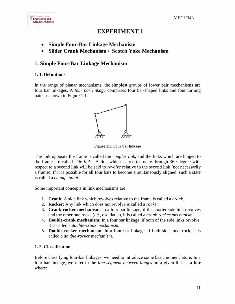
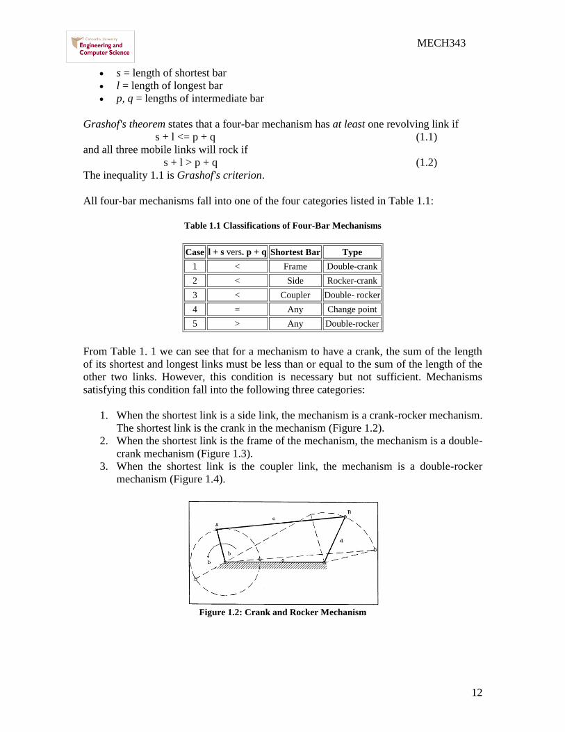
12
MECH343
s = length of shortest bar
l = length of longest bar
p q = lengths of intermediate bar
Grashofs theorem states that a four-bar mechanism has at least one revolving link if
s + l lt= p + q (11)
and all three mobile links will rock if
s + l gt p + q (12)
The inequality 11 is Grashofs criterion
All four-bar mechanisms fall into one of the four categories listed in Table 11
Table 11 Classifications of Four-Bar Mechanisms
Case l + s vers p + q Shortest Bar Type
1 lt Frame Double-crank
2 lt Side Rocker-crank
3 lt Coupler Double- rocker
4 = Any Change point
5 gt Any Double-rocker
From Table 1 1 we can see that for a mechanism to have a crank the sum of the length
of its shortest and longest links must be less than or equal to the sum of the length of the
other two links However this condition is necessary but not sufficient Mechanisms
satisfying this condition fall into the following three categories
1 When the shortest link is a side link the mechanism is a crank-rocker mechanism
The shortest link is the crank in the mechanism (Figure 12)
2 When the shortest link is the frame of the mechanism the mechanism is a double-
crank mechanism (Figure 13)
3 When the shortest link is the coupler link the mechanism is a double-rocker
mechanism (Figure 14)
Figure 12 Crank and Rocker Mechanism
13
MECH343
Figure 13 Drag Link Mechanism
Figure 14 Double Rocker Mechanism
1 3 Transmission Angle
In Figure 15 if AB is the input link the force applied to the output link CD is
transmitted through the coupler link BC (That is pushing on the link CD imposes a force
on the link
Figure 15 Transmission angle
14
MECH343
AB which is transmitted through the link BC) The angle between link BC and DC is
called transmission angle β as shown in Figure 15 For sufficiently slow motions
(negligible inertia forces) the force in the coupler link is pure tension or compression
(negligible bending action) and is directed along BC For a given force in the coupler
link the torque transmitted to the output bar (about point D) is maximum when the
transmission angle approaches to π 2
When the transmission angle deviates significantly from 2 the torque on the output
bar decreases and may not be sufficient to overcome the friction in the system For this
reason the deviation angle 2 should not be too great In practice there is no
definite upper limit for α because the existence of the inertia forces may eliminate the
undesirable force relationship that is present under static conditions Nevertheless the
following criterion can be followed
oo 5090
minmax (13)
1 4 Dead Point
When a side link such as AB in Fig 6 becomes aligned with the coupler link BC it can
only be compressed or extended by the coupler In this configuration a torque applied to
the link on the other side CD cannot induce rotation in link AB This link is therefore
said to be at a dead point (sometimes called a toggle point) In order to pass the dead
points a flywheel is usually connected to the input shaft particularly
Figure 1 6 Dead point
In Figure 16 if AB is a crank it can become aligned with BC in full extension along the
line AB1C1 or in flexion with AB2 folded over B2C2 We denote the angle ADC by and
the angle DAB by We use the subscript 1 to denote the extended state and 2 to denote
the flexed state of links AB and BC In the extended state link CD cannot rotate
clockwise without stretching or compressing the theoretically rigid line AC1 Therefore
link CD cannot move into the forbidden zone below C1D and must be at one of its
two extreme positions in other words link CD is at an extreme A second extreme of link
CD occurs with 1
Note that the extreme positions of a side link occur simultaneously with the dead points
of the opposite link
15
MECH343
1 5 Objective and Fundamentals
The experiment is designed to give a better understanding of the performance of
the four-bar linkages in its different conditions according to its geometry
Measuring the Dead point angles φ and transmission angles β at two positions
when the constant bar a at two different positions 4˝ and 6˝
1 6 Description of the Experiment
The experimental setup consists of two four-bar linkage mechanism trains as shown in
Figure 17 Careful examination of the setup should result in the correct categorization of
the linkages There is an arm following the coupler curve trace a software generated
linkage similar to the actual linkage is studied using the Working Model simulation
package
1 7 Experimental Procedure
1 Set the fixed bar a at 4˝
2 Observe the movement of the four bar linkage mechanism
3 Find the first dead point then measure Dead point angle φ and transmission angle β
4 Repeat step 3 for the second dead point
5 Set the fixed bar a at 6˝
6 Repeat the steps 2 3 4
7 Fill table (1)
Table (1)
Ground Length
(in)
Transmission Angle (β) Angle at Dead points (φ)
β1 β2 φ 1 φ 2
4
6
Figure 17 Four bar linkage Mechanism
16
MECH343
2 The Slider-Crank and Scotch- Yoke Mechanism
21 Theory
The Slider-crank (Figure 18) and the Scotch-yoke mechanism (Figure 19) setup is a
single setup which can be adapted to function as one or the other as shown in Figure 19
Figure 18 Slider crank Mechanism
Figure 19 Scotch- Yoke Mechanism
The only difference is in link 3 which is replaceable depending on the type of mechanism
required It is important to study the Kinematic and dynamic response of the mechanism
because of practical applications It is also useful in determining the Kinematic
equivalents of other mechanisms While the motion of a Scotch-yoke mechanism is
purely sinusoidal that of the Slider-crank mechanism is not The derivation of the
equations used for describing the Kinematic motions (displacement velocity and
acceleration) of a simple Slider-crank mechanism can be seen on most mechanism text
books The final equation describing the displacement may be written as
]sin1cos[
21
2
2
2
L
RLRLRX (14)
the velocity and acceleration can also be described by
21
21222 sin2
2sinsin
RL
RRV (15)
23
)sin(
)2(sin
4
1
sin
2coscos
sin2
2sinsin
222
23
222
2
222
RL
R
RL
RR
RL
RRa
(16)
X R
17
MECH343
Similarly the motion analysis for the Scotch mechanism can be found in most
mechanisms text books For this case the displacement is given by
)cos1( RX (17)
and velocity and acceleration can be written as
sinRX (18)
sincos2 RRX (19)
2 2 Objective
Obtaining the position velocity acceleration for the Slider Crank and the Scotch
Yoke mechanisms
2 3 Experimental procedure
1 Set the slider crank at 0mm for the connecting rod and 0deg for the rotating disk
2 Measure L the length of the connecting rod and R the radius for the rotating disk
3 Change the angle for the disk by 30deg each time until 360deg and each time measure
X
4 Fill the result in table (2)
5 Plot graphs between the angular displacement and the displacement X velocity V
and the acceleration a
6 Repeat for the Scotch Yoke and fill the results in table (3)
Table (2) Slider crank
Angular
Displacement
(θ)
Experimental
position X
(mm)
Theoretical
position X
(mm)
Velocity V
(mm sec)
Acceleration a
(mmsec2)
0 30 60 90
120 150 180 210 240 270 300 330 360
18
MECH343
Table (3) Scotch Yoke
2 4 Results
1 Show the difference of the results obtained in step 2 for Slider-Crank and Yoke
Mechanisms
2 Show the maximum value of velocity and acceleration given the equations
describing the velocity and acceleration for both Slider-crank and Scotch-yoke
mechanisms
3 At what angular positions the maximum value of velocity and acceleration happen
in both mechanisms
4 Plot experimental and theoretical result for displacement versus angular
displacement in the same graph as well as theoretical velocity and acceleration
versus angular displacement for both Slider-Crank and Scotch-Yoke mechanisms
Angular
Displacement
(θ)
Experimental
position X
(mm)
Theoretical
position
X( mm)
Velocity V
(mm sec)
Acceleration a
(mmsec2)
0
30
60
90
120
150
180
210
240
270
300
330
360
19
MECH343
EXPERIMENT 2
Kinematic Analysis of Norton-Type Gearbox
1 General
Norton-type gear drives are used in feed systems of machine tools to provide sufficient
speeds in a geometric progression Figure 21 shows a schematic of the drive
Figure 21 Norton-Type Gearbox used in Lathes
It consists basically of a set of gears (a) of equal diametral pitch with decreasing tooth
number arranged in a conical pattern as shown in Figure 21 A single mating gear (b) on
a sliding arm provides a means of selecting the required speed ratio The input motion is
always given to the sliding gear (b) while the output motion is taken from the conical
gear set (a)
2 Theory
The gear ratio (GR) in a gear train as shown in Figure 22 is defined as
velocityangularinput
velocityangularouputGR
Figure 22 Compound Gear Train Input Output
Reverse
a c
b
20
MECH343
The gear ratio between any two successive engaged gears is inversely proportional to the
teeth numbers n ie
2
1
1
2
n
n
W
W (21)
The procedure to find the GR is to start with the input and to calculate how the angular
velocity propagates through each successive intermeshing pair of gears based upon the
number of teeth Consider a compound gear train shown in Figure 23
Figure 23 Compound Gear Train
Suppose that the input gear speed (rotation rate) is 1600 rpm clockwise ie
rpmW 16001 (+ is clockwise) (22)
Using Equation (21)
rpmWn
nW 9601600
50
301
2
12
rpmWW 96023 (23)
where the negative sign represents for counter-clockwise direction Similarly
4
3
3
4
n
n
W
W
rpmWn
nW 480960
40
203
4
34
rpmWW 48045 (24)
and
6
5
5
6
n
n
W
W
rpmWn
nW 240480
36
185
6
56 (25)
21
MECH343
The final gear ratio GR can thus be obtained
1501600
240
velocityangularinput
velocityangularouputGR (26)
3 Objectives and Fundamentals
The experiment is designed to give a better understanding of the geometry of gear trains
and their Kinematic analysis
Measure the output velocity for the shaft and calculate the gear train
The schematic of Gear drive is shown in Figure 24 The construction of speed diagrams
of gear drives is also illustrated in Figure 25
4 General Data for Norton 36-Speed Gearbox
Motor speed 1725 rpm
Motor reduction unit ratio 60 1
Speed input to gearbox 292 rpm
Gearbox output speed range 23 -344 rpm (Fig 4)
Input torque to reduction unit 277 in lb
Output torque range 3510 -235 in lb
Figure 24 Schematic of Gear Drive
5 Experimental Procedure
1) Considering speed input to the gearbox from the motor is 292 rpm which goes to
the input shaft A
2) Observe Figure 2-5 and match the gear numbers and shaft
3) Measure the output seed for the shaft
4) Fill table (21) the experimental values
A
22
MECH343
Table 2 1 Output results
Figure 25 Speed Diagram
6 Experimental Result
1) Calculate the theoretical output speed and show the calculation
2) Calculate the gear ratio for all cases
3) Plot speed diagram for the all cases depending on the one shown in Figure 2-5
Case
Input
Output (rpm)
G-10 G-14 G-16 G-18
1
1-3
3-6
Theoretical
GR
Experimental
GR
2
2-5
3-6
Theoretical
GR
Experimental
GR
3
2-5
4-7
Theoretical
GR
Experimental
GR
23
MECH343
EXPERIMENT 3
Hook (Cardan) Joint or Universal Joint
1 Introduction
The simplest means of transferring motion between non axial shafts is by means of one or
two universal joints also known as Cardan joints in Europe and Hookrsquos joints in Britain
The shafts are not parallel to one another and they may be free to move relative to one
another For this reason this very simple spherical mechanism appears in an enormous
variety of applications The most common application is Cardan joint used in the trucks
as shown in Figure 31 A universal joint is a simple spherical four-bar mechanism that
transfers rotary motion between two shafts whose axes pass through the concurrency
points The joint itself consists of two revolute joints whose axes are orthogonal to one
another They are often configured in a cross-shape member as shown in Figure 32
2 Objective of Universal Joint
Coupling is used to connect two intersecting shafts
Consists of 2 yokes and a cross-link
Figure 31 Cardan Joint used in Trucks
Figure 32 Schematic of Cardan Joint
The transmission behavior of this joint is described by Equation (31)
12 tan
cos
1arctan
(31)
where is the momentary rotation angle of the driven shaft 2
24
MECH343
Figure 33 Schematic of Cardan Joint
The angular velocity ratio can be described by
22
2
4
sinsin1
cos
(32)
where β is the angular misalignment of the shafts and Ө is the angle of the driving shaft
It is noted that
max2
4
at oo 27090
min2
4
at ooo 3601800 (33)
if β = 0 2
4
= 1 = constant at any Ө
2
4
will vary between a minimum and a maximum during each revolution
ω2 = ω4 only at 4 instants as shown in Figure 34
This is a very big disadvantage in case of automotive vehicles this means that rear
wheels will rotate at variable speed
Figure 34 Relation between
2
4
and Ө
ω2 is constant (because engine and flywheel) speed of car cannot be variable each
revolution because its inertia and so this means tires will slip and severe wear will
happen
25
MECH343
The effect of the angle β can be shown by plotting 2
4
for different values of β (Figure
35)
Figure 35 Relation between
2
4
and β
The acceleration expression of the follower of universal joint for constant ω2 is given by
222
22
24
sinsin1
2sinsincos
(34)
Recall y = u(x)v(x) therefore yrsquo= [vursquo-uvrsquo]v2
For acceleration or retardation
-acceleration when 2Ө lies between 0 -180o
-deceleration when 2Ө lies between 180 -360o
Maximum acceleration occurs when dα4 dӨ = 0 Thus
42
2
maxsin2
sin22cos
forgives
(35)
It is possible to connect 2 shafts by 2 Hooks couplings and an intermediate shaft that the
uneven velocity ratio of the first coupling will be cancelled out by the second Condition
(Figure 36)
42 (36)
Yoke 32 lies in plane containing shaft 2 3
Yoke 34 lies in plane containing shaft 3 4
Figure 36 Two shafts by two Hooks couplings and an intermediate shaft
26
MECH343
2 Objective
Testing the affect of changing of the angle between the shaft and universal joint on the
input and output shaft speed and calculate the speed ration between output and input shaft
speed
3 Experimental Procedure
1) Fixing the input shaft angle 2 0o
2) Setting the output shaft angle 154
3) Filter setting cutoff freq 4 Scope setting ch1 500mv ch2 500mv M 50ms run
scope turn on motor After stable fluctuate signal appear on screen stop scope then
turn off motor
4) Check the input and output shaft speed by using Cursor paired We assume that at
0 N4 is min setting paired cursor at this point as t=0 ms Moving cursor along
ch2 signal and record t and N4 by ∆ __ms __v Fill table 3-1 N2 is input shaft
speed It is constant
5) Repeat step 2 setting the output shaft angle 304 Fill table 3-2
6) Plot the graph of velocity ratio during one cycle for both cases Compare with
theoretical plot using equation 32
Table 3 1 Test results of Cardan joint
154
Table 3 2 Test results of Cardan joint 304
(o) 0 45 90 135 180 225 270 315 360
t (ms)
N4(v)
N2(v)
N4N2
(o) 0 45 90 135 180 225 270 315 360
t (ms)
N4(v)
N2(v)
N4N2
27
MECH343
EXPERIMENT 4
Mechanical Oscillator for Measurement of Friction Coefficient
1 Introduction
The mechanical oscillator is an apparatus which allows the experimental
determination of friction coefficient by measuring the period of an oscillating table As
shown in Figure 41 the apparatus consists of two counter rotating wheels upon which is
placed a table of uniform weight
Figure 41 The mechanical oscillator
If the center of gravity of the table is not centered when it is placed on the rotating wheels
then more of its weight will rest upon one wheel than upon the other Consequently the
frictional forces will not be equal and the table will move in the direction of the larger of
the two forces But the inertia of the table will carry it too far past the center point and the
other wheel will exert the larger frictional force Thus the table will oscillate back and
forth at a frequency which depends upon the coefficient of friction
The basic step to find the equation of motion of the system is to construct the Free Body
Diagram of the oscillating table Figures 2(a) 2(b) and 2(c) show this procedure
Summing the forces in the horizontal plane we have
0RRXg
W21 (41)
or
0XL
W2X
g
W
(42)
hence
0XL
g2X
(43)
28
MECH343
Figure 42 procedure of finding the equation of motion
Since the differential equation of motion of free vibration for a one degree of freedom
system is of the form
02 XX n (44)
where n is the natural frequency of the system then
L
g22
n
(45)
But L
gfn
24 222 (46)
where
f = the frequency of the oscillating table in cps
L = the distances between wheel centers in ft
g = gravity constant
hence 2
22f
g
L (47)
The solution of the equation of motion can be written in the form
tBtAX nn cossin (48)
With the initial condition
00 XandXXt O (49)
one gets oXBandA 0 (410)
The response of the oscillating table is therefore
tL
gXX o
212
cos
(411)
29
MECH343
tL
g
L
gXX o
21212
sin2
(412)
tL
g
L
gXX o
212
cos2
(413)
Thus it may be concluded that the response of the oscillating table is governed by the
initial displacement X0 the coefficient of friction micro and the difference between wheel
centers L
2 Objectives
The experiment is designed to illustrate some of the direct applications of the
theory of vibration to the measurement of physical quantities The experiment also
demonstrates the differences between mathematical models and actual physical systems
Calculate the friction coefficient between the wheels and the bars
3 Description of Experiment
The oscillating table apparatus consists of four grooved wheels mounted on two
axels which are driven by a 120 HP electric motor and a gear reduction unit in opposite
directions The table consists of circular rods connected in a rectangular shape such that
the rods are guided by the grooved wheels
4 Experimental Procedure
1) Measure L the length between the centers of the two wheels
2) Locate one of the bars on the wheels
3) Select two different speeds for the wheels and when it starts rotating and the bar
moving calculate the time for 10 oscillations
4) Calculate the experimental coefficient of friction μ through the following
equation 2
22f
g
L When f is the frequency g gravity acceleration L the
length between the centers of the two wheels Fill table 4-1
5) Find the theoretical coefficient of friction μ for all bars
6) Compare between theoretical and experimental coefficient of frictions μ
Table 4 1 Combinations for measuring the friction coefficient
Case Material of
the bar
Speed
(rpm)
Time taken
for 10
oscillation
Frequency
(f)
Coefficient
of friction
(micro)
Standard
coefficient
of friction
1 Steel
2 Brass
3 Aluminum
30
MECH343
EXPERIMENT 5
5-1 PLANETARY GEAR TRAIN KINEMATICS
1 Introduction
A planetary gear train is one in which the axis of some of the gears may have motion A
planetary gear set always includes a sun gear one or more planet gears and a planet
carrier or arm which sometimes called as sun-and-planet planetary gear train as shown in
Figure1
Figure 51 Planetary gear train
A planetary gear set as shown in Figure 52 is one having two degrees of freedom This
means that the motion of each and every element of the mechanism is not defined unless
the motion of two of its elements is specified To make the planetary set a one degree of
freedom gear train one must fix the motion of one element of the mechanism
Figure 52 Sun-and-planet planetary gear train
2 Solution of Planetary Trains by Formula Methods
Figure 53 shows a planetary gear set which is composed of a sun gear 2 an arm 3 and
planet gears 4 and 5
31
MECH343
Figure 53 Compound Planetary Gear Set
We can express the velocity of gear 2 relative to the arm 3 in the form
3223 nnn (51)
3553 nnn (52)
Dividing Equation (52) by (51) gives
32
35
23
53
nn
nn
n
n
(53)
Since this ratio is the same and is proportional to the tooth numbers it is equivalent
therefore to the train value e
32
35
nn
nne
(54)
Or AF
AL
nn
nne
(55)
where nF = rpm of first gear in train
nL = rpm of last gear in train
nA = rpm of arm
The experiment is designed to demonstrate the fundamentals of planetary gear train and
to show all possible motions that can be obtained with this type of gear trains
3 Objective
Calculate the gear train ratio for the planetary gearbox and the degrees of
freedom that the system has
4 Experimental Procedure
For the planetary gear trains mechanism shown in Figure 51
1) Calculate the degree of freedom to the planetary gear system
2) Calculate the gear train ration through the following equation
21
23
nn
nne
When the outer ring is fixed
When the planet gears are fixed
32
MECH343
5-2 The Borg-Warner Model 35 Automatic Transmission
Simulator
1 Introduction
The Borg-Warner Model 35 Automatic Transmission comprises a three element
torque converter--coupling and a planetary gear set to provide three forward ratios and
reverse
The planetary gear set consists of two sun gears two sets of pinions a pinion
carrier and a ring gear
Power enters the gear set via the sun gears In all forward ratios power enters
through the forward sun gear In reverse it enters through the reverse sun gear Power
leaves the gear set by the ring gear and the pinions are used to transmit power from the
sun gears to the ring gear
In reverse a single set of pinions is used which causes the ring gear to rotate in the
opposite direction from the sun gear In forward ratios a double set of pinions is used to
cause the ring gear to rotate in the same direction as the sun gear
The Carrier locates the pinions relative to the two sun gears and the ring gear also
forming a reaction member for certain conditions The various mechanical ratios of the
gear ser are obtained by the engagement of hydraulically operated multi-disc clutches and
brake bands
Power flow in each ratio is achieved by locking various elements of the planetary gear set
as follows
1st Gear (Lockup selected)
The front clutch is applied connecting the converter turbine to the forward sun
gear The rear band is also applied holding the pinion carrier stationary The gear set
provides the reduction of 239 l The reverse sun gear rotates freely in the opposite
direction to the forward sun gear
33
MECH343
1st Gear (Drive selected)
The front clutch is applied connecting the converter turbine to the forward sun
gear The one-way clutch is in operation preventing the pinion carrier from moving
opposite to the engine rotation The gear set again provides the reduction of 239 1 On
the overrun the one-way clutch unlocks and the gear set freewheels
2nd Gear (Lockup or drive selected)
Again the front clutch is applied connecting the converter turbine to the forward
sun gear The front band is applied holding the reverse sun gear stationary The pinions
now walk around the stationary sun gear and the gear set provides the reduction of 145
l
3rd Gear (Drive selected)
Again the front clutch is applied connecting the converter turbine to the forward
sun gear The rear clutch is applied connecting the turbine also to the reverse sun gear
Thus both sun gears are locked together and the gear set rotates as a unit providing a
ratio of 1 1
Neutral and Park
The front and rear clutches are released and no power is transmitted from the
converter to the gear set
Reverse
The rear clutch is applied connecting the converter turbine to the reverse sun gear
The rear band is applied holding the pinion carrier stationary providing a reduction of
209 l
2 Gear Ratios
119866119890119886119903 119877119886119905119894119900 120579119900120579119894
=1
239
The carrier is held stationary to provide the
reaction member and the gears operate as a
Simple gear train
34
MECH343
The reverse sun gear is held to that the gears
now operate as an epicyclic gear train
For an epicyclic gear train shown as following
119866119890119886119903 119877119886119905119894119900 120579119900120579119894
=1
145
119894134 =
1205961 minus 1205964
1205963 minus 1205964= minus
11988521198851
11988531198852prime
119900119903 120596119871
32
67= 120596119869 minus 120596119871 120596119869 =
99
67120596119871
For our transmission show as above
119894119865119869119871 =
120596119865minus120596119871
120596119869minus120596119871= minus
119885119866
119885119865
119885119867
119885119866
119885119869
119885119867=
67
28 (1)
119894119865119870119871 =
120596119865minus120596119871
120596119870minus120596119871= minus
119885119866
119885119865
119885119867
119885119866
119885119870
119885119867= minus
32
28 (2)
Hence minus120596119871
120596119869minus120596119871= minus
67
68
28
32
From (2) 120596119865 minus 120596119871 =32
28 120596119871 120596119865 =
60
28120596119871
Therefore 119894119865119869 =120596119865
120596119869=
60
28
67
99= 145021645
So 120579119900
120579119894=
1
145
35
MECH343
119866119890119886119903 119877119886119905119894119900 120579119900120579119894
=1
1
Both sun gears are locked together and the
gears set rotates as a unit
119866119890119886119903 119877119886119905119894119900 120579119900120579119894
=1
209
With the reverse gear engaged power is
applied to the reverse sun gear The planet
carrier is held stationary so that the planet
gears rotate the ring gear in the opposite
direction to the reverse sun gear
36
MECH343
3 Experimental Procedure
Pins and slotted plates represent the multi-disc clutches and brake bands The various
gear ratios of the gear set may be obtained by inserting the appropriate pins as indicated
below
A B C D E F
Lockup 1Drive 1
Lockup 2Drive 2
Drive 3
Reverse
Neutral
Park Note
1 Lose all pin and turn input shaft and output shaft make sure input shaft disk and
output shaft disk indicate to 0 then lock pins for each case
2 Turn input shaft one turn (360 ) read output disk (degree)
3 Fill out following table
Input (degree) Output (degree)
Lockup 1Drive 1 360
Lockup 2Drive 2 360
Drive 3 360
Reverse 360
4 Results
According to power flow and gear ratio figures for each case referring to 2nd gear
ratio calculation derive and calculate gear ratios for 1st 3
rd and reverse shift Compare
them with your experimental results
37
MECH343
EXPERIMENT 6
Static and Dynamic Balancing
1 Objective
The objectives of this experiment are
Understanding the concept of static and dynamic balancing
Understanding unbalance torque
Justifying theoretical calculation for balancing with experiment
Balancing the shaft by the four given masses
2 Introduction
Unbalanced dynamic forces effects have profound influence on the working and
of rotating machinery like turbines compressors pumps motors etc These forces act
directly on the bearings supporting the rotor and thus increase the loads and accelerate the
fatigue failure These unbalanced forces induce further mechanical vibrations in the
machinery and connected parts thereby creating environmental noise problem through
radiation of sound Hence it is desirable to balance all such uncompensated masses and
thus reduce the effect of unbalance forces in a dynamics balancing machine
Balancing is the technique of correcting or eliminating unwanted inertia forces which
cause vibrations which at high speeds may reach a dangerous level An important
requirement of all rotating machinery parts is that the rotation axis coincides with one of
the principal axis of inertia of the body After a roll is manufactured it must be balanced
to satisfy this requirement especially for high speed machines The condition of
unbalance of a rotating body may be classified as static or dynamic unbalance
2 1 Static Unbalance
An idler roll is statically balanced if the roll doesnt rotate to a heavy side when free to
turn on its bearings Thus the rolls center of gravity is on the axis of rotation Static
unbalance (Figure 61) creates a centrifugal force when rotating which causes deflection
of the roll Idler rolls are sometimes static
balanced only when the roll operates at slow
speeds
The static unbalance usually happens because
of errors in the manufacturing tolerances of
the rotating parts Therefore static imbalance
is essentially a weighing process in which the
part is acted upon by either gravitational or
centrifugal force This type of unbalance
could be easily reduced or removed by static
balancing
Figure 61 Static (or force) Unbalance
38
MECH343
2 2 Dynamic Unbalance
An idler roll may be in perfect static balance and not be in a balanced state when rotating
at high speeds A dynamic unbalance is a ldquocouplerdquo or twisting force in two separate
planes 180 degrees opposite each other (Figure 62) Because these forces are in
separate planes they cause a rocking motion from end to end A roll that is unbalanced
will cause 1) machinery vibrations 2) web
flutter and 3) a decrease in bearing life due to
unnecessary forces
To dynamically balance a roll it must first be
statically balanced Then the roll must be
rotated to its operating speed and have the
dynamic unbalance eliminated by adding or
subtracting weight The determination of the
magnitude and angular position of the
unbalance is the task of the balancing
machine and its operator Balancing
machines are provided with elastically
supported bearings in which the idler roll may
spin Because of the unbalance the bearings
will oscillate laterally and the amplitude and
phase of the roll are indicated by electrical
pickups and a strobe light
Figure 63 shows a long rotor which is to be mounted in bearing A and B We might
suppose that two equal masses m1 and m2 are placed at opposite ends of the rotor and at
equal distances r1 and r2 from the axis of rotation Since masses are equal on opposite
sides of the rotational axis the rotor is statically balanced in all angular positions But if
the rotor is caused to rotate at an angular velocity ω radsec the centrifugal forces m1r1ω2
and m2r2ω2 act respectively at m1 and m2 on the rotor ends These centrifugal forces
produce the equal but opposite bearing reactions FA and FB and the entire system of
forces rotate with the rotor at the angular velocity ω Thus the rotor is to be statically
balanced and at the same time dynamically unbalanced
Figure 63 Dynamically Unbalanced Rotor
Figure 62 Dynamic (or couple) Unbalance
39
MECH343
3 Principle and Theory of Operation
Consider a body of mass M rotating with a uniform angular velocity about O with
eccentricity e as shown in Figure 64 The centrifugal force Fc acting on the axis of
rotation is Me2 This force is therefore very sensitive to speed and hence there is a need
to reduce this force either by operating at lower speeds or by decreasing the eccentricity
as shown in Figure 65
O
e
M
M e
2
Figure 64 Unbalanced Disc
Center of rotation
( new center of
gravity )
Rotating Disc Added mass m
Center of gravityOriginal center
of gravity
(a) (b)
Figure 65 Illustration of The Simplest Method of Static Balancing
In general it is desirable to make e as low as possible If the rotor thickness to diameter
ratio is less than 05 and speed are below 1000 rpm the rotor can be single plane
balanced - otherwise two-plane balancing is necessary In the single plane balancing
technique with a rotor of mass mi and radius ri from the axis of rotation and lying in the
same plane the condition for static balance is used
0~iirm (61)
where i = 1 2 which denotes the total number of masses and m denotes the mass The
vector ir~ represents the eccentricity e of the mass mi from the axis of rotation
When the bodies are rotating in several planes the condition for dynamic balance has to
be satisfied in addition to that for static balance This is given by
0~~ iii rzm (62)
where iz~ is the axial coordinate vector of the mass mi measured for a chosen datum In
the two-plane balancing technique instead of satisfying Equations (61) and (62)
40
MECH343
explicitly Equation (62) is used with two different datum planes for iz~ Mathematically
if the distance between these two plane is oz~ then
0~)~~( ioii rzzm (63)
It is therefore clear that Equations (62) and (63) imply the satisfaction of Equation
(61) Conceptually it means that if a system of bodies rotating in several planes is in
dynamic balance with respect to two different datum planes then the system is also in
static balance This is the principle of the two-plane balancing technique
4 Description of Experimental Apparatus
Figure 66 shows the Static and Dynamic Balancing Apparatus It consists of a perfectly
balanced shaft with four rectangular blocks clamped to it The shaft is mounted in ball
bearings and it is driven by a 12 volt electric motor through a belt and pulley drive The
shaft assembly is mounted on a metal plate resting on four resilient rubber supports
which allow the mount to vibrate when the shaft is not balanced
The rectangular blocks can be clamped to the shaft at desired out-of-balance moments by
means of discs having eccentric holes of various diameters The discs are fixed to the
blocks by hexagon socket set screws Any longitudinal and angular position of a block
relative to the shaft can be set by linear and protractor scales provided Adjacent to the
linear scale is a slider which can be pushed against the block to read its longitudinal
position The slider also serves as a datum stop against which the blocks can be held
when reading their angular position on the shaft
The out-of-balance moments are measured by fitting the extension shaft and pulley to the
main shaft Each rectangular block is then clamped to the shaft in succession A cord with
a weight bucket at each end is hung on the pulley and bearing balls are placed in the
bucket until the block has turned through 90deg The out-of-balance moment is proportional
to the number of balls required
to turn the block
A Perspex dome serves as the
safety cover The shaft cannot
be driven unless the dome is in
position which is achieved by
micro switches actuated by the
dome The motor switch on the
front panel is spring loaded so
that the motor cannot be left
running The motor requires a
power supply of 12 volts at 2
amperes which is provided by
E66E90 speed controller
Figure 66 Static and Dynamic Balancing Apparatus
41
MECH343
5 Experimental Procedure
5 1 TEST 1 Static Balancing
1 Looking at the shaft from the side the masses will be as shown in figure 6-7
each mass has an angle θ with horizontal
Figure 6-7 Shaft view from the side
2 The masses forces are given by the following table 6-1
The masses values Table 6-1
3 In order to balance the shaft statically the sum of the forces will be equal zero
as the following equations
sum F=0
F1cos θ1+ F2cos θ2+ F3cos θ3+ F4cos θ4=0 (1)
F1sin θ1+ F2 sin θ2+ F3 sin θ3+ F4 sin θ4=0 (2)
4 Since we have just two equations with four unknown angles we assume
θ1=0ordm θ2=90ordm
5 Solving the two equations or using force polygon by AutoCAD to find the θ3
θ4
5 2 TEST 2 Dynamic balancing
1 Looking for the shaft from in front the masses create the forces as shown in
figure 6-8 each mass has an arm X create a momentum
F1
F2
F3
F4
42
MECH343
2 In order to balance the shaft dynamically the sum of the momentum will be
equal zero as the following equations
sum M=0
F1cos θ1X1+ F2cos θ2X2+ F3cos θ3X3+ F4cos θ4X4=0 (1)
F1sin θ1X1+ F2 sin θ2X2+ F3 sin θ3X3+ F4 sin θ4X4=0 (2)
3 Since we have just two equations with four unknown arms we assume
X1=50 mm X2=100 mm
4 Solving the two equations or using momentum polygon by AutoCAD to find
the X3 X 4
TABLE 6 2
Block 1 2 3 4
Mass 88 82 74 64
Angle θ(ordm) 0 90
Arm X (mm) 50 100
6 Typical Calculations
The basic equations that are used for balancing purposes are
0rW ii (63)
0rWa iii (64)
Suppose that block (1) is placed 17 mm from the left end of the shaft at zero angular displacement and that
block (2) is placed 100 mm from it at 120deg The measured out-of-balance moments are as follows
Figure 68 In front shaft view
43
MECH343
TABLE 6 3 OUT-OF-BALANCE MOMENTS
It is first necessary to draw the moment polygon of Wr values as shown in Figure 68 to determine the
angular positions of blocks (3) and (4) W1r1 and W2r2 are known in both magnitude and direction The
vector W1r1 has been drawn at positive X-direction (θ = 0) The lengths of vectors W3r3 and W4r4 are known
and arcs can be drawn from the ends of W1r1 and W2r2 to get the directions of the unknown vectors
Figure 69 shows the diagram of the angular positions and the corresponding longitudinal locations of the
blocks on the shaft are 17 mm for the first 117 mm for the second block
To find the longitudinal positions of the other two blocks we designate distance of block (3) by a3 and
distance of block (4) by a4 measured from block (1) so block (1) is the reference and will not appear in
calculations
Draw a vector a2W2r2 = 100 (82) units long parallel to r2 and vectors a3W3r3 and a4W4r4 parallel to r3 and r4
respectively so that the moment polygon is closed The lengths of vectors a3W3r3 and a4W4r4 can be
measured and the magnitudes found by using the scale factor From these a3 and a4 can be calculated
Notice that the sense of vector a3W3r3 is reverse In order to maintain vector a3W3r3 the only possible
solution is to reverse a3 So from the vector polygon (triangle) it follows
a3 = -12 mm
a4 = 124 mm
This means that block (3) should be located 5 mm from the left end of the shaft The blocks should be
positioned as follows
Block Angular Position (Deg) Longitudinal Position (mm)
(1) 0 17
(2) 120 117
(3) 190 5
(4) 294 141
The values of a3 and a4 can be found analytically using complex vector approach
Real and imaginary components yield
100(82) cos 120deg + (74) a3 cos 190deg + (64) a4 cos 294deg = 0
100(82) sin 120deg + (74) a3 sin 190deg + (64) a4 sin 294 deg = 0
which reduce to
4100- 7288 a3 -2603 a4 = 0
71014- 1285a3 -5847 a4 = 0
44
MECH343
Solving the two equations gives a3 = -1194mm a4 = 12396mm
The values compare very well with those obtained graphically
In order to obtain independent results it is suggested that Wr values of the blocks are varied by using
different positions of the discs with eccentric holes The angular displacements between blocks (1) and (2)
may also be varied
Figure 69 Moment Polygon of Wr
45
MECH343
EXPERIMENT 7
Machine Fault Simulator (MFS)
1 Theory
Refer to experiment number 6
2 Description of Experimental Apparatus
Figure 71 shows the machine fault simulator The rotor is driven by a variable speed
motor via a flat belt and the rotor rotational speed is captured through a digital
tachometer The vibration due to the unbalanced rotor is measured and fed directly into
the on-board processor of the machine
Figure 71 Machine Fault Simulator
3 Objective
In this experiment we will study the reaction of the shaft and the motor when the shaft is
balanced and when it is unbalanced
4 Experimental Procedure
1) Run the Vibro-Quest Software
o Define a ldquoNew Projectrdquo (under root)
o Fill up the window select ldquoProject namerdquo click ldquoNextrdquo
o Select ldquoNonerdquo from the menu on the right side click ldquoNextrdquo
Belt
Motor
Disk A Disk B
Reciprocating
Mechanism
Speed
Control
46
MECH343
o Review the table (do not change the default) click ldquoNextrdquo
o Review the table check the setting data click ldquoNextrdquo
o Click ldquoDonerdquo
o Review the information provided if they are not ok ldquoGo backrdquo to modify
the data then click ldquoFinishrdquo
2 Select ldquoDatardquo from the toll bar on the computer
3 Name the ldquoTest Titlerdquo in the window Insert the parameters used in the test and
click ldquoNextrdquo
4 Review the information provided in the window and click ldquoNextrdquo
5 Chose 2000 as Frequency limit 1600 for Space line Leave the rest information as
defaulted and ldquoGO DAQrdquo
2) Running the Machine Fault Simulator
Select the required speed (rpm) change it to frequency (Hz) using the following
relation 60)rpm(n2)Hz(f
1 Run the machine using speed control system at desired speed
2 Wait about 15 seconds to stable the system
3 Click onrdquo START RECORDINGrdquo
4 When the recording is finished save the file under the root of ldquoDatardquo of base line
at the subdirectory that you want to compare with the other data (for example if
you are running the machine at 20 Hz save the your file under 20 Hz subdirectory)
5 Now select the ldquoProject namerdquo from the left menu all the relevant tests will
appear at the right table under the ldquoTest Explorerrdquo
6 To compare the data from different files Hold down the ldquoShiftrdquo key and select
any two interested files that you are going to compare
7 Click on ldquoComparerdquo to observe the difference between the unbalanced system
with a base system
8 To observe more clearly the difference between the frequency responses of the
different test click on ldquoOverlayrdquo
TEST 1 Imbalance Effects on Vibration response
Install the defined weight in one of the taped hole in rotor disk A and tight it
securely with a nut
Close the cover of MFS
Change the motor speed and record vibration level at each bearing For this
purpose you don not need to define new project for each speed define a new
project( follow steps 1-6 from section 3) then follow steps 1-2 for each speed
from section 4
Measure the average level of amplitude at each speed and Plot it against the speed
Repeat steps 2-5 for 2 different weights at 2 different radius and angles
47
MECH343
TEST 2 Balancing the Imbalance Rotor
Add weight at different radius and angles using the ldquosample calculationrdquo to
balance the rotor
If the rotor is balanced define a ldquoNew projectrdquo and follow steps 3-8 of Section 4
Fill Table 7 1
TABLE 7 1
Unbalance weight on disc A ____________ angular position _______________
Mass Added on disk B gr r (mm)
Amp baseAmp New
48
MECH343
EXPERIMENT 8
DETERMINATION OF SPUR GEAR EFFICIENCY
1 Objective
The main objective of the experiment is to determine the efficiency of the
Spur gear and worm gear unit
2 Introduction and theoretical background
21 Pinion gear
Two intermeshed toothed wheels make up a pinion gear This type of gear
permits a positive transmission of motion and torque Wheel pairs are available in
different shapes and shaft configurations Figure 1 explains the various types of gears and
their arrangements
Fig8 1 Various types of gear arrangements
22 Worm gear
A worm gear is a screw-type transmission unit whose axes generally intersect at
right angles The worm and wheel make contact on a straight line Normally the worm
has a cylindrical core and the wheel globoid toothing Units with a very high performance
49
MECH343
consist of a globoid worm and globoid wheel A worm gear with a cylindrical worm has
the following special features
High load capacity compared with spur gears due to linear contact
Low-noise operation and high absorption of vibrations
Wide transmission range down to low ilt110
High efficiency at high transmission ratios high efficiencies(η le 98 ) can be
achieved with very sophisticated designs under favorable operating conditions a
decrease in pitch angle (high transmission ratio) or speed is accompanied by a
corresponding decrease in efficiency (to η le 50 )
Self-locking operation
Smaller and lighter design compared with spur bevel gear units possessing high
transmission ratios
23 Basic definitions
Drive torque
The drive torque is the product of the force F and the lever arm l on which the
force acts
M = F X l (1)
M is in Nm F is in N and l in m
Drive power
The drive power of a rotating shaft is the product of the torque M and angular
frequency ω P = M X ω (2)
and 60
2 n (3)
P is in W n is in rpm
Efficiency
The efficiency is defined as the ratio between the output and input powers It has a
maximum theoretical value of 1
in
out
P
P (4)
where speed i
nn 1
2
50
MECH343
3 Experimental set-up
Figure 2 shows the complete view of the experimental set up
Fig8 2 Complete view of GUNT AT 200 experimental set up
The modules comprising the drive unit spur gear worm gear and magnetic
powder brake are mounted on a profile frame The DC shunt motor is designed for right-
hand and left-hand rotation The drive unit is electrically powered via control housing
The control unit adjusts the DC machinersquos speed via its armature voltage Its target speed
is set by means of a potentiometer on this housing Its actual speed is measured and
indicated by means of an inductive proximity switch and evaluation unit The speed is
51
MECH343
measured inductively by a contactless sensor disc and indicated by a digital display
element on the control unit Electronic thyristor speed control with I x R compensation
provides a high torsional rigidity The reaction torque exerted on the drive housing is
measured by means of a spring force meter connected to a lever arm
The transmission units consist of a 2-stage spur gear with transmission
ratio i = 135 and a single-stage worm gear with transmission ratio i = 14The
transmission torque can be determined on the drive side as well as the brake side To
facilitate adjustment of the brake torque the brake characteristic (current torque) is
recorded in a preliminary experiment Moments are determined through power
measurements (spring balance) with a known lever arm The moments measured input
speeds and transmission ratios are used to determine power and efficiency
The magnetic powder coupling consists of two independently mounted
rotors ie a primary and a secondary rotor both furnished with ball bearings The
primary rotor also serves as a coil carrier If one of these two rotors is deactivated the
magnetic powder coupling can also be used as a brake The air gap between the two
rotors contains a special magnetic powder If a direct voltage is applied to the excitation
winding the powder aligns itself with the resulting magnetic field lines to form a
compact mass providing a frictional link between the primary and secondary rotors The
value of the torque depends on the adjusted current When the current-proportional
moment is exceeded slippage occurs without any transition
4 Experiments procedure
As shown in Figure 82 the complete view of the experimental set up for this
experiment there is input as the motor speed and the output as excitation current so that
there is two steps for this experiment
After making sure spur gear is connected as shown in Figure 83
1) Fix the output excitation current at I= 50 mA and change the speed of the motor as
shown in the table (1) each time measure the motor force F1 and the brake force F2
52
MECH343
Figure 83 Configuration of spur gear unit experimental set up
Measurement data to determine the efficiency of Spur gear unit Table (1) I = 50mA
SlNo Motor speed
( n1 ) rpm
Motor holding
force ( F1 ) N
Brake holding force
( F2 ) N
Efficiency ( η )
1 500
2 1000
3 1500
4 2000
5 2500
In order to find out the spur gear efficiency we go through the following equations
The general equation for the spur gear efficiency is
in
out
P
P
The drive power of a rotating shaft is the product of the torque M and angular
frequency ω P = M X ω
The drive torque is the product of the force F and the lever arm l on which the
force acts
M = F Arm
When the arm for the motor Arm1=25 mm and for the brake Arm2=50 mm
53
MECH343
And the angular velocity from the following equation
60
2 n
In order to find the speed for the brake we use this ratio assuming i= 135
i
nn 1
2
2) Fixing the input n1= 1500 rpm and changing the output and filling table (2)
Recorded values of the excitation current and the force on the lever arm table (2)
Speed n1= 1500 rpm
Excitation current I (mA) Force F2 on the lever arm (N)
50
70
90
110
130
150
130
110
90
70
50
5 Experiments Results
1) Plot the characteristics curve between the current I and the force on the lever arm
F2
2) Plot the characteristics curve between the current I and the torque M
3) Determine the efficiency of the spur gear unit Comment on the errors on the
efficiency if the calculated efficiency deviates from the realistic values of 80 -
90
54
MECH343
EXPERIMENT 9
ANALYSIS OF LINKAGE MECHANISM
Try to build a linkage mechanism as the figure below
Steps
1 Turn on grid line from View-workspace-grid lines as below
2 Select rectangle tool
55
MECH343
3 Click and drag a small rectangle
4 Click the rectangle copy it (CTRL+C) paste it (CTRL+V) two times
5 Change the length of each rectangle by selecting it and writing down the desired
length in the text box named W
Make the length as (3 ndash 332 - 4)
56
MECH343
6 Use the rotate tool and the select tool to arrange the rectangles
Make sure that the spacing is 4 units as shown below
7 Put a motor at the lower end of the left link
- First select the motor - Then click at the desired point
57
MECH343
8 Put a pin joint at the lower end of the right link
- First select the pin joint - Then click at the desired point
9 Put a point element at the remaining ends
- First double click (this
enable you to assign multiple
points) on the point element
It should look like below
58
MECH343
10 Join the links by selecting two points then selecting Join
Click the arrow select tool
Select first point ndash
press SHIFT and
click the other point
Press
Join
They should look like
below
11 Repeat the same for the remaining two points Your model should look like below
59
MECH343
12 Click RUN ( ) and watch it rotating
13 Now we want to capture the velocity of the joint between the left link and the middle
one
- Select it and click on Define ndash Vectors-
Velocity
Click Run and watch the velocity change
Note that by clicking on the link itself and defining the velocity the program calculates
the velocity of the CG of the link
14 Now you are ready to try different measurements
Acceleration Total Force Gravitational Force
60
MECH343
15 Select a link and use the measure tool
X- Position Graph
Y- Position Graph
61
MECH343
Measuring velocity values
16 Now try to change the length of any of the links and RUN the model and observe
for any change if any and explain
17 Change the mass of any of the links and observe for any change in velocity and
force And Why if there is any
18 Now double click on the motor (resetting the mass for any link that has been
changed) and notice that the value for velocity is 1 radsec Change this to make it the
same value for acceleration and torque Write what you observe and try to explain
19 Now increase the mass for one link (eg left one) gradual and see how this will
affect the motion for a fixed value for torque velocity or acceleration of the motor
20 Now replace the middle link with two links connected with total length as the
middle one run observe and explain
21 Based on (20) search for what is the equation relation or rule that governs the
mechanism motion
62
MECH343
EXPERIMENT 10
NUMERICAL DYNAMIC SIMULATION FLYWHEEL
Problem Definition
In the two cycle piston engine shown explosive gases are
ignited in the combustion chamber above the piston The
explosions apply a force of 150 N for the duration of every
downward stroke The engine is equipped with a speed
limiting device (rev limiter) which prevents the rotational
speed from exceeding a set value (red-line) The masses of
the piston and connecting rod are 075 kg and 15 kg
respectively The mass of the crankshaft-flywheel assembly
is 30 kg Given that the red-line of the engine is 35 radsec
(340 rpm) Assume the crankshaft-flywheel assembly can
be modeled as a circular disk
Objective
Determine the forces at the crankshaft bearing (point A) and connection rod (point B)
bearing
Solution
1 INTRODUCTION
Engines that exceed the manufacturers maximum speed (over-revving) may be subject to
excessive wear and possible failure To prevent over revving internal combustion
engines are often fitted with a device known as a rev-limiter When an engine exceeds its
red-line rev-limiters interrupt the ignition system slowing the engine down Once the
speed drops below the maximum the ignition system is switched back on In this exercise
you will model an internal combustion engine equipped with a rev-limiter The engine
has three bodies the piston the connecting rod and the crankshaft The piston will be
modeled by a square body The connecting rod will be modeled by a rectangular body
The crankshaft will be modeled as a circular body The bodies will be drawn sized and
joined to each other and the background The pistons cylinder walls will be modeled with
a keyed slot joint The force of combustion will be modeled by a force attached to the top
of the piston The resulting forces at the bearings will be measured
2 SETTING UP THE WORKSPACE
For this exercise three changes in the workspace will be made First for clarity the x-y
axes will be displayed The unit of distance will also be changed from meters (default) to
millimeters
63
MECH343
If the x-y axes are not currently displayed choose Workspace from the
View menu and choose XY Axes from the Workspace submenu The x-y
axes provide a reference frame for building a simulation
Choose Numbers and Unitshellip from the View menu The Numbers and
Units dialog appears
Click the More Choices button The dialog box expands
Click and hold in the Distance field (Figure 1) The pop-up menu appears
Choose millimeters from the Distance pop-up menu
Click in the Rotation field and choose Radians from the pop-up menu
Click OK
3 CREATING THE COMPONENTS
This exercise has three objects a 15 kg connecting rod a 075 kg piston and a 30 kg
crankshaft (see Figure 2 below) The connecting rod will be modeled by a thin rectangle
400 mm in length Its width will be thin 150 mm so it closely resembles the actual
connecting rod The crankshaft as stated in the exercise is modeled as a circular disk
with a 200 mm radius and a mass of 30 kg A 200 mm square object will represent the
piston The objects will be created sized and initialized in the following steps
Creating the Crankshaft
The crankshaft is represented by a circle with a radius of 200 mm and mass of 30 kg
These parameters will be set using the Geometry and Properties utility windows
I To draw the crankshaft
64
MECH343
bull Click the Circle tool in the Toolbar
bull Click once on the background Move the mouse to expand the circle and click
again to complete sketching
II To set the mass of the crankshaft
Choose Properties from the Window menu
Click the mass field and enter the value 30
III To set the size of the crankshaft
Select the crankshaft if it not already selected
Click the Radius field (labeled ldquorrdquo) of the Coordinates bar and enter the value 200
(Figure 3)
IV Zooming In
The circle will appear small after sizing To make the rectangle easier to manipulate and
appear larger the workspace will be magnified using the Zoom tool To zoom in
Click the Zoom In tool in the Toolbar
Click near the circle The objects in the window are magnified by a factor of two with
each click of the mouse To zoom out while the Zoom In tool is selected hold down
65
MECH343
the Shift key (the magnifying glass pointer changes to ldquo-rdquo) and click Your screen
should be similar to Figure 4 below
Figure 4 The workspace after zooming in
Click the Arrow tool in the Toolbar or press the spacebar to deselect the Zoom In
tool
Creating the Piston
For this exercise the piston will be modeled as a 200 mm square with the mass of 75 kg
The Square tool will be used to draw the piston and the Properties window will be used
to set its mass
I To draw the piston
Choose the Square tool in the Toolbar On systems the Square tool is ldquohiddenrdquo in the
RectangleSquare pop-up palette by default Click and hold on the Rectangle tool to
bring the pop-up palette in view (Figure 5 below)
Click once on the background drag to the right and click again to complete
sketching A square appears on the screen To set the size of the piston
Click in the Height or Width field of the Coordinates bar and enter 200 Either field
changes both the height and the width of the object so that it remains square
Figure 5 RectangleSquare pop-up palette
II To set the pistonrsquos mass
bull Select the piston if it not already selected
bull Choose Properties from the Window menu
66
MECH343
bull Click in the mass field and enter the value 075
Creating the Connecting Rod
In this exercise the connecting rod is represented by a rectangle drawn with the
Rectangle tool and sized using the Geometry window To approximate an actual
connecting rod the rectangle will be given a mass of 2 kg a height of 500 mm and a
width of 100 mm
To draw the connecting rod
I Choose the Rectangle tool in the Toolbar (On systems the Square tool used above
may have replaced the Rectangle tool in the Toolbar If so the Rectangle tool may be
selected from the hidden pop-up palette by clicking and holding on the Square tool in
the Toolbar)
II Click once on the background drag to the right and click again to complete
sketching A rectangle appears on the screen To set the mass of the connecting rod
bull Select the new rectangle if it not already selected
bull Choose Properties from the Window menu
bull Click in the Mass field and enter the value 2
To set the size of the rod
1 Click the Height field of the Coordinates bar and enter the value 500
2 Click the Width field of the Coordinates bar and enter the value 100 Your screen
should resemble Figure 6
Figure 6 The piston crankshaft and connecting rod
Creating the Points for Joining
The objects in this exercise are connected to each other and to the background (see Figure
7 below) The connections will be modeled by creating points and joining them These
points will be created with the Point tool and accurately positioned using the Properties
window
67
MECH343
Figure 7 The points which will be created and their coordinates
Creating Points on the Connecting Rod
Double-click the Point tool in the Toolbar Double-clicking selects a tool for
successive operations On systems the difference between single and double-clicking
is indicated in the Toolbar by shading a doubleclicked item is dark grey while a
single-clicked item is light grey
Place the mouse pointer over the connecting rod rectangle Find the snap point at the
top end of the connecting rod An X symbol appears at snap points Find the snap
point located at the midpoint of the top side of the connecting rod
To attach a point element click when the snap point located at the top end is visible
Observe that the point element is attached to the top end of the rod
In the same fashion attach another point element to the bottom end of the connecting
rod Your screen should resemble Figure 8
Figure 8 Connecting rod points in position
68
MECH343
Attaching Points to the Crankshaft
The crankshaft needs two points a center point representing the main bearing and an
outer point representing the connecting rod bearing These points will be accurately
positioned at the center and at 200 mm from the center of the circle To create and
position the crankshaft points
Make sure the Point tool is still selected Place the mouse pointer over the
crankshaft Find the snap point at the center of the circle
Click when the snap point at the center is visible A point element is attached to
the center of the circle
Place the mouse pointer near the left quadrant of the circle Find the snap point at
the left quadrant (Figure 9) As the mouse pointer nears the left quadrant of the
circle the snap point appears
Click when the snap point at the left quadrant is visible Another point element is
attached to the left quadrant of the circle
Figure 9 Snap point at the left quadrant of the circle
Attaching Points to the Piston
Two points need to be attached to the piston a square point and a point The square point
will be joined to the slot on the background to create a keyed slot joint The point will be
joined to another point on the connecting rod to form a pin joint The square point will be
positioned on the piston at the coordinates of (0 -50) The square point will be rotated 90deg
so that when joined to the slot the piston will not rotate This is because vertical slots are
defined as being rotated 90deg horizontal slots are defined as having 0deg rotation When a
square point is joined to a slot the rotations of the two objects are aligned
I The point will be positioned at (0 0) To create the points
Click the Square Point tool The cursor turns into a square point
Click anywhere on the piston Since the square point will be precisely position
using the Coordinates bar below it is not necessary to find a snap point
Click in the X field of the Coordinates bar and enter 0 If you attached the square
point on a snap point the x-field of the Coordinates bar may contain a formula
expression (such as body[3] width or (00)) Simply overwrite the entire
expression and enter 0
Press the tab key to move to the Y field of the Coordinates bar and enter -50
Again simply overwrite the y-field with the value -50
Choose the Properties in the Window menu The Properties window appears
In the angle field of the Properties window (marked by oslash) enter the value 1571
The value of 1571 radians is equivalent to 90deg The value will be displayed in a
69
MECH343
rounded form but internally the correct value will be used The pointrsquos y-position
is set to -50 so it will not interfere with the connecting rod joint
II To create the point
Click the Point tool
Place the pointer near the center of the square and find the snap point
Click when the snap point at the center is visible The point is created at the center
of the piston
Attaching a Point to the Background
A point representing the main bearing of the crankshaft must be placed on the
background The point can be placed anywhere on the background for clarity it will be
placed at the origin (0 0) To create and position the point
Click the Point tool
Place the mouse pointer near the origin Find the snap point that appears at the
origin Make sure that nobody is obstructing the origin The snap point does not
appear if the origin is covered by a body
Click when the snap point at the origin is visible Verify the position of the point
by noting the (x y) position in the Coordinates bar it should be (0 0) We now
name this point element so that it becomes easier to select later
Choose Appearance from the Window menu The Appearance window appears
In the name field (where it says Point) type Base Pin Since we will not be
needing the Appearance window for the rest of the exercise close the window by
(Windows) clicking the box marked ldquoXrdquo at the top-right corner of the window or
() clicking the box at the top-left corner of the window
Attaching a Slot to the Background
The cylinder walls of the engine will be modeled with a keyed slot joint The joint will be
made by joining the square point on the piston to a slot attached to the background The
slot can be located anywhere on the background as long as it is located on the
crankshaftrsquos centerline (the yaxis for this model)
To create and position the slot on the background
Choose the Vertical Slot tool in the Toolbar On systems the Vertical Slot tool
may be ldquohiddenrdquo in the Slot pop-up palette Click and hold on the Slot tool in the
Toolbar to bring the pop-up palette in view
Place the pointer near the point element attached to the origin Find the snap
point
Click when the snap point is visible A vertical slot appears
Creating Joints
In this exercise there are four joints (see Figure 10) The joints will connect the piston to
the slot the piston to the connecting rod the connecting rod to the crankshaft and the
crankshaft to the main bearing
70
MECH343
Figure 10 The points which will be joined
The following steps will demonstrate how to make these joints
I Joining the Piston to the Slot
In this example the piston slides in a cylinder The
cylinder will be modeled as a keyed slot joint The joint
is created by joining the square point on the piston to the
slot To create the keyed slot joint
Select the square point on the piston and while
holding down the Shift key select the slot The word
ldquoJoinrdquo of the Join button in the Toolbar changes
from gray to black indicating the two points can be
joined
Click the Join button in the Toolbar The piston
moves to the slot (see Figure 11) Joining the
Crankshaft to the Point on the Background The
crankshaft main bearing is modeled as a pin joint
The pin joint will be created by joining the point at
the center of the circle to the point at the origin
II To join the crankshaft to the origin
Choose Properties in the Window menu
From the selection pop-up menu located at the top of the
Properties window choose Base Pin (Figure 12) The
Base Pin is now selected
Hold the Shift key down and select the center point on
the crankshaft circle
Click the Join button The crankshaft circle moves to the
origin
To see how the circle representing the crankshaft is
constrained bring the mouse pointer over the circle hold
down the mouse button and drag the circle The circle
can rotate but is fixed to the Base Pin
Figure 11 Piston joined to the slot
Figure 12 Selecting an object in
the Properties window
71
MECH343
III Joining the Components
The piston connecting rod and crankshaft will now be joined together (see Figure
13) The following steps describe how to join them
Figure 13 Joining the components
IV To join the piston to the connecting rod
Select the (round) point on the piston and while holding
the Shift key down select the top point on the
connecting rod
Click the Join button The two objects will come
together
V To join the connecting rod to the crankshaft
Select the bottom point on the connecting rod and while
holding the Shift key down select the remaining (left)
point on the crankshaft
Click the Join button Your screen should resemble
Figure 14
Editing the collision property of a pair of bodies
The Smart Editor keeps joints together during editing To see this try dragging the
connecting rod The connecting rod will stay joined while it is dragged and the crankshaft
and piston will move accordingly When you are done dragging the rod move it back to
the approximate position shown in the problem description on the first page of this
exercise
Preventing a Collision
In Working Model objects which are directly connected to each other never collide
Notice that the piston and crankshaft may overlap when they are dragged during editing
Since the two objects are not directly connected they will collide when you run the
simulation To prevent the collision the Do Not Collide command will be used
To prevent a collision
Select the piston and while holding the Shift key down select the crankshaft
Figure 14 the completed engine
72
MECH343
Click and hold on the Object menu title in the menu bar (Figure 15) Notice that
there is a checkmark beside ldquoColliderdquo indicating that the pair of selected objects
will collide when you run the simulation
Choose Do Not Collide in the Object menu
Figure 15 Editing the collision property of a pair of bodies
Creating the Force
A 100 N force is applied at the top of the piston in the negative y-direction (down) The
force is only active while the piston is traveling with a negative y velocity The force will
be drawn using the Force tool and its magnitude and location will be set using the
Properties window
Drawing the Force
The force will be drawn in the downward direction using the
Force tool
To draw the force
Click the Force tool in the Toolbar
Place the pointer near the midpoint of the top end of
the piston Find the snap point
Click when the snap point is visible drag the mouse
upward and click again to create the force A force
attached to the piston appears (Figure 16) Do not be
concerned with the exact direction or magnitude of the
force for now
Sizing the Force
The forcersquos magnitude and direction will be set using the Coordinates bar To size the
force
bull Click the force vector to select the force
bull Click the Fy field of the Coordinates bar and type -100
bull Click the Fx field of the Coordinates bar and type 0 The force vector changes in
length to reflect its new magnitude
Figure 16 Creating a Force
73
MECH343
Timing the Force
The ignition timing of the engine must be simulated The problem states that the force is
active only on the downward stroke (ie when the piston has a negative velocity) The
rev-limiter cuts off combustion when the rotational velocity is greater than 35
radianssecond To simulate these conditions the ldquoand (ab)rdquo function will be
incorporated with the following formulas
To determine when the piston has a negative velocity use the following formula
body[c]vy lt 0
where c is the pistons object id number To determine the pistonrsquos id number place the
cursor over the piston and read the Status bar
To determine when the enginersquos speed is greater than 35 rads use the following
formula
body[d]vr lt 35
where d is the crankshafts object id number Use the Status bar as above to determine the
crankshaftrsquos id number
The complete equation is
and (body[c]vy lt 0 body[d]vr lt 35)
The complete equation will be placed in the Active When field in the forcersquos Properties
window Gravity will provide the initial downward velocity to start the engine
To set the timing of the force
Select the force
Choose Properties from the Window menu
Click in the Active When field at the bottom of the Properties window On
Windows systems you must first un-check the Always button before clicking in
the Active When field
Type the following formula (see Figure 17)and(body [c]vy lt0body[d]vrlt 35)
where c and d are the object id numbers of the piston and crankshaft respectively
The forcersquos rev-limiter equation is designed for counter-clockwise (positive)
engine rotation It is important that the
engine be ldquostartedrdquo in a position similar to
the figure on the first page of this section
If you want a rev-limiter which works in
both directions try incorporating the abs()
function into the formula
You can increase the width of the ldquoActive
whenrdquo field to view the entire equation by
resizing the Properties window
The simulation is ready to run
Click the Run button in the Toolbar The engine runs A warning may appear if
you run the engine long enough you can ignore the warning for now
When you are ready to continue click the Reset button in the Toolbar
Figure 17 Active When field is in
the property window for a Force
74
MECH343
Measuring Properties from the Simulation
A graph in conjunction with a digital meter is a nice way to illustrate the rotational speed
of the enginersquos crankshaft Two digital meters will be used to display the forces on the
bearings Follow the steps below to create these output devices
Displaying a Graph
The angular velocity of the crankshaft will be
displayed by a graph To create the graph
Select the crankshaft circle Four squares
ldquohandlesrdquo will appear around the circle
indicating that the circle is selected
Choose Velocity from the Measure menu
and Rotation Graph from the Velocity
submenu A meter resembling Figure 18
appears
Displaying Digital Force Meters
To display the digital force meters
bull Select the crankshaft-main bearing joint (see Figure 19)
bull Choose Force from the Measure menu A digital meter appears
bull Repeat for the connecting rod-crankshaft joint (see Figure 19)
A second digital meter appears You may need to move the meters
To move the meters
bull Select a meter
bull Drag it to any position you wish
Your window should resemble Figure 20
Running the Simulation
Run the simulation Notice that the angular velocity increases until it reaches 30 rads
This is so because we have turned off the force above 30 rads just as a rev limiter t urns
off the ignition of an engine above a certain speed
Figure 18 A Velocity Graph
Figure 19 The Force to be measured Figure 20 The completed workspace
75
MECH343
Modifying the Graph Display
You may notice that the axis labels occlude the numeric labels along the tick marks of the
plot You can modify the display options using the Appearance window For example to
turn off axis labels so that the numeric labels clearly appear
Select the velocity meter on the screen
Choose Appearance in the Window menuAlternatively you could press
Control+J (on Windows systems) or Command+J (on MacOS systems) to open
the window
Turn off the options titled ldquoLabelsrdquo and ldquoUnitsrdquo (Figure 21) You may wish to try
modifying other options and observe the effects on the graph meter
If you wish to show the meter coordinate axes click the check box labeled Axes
MODIFYING THE SIMULATION
Try modifying the masses of the crankshaft and connecting rod and notice how quickly
red-line is reached Also try changing the length of the connecting rod by repositioning
one of the joints
Figure 21 Appearance window for a meter
76
MECH343
Appendix
A Running the VibroQuest Software
1 Run the VibroQuest 2 New Project (under root)
3 Fill up the window click ldquoNextrdquo 4 Select ldquoNonerdquo click ldquoNextrdquo
1 2
3
4
5
6
77
MECH343
5 Review the table (do not change the default) click ldquoNextrdquo
6 Click ldquoNextrdquo
7 Click ldquoDonerdquo
8 Click (review the information provided if they are not ok go back to modify them)
ldquoFinishrdquo
B Run the machine according to the procedure
9 Select ldquoDatardquo from the toll bar on the computer
10 Name the ldquoTest Titlerdquo in the window Insert the parameters used in the test and click
ldquoNextrdquo
7
8
9
1
0
78
MECH343
11 Review the information provided in the window and click ldquoNextrdquo
12 Chose 2000 for Frequency limit 1600 for Space line Leave the rest information as
defaulted and ldquoGO DAQrdquo
13 ldquoSTART RECORDINGrdquo
14 When the recording is finished save the file under the root of Data of the file which
you are to compare with
15 Now select the project name from the left window all the relevant tests will appear at
the right window
16 Hold down the shift key and select two tests that you are going to compare
17 Click on Compare to observe the difference between the unbalanced systems with
base system
1
1 1
2
1
3
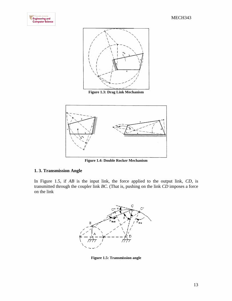
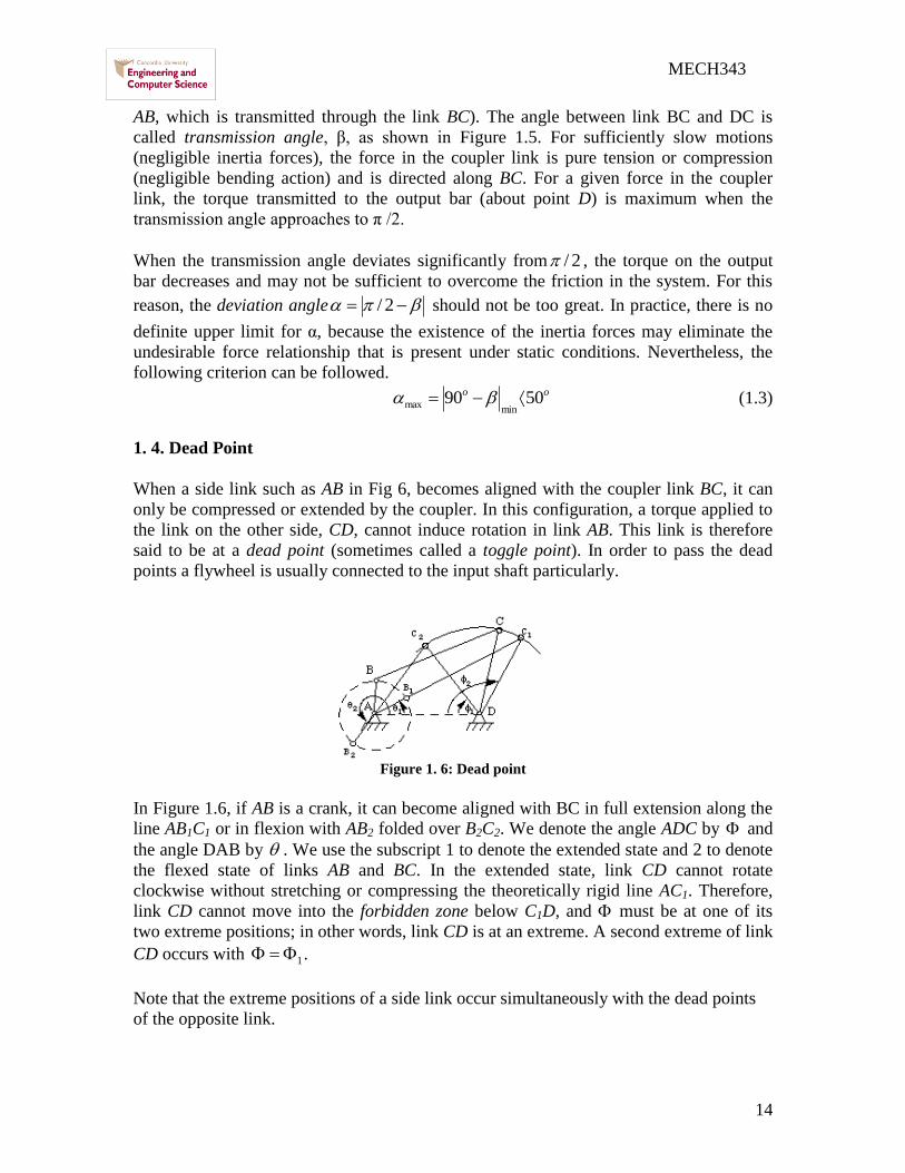
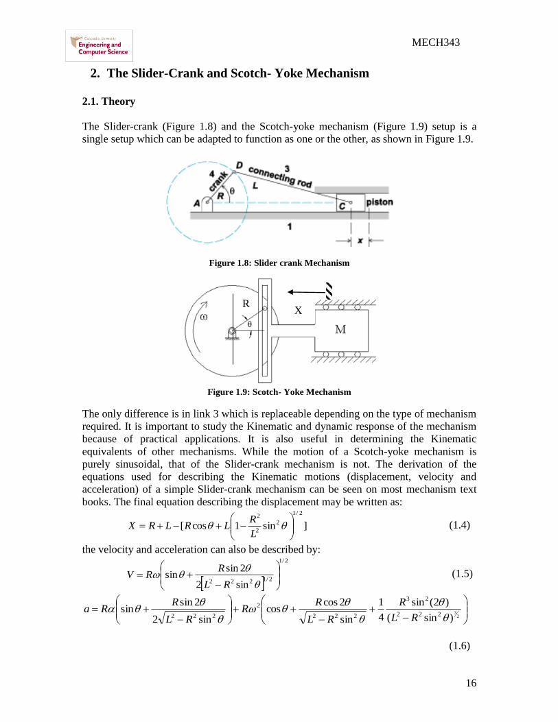
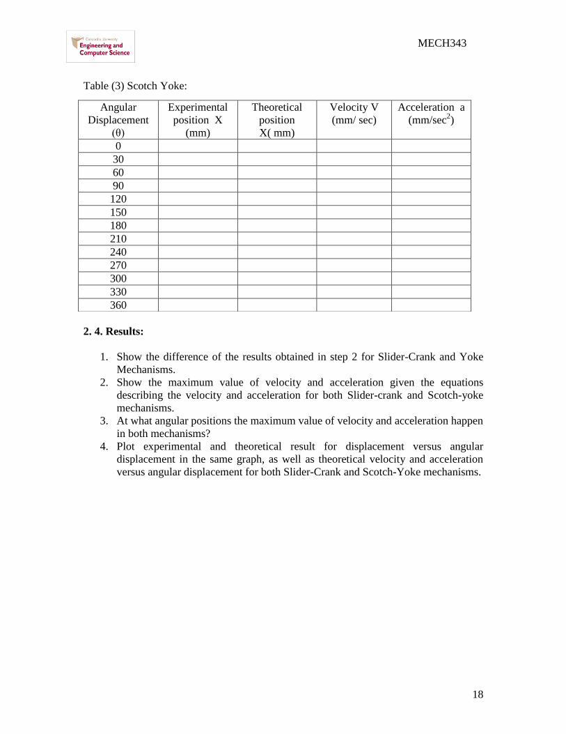
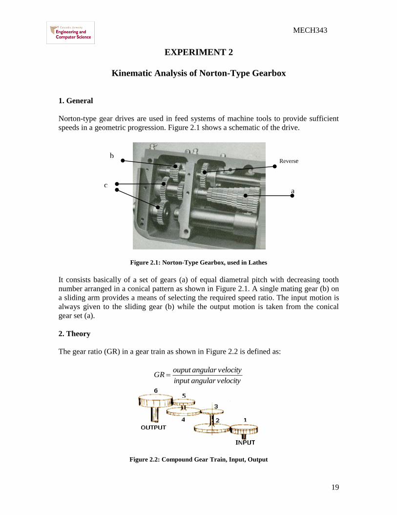
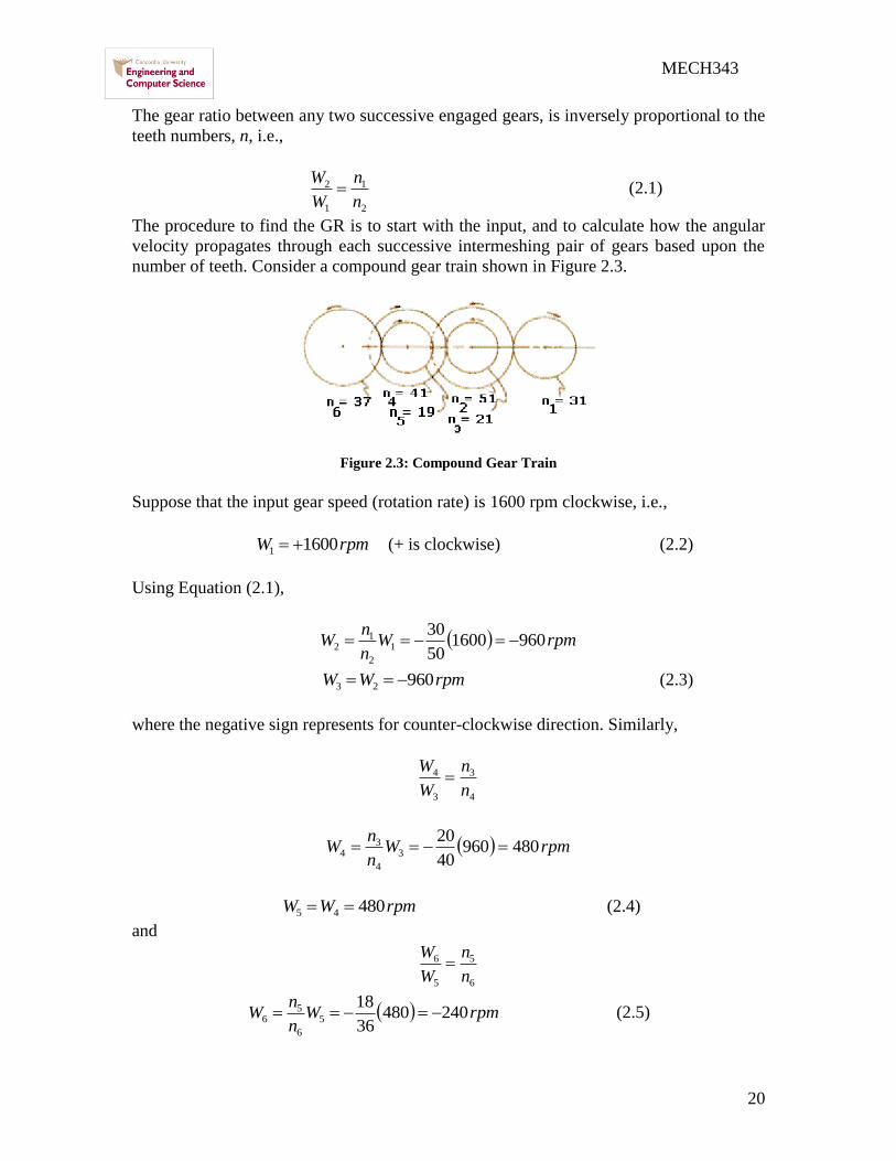
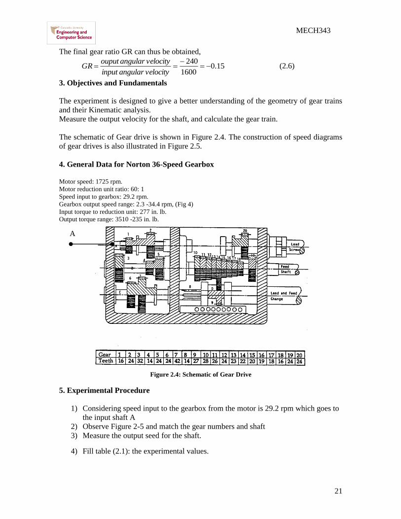
21
MECH343
The final gear ratio GR can thus be obtained
1501600
240
velocityangularinput
velocityangularouputGR (26)
3 Objectives and Fundamentals
The experiment is designed to give a better understanding of the geometry of gear trains
and their Kinematic analysis
Measure the output velocity for the shaft and calculate the gear train
The schematic of Gear drive is shown in Figure 24 The construction of speed diagrams
of gear drives is also illustrated in Figure 25
4 General Data for Norton 36-Speed Gearbox
Motor speed 1725 rpm
Motor reduction unit ratio 60 1
Speed input to gearbox 292 rpm
Gearbox output speed range 23 -344 rpm (Fig 4)
Input torque to reduction unit 277 in lb
Output torque range 3510 -235 in lb
Figure 24 Schematic of Gear Drive
5 Experimental Procedure
1) Considering speed input to the gearbox from the motor is 292 rpm which goes to
the input shaft A
2) Observe Figure 2-5 and match the gear numbers and shaft
3) Measure the output seed for the shaft
4) Fill table (21) the experimental values
A
22
MECH343
Table 2 1 Output results
Figure 25 Speed Diagram
6 Experimental Result
1) Calculate the theoretical output speed and show the calculation
2) Calculate the gear ratio for all cases
3) Plot speed diagram for the all cases depending on the one shown in Figure 2-5
Case
Input
Output (rpm)
G-10 G-14 G-16 G-18
1
1-3
3-6
Theoretical
GR
Experimental
GR
2
2-5
3-6
Theoretical
GR
Experimental
GR
3
2-5
4-7
Theoretical
GR
Experimental
GR
23
MECH343
EXPERIMENT 3
Hook (Cardan) Joint or Universal Joint
1 Introduction
The simplest means of transferring motion between non axial shafts is by means of one or
two universal joints also known as Cardan joints in Europe and Hookrsquos joints in Britain
The shafts are not parallel to one another and they may be free to move relative to one
another For this reason this very simple spherical mechanism appears in an enormous
variety of applications The most common application is Cardan joint used in the trucks
as shown in Figure 31 A universal joint is a simple spherical four-bar mechanism that
transfers rotary motion between two shafts whose axes pass through the concurrency
points The joint itself consists of two revolute joints whose axes are orthogonal to one
another They are often configured in a cross-shape member as shown in Figure 32
2 Objective of Universal Joint
Coupling is used to connect two intersecting shafts
Consists of 2 yokes and a cross-link
Figure 31 Cardan Joint used in Trucks
Figure 32 Schematic of Cardan Joint
The transmission behavior of this joint is described by Equation (31)
12 tan
cos
1arctan
(31)
where is the momentary rotation angle of the driven shaft 2
24
MECH343
Figure 33 Schematic of Cardan Joint
The angular velocity ratio can be described by
22
2
4
sinsin1
cos
(32)
where β is the angular misalignment of the shafts and Ө is the angle of the driving shaft
It is noted that
max2
4
at oo 27090
min2
4
at ooo 3601800 (33)
if β = 0 2
4
= 1 = constant at any Ө
2
4
will vary between a minimum and a maximum during each revolution
ω2 = ω4 only at 4 instants as shown in Figure 34
This is a very big disadvantage in case of automotive vehicles this means that rear
wheels will rotate at variable speed
Figure 34 Relation between
2
4
and Ө
ω2 is constant (because engine and flywheel) speed of car cannot be variable each
revolution because its inertia and so this means tires will slip and severe wear will
happen
25
MECH343
The effect of the angle β can be shown by plotting 2
4
for different values of β (Figure
35)
Figure 35 Relation between
2
4
and β
The acceleration expression of the follower of universal joint for constant ω2 is given by
222
22
24
sinsin1
2sinsincos
(34)
Recall y = u(x)v(x) therefore yrsquo= [vursquo-uvrsquo]v2
For acceleration or retardation
-acceleration when 2Ө lies between 0 -180o
-deceleration when 2Ө lies between 180 -360o
Maximum acceleration occurs when dα4 dӨ = 0 Thus
42
2
maxsin2
sin22cos
forgives
(35)
It is possible to connect 2 shafts by 2 Hooks couplings and an intermediate shaft that the
uneven velocity ratio of the first coupling will be cancelled out by the second Condition
(Figure 36)
42 (36)
Yoke 32 lies in plane containing shaft 2 3
Yoke 34 lies in plane containing shaft 3 4
Figure 36 Two shafts by two Hooks couplings and an intermediate shaft
26
MECH343
2 Objective
Testing the affect of changing of the angle between the shaft and universal joint on the
input and output shaft speed and calculate the speed ration between output and input shaft
speed
3 Experimental Procedure
1) Fixing the input shaft angle 2 0o
2) Setting the output shaft angle 154
3) Filter setting cutoff freq 4 Scope setting ch1 500mv ch2 500mv M 50ms run
scope turn on motor After stable fluctuate signal appear on screen stop scope then
turn off motor
4) Check the input and output shaft speed by using Cursor paired We assume that at
0 N4 is min setting paired cursor at this point as t=0 ms Moving cursor along
ch2 signal and record t and N4 by ∆ __ms __v Fill table 3-1 N2 is input shaft
speed It is constant
5) Repeat step 2 setting the output shaft angle 304 Fill table 3-2
6) Plot the graph of velocity ratio during one cycle for both cases Compare with
theoretical plot using equation 32
Table 3 1 Test results of Cardan joint
154
Table 3 2 Test results of Cardan joint 304
(o) 0 45 90 135 180 225 270 315 360
t (ms)
N4(v)
N2(v)
N4N2
(o) 0 45 90 135 180 225 270 315 360
t (ms)
N4(v)
N2(v)
N4N2
27
MECH343
EXPERIMENT 4
Mechanical Oscillator for Measurement of Friction Coefficient
1 Introduction
The mechanical oscillator is an apparatus which allows the experimental
determination of friction coefficient by measuring the period of an oscillating table As
shown in Figure 41 the apparatus consists of two counter rotating wheels upon which is
placed a table of uniform weight
Figure 41 The mechanical oscillator
If the center of gravity of the table is not centered when it is placed on the rotating wheels
then more of its weight will rest upon one wheel than upon the other Consequently the
frictional forces will not be equal and the table will move in the direction of the larger of
the two forces But the inertia of the table will carry it too far past the center point and the
other wheel will exert the larger frictional force Thus the table will oscillate back and
forth at a frequency which depends upon the coefficient of friction
The basic step to find the equation of motion of the system is to construct the Free Body
Diagram of the oscillating table Figures 2(a) 2(b) and 2(c) show this procedure
Summing the forces in the horizontal plane we have
0RRXg
W21 (41)
or
0XL
W2X
g
W
(42)
hence
0XL
g2X
(43)
28
MECH343
Figure 42 procedure of finding the equation of motion
Since the differential equation of motion of free vibration for a one degree of freedom
system is of the form
02 XX n (44)
where n is the natural frequency of the system then
L
g22
n
(45)
But L
gfn
24 222 (46)
where
f = the frequency of the oscillating table in cps
L = the distances between wheel centers in ft
g = gravity constant
hence 2
22f
g
L (47)
The solution of the equation of motion can be written in the form
tBtAX nn cossin (48)
With the initial condition
00 XandXXt O (49)
one gets oXBandA 0 (410)
The response of the oscillating table is therefore
tL
gXX o
212
cos
(411)
29
MECH343
tL
g
L
gXX o
21212
sin2
(412)
tL
g
L
gXX o
212
cos2
(413)
Thus it may be concluded that the response of the oscillating table is governed by the
initial displacement X0 the coefficient of friction micro and the difference between wheel
centers L
2 Objectives
The experiment is designed to illustrate some of the direct applications of the
theory of vibration to the measurement of physical quantities The experiment also
demonstrates the differences between mathematical models and actual physical systems
Calculate the friction coefficient between the wheels and the bars
3 Description of Experiment
The oscillating table apparatus consists of four grooved wheels mounted on two
axels which are driven by a 120 HP electric motor and a gear reduction unit in opposite
directions The table consists of circular rods connected in a rectangular shape such that
the rods are guided by the grooved wheels
4 Experimental Procedure
1) Measure L the length between the centers of the two wheels
2) Locate one of the bars on the wheels
3) Select two different speeds for the wheels and when it starts rotating and the bar
moving calculate the time for 10 oscillations
4) Calculate the experimental coefficient of friction μ through the following
equation 2
22f
g
L When f is the frequency g gravity acceleration L the
length between the centers of the two wheels Fill table 4-1
5) Find the theoretical coefficient of friction μ for all bars
6) Compare between theoretical and experimental coefficient of frictions μ
Table 4 1 Combinations for measuring the friction coefficient
Case Material of
the bar
Speed
(rpm)
Time taken
for 10
oscillation
Frequency
(f)
Coefficient
of friction
(micro)
Standard
coefficient
of friction
1 Steel
2 Brass
3 Aluminum
30
MECH343
EXPERIMENT 5
5-1 PLANETARY GEAR TRAIN KINEMATICS
1 Introduction
A planetary gear train is one in which the axis of some of the gears may have motion A
planetary gear set always includes a sun gear one or more planet gears and a planet
carrier or arm which sometimes called as sun-and-planet planetary gear train as shown in
Figure1
Figure 51 Planetary gear train
A planetary gear set as shown in Figure 52 is one having two degrees of freedom This
means that the motion of each and every element of the mechanism is not defined unless
the motion of two of its elements is specified To make the planetary set a one degree of
freedom gear train one must fix the motion of one element of the mechanism
Figure 52 Sun-and-planet planetary gear train
2 Solution of Planetary Trains by Formula Methods
Figure 53 shows a planetary gear set which is composed of a sun gear 2 an arm 3 and
planet gears 4 and 5
31
MECH343
Figure 53 Compound Planetary Gear Set
We can express the velocity of gear 2 relative to the arm 3 in the form
3223 nnn (51)
3553 nnn (52)
Dividing Equation (52) by (51) gives
32
35
23
53
nn
nn
n
n
(53)
Since this ratio is the same and is proportional to the tooth numbers it is equivalent
therefore to the train value e
32
35
nn
nne
(54)
Or AF
AL
nn
nne
(55)
where nF = rpm of first gear in train
nL = rpm of last gear in train
nA = rpm of arm
The experiment is designed to demonstrate the fundamentals of planetary gear train and
to show all possible motions that can be obtained with this type of gear trains
3 Objective
Calculate the gear train ratio for the planetary gearbox and the degrees of
freedom that the system has
4 Experimental Procedure
For the planetary gear trains mechanism shown in Figure 51
1) Calculate the degree of freedom to the planetary gear system
2) Calculate the gear train ration through the following equation
21
23
nn
nne
When the outer ring is fixed
When the planet gears are fixed
32
MECH343
5-2 The Borg-Warner Model 35 Automatic Transmission
Simulator
1 Introduction
The Borg-Warner Model 35 Automatic Transmission comprises a three element
torque converter--coupling and a planetary gear set to provide three forward ratios and
reverse
The planetary gear set consists of two sun gears two sets of pinions a pinion
carrier and a ring gear
Power enters the gear set via the sun gears In all forward ratios power enters
through the forward sun gear In reverse it enters through the reverse sun gear Power
leaves the gear set by the ring gear and the pinions are used to transmit power from the
sun gears to the ring gear
In reverse a single set of pinions is used which causes the ring gear to rotate in the
opposite direction from the sun gear In forward ratios a double set of pinions is used to
cause the ring gear to rotate in the same direction as the sun gear
The Carrier locates the pinions relative to the two sun gears and the ring gear also
forming a reaction member for certain conditions The various mechanical ratios of the
gear ser are obtained by the engagement of hydraulically operated multi-disc clutches and
brake bands
Power flow in each ratio is achieved by locking various elements of the planetary gear set
as follows
1st Gear (Lockup selected)
The front clutch is applied connecting the converter turbine to the forward sun
gear The rear band is also applied holding the pinion carrier stationary The gear set
provides the reduction of 239 l The reverse sun gear rotates freely in the opposite
direction to the forward sun gear
33
MECH343
1st Gear (Drive selected)
The front clutch is applied connecting the converter turbine to the forward sun
gear The one-way clutch is in operation preventing the pinion carrier from moving
opposite to the engine rotation The gear set again provides the reduction of 239 1 On
the overrun the one-way clutch unlocks and the gear set freewheels
2nd Gear (Lockup or drive selected)
Again the front clutch is applied connecting the converter turbine to the forward
sun gear The front band is applied holding the reverse sun gear stationary The pinions
now walk around the stationary sun gear and the gear set provides the reduction of 145
l
3rd Gear (Drive selected)
Again the front clutch is applied connecting the converter turbine to the forward
sun gear The rear clutch is applied connecting the turbine also to the reverse sun gear
Thus both sun gears are locked together and the gear set rotates as a unit providing a
ratio of 1 1
Neutral and Park
The front and rear clutches are released and no power is transmitted from the
converter to the gear set
Reverse
The rear clutch is applied connecting the converter turbine to the reverse sun gear
The rear band is applied holding the pinion carrier stationary providing a reduction of
209 l
2 Gear Ratios
119866119890119886119903 119877119886119905119894119900 120579119900120579119894
=1
239
The carrier is held stationary to provide the
reaction member and the gears operate as a
Simple gear train
34
MECH343
The reverse sun gear is held to that the gears
now operate as an epicyclic gear train
For an epicyclic gear train shown as following
119866119890119886119903 119877119886119905119894119900 120579119900120579119894
=1
145
119894134 =
1205961 minus 1205964
1205963 minus 1205964= minus
11988521198851
11988531198852prime
119900119903 120596119871
32
67= 120596119869 minus 120596119871 120596119869 =
99
67120596119871
For our transmission show as above
119894119865119869119871 =
120596119865minus120596119871
120596119869minus120596119871= minus
119885119866
119885119865
119885119867
119885119866
119885119869
119885119867=
67
28 (1)
119894119865119870119871 =
120596119865minus120596119871
120596119870minus120596119871= minus
119885119866
119885119865
119885119867
119885119866
119885119870
119885119867= minus
32
28 (2)
Hence minus120596119871
120596119869minus120596119871= minus
67
68
28
32
From (2) 120596119865 minus 120596119871 =32
28 120596119871 120596119865 =
60
28120596119871
Therefore 119894119865119869 =120596119865
120596119869=
60
28
67
99= 145021645
So 120579119900
120579119894=
1
145
35
MECH343
119866119890119886119903 119877119886119905119894119900 120579119900120579119894
=1
1
Both sun gears are locked together and the
gears set rotates as a unit
119866119890119886119903 119877119886119905119894119900 120579119900120579119894
=1
209
With the reverse gear engaged power is
applied to the reverse sun gear The planet
carrier is held stationary so that the planet
gears rotate the ring gear in the opposite
direction to the reverse sun gear
36
MECH343
3 Experimental Procedure
Pins and slotted plates represent the multi-disc clutches and brake bands The various
gear ratios of the gear set may be obtained by inserting the appropriate pins as indicated
below
A B C D E F
Lockup 1Drive 1
Lockup 2Drive 2
Drive 3
Reverse
Neutral
Park Note
1 Lose all pin and turn input shaft and output shaft make sure input shaft disk and
output shaft disk indicate to 0 then lock pins for each case
2 Turn input shaft one turn (360 ) read output disk (degree)
3 Fill out following table
Input (degree) Output (degree)
Lockup 1Drive 1 360
Lockup 2Drive 2 360
Drive 3 360
Reverse 360
4 Results
According to power flow and gear ratio figures for each case referring to 2nd gear
ratio calculation derive and calculate gear ratios for 1st 3
rd and reverse shift Compare
them with your experimental results
37
MECH343
EXPERIMENT 6
Static and Dynamic Balancing
1 Objective
The objectives of this experiment are
Understanding the concept of static and dynamic balancing
Understanding unbalance torque
Justifying theoretical calculation for balancing with experiment
Balancing the shaft by the four given masses
2 Introduction
Unbalanced dynamic forces effects have profound influence on the working and
of rotating machinery like turbines compressors pumps motors etc These forces act
directly on the bearings supporting the rotor and thus increase the loads and accelerate the
fatigue failure These unbalanced forces induce further mechanical vibrations in the
machinery and connected parts thereby creating environmental noise problem through
radiation of sound Hence it is desirable to balance all such uncompensated masses and
thus reduce the effect of unbalance forces in a dynamics balancing machine
Balancing is the technique of correcting or eliminating unwanted inertia forces which
cause vibrations which at high speeds may reach a dangerous level An important
requirement of all rotating machinery parts is that the rotation axis coincides with one of
the principal axis of inertia of the body After a roll is manufactured it must be balanced
to satisfy this requirement especially for high speed machines The condition of
unbalance of a rotating body may be classified as static or dynamic unbalance
2 1 Static Unbalance
An idler roll is statically balanced if the roll doesnt rotate to a heavy side when free to
turn on its bearings Thus the rolls center of gravity is on the axis of rotation Static
unbalance (Figure 61) creates a centrifugal force when rotating which causes deflection
of the roll Idler rolls are sometimes static
balanced only when the roll operates at slow
speeds
The static unbalance usually happens because
of errors in the manufacturing tolerances of
the rotating parts Therefore static imbalance
is essentially a weighing process in which the
part is acted upon by either gravitational or
centrifugal force This type of unbalance
could be easily reduced or removed by static
balancing
Figure 61 Static (or force) Unbalance
38
MECH343
2 2 Dynamic Unbalance
An idler roll may be in perfect static balance and not be in a balanced state when rotating
at high speeds A dynamic unbalance is a ldquocouplerdquo or twisting force in two separate
planes 180 degrees opposite each other (Figure 62) Because these forces are in
separate planes they cause a rocking motion from end to end A roll that is unbalanced
will cause 1) machinery vibrations 2) web
flutter and 3) a decrease in bearing life due to
unnecessary forces
To dynamically balance a roll it must first be
statically balanced Then the roll must be
rotated to its operating speed and have the
dynamic unbalance eliminated by adding or
subtracting weight The determination of the
magnitude and angular position of the
unbalance is the task of the balancing
machine and its operator Balancing
machines are provided with elastically
supported bearings in which the idler roll may
spin Because of the unbalance the bearings
will oscillate laterally and the amplitude and
phase of the roll are indicated by electrical
pickups and a strobe light
Figure 63 shows a long rotor which is to be mounted in bearing A and B We might
suppose that two equal masses m1 and m2 are placed at opposite ends of the rotor and at
equal distances r1 and r2 from the axis of rotation Since masses are equal on opposite
sides of the rotational axis the rotor is statically balanced in all angular positions But if
the rotor is caused to rotate at an angular velocity ω radsec the centrifugal forces m1r1ω2
and m2r2ω2 act respectively at m1 and m2 on the rotor ends These centrifugal forces
produce the equal but opposite bearing reactions FA and FB and the entire system of
forces rotate with the rotor at the angular velocity ω Thus the rotor is to be statically
balanced and at the same time dynamically unbalanced
Figure 63 Dynamically Unbalanced Rotor
Figure 62 Dynamic (or couple) Unbalance
39
MECH343
3 Principle and Theory of Operation
Consider a body of mass M rotating with a uniform angular velocity about O with
eccentricity e as shown in Figure 64 The centrifugal force Fc acting on the axis of
rotation is Me2 This force is therefore very sensitive to speed and hence there is a need
to reduce this force either by operating at lower speeds or by decreasing the eccentricity
as shown in Figure 65
O
e
M
M e
2
Figure 64 Unbalanced Disc
Center of rotation
( new center of
gravity )
Rotating Disc Added mass m
Center of gravityOriginal center
of gravity
(a) (b)
Figure 65 Illustration of The Simplest Method of Static Balancing
In general it is desirable to make e as low as possible If the rotor thickness to diameter
ratio is less than 05 and speed are below 1000 rpm the rotor can be single plane
balanced - otherwise two-plane balancing is necessary In the single plane balancing
technique with a rotor of mass mi and radius ri from the axis of rotation and lying in the
same plane the condition for static balance is used
0~iirm (61)
where i = 1 2 which denotes the total number of masses and m denotes the mass The
vector ir~ represents the eccentricity e of the mass mi from the axis of rotation
When the bodies are rotating in several planes the condition for dynamic balance has to
be satisfied in addition to that for static balance This is given by
0~~ iii rzm (62)
where iz~ is the axial coordinate vector of the mass mi measured for a chosen datum In
the two-plane balancing technique instead of satisfying Equations (61) and (62)
40
MECH343
explicitly Equation (62) is used with two different datum planes for iz~ Mathematically
if the distance between these two plane is oz~ then
0~)~~( ioii rzzm (63)
It is therefore clear that Equations (62) and (63) imply the satisfaction of Equation
(61) Conceptually it means that if a system of bodies rotating in several planes is in
dynamic balance with respect to two different datum planes then the system is also in
static balance This is the principle of the two-plane balancing technique
4 Description of Experimental Apparatus
Figure 66 shows the Static and Dynamic Balancing Apparatus It consists of a perfectly
balanced shaft with four rectangular blocks clamped to it The shaft is mounted in ball
bearings and it is driven by a 12 volt electric motor through a belt and pulley drive The
shaft assembly is mounted on a metal plate resting on four resilient rubber supports
which allow the mount to vibrate when the shaft is not balanced
The rectangular blocks can be clamped to the shaft at desired out-of-balance moments by
means of discs having eccentric holes of various diameters The discs are fixed to the
blocks by hexagon socket set screws Any longitudinal and angular position of a block
relative to the shaft can be set by linear and protractor scales provided Adjacent to the
linear scale is a slider which can be pushed against the block to read its longitudinal
position The slider also serves as a datum stop against which the blocks can be held
when reading their angular position on the shaft
The out-of-balance moments are measured by fitting the extension shaft and pulley to the
main shaft Each rectangular block is then clamped to the shaft in succession A cord with
a weight bucket at each end is hung on the pulley and bearing balls are placed in the
bucket until the block has turned through 90deg The out-of-balance moment is proportional
to the number of balls required
to turn the block
A Perspex dome serves as the
safety cover The shaft cannot
be driven unless the dome is in
position which is achieved by
micro switches actuated by the
dome The motor switch on the
front panel is spring loaded so
that the motor cannot be left
running The motor requires a
power supply of 12 volts at 2
amperes which is provided by
E66E90 speed controller
Figure 66 Static and Dynamic Balancing Apparatus
41
MECH343
5 Experimental Procedure
5 1 TEST 1 Static Balancing
1 Looking at the shaft from the side the masses will be as shown in figure 6-7
each mass has an angle θ with horizontal
Figure 6-7 Shaft view from the side
2 The masses forces are given by the following table 6-1
The masses values Table 6-1
3 In order to balance the shaft statically the sum of the forces will be equal zero
as the following equations
sum F=0
F1cos θ1+ F2cos θ2+ F3cos θ3+ F4cos θ4=0 (1)
F1sin θ1+ F2 sin θ2+ F3 sin θ3+ F4 sin θ4=0 (2)
4 Since we have just two equations with four unknown angles we assume
θ1=0ordm θ2=90ordm
5 Solving the two equations or using force polygon by AutoCAD to find the θ3
θ4
5 2 TEST 2 Dynamic balancing
1 Looking for the shaft from in front the masses create the forces as shown in
figure 6-8 each mass has an arm X create a momentum
F1
F2
F3
F4
42
MECH343
2 In order to balance the shaft dynamically the sum of the momentum will be
equal zero as the following equations
sum M=0
F1cos θ1X1+ F2cos θ2X2+ F3cos θ3X3+ F4cos θ4X4=0 (1)
F1sin θ1X1+ F2 sin θ2X2+ F3 sin θ3X3+ F4 sin θ4X4=0 (2)
3 Since we have just two equations with four unknown arms we assume
X1=50 mm X2=100 mm
4 Solving the two equations or using momentum polygon by AutoCAD to find
the X3 X 4
TABLE 6 2
Block 1 2 3 4
Mass 88 82 74 64
Angle θ(ordm) 0 90
Arm X (mm) 50 100
6 Typical Calculations
The basic equations that are used for balancing purposes are
0rW ii (63)
0rWa iii (64)
Suppose that block (1) is placed 17 mm from the left end of the shaft at zero angular displacement and that
block (2) is placed 100 mm from it at 120deg The measured out-of-balance moments are as follows
Figure 68 In front shaft view
43
MECH343
TABLE 6 3 OUT-OF-BALANCE MOMENTS
It is first necessary to draw the moment polygon of Wr values as shown in Figure 68 to determine the
angular positions of blocks (3) and (4) W1r1 and W2r2 are known in both magnitude and direction The
vector W1r1 has been drawn at positive X-direction (θ = 0) The lengths of vectors W3r3 and W4r4 are known
and arcs can be drawn from the ends of W1r1 and W2r2 to get the directions of the unknown vectors
Figure 69 shows the diagram of the angular positions and the corresponding longitudinal locations of the
blocks on the shaft are 17 mm for the first 117 mm for the second block
To find the longitudinal positions of the other two blocks we designate distance of block (3) by a3 and
distance of block (4) by a4 measured from block (1) so block (1) is the reference and will not appear in
calculations
Draw a vector a2W2r2 = 100 (82) units long parallel to r2 and vectors a3W3r3 and a4W4r4 parallel to r3 and r4
respectively so that the moment polygon is closed The lengths of vectors a3W3r3 and a4W4r4 can be
measured and the magnitudes found by using the scale factor From these a3 and a4 can be calculated
Notice that the sense of vector a3W3r3 is reverse In order to maintain vector a3W3r3 the only possible
solution is to reverse a3 So from the vector polygon (triangle) it follows
a3 = -12 mm
a4 = 124 mm
This means that block (3) should be located 5 mm from the left end of the shaft The blocks should be
positioned as follows
Block Angular Position (Deg) Longitudinal Position (mm)
(1) 0 17
(2) 120 117
(3) 190 5
(4) 294 141
The values of a3 and a4 can be found analytically using complex vector approach
Real and imaginary components yield
100(82) cos 120deg + (74) a3 cos 190deg + (64) a4 cos 294deg = 0
100(82) sin 120deg + (74) a3 sin 190deg + (64) a4 sin 294 deg = 0
which reduce to
4100- 7288 a3 -2603 a4 = 0
71014- 1285a3 -5847 a4 = 0
44
MECH343
Solving the two equations gives a3 = -1194mm a4 = 12396mm
The values compare very well with those obtained graphically
In order to obtain independent results it is suggested that Wr values of the blocks are varied by using
different positions of the discs with eccentric holes The angular displacements between blocks (1) and (2)
may also be varied
Figure 69 Moment Polygon of Wr
45
MECH343
EXPERIMENT 7
Machine Fault Simulator (MFS)
1 Theory
Refer to experiment number 6
2 Description of Experimental Apparatus
Figure 71 shows the machine fault simulator The rotor is driven by a variable speed
motor via a flat belt and the rotor rotational speed is captured through a digital
tachometer The vibration due to the unbalanced rotor is measured and fed directly into
the on-board processor of the machine
Figure 71 Machine Fault Simulator
3 Objective
In this experiment we will study the reaction of the shaft and the motor when the shaft is
balanced and when it is unbalanced
4 Experimental Procedure
1) Run the Vibro-Quest Software
o Define a ldquoNew Projectrdquo (under root)
o Fill up the window select ldquoProject namerdquo click ldquoNextrdquo
o Select ldquoNonerdquo from the menu on the right side click ldquoNextrdquo
Belt
Motor
Disk A Disk B
Reciprocating
Mechanism
Speed
Control
46
MECH343
o Review the table (do not change the default) click ldquoNextrdquo
o Review the table check the setting data click ldquoNextrdquo
o Click ldquoDonerdquo
o Review the information provided if they are not ok ldquoGo backrdquo to modify
the data then click ldquoFinishrdquo
2 Select ldquoDatardquo from the toll bar on the computer
3 Name the ldquoTest Titlerdquo in the window Insert the parameters used in the test and
click ldquoNextrdquo
4 Review the information provided in the window and click ldquoNextrdquo
5 Chose 2000 as Frequency limit 1600 for Space line Leave the rest information as
defaulted and ldquoGO DAQrdquo
2) Running the Machine Fault Simulator
Select the required speed (rpm) change it to frequency (Hz) using the following
relation 60)rpm(n2)Hz(f
1 Run the machine using speed control system at desired speed
2 Wait about 15 seconds to stable the system
3 Click onrdquo START RECORDINGrdquo
4 When the recording is finished save the file under the root of ldquoDatardquo of base line
at the subdirectory that you want to compare with the other data (for example if
you are running the machine at 20 Hz save the your file under 20 Hz subdirectory)
5 Now select the ldquoProject namerdquo from the left menu all the relevant tests will
appear at the right table under the ldquoTest Explorerrdquo
6 To compare the data from different files Hold down the ldquoShiftrdquo key and select
any two interested files that you are going to compare
7 Click on ldquoComparerdquo to observe the difference between the unbalanced system
with a base system
8 To observe more clearly the difference between the frequency responses of the
different test click on ldquoOverlayrdquo
TEST 1 Imbalance Effects on Vibration response
Install the defined weight in one of the taped hole in rotor disk A and tight it
securely with a nut
Close the cover of MFS
Change the motor speed and record vibration level at each bearing For this
purpose you don not need to define new project for each speed define a new
project( follow steps 1-6 from section 3) then follow steps 1-2 for each speed
from section 4
Measure the average level of amplitude at each speed and Plot it against the speed
Repeat steps 2-5 for 2 different weights at 2 different radius and angles
47
MECH343
TEST 2 Balancing the Imbalance Rotor
Add weight at different radius and angles using the ldquosample calculationrdquo to
balance the rotor
If the rotor is balanced define a ldquoNew projectrdquo and follow steps 3-8 of Section 4
Fill Table 7 1
TABLE 7 1
Unbalance weight on disc A ____________ angular position _______________
Mass Added on disk B gr r (mm)
Amp baseAmp New
48
MECH343
EXPERIMENT 8
DETERMINATION OF SPUR GEAR EFFICIENCY
1 Objective
The main objective of the experiment is to determine the efficiency of the
Spur gear and worm gear unit
2 Introduction and theoretical background
21 Pinion gear
Two intermeshed toothed wheels make up a pinion gear This type of gear
permits a positive transmission of motion and torque Wheel pairs are available in
different shapes and shaft configurations Figure 1 explains the various types of gears and
their arrangements
Fig8 1 Various types of gear arrangements
22 Worm gear
A worm gear is a screw-type transmission unit whose axes generally intersect at
right angles The worm and wheel make contact on a straight line Normally the worm
has a cylindrical core and the wheel globoid toothing Units with a very high performance
49
MECH343
consist of a globoid worm and globoid wheel A worm gear with a cylindrical worm has
the following special features
High load capacity compared with spur gears due to linear contact
Low-noise operation and high absorption of vibrations
Wide transmission range down to low ilt110
High efficiency at high transmission ratios high efficiencies(η le 98 ) can be
achieved with very sophisticated designs under favorable operating conditions a
decrease in pitch angle (high transmission ratio) or speed is accompanied by a
corresponding decrease in efficiency (to η le 50 )
Self-locking operation
Smaller and lighter design compared with spur bevel gear units possessing high
transmission ratios
23 Basic definitions
Drive torque
The drive torque is the product of the force F and the lever arm l on which the
force acts
M = F X l (1)
M is in Nm F is in N and l in m
Drive power
The drive power of a rotating shaft is the product of the torque M and angular
frequency ω P = M X ω (2)
and 60
2 n (3)
P is in W n is in rpm
Efficiency
The efficiency is defined as the ratio between the output and input powers It has a
maximum theoretical value of 1
in
out
P
P (4)
where speed i
nn 1
2
50
MECH343
3 Experimental set-up
Figure 2 shows the complete view of the experimental set up
Fig8 2 Complete view of GUNT AT 200 experimental set up
The modules comprising the drive unit spur gear worm gear and magnetic
powder brake are mounted on a profile frame The DC shunt motor is designed for right-
hand and left-hand rotation The drive unit is electrically powered via control housing
The control unit adjusts the DC machinersquos speed via its armature voltage Its target speed
is set by means of a potentiometer on this housing Its actual speed is measured and
indicated by means of an inductive proximity switch and evaluation unit The speed is
51
MECH343
measured inductively by a contactless sensor disc and indicated by a digital display
element on the control unit Electronic thyristor speed control with I x R compensation
provides a high torsional rigidity The reaction torque exerted on the drive housing is
measured by means of a spring force meter connected to a lever arm
The transmission units consist of a 2-stage spur gear with transmission
ratio i = 135 and a single-stage worm gear with transmission ratio i = 14The
transmission torque can be determined on the drive side as well as the brake side To
facilitate adjustment of the brake torque the brake characteristic (current torque) is
recorded in a preliminary experiment Moments are determined through power
measurements (spring balance) with a known lever arm The moments measured input
speeds and transmission ratios are used to determine power and efficiency
The magnetic powder coupling consists of two independently mounted
rotors ie a primary and a secondary rotor both furnished with ball bearings The
primary rotor also serves as a coil carrier If one of these two rotors is deactivated the
magnetic powder coupling can also be used as a brake The air gap between the two
rotors contains a special magnetic powder If a direct voltage is applied to the excitation
winding the powder aligns itself with the resulting magnetic field lines to form a
compact mass providing a frictional link between the primary and secondary rotors The
value of the torque depends on the adjusted current When the current-proportional
moment is exceeded slippage occurs without any transition
4 Experiments procedure
As shown in Figure 82 the complete view of the experimental set up for this
experiment there is input as the motor speed and the output as excitation current so that
there is two steps for this experiment
After making sure spur gear is connected as shown in Figure 83
1) Fix the output excitation current at I= 50 mA and change the speed of the motor as
shown in the table (1) each time measure the motor force F1 and the brake force F2
52
MECH343
Figure 83 Configuration of spur gear unit experimental set up
Measurement data to determine the efficiency of Spur gear unit Table (1) I = 50mA
SlNo Motor speed
( n1 ) rpm
Motor holding
force ( F1 ) N
Brake holding force
( F2 ) N
Efficiency ( η )
1 500
2 1000
3 1500
4 2000
5 2500
In order to find out the spur gear efficiency we go through the following equations
The general equation for the spur gear efficiency is
in
out
P
P
The drive power of a rotating shaft is the product of the torque M and angular
frequency ω P = M X ω
The drive torque is the product of the force F and the lever arm l on which the
force acts
M = F Arm
When the arm for the motor Arm1=25 mm and for the brake Arm2=50 mm
53
MECH343
And the angular velocity from the following equation
60
2 n
In order to find the speed for the brake we use this ratio assuming i= 135
i
nn 1
2
2) Fixing the input n1= 1500 rpm and changing the output and filling table (2)
Recorded values of the excitation current and the force on the lever arm table (2)
Speed n1= 1500 rpm
Excitation current I (mA) Force F2 on the lever arm (N)
50
70
90
110
130
150
130
110
90
70
50
5 Experiments Results
1) Plot the characteristics curve between the current I and the force on the lever arm
F2
2) Plot the characteristics curve between the current I and the torque M
3) Determine the efficiency of the spur gear unit Comment on the errors on the
efficiency if the calculated efficiency deviates from the realistic values of 80 -
90
54
MECH343
EXPERIMENT 9
ANALYSIS OF LINKAGE MECHANISM
Try to build a linkage mechanism as the figure below
Steps
1 Turn on grid line from View-workspace-grid lines as below
2 Select rectangle tool
55
MECH343
3 Click and drag a small rectangle
4 Click the rectangle copy it (CTRL+C) paste it (CTRL+V) two times
5 Change the length of each rectangle by selecting it and writing down the desired
length in the text box named W
Make the length as (3 ndash 332 - 4)
56
MECH343
6 Use the rotate tool and the select tool to arrange the rectangles
Make sure that the spacing is 4 units as shown below
7 Put a motor at the lower end of the left link
- First select the motor - Then click at the desired point
57
MECH343
8 Put a pin joint at the lower end of the right link
- First select the pin joint - Then click at the desired point
9 Put a point element at the remaining ends
- First double click (this
enable you to assign multiple
points) on the point element
It should look like below
58
MECH343
10 Join the links by selecting two points then selecting Join
Click the arrow select tool
Select first point ndash
press SHIFT and
click the other point
Press
Join
They should look like
below
11 Repeat the same for the remaining two points Your model should look like below
59
MECH343
12 Click RUN ( ) and watch it rotating
13 Now we want to capture the velocity of the joint between the left link and the middle
one
- Select it and click on Define ndash Vectors-
Velocity
Click Run and watch the velocity change
Note that by clicking on the link itself and defining the velocity the program calculates
the velocity of the CG of the link
14 Now you are ready to try different measurements
Acceleration Total Force Gravitational Force
60
MECH343
15 Select a link and use the measure tool
X- Position Graph
Y- Position Graph
61
MECH343
Measuring velocity values
16 Now try to change the length of any of the links and RUN the model and observe
for any change if any and explain
17 Change the mass of any of the links and observe for any change in velocity and
force And Why if there is any
18 Now double click on the motor (resetting the mass for any link that has been
changed) and notice that the value for velocity is 1 radsec Change this to make it the
same value for acceleration and torque Write what you observe and try to explain
19 Now increase the mass for one link (eg left one) gradual and see how this will
affect the motion for a fixed value for torque velocity or acceleration of the motor
20 Now replace the middle link with two links connected with total length as the
middle one run observe and explain
21 Based on (20) search for what is the equation relation or rule that governs the
mechanism motion
62
MECH343
EXPERIMENT 10
NUMERICAL DYNAMIC SIMULATION FLYWHEEL
Problem Definition
In the two cycle piston engine shown explosive gases are
ignited in the combustion chamber above the piston The
explosions apply a force of 150 N for the duration of every
downward stroke The engine is equipped with a speed
limiting device (rev limiter) which prevents the rotational
speed from exceeding a set value (red-line) The masses of
the piston and connecting rod are 075 kg and 15 kg
respectively The mass of the crankshaft-flywheel assembly
is 30 kg Given that the red-line of the engine is 35 radsec
(340 rpm) Assume the crankshaft-flywheel assembly can
be modeled as a circular disk
Objective
Determine the forces at the crankshaft bearing (point A) and connection rod (point B)
bearing
Solution
1 INTRODUCTION
Engines that exceed the manufacturers maximum speed (over-revving) may be subject to
excessive wear and possible failure To prevent over revving internal combustion
engines are often fitted with a device known as a rev-limiter When an engine exceeds its
red-line rev-limiters interrupt the ignition system slowing the engine down Once the
speed drops below the maximum the ignition system is switched back on In this exercise
you will model an internal combustion engine equipped with a rev-limiter The engine
has three bodies the piston the connecting rod and the crankshaft The piston will be
modeled by a square body The connecting rod will be modeled by a rectangular body
The crankshaft will be modeled as a circular body The bodies will be drawn sized and
joined to each other and the background The pistons cylinder walls will be modeled with
a keyed slot joint The force of combustion will be modeled by a force attached to the top
of the piston The resulting forces at the bearings will be measured
2 SETTING UP THE WORKSPACE
For this exercise three changes in the workspace will be made First for clarity the x-y
axes will be displayed The unit of distance will also be changed from meters (default) to
millimeters
63
MECH343
If the x-y axes are not currently displayed choose Workspace from the
View menu and choose XY Axes from the Workspace submenu The x-y
axes provide a reference frame for building a simulation
Choose Numbers and Unitshellip from the View menu The Numbers and
Units dialog appears
Click the More Choices button The dialog box expands
Click and hold in the Distance field (Figure 1) The pop-up menu appears
Choose millimeters from the Distance pop-up menu
Click in the Rotation field and choose Radians from the pop-up menu
Click OK
3 CREATING THE COMPONENTS
This exercise has three objects a 15 kg connecting rod a 075 kg piston and a 30 kg
crankshaft (see Figure 2 below) The connecting rod will be modeled by a thin rectangle
400 mm in length Its width will be thin 150 mm so it closely resembles the actual
connecting rod The crankshaft as stated in the exercise is modeled as a circular disk
with a 200 mm radius and a mass of 30 kg A 200 mm square object will represent the
piston The objects will be created sized and initialized in the following steps
Creating the Crankshaft
The crankshaft is represented by a circle with a radius of 200 mm and mass of 30 kg
These parameters will be set using the Geometry and Properties utility windows
I To draw the crankshaft
64
MECH343
bull Click the Circle tool in the Toolbar
bull Click once on the background Move the mouse to expand the circle and click
again to complete sketching
II To set the mass of the crankshaft
Choose Properties from the Window menu
Click the mass field and enter the value 30
III To set the size of the crankshaft
Select the crankshaft if it not already selected
Click the Radius field (labeled ldquorrdquo) of the Coordinates bar and enter the value 200
(Figure 3)
IV Zooming In
The circle will appear small after sizing To make the rectangle easier to manipulate and
appear larger the workspace will be magnified using the Zoom tool To zoom in
Click the Zoom In tool in the Toolbar
Click near the circle The objects in the window are magnified by a factor of two with
each click of the mouse To zoom out while the Zoom In tool is selected hold down
65
MECH343
the Shift key (the magnifying glass pointer changes to ldquo-rdquo) and click Your screen
should be similar to Figure 4 below
Figure 4 The workspace after zooming in
Click the Arrow tool in the Toolbar or press the spacebar to deselect the Zoom In
tool
Creating the Piston
For this exercise the piston will be modeled as a 200 mm square with the mass of 75 kg
The Square tool will be used to draw the piston and the Properties window will be used
to set its mass
I To draw the piston
Choose the Square tool in the Toolbar On systems the Square tool is ldquohiddenrdquo in the
RectangleSquare pop-up palette by default Click and hold on the Rectangle tool to
bring the pop-up palette in view (Figure 5 below)
Click once on the background drag to the right and click again to complete
sketching A square appears on the screen To set the size of the piston
Click in the Height or Width field of the Coordinates bar and enter 200 Either field
changes both the height and the width of the object so that it remains square
Figure 5 RectangleSquare pop-up palette
II To set the pistonrsquos mass
bull Select the piston if it not already selected
bull Choose Properties from the Window menu
66
MECH343
bull Click in the mass field and enter the value 075
Creating the Connecting Rod
In this exercise the connecting rod is represented by a rectangle drawn with the
Rectangle tool and sized using the Geometry window To approximate an actual
connecting rod the rectangle will be given a mass of 2 kg a height of 500 mm and a
width of 100 mm
To draw the connecting rod
I Choose the Rectangle tool in the Toolbar (On systems the Square tool used above
may have replaced the Rectangle tool in the Toolbar If so the Rectangle tool may be
selected from the hidden pop-up palette by clicking and holding on the Square tool in
the Toolbar)
II Click once on the background drag to the right and click again to complete
sketching A rectangle appears on the screen To set the mass of the connecting rod
bull Select the new rectangle if it not already selected
bull Choose Properties from the Window menu
bull Click in the Mass field and enter the value 2
To set the size of the rod
1 Click the Height field of the Coordinates bar and enter the value 500
2 Click the Width field of the Coordinates bar and enter the value 100 Your screen
should resemble Figure 6
Figure 6 The piston crankshaft and connecting rod
Creating the Points for Joining
The objects in this exercise are connected to each other and to the background (see Figure
7 below) The connections will be modeled by creating points and joining them These
points will be created with the Point tool and accurately positioned using the Properties
window
67
MECH343
Figure 7 The points which will be created and their coordinates
Creating Points on the Connecting Rod
Double-click the Point tool in the Toolbar Double-clicking selects a tool for
successive operations On systems the difference between single and double-clicking
is indicated in the Toolbar by shading a doubleclicked item is dark grey while a
single-clicked item is light grey
Place the mouse pointer over the connecting rod rectangle Find the snap point at the
top end of the connecting rod An X symbol appears at snap points Find the snap
point located at the midpoint of the top side of the connecting rod
To attach a point element click when the snap point located at the top end is visible
Observe that the point element is attached to the top end of the rod
In the same fashion attach another point element to the bottom end of the connecting
rod Your screen should resemble Figure 8
Figure 8 Connecting rod points in position
68
MECH343
Attaching Points to the Crankshaft
The crankshaft needs two points a center point representing the main bearing and an
outer point representing the connecting rod bearing These points will be accurately
positioned at the center and at 200 mm from the center of the circle To create and
position the crankshaft points
Make sure the Point tool is still selected Place the mouse pointer over the
crankshaft Find the snap point at the center of the circle
Click when the snap point at the center is visible A point element is attached to
the center of the circle
Place the mouse pointer near the left quadrant of the circle Find the snap point at
the left quadrant (Figure 9) As the mouse pointer nears the left quadrant of the
circle the snap point appears
Click when the snap point at the left quadrant is visible Another point element is
attached to the left quadrant of the circle
Figure 9 Snap point at the left quadrant of the circle
Attaching Points to the Piston
Two points need to be attached to the piston a square point and a point The square point
will be joined to the slot on the background to create a keyed slot joint The point will be
joined to another point on the connecting rod to form a pin joint The square point will be
positioned on the piston at the coordinates of (0 -50) The square point will be rotated 90deg
so that when joined to the slot the piston will not rotate This is because vertical slots are
defined as being rotated 90deg horizontal slots are defined as having 0deg rotation When a
square point is joined to a slot the rotations of the two objects are aligned
I The point will be positioned at (0 0) To create the points
Click the Square Point tool The cursor turns into a square point
Click anywhere on the piston Since the square point will be precisely position
using the Coordinates bar below it is not necessary to find a snap point
Click in the X field of the Coordinates bar and enter 0 If you attached the square
point on a snap point the x-field of the Coordinates bar may contain a formula
expression (such as body[3] width or (00)) Simply overwrite the entire
expression and enter 0
Press the tab key to move to the Y field of the Coordinates bar and enter -50
Again simply overwrite the y-field with the value -50
Choose the Properties in the Window menu The Properties window appears
In the angle field of the Properties window (marked by oslash) enter the value 1571
The value of 1571 radians is equivalent to 90deg The value will be displayed in a
69
MECH343
rounded form but internally the correct value will be used The pointrsquos y-position
is set to -50 so it will not interfere with the connecting rod joint
II To create the point
Click the Point tool
Place the pointer near the center of the square and find the snap point
Click when the snap point at the center is visible The point is created at the center
of the piston
Attaching a Point to the Background
A point representing the main bearing of the crankshaft must be placed on the
background The point can be placed anywhere on the background for clarity it will be
placed at the origin (0 0) To create and position the point
Click the Point tool
Place the mouse pointer near the origin Find the snap point that appears at the
origin Make sure that nobody is obstructing the origin The snap point does not
appear if the origin is covered by a body
Click when the snap point at the origin is visible Verify the position of the point
by noting the (x y) position in the Coordinates bar it should be (0 0) We now
name this point element so that it becomes easier to select later
Choose Appearance from the Window menu The Appearance window appears
In the name field (where it says Point) type Base Pin Since we will not be
needing the Appearance window for the rest of the exercise close the window by
(Windows) clicking the box marked ldquoXrdquo at the top-right corner of the window or
() clicking the box at the top-left corner of the window
Attaching a Slot to the Background
The cylinder walls of the engine will be modeled with a keyed slot joint The joint will be
made by joining the square point on the piston to a slot attached to the background The
slot can be located anywhere on the background as long as it is located on the
crankshaftrsquos centerline (the yaxis for this model)
To create and position the slot on the background
Choose the Vertical Slot tool in the Toolbar On systems the Vertical Slot tool
may be ldquohiddenrdquo in the Slot pop-up palette Click and hold on the Slot tool in the
Toolbar to bring the pop-up palette in view
Place the pointer near the point element attached to the origin Find the snap
point
Click when the snap point is visible A vertical slot appears
Creating Joints
In this exercise there are four joints (see Figure 10) The joints will connect the piston to
the slot the piston to the connecting rod the connecting rod to the crankshaft and the
crankshaft to the main bearing
70
MECH343
Figure 10 The points which will be joined
The following steps will demonstrate how to make these joints
I Joining the Piston to the Slot
In this example the piston slides in a cylinder The
cylinder will be modeled as a keyed slot joint The joint
is created by joining the square point on the piston to the
slot To create the keyed slot joint
Select the square point on the piston and while
holding down the Shift key select the slot The word
ldquoJoinrdquo of the Join button in the Toolbar changes
from gray to black indicating the two points can be
joined
Click the Join button in the Toolbar The piston
moves to the slot (see Figure 11) Joining the
Crankshaft to the Point on the Background The
crankshaft main bearing is modeled as a pin joint
The pin joint will be created by joining the point at
the center of the circle to the point at the origin
II To join the crankshaft to the origin
Choose Properties in the Window menu
From the selection pop-up menu located at the top of the
Properties window choose Base Pin (Figure 12) The
Base Pin is now selected
Hold the Shift key down and select the center point on
the crankshaft circle
Click the Join button The crankshaft circle moves to the
origin
To see how the circle representing the crankshaft is
constrained bring the mouse pointer over the circle hold
down the mouse button and drag the circle The circle
can rotate but is fixed to the Base Pin
Figure 11 Piston joined to the slot
Figure 12 Selecting an object in
the Properties window
71
MECH343
III Joining the Components
The piston connecting rod and crankshaft will now be joined together (see Figure
13) The following steps describe how to join them
Figure 13 Joining the components
IV To join the piston to the connecting rod
Select the (round) point on the piston and while holding
the Shift key down select the top point on the
connecting rod
Click the Join button The two objects will come
together
V To join the connecting rod to the crankshaft
Select the bottom point on the connecting rod and while
holding the Shift key down select the remaining (left)
point on the crankshaft
Click the Join button Your screen should resemble
Figure 14
Editing the collision property of a pair of bodies
The Smart Editor keeps joints together during editing To see this try dragging the
connecting rod The connecting rod will stay joined while it is dragged and the crankshaft
and piston will move accordingly When you are done dragging the rod move it back to
the approximate position shown in the problem description on the first page of this
exercise
Preventing a Collision
In Working Model objects which are directly connected to each other never collide
Notice that the piston and crankshaft may overlap when they are dragged during editing
Since the two objects are not directly connected they will collide when you run the
simulation To prevent the collision the Do Not Collide command will be used
To prevent a collision
Select the piston and while holding the Shift key down select the crankshaft
Figure 14 the completed engine
72
MECH343
Click and hold on the Object menu title in the menu bar (Figure 15) Notice that
there is a checkmark beside ldquoColliderdquo indicating that the pair of selected objects
will collide when you run the simulation
Choose Do Not Collide in the Object menu
Figure 15 Editing the collision property of a pair of bodies
Creating the Force
A 100 N force is applied at the top of the piston in the negative y-direction (down) The
force is only active while the piston is traveling with a negative y velocity The force will
be drawn using the Force tool and its magnitude and location will be set using the
Properties window
Drawing the Force
The force will be drawn in the downward direction using the
Force tool
To draw the force
Click the Force tool in the Toolbar
Place the pointer near the midpoint of the top end of
the piston Find the snap point
Click when the snap point is visible drag the mouse
upward and click again to create the force A force
attached to the piston appears (Figure 16) Do not be
concerned with the exact direction or magnitude of the
force for now
Sizing the Force
The forcersquos magnitude and direction will be set using the Coordinates bar To size the
force
bull Click the force vector to select the force
bull Click the Fy field of the Coordinates bar and type -100
bull Click the Fx field of the Coordinates bar and type 0 The force vector changes in
length to reflect its new magnitude
Figure 16 Creating a Force
73
MECH343
Timing the Force
The ignition timing of the engine must be simulated The problem states that the force is
active only on the downward stroke (ie when the piston has a negative velocity) The
rev-limiter cuts off combustion when the rotational velocity is greater than 35
radianssecond To simulate these conditions the ldquoand (ab)rdquo function will be
incorporated with the following formulas
To determine when the piston has a negative velocity use the following formula
body[c]vy lt 0
where c is the pistons object id number To determine the pistonrsquos id number place the
cursor over the piston and read the Status bar
To determine when the enginersquos speed is greater than 35 rads use the following
formula
body[d]vr lt 35
where d is the crankshafts object id number Use the Status bar as above to determine the
crankshaftrsquos id number
The complete equation is
and (body[c]vy lt 0 body[d]vr lt 35)
The complete equation will be placed in the Active When field in the forcersquos Properties
window Gravity will provide the initial downward velocity to start the engine
To set the timing of the force
Select the force
Choose Properties from the Window menu
Click in the Active When field at the bottom of the Properties window On
Windows systems you must first un-check the Always button before clicking in
the Active When field
Type the following formula (see Figure 17)and(body [c]vy lt0body[d]vrlt 35)
where c and d are the object id numbers of the piston and crankshaft respectively
The forcersquos rev-limiter equation is designed for counter-clockwise (positive)
engine rotation It is important that the
engine be ldquostartedrdquo in a position similar to
the figure on the first page of this section
If you want a rev-limiter which works in
both directions try incorporating the abs()
function into the formula
You can increase the width of the ldquoActive
whenrdquo field to view the entire equation by
resizing the Properties window
The simulation is ready to run
Click the Run button in the Toolbar The engine runs A warning may appear if
you run the engine long enough you can ignore the warning for now
When you are ready to continue click the Reset button in the Toolbar
Figure 17 Active When field is in
the property window for a Force
74
MECH343
Measuring Properties from the Simulation
A graph in conjunction with a digital meter is a nice way to illustrate the rotational speed
of the enginersquos crankshaft Two digital meters will be used to display the forces on the
bearings Follow the steps below to create these output devices
Displaying a Graph
The angular velocity of the crankshaft will be
displayed by a graph To create the graph
Select the crankshaft circle Four squares
ldquohandlesrdquo will appear around the circle
indicating that the circle is selected
Choose Velocity from the Measure menu
and Rotation Graph from the Velocity
submenu A meter resembling Figure 18
appears
Displaying Digital Force Meters
To display the digital force meters
bull Select the crankshaft-main bearing joint (see Figure 19)
bull Choose Force from the Measure menu A digital meter appears
bull Repeat for the connecting rod-crankshaft joint (see Figure 19)
A second digital meter appears You may need to move the meters
To move the meters
bull Select a meter
bull Drag it to any position you wish
Your window should resemble Figure 20
Running the Simulation
Run the simulation Notice that the angular velocity increases until it reaches 30 rads
This is so because we have turned off the force above 30 rads just as a rev limiter t urns
off the ignition of an engine above a certain speed
Figure 18 A Velocity Graph
Figure 19 The Force to be measured Figure 20 The completed workspace
75
MECH343
Modifying the Graph Display
You may notice that the axis labels occlude the numeric labels along the tick marks of the
plot You can modify the display options using the Appearance window For example to
turn off axis labels so that the numeric labels clearly appear
Select the velocity meter on the screen
Choose Appearance in the Window menuAlternatively you could press
Control+J (on Windows systems) or Command+J (on MacOS systems) to open
the window
Turn off the options titled ldquoLabelsrdquo and ldquoUnitsrdquo (Figure 21) You may wish to try
modifying other options and observe the effects on the graph meter
If you wish to show the meter coordinate axes click the check box labeled Axes
MODIFYING THE SIMULATION
Try modifying the masses of the crankshaft and connecting rod and notice how quickly
red-line is reached Also try changing the length of the connecting rod by repositioning
one of the joints
Figure 21 Appearance window for a meter
76
MECH343
Appendix
A Running the VibroQuest Software
1 Run the VibroQuest 2 New Project (under root)
3 Fill up the window click ldquoNextrdquo 4 Select ldquoNonerdquo click ldquoNextrdquo
1 2
3
4
5
6
77
MECH343
5 Review the table (do not change the default) click ldquoNextrdquo
6 Click ldquoNextrdquo
7 Click ldquoDonerdquo
8 Click (review the information provided if they are not ok go back to modify them)
ldquoFinishrdquo
B Run the machine according to the procedure
9 Select ldquoDatardquo from the toll bar on the computer
10 Name the ldquoTest Titlerdquo in the window Insert the parameters used in the test and click
ldquoNextrdquo
7
8
9
1
0
78
MECH343
11 Review the information provided in the window and click ldquoNextrdquo
12 Chose 2000 for Frequency limit 1600 for Space line Leave the rest information as
defaulted and ldquoGO DAQrdquo
13 ldquoSTART RECORDINGrdquo
14 When the recording is finished save the file under the root of Data of the file which
you are to compare with
15 Now select the project name from the left window all the relevant tests will appear at
the right window
16 Hold down the shift key and select two tests that you are going to compare
17 Click on Compare to observe the difference between the unbalanced systems with
base system
1
1 1
2
1
3
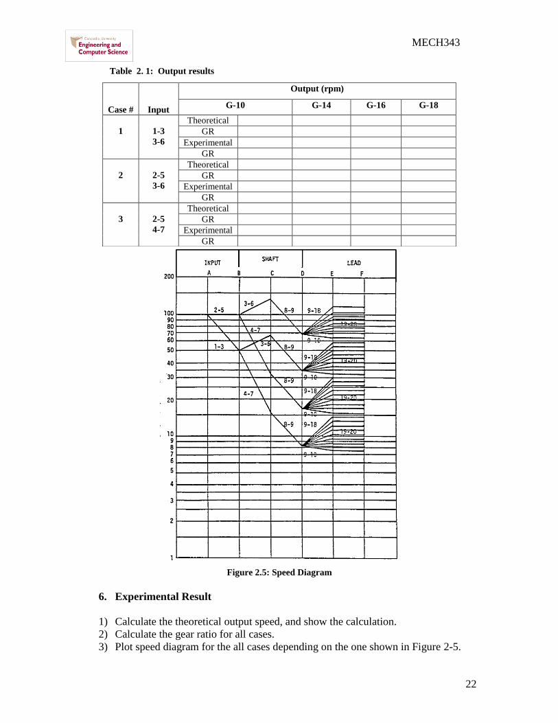
22
MECH343
Table 2 1 Output results
Figure 25 Speed Diagram
6 Experimental Result
1) Calculate the theoretical output speed and show the calculation
2) Calculate the gear ratio for all cases
3) Plot speed diagram for the all cases depending on the one shown in Figure 2-5
Case
Input
Output (rpm)
G-10 G-14 G-16 G-18
1
1-3
3-6
Theoretical
GR
Experimental
GR
2
2-5
3-6
Theoretical
GR
Experimental
GR
3
2-5
4-7
Theoretical
GR
Experimental
GR
23
MECH343
EXPERIMENT 3
Hook (Cardan) Joint or Universal Joint
1 Introduction
The simplest means of transferring motion between non axial shafts is by means of one or
two universal joints also known as Cardan joints in Europe and Hookrsquos joints in Britain
The shafts are not parallel to one another and they may be free to move relative to one
another For this reason this very simple spherical mechanism appears in an enormous
variety of applications The most common application is Cardan joint used in the trucks
as shown in Figure 31 A universal joint is a simple spherical four-bar mechanism that
transfers rotary motion between two shafts whose axes pass through the concurrency
points The joint itself consists of two revolute joints whose axes are orthogonal to one
another They are often configured in a cross-shape member as shown in Figure 32
2 Objective of Universal Joint
Coupling is used to connect two intersecting shafts
Consists of 2 yokes and a cross-link
Figure 31 Cardan Joint used in Trucks
Figure 32 Schematic of Cardan Joint
The transmission behavior of this joint is described by Equation (31)
12 tan
cos
1arctan
(31)
where is the momentary rotation angle of the driven shaft 2
24
MECH343
Figure 33 Schematic of Cardan Joint
The angular velocity ratio can be described by
22
2
4
sinsin1
cos
(32)
where β is the angular misalignment of the shafts and Ө is the angle of the driving shaft
It is noted that
max2
4
at oo 27090
min2
4
at ooo 3601800 (33)
if β = 0 2
4
= 1 = constant at any Ө
2
4
will vary between a minimum and a maximum during each revolution
ω2 = ω4 only at 4 instants as shown in Figure 34
This is a very big disadvantage in case of automotive vehicles this means that rear
wheels will rotate at variable speed
Figure 34 Relation between
2
4
and Ө
ω2 is constant (because engine and flywheel) speed of car cannot be variable each
revolution because its inertia and so this means tires will slip and severe wear will
happen
25
MECH343
The effect of the angle β can be shown by plotting 2
4
for different values of β (Figure
35)
Figure 35 Relation between
2
4
and β
The acceleration expression of the follower of universal joint for constant ω2 is given by
222
22
24
sinsin1
2sinsincos
(34)
Recall y = u(x)v(x) therefore yrsquo= [vursquo-uvrsquo]v2
For acceleration or retardation
-acceleration when 2Ө lies between 0 -180o
-deceleration when 2Ө lies between 180 -360o
Maximum acceleration occurs when dα4 dӨ = 0 Thus
42
2
maxsin2
sin22cos
forgives
(35)
It is possible to connect 2 shafts by 2 Hooks couplings and an intermediate shaft that the
uneven velocity ratio of the first coupling will be cancelled out by the second Condition
(Figure 36)
42 (36)
Yoke 32 lies in plane containing shaft 2 3
Yoke 34 lies in plane containing shaft 3 4
Figure 36 Two shafts by two Hooks couplings and an intermediate shaft
26
MECH343
2 Objective
Testing the affect of changing of the angle between the shaft and universal joint on the
input and output shaft speed and calculate the speed ration between output and input shaft
speed
3 Experimental Procedure
1) Fixing the input shaft angle 2 0o
2) Setting the output shaft angle 154
3) Filter setting cutoff freq 4 Scope setting ch1 500mv ch2 500mv M 50ms run
scope turn on motor After stable fluctuate signal appear on screen stop scope then
turn off motor
4) Check the input and output shaft speed by using Cursor paired We assume that at
0 N4 is min setting paired cursor at this point as t=0 ms Moving cursor along
ch2 signal and record t and N4 by ∆ __ms __v Fill table 3-1 N2 is input shaft
speed It is constant
5) Repeat step 2 setting the output shaft angle 304 Fill table 3-2
6) Plot the graph of velocity ratio during one cycle for both cases Compare with
theoretical plot using equation 32
Table 3 1 Test results of Cardan joint
154
Table 3 2 Test results of Cardan joint 304
(o) 0 45 90 135 180 225 270 315 360
t (ms)
N4(v)
N2(v)
N4N2
(o) 0 45 90 135 180 225 270 315 360
t (ms)
N4(v)
N2(v)
N4N2
27
MECH343
EXPERIMENT 4
Mechanical Oscillator for Measurement of Friction Coefficient
1 Introduction
The mechanical oscillator is an apparatus which allows the experimental
determination of friction coefficient by measuring the period of an oscillating table As
shown in Figure 41 the apparatus consists of two counter rotating wheels upon which is
placed a table of uniform weight
Figure 41 The mechanical oscillator
If the center of gravity of the table is not centered when it is placed on the rotating wheels
then more of its weight will rest upon one wheel than upon the other Consequently the
frictional forces will not be equal and the table will move in the direction of the larger of
the two forces But the inertia of the table will carry it too far past the center point and the
other wheel will exert the larger frictional force Thus the table will oscillate back and
forth at a frequency which depends upon the coefficient of friction
The basic step to find the equation of motion of the system is to construct the Free Body
Diagram of the oscillating table Figures 2(a) 2(b) and 2(c) show this procedure
Summing the forces in the horizontal plane we have
0RRXg
W21 (41)
or
0XL
W2X
g
W
(42)
hence
0XL
g2X
(43)
28
MECH343
Figure 42 procedure of finding the equation of motion
Since the differential equation of motion of free vibration for a one degree of freedom
system is of the form
02 XX n (44)
where n is the natural frequency of the system then
L
g22
n
(45)
But L
gfn
24 222 (46)
where
f = the frequency of the oscillating table in cps
L = the distances between wheel centers in ft
g = gravity constant
hence 2
22f
g
L (47)
The solution of the equation of motion can be written in the form
tBtAX nn cossin (48)
With the initial condition
00 XandXXt O (49)
one gets oXBandA 0 (410)
The response of the oscillating table is therefore
tL
gXX o
212
cos
(411)
29
MECH343
tL
g
L
gXX o
21212
sin2
(412)
tL
g
L
gXX o
212
cos2
(413)
Thus it may be concluded that the response of the oscillating table is governed by the
initial displacement X0 the coefficient of friction micro and the difference between wheel
centers L
2 Objectives
The experiment is designed to illustrate some of the direct applications of the
theory of vibration to the measurement of physical quantities The experiment also
demonstrates the differences between mathematical models and actual physical systems
Calculate the friction coefficient between the wheels and the bars
3 Description of Experiment
The oscillating table apparatus consists of four grooved wheels mounted on two
axels which are driven by a 120 HP electric motor and a gear reduction unit in opposite
directions The table consists of circular rods connected in a rectangular shape such that
the rods are guided by the grooved wheels
4 Experimental Procedure
1) Measure L the length between the centers of the two wheels
2) Locate one of the bars on the wheels
3) Select two different speeds for the wheels and when it starts rotating and the bar
moving calculate the time for 10 oscillations
4) Calculate the experimental coefficient of friction μ through the following
equation 2
22f
g
L When f is the frequency g gravity acceleration L the
length between the centers of the two wheels Fill table 4-1
5) Find the theoretical coefficient of friction μ for all bars
6) Compare between theoretical and experimental coefficient of frictions μ
Table 4 1 Combinations for measuring the friction coefficient
Case Material of
the bar
Speed
(rpm)
Time taken
for 10
oscillation
Frequency
(f)
Coefficient
of friction
(micro)
Standard
coefficient
of friction
1 Steel
2 Brass
3 Aluminum
30
MECH343
EXPERIMENT 5
5-1 PLANETARY GEAR TRAIN KINEMATICS
1 Introduction
A planetary gear train is one in which the axis of some of the gears may have motion A
planetary gear set always includes a sun gear one or more planet gears and a planet
carrier or arm which sometimes called as sun-and-planet planetary gear train as shown in
Figure1
Figure 51 Planetary gear train
A planetary gear set as shown in Figure 52 is one having two degrees of freedom This
means that the motion of each and every element of the mechanism is not defined unless
the motion of two of its elements is specified To make the planetary set a one degree of
freedom gear train one must fix the motion of one element of the mechanism
Figure 52 Sun-and-planet planetary gear train
2 Solution of Planetary Trains by Formula Methods
Figure 53 shows a planetary gear set which is composed of a sun gear 2 an arm 3 and
planet gears 4 and 5
31
MECH343
Figure 53 Compound Planetary Gear Set
We can express the velocity of gear 2 relative to the arm 3 in the form
3223 nnn (51)
3553 nnn (52)
Dividing Equation (52) by (51) gives
32
35
23
53
nn
nn
n
n
(53)
Since this ratio is the same and is proportional to the tooth numbers it is equivalent
therefore to the train value e
32
35
nn
nne
(54)
Or AF
AL
nn
nne
(55)
where nF = rpm of first gear in train
nL = rpm of last gear in train
nA = rpm of arm
The experiment is designed to demonstrate the fundamentals of planetary gear train and
to show all possible motions that can be obtained with this type of gear trains
3 Objective
Calculate the gear train ratio for the planetary gearbox and the degrees of
freedom that the system has
4 Experimental Procedure
For the planetary gear trains mechanism shown in Figure 51
1) Calculate the degree of freedom to the planetary gear system
2) Calculate the gear train ration through the following equation
21
23
nn
nne
When the outer ring is fixed
When the planet gears are fixed
32
MECH343
5-2 The Borg-Warner Model 35 Automatic Transmission
Simulator
1 Introduction
The Borg-Warner Model 35 Automatic Transmission comprises a three element
torque converter--coupling and a planetary gear set to provide three forward ratios and
reverse
The planetary gear set consists of two sun gears two sets of pinions a pinion
carrier and a ring gear
Power enters the gear set via the sun gears In all forward ratios power enters
through the forward sun gear In reverse it enters through the reverse sun gear Power
leaves the gear set by the ring gear and the pinions are used to transmit power from the
sun gears to the ring gear
In reverse a single set of pinions is used which causes the ring gear to rotate in the
opposite direction from the sun gear In forward ratios a double set of pinions is used to
cause the ring gear to rotate in the same direction as the sun gear
The Carrier locates the pinions relative to the two sun gears and the ring gear also
forming a reaction member for certain conditions The various mechanical ratios of the
gear ser are obtained by the engagement of hydraulically operated multi-disc clutches and
brake bands
Power flow in each ratio is achieved by locking various elements of the planetary gear set
as follows
1st Gear (Lockup selected)
The front clutch is applied connecting the converter turbine to the forward sun
gear The rear band is also applied holding the pinion carrier stationary The gear set
provides the reduction of 239 l The reverse sun gear rotates freely in the opposite
direction to the forward sun gear
33
MECH343
1st Gear (Drive selected)
The front clutch is applied connecting the converter turbine to the forward sun
gear The one-way clutch is in operation preventing the pinion carrier from moving
opposite to the engine rotation The gear set again provides the reduction of 239 1 On
the overrun the one-way clutch unlocks and the gear set freewheels
2nd Gear (Lockup or drive selected)
Again the front clutch is applied connecting the converter turbine to the forward
sun gear The front band is applied holding the reverse sun gear stationary The pinions
now walk around the stationary sun gear and the gear set provides the reduction of 145
l
3rd Gear (Drive selected)
Again the front clutch is applied connecting the converter turbine to the forward
sun gear The rear clutch is applied connecting the turbine also to the reverse sun gear
Thus both sun gears are locked together and the gear set rotates as a unit providing a
ratio of 1 1
Neutral and Park
The front and rear clutches are released and no power is transmitted from the
converter to the gear set
Reverse
The rear clutch is applied connecting the converter turbine to the reverse sun gear
The rear band is applied holding the pinion carrier stationary providing a reduction of
209 l
2 Gear Ratios
119866119890119886119903 119877119886119905119894119900 120579119900120579119894
=1
239
The carrier is held stationary to provide the
reaction member and the gears operate as a
Simple gear train
34
MECH343
The reverse sun gear is held to that the gears
now operate as an epicyclic gear train
For an epicyclic gear train shown as following
119866119890119886119903 119877119886119905119894119900 120579119900120579119894
=1
145
119894134 =
1205961 minus 1205964
1205963 minus 1205964= minus
11988521198851
11988531198852prime
119900119903 120596119871
32
67= 120596119869 minus 120596119871 120596119869 =
99
67120596119871
For our transmission show as above
119894119865119869119871 =
120596119865minus120596119871
120596119869minus120596119871= minus
119885119866
119885119865
119885119867
119885119866
119885119869
119885119867=
67
28 (1)
119894119865119870119871 =
120596119865minus120596119871
120596119870minus120596119871= minus
119885119866
119885119865
119885119867
119885119866
119885119870
119885119867= minus
32
28 (2)
Hence minus120596119871
120596119869minus120596119871= minus
67
68
28
32
From (2) 120596119865 minus 120596119871 =32
28 120596119871 120596119865 =
60
28120596119871
Therefore 119894119865119869 =120596119865
120596119869=
60
28
67
99= 145021645
So 120579119900
120579119894=
1
145
35
MECH343
119866119890119886119903 119877119886119905119894119900 120579119900120579119894
=1
1
Both sun gears are locked together and the
gears set rotates as a unit
119866119890119886119903 119877119886119905119894119900 120579119900120579119894
=1
209
With the reverse gear engaged power is
applied to the reverse sun gear The planet
carrier is held stationary so that the planet
gears rotate the ring gear in the opposite
direction to the reverse sun gear
36
MECH343
3 Experimental Procedure
Pins and slotted plates represent the multi-disc clutches and brake bands The various
gear ratios of the gear set may be obtained by inserting the appropriate pins as indicated
below
A B C D E F
Lockup 1Drive 1
Lockup 2Drive 2
Drive 3
Reverse
Neutral
Park Note
1 Lose all pin and turn input shaft and output shaft make sure input shaft disk and
output shaft disk indicate to 0 then lock pins for each case
2 Turn input shaft one turn (360 ) read output disk (degree)
3 Fill out following table
Input (degree) Output (degree)
Lockup 1Drive 1 360
Lockup 2Drive 2 360
Drive 3 360
Reverse 360
4 Results
According to power flow and gear ratio figures for each case referring to 2nd gear
ratio calculation derive and calculate gear ratios for 1st 3
rd and reverse shift Compare
them with your experimental results
37
MECH343
EXPERIMENT 6
Static and Dynamic Balancing
1 Objective
The objectives of this experiment are
Understanding the concept of static and dynamic balancing
Understanding unbalance torque
Justifying theoretical calculation for balancing with experiment
Balancing the shaft by the four given masses
2 Introduction
Unbalanced dynamic forces effects have profound influence on the working and
of rotating machinery like turbines compressors pumps motors etc These forces act
directly on the bearings supporting the rotor and thus increase the loads and accelerate the
fatigue failure These unbalanced forces induce further mechanical vibrations in the
machinery and connected parts thereby creating environmental noise problem through
radiation of sound Hence it is desirable to balance all such uncompensated masses and
thus reduce the effect of unbalance forces in a dynamics balancing machine
Balancing is the technique of correcting or eliminating unwanted inertia forces which
cause vibrations which at high speeds may reach a dangerous level An important
requirement of all rotating machinery parts is that the rotation axis coincides with one of
the principal axis of inertia of the body After a roll is manufactured it must be balanced
to satisfy this requirement especially for high speed machines The condition of
unbalance of a rotating body may be classified as static or dynamic unbalance
2 1 Static Unbalance
An idler roll is statically balanced if the roll doesnt rotate to a heavy side when free to
turn on its bearings Thus the rolls center of gravity is on the axis of rotation Static
unbalance (Figure 61) creates a centrifugal force when rotating which causes deflection
of the roll Idler rolls are sometimes static
balanced only when the roll operates at slow
speeds
The static unbalance usually happens because
of errors in the manufacturing tolerances of
the rotating parts Therefore static imbalance
is essentially a weighing process in which the
part is acted upon by either gravitational or
centrifugal force This type of unbalance
could be easily reduced or removed by static
balancing
Figure 61 Static (or force) Unbalance
38
MECH343
2 2 Dynamic Unbalance
An idler roll may be in perfect static balance and not be in a balanced state when rotating
at high speeds A dynamic unbalance is a ldquocouplerdquo or twisting force in two separate
planes 180 degrees opposite each other (Figure 62) Because these forces are in
separate planes they cause a rocking motion from end to end A roll that is unbalanced
will cause 1) machinery vibrations 2) web
flutter and 3) a decrease in bearing life due to
unnecessary forces
To dynamically balance a roll it must first be
statically balanced Then the roll must be
rotated to its operating speed and have the
dynamic unbalance eliminated by adding or
subtracting weight The determination of the
magnitude and angular position of the
unbalance is the task of the balancing
machine and its operator Balancing
machines are provided with elastically
supported bearings in which the idler roll may
spin Because of the unbalance the bearings
will oscillate laterally and the amplitude and
phase of the roll are indicated by electrical
pickups and a strobe light
Figure 63 shows a long rotor which is to be mounted in bearing A and B We might
suppose that two equal masses m1 and m2 are placed at opposite ends of the rotor and at
equal distances r1 and r2 from the axis of rotation Since masses are equal on opposite
sides of the rotational axis the rotor is statically balanced in all angular positions But if
the rotor is caused to rotate at an angular velocity ω radsec the centrifugal forces m1r1ω2
and m2r2ω2 act respectively at m1 and m2 on the rotor ends These centrifugal forces
produce the equal but opposite bearing reactions FA and FB and the entire system of
forces rotate with the rotor at the angular velocity ω Thus the rotor is to be statically
balanced and at the same time dynamically unbalanced
Figure 63 Dynamically Unbalanced Rotor
Figure 62 Dynamic (or couple) Unbalance
39
MECH343
3 Principle and Theory of Operation
Consider a body of mass M rotating with a uniform angular velocity about O with
eccentricity e as shown in Figure 64 The centrifugal force Fc acting on the axis of
rotation is Me2 This force is therefore very sensitive to speed and hence there is a need
to reduce this force either by operating at lower speeds or by decreasing the eccentricity
as shown in Figure 65
O
e
M
M e
2
Figure 64 Unbalanced Disc
Center of rotation
( new center of
gravity )
Rotating Disc Added mass m
Center of gravityOriginal center
of gravity
(a) (b)
Figure 65 Illustration of The Simplest Method of Static Balancing
In general it is desirable to make e as low as possible If the rotor thickness to diameter
ratio is less than 05 and speed are below 1000 rpm the rotor can be single plane
balanced - otherwise two-plane balancing is necessary In the single plane balancing
technique with a rotor of mass mi and radius ri from the axis of rotation and lying in the
same plane the condition for static balance is used
0~iirm (61)
where i = 1 2 which denotes the total number of masses and m denotes the mass The
vector ir~ represents the eccentricity e of the mass mi from the axis of rotation
When the bodies are rotating in several planes the condition for dynamic balance has to
be satisfied in addition to that for static balance This is given by
0~~ iii rzm (62)
where iz~ is the axial coordinate vector of the mass mi measured for a chosen datum In
the two-plane balancing technique instead of satisfying Equations (61) and (62)
40
MECH343
explicitly Equation (62) is used with two different datum planes for iz~ Mathematically
if the distance between these two plane is oz~ then
0~)~~( ioii rzzm (63)
It is therefore clear that Equations (62) and (63) imply the satisfaction of Equation
(61) Conceptually it means that if a system of bodies rotating in several planes is in
dynamic balance with respect to two different datum planes then the system is also in
static balance This is the principle of the two-plane balancing technique
4 Description of Experimental Apparatus
Figure 66 shows the Static and Dynamic Balancing Apparatus It consists of a perfectly
balanced shaft with four rectangular blocks clamped to it The shaft is mounted in ball
bearings and it is driven by a 12 volt electric motor through a belt and pulley drive The
shaft assembly is mounted on a metal plate resting on four resilient rubber supports
which allow the mount to vibrate when the shaft is not balanced
The rectangular blocks can be clamped to the shaft at desired out-of-balance moments by
means of discs having eccentric holes of various diameters The discs are fixed to the
blocks by hexagon socket set screws Any longitudinal and angular position of a block
relative to the shaft can be set by linear and protractor scales provided Adjacent to the
linear scale is a slider which can be pushed against the block to read its longitudinal
position The slider also serves as a datum stop against which the blocks can be held
when reading their angular position on the shaft
The out-of-balance moments are measured by fitting the extension shaft and pulley to the
main shaft Each rectangular block is then clamped to the shaft in succession A cord with
a weight bucket at each end is hung on the pulley and bearing balls are placed in the
bucket until the block has turned through 90deg The out-of-balance moment is proportional
to the number of balls required
to turn the block
A Perspex dome serves as the
safety cover The shaft cannot
be driven unless the dome is in
position which is achieved by
micro switches actuated by the
dome The motor switch on the
front panel is spring loaded so
that the motor cannot be left
running The motor requires a
power supply of 12 volts at 2
amperes which is provided by
E66E90 speed controller
Figure 66 Static and Dynamic Balancing Apparatus
41
MECH343
5 Experimental Procedure
5 1 TEST 1 Static Balancing
1 Looking at the shaft from the side the masses will be as shown in figure 6-7
each mass has an angle θ with horizontal
Figure 6-7 Shaft view from the side
2 The masses forces are given by the following table 6-1
The masses values Table 6-1
3 In order to balance the shaft statically the sum of the forces will be equal zero
as the following equations
sum F=0
F1cos θ1+ F2cos θ2+ F3cos θ3+ F4cos θ4=0 (1)
F1sin θ1+ F2 sin θ2+ F3 sin θ3+ F4 sin θ4=0 (2)
4 Since we have just two equations with four unknown angles we assume
θ1=0ordm θ2=90ordm
5 Solving the two equations or using force polygon by AutoCAD to find the θ3
θ4
5 2 TEST 2 Dynamic balancing
1 Looking for the shaft from in front the masses create the forces as shown in
figure 6-8 each mass has an arm X create a momentum
F1
F2
F3
F4
42
MECH343
2 In order to balance the shaft dynamically the sum of the momentum will be
equal zero as the following equations
sum M=0
F1cos θ1X1+ F2cos θ2X2+ F3cos θ3X3+ F4cos θ4X4=0 (1)
F1sin θ1X1+ F2 sin θ2X2+ F3 sin θ3X3+ F4 sin θ4X4=0 (2)
3 Since we have just two equations with four unknown arms we assume
X1=50 mm X2=100 mm
4 Solving the two equations or using momentum polygon by AutoCAD to find
the X3 X 4
TABLE 6 2
Block 1 2 3 4
Mass 88 82 74 64
Angle θ(ordm) 0 90
Arm X (mm) 50 100
6 Typical Calculations
The basic equations that are used for balancing purposes are
0rW ii (63)
0rWa iii (64)
Suppose that block (1) is placed 17 mm from the left end of the shaft at zero angular displacement and that
block (2) is placed 100 mm from it at 120deg The measured out-of-balance moments are as follows
Figure 68 In front shaft view
43
MECH343
TABLE 6 3 OUT-OF-BALANCE MOMENTS
It is first necessary to draw the moment polygon of Wr values as shown in Figure 68 to determine the
angular positions of blocks (3) and (4) W1r1 and W2r2 are known in both magnitude and direction The
vector W1r1 has been drawn at positive X-direction (θ = 0) The lengths of vectors W3r3 and W4r4 are known
and arcs can be drawn from the ends of W1r1 and W2r2 to get the directions of the unknown vectors
Figure 69 shows the diagram of the angular positions and the corresponding longitudinal locations of the
blocks on the shaft are 17 mm for the first 117 mm for the second block
To find the longitudinal positions of the other two blocks we designate distance of block (3) by a3 and
distance of block (4) by a4 measured from block (1) so block (1) is the reference and will not appear in
calculations
Draw a vector a2W2r2 = 100 (82) units long parallel to r2 and vectors a3W3r3 and a4W4r4 parallel to r3 and r4
respectively so that the moment polygon is closed The lengths of vectors a3W3r3 and a4W4r4 can be
measured and the magnitudes found by using the scale factor From these a3 and a4 can be calculated
Notice that the sense of vector a3W3r3 is reverse In order to maintain vector a3W3r3 the only possible
solution is to reverse a3 So from the vector polygon (triangle) it follows
a3 = -12 mm
a4 = 124 mm
This means that block (3) should be located 5 mm from the left end of the shaft The blocks should be
positioned as follows
Block Angular Position (Deg) Longitudinal Position (mm)
(1) 0 17
(2) 120 117
(3) 190 5
(4) 294 141
The values of a3 and a4 can be found analytically using complex vector approach
Real and imaginary components yield
100(82) cos 120deg + (74) a3 cos 190deg + (64) a4 cos 294deg = 0
100(82) sin 120deg + (74) a3 sin 190deg + (64) a4 sin 294 deg = 0
which reduce to
4100- 7288 a3 -2603 a4 = 0
71014- 1285a3 -5847 a4 = 0
44
MECH343
Solving the two equations gives a3 = -1194mm a4 = 12396mm
The values compare very well with those obtained graphically
In order to obtain independent results it is suggested that Wr values of the blocks are varied by using
different positions of the discs with eccentric holes The angular displacements between blocks (1) and (2)
may also be varied
Figure 69 Moment Polygon of Wr
45
MECH343
EXPERIMENT 7
Machine Fault Simulator (MFS)
1 Theory
Refer to experiment number 6
2 Description of Experimental Apparatus
Figure 71 shows the machine fault simulator The rotor is driven by a variable speed
motor via a flat belt and the rotor rotational speed is captured through a digital
tachometer The vibration due to the unbalanced rotor is measured and fed directly into
the on-board processor of the machine
Figure 71 Machine Fault Simulator
3 Objective
In this experiment we will study the reaction of the shaft and the motor when the shaft is
balanced and when it is unbalanced
4 Experimental Procedure
1) Run the Vibro-Quest Software
o Define a ldquoNew Projectrdquo (under root)
o Fill up the window select ldquoProject namerdquo click ldquoNextrdquo
o Select ldquoNonerdquo from the menu on the right side click ldquoNextrdquo
Belt
Motor
Disk A Disk B
Reciprocating
Mechanism
Speed
Control
46
MECH343
o Review the table (do not change the default) click ldquoNextrdquo
o Review the table check the setting data click ldquoNextrdquo
o Click ldquoDonerdquo
o Review the information provided if they are not ok ldquoGo backrdquo to modify
the data then click ldquoFinishrdquo
2 Select ldquoDatardquo from the toll bar on the computer
3 Name the ldquoTest Titlerdquo in the window Insert the parameters used in the test and
click ldquoNextrdquo
4 Review the information provided in the window and click ldquoNextrdquo
5 Chose 2000 as Frequency limit 1600 for Space line Leave the rest information as
defaulted and ldquoGO DAQrdquo
2) Running the Machine Fault Simulator
Select the required speed (rpm) change it to frequency (Hz) using the following
relation 60)rpm(n2)Hz(f
1 Run the machine using speed control system at desired speed
2 Wait about 15 seconds to stable the system
3 Click onrdquo START RECORDINGrdquo
4 When the recording is finished save the file under the root of ldquoDatardquo of base line
at the subdirectory that you want to compare with the other data (for example if
you are running the machine at 20 Hz save the your file under 20 Hz subdirectory)
5 Now select the ldquoProject namerdquo from the left menu all the relevant tests will
appear at the right table under the ldquoTest Explorerrdquo
6 To compare the data from different files Hold down the ldquoShiftrdquo key and select
any two interested files that you are going to compare
7 Click on ldquoComparerdquo to observe the difference between the unbalanced system
with a base system
8 To observe more clearly the difference between the frequency responses of the
different test click on ldquoOverlayrdquo
TEST 1 Imbalance Effects on Vibration response
Install the defined weight in one of the taped hole in rotor disk A and tight it
securely with a nut
Close the cover of MFS
Change the motor speed and record vibration level at each bearing For this
purpose you don not need to define new project for each speed define a new
project( follow steps 1-6 from section 3) then follow steps 1-2 for each speed
from section 4
Measure the average level of amplitude at each speed and Plot it against the speed
Repeat steps 2-5 for 2 different weights at 2 different radius and angles
47
MECH343
TEST 2 Balancing the Imbalance Rotor
Add weight at different radius and angles using the ldquosample calculationrdquo to
balance the rotor
If the rotor is balanced define a ldquoNew projectrdquo and follow steps 3-8 of Section 4
Fill Table 7 1
TABLE 7 1
Unbalance weight on disc A ____________ angular position _______________
Mass Added on disk B gr r (mm)
Amp baseAmp New
48
MECH343
EXPERIMENT 8
DETERMINATION OF SPUR GEAR EFFICIENCY
1 Objective
The main objective of the experiment is to determine the efficiency of the
Spur gear and worm gear unit
2 Introduction and theoretical background
21 Pinion gear
Two intermeshed toothed wheels make up a pinion gear This type of gear
permits a positive transmission of motion and torque Wheel pairs are available in
different shapes and shaft configurations Figure 1 explains the various types of gears and
their arrangements
Fig8 1 Various types of gear arrangements
22 Worm gear
A worm gear is a screw-type transmission unit whose axes generally intersect at
right angles The worm and wheel make contact on a straight line Normally the worm
has a cylindrical core and the wheel globoid toothing Units with a very high performance
49
MECH343
consist of a globoid worm and globoid wheel A worm gear with a cylindrical worm has
the following special features
High load capacity compared with spur gears due to linear contact
Low-noise operation and high absorption of vibrations
Wide transmission range down to low ilt110
High efficiency at high transmission ratios high efficiencies(η le 98 ) can be
achieved with very sophisticated designs under favorable operating conditions a
decrease in pitch angle (high transmission ratio) or speed is accompanied by a
corresponding decrease in efficiency (to η le 50 )
Self-locking operation
Smaller and lighter design compared with spur bevel gear units possessing high
transmission ratios
23 Basic definitions
Drive torque
The drive torque is the product of the force F and the lever arm l on which the
force acts
M = F X l (1)
M is in Nm F is in N and l in m
Drive power
The drive power of a rotating shaft is the product of the torque M and angular
frequency ω P = M X ω (2)
and 60
2 n (3)
P is in W n is in rpm
Efficiency
The efficiency is defined as the ratio between the output and input powers It has a
maximum theoretical value of 1
in
out
P
P (4)
where speed i
nn 1
2
50
MECH343
3 Experimental set-up
Figure 2 shows the complete view of the experimental set up
Fig8 2 Complete view of GUNT AT 200 experimental set up
The modules comprising the drive unit spur gear worm gear and magnetic
powder brake are mounted on a profile frame The DC shunt motor is designed for right-
hand and left-hand rotation The drive unit is electrically powered via control housing
The control unit adjusts the DC machinersquos speed via its armature voltage Its target speed
is set by means of a potentiometer on this housing Its actual speed is measured and
indicated by means of an inductive proximity switch and evaluation unit The speed is
51
MECH343
measured inductively by a contactless sensor disc and indicated by a digital display
element on the control unit Electronic thyristor speed control with I x R compensation
provides a high torsional rigidity The reaction torque exerted on the drive housing is
measured by means of a spring force meter connected to a lever arm
The transmission units consist of a 2-stage spur gear with transmission
ratio i = 135 and a single-stage worm gear with transmission ratio i = 14The
transmission torque can be determined on the drive side as well as the brake side To
facilitate adjustment of the brake torque the brake characteristic (current torque) is
recorded in a preliminary experiment Moments are determined through power
measurements (spring balance) with a known lever arm The moments measured input
speeds and transmission ratios are used to determine power and efficiency
The magnetic powder coupling consists of two independently mounted
rotors ie a primary and a secondary rotor both furnished with ball bearings The
primary rotor also serves as a coil carrier If one of these two rotors is deactivated the
magnetic powder coupling can also be used as a brake The air gap between the two
rotors contains a special magnetic powder If a direct voltage is applied to the excitation
winding the powder aligns itself with the resulting magnetic field lines to form a
compact mass providing a frictional link between the primary and secondary rotors The
value of the torque depends on the adjusted current When the current-proportional
moment is exceeded slippage occurs without any transition
4 Experiments procedure
As shown in Figure 82 the complete view of the experimental set up for this
experiment there is input as the motor speed and the output as excitation current so that
there is two steps for this experiment
After making sure spur gear is connected as shown in Figure 83
1) Fix the output excitation current at I= 50 mA and change the speed of the motor as
shown in the table (1) each time measure the motor force F1 and the brake force F2
52
MECH343
Figure 83 Configuration of spur gear unit experimental set up
Measurement data to determine the efficiency of Spur gear unit Table (1) I = 50mA
SlNo Motor speed
( n1 ) rpm
Motor holding
force ( F1 ) N
Brake holding force
( F2 ) N
Efficiency ( η )
1 500
2 1000
3 1500
4 2000
5 2500
In order to find out the spur gear efficiency we go through the following equations
The general equation for the spur gear efficiency is
in
out
P
P
The drive power of a rotating shaft is the product of the torque M and angular
frequency ω P = M X ω
The drive torque is the product of the force F and the lever arm l on which the
force acts
M = F Arm
When the arm for the motor Arm1=25 mm and for the brake Arm2=50 mm
53
MECH343
And the angular velocity from the following equation
60
2 n
In order to find the speed for the brake we use this ratio assuming i= 135
i
nn 1
2
2) Fixing the input n1= 1500 rpm and changing the output and filling table (2)
Recorded values of the excitation current and the force on the lever arm table (2)
Speed n1= 1500 rpm
Excitation current I (mA) Force F2 on the lever arm (N)
50
70
90
110
130
150
130
110
90
70
50
5 Experiments Results
1) Plot the characteristics curve between the current I and the force on the lever arm
F2
2) Plot the characteristics curve between the current I and the torque M
3) Determine the efficiency of the spur gear unit Comment on the errors on the
efficiency if the calculated efficiency deviates from the realistic values of 80 -
90
54
MECH343
EXPERIMENT 9
ANALYSIS OF LINKAGE MECHANISM
Try to build a linkage mechanism as the figure below
Steps
1 Turn on grid line from View-workspace-grid lines as below
2 Select rectangle tool
55
MECH343
3 Click and drag a small rectangle
4 Click the rectangle copy it (CTRL+C) paste it (CTRL+V) two times
5 Change the length of each rectangle by selecting it and writing down the desired
length in the text box named W
Make the length as (3 ndash 332 - 4)
56
MECH343
6 Use the rotate tool and the select tool to arrange the rectangles
Make sure that the spacing is 4 units as shown below
7 Put a motor at the lower end of the left link
- First select the motor - Then click at the desired point
57
MECH343
8 Put a pin joint at the lower end of the right link
- First select the pin joint - Then click at the desired point
9 Put a point element at the remaining ends
- First double click (this
enable you to assign multiple
points) on the point element
It should look like below
58
MECH343
10 Join the links by selecting two points then selecting Join
Click the arrow select tool
Select first point ndash
press SHIFT and
click the other point
Press
Join
They should look like
below
11 Repeat the same for the remaining two points Your model should look like below
59
MECH343
12 Click RUN ( ) and watch it rotating
13 Now we want to capture the velocity of the joint between the left link and the middle
one
- Select it and click on Define ndash Vectors-
Velocity
Click Run and watch the velocity change
Note that by clicking on the link itself and defining the velocity the program calculates
the velocity of the CG of the link
14 Now you are ready to try different measurements
Acceleration Total Force Gravitational Force
60
MECH343
15 Select a link and use the measure tool
X- Position Graph
Y- Position Graph
61
MECH343
Measuring velocity values
16 Now try to change the length of any of the links and RUN the model and observe
for any change if any and explain
17 Change the mass of any of the links and observe for any change in velocity and
force And Why if there is any
18 Now double click on the motor (resetting the mass for any link that has been
changed) and notice that the value for velocity is 1 radsec Change this to make it the
same value for acceleration and torque Write what you observe and try to explain
19 Now increase the mass for one link (eg left one) gradual and see how this will
affect the motion for a fixed value for torque velocity or acceleration of the motor
20 Now replace the middle link with two links connected with total length as the
middle one run observe and explain
21 Based on (20) search for what is the equation relation or rule that governs the
mechanism motion
62
MECH343
EXPERIMENT 10
NUMERICAL DYNAMIC SIMULATION FLYWHEEL
Problem Definition
In the two cycle piston engine shown explosive gases are
ignited in the combustion chamber above the piston The
explosions apply a force of 150 N for the duration of every
downward stroke The engine is equipped with a speed
limiting device (rev limiter) which prevents the rotational
speed from exceeding a set value (red-line) The masses of
the piston and connecting rod are 075 kg and 15 kg
respectively The mass of the crankshaft-flywheel assembly
is 30 kg Given that the red-line of the engine is 35 radsec
(340 rpm) Assume the crankshaft-flywheel assembly can
be modeled as a circular disk
Objective
Determine the forces at the crankshaft bearing (point A) and connection rod (point B)
bearing
Solution
1 INTRODUCTION
Engines that exceed the manufacturers maximum speed (over-revving) may be subject to
excessive wear and possible failure To prevent over revving internal combustion
engines are often fitted with a device known as a rev-limiter When an engine exceeds its
red-line rev-limiters interrupt the ignition system slowing the engine down Once the
speed drops below the maximum the ignition system is switched back on In this exercise
you will model an internal combustion engine equipped with a rev-limiter The engine
has three bodies the piston the connecting rod and the crankshaft The piston will be
modeled by a square body The connecting rod will be modeled by a rectangular body
The crankshaft will be modeled as a circular body The bodies will be drawn sized and
joined to each other and the background The pistons cylinder walls will be modeled with
a keyed slot joint The force of combustion will be modeled by a force attached to the top
of the piston The resulting forces at the bearings will be measured
2 SETTING UP THE WORKSPACE
For this exercise three changes in the workspace will be made First for clarity the x-y
axes will be displayed The unit of distance will also be changed from meters (default) to
millimeters
63
MECH343
If the x-y axes are not currently displayed choose Workspace from the
View menu and choose XY Axes from the Workspace submenu The x-y
axes provide a reference frame for building a simulation
Choose Numbers and Unitshellip from the View menu The Numbers and
Units dialog appears
Click the More Choices button The dialog box expands
Click and hold in the Distance field (Figure 1) The pop-up menu appears
Choose millimeters from the Distance pop-up menu
Click in the Rotation field and choose Radians from the pop-up menu
Click OK
3 CREATING THE COMPONENTS
This exercise has three objects a 15 kg connecting rod a 075 kg piston and a 30 kg
crankshaft (see Figure 2 below) The connecting rod will be modeled by a thin rectangle
400 mm in length Its width will be thin 150 mm so it closely resembles the actual
connecting rod The crankshaft as stated in the exercise is modeled as a circular disk
with a 200 mm radius and a mass of 30 kg A 200 mm square object will represent the
piston The objects will be created sized and initialized in the following steps
Creating the Crankshaft
The crankshaft is represented by a circle with a radius of 200 mm and mass of 30 kg
These parameters will be set using the Geometry and Properties utility windows
I To draw the crankshaft
64
MECH343
bull Click the Circle tool in the Toolbar
bull Click once on the background Move the mouse to expand the circle and click
again to complete sketching
II To set the mass of the crankshaft
Choose Properties from the Window menu
Click the mass field and enter the value 30
III To set the size of the crankshaft
Select the crankshaft if it not already selected
Click the Radius field (labeled ldquorrdquo) of the Coordinates bar and enter the value 200
(Figure 3)
IV Zooming In
The circle will appear small after sizing To make the rectangle easier to manipulate and
appear larger the workspace will be magnified using the Zoom tool To zoom in
Click the Zoom In tool in the Toolbar
Click near the circle The objects in the window are magnified by a factor of two with
each click of the mouse To zoom out while the Zoom In tool is selected hold down
65
MECH343
the Shift key (the magnifying glass pointer changes to ldquo-rdquo) and click Your screen
should be similar to Figure 4 below
Figure 4 The workspace after zooming in
Click the Arrow tool in the Toolbar or press the spacebar to deselect the Zoom In
tool
Creating the Piston
For this exercise the piston will be modeled as a 200 mm square with the mass of 75 kg
The Square tool will be used to draw the piston and the Properties window will be used
to set its mass
I To draw the piston
Choose the Square tool in the Toolbar On systems the Square tool is ldquohiddenrdquo in the
RectangleSquare pop-up palette by default Click and hold on the Rectangle tool to
bring the pop-up palette in view (Figure 5 below)
Click once on the background drag to the right and click again to complete
sketching A square appears on the screen To set the size of the piston
Click in the Height or Width field of the Coordinates bar and enter 200 Either field
changes both the height and the width of the object so that it remains square
Figure 5 RectangleSquare pop-up palette
II To set the pistonrsquos mass
bull Select the piston if it not already selected
bull Choose Properties from the Window menu
66
MECH343
bull Click in the mass field and enter the value 075
Creating the Connecting Rod
In this exercise the connecting rod is represented by a rectangle drawn with the
Rectangle tool and sized using the Geometry window To approximate an actual
connecting rod the rectangle will be given a mass of 2 kg a height of 500 mm and a
width of 100 mm
To draw the connecting rod
I Choose the Rectangle tool in the Toolbar (On systems the Square tool used above
may have replaced the Rectangle tool in the Toolbar If so the Rectangle tool may be
selected from the hidden pop-up palette by clicking and holding on the Square tool in
the Toolbar)
II Click once on the background drag to the right and click again to complete
sketching A rectangle appears on the screen To set the mass of the connecting rod
bull Select the new rectangle if it not already selected
bull Choose Properties from the Window menu
bull Click in the Mass field and enter the value 2
To set the size of the rod
1 Click the Height field of the Coordinates bar and enter the value 500
2 Click the Width field of the Coordinates bar and enter the value 100 Your screen
should resemble Figure 6
Figure 6 The piston crankshaft and connecting rod
Creating the Points for Joining
The objects in this exercise are connected to each other and to the background (see Figure
7 below) The connections will be modeled by creating points and joining them These
points will be created with the Point tool and accurately positioned using the Properties
window
67
MECH343
Figure 7 The points which will be created and their coordinates
Creating Points on the Connecting Rod
Double-click the Point tool in the Toolbar Double-clicking selects a tool for
successive operations On systems the difference between single and double-clicking
is indicated in the Toolbar by shading a doubleclicked item is dark grey while a
single-clicked item is light grey
Place the mouse pointer over the connecting rod rectangle Find the snap point at the
top end of the connecting rod An X symbol appears at snap points Find the snap
point located at the midpoint of the top side of the connecting rod
To attach a point element click when the snap point located at the top end is visible
Observe that the point element is attached to the top end of the rod
In the same fashion attach another point element to the bottom end of the connecting
rod Your screen should resemble Figure 8
Figure 8 Connecting rod points in position
68
MECH343
Attaching Points to the Crankshaft
The crankshaft needs two points a center point representing the main bearing and an
outer point representing the connecting rod bearing These points will be accurately
positioned at the center and at 200 mm from the center of the circle To create and
position the crankshaft points
Make sure the Point tool is still selected Place the mouse pointer over the
crankshaft Find the snap point at the center of the circle
Click when the snap point at the center is visible A point element is attached to
the center of the circle
Place the mouse pointer near the left quadrant of the circle Find the snap point at
the left quadrant (Figure 9) As the mouse pointer nears the left quadrant of the
circle the snap point appears
Click when the snap point at the left quadrant is visible Another point element is
attached to the left quadrant of the circle
Figure 9 Snap point at the left quadrant of the circle
Attaching Points to the Piston
Two points need to be attached to the piston a square point and a point The square point
will be joined to the slot on the background to create a keyed slot joint The point will be
joined to another point on the connecting rod to form a pin joint The square point will be
positioned on the piston at the coordinates of (0 -50) The square point will be rotated 90deg
so that when joined to the slot the piston will not rotate This is because vertical slots are
defined as being rotated 90deg horizontal slots are defined as having 0deg rotation When a
square point is joined to a slot the rotations of the two objects are aligned
I The point will be positioned at (0 0) To create the points
Click the Square Point tool The cursor turns into a square point
Click anywhere on the piston Since the square point will be precisely position
using the Coordinates bar below it is not necessary to find a snap point
Click in the X field of the Coordinates bar and enter 0 If you attached the square
point on a snap point the x-field of the Coordinates bar may contain a formula
expression (such as body[3] width or (00)) Simply overwrite the entire
expression and enter 0
Press the tab key to move to the Y field of the Coordinates bar and enter -50
Again simply overwrite the y-field with the value -50
Choose the Properties in the Window menu The Properties window appears
In the angle field of the Properties window (marked by oslash) enter the value 1571
The value of 1571 radians is equivalent to 90deg The value will be displayed in a
69
MECH343
rounded form but internally the correct value will be used The pointrsquos y-position
is set to -50 so it will not interfere with the connecting rod joint
II To create the point
Click the Point tool
Place the pointer near the center of the square and find the snap point
Click when the snap point at the center is visible The point is created at the center
of the piston
Attaching a Point to the Background
A point representing the main bearing of the crankshaft must be placed on the
background The point can be placed anywhere on the background for clarity it will be
placed at the origin (0 0) To create and position the point
Click the Point tool
Place the mouse pointer near the origin Find the snap point that appears at the
origin Make sure that nobody is obstructing the origin The snap point does not
appear if the origin is covered by a body
Click when the snap point at the origin is visible Verify the position of the point
by noting the (x y) position in the Coordinates bar it should be (0 0) We now
name this point element so that it becomes easier to select later
Choose Appearance from the Window menu The Appearance window appears
In the name field (where it says Point) type Base Pin Since we will not be
needing the Appearance window for the rest of the exercise close the window by
(Windows) clicking the box marked ldquoXrdquo at the top-right corner of the window or
() clicking the box at the top-left corner of the window
Attaching a Slot to the Background
The cylinder walls of the engine will be modeled with a keyed slot joint The joint will be
made by joining the square point on the piston to a slot attached to the background The
slot can be located anywhere on the background as long as it is located on the
crankshaftrsquos centerline (the yaxis for this model)
To create and position the slot on the background
Choose the Vertical Slot tool in the Toolbar On systems the Vertical Slot tool
may be ldquohiddenrdquo in the Slot pop-up palette Click and hold on the Slot tool in the
Toolbar to bring the pop-up palette in view
Place the pointer near the point element attached to the origin Find the snap
point
Click when the snap point is visible A vertical slot appears
Creating Joints
In this exercise there are four joints (see Figure 10) The joints will connect the piston to
the slot the piston to the connecting rod the connecting rod to the crankshaft and the
crankshaft to the main bearing
70
MECH343
Figure 10 The points which will be joined
The following steps will demonstrate how to make these joints
I Joining the Piston to the Slot
In this example the piston slides in a cylinder The
cylinder will be modeled as a keyed slot joint The joint
is created by joining the square point on the piston to the
slot To create the keyed slot joint
Select the square point on the piston and while
holding down the Shift key select the slot The word
ldquoJoinrdquo of the Join button in the Toolbar changes
from gray to black indicating the two points can be
joined
Click the Join button in the Toolbar The piston
moves to the slot (see Figure 11) Joining the
Crankshaft to the Point on the Background The
crankshaft main bearing is modeled as a pin joint
The pin joint will be created by joining the point at
the center of the circle to the point at the origin
II To join the crankshaft to the origin
Choose Properties in the Window menu
From the selection pop-up menu located at the top of the
Properties window choose Base Pin (Figure 12) The
Base Pin is now selected
Hold the Shift key down and select the center point on
the crankshaft circle
Click the Join button The crankshaft circle moves to the
origin
To see how the circle representing the crankshaft is
constrained bring the mouse pointer over the circle hold
down the mouse button and drag the circle The circle
can rotate but is fixed to the Base Pin
Figure 11 Piston joined to the slot
Figure 12 Selecting an object in
the Properties window
71
MECH343
III Joining the Components
The piston connecting rod and crankshaft will now be joined together (see Figure
13) The following steps describe how to join them
Figure 13 Joining the components
IV To join the piston to the connecting rod
Select the (round) point on the piston and while holding
the Shift key down select the top point on the
connecting rod
Click the Join button The two objects will come
together
V To join the connecting rod to the crankshaft
Select the bottom point on the connecting rod and while
holding the Shift key down select the remaining (left)
point on the crankshaft
Click the Join button Your screen should resemble
Figure 14
Editing the collision property of a pair of bodies
The Smart Editor keeps joints together during editing To see this try dragging the
connecting rod The connecting rod will stay joined while it is dragged and the crankshaft
and piston will move accordingly When you are done dragging the rod move it back to
the approximate position shown in the problem description on the first page of this
exercise
Preventing a Collision
In Working Model objects which are directly connected to each other never collide
Notice that the piston and crankshaft may overlap when they are dragged during editing
Since the two objects are not directly connected they will collide when you run the
simulation To prevent the collision the Do Not Collide command will be used
To prevent a collision
Select the piston and while holding the Shift key down select the crankshaft
Figure 14 the completed engine
72
MECH343
Click and hold on the Object menu title in the menu bar (Figure 15) Notice that
there is a checkmark beside ldquoColliderdquo indicating that the pair of selected objects
will collide when you run the simulation
Choose Do Not Collide in the Object menu
Figure 15 Editing the collision property of a pair of bodies
Creating the Force
A 100 N force is applied at the top of the piston in the negative y-direction (down) The
force is only active while the piston is traveling with a negative y velocity The force will
be drawn using the Force tool and its magnitude and location will be set using the
Properties window
Drawing the Force
The force will be drawn in the downward direction using the
Force tool
To draw the force
Click the Force tool in the Toolbar
Place the pointer near the midpoint of the top end of
the piston Find the snap point
Click when the snap point is visible drag the mouse
upward and click again to create the force A force
attached to the piston appears (Figure 16) Do not be
concerned with the exact direction or magnitude of the
force for now
Sizing the Force
The forcersquos magnitude and direction will be set using the Coordinates bar To size the
force
bull Click the force vector to select the force
bull Click the Fy field of the Coordinates bar and type -100
bull Click the Fx field of the Coordinates bar and type 0 The force vector changes in
length to reflect its new magnitude
Figure 16 Creating a Force
73
MECH343
Timing the Force
The ignition timing of the engine must be simulated The problem states that the force is
active only on the downward stroke (ie when the piston has a negative velocity) The
rev-limiter cuts off combustion when the rotational velocity is greater than 35
radianssecond To simulate these conditions the ldquoand (ab)rdquo function will be
incorporated with the following formulas
To determine when the piston has a negative velocity use the following formula
body[c]vy lt 0
where c is the pistons object id number To determine the pistonrsquos id number place the
cursor over the piston and read the Status bar
To determine when the enginersquos speed is greater than 35 rads use the following
formula
body[d]vr lt 35
where d is the crankshafts object id number Use the Status bar as above to determine the
crankshaftrsquos id number
The complete equation is
and (body[c]vy lt 0 body[d]vr lt 35)
The complete equation will be placed in the Active When field in the forcersquos Properties
window Gravity will provide the initial downward velocity to start the engine
To set the timing of the force
Select the force
Choose Properties from the Window menu
Click in the Active When field at the bottom of the Properties window On
Windows systems you must first un-check the Always button before clicking in
the Active When field
Type the following formula (see Figure 17)and(body [c]vy lt0body[d]vrlt 35)
where c and d are the object id numbers of the piston and crankshaft respectively
The forcersquos rev-limiter equation is designed for counter-clockwise (positive)
engine rotation It is important that the
engine be ldquostartedrdquo in a position similar to
the figure on the first page of this section
If you want a rev-limiter which works in
both directions try incorporating the abs()
function into the formula
You can increase the width of the ldquoActive
whenrdquo field to view the entire equation by
resizing the Properties window
The simulation is ready to run
Click the Run button in the Toolbar The engine runs A warning may appear if
you run the engine long enough you can ignore the warning for now
When you are ready to continue click the Reset button in the Toolbar
Figure 17 Active When field is in
the property window for a Force
74
MECH343
Measuring Properties from the Simulation
A graph in conjunction with a digital meter is a nice way to illustrate the rotational speed
of the enginersquos crankshaft Two digital meters will be used to display the forces on the
bearings Follow the steps below to create these output devices
Displaying a Graph
The angular velocity of the crankshaft will be
displayed by a graph To create the graph
Select the crankshaft circle Four squares
ldquohandlesrdquo will appear around the circle
indicating that the circle is selected
Choose Velocity from the Measure menu
and Rotation Graph from the Velocity
submenu A meter resembling Figure 18
appears
Displaying Digital Force Meters
To display the digital force meters
bull Select the crankshaft-main bearing joint (see Figure 19)
bull Choose Force from the Measure menu A digital meter appears
bull Repeat for the connecting rod-crankshaft joint (see Figure 19)
A second digital meter appears You may need to move the meters
To move the meters
bull Select a meter
bull Drag it to any position you wish
Your window should resemble Figure 20
Running the Simulation
Run the simulation Notice that the angular velocity increases until it reaches 30 rads
This is so because we have turned off the force above 30 rads just as a rev limiter t urns
off the ignition of an engine above a certain speed
Figure 18 A Velocity Graph
Figure 19 The Force to be measured Figure 20 The completed workspace
75
MECH343
Modifying the Graph Display
You may notice that the axis labels occlude the numeric labels along the tick marks of the
plot You can modify the display options using the Appearance window For example to
turn off axis labels so that the numeric labels clearly appear
Select the velocity meter on the screen
Choose Appearance in the Window menuAlternatively you could press
Control+J (on Windows systems) or Command+J (on MacOS systems) to open
the window
Turn off the options titled ldquoLabelsrdquo and ldquoUnitsrdquo (Figure 21) You may wish to try
modifying other options and observe the effects on the graph meter
If you wish to show the meter coordinate axes click the check box labeled Axes
MODIFYING THE SIMULATION
Try modifying the masses of the crankshaft and connecting rod and notice how quickly
red-line is reached Also try changing the length of the connecting rod by repositioning
one of the joints
Figure 21 Appearance window for a meter
76
MECH343
Appendix
A Running the VibroQuest Software
1 Run the VibroQuest 2 New Project (under root)
3 Fill up the window click ldquoNextrdquo 4 Select ldquoNonerdquo click ldquoNextrdquo
1 2
3
4
5
6
77
MECH343
5 Review the table (do not change the default) click ldquoNextrdquo
6 Click ldquoNextrdquo
7 Click ldquoDonerdquo
8 Click (review the information provided if they are not ok go back to modify them)
ldquoFinishrdquo
B Run the machine according to the procedure
9 Select ldquoDatardquo from the toll bar on the computer
10 Name the ldquoTest Titlerdquo in the window Insert the parameters used in the test and click
ldquoNextrdquo
7
8
9
1
0
78
MECH343
11 Review the information provided in the window and click ldquoNextrdquo
12 Chose 2000 for Frequency limit 1600 for Space line Leave the rest information as
defaulted and ldquoGO DAQrdquo
13 ldquoSTART RECORDINGrdquo
14 When the recording is finished save the file under the root of Data of the file which
you are to compare with
15 Now select the project name from the left window all the relevant tests will appear at
the right window
16 Hold down the shift key and select two tests that you are going to compare
17 Click on Compare to observe the difference between the unbalanced systems with
base system
1
1 1
2
1
3
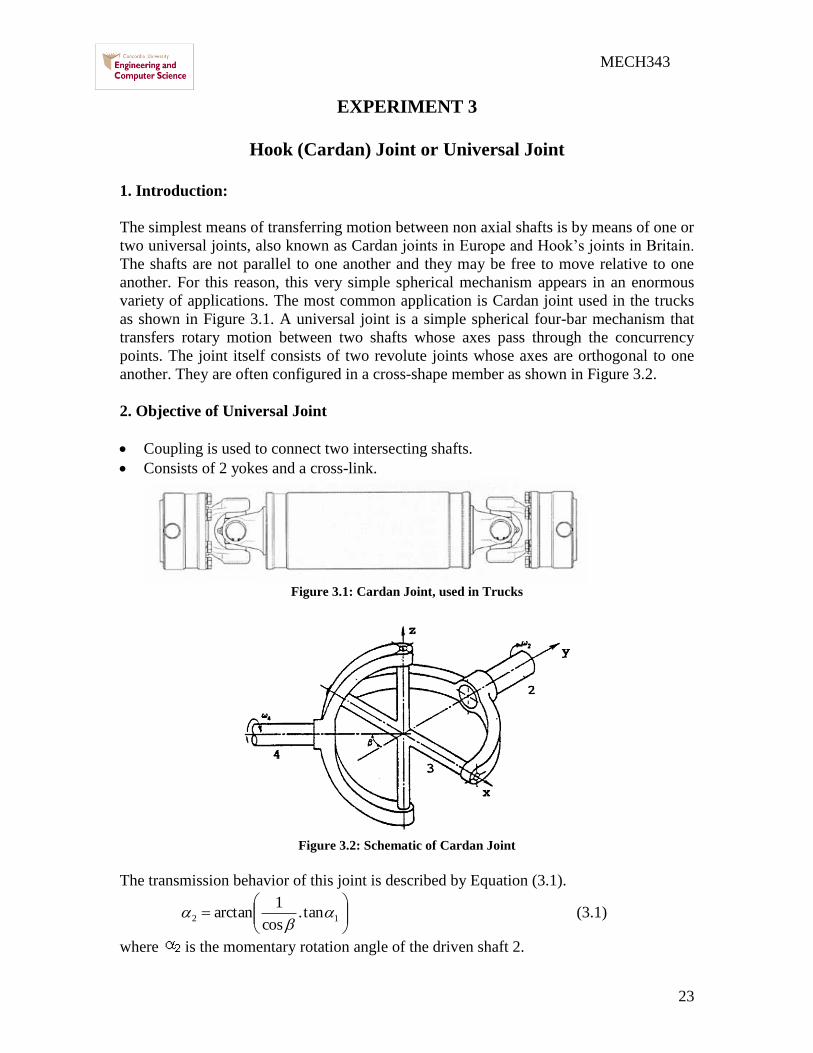
23
MECH343
EXPERIMENT 3
Hook (Cardan) Joint or Universal Joint
1 Introduction
The simplest means of transferring motion between non axial shafts is by means of one or
two universal joints also known as Cardan joints in Europe and Hookrsquos joints in Britain
The shafts are not parallel to one another and they may be free to move relative to one
another For this reason this very simple spherical mechanism appears in an enormous
variety of applications The most common application is Cardan joint used in the trucks
as shown in Figure 31 A universal joint is a simple spherical four-bar mechanism that
transfers rotary motion between two shafts whose axes pass through the concurrency
points The joint itself consists of two revolute joints whose axes are orthogonal to one
another They are often configured in a cross-shape member as shown in Figure 32
2 Objective of Universal Joint
Coupling is used to connect two intersecting shafts
Consists of 2 yokes and a cross-link
Figure 31 Cardan Joint used in Trucks
Figure 32 Schematic of Cardan Joint
The transmission behavior of this joint is described by Equation (31)
12 tan
cos
1arctan
(31)
where is the momentary rotation angle of the driven shaft 2
24
MECH343
Figure 33 Schematic of Cardan Joint
The angular velocity ratio can be described by
22
2
4
sinsin1
cos
(32)
where β is the angular misalignment of the shafts and Ө is the angle of the driving shaft
It is noted that
max2
4
at oo 27090
min2
4
at ooo 3601800 (33)
if β = 0 2
4
= 1 = constant at any Ө
2
4
will vary between a minimum and a maximum during each revolution
ω2 = ω4 only at 4 instants as shown in Figure 34
This is a very big disadvantage in case of automotive vehicles this means that rear
wheels will rotate at variable speed
Figure 34 Relation between
2
4
and Ө
ω2 is constant (because engine and flywheel) speed of car cannot be variable each
revolution because its inertia and so this means tires will slip and severe wear will
happen
25
MECH343
The effect of the angle β can be shown by plotting 2
4
for different values of β (Figure
35)
Figure 35 Relation between
2
4
and β
The acceleration expression of the follower of universal joint for constant ω2 is given by
222
22
24
sinsin1
2sinsincos
(34)
Recall y = u(x)v(x) therefore yrsquo= [vursquo-uvrsquo]v2
For acceleration or retardation
-acceleration when 2Ө lies between 0 -180o
-deceleration when 2Ө lies between 180 -360o
Maximum acceleration occurs when dα4 dӨ = 0 Thus
42
2
maxsin2
sin22cos
forgives
(35)
It is possible to connect 2 shafts by 2 Hooks couplings and an intermediate shaft that the
uneven velocity ratio of the first coupling will be cancelled out by the second Condition
(Figure 36)
42 (36)
Yoke 32 lies in plane containing shaft 2 3
Yoke 34 lies in plane containing shaft 3 4
Figure 36 Two shafts by two Hooks couplings and an intermediate shaft
26
MECH343
2 Objective
Testing the affect of changing of the angle between the shaft and universal joint on the
input and output shaft speed and calculate the speed ration between output and input shaft
speed
3 Experimental Procedure
1) Fixing the input shaft angle 2 0o
2) Setting the output shaft angle 154
3) Filter setting cutoff freq 4 Scope setting ch1 500mv ch2 500mv M 50ms run
scope turn on motor After stable fluctuate signal appear on screen stop scope then
turn off motor
4) Check the input and output shaft speed by using Cursor paired We assume that at
0 N4 is min setting paired cursor at this point as t=0 ms Moving cursor along
ch2 signal and record t and N4 by ∆ __ms __v Fill table 3-1 N2 is input shaft
speed It is constant
5) Repeat step 2 setting the output shaft angle 304 Fill table 3-2
6) Plot the graph of velocity ratio during one cycle for both cases Compare with
theoretical plot using equation 32
Table 3 1 Test results of Cardan joint
154
Table 3 2 Test results of Cardan joint 304
(o) 0 45 90 135 180 225 270 315 360
t (ms)
N4(v)
N2(v)
N4N2
(o) 0 45 90 135 180 225 270 315 360
t (ms)
N4(v)
N2(v)
N4N2
27
MECH343
EXPERIMENT 4
Mechanical Oscillator for Measurement of Friction Coefficient
1 Introduction
The mechanical oscillator is an apparatus which allows the experimental
determination of friction coefficient by measuring the period of an oscillating table As
shown in Figure 41 the apparatus consists of two counter rotating wheels upon which is
placed a table of uniform weight
Figure 41 The mechanical oscillator
If the center of gravity of the table is not centered when it is placed on the rotating wheels
then more of its weight will rest upon one wheel than upon the other Consequently the
frictional forces will not be equal and the table will move in the direction of the larger of
the two forces But the inertia of the table will carry it too far past the center point and the
other wheel will exert the larger frictional force Thus the table will oscillate back and
forth at a frequency which depends upon the coefficient of friction
The basic step to find the equation of motion of the system is to construct the Free Body
Diagram of the oscillating table Figures 2(a) 2(b) and 2(c) show this procedure
Summing the forces in the horizontal plane we have
0RRXg
W21 (41)
or
0XL
W2X
g
W
(42)
hence
0XL
g2X
(43)
28
MECH343
Figure 42 procedure of finding the equation of motion
Since the differential equation of motion of free vibration for a one degree of freedom
system is of the form
02 XX n (44)
where n is the natural frequency of the system then
L
g22
n
(45)
But L
gfn
24 222 (46)
where
f = the frequency of the oscillating table in cps
L = the distances between wheel centers in ft
g = gravity constant
hence 2
22f
g
L (47)
The solution of the equation of motion can be written in the form
tBtAX nn cossin (48)
With the initial condition
00 XandXXt O (49)
one gets oXBandA 0 (410)
The response of the oscillating table is therefore
tL
gXX o
212
cos
(411)
29
MECH343
tL
g
L
gXX o
21212
sin2
(412)
tL
g
L
gXX o
212
cos2
(413)
Thus it may be concluded that the response of the oscillating table is governed by the
initial displacement X0 the coefficient of friction micro and the difference between wheel
centers L
2 Objectives
The experiment is designed to illustrate some of the direct applications of the
theory of vibration to the measurement of physical quantities The experiment also
demonstrates the differences between mathematical models and actual physical systems
Calculate the friction coefficient between the wheels and the bars
3 Description of Experiment
The oscillating table apparatus consists of four grooved wheels mounted on two
axels which are driven by a 120 HP electric motor and a gear reduction unit in opposite
directions The table consists of circular rods connected in a rectangular shape such that
the rods are guided by the grooved wheels
4 Experimental Procedure
1) Measure L the length between the centers of the two wheels
2) Locate one of the bars on the wheels
3) Select two different speeds for the wheels and when it starts rotating and the bar
moving calculate the time for 10 oscillations
4) Calculate the experimental coefficient of friction μ through the following
equation 2
22f
g
L When f is the frequency g gravity acceleration L the
length between the centers of the two wheels Fill table 4-1
5) Find the theoretical coefficient of friction μ for all bars
6) Compare between theoretical and experimental coefficient of frictions μ
Table 4 1 Combinations for measuring the friction coefficient
Case Material of
the bar
Speed
(rpm)
Time taken
for 10
oscillation
Frequency
(f)
Coefficient
of friction
(micro)
Standard
coefficient
of friction
1 Steel
2 Brass
3 Aluminum
30
MECH343
EXPERIMENT 5
5-1 PLANETARY GEAR TRAIN KINEMATICS
1 Introduction
A planetary gear train is one in which the axis of some of the gears may have motion A
planetary gear set always includes a sun gear one or more planet gears and a planet
carrier or arm which sometimes called as sun-and-planet planetary gear train as shown in
Figure1
Figure 51 Planetary gear train
A planetary gear set as shown in Figure 52 is one having two degrees of freedom This
means that the motion of each and every element of the mechanism is not defined unless
the motion of two of its elements is specified To make the planetary set a one degree of
freedom gear train one must fix the motion of one element of the mechanism
Figure 52 Sun-and-planet planetary gear train
2 Solution of Planetary Trains by Formula Methods
Figure 53 shows a planetary gear set which is composed of a sun gear 2 an arm 3 and
planet gears 4 and 5
31
MECH343
Figure 53 Compound Planetary Gear Set
We can express the velocity of gear 2 relative to the arm 3 in the form
3223 nnn (51)
3553 nnn (52)
Dividing Equation (52) by (51) gives
32
35
23
53
nn
nn
n
n
(53)
Since this ratio is the same and is proportional to the tooth numbers it is equivalent
therefore to the train value e
32
35
nn
nne
(54)
Or AF
AL
nn
nne
(55)
where nF = rpm of first gear in train
nL = rpm of last gear in train
nA = rpm of arm
The experiment is designed to demonstrate the fundamentals of planetary gear train and
to show all possible motions that can be obtained with this type of gear trains
3 Objective
Calculate the gear train ratio for the planetary gearbox and the degrees of
freedom that the system has
4 Experimental Procedure
For the planetary gear trains mechanism shown in Figure 51
1) Calculate the degree of freedom to the planetary gear system
2) Calculate the gear train ration through the following equation
21
23
nn
nne
When the outer ring is fixed
When the planet gears are fixed
32
MECH343
5-2 The Borg-Warner Model 35 Automatic Transmission
Simulator
1 Introduction
The Borg-Warner Model 35 Automatic Transmission comprises a three element
torque converter--coupling and a planetary gear set to provide three forward ratios and
reverse
The planetary gear set consists of two sun gears two sets of pinions a pinion
carrier and a ring gear
Power enters the gear set via the sun gears In all forward ratios power enters
through the forward sun gear In reverse it enters through the reverse sun gear Power
leaves the gear set by the ring gear and the pinions are used to transmit power from the
sun gears to the ring gear
In reverse a single set of pinions is used which causes the ring gear to rotate in the
opposite direction from the sun gear In forward ratios a double set of pinions is used to
cause the ring gear to rotate in the same direction as the sun gear
The Carrier locates the pinions relative to the two sun gears and the ring gear also
forming a reaction member for certain conditions The various mechanical ratios of the
gear ser are obtained by the engagement of hydraulically operated multi-disc clutches and
brake bands
Power flow in each ratio is achieved by locking various elements of the planetary gear set
as follows
1st Gear (Lockup selected)
The front clutch is applied connecting the converter turbine to the forward sun
gear The rear band is also applied holding the pinion carrier stationary The gear set
provides the reduction of 239 l The reverse sun gear rotates freely in the opposite
direction to the forward sun gear
33
MECH343
1st Gear (Drive selected)
The front clutch is applied connecting the converter turbine to the forward sun
gear The one-way clutch is in operation preventing the pinion carrier from moving
opposite to the engine rotation The gear set again provides the reduction of 239 1 On
the overrun the one-way clutch unlocks and the gear set freewheels
2nd Gear (Lockup or drive selected)
Again the front clutch is applied connecting the converter turbine to the forward
sun gear The front band is applied holding the reverse sun gear stationary The pinions
now walk around the stationary sun gear and the gear set provides the reduction of 145
l
3rd Gear (Drive selected)
Again the front clutch is applied connecting the converter turbine to the forward
sun gear The rear clutch is applied connecting the turbine also to the reverse sun gear
Thus both sun gears are locked together and the gear set rotates as a unit providing a
ratio of 1 1
Neutral and Park
The front and rear clutches are released and no power is transmitted from the
converter to the gear set
Reverse
The rear clutch is applied connecting the converter turbine to the reverse sun gear
The rear band is applied holding the pinion carrier stationary providing a reduction of
209 l
2 Gear Ratios
119866119890119886119903 119877119886119905119894119900 120579119900120579119894
=1
239
The carrier is held stationary to provide the
reaction member and the gears operate as a
Simple gear train
34
MECH343
The reverse sun gear is held to that the gears
now operate as an epicyclic gear train
For an epicyclic gear train shown as following
119866119890119886119903 119877119886119905119894119900 120579119900120579119894
=1
145
119894134 =
1205961 minus 1205964
1205963 minus 1205964= minus
11988521198851
11988531198852prime
119900119903 120596119871
32
67= 120596119869 minus 120596119871 120596119869 =
99
67120596119871
For our transmission show as above
119894119865119869119871 =
120596119865minus120596119871
120596119869minus120596119871= minus
119885119866
119885119865
119885119867
119885119866
119885119869
119885119867=
67
28 (1)
119894119865119870119871 =
120596119865minus120596119871
120596119870minus120596119871= minus
119885119866
119885119865
119885119867
119885119866
119885119870
119885119867= minus
32
28 (2)
Hence minus120596119871
120596119869minus120596119871= minus
67
68
28
32
From (2) 120596119865 minus 120596119871 =32
28 120596119871 120596119865 =
60
28120596119871
Therefore 119894119865119869 =120596119865
120596119869=
60
28
67
99= 145021645
So 120579119900
120579119894=
1
145
35
MECH343
119866119890119886119903 119877119886119905119894119900 120579119900120579119894
=1
1
Both sun gears are locked together and the
gears set rotates as a unit
119866119890119886119903 119877119886119905119894119900 120579119900120579119894
=1
209
With the reverse gear engaged power is
applied to the reverse sun gear The planet
carrier is held stationary so that the planet
gears rotate the ring gear in the opposite
direction to the reverse sun gear
36
MECH343
3 Experimental Procedure
Pins and slotted plates represent the multi-disc clutches and brake bands The various
gear ratios of the gear set may be obtained by inserting the appropriate pins as indicated
below
A B C D E F
Lockup 1Drive 1
Lockup 2Drive 2
Drive 3
Reverse
Neutral
Park Note
1 Lose all pin and turn input shaft and output shaft make sure input shaft disk and
output shaft disk indicate to 0 then lock pins for each case
2 Turn input shaft one turn (360 ) read output disk (degree)
3 Fill out following table
Input (degree) Output (degree)
Lockup 1Drive 1 360
Lockup 2Drive 2 360
Drive 3 360
Reverse 360
4 Results
According to power flow and gear ratio figures for each case referring to 2nd gear
ratio calculation derive and calculate gear ratios for 1st 3
rd and reverse shift Compare
them with your experimental results
37
MECH343
EXPERIMENT 6
Static and Dynamic Balancing
1 Objective
The objectives of this experiment are
Understanding the concept of static and dynamic balancing
Understanding unbalance torque
Justifying theoretical calculation for balancing with experiment
Balancing the shaft by the four given masses
2 Introduction
Unbalanced dynamic forces effects have profound influence on the working and
of rotating machinery like turbines compressors pumps motors etc These forces act
directly on the bearings supporting the rotor and thus increase the loads and accelerate the
fatigue failure These unbalanced forces induce further mechanical vibrations in the
machinery and connected parts thereby creating environmental noise problem through
radiation of sound Hence it is desirable to balance all such uncompensated masses and
thus reduce the effect of unbalance forces in a dynamics balancing machine
Balancing is the technique of correcting or eliminating unwanted inertia forces which
cause vibrations which at high speeds may reach a dangerous level An important
requirement of all rotating machinery parts is that the rotation axis coincides with one of
the principal axis of inertia of the body After a roll is manufactured it must be balanced
to satisfy this requirement especially for high speed machines The condition of
unbalance of a rotating body may be classified as static or dynamic unbalance
2 1 Static Unbalance
An idler roll is statically balanced if the roll doesnt rotate to a heavy side when free to
turn on its bearings Thus the rolls center of gravity is on the axis of rotation Static
unbalance (Figure 61) creates a centrifugal force when rotating which causes deflection
of the roll Idler rolls are sometimes static
balanced only when the roll operates at slow
speeds
The static unbalance usually happens because
of errors in the manufacturing tolerances of
the rotating parts Therefore static imbalance
is essentially a weighing process in which the
part is acted upon by either gravitational or
centrifugal force This type of unbalance
could be easily reduced or removed by static
balancing
Figure 61 Static (or force) Unbalance
38
MECH343
2 2 Dynamic Unbalance
An idler roll may be in perfect static balance and not be in a balanced state when rotating
at high speeds A dynamic unbalance is a ldquocouplerdquo or twisting force in two separate
planes 180 degrees opposite each other (Figure 62) Because these forces are in
separate planes they cause a rocking motion from end to end A roll that is unbalanced
will cause 1) machinery vibrations 2) web
flutter and 3) a decrease in bearing life due to
unnecessary forces
To dynamically balance a roll it must first be
statically balanced Then the roll must be
rotated to its operating speed and have the
dynamic unbalance eliminated by adding or
subtracting weight The determination of the
magnitude and angular position of the
unbalance is the task of the balancing
machine and its operator Balancing
machines are provided with elastically
supported bearings in which the idler roll may
spin Because of the unbalance the bearings
will oscillate laterally and the amplitude and
phase of the roll are indicated by electrical
pickups and a strobe light
Figure 63 shows a long rotor which is to be mounted in bearing A and B We might
suppose that two equal masses m1 and m2 are placed at opposite ends of the rotor and at
equal distances r1 and r2 from the axis of rotation Since masses are equal on opposite
sides of the rotational axis the rotor is statically balanced in all angular positions But if
the rotor is caused to rotate at an angular velocity ω radsec the centrifugal forces m1r1ω2
and m2r2ω2 act respectively at m1 and m2 on the rotor ends These centrifugal forces
produce the equal but opposite bearing reactions FA and FB and the entire system of
forces rotate with the rotor at the angular velocity ω Thus the rotor is to be statically
balanced and at the same time dynamically unbalanced
Figure 63 Dynamically Unbalanced Rotor
Figure 62 Dynamic (or couple) Unbalance
39
MECH343
3 Principle and Theory of Operation
Consider a body of mass M rotating with a uniform angular velocity about O with
eccentricity e as shown in Figure 64 The centrifugal force Fc acting on the axis of
rotation is Me2 This force is therefore very sensitive to speed and hence there is a need
to reduce this force either by operating at lower speeds or by decreasing the eccentricity
as shown in Figure 65
O
e
M
M e
2
Figure 64 Unbalanced Disc
Center of rotation
( new center of
gravity )
Rotating Disc Added mass m
Center of gravityOriginal center
of gravity
(a) (b)
Figure 65 Illustration of The Simplest Method of Static Balancing
In general it is desirable to make e as low as possible If the rotor thickness to diameter
ratio is less than 05 and speed are below 1000 rpm the rotor can be single plane
balanced - otherwise two-plane balancing is necessary In the single plane balancing
technique with a rotor of mass mi and radius ri from the axis of rotation and lying in the
same plane the condition for static balance is used
0~iirm (61)
where i = 1 2 which denotes the total number of masses and m denotes the mass The
vector ir~ represents the eccentricity e of the mass mi from the axis of rotation
When the bodies are rotating in several planes the condition for dynamic balance has to
be satisfied in addition to that for static balance This is given by
0~~ iii rzm (62)
where iz~ is the axial coordinate vector of the mass mi measured for a chosen datum In
the two-plane balancing technique instead of satisfying Equations (61) and (62)
40
MECH343
explicitly Equation (62) is used with two different datum planes for iz~ Mathematically
if the distance between these two plane is oz~ then
0~)~~( ioii rzzm (63)
It is therefore clear that Equations (62) and (63) imply the satisfaction of Equation
(61) Conceptually it means that if a system of bodies rotating in several planes is in
dynamic balance with respect to two different datum planes then the system is also in
static balance This is the principle of the two-plane balancing technique
4 Description of Experimental Apparatus
Figure 66 shows the Static and Dynamic Balancing Apparatus It consists of a perfectly
balanced shaft with four rectangular blocks clamped to it The shaft is mounted in ball
bearings and it is driven by a 12 volt electric motor through a belt and pulley drive The
shaft assembly is mounted on a metal plate resting on four resilient rubber supports
which allow the mount to vibrate when the shaft is not balanced
The rectangular blocks can be clamped to the shaft at desired out-of-balance moments by
means of discs having eccentric holes of various diameters The discs are fixed to the
blocks by hexagon socket set screws Any longitudinal and angular position of a block
relative to the shaft can be set by linear and protractor scales provided Adjacent to the
linear scale is a slider which can be pushed against the block to read its longitudinal
position The slider also serves as a datum stop against which the blocks can be held
when reading their angular position on the shaft
The out-of-balance moments are measured by fitting the extension shaft and pulley to the
main shaft Each rectangular block is then clamped to the shaft in succession A cord with
a weight bucket at each end is hung on the pulley and bearing balls are placed in the
bucket until the block has turned through 90deg The out-of-balance moment is proportional
to the number of balls required
to turn the block
A Perspex dome serves as the
safety cover The shaft cannot
be driven unless the dome is in
position which is achieved by
micro switches actuated by the
dome The motor switch on the
front panel is spring loaded so
that the motor cannot be left
running The motor requires a
power supply of 12 volts at 2
amperes which is provided by
E66E90 speed controller
Figure 66 Static and Dynamic Balancing Apparatus
41
MECH343
5 Experimental Procedure
5 1 TEST 1 Static Balancing
1 Looking at the shaft from the side the masses will be as shown in figure 6-7
each mass has an angle θ with horizontal
Figure 6-7 Shaft view from the side
2 The masses forces are given by the following table 6-1
The masses values Table 6-1
3 In order to balance the shaft statically the sum of the forces will be equal zero
as the following equations
sum F=0
F1cos θ1+ F2cos θ2+ F3cos θ3+ F4cos θ4=0 (1)
F1sin θ1+ F2 sin θ2+ F3 sin θ3+ F4 sin θ4=0 (2)
4 Since we have just two equations with four unknown angles we assume
θ1=0ordm θ2=90ordm
5 Solving the two equations or using force polygon by AutoCAD to find the θ3
θ4
5 2 TEST 2 Dynamic balancing
1 Looking for the shaft from in front the masses create the forces as shown in
figure 6-8 each mass has an arm X create a momentum
F1
F2
F3
F4
42
MECH343
2 In order to balance the shaft dynamically the sum of the momentum will be
equal zero as the following equations
sum M=0
F1cos θ1X1+ F2cos θ2X2+ F3cos θ3X3+ F4cos θ4X4=0 (1)
F1sin θ1X1+ F2 sin θ2X2+ F3 sin θ3X3+ F4 sin θ4X4=0 (2)
3 Since we have just two equations with four unknown arms we assume
X1=50 mm X2=100 mm
4 Solving the two equations or using momentum polygon by AutoCAD to find
the X3 X 4
TABLE 6 2
Block 1 2 3 4
Mass 88 82 74 64
Angle θ(ordm) 0 90
Arm X (mm) 50 100
6 Typical Calculations
The basic equations that are used for balancing purposes are
0rW ii (63)
0rWa iii (64)
Suppose that block (1) is placed 17 mm from the left end of the shaft at zero angular displacement and that
block (2) is placed 100 mm from it at 120deg The measured out-of-balance moments are as follows
Figure 68 In front shaft view
43
MECH343
TABLE 6 3 OUT-OF-BALANCE MOMENTS
It is first necessary to draw the moment polygon of Wr values as shown in Figure 68 to determine the
angular positions of blocks (3) and (4) W1r1 and W2r2 are known in both magnitude and direction The
vector W1r1 has been drawn at positive X-direction (θ = 0) The lengths of vectors W3r3 and W4r4 are known
and arcs can be drawn from the ends of W1r1 and W2r2 to get the directions of the unknown vectors
Figure 69 shows the diagram of the angular positions and the corresponding longitudinal locations of the
blocks on the shaft are 17 mm for the first 117 mm for the second block
To find the longitudinal positions of the other two blocks we designate distance of block (3) by a3 and
distance of block (4) by a4 measured from block (1) so block (1) is the reference and will not appear in
calculations
Draw a vector a2W2r2 = 100 (82) units long parallel to r2 and vectors a3W3r3 and a4W4r4 parallel to r3 and r4
respectively so that the moment polygon is closed The lengths of vectors a3W3r3 and a4W4r4 can be
measured and the magnitudes found by using the scale factor From these a3 and a4 can be calculated
Notice that the sense of vector a3W3r3 is reverse In order to maintain vector a3W3r3 the only possible
solution is to reverse a3 So from the vector polygon (triangle) it follows
a3 = -12 mm
a4 = 124 mm
This means that block (3) should be located 5 mm from the left end of the shaft The blocks should be
positioned as follows
Block Angular Position (Deg) Longitudinal Position (mm)
(1) 0 17
(2) 120 117
(3) 190 5
(4) 294 141
The values of a3 and a4 can be found analytically using complex vector approach
Real and imaginary components yield
100(82) cos 120deg + (74) a3 cos 190deg + (64) a4 cos 294deg = 0
100(82) sin 120deg + (74) a3 sin 190deg + (64) a4 sin 294 deg = 0
which reduce to
4100- 7288 a3 -2603 a4 = 0
71014- 1285a3 -5847 a4 = 0
44
MECH343
Solving the two equations gives a3 = -1194mm a4 = 12396mm
The values compare very well with those obtained graphically
In order to obtain independent results it is suggested that Wr values of the blocks are varied by using
different positions of the discs with eccentric holes The angular displacements between blocks (1) and (2)
may also be varied
Figure 69 Moment Polygon of Wr
45
MECH343
EXPERIMENT 7
Machine Fault Simulator (MFS)
1 Theory
Refer to experiment number 6
2 Description of Experimental Apparatus
Figure 71 shows the machine fault simulator The rotor is driven by a variable speed
motor via a flat belt and the rotor rotational speed is captured through a digital
tachometer The vibration due to the unbalanced rotor is measured and fed directly into
the on-board processor of the machine
Figure 71 Machine Fault Simulator
3 Objective
In this experiment we will study the reaction of the shaft and the motor when the shaft is
balanced and when it is unbalanced
4 Experimental Procedure
1) Run the Vibro-Quest Software
o Define a ldquoNew Projectrdquo (under root)
o Fill up the window select ldquoProject namerdquo click ldquoNextrdquo
o Select ldquoNonerdquo from the menu on the right side click ldquoNextrdquo
Belt
Motor
Disk A Disk B
Reciprocating
Mechanism
Speed
Control
46
MECH343
o Review the table (do not change the default) click ldquoNextrdquo
o Review the table check the setting data click ldquoNextrdquo
o Click ldquoDonerdquo
o Review the information provided if they are not ok ldquoGo backrdquo to modify
the data then click ldquoFinishrdquo
2 Select ldquoDatardquo from the toll bar on the computer
3 Name the ldquoTest Titlerdquo in the window Insert the parameters used in the test and
click ldquoNextrdquo
4 Review the information provided in the window and click ldquoNextrdquo
5 Chose 2000 as Frequency limit 1600 for Space line Leave the rest information as
defaulted and ldquoGO DAQrdquo
2) Running the Machine Fault Simulator
Select the required speed (rpm) change it to frequency (Hz) using the following
relation 60)rpm(n2)Hz(f
1 Run the machine using speed control system at desired speed
2 Wait about 15 seconds to stable the system
3 Click onrdquo START RECORDINGrdquo
4 When the recording is finished save the file under the root of ldquoDatardquo of base line
at the subdirectory that you want to compare with the other data (for example if
you are running the machine at 20 Hz save the your file under 20 Hz subdirectory)
5 Now select the ldquoProject namerdquo from the left menu all the relevant tests will
appear at the right table under the ldquoTest Explorerrdquo
6 To compare the data from different files Hold down the ldquoShiftrdquo key and select
any two interested files that you are going to compare
7 Click on ldquoComparerdquo to observe the difference between the unbalanced system
with a base system
8 To observe more clearly the difference between the frequency responses of the
different test click on ldquoOverlayrdquo
TEST 1 Imbalance Effects on Vibration response
Install the defined weight in one of the taped hole in rotor disk A and tight it
securely with a nut
Close the cover of MFS
Change the motor speed and record vibration level at each bearing For this
purpose you don not need to define new project for each speed define a new
project( follow steps 1-6 from section 3) then follow steps 1-2 for each speed
from section 4
Measure the average level of amplitude at each speed and Plot it against the speed
Repeat steps 2-5 for 2 different weights at 2 different radius and angles
47
MECH343
TEST 2 Balancing the Imbalance Rotor
Add weight at different radius and angles using the ldquosample calculationrdquo to
balance the rotor
If the rotor is balanced define a ldquoNew projectrdquo and follow steps 3-8 of Section 4
Fill Table 7 1
TABLE 7 1
Unbalance weight on disc A ____________ angular position _______________
Mass Added on disk B gr r (mm)
Amp baseAmp New
48
MECH343
EXPERIMENT 8
DETERMINATION OF SPUR GEAR EFFICIENCY
1 Objective
The main objective of the experiment is to determine the efficiency of the
Spur gear and worm gear unit
2 Introduction and theoretical background
21 Pinion gear
Two intermeshed toothed wheels make up a pinion gear This type of gear
permits a positive transmission of motion and torque Wheel pairs are available in
different shapes and shaft configurations Figure 1 explains the various types of gears and
their arrangements
Fig8 1 Various types of gear arrangements
22 Worm gear
A worm gear is a screw-type transmission unit whose axes generally intersect at
right angles The worm and wheel make contact on a straight line Normally the worm
has a cylindrical core and the wheel globoid toothing Units with a very high performance
49
MECH343
consist of a globoid worm and globoid wheel A worm gear with a cylindrical worm has
the following special features
High load capacity compared with spur gears due to linear contact
Low-noise operation and high absorption of vibrations
Wide transmission range down to low ilt110
High efficiency at high transmission ratios high efficiencies(η le 98 ) can be
achieved with very sophisticated designs under favorable operating conditions a
decrease in pitch angle (high transmission ratio) or speed is accompanied by a
corresponding decrease in efficiency (to η le 50 )
Self-locking operation
Smaller and lighter design compared with spur bevel gear units possessing high
transmission ratios
23 Basic definitions
Drive torque
The drive torque is the product of the force F and the lever arm l on which the
force acts
M = F X l (1)
M is in Nm F is in N and l in m
Drive power
The drive power of a rotating shaft is the product of the torque M and angular
frequency ω P = M X ω (2)
and 60
2 n (3)
P is in W n is in rpm
Efficiency
The efficiency is defined as the ratio between the output and input powers It has a
maximum theoretical value of 1
in
out
P
P (4)
where speed i
nn 1
2
50
MECH343
3 Experimental set-up
Figure 2 shows the complete view of the experimental set up
Fig8 2 Complete view of GUNT AT 200 experimental set up
The modules comprising the drive unit spur gear worm gear and magnetic
powder brake are mounted on a profile frame The DC shunt motor is designed for right-
hand and left-hand rotation The drive unit is electrically powered via control housing
The control unit adjusts the DC machinersquos speed via its armature voltage Its target speed
is set by means of a potentiometer on this housing Its actual speed is measured and
indicated by means of an inductive proximity switch and evaluation unit The speed is
51
MECH343
measured inductively by a contactless sensor disc and indicated by a digital display
element on the control unit Electronic thyristor speed control with I x R compensation
provides a high torsional rigidity The reaction torque exerted on the drive housing is
measured by means of a spring force meter connected to a lever arm
The transmission units consist of a 2-stage spur gear with transmission
ratio i = 135 and a single-stage worm gear with transmission ratio i = 14The
transmission torque can be determined on the drive side as well as the brake side To
facilitate adjustment of the brake torque the brake characteristic (current torque) is
recorded in a preliminary experiment Moments are determined through power
measurements (spring balance) with a known lever arm The moments measured input
speeds and transmission ratios are used to determine power and efficiency
The magnetic powder coupling consists of two independently mounted
rotors ie a primary and a secondary rotor both furnished with ball bearings The
primary rotor also serves as a coil carrier If one of these two rotors is deactivated the
magnetic powder coupling can also be used as a brake The air gap between the two
rotors contains a special magnetic powder If a direct voltage is applied to the excitation
winding the powder aligns itself with the resulting magnetic field lines to form a
compact mass providing a frictional link between the primary and secondary rotors The
value of the torque depends on the adjusted current When the current-proportional
moment is exceeded slippage occurs without any transition
4 Experiments procedure
As shown in Figure 82 the complete view of the experimental set up for this
experiment there is input as the motor speed and the output as excitation current so that
there is two steps for this experiment
After making sure spur gear is connected as shown in Figure 83
1) Fix the output excitation current at I= 50 mA and change the speed of the motor as
shown in the table (1) each time measure the motor force F1 and the brake force F2
52
MECH343
Figure 83 Configuration of spur gear unit experimental set up
Measurement data to determine the efficiency of Spur gear unit Table (1) I = 50mA
SlNo Motor speed
( n1 ) rpm
Motor holding
force ( F1 ) N
Brake holding force
( F2 ) N
Efficiency ( η )
1 500
2 1000
3 1500
4 2000
5 2500
In order to find out the spur gear efficiency we go through the following equations
The general equation for the spur gear efficiency is
in
out
P
P
The drive power of a rotating shaft is the product of the torque M and angular
frequency ω P = M X ω
The drive torque is the product of the force F and the lever arm l on which the
force acts
M = F Arm
When the arm for the motor Arm1=25 mm and for the brake Arm2=50 mm
53
MECH343
And the angular velocity from the following equation
60
2 n
In order to find the speed for the brake we use this ratio assuming i= 135
i
nn 1
2
2) Fixing the input n1= 1500 rpm and changing the output and filling table (2)
Recorded values of the excitation current and the force on the lever arm table (2)
Speed n1= 1500 rpm
Excitation current I (mA) Force F2 on the lever arm (N)
50
70
90
110
130
150
130
110
90
70
50
5 Experiments Results
1) Plot the characteristics curve between the current I and the force on the lever arm
F2
2) Plot the characteristics curve between the current I and the torque M
3) Determine the efficiency of the spur gear unit Comment on the errors on the
efficiency if the calculated efficiency deviates from the realistic values of 80 -
90
54
MECH343
EXPERIMENT 9
ANALYSIS OF LINKAGE MECHANISM
Try to build a linkage mechanism as the figure below
Steps
1 Turn on grid line from View-workspace-grid lines as below
2 Select rectangle tool
55
MECH343
3 Click and drag a small rectangle
4 Click the rectangle copy it (CTRL+C) paste it (CTRL+V) two times
5 Change the length of each rectangle by selecting it and writing down the desired
length in the text box named W
Make the length as (3 ndash 332 - 4)
56
MECH343
6 Use the rotate tool and the select tool to arrange the rectangles
Make sure that the spacing is 4 units as shown below
7 Put a motor at the lower end of the left link
- First select the motor - Then click at the desired point
57
MECH343
8 Put a pin joint at the lower end of the right link
- First select the pin joint - Then click at the desired point
9 Put a point element at the remaining ends
- First double click (this
enable you to assign multiple
points) on the point element
It should look like below
58
MECH343
10 Join the links by selecting two points then selecting Join
Click the arrow select tool
Select first point ndash
press SHIFT and
click the other point
Press
Join
They should look like
below
11 Repeat the same for the remaining two points Your model should look like below
59
MECH343
12 Click RUN ( ) and watch it rotating
13 Now we want to capture the velocity of the joint between the left link and the middle
one
- Select it and click on Define ndash Vectors-
Velocity
Click Run and watch the velocity change
Note that by clicking on the link itself and defining the velocity the program calculates
the velocity of the CG of the link
14 Now you are ready to try different measurements
Acceleration Total Force Gravitational Force
60
MECH343
15 Select a link and use the measure tool
X- Position Graph
Y- Position Graph
61
MECH343
Measuring velocity values
16 Now try to change the length of any of the links and RUN the model and observe
for any change if any and explain
17 Change the mass of any of the links and observe for any change in velocity and
force And Why if there is any
18 Now double click on the motor (resetting the mass for any link that has been
changed) and notice that the value for velocity is 1 radsec Change this to make it the
same value for acceleration and torque Write what you observe and try to explain
19 Now increase the mass for one link (eg left one) gradual and see how this will
affect the motion for a fixed value for torque velocity or acceleration of the motor
20 Now replace the middle link with two links connected with total length as the
middle one run observe and explain
21 Based on (20) search for what is the equation relation or rule that governs the
mechanism motion
62
MECH343
EXPERIMENT 10
NUMERICAL DYNAMIC SIMULATION FLYWHEEL
Problem Definition
In the two cycle piston engine shown explosive gases are
ignited in the combustion chamber above the piston The
explosions apply a force of 150 N for the duration of every
downward stroke The engine is equipped with a speed
limiting device (rev limiter) which prevents the rotational
speed from exceeding a set value (red-line) The masses of
the piston and connecting rod are 075 kg and 15 kg
respectively The mass of the crankshaft-flywheel assembly
is 30 kg Given that the red-line of the engine is 35 radsec
(340 rpm) Assume the crankshaft-flywheel assembly can
be modeled as a circular disk
Objective
Determine the forces at the crankshaft bearing (point A) and connection rod (point B)
bearing
Solution
1 INTRODUCTION
Engines that exceed the manufacturers maximum speed (over-revving) may be subject to
excessive wear and possible failure To prevent over revving internal combustion
engines are often fitted with a device known as a rev-limiter When an engine exceeds its
red-line rev-limiters interrupt the ignition system slowing the engine down Once the
speed drops below the maximum the ignition system is switched back on In this exercise
you will model an internal combustion engine equipped with a rev-limiter The engine
has three bodies the piston the connecting rod and the crankshaft The piston will be
modeled by a square body The connecting rod will be modeled by a rectangular body
The crankshaft will be modeled as a circular body The bodies will be drawn sized and
joined to each other and the background The pistons cylinder walls will be modeled with
a keyed slot joint The force of combustion will be modeled by a force attached to the top
of the piston The resulting forces at the bearings will be measured
2 SETTING UP THE WORKSPACE
For this exercise three changes in the workspace will be made First for clarity the x-y
axes will be displayed The unit of distance will also be changed from meters (default) to
millimeters
63
MECH343
If the x-y axes are not currently displayed choose Workspace from the
View menu and choose XY Axes from the Workspace submenu The x-y
axes provide a reference frame for building a simulation
Choose Numbers and Unitshellip from the View menu The Numbers and
Units dialog appears
Click the More Choices button The dialog box expands
Click and hold in the Distance field (Figure 1) The pop-up menu appears
Choose millimeters from the Distance pop-up menu
Click in the Rotation field and choose Radians from the pop-up menu
Click OK
3 CREATING THE COMPONENTS
This exercise has three objects a 15 kg connecting rod a 075 kg piston and a 30 kg
crankshaft (see Figure 2 below) The connecting rod will be modeled by a thin rectangle
400 mm in length Its width will be thin 150 mm so it closely resembles the actual
connecting rod The crankshaft as stated in the exercise is modeled as a circular disk
with a 200 mm radius and a mass of 30 kg A 200 mm square object will represent the
piston The objects will be created sized and initialized in the following steps
Creating the Crankshaft
The crankshaft is represented by a circle with a radius of 200 mm and mass of 30 kg
These parameters will be set using the Geometry and Properties utility windows
I To draw the crankshaft
64
MECH343
bull Click the Circle tool in the Toolbar
bull Click once on the background Move the mouse to expand the circle and click
again to complete sketching
II To set the mass of the crankshaft
Choose Properties from the Window menu
Click the mass field and enter the value 30
III To set the size of the crankshaft
Select the crankshaft if it not already selected
Click the Radius field (labeled ldquorrdquo) of the Coordinates bar and enter the value 200
(Figure 3)
IV Zooming In
The circle will appear small after sizing To make the rectangle easier to manipulate and
appear larger the workspace will be magnified using the Zoom tool To zoom in
Click the Zoom In tool in the Toolbar
Click near the circle The objects in the window are magnified by a factor of two with
each click of the mouse To zoom out while the Zoom In tool is selected hold down
65
MECH343
the Shift key (the magnifying glass pointer changes to ldquo-rdquo) and click Your screen
should be similar to Figure 4 below
Figure 4 The workspace after zooming in
Click the Arrow tool in the Toolbar or press the spacebar to deselect the Zoom In
tool
Creating the Piston
For this exercise the piston will be modeled as a 200 mm square with the mass of 75 kg
The Square tool will be used to draw the piston and the Properties window will be used
to set its mass
I To draw the piston
Choose the Square tool in the Toolbar On systems the Square tool is ldquohiddenrdquo in the
RectangleSquare pop-up palette by default Click and hold on the Rectangle tool to
bring the pop-up palette in view (Figure 5 below)
Click once on the background drag to the right and click again to complete
sketching A square appears on the screen To set the size of the piston
Click in the Height or Width field of the Coordinates bar and enter 200 Either field
changes both the height and the width of the object so that it remains square
Figure 5 RectangleSquare pop-up palette
II To set the pistonrsquos mass
bull Select the piston if it not already selected
bull Choose Properties from the Window menu
66
MECH343
bull Click in the mass field and enter the value 075
Creating the Connecting Rod
In this exercise the connecting rod is represented by a rectangle drawn with the
Rectangle tool and sized using the Geometry window To approximate an actual
connecting rod the rectangle will be given a mass of 2 kg a height of 500 mm and a
width of 100 mm
To draw the connecting rod
I Choose the Rectangle tool in the Toolbar (On systems the Square tool used above
may have replaced the Rectangle tool in the Toolbar If so the Rectangle tool may be
selected from the hidden pop-up palette by clicking and holding on the Square tool in
the Toolbar)
II Click once on the background drag to the right and click again to complete
sketching A rectangle appears on the screen To set the mass of the connecting rod
bull Select the new rectangle if it not already selected
bull Choose Properties from the Window menu
bull Click in the Mass field and enter the value 2
To set the size of the rod
1 Click the Height field of the Coordinates bar and enter the value 500
2 Click the Width field of the Coordinates bar and enter the value 100 Your screen
should resemble Figure 6
Figure 6 The piston crankshaft and connecting rod
Creating the Points for Joining
The objects in this exercise are connected to each other and to the background (see Figure
7 below) The connections will be modeled by creating points and joining them These
points will be created with the Point tool and accurately positioned using the Properties
window
67
MECH343
Figure 7 The points which will be created and their coordinates
Creating Points on the Connecting Rod
Double-click the Point tool in the Toolbar Double-clicking selects a tool for
successive operations On systems the difference between single and double-clicking
is indicated in the Toolbar by shading a doubleclicked item is dark grey while a
single-clicked item is light grey
Place the mouse pointer over the connecting rod rectangle Find the snap point at the
top end of the connecting rod An X symbol appears at snap points Find the snap
point located at the midpoint of the top side of the connecting rod
To attach a point element click when the snap point located at the top end is visible
Observe that the point element is attached to the top end of the rod
In the same fashion attach another point element to the bottom end of the connecting
rod Your screen should resemble Figure 8
Figure 8 Connecting rod points in position
68
MECH343
Attaching Points to the Crankshaft
The crankshaft needs two points a center point representing the main bearing and an
outer point representing the connecting rod bearing These points will be accurately
positioned at the center and at 200 mm from the center of the circle To create and
position the crankshaft points
Make sure the Point tool is still selected Place the mouse pointer over the
crankshaft Find the snap point at the center of the circle
Click when the snap point at the center is visible A point element is attached to
the center of the circle
Place the mouse pointer near the left quadrant of the circle Find the snap point at
the left quadrant (Figure 9) As the mouse pointer nears the left quadrant of the
circle the snap point appears
Click when the snap point at the left quadrant is visible Another point element is
attached to the left quadrant of the circle
Figure 9 Snap point at the left quadrant of the circle
Attaching Points to the Piston
Two points need to be attached to the piston a square point and a point The square point
will be joined to the slot on the background to create a keyed slot joint The point will be
joined to another point on the connecting rod to form a pin joint The square point will be
positioned on the piston at the coordinates of (0 -50) The square point will be rotated 90deg
so that when joined to the slot the piston will not rotate This is because vertical slots are
defined as being rotated 90deg horizontal slots are defined as having 0deg rotation When a
square point is joined to a slot the rotations of the two objects are aligned
I The point will be positioned at (0 0) To create the points
Click the Square Point tool The cursor turns into a square point
Click anywhere on the piston Since the square point will be precisely position
using the Coordinates bar below it is not necessary to find a snap point
Click in the X field of the Coordinates bar and enter 0 If you attached the square
point on a snap point the x-field of the Coordinates bar may contain a formula
expression (such as body[3] width or (00)) Simply overwrite the entire
expression and enter 0
Press the tab key to move to the Y field of the Coordinates bar and enter -50
Again simply overwrite the y-field with the value -50
Choose the Properties in the Window menu The Properties window appears
In the angle field of the Properties window (marked by oslash) enter the value 1571
The value of 1571 radians is equivalent to 90deg The value will be displayed in a
69
MECH343
rounded form but internally the correct value will be used The pointrsquos y-position
is set to -50 so it will not interfere with the connecting rod joint
II To create the point
Click the Point tool
Place the pointer near the center of the square and find the snap point
Click when the snap point at the center is visible The point is created at the center
of the piston
Attaching a Point to the Background
A point representing the main bearing of the crankshaft must be placed on the
background The point can be placed anywhere on the background for clarity it will be
placed at the origin (0 0) To create and position the point
Click the Point tool
Place the mouse pointer near the origin Find the snap point that appears at the
origin Make sure that nobody is obstructing the origin The snap point does not
appear if the origin is covered by a body
Click when the snap point at the origin is visible Verify the position of the point
by noting the (x y) position in the Coordinates bar it should be (0 0) We now
name this point element so that it becomes easier to select later
Choose Appearance from the Window menu The Appearance window appears
In the name field (where it says Point) type Base Pin Since we will not be
needing the Appearance window for the rest of the exercise close the window by
(Windows) clicking the box marked ldquoXrdquo at the top-right corner of the window or
() clicking the box at the top-left corner of the window
Attaching a Slot to the Background
The cylinder walls of the engine will be modeled with a keyed slot joint The joint will be
made by joining the square point on the piston to a slot attached to the background The
slot can be located anywhere on the background as long as it is located on the
crankshaftrsquos centerline (the yaxis for this model)
To create and position the slot on the background
Choose the Vertical Slot tool in the Toolbar On systems the Vertical Slot tool
may be ldquohiddenrdquo in the Slot pop-up palette Click and hold on the Slot tool in the
Toolbar to bring the pop-up palette in view
Place the pointer near the point element attached to the origin Find the snap
point
Click when the snap point is visible A vertical slot appears
Creating Joints
In this exercise there are four joints (see Figure 10) The joints will connect the piston to
the slot the piston to the connecting rod the connecting rod to the crankshaft and the
crankshaft to the main bearing
70
MECH343
Figure 10 The points which will be joined
The following steps will demonstrate how to make these joints
I Joining the Piston to the Slot
In this example the piston slides in a cylinder The
cylinder will be modeled as a keyed slot joint The joint
is created by joining the square point on the piston to the
slot To create the keyed slot joint
Select the square point on the piston and while
holding down the Shift key select the slot The word
ldquoJoinrdquo of the Join button in the Toolbar changes
from gray to black indicating the two points can be
joined
Click the Join button in the Toolbar The piston
moves to the slot (see Figure 11) Joining the
Crankshaft to the Point on the Background The
crankshaft main bearing is modeled as a pin joint
The pin joint will be created by joining the point at
the center of the circle to the point at the origin
II To join the crankshaft to the origin
Choose Properties in the Window menu
From the selection pop-up menu located at the top of the
Properties window choose Base Pin (Figure 12) The
Base Pin is now selected
Hold the Shift key down and select the center point on
the crankshaft circle
Click the Join button The crankshaft circle moves to the
origin
To see how the circle representing the crankshaft is
constrained bring the mouse pointer over the circle hold
down the mouse button and drag the circle The circle
can rotate but is fixed to the Base Pin
Figure 11 Piston joined to the slot
Figure 12 Selecting an object in
the Properties window
71
MECH343
III Joining the Components
The piston connecting rod and crankshaft will now be joined together (see Figure
13) The following steps describe how to join them
Figure 13 Joining the components
IV To join the piston to the connecting rod
Select the (round) point on the piston and while holding
the Shift key down select the top point on the
connecting rod
Click the Join button The two objects will come
together
V To join the connecting rod to the crankshaft
Select the bottom point on the connecting rod and while
holding the Shift key down select the remaining (left)
point on the crankshaft
Click the Join button Your screen should resemble
Figure 14
Editing the collision property of a pair of bodies
The Smart Editor keeps joints together during editing To see this try dragging the
connecting rod The connecting rod will stay joined while it is dragged and the crankshaft
and piston will move accordingly When you are done dragging the rod move it back to
the approximate position shown in the problem description on the first page of this
exercise
Preventing a Collision
In Working Model objects which are directly connected to each other never collide
Notice that the piston and crankshaft may overlap when they are dragged during editing
Since the two objects are not directly connected they will collide when you run the
simulation To prevent the collision the Do Not Collide command will be used
To prevent a collision
Select the piston and while holding the Shift key down select the crankshaft
Figure 14 the completed engine
72
MECH343
Click and hold on the Object menu title in the menu bar (Figure 15) Notice that
there is a checkmark beside ldquoColliderdquo indicating that the pair of selected objects
will collide when you run the simulation
Choose Do Not Collide in the Object menu
Figure 15 Editing the collision property of a pair of bodies
Creating the Force
A 100 N force is applied at the top of the piston in the negative y-direction (down) The
force is only active while the piston is traveling with a negative y velocity The force will
be drawn using the Force tool and its magnitude and location will be set using the
Properties window
Drawing the Force
The force will be drawn in the downward direction using the
Force tool
To draw the force
Click the Force tool in the Toolbar
Place the pointer near the midpoint of the top end of
the piston Find the snap point
Click when the snap point is visible drag the mouse
upward and click again to create the force A force
attached to the piston appears (Figure 16) Do not be
concerned with the exact direction or magnitude of the
force for now
Sizing the Force
The forcersquos magnitude and direction will be set using the Coordinates bar To size the
force
bull Click the force vector to select the force
bull Click the Fy field of the Coordinates bar and type -100
bull Click the Fx field of the Coordinates bar and type 0 The force vector changes in
length to reflect its new magnitude
Figure 16 Creating a Force
73
MECH343
Timing the Force
The ignition timing of the engine must be simulated The problem states that the force is
active only on the downward stroke (ie when the piston has a negative velocity) The
rev-limiter cuts off combustion when the rotational velocity is greater than 35
radianssecond To simulate these conditions the ldquoand (ab)rdquo function will be
incorporated with the following formulas
To determine when the piston has a negative velocity use the following formula
body[c]vy lt 0
where c is the pistons object id number To determine the pistonrsquos id number place the
cursor over the piston and read the Status bar
To determine when the enginersquos speed is greater than 35 rads use the following
formula
body[d]vr lt 35
where d is the crankshafts object id number Use the Status bar as above to determine the
crankshaftrsquos id number
The complete equation is
and (body[c]vy lt 0 body[d]vr lt 35)
The complete equation will be placed in the Active When field in the forcersquos Properties
window Gravity will provide the initial downward velocity to start the engine
To set the timing of the force
Select the force
Choose Properties from the Window menu
Click in the Active When field at the bottom of the Properties window On
Windows systems you must first un-check the Always button before clicking in
the Active When field
Type the following formula (see Figure 17)and(body [c]vy lt0body[d]vrlt 35)
where c and d are the object id numbers of the piston and crankshaft respectively
The forcersquos rev-limiter equation is designed for counter-clockwise (positive)
engine rotation It is important that the
engine be ldquostartedrdquo in a position similar to
the figure on the first page of this section
If you want a rev-limiter which works in
both directions try incorporating the abs()
function into the formula
You can increase the width of the ldquoActive
whenrdquo field to view the entire equation by
resizing the Properties window
The simulation is ready to run
Click the Run button in the Toolbar The engine runs A warning may appear if
you run the engine long enough you can ignore the warning for now
When you are ready to continue click the Reset button in the Toolbar
Figure 17 Active When field is in
the property window for a Force
74
MECH343
Measuring Properties from the Simulation
A graph in conjunction with a digital meter is a nice way to illustrate the rotational speed
of the enginersquos crankshaft Two digital meters will be used to display the forces on the
bearings Follow the steps below to create these output devices
Displaying a Graph
The angular velocity of the crankshaft will be
displayed by a graph To create the graph
Select the crankshaft circle Four squares
ldquohandlesrdquo will appear around the circle
indicating that the circle is selected
Choose Velocity from the Measure menu
and Rotation Graph from the Velocity
submenu A meter resembling Figure 18
appears
Displaying Digital Force Meters
To display the digital force meters
bull Select the crankshaft-main bearing joint (see Figure 19)
bull Choose Force from the Measure menu A digital meter appears
bull Repeat for the connecting rod-crankshaft joint (see Figure 19)
A second digital meter appears You may need to move the meters
To move the meters
bull Select a meter
bull Drag it to any position you wish
Your window should resemble Figure 20
Running the Simulation
Run the simulation Notice that the angular velocity increases until it reaches 30 rads
This is so because we have turned off the force above 30 rads just as a rev limiter t urns
off the ignition of an engine above a certain speed
Figure 18 A Velocity Graph
Figure 19 The Force to be measured Figure 20 The completed workspace
75
MECH343
Modifying the Graph Display
You may notice that the axis labels occlude the numeric labels along the tick marks of the
plot You can modify the display options using the Appearance window For example to
turn off axis labels so that the numeric labels clearly appear
Select the velocity meter on the screen
Choose Appearance in the Window menuAlternatively you could press
Control+J (on Windows systems) or Command+J (on MacOS systems) to open
the window
Turn off the options titled ldquoLabelsrdquo and ldquoUnitsrdquo (Figure 21) You may wish to try
modifying other options and observe the effects on the graph meter
If you wish to show the meter coordinate axes click the check box labeled Axes
MODIFYING THE SIMULATION
Try modifying the masses of the crankshaft and connecting rod and notice how quickly
red-line is reached Also try changing the length of the connecting rod by repositioning
one of the joints
Figure 21 Appearance window for a meter
76
MECH343
Appendix
A Running the VibroQuest Software
1 Run the VibroQuest 2 New Project (under root)
3 Fill up the window click ldquoNextrdquo 4 Select ldquoNonerdquo click ldquoNextrdquo
1 2
3
4
5
6
77
MECH343
5 Review the table (do not change the default) click ldquoNextrdquo
6 Click ldquoNextrdquo
7 Click ldquoDonerdquo
8 Click (review the information provided if they are not ok go back to modify them)
ldquoFinishrdquo
B Run the machine according to the procedure
9 Select ldquoDatardquo from the toll bar on the computer
10 Name the ldquoTest Titlerdquo in the window Insert the parameters used in the test and click
ldquoNextrdquo
7
8
9
1
0
78
MECH343
11 Review the information provided in the window and click ldquoNextrdquo
12 Chose 2000 for Frequency limit 1600 for Space line Leave the rest information as
defaulted and ldquoGO DAQrdquo
13 ldquoSTART RECORDINGrdquo
14 When the recording is finished save the file under the root of Data of the file which
you are to compare with
15 Now select the project name from the left window all the relevant tests will appear at
the right window
16 Hold down the shift key and select two tests that you are going to compare
17 Click on Compare to observe the difference between the unbalanced systems with
base system
1
1 1
2
1
3
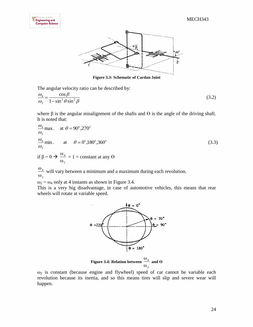
24
MECH343
Figure 33 Schematic of Cardan Joint
The angular velocity ratio can be described by
22
2
4
sinsin1
cos
(32)
where β is the angular misalignment of the shafts and Ө is the angle of the driving shaft
It is noted that
max2
4
at oo 27090
min2
4
at ooo 3601800 (33)
if β = 0 2
4
= 1 = constant at any Ө
2
4
will vary between a minimum and a maximum during each revolution
ω2 = ω4 only at 4 instants as shown in Figure 34
This is a very big disadvantage in case of automotive vehicles this means that rear
wheels will rotate at variable speed
Figure 34 Relation between
2
4
and Ө
ω2 is constant (because engine and flywheel) speed of car cannot be variable each
revolution because its inertia and so this means tires will slip and severe wear will
happen
25
MECH343
The effect of the angle β can be shown by plotting 2
4
for different values of β (Figure
35)
Figure 35 Relation between
2
4
and β
The acceleration expression of the follower of universal joint for constant ω2 is given by
222
22
24
sinsin1
2sinsincos
(34)
Recall y = u(x)v(x) therefore yrsquo= [vursquo-uvrsquo]v2
For acceleration or retardation
-acceleration when 2Ө lies between 0 -180o
-deceleration when 2Ө lies between 180 -360o
Maximum acceleration occurs when dα4 dӨ = 0 Thus
42
2
maxsin2
sin22cos
forgives
(35)
It is possible to connect 2 shafts by 2 Hooks couplings and an intermediate shaft that the
uneven velocity ratio of the first coupling will be cancelled out by the second Condition
(Figure 36)
42 (36)
Yoke 32 lies in plane containing shaft 2 3
Yoke 34 lies in plane containing shaft 3 4
Figure 36 Two shafts by two Hooks couplings and an intermediate shaft
26
MECH343
2 Objective
Testing the affect of changing of the angle between the shaft and universal joint on the
input and output shaft speed and calculate the speed ration between output and input shaft
speed
3 Experimental Procedure
1) Fixing the input shaft angle 2 0o
2) Setting the output shaft angle 154
3) Filter setting cutoff freq 4 Scope setting ch1 500mv ch2 500mv M 50ms run
scope turn on motor After stable fluctuate signal appear on screen stop scope then
turn off motor
4) Check the input and output shaft speed by using Cursor paired We assume that at
0 N4 is min setting paired cursor at this point as t=0 ms Moving cursor along
ch2 signal and record t and N4 by ∆ __ms __v Fill table 3-1 N2 is input shaft
speed It is constant
5) Repeat step 2 setting the output shaft angle 304 Fill table 3-2
6) Plot the graph of velocity ratio during one cycle for both cases Compare with
theoretical plot using equation 32
Table 3 1 Test results of Cardan joint
154
Table 3 2 Test results of Cardan joint 304
(o) 0 45 90 135 180 225 270 315 360
t (ms)
N4(v)
N2(v)
N4N2
(o) 0 45 90 135 180 225 270 315 360
t (ms)
N4(v)
N2(v)
N4N2
27
MECH343
EXPERIMENT 4
Mechanical Oscillator for Measurement of Friction Coefficient
1 Introduction
The mechanical oscillator is an apparatus which allows the experimental
determination of friction coefficient by measuring the period of an oscillating table As
shown in Figure 41 the apparatus consists of two counter rotating wheels upon which is
placed a table of uniform weight
Figure 41 The mechanical oscillator
If the center of gravity of the table is not centered when it is placed on the rotating wheels
then more of its weight will rest upon one wheel than upon the other Consequently the
frictional forces will not be equal and the table will move in the direction of the larger of
the two forces But the inertia of the table will carry it too far past the center point and the
other wheel will exert the larger frictional force Thus the table will oscillate back and
forth at a frequency which depends upon the coefficient of friction
The basic step to find the equation of motion of the system is to construct the Free Body
Diagram of the oscillating table Figures 2(a) 2(b) and 2(c) show this procedure
Summing the forces in the horizontal plane we have
0RRXg
W21 (41)
or
0XL
W2X
g
W
(42)
hence
0XL
g2X
(43)
28
MECH343
Figure 42 procedure of finding the equation of motion
Since the differential equation of motion of free vibration for a one degree of freedom
system is of the form
02 XX n (44)
where n is the natural frequency of the system then
L
g22
n
(45)
But L
gfn
24 222 (46)
where
f = the frequency of the oscillating table in cps
L = the distances between wheel centers in ft
g = gravity constant
hence 2
22f
g
L (47)
The solution of the equation of motion can be written in the form
tBtAX nn cossin (48)
With the initial condition
00 XandXXt O (49)
one gets oXBandA 0 (410)
The response of the oscillating table is therefore
tL
gXX o
212
cos
(411)
29
MECH343
tL
g
L
gXX o
21212
sin2
(412)
tL
g
L
gXX o
212
cos2
(413)
Thus it may be concluded that the response of the oscillating table is governed by the
initial displacement X0 the coefficient of friction micro and the difference between wheel
centers L
2 Objectives
The experiment is designed to illustrate some of the direct applications of the
theory of vibration to the measurement of physical quantities The experiment also
demonstrates the differences between mathematical models and actual physical systems
Calculate the friction coefficient between the wheels and the bars
3 Description of Experiment
The oscillating table apparatus consists of four grooved wheels mounted on two
axels which are driven by a 120 HP electric motor and a gear reduction unit in opposite
directions The table consists of circular rods connected in a rectangular shape such that
the rods are guided by the grooved wheels
4 Experimental Procedure
1) Measure L the length between the centers of the two wheels
2) Locate one of the bars on the wheels
3) Select two different speeds for the wheels and when it starts rotating and the bar
moving calculate the time for 10 oscillations
4) Calculate the experimental coefficient of friction μ through the following
equation 2
22f
g
L When f is the frequency g gravity acceleration L the
length between the centers of the two wheels Fill table 4-1
5) Find the theoretical coefficient of friction μ for all bars
6) Compare between theoretical and experimental coefficient of frictions μ
Table 4 1 Combinations for measuring the friction coefficient
Case Material of
the bar
Speed
(rpm)
Time taken
for 10
oscillation
Frequency
(f)
Coefficient
of friction
(micro)
Standard
coefficient
of friction
1 Steel
2 Brass
3 Aluminum
30
MECH343
EXPERIMENT 5
5-1 PLANETARY GEAR TRAIN KINEMATICS
1 Introduction
A planetary gear train is one in which the axis of some of the gears may have motion A
planetary gear set always includes a sun gear one or more planet gears and a planet
carrier or arm which sometimes called as sun-and-planet planetary gear train as shown in
Figure1
Figure 51 Planetary gear train
A planetary gear set as shown in Figure 52 is one having two degrees of freedom This
means that the motion of each and every element of the mechanism is not defined unless
the motion of two of its elements is specified To make the planetary set a one degree of
freedom gear train one must fix the motion of one element of the mechanism
Figure 52 Sun-and-planet planetary gear train
2 Solution of Planetary Trains by Formula Methods
Figure 53 shows a planetary gear set which is composed of a sun gear 2 an arm 3 and
planet gears 4 and 5
31
MECH343
Figure 53 Compound Planetary Gear Set
We can express the velocity of gear 2 relative to the arm 3 in the form
3223 nnn (51)
3553 nnn (52)
Dividing Equation (52) by (51) gives
32
35
23
53
nn
nn
n
n
(53)
Since this ratio is the same and is proportional to the tooth numbers it is equivalent
therefore to the train value e
32
35
nn
nne
(54)
Or AF
AL
nn
nne
(55)
where nF = rpm of first gear in train
nL = rpm of last gear in train
nA = rpm of arm
The experiment is designed to demonstrate the fundamentals of planetary gear train and
to show all possible motions that can be obtained with this type of gear trains
3 Objective
Calculate the gear train ratio for the planetary gearbox and the degrees of
freedom that the system has
4 Experimental Procedure
For the planetary gear trains mechanism shown in Figure 51
1) Calculate the degree of freedom to the planetary gear system
2) Calculate the gear train ration through the following equation
21
23
nn
nne
When the outer ring is fixed
When the planet gears are fixed
32
MECH343
5-2 The Borg-Warner Model 35 Automatic Transmission
Simulator
1 Introduction
The Borg-Warner Model 35 Automatic Transmission comprises a three element
torque converter--coupling and a planetary gear set to provide three forward ratios and
reverse
The planetary gear set consists of two sun gears two sets of pinions a pinion
carrier and a ring gear
Power enters the gear set via the sun gears In all forward ratios power enters
through the forward sun gear In reverse it enters through the reverse sun gear Power
leaves the gear set by the ring gear and the pinions are used to transmit power from the
sun gears to the ring gear
In reverse a single set of pinions is used which causes the ring gear to rotate in the
opposite direction from the sun gear In forward ratios a double set of pinions is used to
cause the ring gear to rotate in the same direction as the sun gear
The Carrier locates the pinions relative to the two sun gears and the ring gear also
forming a reaction member for certain conditions The various mechanical ratios of the
gear ser are obtained by the engagement of hydraulically operated multi-disc clutches and
brake bands
Power flow in each ratio is achieved by locking various elements of the planetary gear set
as follows
1st Gear (Lockup selected)
The front clutch is applied connecting the converter turbine to the forward sun
gear The rear band is also applied holding the pinion carrier stationary The gear set
provides the reduction of 239 l The reverse sun gear rotates freely in the opposite
direction to the forward sun gear
33
MECH343
1st Gear (Drive selected)
The front clutch is applied connecting the converter turbine to the forward sun
gear The one-way clutch is in operation preventing the pinion carrier from moving
opposite to the engine rotation The gear set again provides the reduction of 239 1 On
the overrun the one-way clutch unlocks and the gear set freewheels
2nd Gear (Lockup or drive selected)
Again the front clutch is applied connecting the converter turbine to the forward
sun gear The front band is applied holding the reverse sun gear stationary The pinions
now walk around the stationary sun gear and the gear set provides the reduction of 145
l
3rd Gear (Drive selected)
Again the front clutch is applied connecting the converter turbine to the forward
sun gear The rear clutch is applied connecting the turbine also to the reverse sun gear
Thus both sun gears are locked together and the gear set rotates as a unit providing a
ratio of 1 1
Neutral and Park
The front and rear clutches are released and no power is transmitted from the
converter to the gear set
Reverse
The rear clutch is applied connecting the converter turbine to the reverse sun gear
The rear band is applied holding the pinion carrier stationary providing a reduction of
209 l
2 Gear Ratios
119866119890119886119903 119877119886119905119894119900 120579119900120579119894
=1
239
The carrier is held stationary to provide the
reaction member and the gears operate as a
Simple gear train
34
MECH343
The reverse sun gear is held to that the gears
now operate as an epicyclic gear train
For an epicyclic gear train shown as following
119866119890119886119903 119877119886119905119894119900 120579119900120579119894
=1
145
119894134 =
1205961 minus 1205964
1205963 minus 1205964= minus
11988521198851
11988531198852prime
119900119903 120596119871
32
67= 120596119869 minus 120596119871 120596119869 =
99
67120596119871
For our transmission show as above
119894119865119869119871 =
120596119865minus120596119871
120596119869minus120596119871= minus
119885119866
119885119865
119885119867
119885119866
119885119869
119885119867=
67
28 (1)
119894119865119870119871 =
120596119865minus120596119871
120596119870minus120596119871= minus
119885119866
119885119865
119885119867
119885119866
119885119870
119885119867= minus
32
28 (2)
Hence minus120596119871
120596119869minus120596119871= minus
67
68
28
32
From (2) 120596119865 minus 120596119871 =32
28 120596119871 120596119865 =
60
28120596119871
Therefore 119894119865119869 =120596119865
120596119869=
60
28
67
99= 145021645
So 120579119900
120579119894=
1
145
35
MECH343
119866119890119886119903 119877119886119905119894119900 120579119900120579119894
=1
1
Both sun gears are locked together and the
gears set rotates as a unit
119866119890119886119903 119877119886119905119894119900 120579119900120579119894
=1
209
With the reverse gear engaged power is
applied to the reverse sun gear The planet
carrier is held stationary so that the planet
gears rotate the ring gear in the opposite
direction to the reverse sun gear
36
MECH343
3 Experimental Procedure
Pins and slotted plates represent the multi-disc clutches and brake bands The various
gear ratios of the gear set may be obtained by inserting the appropriate pins as indicated
below
A B C D E F
Lockup 1Drive 1
Lockup 2Drive 2
Drive 3
Reverse
Neutral
Park Note
1 Lose all pin and turn input shaft and output shaft make sure input shaft disk and
output shaft disk indicate to 0 then lock pins for each case
2 Turn input shaft one turn (360 ) read output disk (degree)
3 Fill out following table
Input (degree) Output (degree)
Lockup 1Drive 1 360
Lockup 2Drive 2 360
Drive 3 360
Reverse 360
4 Results
According to power flow and gear ratio figures for each case referring to 2nd gear
ratio calculation derive and calculate gear ratios for 1st 3
rd and reverse shift Compare
them with your experimental results
37
MECH343
EXPERIMENT 6
Static and Dynamic Balancing
1 Objective
The objectives of this experiment are
Understanding the concept of static and dynamic balancing
Understanding unbalance torque
Justifying theoretical calculation for balancing with experiment
Balancing the shaft by the four given masses
2 Introduction
Unbalanced dynamic forces effects have profound influence on the working and
of rotating machinery like turbines compressors pumps motors etc These forces act
directly on the bearings supporting the rotor and thus increase the loads and accelerate the
fatigue failure These unbalanced forces induce further mechanical vibrations in the
machinery and connected parts thereby creating environmental noise problem through
radiation of sound Hence it is desirable to balance all such uncompensated masses and
thus reduce the effect of unbalance forces in a dynamics balancing machine
Balancing is the technique of correcting or eliminating unwanted inertia forces which
cause vibrations which at high speeds may reach a dangerous level An important
requirement of all rotating machinery parts is that the rotation axis coincides with one of
the principal axis of inertia of the body After a roll is manufactured it must be balanced
to satisfy this requirement especially for high speed machines The condition of
unbalance of a rotating body may be classified as static or dynamic unbalance
2 1 Static Unbalance
An idler roll is statically balanced if the roll doesnt rotate to a heavy side when free to
turn on its bearings Thus the rolls center of gravity is on the axis of rotation Static
unbalance (Figure 61) creates a centrifugal force when rotating which causes deflection
of the roll Idler rolls are sometimes static
balanced only when the roll operates at slow
speeds
The static unbalance usually happens because
of errors in the manufacturing tolerances of
the rotating parts Therefore static imbalance
is essentially a weighing process in which the
part is acted upon by either gravitational or
centrifugal force This type of unbalance
could be easily reduced or removed by static
balancing
Figure 61 Static (or force) Unbalance
38
MECH343
2 2 Dynamic Unbalance
An idler roll may be in perfect static balance and not be in a balanced state when rotating
at high speeds A dynamic unbalance is a ldquocouplerdquo or twisting force in two separate
planes 180 degrees opposite each other (Figure 62) Because these forces are in
separate planes they cause a rocking motion from end to end A roll that is unbalanced
will cause 1) machinery vibrations 2) web
flutter and 3) a decrease in bearing life due to
unnecessary forces
To dynamically balance a roll it must first be
statically balanced Then the roll must be
rotated to its operating speed and have the
dynamic unbalance eliminated by adding or
subtracting weight The determination of the
magnitude and angular position of the
unbalance is the task of the balancing
machine and its operator Balancing
machines are provided with elastically
supported bearings in which the idler roll may
spin Because of the unbalance the bearings
will oscillate laterally and the amplitude and
phase of the roll are indicated by electrical
pickups and a strobe light
Figure 63 shows a long rotor which is to be mounted in bearing A and B We might
suppose that two equal masses m1 and m2 are placed at opposite ends of the rotor and at
equal distances r1 and r2 from the axis of rotation Since masses are equal on opposite
sides of the rotational axis the rotor is statically balanced in all angular positions But if
the rotor is caused to rotate at an angular velocity ω radsec the centrifugal forces m1r1ω2
and m2r2ω2 act respectively at m1 and m2 on the rotor ends These centrifugal forces
produce the equal but opposite bearing reactions FA and FB and the entire system of
forces rotate with the rotor at the angular velocity ω Thus the rotor is to be statically
balanced and at the same time dynamically unbalanced
Figure 63 Dynamically Unbalanced Rotor
Figure 62 Dynamic (or couple) Unbalance
39
MECH343
3 Principle and Theory of Operation
Consider a body of mass M rotating with a uniform angular velocity about O with
eccentricity e as shown in Figure 64 The centrifugal force Fc acting on the axis of
rotation is Me2 This force is therefore very sensitive to speed and hence there is a need
to reduce this force either by operating at lower speeds or by decreasing the eccentricity
as shown in Figure 65
O
e
M
M e
2
Figure 64 Unbalanced Disc
Center of rotation
( new center of
gravity )
Rotating Disc Added mass m
Center of gravityOriginal center
of gravity
(a) (b)
Figure 65 Illustration of The Simplest Method of Static Balancing
In general it is desirable to make e as low as possible If the rotor thickness to diameter
ratio is less than 05 and speed are below 1000 rpm the rotor can be single plane
balanced - otherwise two-plane balancing is necessary In the single plane balancing
technique with a rotor of mass mi and radius ri from the axis of rotation and lying in the
same plane the condition for static balance is used
0~iirm (61)
where i = 1 2 which denotes the total number of masses and m denotes the mass The
vector ir~ represents the eccentricity e of the mass mi from the axis of rotation
When the bodies are rotating in several planes the condition for dynamic balance has to
be satisfied in addition to that for static balance This is given by
0~~ iii rzm (62)
where iz~ is the axial coordinate vector of the mass mi measured for a chosen datum In
the two-plane balancing technique instead of satisfying Equations (61) and (62)
40
MECH343
explicitly Equation (62) is used with two different datum planes for iz~ Mathematically
if the distance between these two plane is oz~ then
0~)~~( ioii rzzm (63)
It is therefore clear that Equations (62) and (63) imply the satisfaction of Equation
(61) Conceptually it means that if a system of bodies rotating in several planes is in
dynamic balance with respect to two different datum planes then the system is also in
static balance This is the principle of the two-plane balancing technique
4 Description of Experimental Apparatus
Figure 66 shows the Static and Dynamic Balancing Apparatus It consists of a perfectly
balanced shaft with four rectangular blocks clamped to it The shaft is mounted in ball
bearings and it is driven by a 12 volt electric motor through a belt and pulley drive The
shaft assembly is mounted on a metal plate resting on four resilient rubber supports
which allow the mount to vibrate when the shaft is not balanced
The rectangular blocks can be clamped to the shaft at desired out-of-balance moments by
means of discs having eccentric holes of various diameters The discs are fixed to the
blocks by hexagon socket set screws Any longitudinal and angular position of a block
relative to the shaft can be set by linear and protractor scales provided Adjacent to the
linear scale is a slider which can be pushed against the block to read its longitudinal
position The slider also serves as a datum stop against which the blocks can be held
when reading their angular position on the shaft
The out-of-balance moments are measured by fitting the extension shaft and pulley to the
main shaft Each rectangular block is then clamped to the shaft in succession A cord with
a weight bucket at each end is hung on the pulley and bearing balls are placed in the
bucket until the block has turned through 90deg The out-of-balance moment is proportional
to the number of balls required
to turn the block
A Perspex dome serves as the
safety cover The shaft cannot
be driven unless the dome is in
position which is achieved by
micro switches actuated by the
dome The motor switch on the
front panel is spring loaded so
that the motor cannot be left
running The motor requires a
power supply of 12 volts at 2
amperes which is provided by
E66E90 speed controller
Figure 66 Static and Dynamic Balancing Apparatus
41
MECH343
5 Experimental Procedure
5 1 TEST 1 Static Balancing
1 Looking at the shaft from the side the masses will be as shown in figure 6-7
each mass has an angle θ with horizontal
Figure 6-7 Shaft view from the side
2 The masses forces are given by the following table 6-1
The masses values Table 6-1
3 In order to balance the shaft statically the sum of the forces will be equal zero
as the following equations
sum F=0
F1cos θ1+ F2cos θ2+ F3cos θ3+ F4cos θ4=0 (1)
F1sin θ1+ F2 sin θ2+ F3 sin θ3+ F4 sin θ4=0 (2)
4 Since we have just two equations with four unknown angles we assume
θ1=0ordm θ2=90ordm
5 Solving the two equations or using force polygon by AutoCAD to find the θ3
θ4
5 2 TEST 2 Dynamic balancing
1 Looking for the shaft from in front the masses create the forces as shown in
figure 6-8 each mass has an arm X create a momentum
F1
F2
F3
F4
42
MECH343
2 In order to balance the shaft dynamically the sum of the momentum will be
equal zero as the following equations
sum M=0
F1cos θ1X1+ F2cos θ2X2+ F3cos θ3X3+ F4cos θ4X4=0 (1)
F1sin θ1X1+ F2 sin θ2X2+ F3 sin θ3X3+ F4 sin θ4X4=0 (2)
3 Since we have just two equations with four unknown arms we assume
X1=50 mm X2=100 mm
4 Solving the two equations or using momentum polygon by AutoCAD to find
the X3 X 4
TABLE 6 2
Block 1 2 3 4
Mass 88 82 74 64
Angle θ(ordm) 0 90
Arm X (mm) 50 100
6 Typical Calculations
The basic equations that are used for balancing purposes are
0rW ii (63)
0rWa iii (64)
Suppose that block (1) is placed 17 mm from the left end of the shaft at zero angular displacement and that
block (2) is placed 100 mm from it at 120deg The measured out-of-balance moments are as follows
Figure 68 In front shaft view
43
MECH343
TABLE 6 3 OUT-OF-BALANCE MOMENTS
It is first necessary to draw the moment polygon of Wr values as shown in Figure 68 to determine the
angular positions of blocks (3) and (4) W1r1 and W2r2 are known in both magnitude and direction The
vector W1r1 has been drawn at positive X-direction (θ = 0) The lengths of vectors W3r3 and W4r4 are known
and arcs can be drawn from the ends of W1r1 and W2r2 to get the directions of the unknown vectors
Figure 69 shows the diagram of the angular positions and the corresponding longitudinal locations of the
blocks on the shaft are 17 mm for the first 117 mm for the second block
To find the longitudinal positions of the other two blocks we designate distance of block (3) by a3 and
distance of block (4) by a4 measured from block (1) so block (1) is the reference and will not appear in
calculations
Draw a vector a2W2r2 = 100 (82) units long parallel to r2 and vectors a3W3r3 and a4W4r4 parallel to r3 and r4
respectively so that the moment polygon is closed The lengths of vectors a3W3r3 and a4W4r4 can be
measured and the magnitudes found by using the scale factor From these a3 and a4 can be calculated
Notice that the sense of vector a3W3r3 is reverse In order to maintain vector a3W3r3 the only possible
solution is to reverse a3 So from the vector polygon (triangle) it follows
a3 = -12 mm
a4 = 124 mm
This means that block (3) should be located 5 mm from the left end of the shaft The blocks should be
positioned as follows
Block Angular Position (Deg) Longitudinal Position (mm)
(1) 0 17
(2) 120 117
(3) 190 5
(4) 294 141
The values of a3 and a4 can be found analytically using complex vector approach
Real and imaginary components yield
100(82) cos 120deg + (74) a3 cos 190deg + (64) a4 cos 294deg = 0
100(82) sin 120deg + (74) a3 sin 190deg + (64) a4 sin 294 deg = 0
which reduce to
4100- 7288 a3 -2603 a4 = 0
71014- 1285a3 -5847 a4 = 0
44
MECH343
Solving the two equations gives a3 = -1194mm a4 = 12396mm
The values compare very well with those obtained graphically
In order to obtain independent results it is suggested that Wr values of the blocks are varied by using
different positions of the discs with eccentric holes The angular displacements between blocks (1) and (2)
may also be varied
Figure 69 Moment Polygon of Wr
45
MECH343
EXPERIMENT 7
Machine Fault Simulator (MFS)
1 Theory
Refer to experiment number 6
2 Description of Experimental Apparatus
Figure 71 shows the machine fault simulator The rotor is driven by a variable speed
motor via a flat belt and the rotor rotational speed is captured through a digital
tachometer The vibration due to the unbalanced rotor is measured and fed directly into
the on-board processor of the machine
Figure 71 Machine Fault Simulator
3 Objective
In this experiment we will study the reaction of the shaft and the motor when the shaft is
balanced and when it is unbalanced
4 Experimental Procedure
1) Run the Vibro-Quest Software
o Define a ldquoNew Projectrdquo (under root)
o Fill up the window select ldquoProject namerdquo click ldquoNextrdquo
o Select ldquoNonerdquo from the menu on the right side click ldquoNextrdquo
Belt
Motor
Disk A Disk B
Reciprocating
Mechanism
Speed
Control
46
MECH343
o Review the table (do not change the default) click ldquoNextrdquo
o Review the table check the setting data click ldquoNextrdquo
o Click ldquoDonerdquo
o Review the information provided if they are not ok ldquoGo backrdquo to modify
the data then click ldquoFinishrdquo
2 Select ldquoDatardquo from the toll bar on the computer
3 Name the ldquoTest Titlerdquo in the window Insert the parameters used in the test and
click ldquoNextrdquo
4 Review the information provided in the window and click ldquoNextrdquo
5 Chose 2000 as Frequency limit 1600 for Space line Leave the rest information as
defaulted and ldquoGO DAQrdquo
2) Running the Machine Fault Simulator
Select the required speed (rpm) change it to frequency (Hz) using the following
relation 60)rpm(n2)Hz(f
1 Run the machine using speed control system at desired speed
2 Wait about 15 seconds to stable the system
3 Click onrdquo START RECORDINGrdquo
4 When the recording is finished save the file under the root of ldquoDatardquo of base line
at the subdirectory that you want to compare with the other data (for example if
you are running the machine at 20 Hz save the your file under 20 Hz subdirectory)
5 Now select the ldquoProject namerdquo from the left menu all the relevant tests will
appear at the right table under the ldquoTest Explorerrdquo
6 To compare the data from different files Hold down the ldquoShiftrdquo key and select
any two interested files that you are going to compare
7 Click on ldquoComparerdquo to observe the difference between the unbalanced system
with a base system
8 To observe more clearly the difference between the frequency responses of the
different test click on ldquoOverlayrdquo
TEST 1 Imbalance Effects on Vibration response
Install the defined weight in one of the taped hole in rotor disk A and tight it
securely with a nut
Close the cover of MFS
Change the motor speed and record vibration level at each bearing For this
purpose you don not need to define new project for each speed define a new
project( follow steps 1-6 from section 3) then follow steps 1-2 for each speed
from section 4
Measure the average level of amplitude at each speed and Plot it against the speed
Repeat steps 2-5 for 2 different weights at 2 different radius and angles
47
MECH343
TEST 2 Balancing the Imbalance Rotor
Add weight at different radius and angles using the ldquosample calculationrdquo to
balance the rotor
If the rotor is balanced define a ldquoNew projectrdquo and follow steps 3-8 of Section 4
Fill Table 7 1
TABLE 7 1
Unbalance weight on disc A ____________ angular position _______________
Mass Added on disk B gr r (mm)
Amp baseAmp New
48
MECH343
EXPERIMENT 8
DETERMINATION OF SPUR GEAR EFFICIENCY
1 Objective
The main objective of the experiment is to determine the efficiency of the
Spur gear and worm gear unit
2 Introduction and theoretical background
21 Pinion gear
Two intermeshed toothed wheels make up a pinion gear This type of gear
permits a positive transmission of motion and torque Wheel pairs are available in
different shapes and shaft configurations Figure 1 explains the various types of gears and
their arrangements
Fig8 1 Various types of gear arrangements
22 Worm gear
A worm gear is a screw-type transmission unit whose axes generally intersect at
right angles The worm and wheel make contact on a straight line Normally the worm
has a cylindrical core and the wheel globoid toothing Units with a very high performance
49
MECH343
consist of a globoid worm and globoid wheel A worm gear with a cylindrical worm has
the following special features
High load capacity compared with spur gears due to linear contact
Low-noise operation and high absorption of vibrations
Wide transmission range down to low ilt110
High efficiency at high transmission ratios high efficiencies(η le 98 ) can be
achieved with very sophisticated designs under favorable operating conditions a
decrease in pitch angle (high transmission ratio) or speed is accompanied by a
corresponding decrease in efficiency (to η le 50 )
Self-locking operation
Smaller and lighter design compared with spur bevel gear units possessing high
transmission ratios
23 Basic definitions
Drive torque
The drive torque is the product of the force F and the lever arm l on which the
force acts
M = F X l (1)
M is in Nm F is in N and l in m
Drive power
The drive power of a rotating shaft is the product of the torque M and angular
frequency ω P = M X ω (2)
and 60
2 n (3)
P is in W n is in rpm
Efficiency
The efficiency is defined as the ratio between the output and input powers It has a
maximum theoretical value of 1
in
out
P
P (4)
where speed i
nn 1
2
50
MECH343
3 Experimental set-up
Figure 2 shows the complete view of the experimental set up
Fig8 2 Complete view of GUNT AT 200 experimental set up
The modules comprising the drive unit spur gear worm gear and magnetic
powder brake are mounted on a profile frame The DC shunt motor is designed for right-
hand and left-hand rotation The drive unit is electrically powered via control housing
The control unit adjusts the DC machinersquos speed via its armature voltage Its target speed
is set by means of a potentiometer on this housing Its actual speed is measured and
indicated by means of an inductive proximity switch and evaluation unit The speed is
51
MECH343
measured inductively by a contactless sensor disc and indicated by a digital display
element on the control unit Electronic thyristor speed control with I x R compensation
provides a high torsional rigidity The reaction torque exerted on the drive housing is
measured by means of a spring force meter connected to a lever arm
The transmission units consist of a 2-stage spur gear with transmission
ratio i = 135 and a single-stage worm gear with transmission ratio i = 14The
transmission torque can be determined on the drive side as well as the brake side To
facilitate adjustment of the brake torque the brake characteristic (current torque) is
recorded in a preliminary experiment Moments are determined through power
measurements (spring balance) with a known lever arm The moments measured input
speeds and transmission ratios are used to determine power and efficiency
The magnetic powder coupling consists of two independently mounted
rotors ie a primary and a secondary rotor both furnished with ball bearings The
primary rotor also serves as a coil carrier If one of these two rotors is deactivated the
magnetic powder coupling can also be used as a brake The air gap between the two
rotors contains a special magnetic powder If a direct voltage is applied to the excitation
winding the powder aligns itself with the resulting magnetic field lines to form a
compact mass providing a frictional link between the primary and secondary rotors The
value of the torque depends on the adjusted current When the current-proportional
moment is exceeded slippage occurs without any transition
4 Experiments procedure
As shown in Figure 82 the complete view of the experimental set up for this
experiment there is input as the motor speed and the output as excitation current so that
there is two steps for this experiment
After making sure spur gear is connected as shown in Figure 83
1) Fix the output excitation current at I= 50 mA and change the speed of the motor as
shown in the table (1) each time measure the motor force F1 and the brake force F2
52
MECH343
Figure 83 Configuration of spur gear unit experimental set up
Measurement data to determine the efficiency of Spur gear unit Table (1) I = 50mA
SlNo Motor speed
( n1 ) rpm
Motor holding
force ( F1 ) N
Brake holding force
( F2 ) N
Efficiency ( η )
1 500
2 1000
3 1500
4 2000
5 2500
In order to find out the spur gear efficiency we go through the following equations
The general equation for the spur gear efficiency is
in
out
P
P
The drive power of a rotating shaft is the product of the torque M and angular
frequency ω P = M X ω
The drive torque is the product of the force F and the lever arm l on which the
force acts
M = F Arm
When the arm for the motor Arm1=25 mm and for the brake Arm2=50 mm
53
MECH343
And the angular velocity from the following equation
60
2 n
In order to find the speed for the brake we use this ratio assuming i= 135
i
nn 1
2
2) Fixing the input n1= 1500 rpm and changing the output and filling table (2)
Recorded values of the excitation current and the force on the lever arm table (2)
Speed n1= 1500 rpm
Excitation current I (mA) Force F2 on the lever arm (N)
50
70
90
110
130
150
130
110
90
70
50
5 Experiments Results
1) Plot the characteristics curve between the current I and the force on the lever arm
F2
2) Plot the characteristics curve between the current I and the torque M
3) Determine the efficiency of the spur gear unit Comment on the errors on the
efficiency if the calculated efficiency deviates from the realistic values of 80 -
90
54
MECH343
EXPERIMENT 9
ANALYSIS OF LINKAGE MECHANISM
Try to build a linkage mechanism as the figure below
Steps
1 Turn on grid line from View-workspace-grid lines as below
2 Select rectangle tool
55
MECH343
3 Click and drag a small rectangle
4 Click the rectangle copy it (CTRL+C) paste it (CTRL+V) two times
5 Change the length of each rectangle by selecting it and writing down the desired
length in the text box named W
Make the length as (3 ndash 332 - 4)
56
MECH343
6 Use the rotate tool and the select tool to arrange the rectangles
Make sure that the spacing is 4 units as shown below
7 Put a motor at the lower end of the left link
- First select the motor - Then click at the desired point
57
MECH343
8 Put a pin joint at the lower end of the right link
- First select the pin joint - Then click at the desired point
9 Put a point element at the remaining ends
- First double click (this
enable you to assign multiple
points) on the point element
It should look like below
58
MECH343
10 Join the links by selecting two points then selecting Join
Click the arrow select tool
Select first point ndash
press SHIFT and
click the other point
Press
Join
They should look like
below
11 Repeat the same for the remaining two points Your model should look like below
59
MECH343
12 Click RUN ( ) and watch it rotating
13 Now we want to capture the velocity of the joint between the left link and the middle
one
- Select it and click on Define ndash Vectors-
Velocity
Click Run and watch the velocity change
Note that by clicking on the link itself and defining the velocity the program calculates
the velocity of the CG of the link
14 Now you are ready to try different measurements
Acceleration Total Force Gravitational Force
60
MECH343
15 Select a link and use the measure tool
X- Position Graph
Y- Position Graph
61
MECH343
Measuring velocity values
16 Now try to change the length of any of the links and RUN the model and observe
for any change if any and explain
17 Change the mass of any of the links and observe for any change in velocity and
force And Why if there is any
18 Now double click on the motor (resetting the mass for any link that has been
changed) and notice that the value for velocity is 1 radsec Change this to make it the
same value for acceleration and torque Write what you observe and try to explain
19 Now increase the mass for one link (eg left one) gradual and see how this will
affect the motion for a fixed value for torque velocity or acceleration of the motor
20 Now replace the middle link with two links connected with total length as the
middle one run observe and explain
21 Based on (20) search for what is the equation relation or rule that governs the
mechanism motion
62
MECH343
EXPERIMENT 10
NUMERICAL DYNAMIC SIMULATION FLYWHEEL
Problem Definition
In the two cycle piston engine shown explosive gases are
ignited in the combustion chamber above the piston The
explosions apply a force of 150 N for the duration of every
downward stroke The engine is equipped with a speed
limiting device (rev limiter) which prevents the rotational
speed from exceeding a set value (red-line) The masses of
the piston and connecting rod are 075 kg and 15 kg
respectively The mass of the crankshaft-flywheel assembly
is 30 kg Given that the red-line of the engine is 35 radsec
(340 rpm) Assume the crankshaft-flywheel assembly can
be modeled as a circular disk
Objective
Determine the forces at the crankshaft bearing (point A) and connection rod (point B)
bearing
Solution
1 INTRODUCTION
Engines that exceed the manufacturers maximum speed (over-revving) may be subject to
excessive wear and possible failure To prevent over revving internal combustion
engines are often fitted with a device known as a rev-limiter When an engine exceeds its
red-line rev-limiters interrupt the ignition system slowing the engine down Once the
speed drops below the maximum the ignition system is switched back on In this exercise
you will model an internal combustion engine equipped with a rev-limiter The engine
has three bodies the piston the connecting rod and the crankshaft The piston will be
modeled by a square body The connecting rod will be modeled by a rectangular body
The crankshaft will be modeled as a circular body The bodies will be drawn sized and
joined to each other and the background The pistons cylinder walls will be modeled with
a keyed slot joint The force of combustion will be modeled by a force attached to the top
of the piston The resulting forces at the bearings will be measured
2 SETTING UP THE WORKSPACE
For this exercise three changes in the workspace will be made First for clarity the x-y
axes will be displayed The unit of distance will also be changed from meters (default) to
millimeters
63
MECH343
If the x-y axes are not currently displayed choose Workspace from the
View menu and choose XY Axes from the Workspace submenu The x-y
axes provide a reference frame for building a simulation
Choose Numbers and Unitshellip from the View menu The Numbers and
Units dialog appears
Click the More Choices button The dialog box expands
Click and hold in the Distance field (Figure 1) The pop-up menu appears
Choose millimeters from the Distance pop-up menu
Click in the Rotation field and choose Radians from the pop-up menu
Click OK
3 CREATING THE COMPONENTS
This exercise has three objects a 15 kg connecting rod a 075 kg piston and a 30 kg
crankshaft (see Figure 2 below) The connecting rod will be modeled by a thin rectangle
400 mm in length Its width will be thin 150 mm so it closely resembles the actual
connecting rod The crankshaft as stated in the exercise is modeled as a circular disk
with a 200 mm radius and a mass of 30 kg A 200 mm square object will represent the
piston The objects will be created sized and initialized in the following steps
Creating the Crankshaft
The crankshaft is represented by a circle with a radius of 200 mm and mass of 30 kg
These parameters will be set using the Geometry and Properties utility windows
I To draw the crankshaft
64
MECH343
bull Click the Circle tool in the Toolbar
bull Click once on the background Move the mouse to expand the circle and click
again to complete sketching
II To set the mass of the crankshaft
Choose Properties from the Window menu
Click the mass field and enter the value 30
III To set the size of the crankshaft
Select the crankshaft if it not already selected
Click the Radius field (labeled ldquorrdquo) of the Coordinates bar and enter the value 200
(Figure 3)
IV Zooming In
The circle will appear small after sizing To make the rectangle easier to manipulate and
appear larger the workspace will be magnified using the Zoom tool To zoom in
Click the Zoom In tool in the Toolbar
Click near the circle The objects in the window are magnified by a factor of two with
each click of the mouse To zoom out while the Zoom In tool is selected hold down
65
MECH343
the Shift key (the magnifying glass pointer changes to ldquo-rdquo) and click Your screen
should be similar to Figure 4 below
Figure 4 The workspace after zooming in
Click the Arrow tool in the Toolbar or press the spacebar to deselect the Zoom In
tool
Creating the Piston
For this exercise the piston will be modeled as a 200 mm square with the mass of 75 kg
The Square tool will be used to draw the piston and the Properties window will be used
to set its mass
I To draw the piston
Choose the Square tool in the Toolbar On systems the Square tool is ldquohiddenrdquo in the
RectangleSquare pop-up palette by default Click and hold on the Rectangle tool to
bring the pop-up palette in view (Figure 5 below)
Click once on the background drag to the right and click again to complete
sketching A square appears on the screen To set the size of the piston
Click in the Height or Width field of the Coordinates bar and enter 200 Either field
changes both the height and the width of the object so that it remains square
Figure 5 RectangleSquare pop-up palette
II To set the pistonrsquos mass
bull Select the piston if it not already selected
bull Choose Properties from the Window menu
66
MECH343
bull Click in the mass field and enter the value 075
Creating the Connecting Rod
In this exercise the connecting rod is represented by a rectangle drawn with the
Rectangle tool and sized using the Geometry window To approximate an actual
connecting rod the rectangle will be given a mass of 2 kg a height of 500 mm and a
width of 100 mm
To draw the connecting rod
I Choose the Rectangle tool in the Toolbar (On systems the Square tool used above
may have replaced the Rectangle tool in the Toolbar If so the Rectangle tool may be
selected from the hidden pop-up palette by clicking and holding on the Square tool in
the Toolbar)
II Click once on the background drag to the right and click again to complete
sketching A rectangle appears on the screen To set the mass of the connecting rod
bull Select the new rectangle if it not already selected
bull Choose Properties from the Window menu
bull Click in the Mass field and enter the value 2
To set the size of the rod
1 Click the Height field of the Coordinates bar and enter the value 500
2 Click the Width field of the Coordinates bar and enter the value 100 Your screen
should resemble Figure 6
Figure 6 The piston crankshaft and connecting rod
Creating the Points for Joining
The objects in this exercise are connected to each other and to the background (see Figure
7 below) The connections will be modeled by creating points and joining them These
points will be created with the Point tool and accurately positioned using the Properties
window
67
MECH343
Figure 7 The points which will be created and their coordinates
Creating Points on the Connecting Rod
Double-click the Point tool in the Toolbar Double-clicking selects a tool for
successive operations On systems the difference between single and double-clicking
is indicated in the Toolbar by shading a doubleclicked item is dark grey while a
single-clicked item is light grey
Place the mouse pointer over the connecting rod rectangle Find the snap point at the
top end of the connecting rod An X symbol appears at snap points Find the snap
point located at the midpoint of the top side of the connecting rod
To attach a point element click when the snap point located at the top end is visible
Observe that the point element is attached to the top end of the rod
In the same fashion attach another point element to the bottom end of the connecting
rod Your screen should resemble Figure 8
Figure 8 Connecting rod points in position
68
MECH343
Attaching Points to the Crankshaft
The crankshaft needs two points a center point representing the main bearing and an
outer point representing the connecting rod bearing These points will be accurately
positioned at the center and at 200 mm from the center of the circle To create and
position the crankshaft points
Make sure the Point tool is still selected Place the mouse pointer over the
crankshaft Find the snap point at the center of the circle
Click when the snap point at the center is visible A point element is attached to
the center of the circle
Place the mouse pointer near the left quadrant of the circle Find the snap point at
the left quadrant (Figure 9) As the mouse pointer nears the left quadrant of the
circle the snap point appears
Click when the snap point at the left quadrant is visible Another point element is
attached to the left quadrant of the circle
Figure 9 Snap point at the left quadrant of the circle
Attaching Points to the Piston
Two points need to be attached to the piston a square point and a point The square point
will be joined to the slot on the background to create a keyed slot joint The point will be
joined to another point on the connecting rod to form a pin joint The square point will be
positioned on the piston at the coordinates of (0 -50) The square point will be rotated 90deg
so that when joined to the slot the piston will not rotate This is because vertical slots are
defined as being rotated 90deg horizontal slots are defined as having 0deg rotation When a
square point is joined to a slot the rotations of the two objects are aligned
I The point will be positioned at (0 0) To create the points
Click the Square Point tool The cursor turns into a square point
Click anywhere on the piston Since the square point will be precisely position
using the Coordinates bar below it is not necessary to find a snap point
Click in the X field of the Coordinates bar and enter 0 If you attached the square
point on a snap point the x-field of the Coordinates bar may contain a formula
expression (such as body[3] width or (00)) Simply overwrite the entire
expression and enter 0
Press the tab key to move to the Y field of the Coordinates bar and enter -50
Again simply overwrite the y-field with the value -50
Choose the Properties in the Window menu The Properties window appears
In the angle field of the Properties window (marked by oslash) enter the value 1571
The value of 1571 radians is equivalent to 90deg The value will be displayed in a
69
MECH343
rounded form but internally the correct value will be used The pointrsquos y-position
is set to -50 so it will not interfere with the connecting rod joint
II To create the point
Click the Point tool
Place the pointer near the center of the square and find the snap point
Click when the snap point at the center is visible The point is created at the center
of the piston
Attaching a Point to the Background
A point representing the main bearing of the crankshaft must be placed on the
background The point can be placed anywhere on the background for clarity it will be
placed at the origin (0 0) To create and position the point
Click the Point tool
Place the mouse pointer near the origin Find the snap point that appears at the
origin Make sure that nobody is obstructing the origin The snap point does not
appear if the origin is covered by a body
Click when the snap point at the origin is visible Verify the position of the point
by noting the (x y) position in the Coordinates bar it should be (0 0) We now
name this point element so that it becomes easier to select later
Choose Appearance from the Window menu The Appearance window appears
In the name field (where it says Point) type Base Pin Since we will not be
needing the Appearance window for the rest of the exercise close the window by
(Windows) clicking the box marked ldquoXrdquo at the top-right corner of the window or
() clicking the box at the top-left corner of the window
Attaching a Slot to the Background
The cylinder walls of the engine will be modeled with a keyed slot joint The joint will be
made by joining the square point on the piston to a slot attached to the background The
slot can be located anywhere on the background as long as it is located on the
crankshaftrsquos centerline (the yaxis for this model)
To create and position the slot on the background
Choose the Vertical Slot tool in the Toolbar On systems the Vertical Slot tool
may be ldquohiddenrdquo in the Slot pop-up palette Click and hold on the Slot tool in the
Toolbar to bring the pop-up palette in view
Place the pointer near the point element attached to the origin Find the snap
point
Click when the snap point is visible A vertical slot appears
Creating Joints
In this exercise there are four joints (see Figure 10) The joints will connect the piston to
the slot the piston to the connecting rod the connecting rod to the crankshaft and the
crankshaft to the main bearing
70
MECH343
Figure 10 The points which will be joined
The following steps will demonstrate how to make these joints
I Joining the Piston to the Slot
In this example the piston slides in a cylinder The
cylinder will be modeled as a keyed slot joint The joint
is created by joining the square point on the piston to the
slot To create the keyed slot joint
Select the square point on the piston and while
holding down the Shift key select the slot The word
ldquoJoinrdquo of the Join button in the Toolbar changes
from gray to black indicating the two points can be
joined
Click the Join button in the Toolbar The piston
moves to the slot (see Figure 11) Joining the
Crankshaft to the Point on the Background The
crankshaft main bearing is modeled as a pin joint
The pin joint will be created by joining the point at
the center of the circle to the point at the origin
II To join the crankshaft to the origin
Choose Properties in the Window menu
From the selection pop-up menu located at the top of the
Properties window choose Base Pin (Figure 12) The
Base Pin is now selected
Hold the Shift key down and select the center point on
the crankshaft circle
Click the Join button The crankshaft circle moves to the
origin
To see how the circle representing the crankshaft is
constrained bring the mouse pointer over the circle hold
down the mouse button and drag the circle The circle
can rotate but is fixed to the Base Pin
Figure 11 Piston joined to the slot
Figure 12 Selecting an object in
the Properties window
71
MECH343
III Joining the Components
The piston connecting rod and crankshaft will now be joined together (see Figure
13) The following steps describe how to join them
Figure 13 Joining the components
IV To join the piston to the connecting rod
Select the (round) point on the piston and while holding
the Shift key down select the top point on the
connecting rod
Click the Join button The two objects will come
together
V To join the connecting rod to the crankshaft
Select the bottom point on the connecting rod and while
holding the Shift key down select the remaining (left)
point on the crankshaft
Click the Join button Your screen should resemble
Figure 14
Editing the collision property of a pair of bodies
The Smart Editor keeps joints together during editing To see this try dragging the
connecting rod The connecting rod will stay joined while it is dragged and the crankshaft
and piston will move accordingly When you are done dragging the rod move it back to
the approximate position shown in the problem description on the first page of this
exercise
Preventing a Collision
In Working Model objects which are directly connected to each other never collide
Notice that the piston and crankshaft may overlap when they are dragged during editing
Since the two objects are not directly connected they will collide when you run the
simulation To prevent the collision the Do Not Collide command will be used
To prevent a collision
Select the piston and while holding the Shift key down select the crankshaft
Figure 14 the completed engine
72
MECH343
Click and hold on the Object menu title in the menu bar (Figure 15) Notice that
there is a checkmark beside ldquoColliderdquo indicating that the pair of selected objects
will collide when you run the simulation
Choose Do Not Collide in the Object menu
Figure 15 Editing the collision property of a pair of bodies
Creating the Force
A 100 N force is applied at the top of the piston in the negative y-direction (down) The
force is only active while the piston is traveling with a negative y velocity The force will
be drawn using the Force tool and its magnitude and location will be set using the
Properties window
Drawing the Force
The force will be drawn in the downward direction using the
Force tool
To draw the force
Click the Force tool in the Toolbar
Place the pointer near the midpoint of the top end of
the piston Find the snap point
Click when the snap point is visible drag the mouse
upward and click again to create the force A force
attached to the piston appears (Figure 16) Do not be
concerned with the exact direction or magnitude of the
force for now
Sizing the Force
The forcersquos magnitude and direction will be set using the Coordinates bar To size the
force
bull Click the force vector to select the force
bull Click the Fy field of the Coordinates bar and type -100
bull Click the Fx field of the Coordinates bar and type 0 The force vector changes in
length to reflect its new magnitude
Figure 16 Creating a Force
73
MECH343
Timing the Force
The ignition timing of the engine must be simulated The problem states that the force is
active only on the downward stroke (ie when the piston has a negative velocity) The
rev-limiter cuts off combustion when the rotational velocity is greater than 35
radianssecond To simulate these conditions the ldquoand (ab)rdquo function will be
incorporated with the following formulas
To determine when the piston has a negative velocity use the following formula
body[c]vy lt 0
where c is the pistons object id number To determine the pistonrsquos id number place the
cursor over the piston and read the Status bar
To determine when the enginersquos speed is greater than 35 rads use the following
formula
body[d]vr lt 35
where d is the crankshafts object id number Use the Status bar as above to determine the
crankshaftrsquos id number
The complete equation is
and (body[c]vy lt 0 body[d]vr lt 35)
The complete equation will be placed in the Active When field in the forcersquos Properties
window Gravity will provide the initial downward velocity to start the engine
To set the timing of the force
Select the force
Choose Properties from the Window menu
Click in the Active When field at the bottom of the Properties window On
Windows systems you must first un-check the Always button before clicking in
the Active When field
Type the following formula (see Figure 17)and(body [c]vy lt0body[d]vrlt 35)
where c and d are the object id numbers of the piston and crankshaft respectively
The forcersquos rev-limiter equation is designed for counter-clockwise (positive)
engine rotation It is important that the
engine be ldquostartedrdquo in a position similar to
the figure on the first page of this section
If you want a rev-limiter which works in
both directions try incorporating the abs()
function into the formula
You can increase the width of the ldquoActive
whenrdquo field to view the entire equation by
resizing the Properties window
The simulation is ready to run
Click the Run button in the Toolbar The engine runs A warning may appear if
you run the engine long enough you can ignore the warning for now
When you are ready to continue click the Reset button in the Toolbar
Figure 17 Active When field is in
the property window for a Force
74
MECH343
Measuring Properties from the Simulation
A graph in conjunction with a digital meter is a nice way to illustrate the rotational speed
of the enginersquos crankshaft Two digital meters will be used to display the forces on the
bearings Follow the steps below to create these output devices
Displaying a Graph
The angular velocity of the crankshaft will be
displayed by a graph To create the graph
Select the crankshaft circle Four squares
ldquohandlesrdquo will appear around the circle
indicating that the circle is selected
Choose Velocity from the Measure menu
and Rotation Graph from the Velocity
submenu A meter resembling Figure 18
appears
Displaying Digital Force Meters
To display the digital force meters
bull Select the crankshaft-main bearing joint (see Figure 19)
bull Choose Force from the Measure menu A digital meter appears
bull Repeat for the connecting rod-crankshaft joint (see Figure 19)
A second digital meter appears You may need to move the meters
To move the meters
bull Select a meter
bull Drag it to any position you wish
Your window should resemble Figure 20
Running the Simulation
Run the simulation Notice that the angular velocity increases until it reaches 30 rads
This is so because we have turned off the force above 30 rads just as a rev limiter t urns
off the ignition of an engine above a certain speed
Figure 18 A Velocity Graph
Figure 19 The Force to be measured Figure 20 The completed workspace
75
MECH343
Modifying the Graph Display
You may notice that the axis labels occlude the numeric labels along the tick marks of the
plot You can modify the display options using the Appearance window For example to
turn off axis labels so that the numeric labels clearly appear
Select the velocity meter on the screen
Choose Appearance in the Window menuAlternatively you could press
Control+J (on Windows systems) or Command+J (on MacOS systems) to open
the window
Turn off the options titled ldquoLabelsrdquo and ldquoUnitsrdquo (Figure 21) You may wish to try
modifying other options and observe the effects on the graph meter
If you wish to show the meter coordinate axes click the check box labeled Axes
MODIFYING THE SIMULATION
Try modifying the masses of the crankshaft and connecting rod and notice how quickly
red-line is reached Also try changing the length of the connecting rod by repositioning
one of the joints
Figure 21 Appearance window for a meter
76
MECH343
Appendix
A Running the VibroQuest Software
1 Run the VibroQuest 2 New Project (under root)
3 Fill up the window click ldquoNextrdquo 4 Select ldquoNonerdquo click ldquoNextrdquo
1 2
3
4
5
6
77
MECH343
5 Review the table (do not change the default) click ldquoNextrdquo
6 Click ldquoNextrdquo
7 Click ldquoDonerdquo
8 Click (review the information provided if they are not ok go back to modify them)
ldquoFinishrdquo
B Run the machine according to the procedure
9 Select ldquoDatardquo from the toll bar on the computer
10 Name the ldquoTest Titlerdquo in the window Insert the parameters used in the test and click
ldquoNextrdquo
7
8
9
1
0
78
MECH343
11 Review the information provided in the window and click ldquoNextrdquo
12 Chose 2000 for Frequency limit 1600 for Space line Leave the rest information as
defaulted and ldquoGO DAQrdquo
13 ldquoSTART RECORDINGrdquo
14 When the recording is finished save the file under the root of Data of the file which
you are to compare with
15 Now select the project name from the left window all the relevant tests will appear at
the right window
16 Hold down the shift key and select two tests that you are going to compare
17 Click on Compare to observe the difference between the unbalanced systems with
base system
1
1 1
2
1
3
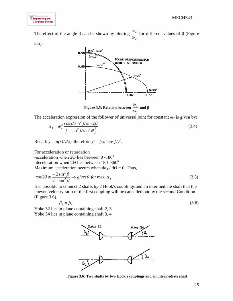
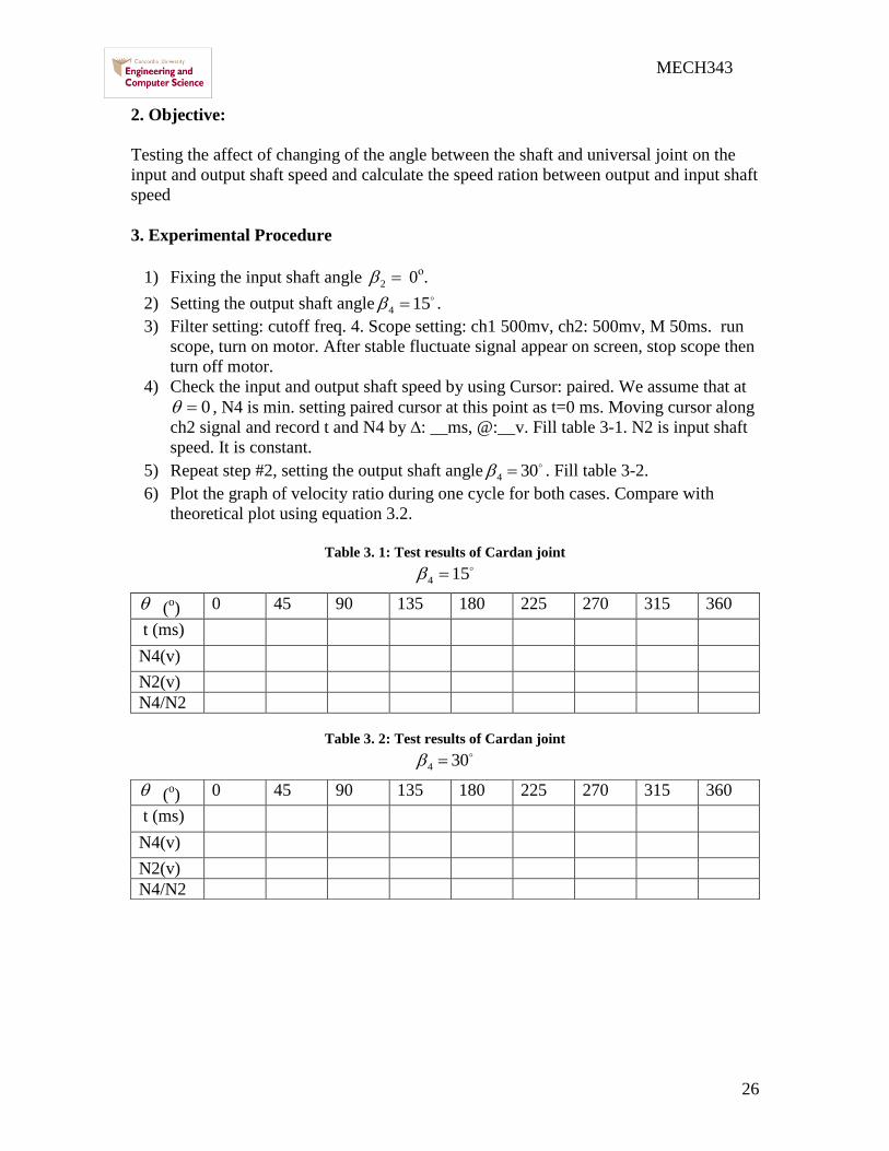
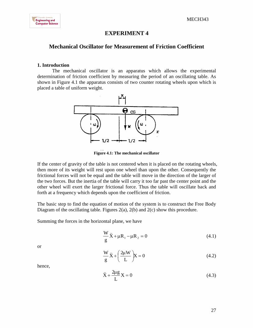
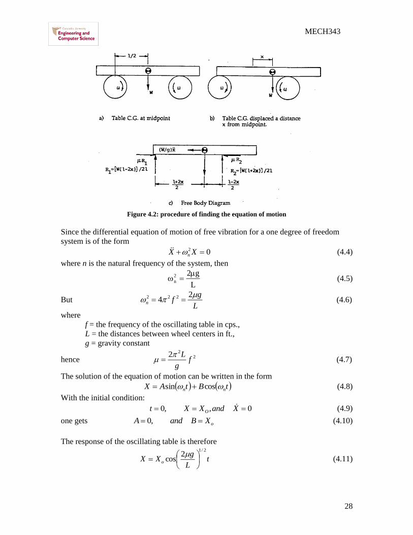
28
MECH343
Figure 42 procedure of finding the equation of motion
Since the differential equation of motion of free vibration for a one degree of freedom
system is of the form
02 XX n (44)
where n is the natural frequency of the system then
L
g22
n
(45)
But L
gfn
24 222 (46)
where
f = the frequency of the oscillating table in cps
L = the distances between wheel centers in ft
g = gravity constant
hence 2
22f
g
L (47)
The solution of the equation of motion can be written in the form
tBtAX nn cossin (48)
With the initial condition
00 XandXXt O (49)
one gets oXBandA 0 (410)
The response of the oscillating table is therefore
tL
gXX o
212
cos
(411)
29
MECH343
tL
g
L
gXX o
21212
sin2
(412)
tL
g
L
gXX o
212
cos2
(413)
Thus it may be concluded that the response of the oscillating table is governed by the
initial displacement X0 the coefficient of friction micro and the difference between wheel
centers L
2 Objectives
The experiment is designed to illustrate some of the direct applications of the
theory of vibration to the measurement of physical quantities The experiment also
demonstrates the differences between mathematical models and actual physical systems
Calculate the friction coefficient between the wheels and the bars
3 Description of Experiment
The oscillating table apparatus consists of four grooved wheels mounted on two
axels which are driven by a 120 HP electric motor and a gear reduction unit in opposite
directions The table consists of circular rods connected in a rectangular shape such that
the rods are guided by the grooved wheels
4 Experimental Procedure
1) Measure L the length between the centers of the two wheels
2) Locate one of the bars on the wheels
3) Select two different speeds for the wheels and when it starts rotating and the bar
moving calculate the time for 10 oscillations
4) Calculate the experimental coefficient of friction μ through the following
equation 2
22f
g
L When f is the frequency g gravity acceleration L the
length between the centers of the two wheels Fill table 4-1
5) Find the theoretical coefficient of friction μ for all bars
6) Compare between theoretical and experimental coefficient of frictions μ
Table 4 1 Combinations for measuring the friction coefficient
Case Material of
the bar
Speed
(rpm)
Time taken
for 10
oscillation
Frequency
(f)
Coefficient
of friction
(micro)
Standard
coefficient
of friction
1 Steel
2 Brass
3 Aluminum
30
MECH343
EXPERIMENT 5
5-1 PLANETARY GEAR TRAIN KINEMATICS
1 Introduction
A planetary gear train is one in which the axis of some of the gears may have motion A
planetary gear set always includes a sun gear one or more planet gears and a planet
carrier or arm which sometimes called as sun-and-planet planetary gear train as shown in
Figure1
Figure 51 Planetary gear train
A planetary gear set as shown in Figure 52 is one having two degrees of freedom This
means that the motion of each and every element of the mechanism is not defined unless
the motion of two of its elements is specified To make the planetary set a one degree of
freedom gear train one must fix the motion of one element of the mechanism
Figure 52 Sun-and-planet planetary gear train
2 Solution of Planetary Trains by Formula Methods
Figure 53 shows a planetary gear set which is composed of a sun gear 2 an arm 3 and
planet gears 4 and 5
31
MECH343
Figure 53 Compound Planetary Gear Set
We can express the velocity of gear 2 relative to the arm 3 in the form
3223 nnn (51)
3553 nnn (52)
Dividing Equation (52) by (51) gives
32
35
23
53
nn
nn
n
n
(53)
Since this ratio is the same and is proportional to the tooth numbers it is equivalent
therefore to the train value e
32
35
nn
nne
(54)
Or AF
AL
nn
nne
(55)
where nF = rpm of first gear in train
nL = rpm of last gear in train
nA = rpm of arm
The experiment is designed to demonstrate the fundamentals of planetary gear train and
to show all possible motions that can be obtained with this type of gear trains
3 Objective
Calculate the gear train ratio for the planetary gearbox and the degrees of
freedom that the system has
4 Experimental Procedure
For the planetary gear trains mechanism shown in Figure 51
1) Calculate the degree of freedom to the planetary gear system
2) Calculate the gear train ration through the following equation
21
23
nn
nne
When the outer ring is fixed
When the planet gears are fixed
32
MECH343
5-2 The Borg-Warner Model 35 Automatic Transmission
Simulator
1 Introduction
The Borg-Warner Model 35 Automatic Transmission comprises a three element
torque converter--coupling and a planetary gear set to provide three forward ratios and
reverse
The planetary gear set consists of two sun gears two sets of pinions a pinion
carrier and a ring gear
Power enters the gear set via the sun gears In all forward ratios power enters
through the forward sun gear In reverse it enters through the reverse sun gear Power
leaves the gear set by the ring gear and the pinions are used to transmit power from the
sun gears to the ring gear
In reverse a single set of pinions is used which causes the ring gear to rotate in the
opposite direction from the sun gear In forward ratios a double set of pinions is used to
cause the ring gear to rotate in the same direction as the sun gear
The Carrier locates the pinions relative to the two sun gears and the ring gear also
forming a reaction member for certain conditions The various mechanical ratios of the
gear ser are obtained by the engagement of hydraulically operated multi-disc clutches and
brake bands
Power flow in each ratio is achieved by locking various elements of the planetary gear set
as follows
1st Gear (Lockup selected)
The front clutch is applied connecting the converter turbine to the forward sun
gear The rear band is also applied holding the pinion carrier stationary The gear set
provides the reduction of 239 l The reverse sun gear rotates freely in the opposite
direction to the forward sun gear
33
MECH343
1st Gear (Drive selected)
The front clutch is applied connecting the converter turbine to the forward sun
gear The one-way clutch is in operation preventing the pinion carrier from moving
opposite to the engine rotation The gear set again provides the reduction of 239 1 On
the overrun the one-way clutch unlocks and the gear set freewheels
2nd Gear (Lockup or drive selected)
Again the front clutch is applied connecting the converter turbine to the forward
sun gear The front band is applied holding the reverse sun gear stationary The pinions
now walk around the stationary sun gear and the gear set provides the reduction of 145
l
3rd Gear (Drive selected)
Again the front clutch is applied connecting the converter turbine to the forward
sun gear The rear clutch is applied connecting the turbine also to the reverse sun gear
Thus both sun gears are locked together and the gear set rotates as a unit providing a
ratio of 1 1
Neutral and Park
The front and rear clutches are released and no power is transmitted from the
converter to the gear set
Reverse
The rear clutch is applied connecting the converter turbine to the reverse sun gear
The rear band is applied holding the pinion carrier stationary providing a reduction of
209 l
2 Gear Ratios
119866119890119886119903 119877119886119905119894119900 120579119900120579119894
=1
239
The carrier is held stationary to provide the
reaction member and the gears operate as a
Simple gear train
34
MECH343
The reverse sun gear is held to that the gears
now operate as an epicyclic gear train
For an epicyclic gear train shown as following
119866119890119886119903 119877119886119905119894119900 120579119900120579119894
=1
145
119894134 =
1205961 minus 1205964
1205963 minus 1205964= minus
11988521198851
11988531198852prime
119900119903 120596119871
32
67= 120596119869 minus 120596119871 120596119869 =
99
67120596119871
For our transmission show as above
119894119865119869119871 =
120596119865minus120596119871
120596119869minus120596119871= minus
119885119866
119885119865
119885119867
119885119866
119885119869
119885119867=
67
28 (1)
119894119865119870119871 =
120596119865minus120596119871
120596119870minus120596119871= minus
119885119866
119885119865
119885119867
119885119866
119885119870
119885119867= minus
32
28 (2)
Hence minus120596119871
120596119869minus120596119871= minus
67
68
28
32
From (2) 120596119865 minus 120596119871 =32
28 120596119871 120596119865 =
60
28120596119871
Therefore 119894119865119869 =120596119865
120596119869=
60
28
67
99= 145021645
So 120579119900
120579119894=
1
145
35
MECH343
119866119890119886119903 119877119886119905119894119900 120579119900120579119894
=1
1
Both sun gears are locked together and the
gears set rotates as a unit
119866119890119886119903 119877119886119905119894119900 120579119900120579119894
=1
209
With the reverse gear engaged power is
applied to the reverse sun gear The planet
carrier is held stationary so that the planet
gears rotate the ring gear in the opposite
direction to the reverse sun gear
36
MECH343
3 Experimental Procedure
Pins and slotted plates represent the multi-disc clutches and brake bands The various
gear ratios of the gear set may be obtained by inserting the appropriate pins as indicated
below
A B C D E F
Lockup 1Drive 1
Lockup 2Drive 2
Drive 3
Reverse
Neutral
Park Note
1 Lose all pin and turn input shaft and output shaft make sure input shaft disk and
output shaft disk indicate to 0 then lock pins for each case
2 Turn input shaft one turn (360 ) read output disk (degree)
3 Fill out following table
Input (degree) Output (degree)
Lockup 1Drive 1 360
Lockup 2Drive 2 360
Drive 3 360
Reverse 360
4 Results
According to power flow and gear ratio figures for each case referring to 2nd gear
ratio calculation derive and calculate gear ratios for 1st 3
rd and reverse shift Compare
them with your experimental results
37
MECH343
EXPERIMENT 6
Static and Dynamic Balancing
1 Objective
The objectives of this experiment are
Understanding the concept of static and dynamic balancing
Understanding unbalance torque
Justifying theoretical calculation for balancing with experiment
Balancing the shaft by the four given masses
2 Introduction
Unbalanced dynamic forces effects have profound influence on the working and
of rotating machinery like turbines compressors pumps motors etc These forces act
directly on the bearings supporting the rotor and thus increase the loads and accelerate the
fatigue failure These unbalanced forces induce further mechanical vibrations in the
machinery and connected parts thereby creating environmental noise problem through
radiation of sound Hence it is desirable to balance all such uncompensated masses and
thus reduce the effect of unbalance forces in a dynamics balancing machine
Balancing is the technique of correcting or eliminating unwanted inertia forces which
cause vibrations which at high speeds may reach a dangerous level An important
requirement of all rotating machinery parts is that the rotation axis coincides with one of
the principal axis of inertia of the body After a roll is manufactured it must be balanced
to satisfy this requirement especially for high speed machines The condition of
unbalance of a rotating body may be classified as static or dynamic unbalance
2 1 Static Unbalance
An idler roll is statically balanced if the roll doesnt rotate to a heavy side when free to
turn on its bearings Thus the rolls center of gravity is on the axis of rotation Static
unbalance (Figure 61) creates a centrifugal force when rotating which causes deflection
of the roll Idler rolls are sometimes static
balanced only when the roll operates at slow
speeds
The static unbalance usually happens because
of errors in the manufacturing tolerances of
the rotating parts Therefore static imbalance
is essentially a weighing process in which the
part is acted upon by either gravitational or
centrifugal force This type of unbalance
could be easily reduced or removed by static
balancing
Figure 61 Static (or force) Unbalance
38
MECH343
2 2 Dynamic Unbalance
An idler roll may be in perfect static balance and not be in a balanced state when rotating
at high speeds A dynamic unbalance is a ldquocouplerdquo or twisting force in two separate
planes 180 degrees opposite each other (Figure 62) Because these forces are in
separate planes they cause a rocking motion from end to end A roll that is unbalanced
will cause 1) machinery vibrations 2) web
flutter and 3) a decrease in bearing life due to
unnecessary forces
To dynamically balance a roll it must first be
statically balanced Then the roll must be
rotated to its operating speed and have the
dynamic unbalance eliminated by adding or
subtracting weight The determination of the
magnitude and angular position of the
unbalance is the task of the balancing
machine and its operator Balancing
machines are provided with elastically
supported bearings in which the idler roll may
spin Because of the unbalance the bearings
will oscillate laterally and the amplitude and
phase of the roll are indicated by electrical
pickups and a strobe light
Figure 63 shows a long rotor which is to be mounted in bearing A and B We might
suppose that two equal masses m1 and m2 are placed at opposite ends of the rotor and at
equal distances r1 and r2 from the axis of rotation Since masses are equal on opposite
sides of the rotational axis the rotor is statically balanced in all angular positions But if
the rotor is caused to rotate at an angular velocity ω radsec the centrifugal forces m1r1ω2
and m2r2ω2 act respectively at m1 and m2 on the rotor ends These centrifugal forces
produce the equal but opposite bearing reactions FA and FB and the entire system of
forces rotate with the rotor at the angular velocity ω Thus the rotor is to be statically
balanced and at the same time dynamically unbalanced
Figure 63 Dynamically Unbalanced Rotor
Figure 62 Dynamic (or couple) Unbalance
39
MECH343
3 Principle and Theory of Operation
Consider a body of mass M rotating with a uniform angular velocity about O with
eccentricity e as shown in Figure 64 The centrifugal force Fc acting on the axis of
rotation is Me2 This force is therefore very sensitive to speed and hence there is a need
to reduce this force either by operating at lower speeds or by decreasing the eccentricity
as shown in Figure 65
O
e
M
M e
2
Figure 64 Unbalanced Disc
Center of rotation
( new center of
gravity )
Rotating Disc Added mass m
Center of gravityOriginal center
of gravity
(a) (b)
Figure 65 Illustration of The Simplest Method of Static Balancing
In general it is desirable to make e as low as possible If the rotor thickness to diameter
ratio is less than 05 and speed are below 1000 rpm the rotor can be single plane
balanced - otherwise two-plane balancing is necessary In the single plane balancing
technique with a rotor of mass mi and radius ri from the axis of rotation and lying in the
same plane the condition for static balance is used
0~iirm (61)
where i = 1 2 which denotes the total number of masses and m denotes the mass The
vector ir~ represents the eccentricity e of the mass mi from the axis of rotation
When the bodies are rotating in several planes the condition for dynamic balance has to
be satisfied in addition to that for static balance This is given by
0~~ iii rzm (62)
where iz~ is the axial coordinate vector of the mass mi measured for a chosen datum In
the two-plane balancing technique instead of satisfying Equations (61) and (62)
40
MECH343
explicitly Equation (62) is used with two different datum planes for iz~ Mathematically
if the distance between these two plane is oz~ then
0~)~~( ioii rzzm (63)
It is therefore clear that Equations (62) and (63) imply the satisfaction of Equation
(61) Conceptually it means that if a system of bodies rotating in several planes is in
dynamic balance with respect to two different datum planes then the system is also in
static balance This is the principle of the two-plane balancing technique
4 Description of Experimental Apparatus
Figure 66 shows the Static and Dynamic Balancing Apparatus It consists of a perfectly
balanced shaft with four rectangular blocks clamped to it The shaft is mounted in ball
bearings and it is driven by a 12 volt electric motor through a belt and pulley drive The
shaft assembly is mounted on a metal plate resting on four resilient rubber supports
which allow the mount to vibrate when the shaft is not balanced
The rectangular blocks can be clamped to the shaft at desired out-of-balance moments by
means of discs having eccentric holes of various diameters The discs are fixed to the
blocks by hexagon socket set screws Any longitudinal and angular position of a block
relative to the shaft can be set by linear and protractor scales provided Adjacent to the
linear scale is a slider which can be pushed against the block to read its longitudinal
position The slider also serves as a datum stop against which the blocks can be held
when reading their angular position on the shaft
The out-of-balance moments are measured by fitting the extension shaft and pulley to the
main shaft Each rectangular block is then clamped to the shaft in succession A cord with
a weight bucket at each end is hung on the pulley and bearing balls are placed in the
bucket until the block has turned through 90deg The out-of-balance moment is proportional
to the number of balls required
to turn the block
A Perspex dome serves as the
safety cover The shaft cannot
be driven unless the dome is in
position which is achieved by
micro switches actuated by the
dome The motor switch on the
front panel is spring loaded so
that the motor cannot be left
running The motor requires a
power supply of 12 volts at 2
amperes which is provided by
E66E90 speed controller
Figure 66 Static and Dynamic Balancing Apparatus
41
MECH343
5 Experimental Procedure
5 1 TEST 1 Static Balancing
1 Looking at the shaft from the side the masses will be as shown in figure 6-7
each mass has an angle θ with horizontal
Figure 6-7 Shaft view from the side
2 The masses forces are given by the following table 6-1
The masses values Table 6-1
3 In order to balance the shaft statically the sum of the forces will be equal zero
as the following equations
sum F=0
F1cos θ1+ F2cos θ2+ F3cos θ3+ F4cos θ4=0 (1)
F1sin θ1+ F2 sin θ2+ F3 sin θ3+ F4 sin θ4=0 (2)
4 Since we have just two equations with four unknown angles we assume
θ1=0ordm θ2=90ordm
5 Solving the two equations or using force polygon by AutoCAD to find the θ3
θ4
5 2 TEST 2 Dynamic balancing
1 Looking for the shaft from in front the masses create the forces as shown in
figure 6-8 each mass has an arm X create a momentum
F1
F2
F3
F4
42
MECH343
2 In order to balance the shaft dynamically the sum of the momentum will be
equal zero as the following equations
sum M=0
F1cos θ1X1+ F2cos θ2X2+ F3cos θ3X3+ F4cos θ4X4=0 (1)
F1sin θ1X1+ F2 sin θ2X2+ F3 sin θ3X3+ F4 sin θ4X4=0 (2)
3 Since we have just two equations with four unknown arms we assume
X1=50 mm X2=100 mm
4 Solving the two equations or using momentum polygon by AutoCAD to find
the X3 X 4
TABLE 6 2
Block 1 2 3 4
Mass 88 82 74 64
Angle θ(ordm) 0 90
Arm X (mm) 50 100
6 Typical Calculations
The basic equations that are used for balancing purposes are
0rW ii (63)
0rWa iii (64)
Suppose that block (1) is placed 17 mm from the left end of the shaft at zero angular displacement and that
block (2) is placed 100 mm from it at 120deg The measured out-of-balance moments are as follows
Figure 68 In front shaft view
43
MECH343
TABLE 6 3 OUT-OF-BALANCE MOMENTS
It is first necessary to draw the moment polygon of Wr values as shown in Figure 68 to determine the
angular positions of blocks (3) and (4) W1r1 and W2r2 are known in both magnitude and direction The
vector W1r1 has been drawn at positive X-direction (θ = 0) The lengths of vectors W3r3 and W4r4 are known
and arcs can be drawn from the ends of W1r1 and W2r2 to get the directions of the unknown vectors
Figure 69 shows the diagram of the angular positions and the corresponding longitudinal locations of the
blocks on the shaft are 17 mm for the first 117 mm for the second block
To find the longitudinal positions of the other two blocks we designate distance of block (3) by a3 and
distance of block (4) by a4 measured from block (1) so block (1) is the reference and will not appear in
calculations
Draw a vector a2W2r2 = 100 (82) units long parallel to r2 and vectors a3W3r3 and a4W4r4 parallel to r3 and r4
respectively so that the moment polygon is closed The lengths of vectors a3W3r3 and a4W4r4 can be
measured and the magnitudes found by using the scale factor From these a3 and a4 can be calculated
Notice that the sense of vector a3W3r3 is reverse In order to maintain vector a3W3r3 the only possible
solution is to reverse a3 So from the vector polygon (triangle) it follows
a3 = -12 mm
a4 = 124 mm
This means that block (3) should be located 5 mm from the left end of the shaft The blocks should be
positioned as follows
Block Angular Position (Deg) Longitudinal Position (mm)
(1) 0 17
(2) 120 117
(3) 190 5
(4) 294 141
The values of a3 and a4 can be found analytically using complex vector approach
Real and imaginary components yield
100(82) cos 120deg + (74) a3 cos 190deg + (64) a4 cos 294deg = 0
100(82) sin 120deg + (74) a3 sin 190deg + (64) a4 sin 294 deg = 0
which reduce to
4100- 7288 a3 -2603 a4 = 0
71014- 1285a3 -5847 a4 = 0
44
MECH343
Solving the two equations gives a3 = -1194mm a4 = 12396mm
The values compare very well with those obtained graphically
In order to obtain independent results it is suggested that Wr values of the blocks are varied by using
different positions of the discs with eccentric holes The angular displacements between blocks (1) and (2)
may also be varied
Figure 69 Moment Polygon of Wr
45
MECH343
EXPERIMENT 7
Machine Fault Simulator (MFS)
1 Theory
Refer to experiment number 6
2 Description of Experimental Apparatus
Figure 71 shows the machine fault simulator The rotor is driven by a variable speed
motor via a flat belt and the rotor rotational speed is captured through a digital
tachometer The vibration due to the unbalanced rotor is measured and fed directly into
the on-board processor of the machine
Figure 71 Machine Fault Simulator
3 Objective
In this experiment we will study the reaction of the shaft and the motor when the shaft is
balanced and when it is unbalanced
4 Experimental Procedure
1) Run the Vibro-Quest Software
o Define a ldquoNew Projectrdquo (under root)
o Fill up the window select ldquoProject namerdquo click ldquoNextrdquo
o Select ldquoNonerdquo from the menu on the right side click ldquoNextrdquo
Belt
Motor
Disk A Disk B
Reciprocating
Mechanism
Speed
Control
46
MECH343
o Review the table (do not change the default) click ldquoNextrdquo
o Review the table check the setting data click ldquoNextrdquo
o Click ldquoDonerdquo
o Review the information provided if they are not ok ldquoGo backrdquo to modify
the data then click ldquoFinishrdquo
2 Select ldquoDatardquo from the toll bar on the computer
3 Name the ldquoTest Titlerdquo in the window Insert the parameters used in the test and
click ldquoNextrdquo
4 Review the information provided in the window and click ldquoNextrdquo
5 Chose 2000 as Frequency limit 1600 for Space line Leave the rest information as
defaulted and ldquoGO DAQrdquo
2) Running the Machine Fault Simulator
Select the required speed (rpm) change it to frequency (Hz) using the following
relation 60)rpm(n2)Hz(f
1 Run the machine using speed control system at desired speed
2 Wait about 15 seconds to stable the system
3 Click onrdquo START RECORDINGrdquo
4 When the recording is finished save the file under the root of ldquoDatardquo of base line
at the subdirectory that you want to compare with the other data (for example if
you are running the machine at 20 Hz save the your file under 20 Hz subdirectory)
5 Now select the ldquoProject namerdquo from the left menu all the relevant tests will
appear at the right table under the ldquoTest Explorerrdquo
6 To compare the data from different files Hold down the ldquoShiftrdquo key and select
any two interested files that you are going to compare
7 Click on ldquoComparerdquo to observe the difference between the unbalanced system
with a base system
8 To observe more clearly the difference between the frequency responses of the
different test click on ldquoOverlayrdquo
TEST 1 Imbalance Effects on Vibration response
Install the defined weight in one of the taped hole in rotor disk A and tight it
securely with a nut
Close the cover of MFS
Change the motor speed and record vibration level at each bearing For this
purpose you don not need to define new project for each speed define a new
project( follow steps 1-6 from section 3) then follow steps 1-2 for each speed
from section 4
Measure the average level of amplitude at each speed and Plot it against the speed
Repeat steps 2-5 for 2 different weights at 2 different radius and angles
47
MECH343
TEST 2 Balancing the Imbalance Rotor
Add weight at different radius and angles using the ldquosample calculationrdquo to
balance the rotor
If the rotor is balanced define a ldquoNew projectrdquo and follow steps 3-8 of Section 4
Fill Table 7 1
TABLE 7 1
Unbalance weight on disc A ____________ angular position _______________
Mass Added on disk B gr r (mm)
Amp baseAmp New
48
MECH343
EXPERIMENT 8
DETERMINATION OF SPUR GEAR EFFICIENCY
1 Objective
The main objective of the experiment is to determine the efficiency of the
Spur gear and worm gear unit
2 Introduction and theoretical background
21 Pinion gear
Two intermeshed toothed wheels make up a pinion gear This type of gear
permits a positive transmission of motion and torque Wheel pairs are available in
different shapes and shaft configurations Figure 1 explains the various types of gears and
their arrangements
Fig8 1 Various types of gear arrangements
22 Worm gear
A worm gear is a screw-type transmission unit whose axes generally intersect at
right angles The worm and wheel make contact on a straight line Normally the worm
has a cylindrical core and the wheel globoid toothing Units with a very high performance
49
MECH343
consist of a globoid worm and globoid wheel A worm gear with a cylindrical worm has
the following special features
High load capacity compared with spur gears due to linear contact
Low-noise operation and high absorption of vibrations
Wide transmission range down to low ilt110
High efficiency at high transmission ratios high efficiencies(η le 98 ) can be
achieved with very sophisticated designs under favorable operating conditions a
decrease in pitch angle (high transmission ratio) or speed is accompanied by a
corresponding decrease in efficiency (to η le 50 )
Self-locking operation
Smaller and lighter design compared with spur bevel gear units possessing high
transmission ratios
23 Basic definitions
Drive torque
The drive torque is the product of the force F and the lever arm l on which the
force acts
M = F X l (1)
M is in Nm F is in N and l in m
Drive power
The drive power of a rotating shaft is the product of the torque M and angular
frequency ω P = M X ω (2)
and 60
2 n (3)
P is in W n is in rpm
Efficiency
The efficiency is defined as the ratio between the output and input powers It has a
maximum theoretical value of 1
in
out
P
P (4)
where speed i
nn 1
2
50
MECH343
3 Experimental set-up
Figure 2 shows the complete view of the experimental set up
Fig8 2 Complete view of GUNT AT 200 experimental set up
The modules comprising the drive unit spur gear worm gear and magnetic
powder brake are mounted on a profile frame The DC shunt motor is designed for right-
hand and left-hand rotation The drive unit is electrically powered via control housing
The control unit adjusts the DC machinersquos speed via its armature voltage Its target speed
is set by means of a potentiometer on this housing Its actual speed is measured and
indicated by means of an inductive proximity switch and evaluation unit The speed is
51
MECH343
measured inductively by a contactless sensor disc and indicated by a digital display
element on the control unit Electronic thyristor speed control with I x R compensation
provides a high torsional rigidity The reaction torque exerted on the drive housing is
measured by means of a spring force meter connected to a lever arm
The transmission units consist of a 2-stage spur gear with transmission
ratio i = 135 and a single-stage worm gear with transmission ratio i = 14The
transmission torque can be determined on the drive side as well as the brake side To
facilitate adjustment of the brake torque the brake characteristic (current torque) is
recorded in a preliminary experiment Moments are determined through power
measurements (spring balance) with a known lever arm The moments measured input
speeds and transmission ratios are used to determine power and efficiency
The magnetic powder coupling consists of two independently mounted
rotors ie a primary and a secondary rotor both furnished with ball bearings The
primary rotor also serves as a coil carrier If one of these two rotors is deactivated the
magnetic powder coupling can also be used as a brake The air gap between the two
rotors contains a special magnetic powder If a direct voltage is applied to the excitation
winding the powder aligns itself with the resulting magnetic field lines to form a
compact mass providing a frictional link between the primary and secondary rotors The
value of the torque depends on the adjusted current When the current-proportional
moment is exceeded slippage occurs without any transition
4 Experiments procedure
As shown in Figure 82 the complete view of the experimental set up for this
experiment there is input as the motor speed and the output as excitation current so that
there is two steps for this experiment
After making sure spur gear is connected as shown in Figure 83
1) Fix the output excitation current at I= 50 mA and change the speed of the motor as
shown in the table (1) each time measure the motor force F1 and the brake force F2
52
MECH343
Figure 83 Configuration of spur gear unit experimental set up
Measurement data to determine the efficiency of Spur gear unit Table (1) I = 50mA
SlNo Motor speed
( n1 ) rpm
Motor holding
force ( F1 ) N
Brake holding force
( F2 ) N
Efficiency ( η )
1 500
2 1000
3 1500
4 2000
5 2500
In order to find out the spur gear efficiency we go through the following equations
The general equation for the spur gear efficiency is
in
out
P
P
The drive power of a rotating shaft is the product of the torque M and angular
frequency ω P = M X ω
The drive torque is the product of the force F and the lever arm l on which the
force acts
M = F Arm
When the arm for the motor Arm1=25 mm and for the brake Arm2=50 mm
53
MECH343
And the angular velocity from the following equation
60
2 n
In order to find the speed for the brake we use this ratio assuming i= 135
i
nn 1
2
2) Fixing the input n1= 1500 rpm and changing the output and filling table (2)
Recorded values of the excitation current and the force on the lever arm table (2)
Speed n1= 1500 rpm
Excitation current I (mA) Force F2 on the lever arm (N)
50
70
90
110
130
150
130
110
90
70
50
5 Experiments Results
1) Plot the characteristics curve between the current I and the force on the lever arm
F2
2) Plot the characteristics curve between the current I and the torque M
3) Determine the efficiency of the spur gear unit Comment on the errors on the
efficiency if the calculated efficiency deviates from the realistic values of 80 -
90
54
MECH343
EXPERIMENT 9
ANALYSIS OF LINKAGE MECHANISM
Try to build a linkage mechanism as the figure below
Steps
1 Turn on grid line from View-workspace-grid lines as below
2 Select rectangle tool
55
MECH343
3 Click and drag a small rectangle
4 Click the rectangle copy it (CTRL+C) paste it (CTRL+V) two times
5 Change the length of each rectangle by selecting it and writing down the desired
length in the text box named W
Make the length as (3 ndash 332 - 4)
56
MECH343
6 Use the rotate tool and the select tool to arrange the rectangles
Make sure that the spacing is 4 units as shown below
7 Put a motor at the lower end of the left link
- First select the motor - Then click at the desired point
57
MECH343
8 Put a pin joint at the lower end of the right link
- First select the pin joint - Then click at the desired point
9 Put a point element at the remaining ends
- First double click (this
enable you to assign multiple
points) on the point element
It should look like below
58
MECH343
10 Join the links by selecting two points then selecting Join
Click the arrow select tool
Select first point ndash
press SHIFT and
click the other point
Press
Join
They should look like
below
11 Repeat the same for the remaining two points Your model should look like below
59
MECH343
12 Click RUN ( ) and watch it rotating
13 Now we want to capture the velocity of the joint between the left link and the middle
one
- Select it and click on Define ndash Vectors-
Velocity
Click Run and watch the velocity change
Note that by clicking on the link itself and defining the velocity the program calculates
the velocity of the CG of the link
14 Now you are ready to try different measurements
Acceleration Total Force Gravitational Force
60
MECH343
15 Select a link and use the measure tool
X- Position Graph
Y- Position Graph
61
MECH343
Measuring velocity values
16 Now try to change the length of any of the links and RUN the model and observe
for any change if any and explain
17 Change the mass of any of the links and observe for any change in velocity and
force And Why if there is any
18 Now double click on the motor (resetting the mass for any link that has been
changed) and notice that the value for velocity is 1 radsec Change this to make it the
same value for acceleration and torque Write what you observe and try to explain
19 Now increase the mass for one link (eg left one) gradual and see how this will
affect the motion for a fixed value for torque velocity or acceleration of the motor
20 Now replace the middle link with two links connected with total length as the
middle one run observe and explain
21 Based on (20) search for what is the equation relation or rule that governs the
mechanism motion
62
MECH343
EXPERIMENT 10
NUMERICAL DYNAMIC SIMULATION FLYWHEEL
Problem Definition
In the two cycle piston engine shown explosive gases are
ignited in the combustion chamber above the piston The
explosions apply a force of 150 N for the duration of every
downward stroke The engine is equipped with a speed
limiting device (rev limiter) which prevents the rotational
speed from exceeding a set value (red-line) The masses of
the piston and connecting rod are 075 kg and 15 kg
respectively The mass of the crankshaft-flywheel assembly
is 30 kg Given that the red-line of the engine is 35 radsec
(340 rpm) Assume the crankshaft-flywheel assembly can
be modeled as a circular disk
Objective
Determine the forces at the crankshaft bearing (point A) and connection rod (point B)
bearing
Solution
1 INTRODUCTION
Engines that exceed the manufacturers maximum speed (over-revving) may be subject to
excessive wear and possible failure To prevent over revving internal combustion
engines are often fitted with a device known as a rev-limiter When an engine exceeds its
red-line rev-limiters interrupt the ignition system slowing the engine down Once the
speed drops below the maximum the ignition system is switched back on In this exercise
you will model an internal combustion engine equipped with a rev-limiter The engine
has three bodies the piston the connecting rod and the crankshaft The piston will be
modeled by a square body The connecting rod will be modeled by a rectangular body
The crankshaft will be modeled as a circular body The bodies will be drawn sized and
joined to each other and the background The pistons cylinder walls will be modeled with
a keyed slot joint The force of combustion will be modeled by a force attached to the top
of the piston The resulting forces at the bearings will be measured
2 SETTING UP THE WORKSPACE
For this exercise three changes in the workspace will be made First for clarity the x-y
axes will be displayed The unit of distance will also be changed from meters (default) to
millimeters
63
MECH343
If the x-y axes are not currently displayed choose Workspace from the
View menu and choose XY Axes from the Workspace submenu The x-y
axes provide a reference frame for building a simulation
Choose Numbers and Unitshellip from the View menu The Numbers and
Units dialog appears
Click the More Choices button The dialog box expands
Click and hold in the Distance field (Figure 1) The pop-up menu appears
Choose millimeters from the Distance pop-up menu
Click in the Rotation field and choose Radians from the pop-up menu
Click OK
3 CREATING THE COMPONENTS
This exercise has three objects a 15 kg connecting rod a 075 kg piston and a 30 kg
crankshaft (see Figure 2 below) The connecting rod will be modeled by a thin rectangle
400 mm in length Its width will be thin 150 mm so it closely resembles the actual
connecting rod The crankshaft as stated in the exercise is modeled as a circular disk
with a 200 mm radius and a mass of 30 kg A 200 mm square object will represent the
piston The objects will be created sized and initialized in the following steps
Creating the Crankshaft
The crankshaft is represented by a circle with a radius of 200 mm and mass of 30 kg
These parameters will be set using the Geometry and Properties utility windows
I To draw the crankshaft
64
MECH343
bull Click the Circle tool in the Toolbar
bull Click once on the background Move the mouse to expand the circle and click
again to complete sketching
II To set the mass of the crankshaft
Choose Properties from the Window menu
Click the mass field and enter the value 30
III To set the size of the crankshaft
Select the crankshaft if it not already selected
Click the Radius field (labeled ldquorrdquo) of the Coordinates bar and enter the value 200
(Figure 3)
IV Zooming In
The circle will appear small after sizing To make the rectangle easier to manipulate and
appear larger the workspace will be magnified using the Zoom tool To zoom in
Click the Zoom In tool in the Toolbar
Click near the circle The objects in the window are magnified by a factor of two with
each click of the mouse To zoom out while the Zoom In tool is selected hold down
65
MECH343
the Shift key (the magnifying glass pointer changes to ldquo-rdquo) and click Your screen
should be similar to Figure 4 below
Figure 4 The workspace after zooming in
Click the Arrow tool in the Toolbar or press the spacebar to deselect the Zoom In
tool
Creating the Piston
For this exercise the piston will be modeled as a 200 mm square with the mass of 75 kg
The Square tool will be used to draw the piston and the Properties window will be used
to set its mass
I To draw the piston
Choose the Square tool in the Toolbar On systems the Square tool is ldquohiddenrdquo in the
RectangleSquare pop-up palette by default Click and hold on the Rectangle tool to
bring the pop-up palette in view (Figure 5 below)
Click once on the background drag to the right and click again to complete
sketching A square appears on the screen To set the size of the piston
Click in the Height or Width field of the Coordinates bar and enter 200 Either field
changes both the height and the width of the object so that it remains square
Figure 5 RectangleSquare pop-up palette
II To set the pistonrsquos mass
bull Select the piston if it not already selected
bull Choose Properties from the Window menu
66
MECH343
bull Click in the mass field and enter the value 075
Creating the Connecting Rod
In this exercise the connecting rod is represented by a rectangle drawn with the
Rectangle tool and sized using the Geometry window To approximate an actual
connecting rod the rectangle will be given a mass of 2 kg a height of 500 mm and a
width of 100 mm
To draw the connecting rod
I Choose the Rectangle tool in the Toolbar (On systems the Square tool used above
may have replaced the Rectangle tool in the Toolbar If so the Rectangle tool may be
selected from the hidden pop-up palette by clicking and holding on the Square tool in
the Toolbar)
II Click once on the background drag to the right and click again to complete
sketching A rectangle appears on the screen To set the mass of the connecting rod
bull Select the new rectangle if it not already selected
bull Choose Properties from the Window menu
bull Click in the Mass field and enter the value 2
To set the size of the rod
1 Click the Height field of the Coordinates bar and enter the value 500
2 Click the Width field of the Coordinates bar and enter the value 100 Your screen
should resemble Figure 6
Figure 6 The piston crankshaft and connecting rod
Creating the Points for Joining
The objects in this exercise are connected to each other and to the background (see Figure
7 below) The connections will be modeled by creating points and joining them These
points will be created with the Point tool and accurately positioned using the Properties
window
67
MECH343
Figure 7 The points which will be created and their coordinates
Creating Points on the Connecting Rod
Double-click the Point tool in the Toolbar Double-clicking selects a tool for
successive operations On systems the difference between single and double-clicking
is indicated in the Toolbar by shading a doubleclicked item is dark grey while a
single-clicked item is light grey
Place the mouse pointer over the connecting rod rectangle Find the snap point at the
top end of the connecting rod An X symbol appears at snap points Find the snap
point located at the midpoint of the top side of the connecting rod
To attach a point element click when the snap point located at the top end is visible
Observe that the point element is attached to the top end of the rod
In the same fashion attach another point element to the bottom end of the connecting
rod Your screen should resemble Figure 8
Figure 8 Connecting rod points in position
68
MECH343
Attaching Points to the Crankshaft
The crankshaft needs two points a center point representing the main bearing and an
outer point representing the connecting rod bearing These points will be accurately
positioned at the center and at 200 mm from the center of the circle To create and
position the crankshaft points
Make sure the Point tool is still selected Place the mouse pointer over the
crankshaft Find the snap point at the center of the circle
Click when the snap point at the center is visible A point element is attached to
the center of the circle
Place the mouse pointer near the left quadrant of the circle Find the snap point at
the left quadrant (Figure 9) As the mouse pointer nears the left quadrant of the
circle the snap point appears
Click when the snap point at the left quadrant is visible Another point element is
attached to the left quadrant of the circle
Figure 9 Snap point at the left quadrant of the circle
Attaching Points to the Piston
Two points need to be attached to the piston a square point and a point The square point
will be joined to the slot on the background to create a keyed slot joint The point will be
joined to another point on the connecting rod to form a pin joint The square point will be
positioned on the piston at the coordinates of (0 -50) The square point will be rotated 90deg
so that when joined to the slot the piston will not rotate This is because vertical slots are
defined as being rotated 90deg horizontal slots are defined as having 0deg rotation When a
square point is joined to a slot the rotations of the two objects are aligned
I The point will be positioned at (0 0) To create the points
Click the Square Point tool The cursor turns into a square point
Click anywhere on the piston Since the square point will be precisely position
using the Coordinates bar below it is not necessary to find a snap point
Click in the X field of the Coordinates bar and enter 0 If you attached the square
point on a snap point the x-field of the Coordinates bar may contain a formula
expression (such as body[3] width or (00)) Simply overwrite the entire
expression and enter 0
Press the tab key to move to the Y field of the Coordinates bar and enter -50
Again simply overwrite the y-field with the value -50
Choose the Properties in the Window menu The Properties window appears
In the angle field of the Properties window (marked by oslash) enter the value 1571
The value of 1571 radians is equivalent to 90deg The value will be displayed in a
69
MECH343
rounded form but internally the correct value will be used The pointrsquos y-position
is set to -50 so it will not interfere with the connecting rod joint
II To create the point
Click the Point tool
Place the pointer near the center of the square and find the snap point
Click when the snap point at the center is visible The point is created at the center
of the piston
Attaching a Point to the Background
A point representing the main bearing of the crankshaft must be placed on the
background The point can be placed anywhere on the background for clarity it will be
placed at the origin (0 0) To create and position the point
Click the Point tool
Place the mouse pointer near the origin Find the snap point that appears at the
origin Make sure that nobody is obstructing the origin The snap point does not
appear if the origin is covered by a body
Click when the snap point at the origin is visible Verify the position of the point
by noting the (x y) position in the Coordinates bar it should be (0 0) We now
name this point element so that it becomes easier to select later
Choose Appearance from the Window menu The Appearance window appears
In the name field (where it says Point) type Base Pin Since we will not be
needing the Appearance window for the rest of the exercise close the window by
(Windows) clicking the box marked ldquoXrdquo at the top-right corner of the window or
() clicking the box at the top-left corner of the window
Attaching a Slot to the Background
The cylinder walls of the engine will be modeled with a keyed slot joint The joint will be
made by joining the square point on the piston to a slot attached to the background The
slot can be located anywhere on the background as long as it is located on the
crankshaftrsquos centerline (the yaxis for this model)
To create and position the slot on the background
Choose the Vertical Slot tool in the Toolbar On systems the Vertical Slot tool
may be ldquohiddenrdquo in the Slot pop-up palette Click and hold on the Slot tool in the
Toolbar to bring the pop-up palette in view
Place the pointer near the point element attached to the origin Find the snap
point
Click when the snap point is visible A vertical slot appears
Creating Joints
In this exercise there are four joints (see Figure 10) The joints will connect the piston to
the slot the piston to the connecting rod the connecting rod to the crankshaft and the
crankshaft to the main bearing
70
MECH343
Figure 10 The points which will be joined
The following steps will demonstrate how to make these joints
I Joining the Piston to the Slot
In this example the piston slides in a cylinder The
cylinder will be modeled as a keyed slot joint The joint
is created by joining the square point on the piston to the
slot To create the keyed slot joint
Select the square point on the piston and while
holding down the Shift key select the slot The word
ldquoJoinrdquo of the Join button in the Toolbar changes
from gray to black indicating the two points can be
joined
Click the Join button in the Toolbar The piston
moves to the slot (see Figure 11) Joining the
Crankshaft to the Point on the Background The
crankshaft main bearing is modeled as a pin joint
The pin joint will be created by joining the point at
the center of the circle to the point at the origin
II To join the crankshaft to the origin
Choose Properties in the Window menu
From the selection pop-up menu located at the top of the
Properties window choose Base Pin (Figure 12) The
Base Pin is now selected
Hold the Shift key down and select the center point on
the crankshaft circle
Click the Join button The crankshaft circle moves to the
origin
To see how the circle representing the crankshaft is
constrained bring the mouse pointer over the circle hold
down the mouse button and drag the circle The circle
can rotate but is fixed to the Base Pin
Figure 11 Piston joined to the slot
Figure 12 Selecting an object in
the Properties window
71
MECH343
III Joining the Components
The piston connecting rod and crankshaft will now be joined together (see Figure
13) The following steps describe how to join them
Figure 13 Joining the components
IV To join the piston to the connecting rod
Select the (round) point on the piston and while holding
the Shift key down select the top point on the
connecting rod
Click the Join button The two objects will come
together
V To join the connecting rod to the crankshaft
Select the bottom point on the connecting rod and while
holding the Shift key down select the remaining (left)
point on the crankshaft
Click the Join button Your screen should resemble
Figure 14
Editing the collision property of a pair of bodies
The Smart Editor keeps joints together during editing To see this try dragging the
connecting rod The connecting rod will stay joined while it is dragged and the crankshaft
and piston will move accordingly When you are done dragging the rod move it back to
the approximate position shown in the problem description on the first page of this
exercise
Preventing a Collision
In Working Model objects which are directly connected to each other never collide
Notice that the piston and crankshaft may overlap when they are dragged during editing
Since the two objects are not directly connected they will collide when you run the
simulation To prevent the collision the Do Not Collide command will be used
To prevent a collision
Select the piston and while holding the Shift key down select the crankshaft
Figure 14 the completed engine
72
MECH343
Click and hold on the Object menu title in the menu bar (Figure 15) Notice that
there is a checkmark beside ldquoColliderdquo indicating that the pair of selected objects
will collide when you run the simulation
Choose Do Not Collide in the Object menu
Figure 15 Editing the collision property of a pair of bodies
Creating the Force
A 100 N force is applied at the top of the piston in the negative y-direction (down) The
force is only active while the piston is traveling with a negative y velocity The force will
be drawn using the Force tool and its magnitude and location will be set using the
Properties window
Drawing the Force
The force will be drawn in the downward direction using the
Force tool
To draw the force
Click the Force tool in the Toolbar
Place the pointer near the midpoint of the top end of
the piston Find the snap point
Click when the snap point is visible drag the mouse
upward and click again to create the force A force
attached to the piston appears (Figure 16) Do not be
concerned with the exact direction or magnitude of the
force for now
Sizing the Force
The forcersquos magnitude and direction will be set using the Coordinates bar To size the
force
bull Click the force vector to select the force
bull Click the Fy field of the Coordinates bar and type -100
bull Click the Fx field of the Coordinates bar and type 0 The force vector changes in
length to reflect its new magnitude
Figure 16 Creating a Force
73
MECH343
Timing the Force
The ignition timing of the engine must be simulated The problem states that the force is
active only on the downward stroke (ie when the piston has a negative velocity) The
rev-limiter cuts off combustion when the rotational velocity is greater than 35
radianssecond To simulate these conditions the ldquoand (ab)rdquo function will be
incorporated with the following formulas
To determine when the piston has a negative velocity use the following formula
body[c]vy lt 0
where c is the pistons object id number To determine the pistonrsquos id number place the
cursor over the piston and read the Status bar
To determine when the enginersquos speed is greater than 35 rads use the following
formula
body[d]vr lt 35
where d is the crankshafts object id number Use the Status bar as above to determine the
crankshaftrsquos id number
The complete equation is
and (body[c]vy lt 0 body[d]vr lt 35)
The complete equation will be placed in the Active When field in the forcersquos Properties
window Gravity will provide the initial downward velocity to start the engine
To set the timing of the force
Select the force
Choose Properties from the Window menu
Click in the Active When field at the bottom of the Properties window On
Windows systems you must first un-check the Always button before clicking in
the Active When field
Type the following formula (see Figure 17)and(body [c]vy lt0body[d]vrlt 35)
where c and d are the object id numbers of the piston and crankshaft respectively
The forcersquos rev-limiter equation is designed for counter-clockwise (positive)
engine rotation It is important that the
engine be ldquostartedrdquo in a position similar to
the figure on the first page of this section
If you want a rev-limiter which works in
both directions try incorporating the abs()
function into the formula
You can increase the width of the ldquoActive
whenrdquo field to view the entire equation by
resizing the Properties window
The simulation is ready to run
Click the Run button in the Toolbar The engine runs A warning may appear if
you run the engine long enough you can ignore the warning for now
When you are ready to continue click the Reset button in the Toolbar
Figure 17 Active When field is in
the property window for a Force
74
MECH343
Measuring Properties from the Simulation
A graph in conjunction with a digital meter is a nice way to illustrate the rotational speed
of the enginersquos crankshaft Two digital meters will be used to display the forces on the
bearings Follow the steps below to create these output devices
Displaying a Graph
The angular velocity of the crankshaft will be
displayed by a graph To create the graph
Select the crankshaft circle Four squares
ldquohandlesrdquo will appear around the circle
indicating that the circle is selected
Choose Velocity from the Measure menu
and Rotation Graph from the Velocity
submenu A meter resembling Figure 18
appears
Displaying Digital Force Meters
To display the digital force meters
bull Select the crankshaft-main bearing joint (see Figure 19)
bull Choose Force from the Measure menu A digital meter appears
bull Repeat for the connecting rod-crankshaft joint (see Figure 19)
A second digital meter appears You may need to move the meters
To move the meters
bull Select a meter
bull Drag it to any position you wish
Your window should resemble Figure 20
Running the Simulation
Run the simulation Notice that the angular velocity increases until it reaches 30 rads
This is so because we have turned off the force above 30 rads just as a rev limiter t urns
off the ignition of an engine above a certain speed
Figure 18 A Velocity Graph
Figure 19 The Force to be measured Figure 20 The completed workspace
75
MECH343
Modifying the Graph Display
You may notice that the axis labels occlude the numeric labels along the tick marks of the
plot You can modify the display options using the Appearance window For example to
turn off axis labels so that the numeric labels clearly appear
Select the velocity meter on the screen
Choose Appearance in the Window menuAlternatively you could press
Control+J (on Windows systems) or Command+J (on MacOS systems) to open
the window
Turn off the options titled ldquoLabelsrdquo and ldquoUnitsrdquo (Figure 21) You may wish to try
modifying other options and observe the effects on the graph meter
If you wish to show the meter coordinate axes click the check box labeled Axes
MODIFYING THE SIMULATION
Try modifying the masses of the crankshaft and connecting rod and notice how quickly
red-line is reached Also try changing the length of the connecting rod by repositioning
one of the joints
Figure 21 Appearance window for a meter
76
MECH343
Appendix
A Running the VibroQuest Software
1 Run the VibroQuest 2 New Project (under root)
3 Fill up the window click ldquoNextrdquo 4 Select ldquoNonerdquo click ldquoNextrdquo
1 2
3
4
5
6
77
MECH343
5 Review the table (do not change the default) click ldquoNextrdquo
6 Click ldquoNextrdquo
7 Click ldquoDonerdquo
8 Click (review the information provided if they are not ok go back to modify them)
ldquoFinishrdquo
B Run the machine according to the procedure
9 Select ldquoDatardquo from the toll bar on the computer
10 Name the ldquoTest Titlerdquo in the window Insert the parameters used in the test and click
ldquoNextrdquo
7
8
9
1
0
78
MECH343
11 Review the information provided in the window and click ldquoNextrdquo
12 Chose 2000 for Frequency limit 1600 for Space line Leave the rest information as
defaulted and ldquoGO DAQrdquo
13 ldquoSTART RECORDINGrdquo
14 When the recording is finished save the file under the root of Data of the file which
you are to compare with
15 Now select the project name from the left window all the relevant tests will appear at
the right window
16 Hold down the shift key and select two tests that you are going to compare
17 Click on Compare to observe the difference between the unbalanced systems with
base system
1
1 1
2
1
3
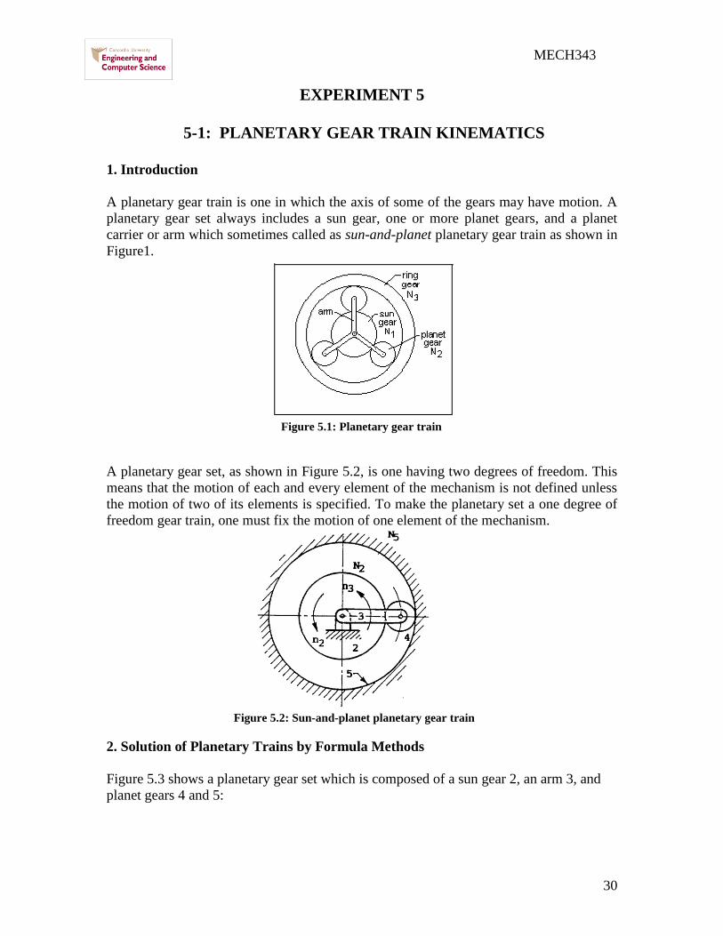
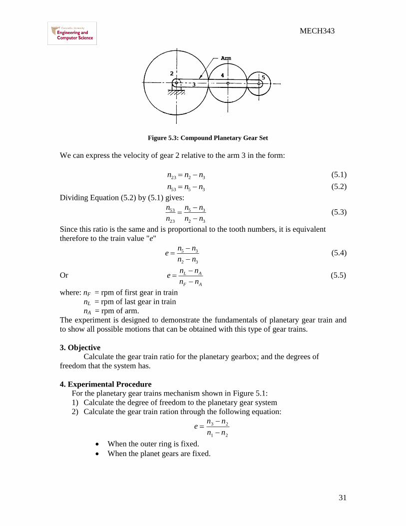
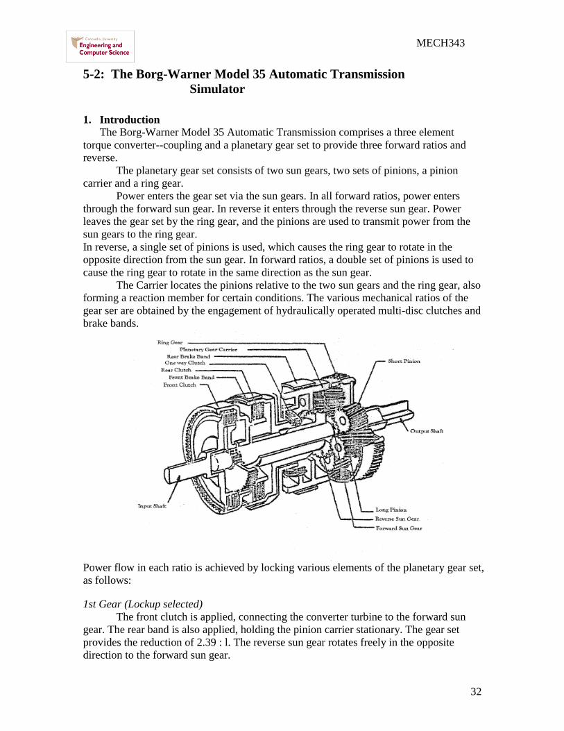
32
MECH343
5-2 The Borg-Warner Model 35 Automatic Transmission
Simulator
1 Introduction
The Borg-Warner Model 35 Automatic Transmission comprises a three element
torque converter--coupling and a planetary gear set to provide three forward ratios and
reverse
The planetary gear set consists of two sun gears two sets of pinions a pinion
carrier and a ring gear
Power enters the gear set via the sun gears In all forward ratios power enters
through the forward sun gear In reverse it enters through the reverse sun gear Power
leaves the gear set by the ring gear and the pinions are used to transmit power from the
sun gears to the ring gear
In reverse a single set of pinions is used which causes the ring gear to rotate in the
opposite direction from the sun gear In forward ratios a double set of pinions is used to
cause the ring gear to rotate in the same direction as the sun gear
The Carrier locates the pinions relative to the two sun gears and the ring gear also
forming a reaction member for certain conditions The various mechanical ratios of the
gear ser are obtained by the engagement of hydraulically operated multi-disc clutches and
brake bands
Power flow in each ratio is achieved by locking various elements of the planetary gear set
as follows
1st Gear (Lockup selected)
The front clutch is applied connecting the converter turbine to the forward sun
gear The rear band is also applied holding the pinion carrier stationary The gear set
provides the reduction of 239 l The reverse sun gear rotates freely in the opposite
direction to the forward sun gear
33
MECH343
1st Gear (Drive selected)
The front clutch is applied connecting the converter turbine to the forward sun
gear The one-way clutch is in operation preventing the pinion carrier from moving
opposite to the engine rotation The gear set again provides the reduction of 239 1 On
the overrun the one-way clutch unlocks and the gear set freewheels
2nd Gear (Lockup or drive selected)
Again the front clutch is applied connecting the converter turbine to the forward
sun gear The front band is applied holding the reverse sun gear stationary The pinions
now walk around the stationary sun gear and the gear set provides the reduction of 145
l
3rd Gear (Drive selected)
Again the front clutch is applied connecting the converter turbine to the forward
sun gear The rear clutch is applied connecting the turbine also to the reverse sun gear
Thus both sun gears are locked together and the gear set rotates as a unit providing a
ratio of 1 1
Neutral and Park
The front and rear clutches are released and no power is transmitted from the
converter to the gear set
Reverse
The rear clutch is applied connecting the converter turbine to the reverse sun gear
The rear band is applied holding the pinion carrier stationary providing a reduction of
209 l
2 Gear Ratios
119866119890119886119903 119877119886119905119894119900 120579119900120579119894
=1
239
The carrier is held stationary to provide the
reaction member and the gears operate as a
Simple gear train
34
MECH343
The reverse sun gear is held to that the gears
now operate as an epicyclic gear train
For an epicyclic gear train shown as following
119866119890119886119903 119877119886119905119894119900 120579119900120579119894
=1
145
119894134 =
1205961 minus 1205964
1205963 minus 1205964= minus
11988521198851
11988531198852prime
119900119903 120596119871
32
67= 120596119869 minus 120596119871 120596119869 =
99
67120596119871
For our transmission show as above
119894119865119869119871 =
120596119865minus120596119871
120596119869minus120596119871= minus
119885119866
119885119865
119885119867
119885119866
119885119869
119885119867=
67
28 (1)
119894119865119870119871 =
120596119865minus120596119871
120596119870minus120596119871= minus
119885119866
119885119865
119885119867
119885119866
119885119870
119885119867= minus
32
28 (2)
Hence minus120596119871
120596119869minus120596119871= minus
67
68
28
32
From (2) 120596119865 minus 120596119871 =32
28 120596119871 120596119865 =
60
28120596119871
Therefore 119894119865119869 =120596119865
120596119869=
60
28
67
99= 145021645
So 120579119900
120579119894=
1
145
35
MECH343
119866119890119886119903 119877119886119905119894119900 120579119900120579119894
=1
1
Both sun gears are locked together and the
gears set rotates as a unit
119866119890119886119903 119877119886119905119894119900 120579119900120579119894
=1
209
With the reverse gear engaged power is
applied to the reverse sun gear The planet
carrier is held stationary so that the planet
gears rotate the ring gear in the opposite
direction to the reverse sun gear
36
MECH343
3 Experimental Procedure
Pins and slotted plates represent the multi-disc clutches and brake bands The various
gear ratios of the gear set may be obtained by inserting the appropriate pins as indicated
below
A B C D E F
Lockup 1Drive 1
Lockup 2Drive 2
Drive 3
Reverse
Neutral
Park Note
1 Lose all pin and turn input shaft and output shaft make sure input shaft disk and
output shaft disk indicate to 0 then lock pins for each case
2 Turn input shaft one turn (360 ) read output disk (degree)
3 Fill out following table
Input (degree) Output (degree)
Lockup 1Drive 1 360
Lockup 2Drive 2 360
Drive 3 360
Reverse 360
4 Results
According to power flow and gear ratio figures for each case referring to 2nd gear
ratio calculation derive and calculate gear ratios for 1st 3
rd and reverse shift Compare
them with your experimental results
37
MECH343
EXPERIMENT 6
Static and Dynamic Balancing
1 Objective
The objectives of this experiment are
Understanding the concept of static and dynamic balancing
Understanding unbalance torque
Justifying theoretical calculation for balancing with experiment
Balancing the shaft by the four given masses
2 Introduction
Unbalanced dynamic forces effects have profound influence on the working and
of rotating machinery like turbines compressors pumps motors etc These forces act
directly on the bearings supporting the rotor and thus increase the loads and accelerate the
fatigue failure These unbalanced forces induce further mechanical vibrations in the
machinery and connected parts thereby creating environmental noise problem through
radiation of sound Hence it is desirable to balance all such uncompensated masses and
thus reduce the effect of unbalance forces in a dynamics balancing machine
Balancing is the technique of correcting or eliminating unwanted inertia forces which
cause vibrations which at high speeds may reach a dangerous level An important
requirement of all rotating machinery parts is that the rotation axis coincides with one of
the principal axis of inertia of the body After a roll is manufactured it must be balanced
to satisfy this requirement especially for high speed machines The condition of
unbalance of a rotating body may be classified as static or dynamic unbalance
2 1 Static Unbalance
An idler roll is statically balanced if the roll doesnt rotate to a heavy side when free to
turn on its bearings Thus the rolls center of gravity is on the axis of rotation Static
unbalance (Figure 61) creates a centrifugal force when rotating which causes deflection
of the roll Idler rolls are sometimes static
balanced only when the roll operates at slow
speeds
The static unbalance usually happens because
of errors in the manufacturing tolerances of
the rotating parts Therefore static imbalance
is essentially a weighing process in which the
part is acted upon by either gravitational or
centrifugal force This type of unbalance
could be easily reduced or removed by static
balancing
Figure 61 Static (or force) Unbalance
38
MECH343
2 2 Dynamic Unbalance
An idler roll may be in perfect static balance and not be in a balanced state when rotating
at high speeds A dynamic unbalance is a ldquocouplerdquo or twisting force in two separate
planes 180 degrees opposite each other (Figure 62) Because these forces are in
separate planes they cause a rocking motion from end to end A roll that is unbalanced
will cause 1) machinery vibrations 2) web
flutter and 3) a decrease in bearing life due to
unnecessary forces
To dynamically balance a roll it must first be
statically balanced Then the roll must be
rotated to its operating speed and have the
dynamic unbalance eliminated by adding or
subtracting weight The determination of the
magnitude and angular position of the
unbalance is the task of the balancing
machine and its operator Balancing
machines are provided with elastically
supported bearings in which the idler roll may
spin Because of the unbalance the bearings
will oscillate laterally and the amplitude and
phase of the roll are indicated by electrical
pickups and a strobe light
Figure 63 shows a long rotor which is to be mounted in bearing A and B We might
suppose that two equal masses m1 and m2 are placed at opposite ends of the rotor and at
equal distances r1 and r2 from the axis of rotation Since masses are equal on opposite
sides of the rotational axis the rotor is statically balanced in all angular positions But if
the rotor is caused to rotate at an angular velocity ω radsec the centrifugal forces m1r1ω2
and m2r2ω2 act respectively at m1 and m2 on the rotor ends These centrifugal forces
produce the equal but opposite bearing reactions FA and FB and the entire system of
forces rotate with the rotor at the angular velocity ω Thus the rotor is to be statically
balanced and at the same time dynamically unbalanced
Figure 63 Dynamically Unbalanced Rotor
Figure 62 Dynamic (or couple) Unbalance
39
MECH343
3 Principle and Theory of Operation
Consider a body of mass M rotating with a uniform angular velocity about O with
eccentricity e as shown in Figure 64 The centrifugal force Fc acting on the axis of
rotation is Me2 This force is therefore very sensitive to speed and hence there is a need
to reduce this force either by operating at lower speeds or by decreasing the eccentricity
as shown in Figure 65
O
e
M
M e
2
Figure 64 Unbalanced Disc
Center of rotation
( new center of
gravity )
Rotating Disc Added mass m
Center of gravityOriginal center
of gravity
(a) (b)
Figure 65 Illustration of The Simplest Method of Static Balancing
In general it is desirable to make e as low as possible If the rotor thickness to diameter
ratio is less than 05 and speed are below 1000 rpm the rotor can be single plane
balanced - otherwise two-plane balancing is necessary In the single plane balancing
technique with a rotor of mass mi and radius ri from the axis of rotation and lying in the
same plane the condition for static balance is used
0~iirm (61)
where i = 1 2 which denotes the total number of masses and m denotes the mass The
vector ir~ represents the eccentricity e of the mass mi from the axis of rotation
When the bodies are rotating in several planes the condition for dynamic balance has to
be satisfied in addition to that for static balance This is given by
0~~ iii rzm (62)
where iz~ is the axial coordinate vector of the mass mi measured for a chosen datum In
the two-plane balancing technique instead of satisfying Equations (61) and (62)
40
MECH343
explicitly Equation (62) is used with two different datum planes for iz~ Mathematically
if the distance between these two plane is oz~ then
0~)~~( ioii rzzm (63)
It is therefore clear that Equations (62) and (63) imply the satisfaction of Equation
(61) Conceptually it means that if a system of bodies rotating in several planes is in
dynamic balance with respect to two different datum planes then the system is also in
static balance This is the principle of the two-plane balancing technique
4 Description of Experimental Apparatus
Figure 66 shows the Static and Dynamic Balancing Apparatus It consists of a perfectly
balanced shaft with four rectangular blocks clamped to it The shaft is mounted in ball
bearings and it is driven by a 12 volt electric motor through a belt and pulley drive The
shaft assembly is mounted on a metal plate resting on four resilient rubber supports
which allow the mount to vibrate when the shaft is not balanced
The rectangular blocks can be clamped to the shaft at desired out-of-balance moments by
means of discs having eccentric holes of various diameters The discs are fixed to the
blocks by hexagon socket set screws Any longitudinal and angular position of a block
relative to the shaft can be set by linear and protractor scales provided Adjacent to the
linear scale is a slider which can be pushed against the block to read its longitudinal
position The slider also serves as a datum stop against which the blocks can be held
when reading their angular position on the shaft
The out-of-balance moments are measured by fitting the extension shaft and pulley to the
main shaft Each rectangular block is then clamped to the shaft in succession A cord with
a weight bucket at each end is hung on the pulley and bearing balls are placed in the
bucket until the block has turned through 90deg The out-of-balance moment is proportional
to the number of balls required
to turn the block
A Perspex dome serves as the
safety cover The shaft cannot
be driven unless the dome is in
position which is achieved by
micro switches actuated by the
dome The motor switch on the
front panel is spring loaded so
that the motor cannot be left
running The motor requires a
power supply of 12 volts at 2
amperes which is provided by
E66E90 speed controller
Figure 66 Static and Dynamic Balancing Apparatus
41
MECH343
5 Experimental Procedure
5 1 TEST 1 Static Balancing
1 Looking at the shaft from the side the masses will be as shown in figure 6-7
each mass has an angle θ with horizontal
Figure 6-7 Shaft view from the side
2 The masses forces are given by the following table 6-1
The masses values Table 6-1
3 In order to balance the shaft statically the sum of the forces will be equal zero
as the following equations
sum F=0
F1cos θ1+ F2cos θ2+ F3cos θ3+ F4cos θ4=0 (1)
F1sin θ1+ F2 sin θ2+ F3 sin θ3+ F4 sin θ4=0 (2)
4 Since we have just two equations with four unknown angles we assume
θ1=0ordm θ2=90ordm
5 Solving the two equations or using force polygon by AutoCAD to find the θ3
θ4
5 2 TEST 2 Dynamic balancing
1 Looking for the shaft from in front the masses create the forces as shown in
figure 6-8 each mass has an arm X create a momentum
F1
F2
F3
F4
42
MECH343
2 In order to balance the shaft dynamically the sum of the momentum will be
equal zero as the following equations
sum M=0
F1cos θ1X1+ F2cos θ2X2+ F3cos θ3X3+ F4cos θ4X4=0 (1)
F1sin θ1X1+ F2 sin θ2X2+ F3 sin θ3X3+ F4 sin θ4X4=0 (2)
3 Since we have just two equations with four unknown arms we assume
X1=50 mm X2=100 mm
4 Solving the two equations or using momentum polygon by AutoCAD to find
the X3 X 4
TABLE 6 2
Block 1 2 3 4
Mass 88 82 74 64
Angle θ(ordm) 0 90
Arm X (mm) 50 100
6 Typical Calculations
The basic equations that are used for balancing purposes are
0rW ii (63)
0rWa iii (64)
Suppose that block (1) is placed 17 mm from the left end of the shaft at zero angular displacement and that
block (2) is placed 100 mm from it at 120deg The measured out-of-balance moments are as follows
Figure 68 In front shaft view
43
MECH343
TABLE 6 3 OUT-OF-BALANCE MOMENTS
It is first necessary to draw the moment polygon of Wr values as shown in Figure 68 to determine the
angular positions of blocks (3) and (4) W1r1 and W2r2 are known in both magnitude and direction The
vector W1r1 has been drawn at positive X-direction (θ = 0) The lengths of vectors W3r3 and W4r4 are known
and arcs can be drawn from the ends of W1r1 and W2r2 to get the directions of the unknown vectors
Figure 69 shows the diagram of the angular positions and the corresponding longitudinal locations of the
blocks on the shaft are 17 mm for the first 117 mm for the second block
To find the longitudinal positions of the other two blocks we designate distance of block (3) by a3 and
distance of block (4) by a4 measured from block (1) so block (1) is the reference and will not appear in
calculations
Draw a vector a2W2r2 = 100 (82) units long parallel to r2 and vectors a3W3r3 and a4W4r4 parallel to r3 and r4
respectively so that the moment polygon is closed The lengths of vectors a3W3r3 and a4W4r4 can be
measured and the magnitudes found by using the scale factor From these a3 and a4 can be calculated
Notice that the sense of vector a3W3r3 is reverse In order to maintain vector a3W3r3 the only possible
solution is to reverse a3 So from the vector polygon (triangle) it follows
a3 = -12 mm
a4 = 124 mm
This means that block (3) should be located 5 mm from the left end of the shaft The blocks should be
positioned as follows
Block Angular Position (Deg) Longitudinal Position (mm)
(1) 0 17
(2) 120 117
(3) 190 5
(4) 294 141
The values of a3 and a4 can be found analytically using complex vector approach
Real and imaginary components yield
100(82) cos 120deg + (74) a3 cos 190deg + (64) a4 cos 294deg = 0
100(82) sin 120deg + (74) a3 sin 190deg + (64) a4 sin 294 deg = 0
which reduce to
4100- 7288 a3 -2603 a4 = 0
71014- 1285a3 -5847 a4 = 0
44
MECH343
Solving the two equations gives a3 = -1194mm a4 = 12396mm
The values compare very well with those obtained graphically
In order to obtain independent results it is suggested that Wr values of the blocks are varied by using
different positions of the discs with eccentric holes The angular displacements between blocks (1) and (2)
may also be varied
Figure 69 Moment Polygon of Wr
45
MECH343
EXPERIMENT 7
Machine Fault Simulator (MFS)
1 Theory
Refer to experiment number 6
2 Description of Experimental Apparatus
Figure 71 shows the machine fault simulator The rotor is driven by a variable speed
motor via a flat belt and the rotor rotational speed is captured through a digital
tachometer The vibration due to the unbalanced rotor is measured and fed directly into
the on-board processor of the machine
Figure 71 Machine Fault Simulator
3 Objective
In this experiment we will study the reaction of the shaft and the motor when the shaft is
balanced and when it is unbalanced
4 Experimental Procedure
1) Run the Vibro-Quest Software
o Define a ldquoNew Projectrdquo (under root)
o Fill up the window select ldquoProject namerdquo click ldquoNextrdquo
o Select ldquoNonerdquo from the menu on the right side click ldquoNextrdquo
Belt
Motor
Disk A Disk B
Reciprocating
Mechanism
Speed
Control
46
MECH343
o Review the table (do not change the default) click ldquoNextrdquo
o Review the table check the setting data click ldquoNextrdquo
o Click ldquoDonerdquo
o Review the information provided if they are not ok ldquoGo backrdquo to modify
the data then click ldquoFinishrdquo
2 Select ldquoDatardquo from the toll bar on the computer
3 Name the ldquoTest Titlerdquo in the window Insert the parameters used in the test and
click ldquoNextrdquo
4 Review the information provided in the window and click ldquoNextrdquo
5 Chose 2000 as Frequency limit 1600 for Space line Leave the rest information as
defaulted and ldquoGO DAQrdquo
2) Running the Machine Fault Simulator
Select the required speed (rpm) change it to frequency (Hz) using the following
relation 60)rpm(n2)Hz(f
1 Run the machine using speed control system at desired speed
2 Wait about 15 seconds to stable the system
3 Click onrdquo START RECORDINGrdquo
4 When the recording is finished save the file under the root of ldquoDatardquo of base line
at the subdirectory that you want to compare with the other data (for example if
you are running the machine at 20 Hz save the your file under 20 Hz subdirectory)
5 Now select the ldquoProject namerdquo from the left menu all the relevant tests will
appear at the right table under the ldquoTest Explorerrdquo
6 To compare the data from different files Hold down the ldquoShiftrdquo key and select
any two interested files that you are going to compare
7 Click on ldquoComparerdquo to observe the difference between the unbalanced system
with a base system
8 To observe more clearly the difference between the frequency responses of the
different test click on ldquoOverlayrdquo
TEST 1 Imbalance Effects on Vibration response
Install the defined weight in one of the taped hole in rotor disk A and tight it
securely with a nut
Close the cover of MFS
Change the motor speed and record vibration level at each bearing For this
purpose you don not need to define new project for each speed define a new
project( follow steps 1-6 from section 3) then follow steps 1-2 for each speed
from section 4
Measure the average level of amplitude at each speed and Plot it against the speed
Repeat steps 2-5 for 2 different weights at 2 different radius and angles
47
MECH343
TEST 2 Balancing the Imbalance Rotor
Add weight at different radius and angles using the ldquosample calculationrdquo to
balance the rotor
If the rotor is balanced define a ldquoNew projectrdquo and follow steps 3-8 of Section 4
Fill Table 7 1
TABLE 7 1
Unbalance weight on disc A ____________ angular position _______________
Mass Added on disk B gr r (mm)
Amp baseAmp New
48
MECH343
EXPERIMENT 8
DETERMINATION OF SPUR GEAR EFFICIENCY
1 Objective
The main objective of the experiment is to determine the efficiency of the
Spur gear and worm gear unit
2 Introduction and theoretical background
21 Pinion gear
Two intermeshed toothed wheels make up a pinion gear This type of gear
permits a positive transmission of motion and torque Wheel pairs are available in
different shapes and shaft configurations Figure 1 explains the various types of gears and
their arrangements
Fig8 1 Various types of gear arrangements
22 Worm gear
A worm gear is a screw-type transmission unit whose axes generally intersect at
right angles The worm and wheel make contact on a straight line Normally the worm
has a cylindrical core and the wheel globoid toothing Units with a very high performance
49
MECH343
consist of a globoid worm and globoid wheel A worm gear with a cylindrical worm has
the following special features
High load capacity compared with spur gears due to linear contact
Low-noise operation and high absorption of vibrations
Wide transmission range down to low ilt110
High efficiency at high transmission ratios high efficiencies(η le 98 ) can be
achieved with very sophisticated designs under favorable operating conditions a
decrease in pitch angle (high transmission ratio) or speed is accompanied by a
corresponding decrease in efficiency (to η le 50 )
Self-locking operation
Smaller and lighter design compared with spur bevel gear units possessing high
transmission ratios
23 Basic definitions
Drive torque
The drive torque is the product of the force F and the lever arm l on which the
force acts
M = F X l (1)
M is in Nm F is in N and l in m
Drive power
The drive power of a rotating shaft is the product of the torque M and angular
frequency ω P = M X ω (2)
and 60
2 n (3)
P is in W n is in rpm
Efficiency
The efficiency is defined as the ratio between the output and input powers It has a
maximum theoretical value of 1
in
out
P
P (4)
where speed i
nn 1
2
50
MECH343
3 Experimental set-up
Figure 2 shows the complete view of the experimental set up
Fig8 2 Complete view of GUNT AT 200 experimental set up
The modules comprising the drive unit spur gear worm gear and magnetic
powder brake are mounted on a profile frame The DC shunt motor is designed for right-
hand and left-hand rotation The drive unit is electrically powered via control housing
The control unit adjusts the DC machinersquos speed via its armature voltage Its target speed
is set by means of a potentiometer on this housing Its actual speed is measured and
indicated by means of an inductive proximity switch and evaluation unit The speed is
51
MECH343
measured inductively by a contactless sensor disc and indicated by a digital display
element on the control unit Electronic thyristor speed control with I x R compensation
provides a high torsional rigidity The reaction torque exerted on the drive housing is
measured by means of a spring force meter connected to a lever arm
The transmission units consist of a 2-stage spur gear with transmission
ratio i = 135 and a single-stage worm gear with transmission ratio i = 14The
transmission torque can be determined on the drive side as well as the brake side To
facilitate adjustment of the brake torque the brake characteristic (current torque) is
recorded in a preliminary experiment Moments are determined through power
measurements (spring balance) with a known lever arm The moments measured input
speeds and transmission ratios are used to determine power and efficiency
The magnetic powder coupling consists of two independently mounted
rotors ie a primary and a secondary rotor both furnished with ball bearings The
primary rotor also serves as a coil carrier If one of these two rotors is deactivated the
magnetic powder coupling can also be used as a brake The air gap between the two
rotors contains a special magnetic powder If a direct voltage is applied to the excitation
winding the powder aligns itself with the resulting magnetic field lines to form a
compact mass providing a frictional link between the primary and secondary rotors The
value of the torque depends on the adjusted current When the current-proportional
moment is exceeded slippage occurs without any transition
4 Experiments procedure
As shown in Figure 82 the complete view of the experimental set up for this
experiment there is input as the motor speed and the output as excitation current so that
there is two steps for this experiment
After making sure spur gear is connected as shown in Figure 83
1) Fix the output excitation current at I= 50 mA and change the speed of the motor as
shown in the table (1) each time measure the motor force F1 and the brake force F2
52
MECH343
Figure 83 Configuration of spur gear unit experimental set up
Measurement data to determine the efficiency of Spur gear unit Table (1) I = 50mA
SlNo Motor speed
( n1 ) rpm
Motor holding
force ( F1 ) N
Brake holding force
( F2 ) N
Efficiency ( η )
1 500
2 1000
3 1500
4 2000
5 2500
In order to find out the spur gear efficiency we go through the following equations
The general equation for the spur gear efficiency is
in
out
P
P
The drive power of a rotating shaft is the product of the torque M and angular
frequency ω P = M X ω
The drive torque is the product of the force F and the lever arm l on which the
force acts
M = F Arm
When the arm for the motor Arm1=25 mm and for the brake Arm2=50 mm
53
MECH343
And the angular velocity from the following equation
60
2 n
In order to find the speed for the brake we use this ratio assuming i= 135
i
nn 1
2
2) Fixing the input n1= 1500 rpm and changing the output and filling table (2)
Recorded values of the excitation current and the force on the lever arm table (2)
Speed n1= 1500 rpm
Excitation current I (mA) Force F2 on the lever arm (N)
50
70
90
110
130
150
130
110
90
70
50
5 Experiments Results
1) Plot the characteristics curve between the current I and the force on the lever arm
F2
2) Plot the characteristics curve between the current I and the torque M
3) Determine the efficiency of the spur gear unit Comment on the errors on the
efficiency if the calculated efficiency deviates from the realistic values of 80 -
90
54
MECH343
EXPERIMENT 9
ANALYSIS OF LINKAGE MECHANISM
Try to build a linkage mechanism as the figure below
Steps
1 Turn on grid line from View-workspace-grid lines as below
2 Select rectangle tool
55
MECH343
3 Click and drag a small rectangle
4 Click the rectangle copy it (CTRL+C) paste it (CTRL+V) two times
5 Change the length of each rectangle by selecting it and writing down the desired
length in the text box named W
Make the length as (3 ndash 332 - 4)
56
MECH343
6 Use the rotate tool and the select tool to arrange the rectangles
Make sure that the spacing is 4 units as shown below
7 Put a motor at the lower end of the left link
- First select the motor - Then click at the desired point
57
MECH343
8 Put a pin joint at the lower end of the right link
- First select the pin joint - Then click at the desired point
9 Put a point element at the remaining ends
- First double click (this
enable you to assign multiple
points) on the point element
It should look like below
58
MECH343
10 Join the links by selecting two points then selecting Join
Click the arrow select tool
Select first point ndash
press SHIFT and
click the other point
Press
Join
They should look like
below
11 Repeat the same for the remaining two points Your model should look like below
59
MECH343
12 Click RUN ( ) and watch it rotating
13 Now we want to capture the velocity of the joint between the left link and the middle
one
- Select it and click on Define ndash Vectors-
Velocity
Click Run and watch the velocity change
Note that by clicking on the link itself and defining the velocity the program calculates
the velocity of the CG of the link
14 Now you are ready to try different measurements
Acceleration Total Force Gravitational Force
60
MECH343
15 Select a link and use the measure tool
X- Position Graph
Y- Position Graph
61
MECH343
Measuring velocity values
16 Now try to change the length of any of the links and RUN the model and observe
for any change if any and explain
17 Change the mass of any of the links and observe for any change in velocity and
force And Why if there is any
18 Now double click on the motor (resetting the mass for any link that has been
changed) and notice that the value for velocity is 1 radsec Change this to make it the
same value for acceleration and torque Write what you observe and try to explain
19 Now increase the mass for one link (eg left one) gradual and see how this will
affect the motion for a fixed value for torque velocity or acceleration of the motor
20 Now replace the middle link with two links connected with total length as the
middle one run observe and explain
21 Based on (20) search for what is the equation relation or rule that governs the
mechanism motion
62
MECH343
EXPERIMENT 10
NUMERICAL DYNAMIC SIMULATION FLYWHEEL
Problem Definition
In the two cycle piston engine shown explosive gases are
ignited in the combustion chamber above the piston The
explosions apply a force of 150 N for the duration of every
downward stroke The engine is equipped with a speed
limiting device (rev limiter) which prevents the rotational
speed from exceeding a set value (red-line) The masses of
the piston and connecting rod are 075 kg and 15 kg
respectively The mass of the crankshaft-flywheel assembly
is 30 kg Given that the red-line of the engine is 35 radsec
(340 rpm) Assume the crankshaft-flywheel assembly can
be modeled as a circular disk
Objective
Determine the forces at the crankshaft bearing (point A) and connection rod (point B)
bearing
Solution
1 INTRODUCTION
Engines that exceed the manufacturers maximum speed (over-revving) may be subject to
excessive wear and possible failure To prevent over revving internal combustion
engines are often fitted with a device known as a rev-limiter When an engine exceeds its
red-line rev-limiters interrupt the ignition system slowing the engine down Once the
speed drops below the maximum the ignition system is switched back on In this exercise
you will model an internal combustion engine equipped with a rev-limiter The engine
has three bodies the piston the connecting rod and the crankshaft The piston will be
modeled by a square body The connecting rod will be modeled by a rectangular body
The crankshaft will be modeled as a circular body The bodies will be drawn sized and
joined to each other and the background The pistons cylinder walls will be modeled with
a keyed slot joint The force of combustion will be modeled by a force attached to the top
of the piston The resulting forces at the bearings will be measured
2 SETTING UP THE WORKSPACE
For this exercise three changes in the workspace will be made First for clarity the x-y
axes will be displayed The unit of distance will also be changed from meters (default) to
millimeters
63
MECH343
If the x-y axes are not currently displayed choose Workspace from the
View menu and choose XY Axes from the Workspace submenu The x-y
axes provide a reference frame for building a simulation
Choose Numbers and Unitshellip from the View menu The Numbers and
Units dialog appears
Click the More Choices button The dialog box expands
Click and hold in the Distance field (Figure 1) The pop-up menu appears
Choose millimeters from the Distance pop-up menu
Click in the Rotation field and choose Radians from the pop-up menu
Click OK
3 CREATING THE COMPONENTS
This exercise has three objects a 15 kg connecting rod a 075 kg piston and a 30 kg
crankshaft (see Figure 2 below) The connecting rod will be modeled by a thin rectangle
400 mm in length Its width will be thin 150 mm so it closely resembles the actual
connecting rod The crankshaft as stated in the exercise is modeled as a circular disk
with a 200 mm radius and a mass of 30 kg A 200 mm square object will represent the
piston The objects will be created sized and initialized in the following steps
Creating the Crankshaft
The crankshaft is represented by a circle with a radius of 200 mm and mass of 30 kg
These parameters will be set using the Geometry and Properties utility windows
I To draw the crankshaft
64
MECH343
bull Click the Circle tool in the Toolbar
bull Click once on the background Move the mouse to expand the circle and click
again to complete sketching
II To set the mass of the crankshaft
Choose Properties from the Window menu
Click the mass field and enter the value 30
III To set the size of the crankshaft
Select the crankshaft if it not already selected
Click the Radius field (labeled ldquorrdquo) of the Coordinates bar and enter the value 200
(Figure 3)
IV Zooming In
The circle will appear small after sizing To make the rectangle easier to manipulate and
appear larger the workspace will be magnified using the Zoom tool To zoom in
Click the Zoom In tool in the Toolbar
Click near the circle The objects in the window are magnified by a factor of two with
each click of the mouse To zoom out while the Zoom In tool is selected hold down
65
MECH343
the Shift key (the magnifying glass pointer changes to ldquo-rdquo) and click Your screen
should be similar to Figure 4 below
Figure 4 The workspace after zooming in
Click the Arrow tool in the Toolbar or press the spacebar to deselect the Zoom In
tool
Creating the Piston
For this exercise the piston will be modeled as a 200 mm square with the mass of 75 kg
The Square tool will be used to draw the piston and the Properties window will be used
to set its mass
I To draw the piston
Choose the Square tool in the Toolbar On systems the Square tool is ldquohiddenrdquo in the
RectangleSquare pop-up palette by default Click and hold on the Rectangle tool to
bring the pop-up palette in view (Figure 5 below)
Click once on the background drag to the right and click again to complete
sketching A square appears on the screen To set the size of the piston
Click in the Height or Width field of the Coordinates bar and enter 200 Either field
changes both the height and the width of the object so that it remains square
Figure 5 RectangleSquare pop-up palette
II To set the pistonrsquos mass
bull Select the piston if it not already selected
bull Choose Properties from the Window menu
66
MECH343
bull Click in the mass field and enter the value 075
Creating the Connecting Rod
In this exercise the connecting rod is represented by a rectangle drawn with the
Rectangle tool and sized using the Geometry window To approximate an actual
connecting rod the rectangle will be given a mass of 2 kg a height of 500 mm and a
width of 100 mm
To draw the connecting rod
I Choose the Rectangle tool in the Toolbar (On systems the Square tool used above
may have replaced the Rectangle tool in the Toolbar If so the Rectangle tool may be
selected from the hidden pop-up palette by clicking and holding on the Square tool in
the Toolbar)
II Click once on the background drag to the right and click again to complete
sketching A rectangle appears on the screen To set the mass of the connecting rod
bull Select the new rectangle if it not already selected
bull Choose Properties from the Window menu
bull Click in the Mass field and enter the value 2
To set the size of the rod
1 Click the Height field of the Coordinates bar and enter the value 500
2 Click the Width field of the Coordinates bar and enter the value 100 Your screen
should resemble Figure 6
Figure 6 The piston crankshaft and connecting rod
Creating the Points for Joining
The objects in this exercise are connected to each other and to the background (see Figure
7 below) The connections will be modeled by creating points and joining them These
points will be created with the Point tool and accurately positioned using the Properties
window
67
MECH343
Figure 7 The points which will be created and their coordinates
Creating Points on the Connecting Rod
Double-click the Point tool in the Toolbar Double-clicking selects a tool for
successive operations On systems the difference between single and double-clicking
is indicated in the Toolbar by shading a doubleclicked item is dark grey while a
single-clicked item is light grey
Place the mouse pointer over the connecting rod rectangle Find the snap point at the
top end of the connecting rod An X symbol appears at snap points Find the snap
point located at the midpoint of the top side of the connecting rod
To attach a point element click when the snap point located at the top end is visible
Observe that the point element is attached to the top end of the rod
In the same fashion attach another point element to the bottom end of the connecting
rod Your screen should resemble Figure 8
Figure 8 Connecting rod points in position
68
MECH343
Attaching Points to the Crankshaft
The crankshaft needs two points a center point representing the main bearing and an
outer point representing the connecting rod bearing These points will be accurately
positioned at the center and at 200 mm from the center of the circle To create and
position the crankshaft points
Make sure the Point tool is still selected Place the mouse pointer over the
crankshaft Find the snap point at the center of the circle
Click when the snap point at the center is visible A point element is attached to
the center of the circle
Place the mouse pointer near the left quadrant of the circle Find the snap point at
the left quadrant (Figure 9) As the mouse pointer nears the left quadrant of the
circle the snap point appears
Click when the snap point at the left quadrant is visible Another point element is
attached to the left quadrant of the circle
Figure 9 Snap point at the left quadrant of the circle
Attaching Points to the Piston
Two points need to be attached to the piston a square point and a point The square point
will be joined to the slot on the background to create a keyed slot joint The point will be
joined to another point on the connecting rod to form a pin joint The square point will be
positioned on the piston at the coordinates of (0 -50) The square point will be rotated 90deg
so that when joined to the slot the piston will not rotate This is because vertical slots are
defined as being rotated 90deg horizontal slots are defined as having 0deg rotation When a
square point is joined to a slot the rotations of the two objects are aligned
I The point will be positioned at (0 0) To create the points
Click the Square Point tool The cursor turns into a square point
Click anywhere on the piston Since the square point will be precisely position
using the Coordinates bar below it is not necessary to find a snap point
Click in the X field of the Coordinates bar and enter 0 If you attached the square
point on a snap point the x-field of the Coordinates bar may contain a formula
expression (such as body[3] width or (00)) Simply overwrite the entire
expression and enter 0
Press the tab key to move to the Y field of the Coordinates bar and enter -50
Again simply overwrite the y-field with the value -50
Choose the Properties in the Window menu The Properties window appears
In the angle field of the Properties window (marked by oslash) enter the value 1571
The value of 1571 radians is equivalent to 90deg The value will be displayed in a
69
MECH343
rounded form but internally the correct value will be used The pointrsquos y-position
is set to -50 so it will not interfere with the connecting rod joint
II To create the point
Click the Point tool
Place the pointer near the center of the square and find the snap point
Click when the snap point at the center is visible The point is created at the center
of the piston
Attaching a Point to the Background
A point representing the main bearing of the crankshaft must be placed on the
background The point can be placed anywhere on the background for clarity it will be
placed at the origin (0 0) To create and position the point
Click the Point tool
Place the mouse pointer near the origin Find the snap point that appears at the
origin Make sure that nobody is obstructing the origin The snap point does not
appear if the origin is covered by a body
Click when the snap point at the origin is visible Verify the position of the point
by noting the (x y) position in the Coordinates bar it should be (0 0) We now
name this point element so that it becomes easier to select later
Choose Appearance from the Window menu The Appearance window appears
In the name field (where it says Point) type Base Pin Since we will not be
needing the Appearance window for the rest of the exercise close the window by
(Windows) clicking the box marked ldquoXrdquo at the top-right corner of the window or
() clicking the box at the top-left corner of the window
Attaching a Slot to the Background
The cylinder walls of the engine will be modeled with a keyed slot joint The joint will be
made by joining the square point on the piston to a slot attached to the background The
slot can be located anywhere on the background as long as it is located on the
crankshaftrsquos centerline (the yaxis for this model)
To create and position the slot on the background
Choose the Vertical Slot tool in the Toolbar On systems the Vertical Slot tool
may be ldquohiddenrdquo in the Slot pop-up palette Click and hold on the Slot tool in the
Toolbar to bring the pop-up palette in view
Place the pointer near the point element attached to the origin Find the snap
point
Click when the snap point is visible A vertical slot appears
Creating Joints
In this exercise there are four joints (see Figure 10) The joints will connect the piston to
the slot the piston to the connecting rod the connecting rod to the crankshaft and the
crankshaft to the main bearing
70
MECH343
Figure 10 The points which will be joined
The following steps will demonstrate how to make these joints
I Joining the Piston to the Slot
In this example the piston slides in a cylinder The
cylinder will be modeled as a keyed slot joint The joint
is created by joining the square point on the piston to the
slot To create the keyed slot joint
Select the square point on the piston and while
holding down the Shift key select the slot The word
ldquoJoinrdquo of the Join button in the Toolbar changes
from gray to black indicating the two points can be
joined
Click the Join button in the Toolbar The piston
moves to the slot (see Figure 11) Joining the
Crankshaft to the Point on the Background The
crankshaft main bearing is modeled as a pin joint
The pin joint will be created by joining the point at
the center of the circle to the point at the origin
II To join the crankshaft to the origin
Choose Properties in the Window menu
From the selection pop-up menu located at the top of the
Properties window choose Base Pin (Figure 12) The
Base Pin is now selected
Hold the Shift key down and select the center point on
the crankshaft circle
Click the Join button The crankshaft circle moves to the
origin
To see how the circle representing the crankshaft is
constrained bring the mouse pointer over the circle hold
down the mouse button and drag the circle The circle
can rotate but is fixed to the Base Pin
Figure 11 Piston joined to the slot
Figure 12 Selecting an object in
the Properties window
71
MECH343
III Joining the Components
The piston connecting rod and crankshaft will now be joined together (see Figure
13) The following steps describe how to join them
Figure 13 Joining the components
IV To join the piston to the connecting rod
Select the (round) point on the piston and while holding
the Shift key down select the top point on the
connecting rod
Click the Join button The two objects will come
together
V To join the connecting rod to the crankshaft
Select the bottom point on the connecting rod and while
holding the Shift key down select the remaining (left)
point on the crankshaft
Click the Join button Your screen should resemble
Figure 14
Editing the collision property of a pair of bodies
The Smart Editor keeps joints together during editing To see this try dragging the
connecting rod The connecting rod will stay joined while it is dragged and the crankshaft
and piston will move accordingly When you are done dragging the rod move it back to
the approximate position shown in the problem description on the first page of this
exercise
Preventing a Collision
In Working Model objects which are directly connected to each other never collide
Notice that the piston and crankshaft may overlap when they are dragged during editing
Since the two objects are not directly connected they will collide when you run the
simulation To prevent the collision the Do Not Collide command will be used
To prevent a collision
Select the piston and while holding the Shift key down select the crankshaft
Figure 14 the completed engine
72
MECH343
Click and hold on the Object menu title in the menu bar (Figure 15) Notice that
there is a checkmark beside ldquoColliderdquo indicating that the pair of selected objects
will collide when you run the simulation
Choose Do Not Collide in the Object menu
Figure 15 Editing the collision property of a pair of bodies
Creating the Force
A 100 N force is applied at the top of the piston in the negative y-direction (down) The
force is only active while the piston is traveling with a negative y velocity The force will
be drawn using the Force tool and its magnitude and location will be set using the
Properties window
Drawing the Force
The force will be drawn in the downward direction using the
Force tool
To draw the force
Click the Force tool in the Toolbar
Place the pointer near the midpoint of the top end of
the piston Find the snap point
Click when the snap point is visible drag the mouse
upward and click again to create the force A force
attached to the piston appears (Figure 16) Do not be
concerned with the exact direction or magnitude of the
force for now
Sizing the Force
The forcersquos magnitude and direction will be set using the Coordinates bar To size the
force
bull Click the force vector to select the force
bull Click the Fy field of the Coordinates bar and type -100
bull Click the Fx field of the Coordinates bar and type 0 The force vector changes in
length to reflect its new magnitude
Figure 16 Creating a Force
73
MECH343
Timing the Force
The ignition timing of the engine must be simulated The problem states that the force is
active only on the downward stroke (ie when the piston has a negative velocity) The
rev-limiter cuts off combustion when the rotational velocity is greater than 35
radianssecond To simulate these conditions the ldquoand (ab)rdquo function will be
incorporated with the following formulas
To determine when the piston has a negative velocity use the following formula
body[c]vy lt 0
where c is the pistons object id number To determine the pistonrsquos id number place the
cursor over the piston and read the Status bar
To determine when the enginersquos speed is greater than 35 rads use the following
formula
body[d]vr lt 35
where d is the crankshafts object id number Use the Status bar as above to determine the
crankshaftrsquos id number
The complete equation is
and (body[c]vy lt 0 body[d]vr lt 35)
The complete equation will be placed in the Active When field in the forcersquos Properties
window Gravity will provide the initial downward velocity to start the engine
To set the timing of the force
Select the force
Choose Properties from the Window menu
Click in the Active When field at the bottom of the Properties window On
Windows systems you must first un-check the Always button before clicking in
the Active When field
Type the following formula (see Figure 17)and(body [c]vy lt0body[d]vrlt 35)
where c and d are the object id numbers of the piston and crankshaft respectively
The forcersquos rev-limiter equation is designed for counter-clockwise (positive)
engine rotation It is important that the
engine be ldquostartedrdquo in a position similar to
the figure on the first page of this section
If you want a rev-limiter which works in
both directions try incorporating the abs()
function into the formula
You can increase the width of the ldquoActive
whenrdquo field to view the entire equation by
resizing the Properties window
The simulation is ready to run
Click the Run button in the Toolbar The engine runs A warning may appear if
you run the engine long enough you can ignore the warning for now
When you are ready to continue click the Reset button in the Toolbar
Figure 17 Active When field is in
the property window for a Force
74
MECH343
Measuring Properties from the Simulation
A graph in conjunction with a digital meter is a nice way to illustrate the rotational speed
of the enginersquos crankshaft Two digital meters will be used to display the forces on the
bearings Follow the steps below to create these output devices
Displaying a Graph
The angular velocity of the crankshaft will be
displayed by a graph To create the graph
Select the crankshaft circle Four squares
ldquohandlesrdquo will appear around the circle
indicating that the circle is selected
Choose Velocity from the Measure menu
and Rotation Graph from the Velocity
submenu A meter resembling Figure 18
appears
Displaying Digital Force Meters
To display the digital force meters
bull Select the crankshaft-main bearing joint (see Figure 19)
bull Choose Force from the Measure menu A digital meter appears
bull Repeat for the connecting rod-crankshaft joint (see Figure 19)
A second digital meter appears You may need to move the meters
To move the meters
bull Select a meter
bull Drag it to any position you wish
Your window should resemble Figure 20
Running the Simulation
Run the simulation Notice that the angular velocity increases until it reaches 30 rads
This is so because we have turned off the force above 30 rads just as a rev limiter t urns
off the ignition of an engine above a certain speed
Figure 18 A Velocity Graph
Figure 19 The Force to be measured Figure 20 The completed workspace
75
MECH343
Modifying the Graph Display
You may notice that the axis labels occlude the numeric labels along the tick marks of the
plot You can modify the display options using the Appearance window For example to
turn off axis labels so that the numeric labels clearly appear
Select the velocity meter on the screen
Choose Appearance in the Window menuAlternatively you could press
Control+J (on Windows systems) or Command+J (on MacOS systems) to open
the window
Turn off the options titled ldquoLabelsrdquo and ldquoUnitsrdquo (Figure 21) You may wish to try
modifying other options and observe the effects on the graph meter
If you wish to show the meter coordinate axes click the check box labeled Axes
MODIFYING THE SIMULATION
Try modifying the masses of the crankshaft and connecting rod and notice how quickly
red-line is reached Also try changing the length of the connecting rod by repositioning
one of the joints
Figure 21 Appearance window for a meter
76
MECH343
Appendix
A Running the VibroQuest Software
1 Run the VibroQuest 2 New Project (under root)
3 Fill up the window click ldquoNextrdquo 4 Select ldquoNonerdquo click ldquoNextrdquo
1 2
3
4
5
6
77
MECH343
5 Review the table (do not change the default) click ldquoNextrdquo
6 Click ldquoNextrdquo
7 Click ldquoDonerdquo
8 Click (review the information provided if they are not ok go back to modify them)
ldquoFinishrdquo
B Run the machine according to the procedure
9 Select ldquoDatardquo from the toll bar on the computer
10 Name the ldquoTest Titlerdquo in the window Insert the parameters used in the test and click
ldquoNextrdquo
7
8
9
1
0
78
MECH343
11 Review the information provided in the window and click ldquoNextrdquo
12 Chose 2000 for Frequency limit 1600 for Space line Leave the rest information as
defaulted and ldquoGO DAQrdquo
13 ldquoSTART RECORDINGrdquo
14 When the recording is finished save the file under the root of Data of the file which
you are to compare with
15 Now select the project name from the left window all the relevant tests will appear at
the right window
16 Hold down the shift key and select two tests that you are going to compare
17 Click on Compare to observe the difference between the unbalanced systems with
base system
1
1 1
2
1
3
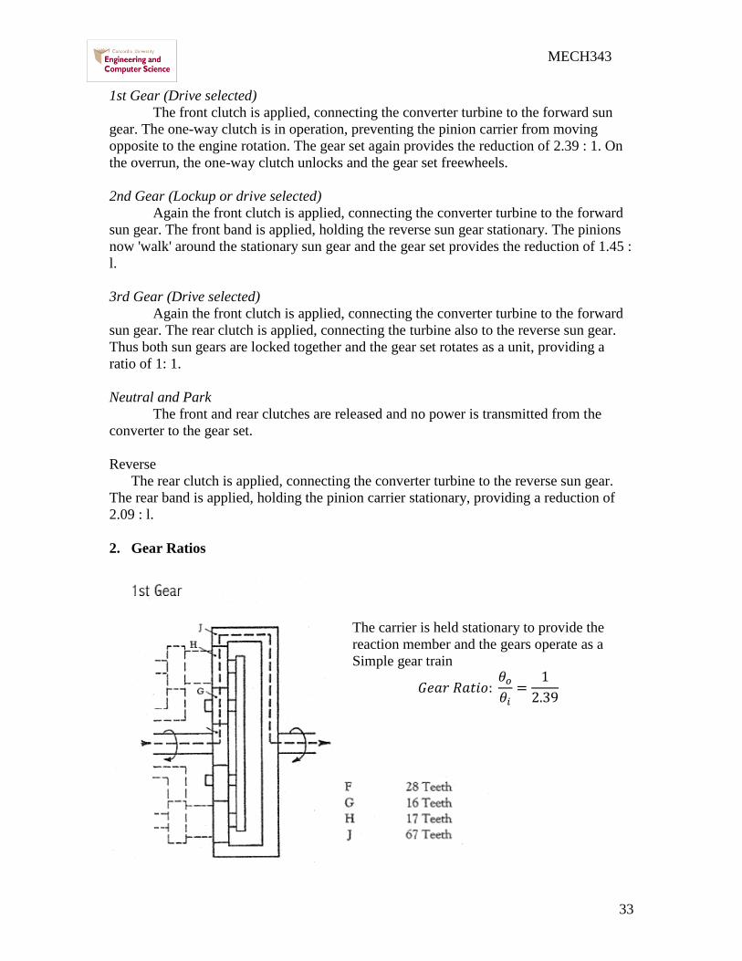
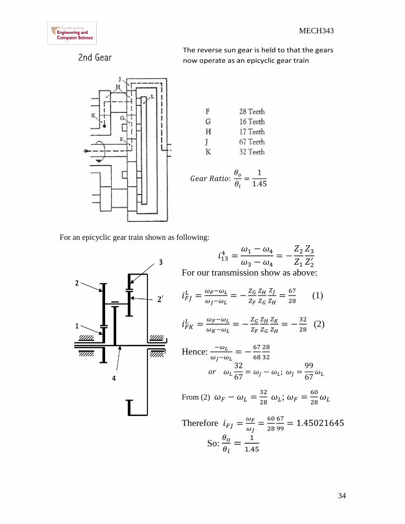
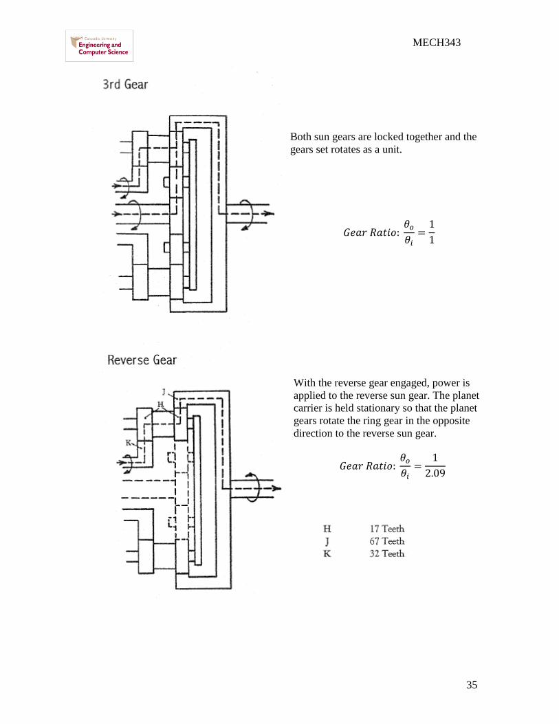
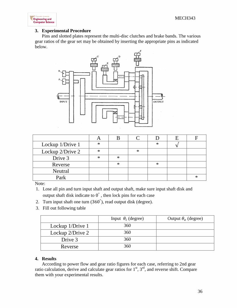
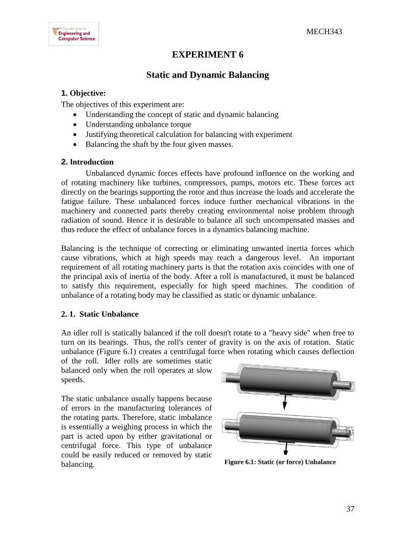
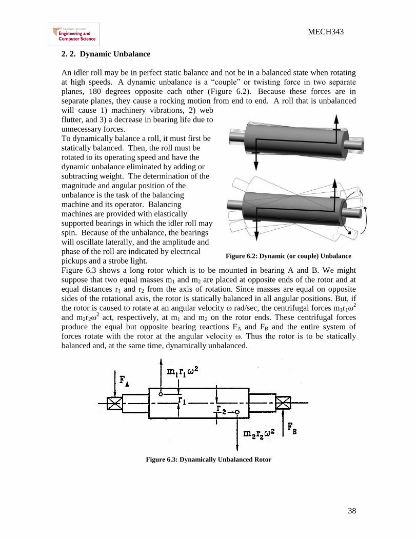
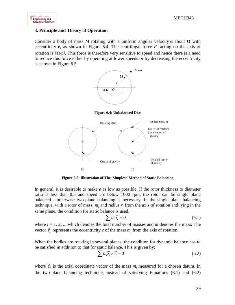
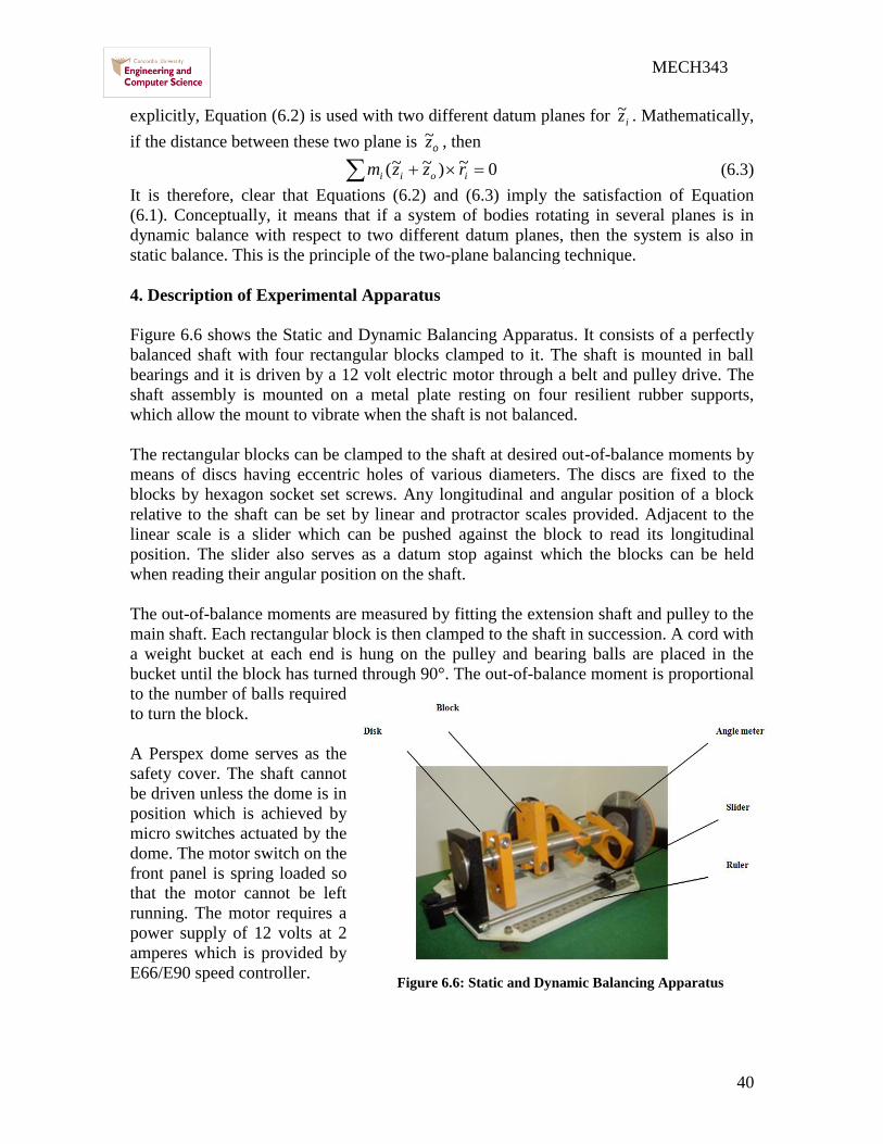
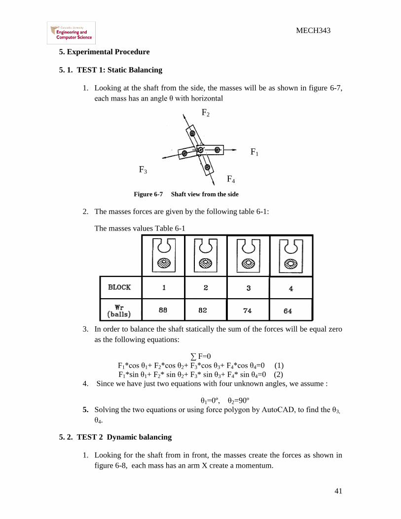
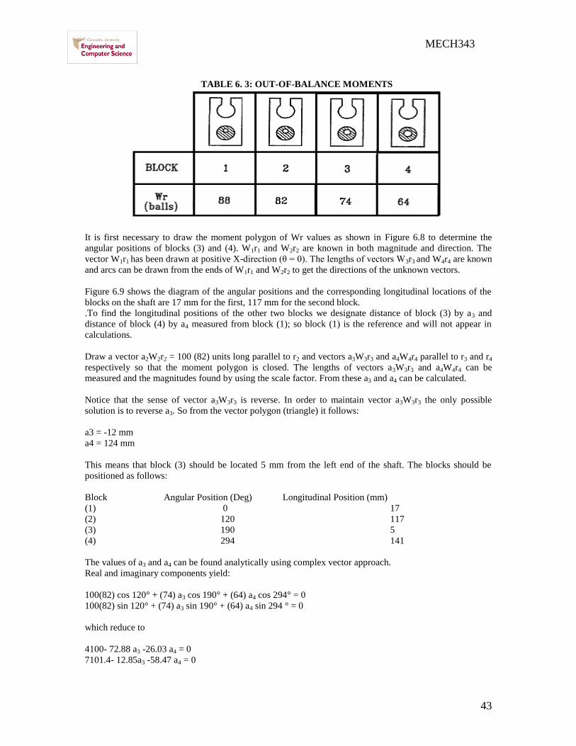
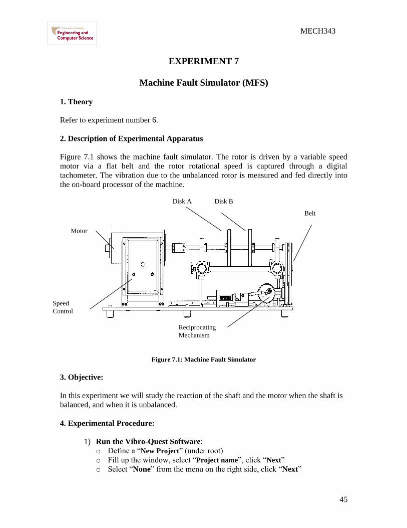
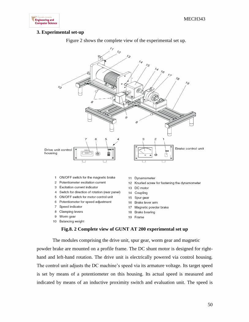
50
MECH343
3 Experimental set-up
Figure 2 shows the complete view of the experimental set up
Fig8 2 Complete view of GUNT AT 200 experimental set up
The modules comprising the drive unit spur gear worm gear and magnetic
powder brake are mounted on a profile frame The DC shunt motor is designed for right-
hand and left-hand rotation The drive unit is electrically powered via control housing
The control unit adjusts the DC machinersquos speed via its armature voltage Its target speed
is set by means of a potentiometer on this housing Its actual speed is measured and
indicated by means of an inductive proximity switch and evaluation unit The speed is
51
MECH343
measured inductively by a contactless sensor disc and indicated by a digital display
element on the control unit Electronic thyristor speed control with I x R compensation
provides a high torsional rigidity The reaction torque exerted on the drive housing is
measured by means of a spring force meter connected to a lever arm
The transmission units consist of a 2-stage spur gear with transmission
ratio i = 135 and a single-stage worm gear with transmission ratio i = 14The
transmission torque can be determined on the drive side as well as the brake side To
facilitate adjustment of the brake torque the brake characteristic (current torque) is
recorded in a preliminary experiment Moments are determined through power
measurements (spring balance) with a known lever arm The moments measured input
speeds and transmission ratios are used to determine power and efficiency
The magnetic powder coupling consists of two independently mounted
rotors ie a primary and a secondary rotor both furnished with ball bearings The
primary rotor also serves as a coil carrier If one of these two rotors is deactivated the
magnetic powder coupling can also be used as a brake The air gap between the two
rotors contains a special magnetic powder If a direct voltage is applied to the excitation
winding the powder aligns itself with the resulting magnetic field lines to form a
compact mass providing a frictional link between the primary and secondary rotors The
value of the torque depends on the adjusted current When the current-proportional
moment is exceeded slippage occurs without any transition
4 Experiments procedure
As shown in Figure 82 the complete view of the experimental set up for this
experiment there is input as the motor speed and the output as excitation current so that
there is two steps for this experiment
After making sure spur gear is connected as shown in Figure 83
1) Fix the output excitation current at I= 50 mA and change the speed of the motor as
shown in the table (1) each time measure the motor force F1 and the brake force F2
52
MECH343
Figure 83 Configuration of spur gear unit experimental set up
Measurement data to determine the efficiency of Spur gear unit Table (1) I = 50mA
SlNo Motor speed
( n1 ) rpm
Motor holding
force ( F1 ) N
Brake holding force
( F2 ) N
Efficiency ( η )
1 500
2 1000
3 1500
4 2000
5 2500
In order to find out the spur gear efficiency we go through the following equations
The general equation for the spur gear efficiency is
in
out
P
P
The drive power of a rotating shaft is the product of the torque M and angular
frequency ω P = M X ω
The drive torque is the product of the force F and the lever arm l on which the
force acts
M = F Arm
When the arm for the motor Arm1=25 mm and for the brake Arm2=50 mm
53
MECH343
And the angular velocity from the following equation
60
2 n
In order to find the speed for the brake we use this ratio assuming i= 135
i
nn 1
2
2) Fixing the input n1= 1500 rpm and changing the output and filling table (2)
Recorded values of the excitation current and the force on the lever arm table (2)
Speed n1= 1500 rpm
Excitation current I (mA) Force F2 on the lever arm (N)
50
70
90
110
130
150
130
110
90
70
50
5 Experiments Results
1) Plot the characteristics curve between the current I and the force on the lever arm
F2
2) Plot the characteristics curve between the current I and the torque M
3) Determine the efficiency of the spur gear unit Comment on the errors on the
efficiency if the calculated efficiency deviates from the realistic values of 80 -
90
54
MECH343
EXPERIMENT 9
ANALYSIS OF LINKAGE MECHANISM
Try to build a linkage mechanism as the figure below
Steps
1 Turn on grid line from View-workspace-grid lines as below
2 Select rectangle tool
55
MECH343
3 Click and drag a small rectangle
4 Click the rectangle copy it (CTRL+C) paste it (CTRL+V) two times
5 Change the length of each rectangle by selecting it and writing down the desired
length in the text box named W
Make the length as (3 ndash 332 - 4)
56
MECH343
6 Use the rotate tool and the select tool to arrange the rectangles
Make sure that the spacing is 4 units as shown below
7 Put a motor at the lower end of the left link
- First select the motor - Then click at the desired point
57
MECH343
8 Put a pin joint at the lower end of the right link
- First select the pin joint - Then click at the desired point
9 Put a point element at the remaining ends
- First double click (this
enable you to assign multiple
points) on the point element
It should look like below
58
MECH343
10 Join the links by selecting two points then selecting Join
Click the arrow select tool
Select first point ndash
press SHIFT and
click the other point
Press
Join
They should look like
below
11 Repeat the same for the remaining two points Your model should look like below
59
MECH343
12 Click RUN ( ) and watch it rotating
13 Now we want to capture the velocity of the joint between the left link and the middle
one
- Select it and click on Define ndash Vectors-
Velocity
Click Run and watch the velocity change
Note that by clicking on the link itself and defining the velocity the program calculates
the velocity of the CG of the link
14 Now you are ready to try different measurements
Acceleration Total Force Gravitational Force
60
MECH343
15 Select a link and use the measure tool
X- Position Graph
Y- Position Graph
61
MECH343
Measuring velocity values
16 Now try to change the length of any of the links and RUN the model and observe
for any change if any and explain
17 Change the mass of any of the links and observe for any change in velocity and
force And Why if there is any
18 Now double click on the motor (resetting the mass for any link that has been
changed) and notice that the value for velocity is 1 radsec Change this to make it the
same value for acceleration and torque Write what you observe and try to explain
19 Now increase the mass for one link (eg left one) gradual and see how this will
affect the motion for a fixed value for torque velocity or acceleration of the motor
20 Now replace the middle link with two links connected with total length as the
middle one run observe and explain
21 Based on (20) search for what is the equation relation or rule that governs the
mechanism motion
62
MECH343
EXPERIMENT 10
NUMERICAL DYNAMIC SIMULATION FLYWHEEL
Problem Definition
In the two cycle piston engine shown explosive gases are
ignited in the combustion chamber above the piston The
explosions apply a force of 150 N for the duration of every
downward stroke The engine is equipped with a speed
limiting device (rev limiter) which prevents the rotational
speed from exceeding a set value (red-line) The masses of
the piston and connecting rod are 075 kg and 15 kg
respectively The mass of the crankshaft-flywheel assembly
is 30 kg Given that the red-line of the engine is 35 radsec
(340 rpm) Assume the crankshaft-flywheel assembly can
be modeled as a circular disk
Objective
Determine the forces at the crankshaft bearing (point A) and connection rod (point B)
bearing
Solution
1 INTRODUCTION
Engines that exceed the manufacturers maximum speed (over-revving) may be subject to
excessive wear and possible failure To prevent over revving internal combustion
engines are often fitted with a device known as a rev-limiter When an engine exceeds its
red-line rev-limiters interrupt the ignition system slowing the engine down Once the
speed drops below the maximum the ignition system is switched back on In this exercise
you will model an internal combustion engine equipped with a rev-limiter The engine
has three bodies the piston the connecting rod and the crankshaft The piston will be
modeled by a square body The connecting rod will be modeled by a rectangular body
The crankshaft will be modeled as a circular body The bodies will be drawn sized and
joined to each other and the background The pistons cylinder walls will be modeled with
a keyed slot joint The force of combustion will be modeled by a force attached to the top
of the piston The resulting forces at the bearings will be measured
2 SETTING UP THE WORKSPACE
For this exercise three changes in the workspace will be made First for clarity the x-y
axes will be displayed The unit of distance will also be changed from meters (default) to
millimeters
63
MECH343
If the x-y axes are not currently displayed choose Workspace from the
View menu and choose XY Axes from the Workspace submenu The x-y
axes provide a reference frame for building a simulation
Choose Numbers and Unitshellip from the View menu The Numbers and
Units dialog appears
Click the More Choices button The dialog box expands
Click and hold in the Distance field (Figure 1) The pop-up menu appears
Choose millimeters from the Distance pop-up menu
Click in the Rotation field and choose Radians from the pop-up menu
Click OK
3 CREATING THE COMPONENTS
This exercise has three objects a 15 kg connecting rod a 075 kg piston and a 30 kg
crankshaft (see Figure 2 below) The connecting rod will be modeled by a thin rectangle
400 mm in length Its width will be thin 150 mm so it closely resembles the actual
connecting rod The crankshaft as stated in the exercise is modeled as a circular disk
with a 200 mm radius and a mass of 30 kg A 200 mm square object will represent the
piston The objects will be created sized and initialized in the following steps
Creating the Crankshaft
The crankshaft is represented by a circle with a radius of 200 mm and mass of 30 kg
These parameters will be set using the Geometry and Properties utility windows
I To draw the crankshaft
64
MECH343
bull Click the Circle tool in the Toolbar
bull Click once on the background Move the mouse to expand the circle and click
again to complete sketching
II To set the mass of the crankshaft
Choose Properties from the Window menu
Click the mass field and enter the value 30
III To set the size of the crankshaft
Select the crankshaft if it not already selected
Click the Radius field (labeled ldquorrdquo) of the Coordinates bar and enter the value 200
(Figure 3)
IV Zooming In
The circle will appear small after sizing To make the rectangle easier to manipulate and
appear larger the workspace will be magnified using the Zoom tool To zoom in
Click the Zoom In tool in the Toolbar
Click near the circle The objects in the window are magnified by a factor of two with
each click of the mouse To zoom out while the Zoom In tool is selected hold down
65
MECH343
the Shift key (the magnifying glass pointer changes to ldquo-rdquo) and click Your screen
should be similar to Figure 4 below
Figure 4 The workspace after zooming in
Click the Arrow tool in the Toolbar or press the spacebar to deselect the Zoom In
tool
Creating the Piston
For this exercise the piston will be modeled as a 200 mm square with the mass of 75 kg
The Square tool will be used to draw the piston and the Properties window will be used
to set its mass
I To draw the piston
Choose the Square tool in the Toolbar On systems the Square tool is ldquohiddenrdquo in the
RectangleSquare pop-up palette by default Click and hold on the Rectangle tool to
bring the pop-up palette in view (Figure 5 below)
Click once on the background drag to the right and click again to complete
sketching A square appears on the screen To set the size of the piston
Click in the Height or Width field of the Coordinates bar and enter 200 Either field
changes both the height and the width of the object so that it remains square
Figure 5 RectangleSquare pop-up palette
II To set the pistonrsquos mass
bull Select the piston if it not already selected
bull Choose Properties from the Window menu
66
MECH343
bull Click in the mass field and enter the value 075
Creating the Connecting Rod
In this exercise the connecting rod is represented by a rectangle drawn with the
Rectangle tool and sized using the Geometry window To approximate an actual
connecting rod the rectangle will be given a mass of 2 kg a height of 500 mm and a
width of 100 mm
To draw the connecting rod
I Choose the Rectangle tool in the Toolbar (On systems the Square tool used above
may have replaced the Rectangle tool in the Toolbar If so the Rectangle tool may be
selected from the hidden pop-up palette by clicking and holding on the Square tool in
the Toolbar)
II Click once on the background drag to the right and click again to complete
sketching A rectangle appears on the screen To set the mass of the connecting rod
bull Select the new rectangle if it not already selected
bull Choose Properties from the Window menu
bull Click in the Mass field and enter the value 2
To set the size of the rod
1 Click the Height field of the Coordinates bar and enter the value 500
2 Click the Width field of the Coordinates bar and enter the value 100 Your screen
should resemble Figure 6
Figure 6 The piston crankshaft and connecting rod
Creating the Points for Joining
The objects in this exercise are connected to each other and to the background (see Figure
7 below) The connections will be modeled by creating points and joining them These
points will be created with the Point tool and accurately positioned using the Properties
window
67
MECH343
Figure 7 The points which will be created and their coordinates
Creating Points on the Connecting Rod
Double-click the Point tool in the Toolbar Double-clicking selects a tool for
successive operations On systems the difference between single and double-clicking
is indicated in the Toolbar by shading a doubleclicked item is dark grey while a
single-clicked item is light grey
Place the mouse pointer over the connecting rod rectangle Find the snap point at the
top end of the connecting rod An X symbol appears at snap points Find the snap
point located at the midpoint of the top side of the connecting rod
To attach a point element click when the snap point located at the top end is visible
Observe that the point element is attached to the top end of the rod
In the same fashion attach another point element to the bottom end of the connecting
rod Your screen should resemble Figure 8
Figure 8 Connecting rod points in position
68
MECH343
Attaching Points to the Crankshaft
The crankshaft needs two points a center point representing the main bearing and an
outer point representing the connecting rod bearing These points will be accurately
positioned at the center and at 200 mm from the center of the circle To create and
position the crankshaft points
Make sure the Point tool is still selected Place the mouse pointer over the
crankshaft Find the snap point at the center of the circle
Click when the snap point at the center is visible A point element is attached to
the center of the circle
Place the mouse pointer near the left quadrant of the circle Find the snap point at
the left quadrant (Figure 9) As the mouse pointer nears the left quadrant of the
circle the snap point appears
Click when the snap point at the left quadrant is visible Another point element is
attached to the left quadrant of the circle
Figure 9 Snap point at the left quadrant of the circle
Attaching Points to the Piston
Two points need to be attached to the piston a square point and a point The square point
will be joined to the slot on the background to create a keyed slot joint The point will be
joined to another point on the connecting rod to form a pin joint The square point will be
positioned on the piston at the coordinates of (0 -50) The square point will be rotated 90deg
so that when joined to the slot the piston will not rotate This is because vertical slots are
defined as being rotated 90deg horizontal slots are defined as having 0deg rotation When a
square point is joined to a slot the rotations of the two objects are aligned
I The point will be positioned at (0 0) To create the points
Click the Square Point tool The cursor turns into a square point
Click anywhere on the piston Since the square point will be precisely position
using the Coordinates bar below it is not necessary to find a snap point
Click in the X field of the Coordinates bar and enter 0 If you attached the square
point on a snap point the x-field of the Coordinates bar may contain a formula
expression (such as body[3] width or (00)) Simply overwrite the entire
expression and enter 0
Press the tab key to move to the Y field of the Coordinates bar and enter -50
Again simply overwrite the y-field with the value -50
Choose the Properties in the Window menu The Properties window appears
In the angle field of the Properties window (marked by oslash) enter the value 1571
The value of 1571 radians is equivalent to 90deg The value will be displayed in a
69
MECH343
rounded form but internally the correct value will be used The pointrsquos y-position
is set to -50 so it will not interfere with the connecting rod joint
II To create the point
Click the Point tool
Place the pointer near the center of the square and find the snap point
Click when the snap point at the center is visible The point is created at the center
of the piston
Attaching a Point to the Background
A point representing the main bearing of the crankshaft must be placed on the
background The point can be placed anywhere on the background for clarity it will be
placed at the origin (0 0) To create and position the point
Click the Point tool
Place the mouse pointer near the origin Find the snap point that appears at the
origin Make sure that nobody is obstructing the origin The snap point does not
appear if the origin is covered by a body
Click when the snap point at the origin is visible Verify the position of the point
by noting the (x y) position in the Coordinates bar it should be (0 0) We now
name this point element so that it becomes easier to select later
Choose Appearance from the Window menu The Appearance window appears
In the name field (where it says Point) type Base Pin Since we will not be
needing the Appearance window for the rest of the exercise close the window by
(Windows) clicking the box marked ldquoXrdquo at the top-right corner of the window or
() clicking the box at the top-left corner of the window
Attaching a Slot to the Background
The cylinder walls of the engine will be modeled with a keyed slot joint The joint will be
made by joining the square point on the piston to a slot attached to the background The
slot can be located anywhere on the background as long as it is located on the
crankshaftrsquos centerline (the yaxis for this model)
To create and position the slot on the background
Choose the Vertical Slot tool in the Toolbar On systems the Vertical Slot tool
may be ldquohiddenrdquo in the Slot pop-up palette Click and hold on the Slot tool in the
Toolbar to bring the pop-up palette in view
Place the pointer near the point element attached to the origin Find the snap
point
Click when the snap point is visible A vertical slot appears
Creating Joints
In this exercise there are four joints (see Figure 10) The joints will connect the piston to
the slot the piston to the connecting rod the connecting rod to the crankshaft and the
crankshaft to the main bearing
70
MECH343
Figure 10 The points which will be joined
The following steps will demonstrate how to make these joints
I Joining the Piston to the Slot
In this example the piston slides in a cylinder The
cylinder will be modeled as a keyed slot joint The joint
is created by joining the square point on the piston to the
slot To create the keyed slot joint
Select the square point on the piston and while
holding down the Shift key select the slot The word
ldquoJoinrdquo of the Join button in the Toolbar changes
from gray to black indicating the two points can be
joined
Click the Join button in the Toolbar The piston
moves to the slot (see Figure 11) Joining the
Crankshaft to the Point on the Background The
crankshaft main bearing is modeled as a pin joint
The pin joint will be created by joining the point at
the center of the circle to the point at the origin
II To join the crankshaft to the origin
Choose Properties in the Window menu
From the selection pop-up menu located at the top of the
Properties window choose Base Pin (Figure 12) The
Base Pin is now selected
Hold the Shift key down and select the center point on
the crankshaft circle
Click the Join button The crankshaft circle moves to the
origin
To see how the circle representing the crankshaft is
constrained bring the mouse pointer over the circle hold
down the mouse button and drag the circle The circle
can rotate but is fixed to the Base Pin
Figure 11 Piston joined to the slot
Figure 12 Selecting an object in
the Properties window
71
MECH343
III Joining the Components
The piston connecting rod and crankshaft will now be joined together (see Figure
13) The following steps describe how to join them
Figure 13 Joining the components
IV To join the piston to the connecting rod
Select the (round) point on the piston and while holding
the Shift key down select the top point on the
connecting rod
Click the Join button The two objects will come
together
V To join the connecting rod to the crankshaft
Select the bottom point on the connecting rod and while
holding the Shift key down select the remaining (left)
point on the crankshaft
Click the Join button Your screen should resemble
Figure 14
Editing the collision property of a pair of bodies
The Smart Editor keeps joints together during editing To see this try dragging the
connecting rod The connecting rod will stay joined while it is dragged and the crankshaft
and piston will move accordingly When you are done dragging the rod move it back to
the approximate position shown in the problem description on the first page of this
exercise
Preventing a Collision
In Working Model objects which are directly connected to each other never collide
Notice that the piston and crankshaft may overlap when they are dragged during editing
Since the two objects are not directly connected they will collide when you run the
simulation To prevent the collision the Do Not Collide command will be used
To prevent a collision
Select the piston and while holding the Shift key down select the crankshaft
Figure 14 the completed engine
72
MECH343
Click and hold on the Object menu title in the menu bar (Figure 15) Notice that
there is a checkmark beside ldquoColliderdquo indicating that the pair of selected objects
will collide when you run the simulation
Choose Do Not Collide in the Object menu
Figure 15 Editing the collision property of a pair of bodies
Creating the Force
A 100 N force is applied at the top of the piston in the negative y-direction (down) The
force is only active while the piston is traveling with a negative y velocity The force will
be drawn using the Force tool and its magnitude and location will be set using the
Properties window
Drawing the Force
The force will be drawn in the downward direction using the
Force tool
To draw the force
Click the Force tool in the Toolbar
Place the pointer near the midpoint of the top end of
the piston Find the snap point
Click when the snap point is visible drag the mouse
upward and click again to create the force A force
attached to the piston appears (Figure 16) Do not be
concerned with the exact direction or magnitude of the
force for now
Sizing the Force
The forcersquos magnitude and direction will be set using the Coordinates bar To size the
force
bull Click the force vector to select the force
bull Click the Fy field of the Coordinates bar and type -100
bull Click the Fx field of the Coordinates bar and type 0 The force vector changes in
length to reflect its new magnitude
Figure 16 Creating a Force
73
MECH343
Timing the Force
The ignition timing of the engine must be simulated The problem states that the force is
active only on the downward stroke (ie when the piston has a negative velocity) The
rev-limiter cuts off combustion when the rotational velocity is greater than 35
radianssecond To simulate these conditions the ldquoand (ab)rdquo function will be
incorporated with the following formulas
To determine when the piston has a negative velocity use the following formula
body[c]vy lt 0
where c is the pistons object id number To determine the pistonrsquos id number place the
cursor over the piston and read the Status bar
To determine when the enginersquos speed is greater than 35 rads use the following
formula
body[d]vr lt 35
where d is the crankshafts object id number Use the Status bar as above to determine the
crankshaftrsquos id number
The complete equation is
and (body[c]vy lt 0 body[d]vr lt 35)
The complete equation will be placed in the Active When field in the forcersquos Properties
window Gravity will provide the initial downward velocity to start the engine
To set the timing of the force
Select the force
Choose Properties from the Window menu
Click in the Active When field at the bottom of the Properties window On
Windows systems you must first un-check the Always button before clicking in
the Active When field
Type the following formula (see Figure 17)and(body [c]vy lt0body[d]vrlt 35)
where c and d are the object id numbers of the piston and crankshaft respectively
The forcersquos rev-limiter equation is designed for counter-clockwise (positive)
engine rotation It is important that the
engine be ldquostartedrdquo in a position similar to
the figure on the first page of this section
If you want a rev-limiter which works in
both directions try incorporating the abs()
function into the formula
You can increase the width of the ldquoActive
whenrdquo field to view the entire equation by
resizing the Properties window
The simulation is ready to run
Click the Run button in the Toolbar The engine runs A warning may appear if
you run the engine long enough you can ignore the warning for now
When you are ready to continue click the Reset button in the Toolbar
Figure 17 Active When field is in
the property window for a Force
74
MECH343
Measuring Properties from the Simulation
A graph in conjunction with a digital meter is a nice way to illustrate the rotational speed
of the enginersquos crankshaft Two digital meters will be used to display the forces on the
bearings Follow the steps below to create these output devices
Displaying a Graph
The angular velocity of the crankshaft will be
displayed by a graph To create the graph
Select the crankshaft circle Four squares
ldquohandlesrdquo will appear around the circle
indicating that the circle is selected
Choose Velocity from the Measure menu
and Rotation Graph from the Velocity
submenu A meter resembling Figure 18
appears
Displaying Digital Force Meters
To display the digital force meters
bull Select the crankshaft-main bearing joint (see Figure 19)
bull Choose Force from the Measure menu A digital meter appears
bull Repeat for the connecting rod-crankshaft joint (see Figure 19)
A second digital meter appears You may need to move the meters
To move the meters
bull Select a meter
bull Drag it to any position you wish
Your window should resemble Figure 20
Running the Simulation
Run the simulation Notice that the angular velocity increases until it reaches 30 rads
This is so because we have turned off the force above 30 rads just as a rev limiter t urns
off the ignition of an engine above a certain speed
Figure 18 A Velocity Graph
Figure 19 The Force to be measured Figure 20 The completed workspace
75
MECH343
Modifying the Graph Display
You may notice that the axis labels occlude the numeric labels along the tick marks of the
plot You can modify the display options using the Appearance window For example to
turn off axis labels so that the numeric labels clearly appear
Select the velocity meter on the screen
Choose Appearance in the Window menuAlternatively you could press
Control+J (on Windows systems) or Command+J (on MacOS systems) to open
the window
Turn off the options titled ldquoLabelsrdquo and ldquoUnitsrdquo (Figure 21) You may wish to try
modifying other options and observe the effects on the graph meter
If you wish to show the meter coordinate axes click the check box labeled Axes
MODIFYING THE SIMULATION
Try modifying the masses of the crankshaft and connecting rod and notice how quickly
red-line is reached Also try changing the length of the connecting rod by repositioning
one of the joints
Figure 21 Appearance window for a meter
76
MECH343
Appendix
A Running the VibroQuest Software
1 Run the VibroQuest 2 New Project (under root)
3 Fill up the window click ldquoNextrdquo 4 Select ldquoNonerdquo click ldquoNextrdquo
1 2
3
4
5
6
77
MECH343
5 Review the table (do not change the default) click ldquoNextrdquo
6 Click ldquoNextrdquo
7 Click ldquoDonerdquo
8 Click (review the information provided if they are not ok go back to modify them)
ldquoFinishrdquo
B Run the machine according to the procedure
9 Select ldquoDatardquo from the toll bar on the computer
10 Name the ldquoTest Titlerdquo in the window Insert the parameters used in the test and click
ldquoNextrdquo
7
8
9
1
0
78
MECH343
11 Review the information provided in the window and click ldquoNextrdquo
12 Chose 2000 for Frequency limit 1600 for Space line Leave the rest information as
defaulted and ldquoGO DAQrdquo
13 ldquoSTART RECORDINGrdquo
14 When the recording is finished save the file under the root of Data of the file which
you are to compare with
15 Now select the project name from the left window all the relevant tests will appear at
the right window
16 Hold down the shift key and select two tests that you are going to compare
17 Click on Compare to observe the difference between the unbalanced systems with
base system
1
1 1
2
1
3
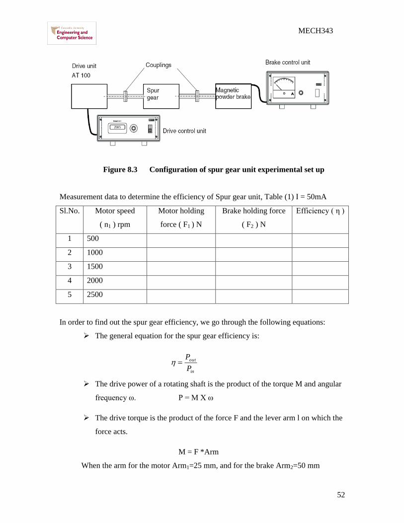
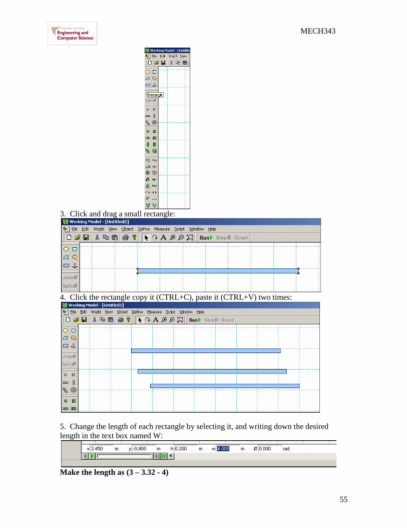
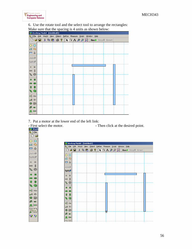
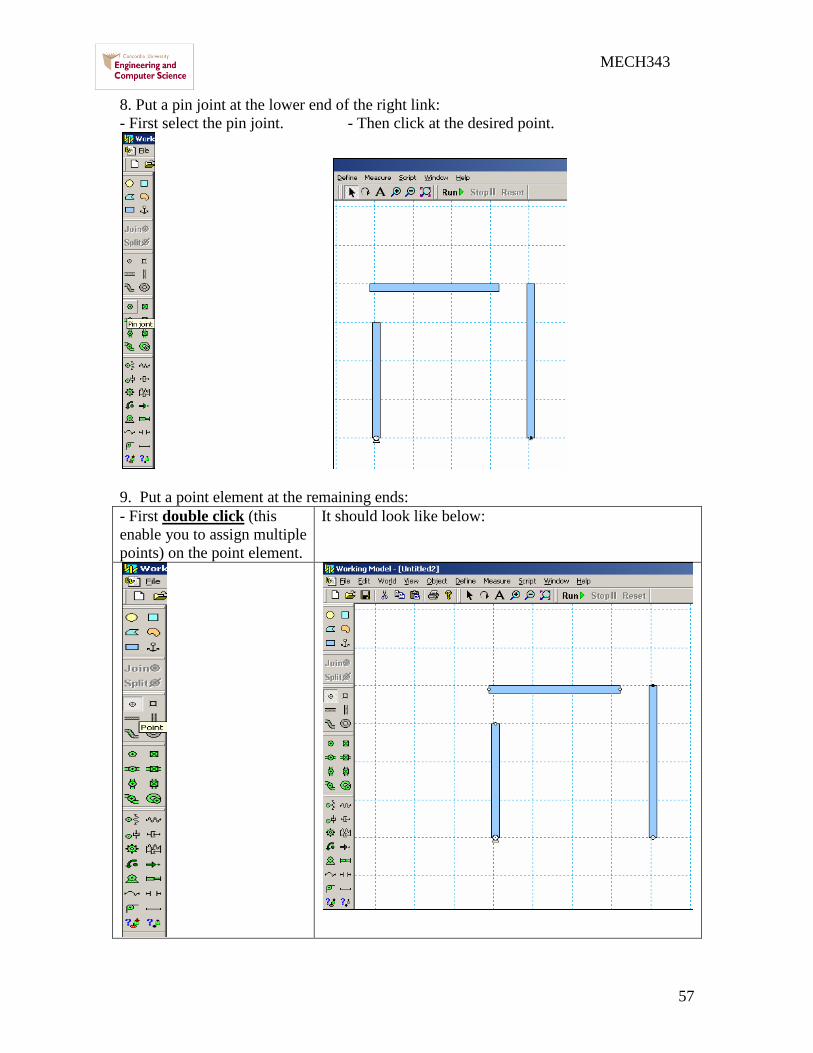
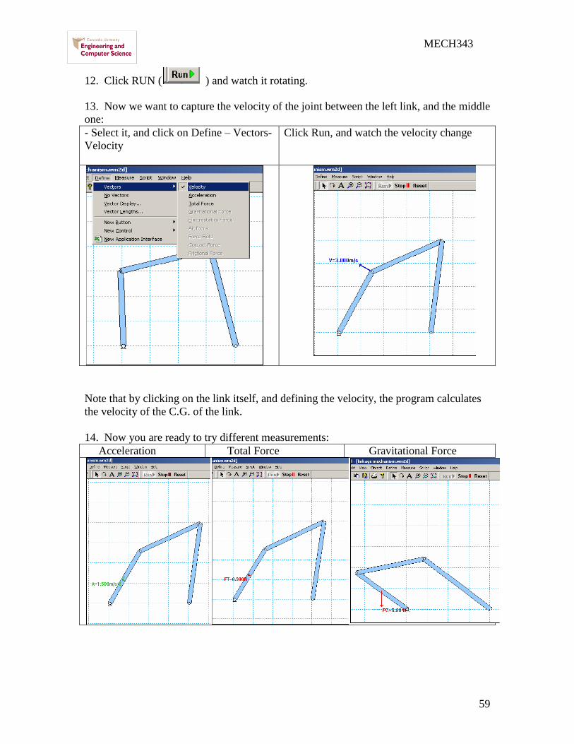
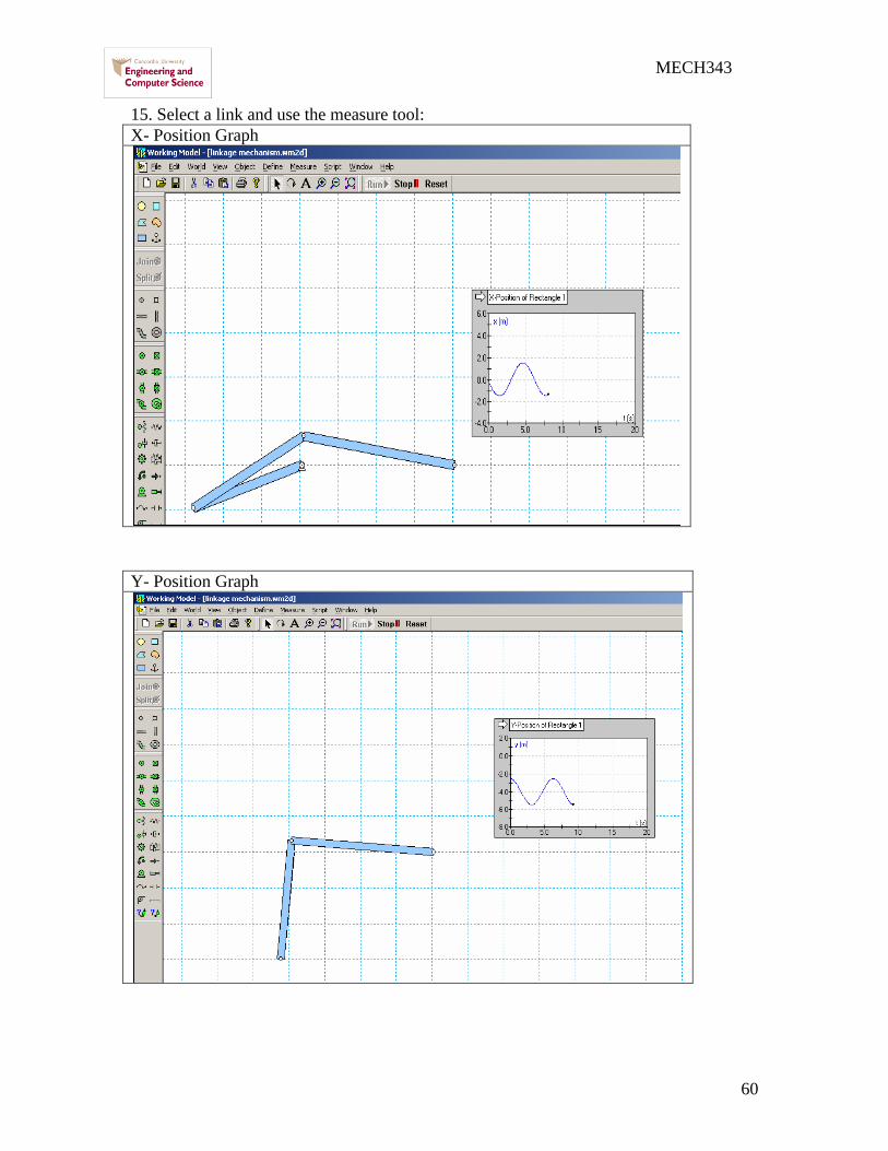
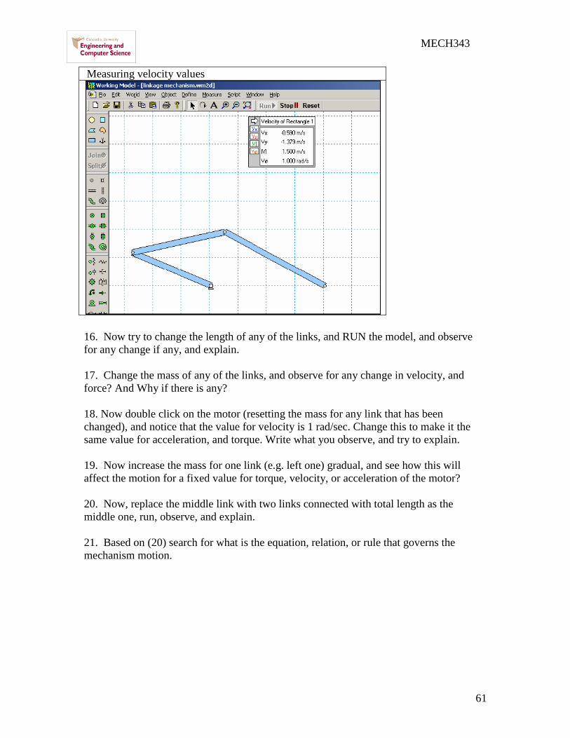
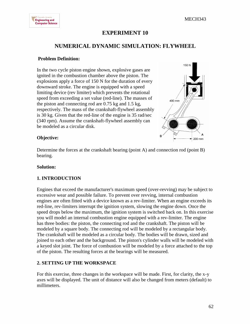
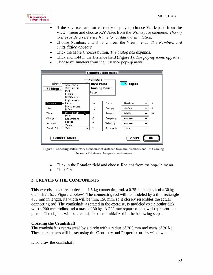
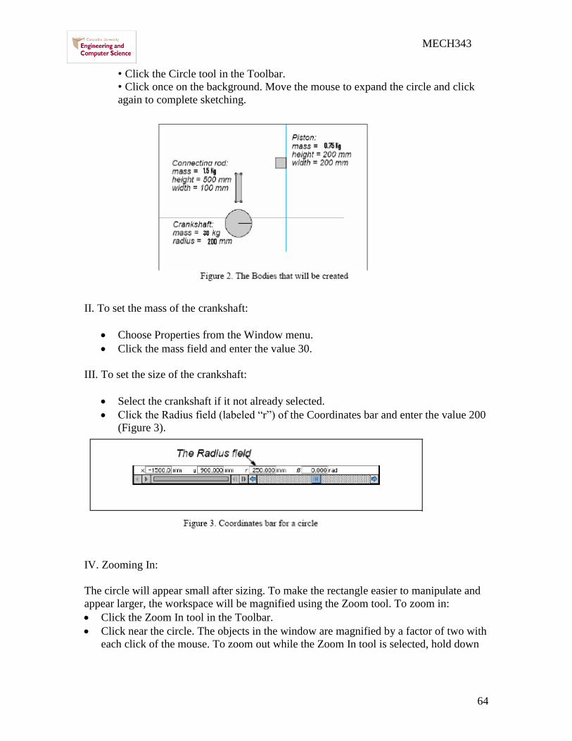
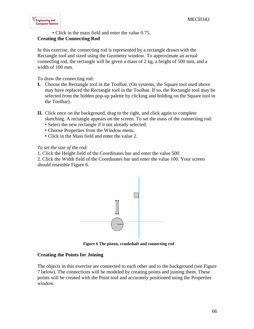
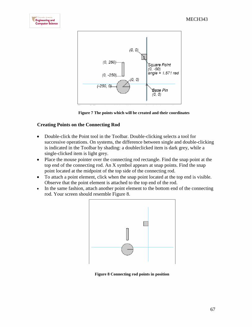
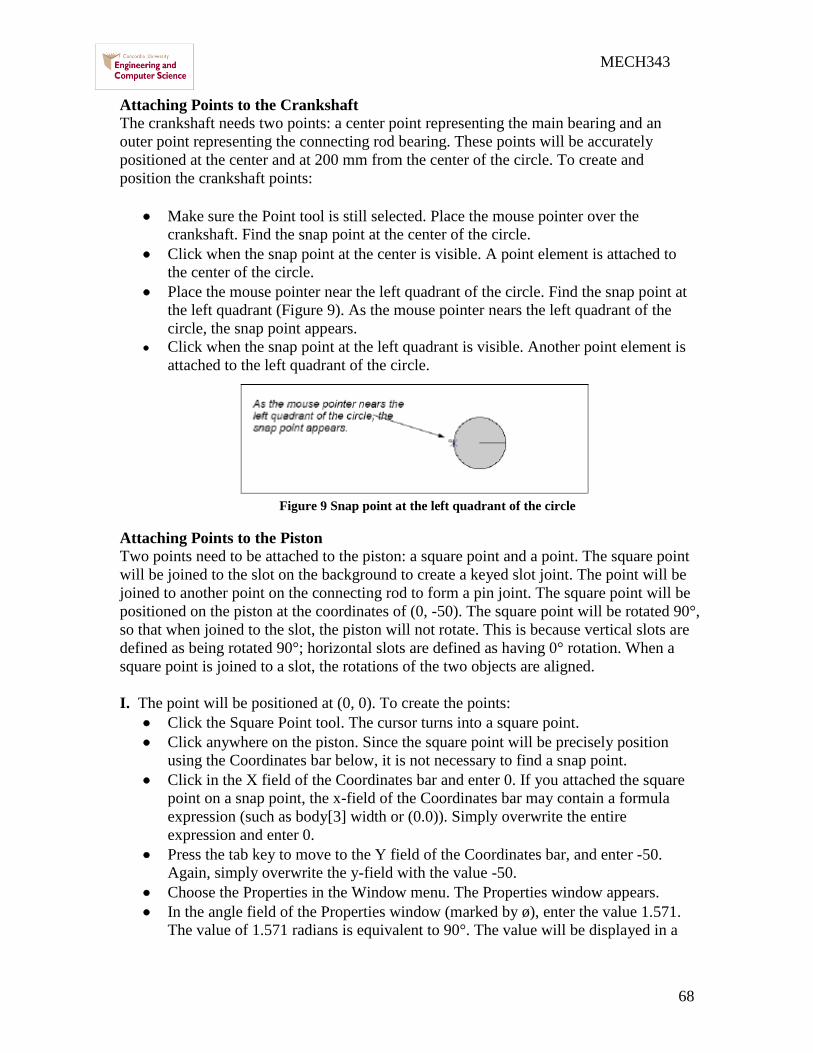
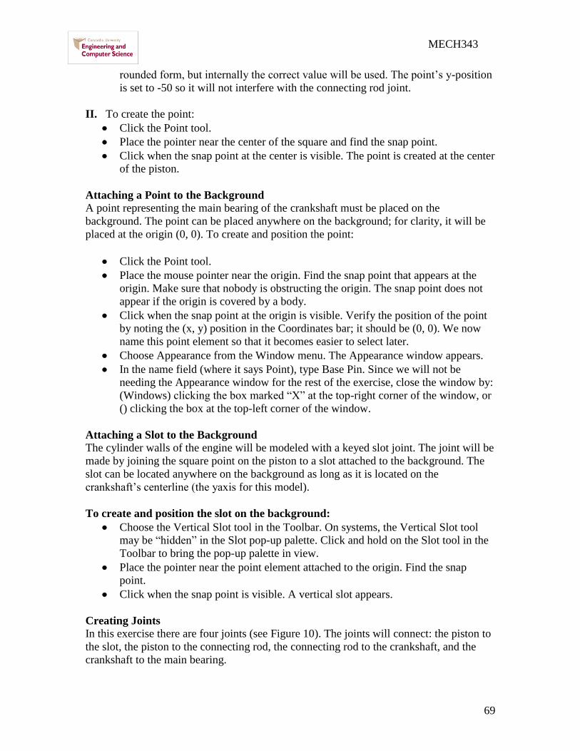
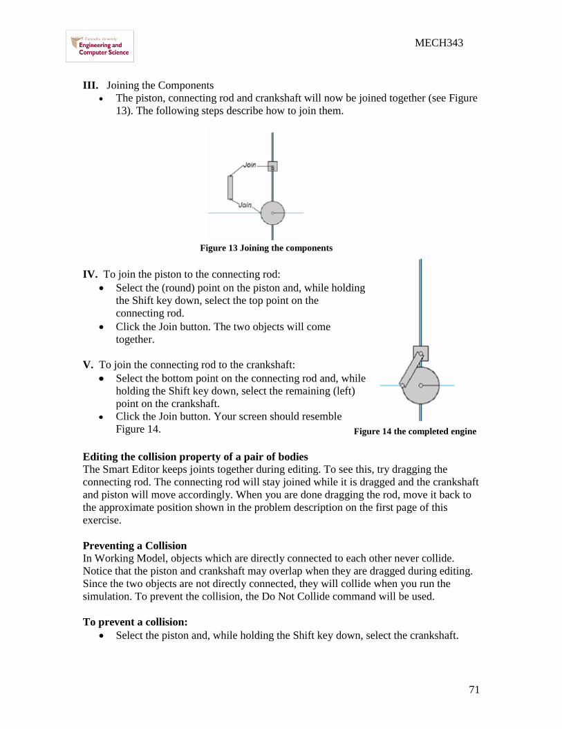
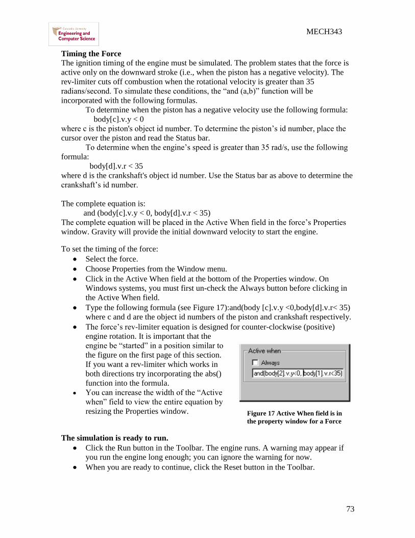
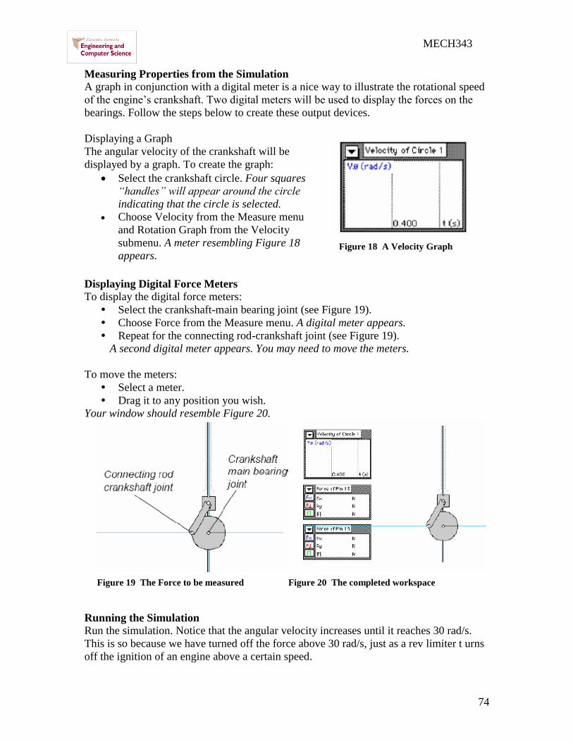
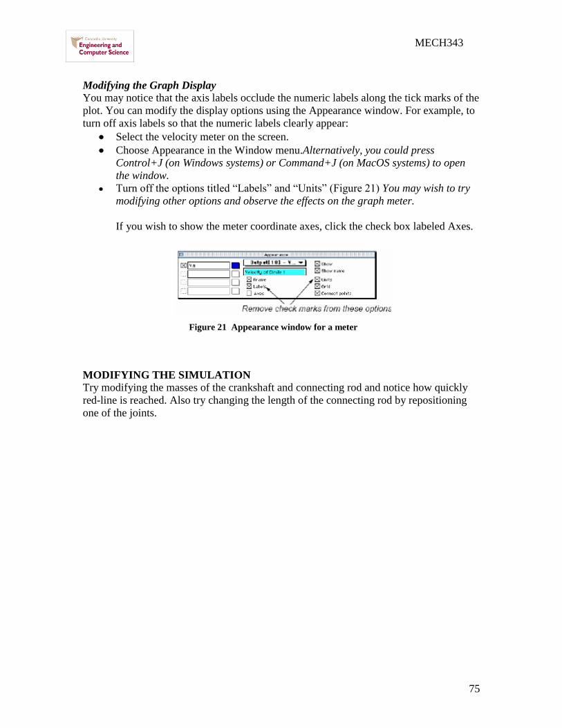
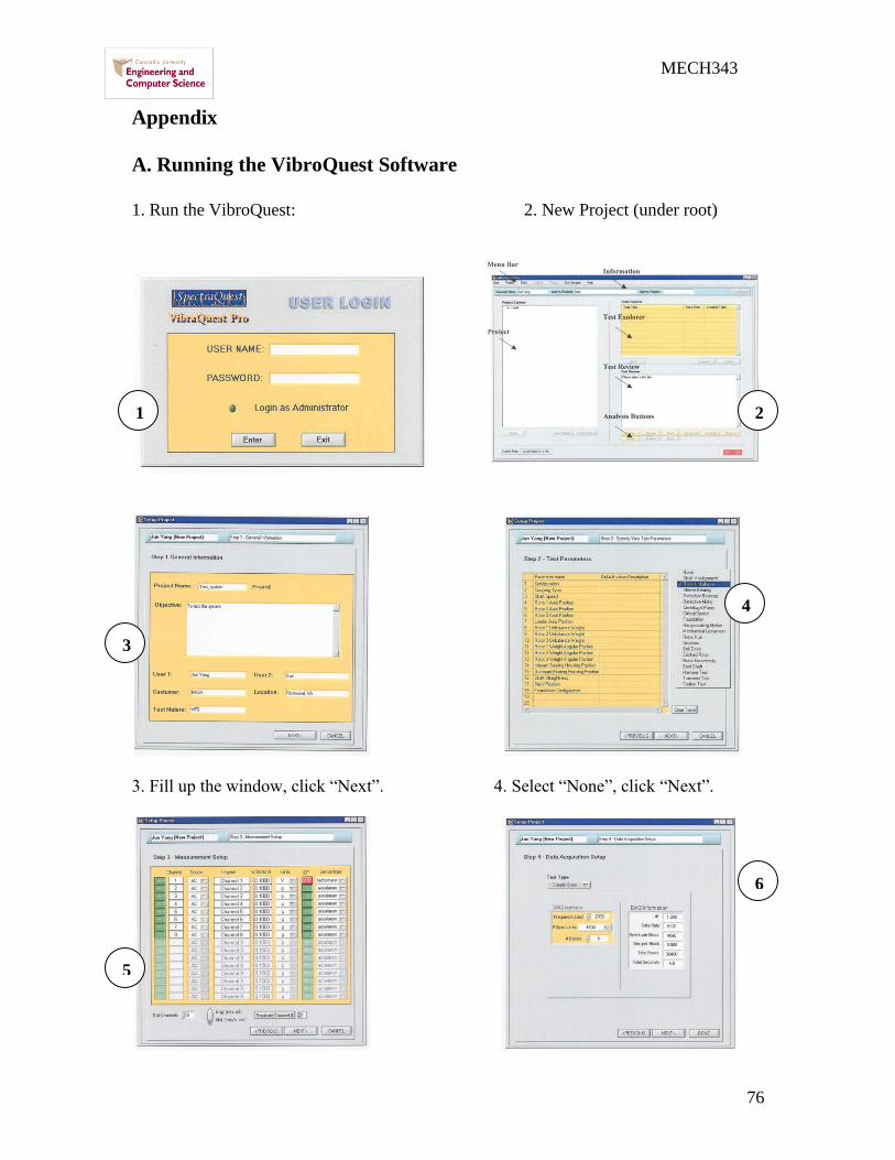
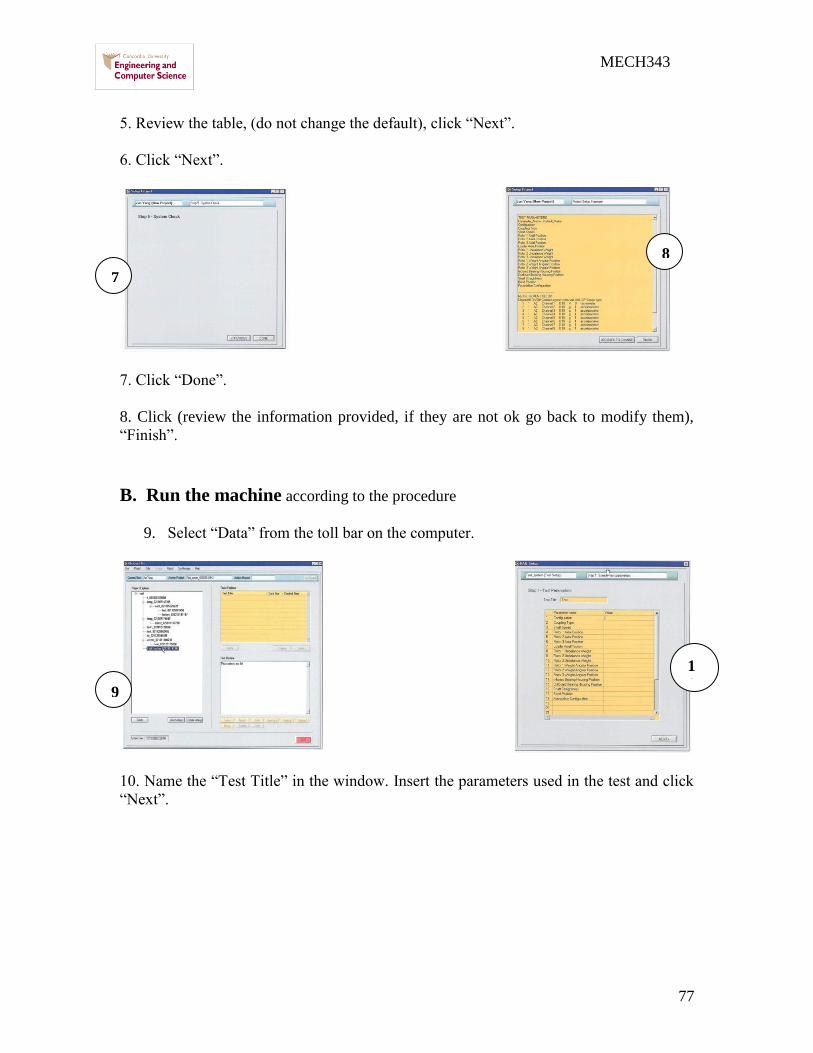
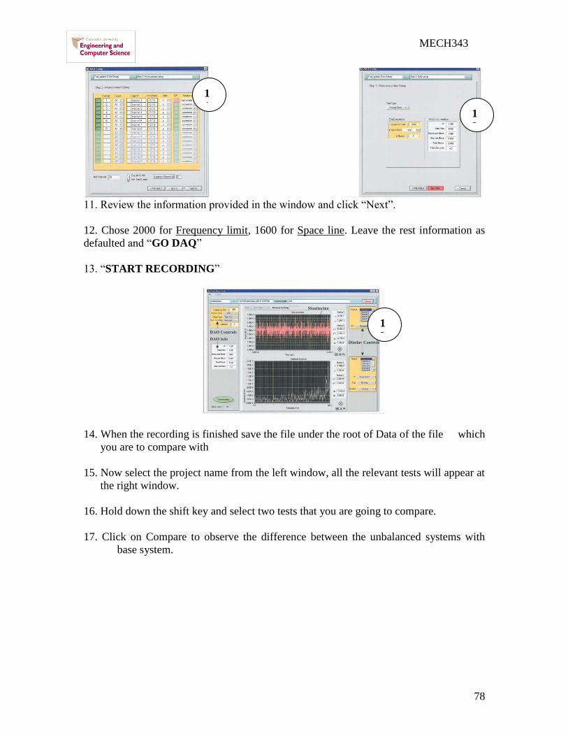