Laboratory 2: Amplitude Modulation

Cory J. Prust, Ph.D.Electrical Engineering and Computer Science DepartmentMilwaukee School of EngineeringLast Update: 17 December 2019

Contents

0 Laboratory Objectives and Student Outcomes 20.1 Laboratory Objectives . . . . . . . . . . . . . . . . . . . . . . . . . . . . . . . . . . . . . . . . 20.2 Student Outcomes . . . . . . . . . . . . . . . . . . . . . . . . . . . . . . . . . . . . . . . . . . 2

1 Background 3

2 Observing AM Waveforms 32.1 Frequency-domain . . . . . . . . . . . . . . . . . . . . . . . . . . . . . . . . . . . . . . . . . . 32.2 Time-domain . . . . . . . . . . . . . . . . . . . . . . . . . . . . . . . . . . . . . . . . . . . . . 4

3 Simulation of a QAM Transceiver 7

4 DSB-LC Receiver 94.1 DSB-LC Demodulation using the Complex Envelope . . . . . . . . . . . . . . . . . . . . . . . 94.2 Creating the Simulink model . . . . . . . . . . . . . . . . . . . . . . . . . . . . . . . . . . . . 10

5 Laboratory SDR Hardware and Installation 135.1 Ettus Research B200 USRP . . . . . . . . . . . . . . . . . . . . . . . . . . . . . . . . . . . . . 13

5.1.1 Installation in MATLAB/Simulink . . . . . . . . . . . . . . . . . . . . . . . . . . . . . 135.1.2 Verifying the Ettus B200 USRP Installation . . . . . . . . . . . . . . . . . . . . . . . . 14

6 DSB-LC Transmitter 156.1 Using MATLAB to generate the baseband DSB-LC signal . . . . . . . . . . . . . . . . . . . . 156.2 Creating the Simulink model . . . . . . . . . . . . . . . . . . . . . . . . . . . . . . . . . . . . 17

A Amplitude Modulation 19A.1 Double-Sideband Suppressed Carrier (DSB-SC) . . . . . . . . . . . . . . . . . . . . . . . . . . 19A.2 Double-Sideband Large Carrier (DSB-LC) . . . . . . . . . . . . . . . . . . . . . . . . . . . . . 20A.3 Quadrature Amplitude Modulation (QAM) . . . . . . . . . . . . . . . . . . . . . . . . . . . . 20

B Equivalence of Complex and I/Q Models 22

1

0 Laboratory Objectives and Student Outcomes

0.1 Laboratory Objectives

This laboratory will assist students in understanding the theoretical foundations of amplitude modulation.Students utilize SDR hardware to explore amplitude modulation. Additional topics include complex-envelopemodels, coherent and non-coherent detection, and quadrature-amplitude modulation.

0.2 Student Outcomes

Upon successful completion of this laboratory, the student will:

� Observe transmission of information using amplitude modulation over a wireless channel.

� Describe and characterize DSB-LC and DSB-SC waveforms based on time-domain and frequency-domain measurements.

� Explain the concept of frequency-division multiplexing.

� Utilize complex-envelope notation to describe amplitude modulated waveforms.

� Simulate transmission of two independent messages using quadrature-amplitude modulation.

� Construct a real-time DSB-LC receiver using their personal SDR device.

� Construct a real-time DSB-LC transmitter and broadcast a waveform that meets a radio-frequencychannel specification.

2

1 Background

Appendices A.1 and A.2 provide an overview and key results for double-sideband suppressed-carrier (DSB-SC) and double-sideband large-carrier (DSB-LC) communication systems, respectively.

Appendix A.3 provides an overview and key results for quadrature-amplitude modulated (QAM) communi-cation systems.

Appendix B describes the equivalence between the complex-valued signal models used in describing SDRtransceivers and I/Q transceivers.

2 Observing AM Waveforms

In this part of the laboratory you will use your personal SDR to observe amplitude modulated communicationsignals. Your instructor will broadcast radio-frequency signals in the laboratory at a frequency in the 902MHzto 928MHz frequency band.

The broadcast waveform consists of both a DSB-LC and a DSB-SC communication signal, separated fromone another by 30kHz. That is, the carrier frequencies of the two passband signals differ by 30kHz. Bothpassband signals are the result of modulating a sinusoidal carrier with a sinusoidal message signal.

2.1 Frequency-domain

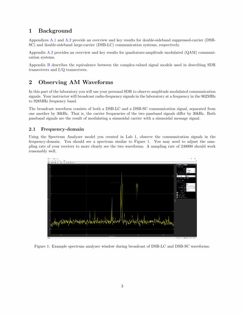
Using the Spectrum Analyzer model you created in Lab 1, observe the communication signals in thefrequency-domain. You should see a spectrum similar to Figure 1. You may need to adjust the sam-pling rate of your receiver to more clearly see the two waveforms. A sampling rate of 240000 should workreasonably well.

Figure 1: Example spectrum analyzer window during broadcast of DSB-LC and DSB-SC waveforms.

3

Question 2.1: Take a screen capture of the Spectrum Analyzer window. Annotate this imageby identifying the following:

� the DSB-LC communication signal

� the DSB-SC communication signal

� the upper and lower sidebands of the DSB-LC and DSB-SC signals

Question 2.2: What is the actual carrier frequency of the DSB-LC passband waveform that isbeing transmitted in the laboratory? What is the carrier frequency of the DSB-SC passbandwaveform? Explain how you arrived at your answers, referencing the Spectrum Analyzer screencaptures as necessary.

Question 2.3: What is the message frequency of the DSB-LC communication signal? Explainhow you arrived at your answer, referencing the Spectrum Analyzer screen captures as necessary.

Question 2.4: What is the message frequency of the DSB-SC communication signal? Explainhow you arrived at your answer, referencing the Spectrum Analyzer screen captures as necessary.

Question 2.5: Determine the modulation index of the DSB-LC communication signal usingmeasurements from its spectrum.

2.2 Time-domain

We will now add time-domain visualization to the Simulink model. The new model is shown in Figure 2.

Figure 2: Simulink model for viewing signals in the time-domain and frequency-domain.

� The Time Scope (found in DSP System Toolbox→ Sinks) block displays signals in the time domain,similar to an oscilloscope.

IMPORTANT: The Time Scope block defaults to a 10 second long display. When using highsampling rates (such as we often do), plotting 10 seconds of data can lead to sluggish (or even unstable)

4

behavior within Simulink. Before running a model that uses Time Scope blocks, adjust the time spanof each Time Scope block as follows:

– Double-click the Time Scope to open it

– Select View and Configuration Properties

– Select the Time tab and change the Time Span setting. You may want to initially choose One

frame period, and then refine the setting as you experiment with the model. You can specifyany duration you wish (e.g., set to 0.1 to show one tenth of a second).

� The Digital Filter Design (found in DSP System Toolbox→ Filtering→ Filter Implementations)block is used to isolate either the DSB-LC or DSB-SC waveforms by filtering the waveform at the out-put of the SDR receiver. Configure this block to implement a bandpass filter surrounding one, but notboth, of the AM signals. Without this isolation, the time domain plot would contain the superpositionof the two waveforms making it challenging to interpret. It is suggested to use a 40th order BandpassFIR Equiripple filter. You will need to set the stopband and passband frequencies according to yourspectrum observations. Consult with your instructor if you have questions.

IMPORTANT: Make sure the Input processing field (located in the lower left-hand corner of theparameter window) is set to Columns as channels (framed based).

� A second Spectrum Analyzer has been added to help in confirming operation of the bandpass filter.

You should see time domain waveforms similar to that shown Figure 3.

Figure 3: Example time scope window during broadcast of DSB-LC and DSB-SC waveforms.

5

Question 2.6: Take a screen capture of the Time Scope window showing the DSB-SC signal.Annotate this image by identifying the location/presence of the message signal. Determine themessage frequency.

Question 2.7: Take a screen capture of the Time Scope window showing the DSB-LC signal.Annotate this image by identifying the location/presence of the message signal. Determine themessage frequency.

Question 2.8: Determine the modulation index of the DSB-LC communication signal usingmeasurements from the time domain plot.

6

3 Simulation of a QAM Transceiver

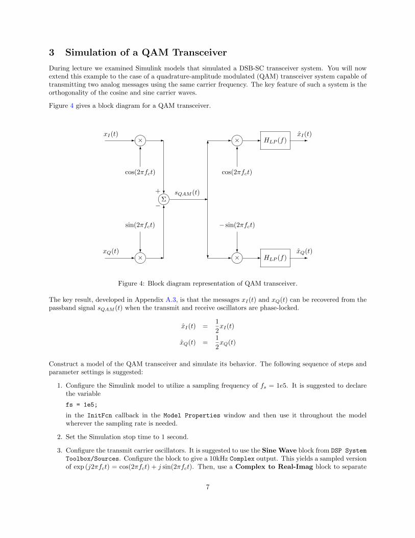
During lecture we examined Simulink models that simulated a DSB-SC transceiver system. You will nowextend this example to the case of a quadrature-amplitude modulated (QAM) transceiver system capable oftransmitting two analog messages using the same carrier frequency. The key feature of such a system is theorthogonality of the cosine and sine carrier waves.

Figure 4 gives a block diagram for a QAM transceiver.

-xI(t) � ��

×6

cos(2πfct)

-

?� ��Σ

+

−6

-sQAM (t)

-xQ(t) � ��

×?

sin(2πfct)

-

6-� ��×6

cos(2πfct)

- HLP (f) -xI(t)

? -� ��×?

− sin(2πfct)

- HLP (f) -xQ(t)

Figure 4: Block diagram representation of QAM transceiver.

The key result, developed in Appendix A.3, is that the messages xI(t) and xQ(t) can be recovered from thepassband signal sQAM (t) when the transmit and receive oscillators are phase-locked.

xI(t) =1

2xI(t)

xQ(t) =1

2xQ(t)

Construct a model of the QAM transceiver and simulate its behavior. The following sequence of steps andparameter settings is suggested:

1. Configure the Simulink model to utilize a sampling frequency of fs = 1e5. It is suggested to declarethe variable

fs = 1e5;

in the InitFcn callback in the Model Properties window and then use it throughout the modelwherever the sampling rate is needed.

2. Set the Simulation stop time to 1 second.

3. Configure the transmit carrier oscillators. It is suggested to use the Sine Wave block from DSP System

Toolbox/Sources. Configure the block to give a 10kHz Complex output. This yields a sampled versionof exp (j2πfct) = cos(2πfct) + j sin(2πfct). Then, use a Complex to Real-Imag block to separate

7

the cosine and sine carrier waveforms. Verify the carrier signals by connecting them to a Time Scopeblock and running the simulation.

4. Use additional Sine Wave blocks to create real-valued message signals for the in-phase and quadrature-phase message signals. Use a 800Hz sinusoid for the in-phase message. Use a 1500Hz sinusoid for thequadrature-phase message.

5. Add multiplier and adder blocks, bringing together the transmitter. Verify the transmitter by con-necting the output to Time Scope and Spectrum Analyzer blocks.

6. Construct the receiver. For our purposes, you may ignore the negative sign associated with thequadrature-phase oscillator (i.e., the sin term).

Initially, be sure the receiver carrier oscillators use the same Phase offset (rad) setting (a parameterof the Sine Wave block) as the transmit carriers. In this configuration, the receiver and transmitterwill be coherent.

Use the Digital Filter Design block from DSP System Toolbox/Filtering/Filter Designs. It issuggested to use a 40th order FIR filter, with passband edge frequency of 2000Hz.

IMPORTANT: Make sure the Input processing field (located in the lower left-hand corner of theparameter window) is set to Columns as channels (framed based).

7. Connect the transmitter output to the receiver and run the simulation, verifying that the in-phaseand quadrature outputs of the receiver match the original message waveforms. Use Time Scope andSpectrum Analyzer blocks as needed.

8. Simulate non-coherent behavior by adjusting the Phase offset (rad) setting of the receiver (or,equivalently, the transmitter).

Question 3.1: Submit a screen capture of your Simulink model. Appropriately label each ofthe key components, including naming Time Scope and Spectrum Analyzer blocks according tothe attached signals.

Question 3.2: For the case of coherent operation, submit screen captures of key simulationresults (time-domain and/or frequency domain waveforms) and explain the results. Yourresponse will be scored based on the accuracy and completeness of your explanations.

Question 3.3: For the case of non-coherent operation, submit screen captures of keysimulation results (time-domain and/or frequency domain waveforms) and explain the results.Your response will be scored based on the accuracy and completeness of your explanations.

8

4 DSB-LC Receiver

In this portion of the laboratory you will contruct a DSB-LC receiver using your personal SDR device. Youwill use this receiver to demodulate a voice signal that your instructor will broadcast in the laboratory. Thisform of AM voice communication has been used for many decades, and is still in use today. Air traffic controlcommunications, such as those between an airport control tower and approaching aircraft, utilize AM voicetransmissions in the VHF band.1

4.1 DSB-LC Demodulation using the Complex Envelope

Consider a DSB-LC passband signal of the form

sDSBLC(t) = [A+m(t)] cos(2πfct) (1)

where fc is the carrier frequency, m(t) is the message signal, and A is chosen such that A + m(t) > 0 forall values of t. This choice of A means that the information signal m(t) is contained in the envelope of thepassband signal.

Our demodulation strategy can be summarized as follows:

� Tune the receiver’s center frequency near, but not exactly to, the center frequency fc. In reality, itwould be extremely challenging to tune to exactly fc. Furthermore, even if we could, the oscillatorsin both the transmitter and receiver are likely to drift slightly over time (e.g., due to temperaturechanges). We will tune the receiver to fc − fi where fi << fc. The offset fi must be small enoughthat the DSB-LC signal remains within the instantaneous bandwidth of the SDR receiver.

� Filter the received signal to limit noise.

� Recover the message information by extracting the envelope of the received DSB-LC waveform. Thisis a form of non-coherent demodulation.

In reference to the complex signal model for an SDR receiver (see Appendix B), the SDR receiver generatessamples of z(t). Therefore, using the DSB-LC signal above we have

z(t) = LPF{sDSBLC(t)e−j(2π(fc−fi)t+φ)} (2)

where fi is the frequency offset and φ is a constant phase offset. Simplify this result:

z(t) = LPF{[A+m(t)] cos(2πfct)e−j(2π(fc−fi)t+φ)} (3)

= LPF{[A+m(t)]1

2(ej2πfct + e−j2πfct)e−j(2π(fc−fi)t+φ)} (4)

=1

2LPF{[A+m(t)](ej(2πfit−φ) + e−j(2π(2fc+fi)t−φ))} (5)

=1

2[A+m(t)]ej(2πfit−φ) (6)

where LPF{·} denotes the low pass filter operation that removes the double-frequency term near 2fc. Notethat fi is sufficiently small such that the signal of interest lies within the instantaneous bandwidth of thereceiver.

To recover the message signal, denoted m(t), we compute the magnitude of the complex signal z(t)

m(t) = |z(t)| (7)

=

∣∣∣∣12 [A+m(t)]ej(2πfit−φ)∣∣∣∣ (8)

1Students interested in learning more might start with https://en.wikipedia.org/wiki/Airband.

9

=1

2|A+m(t)|

∣∣∣ej(2πfit−φ)∣∣∣ (9)

=1

2[A+m(t)] (10)

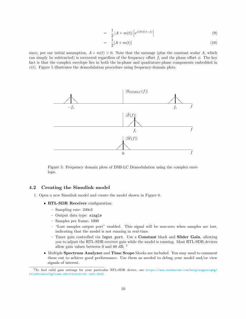
since, per our initial assumption, A + m(t) > 0. Note that the message (plus the constant scalar A, whichcan simply be subtracted) is recovered regardless of the frequency offset fi and the phase offset φ. The keyfact is that the complex envelope lies in both the in-phase and quadrature-phase components embedded inv(t). Figure 5 illustrates the demodulation procedure using frequency-domain plots.

|SDSBLC(f)|

f−fc fc

��@@

6��@@

6

|Z(f)|

ffi

��@@

6

|M(f)|

f0

��@@

6

Figure 5: Frequency domain plots of DSB-LC Demodulation using the complex enve-lope.

4.2 Creating the Simulink model

1. Open a new Simulink model and create the model shown in Figure 6.

� RTL-SDR Receiver configuration:

– Sampling rate: 240e3

– Output data type: single

– Samples per frame: 1000

– “Lost samples output port” enabled. This signal will be non-zero when samples are lost,indicating that the model is not running in real-time.

– Tuner gain controlled via Input port. Use a Constant block and Slider Gain, allowingyou to adjust the RTL-SDR receiver gain while the model is running. Most RTL-SDR devicesallow gain values between 0 and 60 dB. 2

� Multiple Spectrum Analyzer and Time Scope blocks are included. You may need to commentthese out to achieve good performance. Use them as needed to debug your model and/or viewsignals of interest.

2To find valid gain settings for your particular RTL-SDR device, see https://www.mathworks.com/help/supportpkg/

rtlsdrradio/ug/comm.sdrrtlreceiver.info.html

10

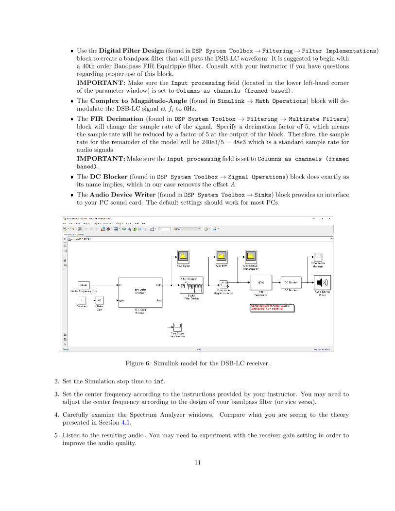
� Use the Digital Filter Design (found in DSP System Toolbox→ Filtering→ Filter Implementations)block to create a bandpass filter that will pass the DSB-LC waveform. It is suggested to begin witha 40th order Bandpass FIR Equiripple filter. Consult with your instructor if you have questionsregarding proper use of this block.

IMPORTANT: Make sure the Input processing field (located in the lower left-hand cornerof the parameter window) is set to Columns as channels (framed based).

� The Complex to Magnitude-Angle (found in Simulink → Math Operations) block will de-modulate the DSB-LC signal at fi to 0Hz.

� The FIR Decimation (found in DSP System Toolbox → Filtering → Multirate Filters)block will change the sample rate of the signal. Specify a decimation factor of 5, which meansthe sample rate will be reduced by a factor of 5 at the output of the block. Therefore, the samplerate for the remainder of the model will be 240e3/5 = 48e3 which is a standard sample rate foraudio signals.

IMPORTANT: Make sure the Input processing field is set to Columns as channels (framed

based).

� The DC Blocker (found in DSP System Toolbox → Signal Operations) block does exactly asits name implies, which in our case removes the offset A.

� The Audio Device Writer (found in DSP System Toolbox→ Sinks) block provides an interfaceto your PC sound card. The default settings should work for most PCs.

Figure 6: Simulink model for the DSB-LC receiver.

2. Set the Simulation stop time to inf.

3. Set the center frequency according to the instructions provided by your instructor. You may need toadjust the center frequency according to the design of your bandpass filter (or vice versa).

4. Carefully examine the Spectrum Analyzer windows. Compare what you are seeing to the theorypresented in Section 4.1.

5. Listen to the resulting audio. You may need to experiment with the receiver gain setting in order toimprove the audio quality.

11

Question 4.1: Submit screen captures of Spectrum Analyzer windows showing the varioussignals throughout the model. Provide brief explanations of what is seen in each capture.

Question 4.2: What happens to the recovered audio when you adjust the gain of the SDRreceiver block? Summarize your findings.

Question 4.3: What happens when you remove the Bandpass Filter from the model? Hint:You can do this easily by right-clicking the block and selecting “Comment Through”.Summarize your findings.

12

5 Laboratory SDR Hardware and Installation

5.1 Ettus Research B200 USRP

The Ettus Research [1] B200 Universal Software Radio Peripheral (USRP) is a high-performance software-radio transceiver providing high bandwidth, simultaneous transmit and receive operations, and numerousother advanced capabilities. The B200 communicates with a host PC through a USB 3.0 interface. It utilizesthe USRP Hardware Driver, or UHD [2], which is supported on Windows, Linux, and Mac OS X operatingsystems.

� Frequency Coverage: 70MHz to 6GHz

� Instantaneous Bandwidth: up to 56MHz

Figure 7: Ettus Research B200 USRP.

More detailed information on the B200 can be found in references [3] and [4]. MATLAB and Simulinkdocumentation is available at https://www.mathworks.com/hardware-support/usrp.html.

5.1.1 Installation in MATLAB/Simulink

Support for the B200 USRP is provided in MATLAB 2014b or later. To install:

1.

2. Navigate to the Home tab on the MATLAB Toolstrip, then to Add-Ons -> Get Hardware Support

Packages.

3. Search for “USRP” and choose the “Communications System Toolbox Support Package for USRPRadio” option.

4. Click the option to “Install”

5. You will need to log in to a Mathworks account in order to proceed. You can create one, if necessary.

6. You will be prompted to agree to various licensing agreements. Continue with the installation.

When the installation is complete, you should receive notification that “Your Hardware Support Packagerequires configuration.” If you have access to a USRP radio, choose “Setup Now” and continue with theinstallation. Otherwise you can resume configuration at a later time by typing targetupdater at theMATLAB command prompt.

13

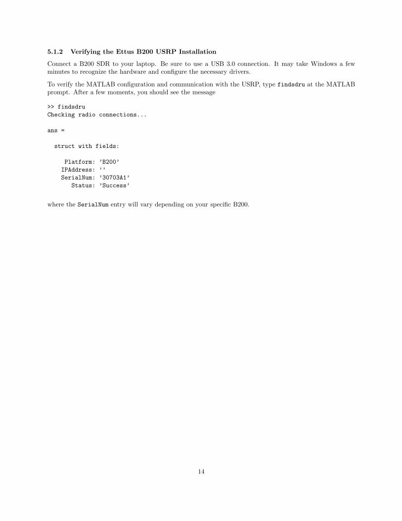
5.1.2 Verifying the Ettus B200 USRP Installation

Connect a B200 SDR to your laptop. Be sure to use a USB 3.0 connection. It may take Windows a fewminutes to recognize the hardware and configure the necessary drivers.

To verify the MATLAB configuration and communication with the USRP, type findsdru at the MATLABprompt. After a few moments, you should see the message

>> findsdru

Checking radio connections...

ans =

struct with fields:

Platform: ’B200’

IPAddress: ’’

SerialNum: ’30703A1’

Status: ’Success’

where the SerialNum entry will vary depending on your specific B200.

14

6 DSB-LC Transmitter

In this portion of the laboratory you will construct a DSB-LC transmitter using the USRP hardware. Anyonein the laboratory will be able to receive and listen to your transmission!

Just like radio-frequency transmissions in the real-world, care must be taken to ensure that users do notinterfere with each other. Therefore, each team of students will be assigned a carrier frequency and a channelbandwidth for their transmission. Make sure your transmission does not exceed your allotted portion of theradio-frequency spectrum!

The following sections will lead you through the development of your transmitter.

6.1 Using MATLAB to generate the baseband DSB-LC signal

We will use MATLAB to generate the baseband waveform, [A + m(t)], for the DSB-LC transmission. Thebaseband waveform will be sent to the USRP hardware, which will in turn translate it to the assigned carrierfrequency. A mathematical model for the SDR transmitter is presented in Appendix B.

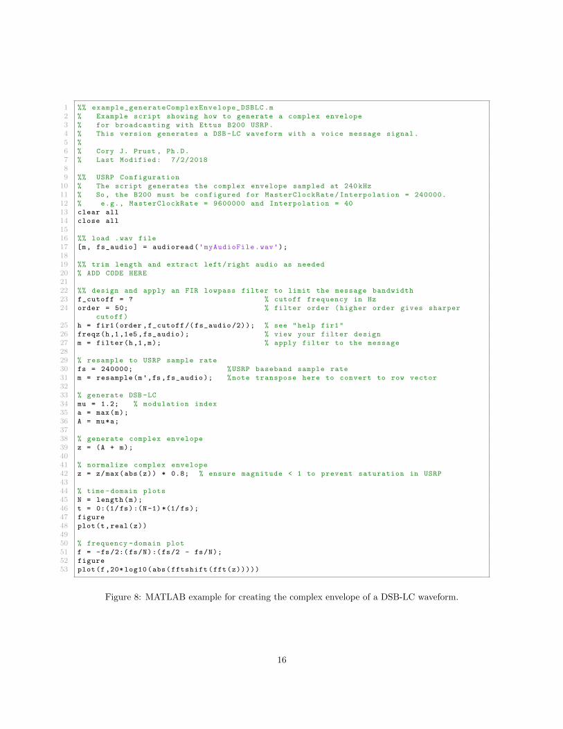
Create a MATLAB script that generates the baseband DSB-LC waveform:

1. Select a voice or audio file that you wish to transmit. Please do not use anything with objectionablecontent, such as a song containing profanity. If you have difficulties finding something to broadcast,consult your instructor.

2. Use the audioread function to load the audio file into MATLAB. The function will also return thesample rate. Be sure to make note of it. If the audio file contains stereo audio, use just the left or rightaudio signal (or sum left and right channels together). Limit the length of the audio clip to no morethan 20 seconds.

3. Your DSB-LC transmission should not exceed the channel bandwidth assigned by your instructor.Filter your message signal in accordance with your bandwidth allocation.

4. Generate the DSB-LC waveform by adding the DC offset A. You may use a modulation index of yourchoosing.

5. Normalize the amplitudes of baseband signal. For best compatibility with the USRP, all samples inthe data vector should be in the range [0, 0.9]. Plot your vector in MATLAB to ensure you have aproper DSB-LC baseband message and that the amplitude scaling is correct.

6. Resample the data vector to a sampling rate of 240000 samples per second using the resample functionin MATLAB. This is the sample rate at which data will stream across the USB interface into the USRPhardware.

Use the MATLAB Help information and the example script in Figure 8.

15

1 %% example_generateComplexEnvelope_DSBLC.m

2 % Example script showing how to generate a complex envelope

3 % for broadcasting with Ettus B200 USRP.

4 % This version generates a DSB -LC waveform with a voice message signal.

5 %

6 % Cory J. Prust , Ph.D.

7 % Last Modified: 7/2/2018

89 %% USRP Configuration

10 % The script generates the complex envelope sampled at 240 kHz

11 % So, the B200 must be configured for MasterClockRate/Interpolation = 240000.

12 % e.g., MasterClockRate = 9600000 and Interpolation = 40

13 clear all

14 close all

1516 %% load .wav file

17 [m, fs_audio] = audioread('myAudioFile.wav');

1819 %% trim length and extract left/right audio as needed

20 % ADD CODE HERE

2122 %% design and apply an FIR lowpass filter to limit the message bandwidth

23 f_cutoff = ? % cutoff frequency in Hz

24 order = 50; % filter order (higher order gives sharper

cutoff)

25 h = fir1(order ,f_cutoff /( fs_audio /2)); % see "help fir1"

26 freqz(h,1,1e5,fs_audio); % view your filter design

27 m = filter(h,1,m); % apply filter to the message

2829 % resample to USRP sample rate

30 fs = 240000; %USRP baseband sample rate

31 m = resample(m',fs ,fs_audio); %note transpose here to convert to row vector

3233 % generate DSB -LC

34 mu = 1.2; % modulation index

35 a = max(m);

36 A = mu*a;

3738 % generate complex envelope

39 z = (A + m);

4041 % normalize complex envelope

42 z = z/max(abs(z)) * 0.8; % ensure magnitude < 1 to prevent saturation in USRP

4344 % time -domain plots

45 N = length(m);

46 t = 0:(1/fs):(N-1) *(1/fs);

47 figure

48 plot(t,real(z))

4950 % frequency -domain plot

51 f = -fs/2:(fs/N):(fs/2 - fs/N);

52 figure

53 plot(f,20* log10(abs(fftshift(fft(z)))))

Figure 8: MATLAB example for creating the complex envelope of a DSB-LC waveform.

16

6.2 Creating the Simulink model

1. Open a new Simulink model and create the model shown in Figure 9.

� SDRu Transmitter (found in Communications System Toolbox Support Package for USRP).Configure exactly as shown in Figure 10. This block will act as a signal sink operating at 240000complex samples per second.

� Signal From Workspace (found in DSP System Toolbox → Sources)

– Specify signal z (or whatever name you used for your baseband message)

– Sample time: 1/240e3

– Samples per frame: 1000

– Form output after final data value by: Cyclic repetition

Figure 9: Simulink model for the DSB-LC transmitter.

2. Set the Simulation stop time to inf.

3. Temporarily comment out the SDRu Transmitter block.

4. Begin execution by clicking the play button (Run). Carefully examine the spectrum of your DSB-LCwaveform in the Spectrum Analyzer window and verify that it is as expected. In particular, confirmthat it matches your bandwidth allocation.

5. Stop your simulation. Uncomment the SDRu Transmitter block. Click Run. In a few moments, youwill be broadcasting your waveform in the laboratory!

6. Ask a lab-mate or your instructor to tune their DSB-LC receiver to your broadcast. Can you hear theresulting audio?

7. If the received signal is weak or noisy, you may need to increase the transmit gain. Under nocircumstances should you increase this setting beyond 55 dB.

17

Figure 10: SDRu block configuration for DSB-LC transmitter.

Question 6.1: Submit a time-domain plot of your baseband message signal generated inMATLAB. Scale the time axis so that the key characteristics of the waveform are clearly visible.Provide a brief explanation of what is seen in the plot.

Question 6.2: Submit a screen capture of the spectrum analyzer window showing yourtransmitted DSB-LC communication signal as it is being received on a lab-mate’s personal SDRreceiver. Provide a brief explanation of what is seen in the plot.

18

A Amplitude Modulation

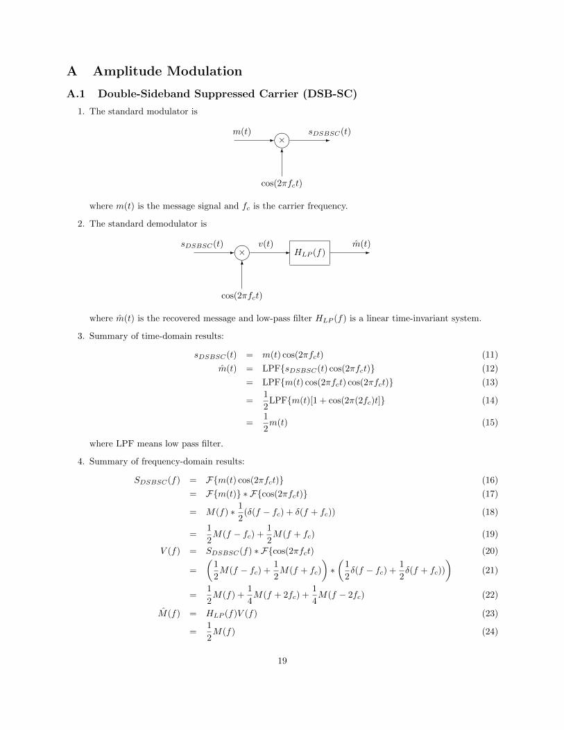
A.1 Double-Sideband Suppressed Carrier (DSB-SC)

1. The standard modulator is

-m(t) � ��

×6

cos(2πfct)

-sDSBSC(t)

where m(t) is the message signal and fc is the carrier frequency.

2. The standard demodulator is

-sDSBSC(t) � ��

×6

cos(2πfct)

-v(t)

HLP (f) -m(t)

where m(t) is the recovered message and low-pass filter HLP (f) is a linear time-invariant system.

3. Summary of time-domain results:

sDSBSC(t) = m(t) cos(2πfct) (11)

m(t) = LPF{sDSBSC(t) cos(2πfct)} (12)

= LPF{m(t) cos(2πfct) cos(2πfct)} (13)

=1

2LPF{m(t)[1 + cos(2π(2fc)t]} (14)

=1

2m(t) (15)

where LPF means low pass filter.

4. Summary of frequency-domain results:

SDSBSC(f) = F{m(t) cos(2πfct)} (16)

= F{m(t)} ∗ F{cos(2πfct)} (17)

= M(f) ∗ 1

2(δ(f − fc) + δ(f + fc)) (18)

=1

2M(f − fc) +

1

2M(f + fc) (19)

V (f) = SDSBSC(f) ∗ F{cos(2πfct) (20)

=

(1

2M(f − fc) +

1

2M(f + fc)

)∗(

1

2δ(f − fc) +

1

2δ(f + fc))

)(21)

=1

2M(f) +

1

4M(f + 2fc) +

1

4M(f − 2fc) (22)

M(f) = HLP (f)V (f) (23)

=1

2M(f) (24)

19

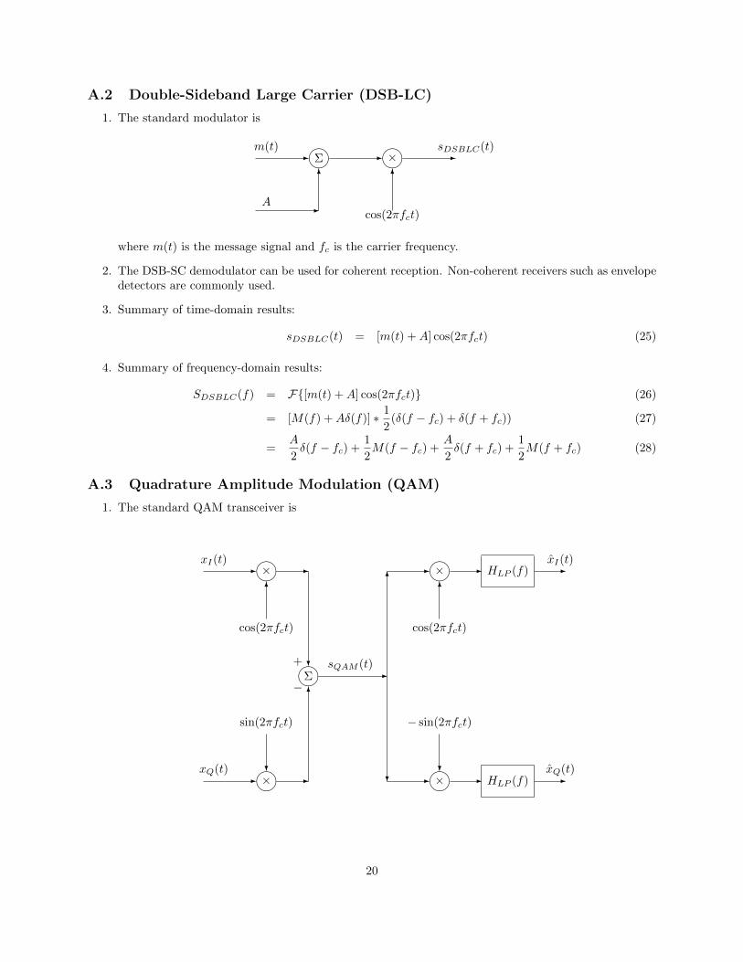
A.2 Double-Sideband Large Carrier (DSB-LC)

1. The standard modulator is

-m(t) � ��

Σ

A -

6

-� ��×6

cos(2πfct)

-sDSBLC(t)

where m(t) is the message signal and fc is the carrier frequency.

2. The DSB-SC demodulator can be used for coherent reception. Non-coherent receivers such as envelopedetectors are commonly used.

3. Summary of time-domain results:

sDSBLC(t) = [m(t) +A] cos(2πfct) (25)

4. Summary of frequency-domain results:

SDSBLC(f) = F{[m(t) +A] cos(2πfct)} (26)

= [M(f) +Aδ(f)] ∗ 1

2(δ(f − fc) + δ(f + fc)) (27)

=A

2δ(f − fc) +

1

2M(f − fc) +

A

2δ(f + fc) +

1

2M(f + fc) (28)

A.3 Quadrature Amplitude Modulation (QAM)

1. The standard QAM transceiver is

-xI(t) � ��

×6

cos(2πfct)

-

?� ��Σ

+

−6

-sQAM (t)

-xQ(t) � ��

×?

sin(2πfct)

-

6-� ��×6

cos(2πfct)

- HLP (f) -xI(t)

? -� ��×?

− sin(2πfct)

- HLP (f) -xQ(t)

20

2. Summary of time-domain results:

sQAM (t) = xI(t) cos(2πfct)− xQ(t) sin(2πfct) (29)

sQAM (t) cos(2πfct) = xI(t) cos2(2πfct)− xQ(t) sin(2πfct) cos(2πfct) (30)

= xI(t)1

2[1 + cos(2π(2fc)t)]− xQ(t)

1

2[sin(2π(2fc)t) + sin(0)] (31)

=1

2xI(t)[1 + cos(2π(2fc)t)]−

1

2xQ(t) sin(2π(2fc)t) (32)

−sQAM (t) sin(2πfct) = −xI(t) cos(2πfct) sin(2πfct) + xQ(t) sin2(2πfct) (33)

= −xI(t)1

2[sin(2π(2fc)t) + sin(0)] + xQ(t)

1

2[1− cos(2π(2fc)t)] (34)

= −1

2xI(t) sin(2π(2fc)t) +

1

2xQ(t)[1− cos(2π(2fc)t)] (35)

(36)

Therefore

xI(t) = LPF{sQAM (t) cos(2πfct)} (37)

=1

2xI(t) (38)

xQ(t) = LPF{−sQAM (t) sin(2πfct)} (39)

=1

2xQ(t) (40)

(41)

21

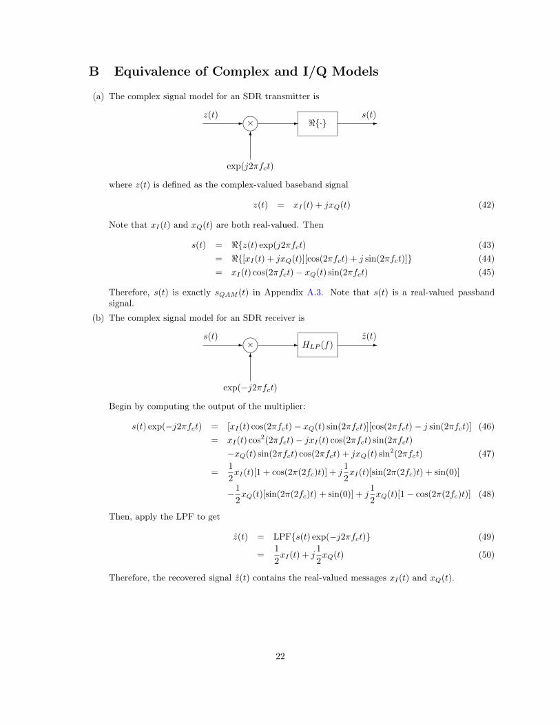
B Equivalence of Complex and I/Q Models

(a) The complex signal model for an SDR transmitter is

-z(t) � ��

×6

exp(j2πfct)

- <{·} -s(t)

where z(t) is defined as the complex-valued baseband signal

z(t) = xI(t) + jxQ(t) (42)

Note that xI(t) and xQ(t) are both real-valued. Then

s(t) = <{z(t) exp(j2πfct) (43)

= <{[xI(t) + jxQ(t)][cos(2πfct) + j sin(2πfct)]} (44)

= xI(t) cos(2πfct)− xQ(t) sin(2πfct) (45)

Therefore, s(t) is exactly sQAM (t) in Appendix A.3. Note that s(t) is a real-valued passbandsignal.

(b) The complex signal model for an SDR receiver is

-s(t) � ��

×6

exp(−j2πfct)

- HLP (f) -z(t)

Begin by computing the output of the multiplier:

s(t) exp(−j2πfct) = [xI(t) cos(2πfct)− xQ(t) sin(2πfct)][cos(2πfct)− j sin(2πfct)] (46)

= xI(t) cos2(2πfct)− jxI(t) cos(2πfct) sin(2πfct)

−xQ(t) sin(2πfct) cos(2πfct) + jxQ(t) sin2(2πfct) (47)

=1

2xI(t)[1 + cos(2π(2fc)t)] + j

1

2xI(t)[sin(2π(2fc)t) + sin(0)]

−1

2xQ(t)[sin(2π(2fc)t) + sin(0)] + j

1

2xQ(t)[1− cos(2π(2fc)t)] (48)

Then, apply the LPF to get

z(t) = LPF{s(t) exp(−j2πfct)} (49)

=1

2xI(t) + j

1

2xQ(t) (50)

Therefore, the recovered signal z(t) contains the real-valued messages xI(t) and xQ(t).

22

References

[1] Ettus Research LLC. Ettus research - home. http://www.ettus.com.

[2] Ettus Research LLC. UHD start. http://code.ettus.com/redmine/ettus/projects/uhd/wiki.

[3] Ettus Research LLC. Ettus research - usrp b200 software defined radio.http://www.ettus.com/product/details/UB200-KIT.

[4] Ettus Research LLC. Usrp hardware driver and usrp manual. http://files.ettus.com/manual/.

[5] Mathworks. Communications Toolbox. Online Resource. https://www.mathworks.com/products/communications.html.

[6] Mathworks. USRP Support Package from Communications Toolbox. Online Resource.http://www.mathworks.com/discovery/sdr/usrp.html.

[7] Mathworks. RTL-SDR Support Package from Communications Toolbox. Online Resource.https://www.mathworks.com/hardware-support/rtl-sdr.html.

[8] Leon W. Couch III. Digital and Analog Communication Systems. 7th edition, 2007.

[9] Simon Haykin. Communication Systems. 4th edition, 2001.

23