Embed Size (px)
Citation preview

arX
iv:0
911.
2403
v2 [
phys
ics.
flu-
dyn]
31
Mar
201
0APS/123-QED
Destabilizing Taylor-Couette flow with suction
Basile Gallet∗
Laboratoire de physique statistique, Ecole Normale Superieure, 75231 Paris France
Charles R. Doering
Department of Mathematics, Department of Physics, and Center for the Study of
Complex Systems, University of Michigan, Ann Arbor 48109-1043 USA
Edward A. Spiegel
Department of Astronomy, Columbia University, New York NY 10027 USA
(Dated: October 29, 2018)
Abstract
We consider the effect of radial fluid injection and suction on Taylor-Couette flow.
Injection at the outer cylinder and suction at the inner cylinder generally results in
a linearly unstable steady spiralling flow, even for cylindrical shears that are linearly
stable in the absence of a radial flux. We study nonlinear aspects of the unstable
motions with the energy stability method. Our results, though specialized, may
have implications for drag reduction by suction, accretion in astrophysical disks,
and perhaps even in the flow in the earth’s polar vortex.
∗Electronic address: [email protected]
1

I. THE PROBLEM
There are many contexts in which rotating flows arise and their instabilities are naturally
of interest. For an axisymmetric, incompressible, inviscid flow with no variation along the
axis of symmetry, Rayleigh (1916) provided a necessary and sufficient condition for stability
against axisymmetric perturbations (Chandrasekhar, 1961). Rayleigh also showed that a
necessary criterion for the instability of such flows to non-axisymmetric perturbations is an
analogue to his classic inflection point criterion for plane flows. He expressed this criterion
in words but the correct mathematical expression is easily worked out following Rayleigh’s
lead (Spiegel and Zahn, 1970). For the study of the effect of viscosity on these results,
the Taylor-Couette configuration of flow between coaxial cylinders provides a good proving
ground (Chandrasekhar, 1961), although shear and rotation come together in other contexts
as well (Yecko and Rossi, 2004 and references therein).
When criteria for the simplest two-dimensional circular shear flows indicate stability, the
question naturally arises whether some simple extraneous effects may be destabilizing. In
the case of the linearly stable plane shear flow, magnetic fields (Stern, 1963 and Chen and
Morrison, 1991), Rossby waves (Lovelace et al., 1999) and suction (Hocking, 1974; Doering
et al., 2000) have been found to be destabilizing mechanisms, given suitable conditions. In
the case of a stable Taylor-Couette flow, it had been seen even earlier that a magnetic field
may be destabilizing (e.g. Chandrasekhar, 1961; Balbus and Hawley, 1998). In an attempt
to add to this compendium of instabilities, we here investigate the instability that arises
when a formerly circular flow is turned into a spiralling flow by the imposition of continous
suction on the inner cylindrical boundary with a compensatory injection of fluid on the outer
boundary. For brevity, we shall hereinafter refer to the induced radial inflow as accretion
and the mechanism driving it as suction.
A practical example of the conversion of differential circular flow to spiraling motion, or
swirl, arises in the study of drag reduction on a cylindrical airfoil (Batchelor, 1967). In that
case, when suction is imposed on the central cylindrical airfoil, the drag is reduced because
boundary layer separation is inhibited. Spiralling flows are also central to the structure and
dynamics of accretion disks that form in a great variety of astrophysical situations such as
binary stars (which are often X-ray sources), flows around massive black holes at the centers
of galaxies, and in the disks around newly born stars where planetary systems are thought
2

to form.
Of course, accretion disks are more complicated than the simple model that we consider
here. In most astrophysical cases there is ionization so hydromagnetic effects become im-
portant and can produce the magneto-rotational instability (see Balbus and Hawley, 1998).
However, protoplanetary nebulae such as the primitive solar nebula are believed to have
been cool so that other mechanisms may need to be considered to get the full picture (for
at least some phases) of the turbulent dynamics of planet formation. The feature of the
present study that may have relevance to the fluid dynamics of astrophysical disks is the
radial inflow, or accretion that, in some astrophysical examples, is fed by inflow from an
external mass source. A similar combination of motions occurs also in the terrestrial polar
vortex that may play a role in the transport of ozone in the upper atmosphere (McIntyre,
1995).
With these motivational examples in mind, we turn to an idealized pilot problem to learn
what may happen when rotation and accretion combine to produce a spiralling motion as in
Taylor-Couette flow with suction. Although we cannot draw immediate conclusions about
the applications of our results to the motivational examples just described, especially to
accretion disks, we regard it as suggestive that the combination of rotation and accretion
(i.e., radial injection and suction) in a flow leads to instability. As we shall see in what
follows, taking into account both accretion and rotation leads to very different stability
properties of the flow than when only one of these effects alone is included. For example,
in the classical problem of the linear and nonlinear stability of Taylor-Couette flow between
concentric cylinders, the system is linearly stable when the outer cylinder is rotating and the
inner one is stationary. Likewise, simple radial accretion without rotation is linearly stable.
However, we find that, at sufficiently large rotational Reynolds numbers in a stable TC flow,
small accretion rates lead to linear instability. Moreover we find that the rotational motion,
rather than simple plane shear, plays a major role in the stability characteristics.
An initially plane-parallel shear layer perturbed by transverse suction may also exhibit a
small-suction instability (Hocking, 1974), while larger suction rates absolutely stabilize the
corresponding laminar flow for arbitrarily large Reynolds numbers (Doering et al., 2000).
This strong stabilizing effect of suction for even very high Reynolds numbers in the plane
case does not carry over to the rotational case; in the cylindrical geometry transient growth
of perturbations is generally encouraged by strong suction.
3

The following discussion of these issues is organized as follows. In section II we describe
Taylor-Couette flow with suction. Then we treat the linear stability of this flow in section
III where we find linear instabilities in the simple flow of the model problem. In section
IV the asymptotic behavior of the onset of linear instability is computed for different limits
in the narrow-gap approximation. We next go on to consider some nonlinear aspects of
the instability. First, in section V we describe the energy stability method and then derive
some rigorous bounds on the energy stability limit of the flow in section VI. That limit is
computed numerically in section VII. The concluding section VIII summarizes the results
and mentions some possible implications. In an appendix we note that physically relevant
bounds on the mean energy dissipation rate for non-steady flows (including statistically
stationary turbulence) remain unknown in the Taylor-Couette geometry with suction.
II. FORMULATION OF THE PROBLEM
A. Geometry of the problem and boundary conditions
Consider the incompressible flow of a Newtonian fluid between two coaxial porous cylin-
ders. For definiteness, we let the inner cylinder be at rest while the outer cylinder is rotating
with constant angular velocity, Ω. The radii of the inner and outer cylinders are, respec-
tively, R1 and R2, and we use cylindrical coordinates (r, θ, z). We consider periodic boundary
conditions in z with period Lz, and impose no-slip boundary conditions so that the vertical
(z) component of the velocity field vanishes at both cylinders and the azimuthal component
matches the velocity of each of the cylinders.
Now we add a radial inward flow to this classical Taylor-Couette configuration. Fluid is
injected at the outer cylinder with the constant volume flux 2πϕ (volume of fluid injected
per unit time and per unit height of cylinder) and uniformly sucked out at the inner cylinder
at the same rate. The control parameter ϕ ≥ 0 is central in what follows. The resulting
velocity field is u = uer + veθ + wez and the boundary conditions are
u(R1, θ, z) = − ϕ
R1er (1)
u(R2, θ, z) = − ϕ
R2er +R2Ωeθ. (2)
4

The incompressibility constraint ∇.u = 0 implies two further boundary conditions:
ur(R1) = 0 and ur(R2) = 0 (3)
where the subscript r denotes partial differentiation with respect to r. A schematic of the
set-up is shown in Figure 1.
R1
R2InjectionRotating
cylinder angle
FIG. 1 The outer cylinder rotates at angular velocity Ω. Fluid is injected at the outer boundary
with an entry angle Θ = arctan[ϕ/(R22Ω)], and removed uniformly on the surface of the inner
cylinder.
B. Dimensionless numbers
This problem involves five parameters: the two radii, R1 and R2, the angular velocity
of the outer cylinder, Ω, the imposed accretion flux, 2πϕ, and the viscosity of the fluid, ν.
Nondimensionalizing time and space leaves three independent dimensionless numbers η, Θ
and Re describing the geometry and physical boundary conditions:
• The geometrical factor is η = R1
R2
. When η → 1 we approach the narrow gap
limit where (R2 − R1) << R1, and expect to find results similar to those from
the slab geometry — namely plane Couette flow with suction. On the other hand,
when η goes to zero, the outer radius R2 goes to infinity relative to the inner ra-
dius and we expect to see significant effects of the curvature on the stability of the flow.
5

• The accretion flux is measured by the injection angle, Θ, at the outer cylinder, where
tanΘ =ϕ
R22Ω. (4)
If tanΘ = 0, there is no suction and we recover a classical Taylor-Couette problem
with a linearly stable stationary flow when the inner cylinder is stationary. When
tanΘ → ∞ we approach the limit where suction dominates rotation.
• The azimuthal Reynolds number is
Re =R2Ω(R2 −R1)
ν=R2
2Ω(1− η)
ν. (5)
We choose this definition of the Reynolds number to match the definition of the
Reynolds number for the plane Couette flow when η → 1.
• Introduction of an additional parameter, the radial Reynolds number α = ϕ/ν, is use-
ful for making some of the equations more compact. This parameter is not independent
but is linked to Re, η and tan(Θ) by the relation
α =Re tanΘ
1− η. (6)
We define the dimensionless velocity u = uer+ veθ+wez = u/(R2Ω) and the dimension-
less coordinates r = r/R2 and z = z/R2 and the time t = Ωt . The velocity field satisfies
the incompressible Navier-Stokes equations, written in dimensionless form as
ut + u · ∇u = −∇p+ 1− η
Re∆u (7)
with boundary conditions
u(η, θ, z, t) = −tanΘ
ηer (8)
u(1, θ, z, t) = −tanΘ er + eθ (9)
ur(η, θ, z, t) = 0 (10)
ur(1, θ, z, t) = 0 (11)
6

C. The basic laminar solution
The basic steady laminar solution Vlam = (U(r), V (r), 0) of equation (7) has radial
velocity
U(r) = −tanΘ
r(12)
and azimuthal velocity
V (r) =1
1− η2−αr1−α +
1
1− ηα−2
1
r. (13)
The azimuthal velocity profile is represented in Figure 2 for several different combinations
of values of α and η.
When α → 0 we recover the classical velocity field of the Taylor-Couette flow with a
stationary inner cylinder. That flow is independent of the kinematic viscosity, ν, and the
azimuthal velocity then increases monotonically when r increases from η to 1.
For nonzero values of the entry angle tanΘ and for sufficiently large values of the Reynolds
number, that is, for Re tanΘ >> 1, the azimuthal speed increases outward (from the inner
boundary) in a boundary layer of thickness δ. On the other hand, as the fluid comes in from
the outer boundary, its motion is mostly inviscid and thus conserves angular momentum
rV (r): the azimuthal velocity of the fluid element increases during the inward journey from
the outer boundary according to
V (r) ≈ 1
r(14)
For α > 1, the two flows join to form an azimuthal velocity profile with a maximum at
r = η + δ:
Vr(η + δ) = 0 ⇔ δ = η[(α− 1)1
α−2 − 1]. (15)
This particular feature of the azimuthal velocity profile, that it can achieve a local maximum
within the gap for α > 1, is fundamentally linked to the rotational geometry. This effect
disappears in the plane limit η → 1 since the maximum value of the azimuthal velocity
inside the gap Vmax =1η. For large values of α, the boundary layer is very thin; δ ∼ η ln(α)
α.
These considerations point up a significant but not widely appreciated feature of accre-
tion flows. The asymptotic velocity profile as Re → ∞ is dramatically modified from its
7

structure at tanΘ = 0 when tanΘ 6= 0. When tanΘ = 0, the azimuthal velocity profile is
the Reynolds-number-independent Taylor-Couette profile. When tanΘ 6= 0 the azimuthal
velocity profile varies as 1reverywhere inside the gap and outside the boundary layer, which
becomes infinitely thin in the limit Re → ∞. This shows that even if the accretion rate
is very low (but not zero), one cannot neglect it at high Re and study the problem with
rotation only. The limits Re→ ∞ and tanΘ → 0 do not commute.
0 0.5 1 1.50.9
0.92
0.94
0.96
0.98
1
V
r
α=0α=1α=10α=100
0 0.5 1 1.5 20.5
0.6
0.7
0.8
0.9
1
V
r
α=0α=1α=10α=100
FIG. 2 Azimuthal velocity profiles for different values of the radial Reynolds number (top : η = 0.9,
bottom : η = 0.5).
8

III. LINEAR STABILITY ANALYSIS AND NON-AXISYMMETRIC DISTUR-
BANCES
To study the destabilizing effect of the inward suction on the stability properties of Taylor-
Couette flow, we perform a linear stability analysis. It is already known from work by Min
and Lueptow (1994) that, for axisymmetric disturbances to Taylor-Couette flow, suction is
stabilizing and so increases the critical Taylor number at which Taylor vortices first appear.
Therefore we here consider the linear stability theory for non-axisymmetric perturbations.
We continue to keep the inner cylinder stationary, so that the flow without suction is linearly
stable according to Rayleigh’s criteria for inviscid perturbations.
In most instability mechanisms, only one symmetry of the initial problem is broken at the
onset of the primary instability while others are broken through secondary instabilities. Since
we anticipate instability to nonaxisymmetric perturbations, we shall not, in the first instance,
break the invariance to translations in the z-direction in seeking the primary instabilities of
the spiralling flow. We observe that, consistently with this supposition, a Squire’s Theorem
exists in the plane-shear-with-suction situation, that is, in the limit η → 1 (Doering et al.,
2000).
A. Linearization of the equations
We make the decomposition u = Vlam + v for the full velocity field, write the r, θ, and
z components of a mode of the perturbation as
v = (u(r), v(r), 0)e−λteimθ (16)
and seek the (possibly complex) eigenvalue λ. The linearized versions of the Navier-Stokes
equations for the r and θ components of v for this mode are
λu = −1− η
Reurr −
tanΘ + 1−ηRe
rur + A1u+ Z1v + pr (17)
λv = −1− η
Revrr −
tanΘ + 1−ηRe
rvr + A2v + Z2u+
imp
r(18)
9

where p is the pressure perturbation and
A1 = imV
r+
tanΘ
r2+
1− η
Re
m2 + 1
r2, (19)
A2 = imV
r− tanΘ
r2+
1− η
Re
m2 + 1
r2, (20)
Z1 =(1− η)
Re
2im
r2− 2V
r, and (21)
Z2 = Vr +V
r− (1− η)
Re
2im
r2. (22)
The continuity equation becomes
imv + (ru)r = 0, (23)
providing an expression for v that may be inserted into (18) to give p in terms of u. Then,
upon differentiating p with respect to r and inserting the result into (17), we arrive at a
fourth order ODE for u(r):
λ[
−r2urr − 3rur + (m2 − 1)u]
=
[
(1− η)
Rer2]
urrrr (24)
+
[(
6(1− η)
Re+ tanΘ
)
r
]
urrr +
[
(1− η)
Re(6−m2) + 3 tanΘ− r2A2
]
urr
+
[
−tanΘ + (1−η)Re
rm2 + imrZ1 + imrZ2 − r2(A2)r − 3rA2
]
ur
+[
m2A1 + imZ1 + imZ2 + imr(Z2)r − r(A2)r − A2
]
u.
The boundary conditions are that u and ur vanish at r = η and r = 1.
10

10−3
10−2
10−1
102
104
106
tan(θ)
Re
m=1
m=3
m=30
m=10
m=100
10−4
10−3
10−2
10−1
100
1
1.05
1.1
1.15
1.2
1.25
tan(θ)
Im(λ
)/m
x
y
−0.3 −0.2 −0.1 0 0.1 0.2 0.3
0.85
0.9
0.95
1
xy
−0.3 −0.2 −0.1 0 0.1 0.2 0.3
0.85
0.9
0.95
1
FIG. 3 Top: Linear stability limit of several modes for η = 0.9 (left) and angular velocity of
propagation of the unstable mode at onset (right). Thick dashed line : m = 1; dashed line :
m = 3; dash-dotted line : m = 10; solid line : m = 30; dotted line : m = 100. The energy
stability limit has been added to make the comparison easier (thick solid line). Bottom: Contour
plot of the streamfunction of the unstable mode at the onset of instability for m = 10, η = 0.9,
and tanΘ = 0.001 (left) and tanΘ = 0.01 (right). The smaller the injection angle, the more the
velocity gradients are pressed up against the injection boundary.
11

B. Numerical computation of the linear stability limit
Equation (24) presents an eigenvalue problem which can be solved numerically using a
standard finite difference method. The linear stability limit of different modes is represented
in Figures 3 and 4 for η = 0.9 and η = 0.5. There is linear instability even at small injection
angles. The modes that become unstable for the lowest critical Reynolds number have
m ∼ 11−η
, corresponding to closed and almost circular cells (in the (r, θ) plane) between the
two cylinders. As expected for a system that lacks reflection symmetry in the θ-direction,
the unstable mode is a travelling wave that propagates in the azimuthal direction. The
angular velocity of propagation Im(λ)/m at the onset of instability is plotted in Figures 3
and 4.
At a certain value of the injection angle, the linear stability boundary has a vertical
asymptote in the tanΘ−Re plane (see Figure 3). Above this critical value of the injection
angle, the flow is linearly stable at any Reynolds number. Comparing the linear stability
limits obtained for the two values of η, we notice that the flow is more unstable linearly for
the geometry with the highest curvature. From η = 0.9 to η = 0.5, the minimum value of
the Reynolds number for marginal stability — the critical Reynolds number — goes from
approximately 104 to 2 × 10³ and the maximum value of the injection angle that allows a
linear instability increases by almost an order of magnitude. A few plots of the unstable
modes at the onset of instability are presented in Figures 3 and 4. Close to the critical
injection angle the cells occupy the full width of the gap, whereas for smaller values of
the injection angle the modes are pressed up against the injection boundary. In this latter
situation, the angular velocity of propagation tends to 1, corresponding to the unstable mode
being advected by the flow at the dimensionful angular velocity Ω of the outer boundary.
As already remarked, these linear instabilities exist when both rotation and accretion are
present but they are lost if only one of these two ingredients is present in the configuration
considered here.
IV. NARROW-GAP LIMIT
Since the numerical problem is readily solved in the linear case, we have the luxury of
using some rough and ready approximation methods to extract analytic results about linear
12

10−3
10−2
10−1
101
102
103
104
105
tan(θ)
Re
10−3
10−2
10−1
100
1
1.5
2
2.5
3
tan(θ)
Im(λ
)/m
x
y
−1 −0.5 0 0.5 1−1
−0.5
0
0.5
1
x
y
−1 −0.5 0 0.5 1−1
−0.5
0
0.5
1
FIG. 4 Top: Linear stability limit of several modes for η = 0.5 (left) and angular velocity
of propagation of the unstable mode at onset (right). In this high curvature geometry, linear
instability is found for lower values of the Reynolds number and up to higher values of the injection
angle. Solid line: m = 1; dashed line: m = 2; dashed-dotted line: m = 3; dotted line: m = 4; thick
solid line: energy stability limit. Bottom left: Contour plot of the streamfunction of the unstable
mode at the onset of instability for m = 2, η = 0.5, and tanΘ = 0.005. The streamlines are
concentrated toward the injection boundary. Bottom right: Contour plot of the streamfunction
of the unstable mode at the onset of instability for m = 2, η = 0.5 and tanΘ = 0.1. The cells
occupy the whole gap.
13
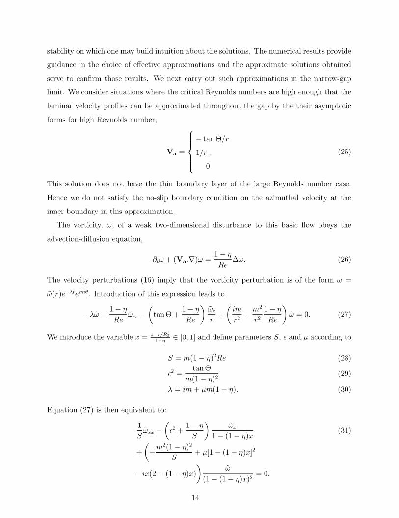
stability on which one may build intuition about the solutions. The numerical results provide
guidance in the choice of effective approximations and the approximate solutions obtained
serve to confirm those results. We next carry out such approximations in the narrow-gap
limit. We consider situations where the critical Reynolds numbers are high enough that the
laminar velocity profiles can be approximated throughout the gap by the their asymptotic
forms for high Reynolds number,
Va =
− tanΘ/r
1/r .
0
(25)
This solution does not have the thin boundary layer of the large Reynolds number case.
Hence we do not satisfy the no-slip boundary condition on the azimuthal velocity at the
inner boundary in this approximation.
The vorticity, ω, of a weak two-dimensional disturbance to this basic flow obeys the
advection-diffusion equation,
∂tω + (Va.∇)ω =1− η
Re∆ω. (26)
The velocity perturbations (16) imply that the vorticity perturbation is of the form ω =
ω(r)e−λteimθ. Introduction of this expression leads to
− λω − 1− η
Reωrr −
(
tanΘ +1− η
Re
)
ωrr
+
(
im
r2+m2
r21− η
Re
)
ω = 0. (27)
We introduce the variable x = 1−r/R2
1−η∈ [0, 1] and define parameters S, ǫ and µ according to
S = m(1 − η)2Re (28)
ǫ2 =tanΘ
m(1 − η)2(29)
λ = im+ µm(1− η). (30)
Equation (27) is then equivalent to:
1
Sωxx −
(
ǫ2 +1− η
S
)
ωx1− (1− η)x
(31)
+
(
−m2(1− η)2
S+ µ[1− (1− η)x]2
−ix(2 − (1− η)x)
)
ω
(1− (1− η)x)2= 0.
14

In the narrow gap limit of this equation, for which (1− η)x≪ 1, we find
1
Sωxx −
(
ǫ2 +1− η
S
)
ωx +
(
−m2(1− η)2
S+ µ− 2ix
)
ω = 0. (32)
A. Linear stability limit for small injection angles
As we saw, instability requires both rotation (the first term of (32)), and accretion (the
term proportional to ǫ2). Hence we require that the three terms of equation (32) are of the
same order of magnitude within the active layer, the layer close to the injection boundary
(x = 0) where the main development of the unstable mode occurs for small injection angles.
We bring this out by introducing the scalings
S =N
ǫ3, µ = ǫa and x = ǫy, (33)
with N , a and y all O(1) inside the boundary layer. Equation (32) then becomes
1
Nωyy − ωy + (a− 2iy)ω = O(ǫ) (34)
We are interested only in the leading order behavior in ǫ, so we discard the right hand
side, which is proportional to ǫ. In the narrow-gap limit, the vorticity is linked to the
streamfunction ψ of the perturbation by
ω ≃ −ψrr +m2ψ =1
(1− η)2
(
−ψyyǫ2
+m2(1− η)2ψ
)
. (35)
Hence, at the leading order in ǫ, ω may be replaced in (34) by ψyy . Thus the streamfunction
close to the boundary satisfies
1
Nψyyyy − ψyyy + (a− 2iy)ψyy = 0. (36)
The solution for ψyy that vanishes for large y can be expressed in terms of the Airy function:
ψyy(y) = eN2yAi
(
−N1/3a
(2i)2/3+
N4/3
4(2i)2/3+ (2i)1/3N1/3y
)
. (37)
If we let ψin denote the corresponding solution that vanishes for large y, i.e., the inner
solution, we can write the general solution as
ψ(y) = Ay +B + ψin(y). (38)
15

0 2 4 6 8−0.2
0
0.2
0.4
0.6
0.8
1
1.2
y
ψ in
FIG. 5 Inner solution at the onset of instability N = Nc = 4.58 and a = 5.62i (solid line: real
part, dashed line: imaginary part).
The boundary condition ψ(1ǫ) = 0 gives Ay + B = A(y − 1
ǫ). The boundary condition
ψ(0) = 0 leads to A = ǫψin(0) and, finally, the boundary condition ψy(0) = 0 gives ǫψin(0)+
(dψin
dy)y=0 = 0. In the limit ǫ → 0 this relation becomes (dψin
dy)y=0 = 0. The parameter a is
then a solution of the implicit equation∫ ∞
0
eN2yAi
(
−N1/3a
(2i)2/3+
N4/3
4(2i)2/3+ (2i)1/3N1/3y
)
dy = 0. (39)
The onset of instability is found for N = Nc so that a is purely imaginary. We get the
critical values Nc ≃ 4.58 and a = 5.62i. The asymptotic behavior for small values of the
injection angle then corresponds to
Rec ∼ 4.58m1/2(1− η) tanΘ−3/2,
Im(λ) = m+ 5.62√
m tan(θ). (40)
The imaginary part of the eigenvalue corresponds to the advection of the pattern by the mean
flow close to the outer boundary: for small injection angles, the eigenmode is a traveling
wave of dimensionful angular velocity Ω. The inner solution at the onset of instability is
represented in Figure 5.
B. Critical injection angle for the smallest azimuthal wavenumbers
Close to the critical injection angle for which the critical Reynolds number goes to infinity,
the instability develops in the whole width of the gap. The parameter ǫ does not necessarily
16

0 0.2 0.4 0.6 0.8 1−2
−1
0
1
2
3
4
x
ψ
FIG. 6 Marginally stable mode at the onset of instability ǫ2c = 0.166 and µ = 2.04i, for an infinite
Reynolds number (solid line: real part, dashed line: imaginary part).
have to be small, but we simplify our calculations by focusing on the lowest of the azimuthal
wavenumbers — specifically on m2(1−η)2 ≪ 1. At the leading order in m2(1−η)2, equation(35) reduces to
ω = − ψxx(1 − η)2
. (41)
Inserting this into (32) and taking the limit S → ∞ gives
ǫ2ψxxx + (2ix− µ)ψxx = 0 (42)
with solution
ψxx = exp
(
1
ǫ2(µx− ix2)
)
. (43)
Imposing the boundary conditions ψ(0) = 0, dx(ψ)x=0 = 0, ψ(1) = 0, we deduce the
dispersion relation∫ 1
t=0
∫ t
x=0
exp
(
1
ǫ2(µx− ix2)
)
dxdt = 0. (44)
Once again, the critical injection angle is obtained when the solution µ of this implicit
equation has vanishing real part. This yields the values ǫ2c = 0.166 and µ = 2.04i, and hence
the asymptotic behavior is given by
tanΘc = 0.166m(1− η)2
Im(λ) = m+ 2.04m(1− η) (45)
The unstable mode is shown in Figure 6.
17

−3.5 −3 −2.5 −2 −1.5 −1 −0.52.5
3
3.5
4
4.5
5
log(ε2)
log(
S)
S=4.58 ε−3
εc2=0.166
−4 −3 −2 −1 00
0.5
1
1.5
2
2.5
log(ε2)
|µ|
y=5.62 ε
y(εc)=2.04
FIG. 7 Top: Curves of marginal stability for different values of η and different azimuthal wavenum-
bers m, in the ǫ2 − S plane. The small injection-angle asymptote is valid for every curve in the
small gap limit. There is always a vertical asymptote but its placement is accurate for small
wavenumbers only (m2(1 − η)2 << 1). Bottom: (Rescaled) deviation of the angular velocity of
propagation to that of the outer cylinder. The asymptotic behaviors have been drawn for compar-
ison. The symbols are : η = 0.9, m = 3; : η = 0.9, m = 10; ⋄: η = 0.9, m = 30; ·: η = 0.99,
m = 30; +: η = 0.99, m = 100; •: η = 0.99, m = 300.
C. Collapsing the different marginal stability curves
The marginal stability curves are plotted on Figure 7 in the ǫ2−S plane for different values
of η (in the small gap limit) and different values of the azimuthal wavenumber m. The curves
18

corresponding to the lowest azimuthal wavenumbers (in the sense that m2(1 − η)2 ≪ 1),
collapse onto a single curve. For small injection angles, this curve admits an asymptote
given by equation (40). Its critical injection angle is given by the vertical asymptote derived
in (45). For high azimuthal wavenumbers, the asymptote to the limit of small injection
angles is still acurate, but the vertical one is not. This comes from the fact that one cannot
simplify the relation ω ≃ − ψxx
(1−η)2+m2ψ, and thus cannot ignore the dimensionless parameter
m2(1− η)2 in the limit of high azimuthal wavenumbers. The critical injection angle goes to
zero in this limit, and its behavior may be determined with more careful asymptotics.
The angular velocity of propagation of the unstable modes are collapsed onto a single
master curve in Figure 7 by plotting the quantity |µ| =(
Im(λ)m
− 1)
/(1− η) as a function
of ǫ2. This quantity can be thought of as (a rescaled version of) the deviation of the angular
velocity of propagation to the velocity of the outer boundary. It goes to zero as ǫ tends
to zero following the scaling law (40), whereas it tends to the finite value 2.04 as ǫ → ǫc
according to equation (45).
V. ENERGY STABILITY OF THE BASIC FLOW
Energy stability is defined below; it is a strong form of nonlinear stability theory. It
provides sufficient conditions for a flow to be stable to perturbations of arbitrary amplitude.
However a flow that is not energy stable may still be linearly stable. In this section we
formulate the problem of determining the energy stability limit of the base flow introduced
above.
A. Evolution equation for the energy of the deviation from the laminar solution
The starting point for the analysis is the decomposition of the velocity field u into the
steady laminar flow and a time dependent deviation. In this analysis the deviation from
the laminar solution need not be small. We thus introduce the decomposition u(r, t) =
Vlam(r) + v(r, t) into equation (7) to obtain
vt + (v.∇)v + (Vlam.∇)v + (v.∇)Vlam = −∇p + 1− η
Re∆v . (46)
The time-dependent velocity field v(r, t) is divergence free, satisfies the homogeneous bound-
ary conditions v = 0 at the two cylinders, and is assumed to be periodic in z with period
19

Lz.
To study the kinetic energy of this variable field we take the dot product of this equation
with v and integrate over one cell, i.e. over the domain τ = [R1, R2]× [0, 2π]× [0, Lz]. Let
us denote the volume element in this domain by dτ and introduce the notation
||f ||2 =∫
τ
|f |2dτ
for what is known as the L2 norm of f . Then, after a few integrations by parts that make
use of the homogeneous boundary conditions on v, we have
d
dt
( ||v||22
)
= −∫
τ
[
1− η
Re|∇v|2 + v.(∇Vlam).v
]
dτ ≡ −Hv. (47)
If the quadratic form H is strictly positive, i.e., if there is a number µ > 0 such that Hv ≥µ||v||2 for any divergence-free field satisfying the homogeneous boundary conditions, then the
kinetic energy of the perturbation v decreases monotonically in time at least exponentially.
A flow for which H is a positive quadratic form is called energy stable — it possesses a strong
form of absolute asymptotic nonlinear stability.
Now we define the function µ(Re, tanΘ) by
µ(Re, tanΘ) = infHv||v||2 , (48)
the infimum (or greatest lower bound) being taken over divergence-free vector fields satisfying
the homogeneous boundary conditions. Energy stability is achieved in the region where
µ(Re, tanΘ) > 0 in the Re − tanΘ plane. The level set µ(Re, tanΘ) = 0 is the boundary
of the parameter region where the flow is marginally energy stable.
B. Euler-Lagrange equations
Only the terms of equation (46) which are linear in v contribute to H so that it is clear
that we can write Hv =∫
τv ·Lvdτ where L is a symmetric linear operator diagonalizable
in an orthonormal basis with real eigenvalues. We perform the variational procedure subject
to the constraint of incompressibility of the flow by adding the integral∫
τp∇.vdτ to H. A
second Lagrange multiplier λ is used to impose the constraint ||v||2 = constant when seeking
the infimum in equation (48). We may then seek a stationary condition on the combined
functional. The Euler-Lagrange equations are then
λv = −1− η
Re∆v +
1
2[(∇Vlam).v + v.(∇Vlam)] +∇p (49)
20

together with the incompressibility constraint ∇ · v = 0. As usual, the Lagrange multiplier,
p, in the Euler-Lagrange equations plays the role of pressure. The Euler-Lagrange equations
for the variational problem are equivalent to the eigenvalue problem for the linear operator
L and the infimum in equation (48) is reached when v is an eigenvector of L for its lowest
eigenvalue. This lowest eigenvalue is the lowest acceptable value of λ in equation (49). We
stress the fact that although these equations are linear they give sufficient conditions for the
laminar flow to be stable against perturbations of arbitrarily large amplitude. We solve this
problem numerically in VII but first we consider some analytical aspects.
In the classical Taylor-Couette flow without suction one can show that for some parameter
values, the Taylor-vortices — that is a z-dependent and θ-independent mode — are linearly
stable but may exhibit transient growth (see for instance Joseph, 1976). In the present
energy stability analysis of the Taylor-Couette flow with suction, we thus need to retain
both θ and z dependent deviation fields v to compute the energy stability limit correctly.
Since the problem is linear and invariant to translations in θ and z, it is useful to decom-
pose v into Fourier modes
v = (u(r), v(r), w(r))eimθeikz. (50)
The modes decouple so we may study the stability of each one separately. Insertion of this
into the Euler-Lagrange equations yields
0 =
(
−λ+ A(r) +tanΘ
r2
)
u+ Z(r)v + pr −(1− η)
Re
1
r(rur)r (51)
0 = Z∗(r)u+
(
−λ + A(r)− tanΘ
r2
)
v +im
rp− (1− η)
Re
1
r(rvr)r (52)
0 =
(
−λ+ A(r)− (1− η)
Re
1
r2
)
w + ikp− (1− η)
Re
1
r(rwr)r (53)
where the functions A and Z are
A(r) =1− η
Re
(
k2 +m2 + 1
r2
)
(54)
Z(r) =1
2
(
r
(
V (r)
r
)
r
)
+ 2im(1− η)
Re
1
r2, (55)
and Z∗ is the complex conjugate of Z. The final equation of the system is the incompress-
ibility constraint,
1
r(ru)r + im
v
r+ ikw = 0. (56)
21

To determine the energy stability of the flow, we need to solve this system of equations
together with the homogeneous boundary conditions on v to find the lowest eigenvalue, λ.
The flow is energy stable if λ > 0 as can be seen by inserting the modal expression into (48).
VI. BOUNDS ON THE ENERGY STABILITY LIMIT
In this section we find some bounds on the location of the curve µ(Re, tanΘ) = 0 in the
Re − tan Θ plane. To do this, we need not solve the variational problem explicitly, so we
instead take two other approaches:
• First we specify a particular choice of initial perturbation and we study its energy
stability. If the energy of any disturbance can grow, then the flow is not energy stable.
By identifying such test perturbations we can bound the location of the marginal curve
of energy stability from one side.
• Then we derive an analytical lower bound on the quadratic form H. As long as
this lower bound remains positive, H is positive and the flow is energy stable. This
(rigorous) sufficient condition for the flow to be absolutely stable bounds the location
of the marginal curve of energy stability from the other side.
A. Stability of the mode m = k = 0
Consider variations that are axisymmetric and translationally invariant in the z-direction
corresponding to the mode m = k = 0. In this case, the mass conservation equation together
with the homogeneous boundary conditions on u yield u(r) = 0. To find the marginal energy
stability limit we impose λ = 0 in the Euler-Lagrange equations. After multiplication by
Re/(1− η) the azimuthal component of the equations simplifies to
vrr +vrr+ (α− 1)
v
r2= 0 (57)
This equation admits power law solutions with v(r) ∝ r±(1−α)1/2 . We are interested in
the case α > 1 corresponding to the most unstable situation. We thus obtain the general
solution.
v(r) = A cos(√α− 1 ln r) +B sin(
√α− 1 ln r). (58)
22

The boundary condition v(1) = 0 implies A = 0 and v(η) = 0 then imposes either B = 0 or,
more interestingly,√α− 1 ln(η) = qπ, where q is an integer. As α increases, the first mode
to leave the domain of energy stability has q = 1 for which the corresponding critical value
of α is αc = 1 + π2
(ln η)2. On returning to the Re − tanΘ plane, we find an upper bound on
the critical value of the Reynolds number at a given value of tanΘ, namely
Rec(tan Θ) ≤ Re1(tan Θ) =
(
1 +π2
(ln(η))2
)
1− η
tanΘ. (59)
The curve Re1(tan(Θ)) has been drawn on Figure 9 for several values of the geometrical
factor η. This upper bound shows that whatever the injection angle is, energy stability will
be lost when the Reynolds number becomes high enough.
Figure 8 illustrates how the m = 0, k = 0 mode may grow—at least transiently—
when suction spoils the conventional interchange argument for large values of α. A small
perturbation v0 = v(t = 0) in the azimuthal velocity field at an initial radius R0 = R(t = 0)
will be advected towards the center by the suction. When α is very large, the flow is nearly
inviscid and the fluid nearly conserves its angular momentum during the inward motion.
Hence the velocity perturbation becomes
v(R(t), t) = v0R0
R(t), with R(t) ≤ R0, (60)
which means that the kinetic energy of this perturbation increases and the mode is not energy
stable. However, when the perturbation is advected all the way to the boundary layer near
the inner cylinder, viscous effects dissipate the angular momentum of the perturbation and
the perturbation is removed by the suction.
R(t=0)
v(t)>v(t=0)
(c)(b)(a)v(t=0)
R(t)
FIG. 8 Expected behavior of an energy unstable mode for m = k = 0: a perturbation at t = 0 (a)
is advected by the suction and speeds up (b). When it reaches the boundary layer the fluid loses
its angular momentum and the perturbation is swept away (c).
23

B. Lower bound on the energy stability limit
Write the quadratic form Hv as
Hv =
∫
τ
1− η
Re|∇v|2dτ + Fv (61)
with the indefinite term
Fv =
∫
τ
(
r
(
V (r)
r
)
r
)
uv − tanΘ
r2(v2 − u2)dτ. (62)
To find a lower bound onH we observe that v cannot be large within the gap while satisfying
the homogeneous boundary conditions without also having large gradients. Thus we seek a
lower bound on F (which may be negative) in terms of the non-negative norm ||∇v||2.First of all, for a lower estimate we can drop the positive term tanΘ
r2u2 in F . Then using
the inequality |uv| ≤ 12[1cu2 + cv2], valid for any c > 0, we have
Fv ≥ −∫
τ
u2( |r(V/r)r|
2c
)
+ v2(
tanΘ
r2+ c
|r(V/r)r|2
)
dτ. (63)
Now choose c = c(r) so that the coefficients of u2 and v2 are equal:
c(r) =χ
2
(√
1 +4
χ2− 1
)
(64)
where χ(r) = 2 tanΘr3|(V/r)r |
. This choice implies
Fv ≥ −∫
τ
tanΘ
2r2
(√
1 +4
χ2+ 1
)
(u2 + v2)dτ. (65)
We now use the fundamental theorem of calculus and the Schwartz inequality to find
|v(r)| =∣
∣
∣
∣
∫ r
R1
1√r
√rvr(r)dr
∣
∣
∣
∣
≤√
ln
(
r
R1
)
√
∫ r
R1
|vr(r)|2 rdr.
The same estimate can be applied to u and yields
u2 + v2 ≤ ln
(
r
R1
)∫ r
R1
(
|ur(r)|2 + |vr(r)|2)
rdr. (66)
Now we use this estimate in (65) to find
Fv ≥ −||∇v||2∫ R2
R1
ϕ
2rln
(
r
R1
)(√
1 +4
χ2+ 1
)
dr. (67)
24

Thus Hv = 1−ηRe
||∇v||2 + Fv ≥ 0 if
1− η
Re−∫ 1
η
tanΘ
2rln
(
r
η
)(√
1 +4
χ2+ 1
)
dr ≥ 0. (68)
If we compute χ(r) for the laminar azimuthal velocity profile found in section II.C, the
lower bound on the energy stability limit becomes the implicit relation
α
2
∫ 1
η
ln(
rη
)
r
(√
1 +4
χ2+ 1
)
dr = 1 (69)
with
χ(r) = 2 tanΘ|η2+α − 1|
|αr2+α + 2η2+α| . (70)
The line Re2(tan Θ) corresponding to this bound is shown in Figure 9 for several values of
η. Below this curve, the flow is absolutely stable, so the actual marginal energy stability
boundary lies above it.
VII. NUMERICAL COMPUTATION OF THE ENERGY STABILITY LIMIT
In a study of plane Couette flow with suction, Doering et al. (2000) found that steady
laminar flow was absolutely stable if the injection angle was above the critical value Θc ≃ 3o.
At this value of the injection angle the energy stability boundary in the Re − tan Θ plane
goes to infinity vertically. In the cylindrical problem, however, the upper bound found in
VI.A clearly rules out such a behavior. It is interesting to see how the energy stability
boundary evolves from the plane Couette limit η → 1 to a cylindrical geometry with η < 1.
To answer this question, we solved the eigenvalue problem in (49) numerically to determine
the marginal energy stability curve precisely.
A. Simplification of the system of equations
Although the system of equations (51)-(56) shares some similarity with the system of
equations (17)-(23) studied in section III, the presence of z-dependence makes its simplifica-
tion less straightforward. Taking the divergence of the vectorial form of the Euler-Lagrange
equation and using the incompressibility constraint we obtain
∆p = − 1
2r
(
r2 (V/r)r v)
r− im
2r(r (V/r)r)u+
tanΘ
r2
[
−ur +u
r+imv
r
]
. (71)
25

Next we apply the Laplacian, ∆, to (51) and use the identity
∆(pr) = (∆p)r +prr2
− 2m2
r3p (72)
to eliminate ∆(pr) from the result. The remaining terms involving p are (∆p)r, pr and p,
which can be expressed in terms of u, v and their derivatives using (71), (51) and (52). This
leads to the first of a system of two differential equations for u and v, which is
λ
[−2im
r2v + urr +
1
rur − (k2 +
m2 + 1
r2)u
]
=
(
−1 − η
Re
)
urrrr +
(
−2(1− η)
Re r
)
urrr
+
(
2A+1− η
Re r2
)
urr +
(
2A
r− 1− η
Re r3+ 2Ar −
im(V/r)r2
)
ur
+
(
Arr +Arr
− A
(
k2 +m2 + 1
r2
)
− im(V/r)rr2
− 2im
r2Z∗
)
u+
(
4im(1− η)
Re r2
)
vrr
+
(
−4im(1 − η)
Re r3
)
vr +
(
6im(1− η)
Re r4− Z(k2 +
m2
r2)− 2imA
r2
)
v
+ tanΘ
[
−(
k2
r2+m2
r4
)
u+im
r3vr −
im
r4v
]
. (73)
To derive the second equation of the system, we express w in terms of u and v using mass
conservation (56). On inserting w into (53), we find an expression for p that can be inserted
into (52). This leads to
λ
[
−imrur −
im
r2u+ (k2 +
m2
r2)v
]
=
(
im(1 − η)
Re r
)
urrr +
(
2im(1− η)
Re r2
)
urr
+
(
−imrA
)
ur +
(
k2Z∗ − im
r2A+
2im(1− η)
Re r4
)
u
+
(
−1− η
Re
(
k2 +m2
r2
))
vrr +
(
1− η
Re r
(
−k2 + m2
r2
))
vr
+
(
A(k2 +m2
r2)− 2(1− η)m2
Re r4+k2 tanΘ
r2
)
v (74)
This system is of fourth order in u and second order in v and there are, appropriately, four
boundary conditions on u and two on v.
B. From plane Couette to cylindrical Couette
We solved the eigenvalue problem numerically using a finite-difference method. The
resulting marginal energy stability curves are shown for several values of η in Figure 9.
26

10−2
10−1
100
101
10−1
10−1
100
101
102
103
tan(θ)
Re
10−2
10−1
100
101
10−1
10−1
100
101
102
103
tan(θ)
Re
10−2
10−1
100
101
10−1
10−1
100
101
102
103
tan(θ)
Re
FIG. 9 Marginal energy stability boundary for different values of η (top: η = 0.99, middle: η = 0.9,
bottom: η = 0.02). The solid line is the numerically-computed energy stability boundary, the
dashed line is the upper bound Re1 on the location of that curve, and the dotted line is the lower
bound Re2.
27

When η is close to one and the entry angle is very small, the energy stability limit remains
constant at the energy stability limit of the plane Couette flow, Re ≃ 82. When θ ≃ 3o the
energy stability limit increases greatly but it cannot go to infinity as in the plane geometry.
When 0.3 . tan Θ, the most unstable mode is (m = 0, k = 0) and the energy stability limit
coincides with the upper bound Re1.
When η goes to zero, the energy stability boundary is very different from that of the plane
case. This limit corresponds to the situation where the outer radius goes to infinity while
the inner radius is kept constant, and the boundary curve is a monotonically decreasing
function of the injection angle. The critical Reynolds number at Θ = 0 is higher in this
case.
VIII. CONCLUSION
It is not unusual to suspect that a given flow may be unstable only to encounter mathe-
matical arguments to the contrary. A familiar example for fluid dynamicists is provided by
kinematic dynamo theory. In a working kinematic dynamo, a magnetic field grows exponen-
tially from a small magnetic perturbation on a suitable flow. To many this prospect once
seemed to be forbidden by Cowling’s antidynamo theorem. The way out of the dilemma was
to (finally) appreciate that Cowling’s theorem posited an axisymmetric flow and to focus
on flows that did not respect this constraint. In the present problem we confront a similar
situation: many flows with differential rotation may seem to have enough energy to excite
the growth of disturbances to the flow yet Rayleigh’s criteria appear to forbid a purely fluid
dynamical instability. In this instance, we have contravened Rayleigh’s proscription by sim-
ply violating one of the conditions of Rayleigh’s demonstrations. In both of these examples,
the value of the relevant (anti-)theorem has been to point the way to making the (seemingly)
forbidden event happen by vitiating one of the theorem’s premises.
As we mentioned at the outset, there are several interesting problems where differential
rotation plays an important role. We have not hidden our particular interest in the situation
of accretion disks where matter rotates differentially around a central gravitating body.
These disks are often quite luminous and the source of their emissions has been thought to
be in the dissipation of the turbulence that they had long been assumed to sustain. But
these objects typically have Keplerian rotation laws where their circular velocities vary as
28

1/√r, where r is the distance from the central object. Hence there was no generally accepted
purely fluid dynamical process to produce this turbulence, though the matter was steeped
in controversy. Moreover, turbulence in the disk, if it occurred, was supposed to transport
angular momentum out of the disk. This would allow the purely circular motion to begin
to turn inward so that the gas in the disk could fall onto the central object and be accreted.
The resulting spiral motion, or swirl, is then a central feature of the accretion disks yet its
dynamical role has been largely glossed over in the discussions of disk instabilities.
For us, the intriguing feature of the instability of swirling (a.k.a. spiraling) flows in disks
is that their instabilities may promote accretion that may in turn enable the inward flow
that was the source of instability. This is positive feedback par excellence and we may
reasonably anticipate that the instability treated here is likely to cause subcritical bifurcation
in disks, though we have not yet shown that. Nevertheless, this physical argument leads us to
suppose that rather than thinking of a competition among instability mechanisms, we may
imagine a cooperation amongst them. Thus in the linear study of the magneto-rotational
instability Kersale et al. (2004) find that the resulting fluid stresses drive accretion for
suitable boundary conditions. This self-induced accretion means that a swirl is produced
that is likely to contribute to the instability we consider here. This interaction of instabilities
in the fully nonlinear regime bids fair to give rise to many of the processes that have been
sought to explain the observed wealth of behavior in swirling flows.
However, the work reported here does not treat disks explicitly. We have chosen instead
to consider a fluid flow field that is well known to be stable and to show that by converting
it from purely circular to swirling motion by the agency of accretion we could render it
linearly unstable. This required only a simple change in the boundary conditions to vitiate
the applicability of Rayleigh’s inflection point theorem for circular motion. It remains to
learn whether this destabilization will apply to Keplerian flows, though the mechanism seems
generic and we do think the instability is inherent to physically realistic, spiraling flows. As
to real disks, there we are in the domain of shallow gas theory and that will lead to a more
difficult investigation, but in the beginning it will be a linear one. In the meantime, it
could well be that other instabilities will be uncovered as other variations on disk flows are
examined. These will also join the magnetorotational instability that now leads the pack
and whose consequences are currently being vigorously explored by many investigators.
29

Acknowledgment. This work was initiated, and much of it carried out, during the 2007
Geophysical Fluid Dynamics Program at Woods Hole Oceanographic Institution. We are
grateful to the US National Science Foundation and the US Office of Naval Research for their
ongoing support of this program. This work was also supported in part by NSF Awards
PHY-0555324 and PHY-0855335.
Appendix A: Bounds on the energy dissipation
The first physically relevant rigorous bound for turbulent flow was given by Howard (1963)
using an approach to thermal convection proposed by Malkus (1960). Subsequently, related
techniques have been developed such as the background method (Doering and Constantin,
1994, 1996). Although the background method can be applied to many problems in many
geometries, there has been much emphasis on shear layers. For example Constantin (1994)
used the method to compute a bound on the energy dissipation for the Taylor-Couette
flow without suction and Doering, Spiegel & Worthing (2000) found a bound on the energy
dissipation in a plane shear layer with suction. However, at high Reynolds numbers and
strong suction the Taylor-Couette problem appears to be significantly more challenging. We
show here that the usual formulation of the background method is inadequate in this case.
1. The background method
The background method begins with a decomposition of the velocity field into a steady
velocity profile and a time-dependant fluctuation field u(r, t) = V(r)+v(r, t). The difference
from energy stability analysis is that the background profile remains to be chosen; it is not
necessarily the basic steady solution. Moreover it needs not be a mean field as in the
Malkus-Howard approach. We insert this decomposition into equation (7), take the dot
product with v and integrate over the volume τ . We perform some integrations by parts
and use the equality
|∇u|2 = |∇V|2 + |∇v|2 + 2(∇v) · (∇V) (A1)
to deduce
d
dt
( ||v||22
)
+1− η
2Re||∇u||2 = 1− η
2Re||∇V||2 − I (A2)
30

with
I =
∫
τ
[
1− η
2Re|∇v|2 + v.(∇V).v + v.(V.∇).V
]
dτ. (A3)
The last term in I is linear in v which is not desirable in this procedure so, to alleviate this
problem, we introduce another decomposition,
v = W(r) +w(r, t) (A4)
where W and w are both divergence-free and satsify the homogeneous boundary conditions.
(W is steady whereas w may be time dependent.) This decomposition is inserted in I to
yield
I = Iw+ 1− η
2Re||∇W||2 +
∫
τ
[W · (∇V) ·W +W · (V · ∇) ·V] dτ + Lw (A5)
where
Iw =
∫
τ
[
1− η
2Re|∇w|2 +w · (∇V) ·w
]
dτ
Lw =
∫
τ
w · [−1− η
Re∆W + (∇V) ·W + (W · ∇)V + (V · ∇)V]dτ. (A6)
If the quadratic form I is positive, a field W exists that may be employed to remove the
linear term in w (I > 0 is an invertability condition for the linear operator acting on W
inside the square brackets in L). Then Lw = 0 for any vector field w that is divergence-
free and satisfies the homogeneous boundary conditions (this does not mean that the bracket
inside L has to be zero, just that it is a gradient). When such a vector field W is found,
then LW = 0 as well, and
IW = −1
2
∫
τ
W · (V · ∇)Vdτ. (A7)
The quantity I is then
I = Iw+ 1
2
∫
τ
W · ((V · ∇)V)dτ, (A8)
which when inserted in equation (A2) yields
dt(||v||2) +1− η
Re||∇u||2 = 1− η
Re||∇V||2 −
∫
τ
W · ((V · ∇)V)dτ − 2Iw. (A9)
31

Iw is the same quadratic form as for the energy stability analysis of V as if it were a
steady solution with Re replaced by 2Re. If the background velocity field V may be chosen
so that I is a positive quadratic form, then the corresponding W exists and Iw can be
dropped in (A9) so that
1− η
Re||∇u||2 ≤ 1− η
Re||∇V||2 −
∫
τ
W · (V · ∇)Vdτ (A10)
where the overline represents a long time average.
In most applications, background profiles are chosen to depend on the same coordinates
as the simplest steady laminar solutions that respect the symmetries of the problem. By
choosing the background as a function of the depth only, we may concentrate the background
shear into thin layers near the no-slip boundaries. Background flows can then be found that
ensure that I is a positive quadratic form, at the cost of increasing the bound on the right
hand side of (A10). Choosing an azimuthal background velocity profile that depends only on
r as for the laminar solution is a successful strategy for the classical Taylor Couette problem
(Constantin, 1994).
In the Taylor-Couette flow with suction, there is a limit on the energy stability domain of
any background flow that cannot be extended: the energy stability boundary that emerges
from the study of the (m = 0, k = 0) mode, does not involve the azimuthal velocity profile.
This means that for any injection angle Θ, and for any Reynolds number greater than
2Re1(Θ, η), the quadratic form I will not be a positive quadratic form no matter what
function of r is chosen to be the background azimuthal velocity profile. Therefore we cannot
produce a bound on the energy dissipation with a “simple” background azimuthal velocity
depending only on r. (This sort of mathematical obstruction was also recently discovered
in an abstract setting by Kozono and Yanagisawa (2009).) There is no doubt a message in
this limitation on the method but we shall not speculate on this here.
In studies on convection or shear layers, optimized background profiles resemble mean
flow profiles at high Rayleigh and Reynolds numbers (Doering and Constantin, 1994 and
1996). This reinforces the common belief that the symmetries of the problem which are lost
through symmetry-breaking bifurcations are recovered in a statistical sense for developed
turbulence at even higher Reynolds numbers. The fact that we cannot choose a background
velocity profile for the Taylor-Couette flow with suction that respects the symmetries of the
problem raises the question of whether or not these symmetries may be recovered in any
32

sense at high Reynolds number.
References
[1] S. Chandrasekhar. Hydrodynamic and Hydromagnetic Stability. Clarendon Press, Oxford
(1961).
[2] Rayleigh, Lord. On the dynamics of revolving fluids. Proc. Roy. Soc. A, 93, 148-154 (1916).
[3] E.A. Spiegel, J.-P. Zahn. Instabilities of Differential Rotation. Comments on Astrophysp.
and Space Physics, 2, 178-183, (1970).
[4] P. Yecko, M. Rossi. Transient growth and instability in rotating boundary layers. Phys.
Fluids 16, 2322-2335 (2004).
[5] M.E. Stern. Joint instability of hydromagnetic fields which are separately stable. Phys.
Fluids 6, 636 (1963).
[6] X.L. Chen, P.J. Morrison. A sufficient condition for the ideal instability of shear flow with
parallel magnetic field. Phys. Fluids B 3, (1991).
[7] C.R. Doering, E.A. Spiegel, R.A. Worthing. Energy dissipation in a shear layer with
suction. Phys. Fluids 6, 1955-1968 (2000).
[8] L.M. Hocking. Non-linear instability of the asymptotic suction velocity profile. Q.J. Mech.
Appl. Math. 28, 1955-1968 (1975).
[9] S.A. Balbus, J.F. Hawley. Instability, turbulence, and enhanced transport in accretion
disks. Rev. Mod. Phys. 70, (1998).
[10] G.K. Batchelor. An Introduction to Fluid Dynamics. Cambridge University Press (1967).
[11] Lovelace, R. V. E., Li, H., Colgate, S. A., Nelson, A. F. Rossby Wave Instability of
Keplerian Accretion Disks Ap. J. 513, 805-820 (1999).
[12] M.E. McIntyre. The Stratospheric Polar Vortex and Sub-Vortex: Fluid Dynamics and
Midlatitude Ozone Loss. Phil. Trans. Roy. Soc. Lon. A, 353, 227-240 (1995).
[13] K. Min, R.M. Lueptow. Hydrodynamic stability of viscous flow between rotating porous
cylinders with radial flow. Phys. Fluids 6, 144-151 (1994).
[14] D.D. Joseph. Stability of fluid motions. Springer-Verlag, New York (1976).
[15] E. Kersale, D.W. Hughes, G.I. Ogilvie, S.M. Tobias, N.O. Weiss. Global magne-
torotational instability with inflow. I. Linear theory and the role of boundary conditions. Ap.
33

J. 602, 892-903 (2004).
[16] L.N. Howard. Heat transport by turbulent convection. Journal of Fluids Mechanics 17,
405-432 (1963).
[17] W.V.R. Malkus. Turbulence. Summer Study Program in Geophysical Fluid Dynamics,
TheWoods Hole Oceanographic Institution, E.A. Spiegel, ed., 2, 1-68 (1960).
[18] C.R. Doering, P.Constantin. Variational bounds on energy dissipation in incompressible
flows : Shear flow. Phys. Rev. E 49, 4087-4099 (1994).
[19] C.R. Doering, P.Constantin. Variational bounds on energy dissipation in incompressible
flows : III. Convection. Phys. Rev. E 53, 5957-5981 (1996).
[20] P. Constantin. Geometric statistics in turbulence. SIAM Review 53, 73-98 (1994).
[21] H. Kozono, T.Yanagisawa. Leray’s problem on the stationary Navier-Stokes equations with
inhomogeneous boundary data. Math. Z. 262, 27-39 (2009).
34