Labor Productivity, Job and Worker Flows in West

and East-Germany

Preliminary and Incomplete

Rüdiger Bachmann, Christian Bayer, and Felix Wellschmied∗

April 11, 2014

Abstract

This paper analyzes non-convergence in factor productivity using the case of

East and West-Germany. We show that labor productivity in East-Germany

converged rapidly in the rst years after reunication, but stays 30% below

the West-German counterpart since 1994. Neither dierences in legislation or

factor inputs can explain this non-convergence. We use a new plant level data

set on employment dynamics and show that part of the puzzle is less career

mobility in the East. We rationalize this fact with a structural search model

where workers invest less search eort because job turnover is higher in the

East.

Keywords: Productivity convergence, Job and worker ows

JEL: O11, J24, J63

∗Rüdiger Bachmann: RWTH Aachen, Christian Bayer: University Bonn, Felix Wellschmied:University Bonn. The research leading to these results has received funding from the European Re-search Council under the European Research Council under the European Union's Seventh Frame-work Program (FTP/2007-2013) / ERC Grant agreement no. 282740.

1

1 Introduction

In 1991, centrally planned East-Germany reunited with West-Germany and became

a market economy. Before that date, capital was in short supply, machines were out-

dated, and political pressure had plants overemploy labor in the East. Consequently,

labor productivity did not even reach 50% of the West-German level in 1991 (see

Figure I). During the rst couple of years after reunication, labor productivity and

wages grew quickly. However, this process ended soon, in about 1995. Since then,

the relative labor productivity and wages in East Germany has stagnated at roughly

66% and 78% of the West German counterpart, respectively. On top, the East faces

persistently higher unemployment rates.

Such pattern of regional non-convergence in labor markets is not particular to

Germany and can be found in many other countries (Italy's Mezzogiorno, the US'

Rust-belt, etc.). What makes the German case particularly interesting are three

things: rst, geographic distance and institutional dierences are particularly small.

Second, there is a well dened starting date from which on we should expect con-

vergence (October 3, 1990), instead of observing a process of drifting apart, a point

made by Uhlig (2006). Third, there is (new) excellent and detailed administrative

data with information on job and worker ows at the plant level in both East and

West-Germany.

We compare the data to empirical predictions of existing theories which aim to

explain low labor productivity. We nd that all of these theories have diculties to

explain the dierence between East and West-Germany. The micro level plant data

suggests that job ows are substantially higher in East-Germany, even ten years after

reunication. The data also shows that career upgrading over a worker's life-cycle is

less prominent in East than in West-Germany. We use an endogenous search model

which links workers' search behavior to plants' employment dynamics. This chanell

allone can account for 30 percent of the observed dierence in labor productivity.

Burda (2006) explains slow convergence of labor productivity in Germany by

capital adjustment frictions. Boeri and Terrell (2002) stress the importance of job

reallocation for productivity growth in formerly state run economies. Our data sug-

1

Figure I: Output and Wages per Worker

Output

1992 1994 1996 1998 2000 2002 2004 2006 2008

2

2.5

3

3.5

4

4.5

5

5.5

x 104

Year

Ou

tpu

t p

er w

ork

er

WestEast

Wages

1992 1994 1996 1998 2000 2002 2004 2006 2008 2010

1.6

1.8

2

2.2

2.4

2.6

2.8

3

3.2

3.4

3.6x 10

4

Year

Wag

e p

er w

ork

er

WestEast

Notes: The gure displays yearly output per worker and average wages in East and West-Germany.

gests that these factors only initially played an important role, but ceased to do so

after 1995. East-Germany saw much higher plant entry rates, high job reallocation

rates, and stronger capital accumulation relative to West-Germany during the initial

years after reunication. However, entry rates and job reallocation rates stayed high

in East-Germany and the capital stock kept converging, even surpassing the capital

intensity of the West in the manufacturing sector in 2000. Despite this, productivity

did not converge. We also show that labor inputs have a similar or even higher qual-

ity in East-Germany, and; hence, it is not unmeasured quality dierences explaining

the dierence in productivity.

Therefore, our analysis concentrates on explaining dierences in TFP instead of

dierences in factor inputs.1 In fact, we show that the size distributions of plants in

East-Germany is consistent with being generated from the West-German productiv-

ity distribution at lower 30% average productivity.

What can explain such large and persistent dierences in average plant productiv-

1Hall and Jones (1999) show that dierences in TFP explain a large fraction of world widedispersion in labor productivity. They relate this to institutional dierences that drive a wedge be-tween private and social benets of projects. What makes the German case particularly interestingis that we observe large dierences in labor productivity, but the institutional frame is the same inthe two regions.

2

ity? We nd that dierences in industry specialization are an unlikely explanation.

Industry composition shows strong convergence after 1995. Moreover, labor pro-

ductivity in East-Germany is lower in all major manufacturing and private service

industries. Recently, Hsieh and Klenow (2012) explain dierences in TFP between

countries by their ability to allocate factors of production to the most productive

start-ups. We show that start-up plants have today a similar size in East and West-

Germany and grow at a similar pace over their rst 20 years, providing little evidence

that the East fails to select productive from unproductive plants.

While surviving plants grow similar in East and West-Germany, plant survival of

entrants is substantially lower in the East. A plant founded at the beginning of the

2000's has a 36 percent lower probability to reach the age of 5 years in East than in

West-Germany. This suggests that part of the higher job turnover in East-Germany

after 1995 is driven by newly created jobs which last only for a few years. In fact,

the amount of job turnover since reunication was sucient to destroy and create

every job 2.5 times in East-Germany.

An economy which creates a lot of low productive jobs which are quickly destroyed

again afterwards is likely to aect career concerns for workers. This in turn aects

their search behavior and thus the distribution of workers over plant sizes. To see

this point, note that dierences in worker allocation across plants can arise because

workers are allocated dierently at labor market entry, or because they sort dierently

afterwards. We show that this second component plays a role in understanding

dierences between East and West Germany. Workers are more successful to sort

into large plants in the West over their life-cycle. Moreover, workers' wage growth

over the life-cycle is larger in West than in East-Germany. Related to this, plants in

West-Germany churn more workers than in East-Germany.

We use a structural search model to understand the quantitative importance of

this latter channel. As in the data, plants have higher job destruction rates in the

East. The shorter duration of matches disincentivizes workers to search for better

employment on the job. As a result, workers in the East experience less job to job

mobility. We nd that this channel can explain up to 30 percent of the observed

dierence in labor productivity between East and West-Germany. Hence, high job

3

reallocation is not the source of productivity growth, as in Boeri and Terrell (2002),

but serves as a barrier to it.

The remainder of the paper is organized the following: The next section presents

our data set. Thereafter, we show that several theories fail as plausible explanations

for the persistent dierence in labor productivity and wages. We show that a suc-

cessful theory must rationalize permanent dierences in unobserved factors in the

production function. The next section introduces our formal model and discusses its

quantitative implications. The last section concludes.

2 Data

2.1 Data Sources

The labor productivity data displayed in Figure I is obtained from the German na-

tional income and product accounts, Volkswirtschaftliche Gesamtrechnung (VGR).

We supplement this data by the Establishment Labor Flow Panel (ELFLOP), a data

set we compiled and that measures employment and labor ow data for the universe

of German establishments. ELFLOP covers the time period 1975-2006 (West Ger-

many until 1991-II the re-unied Germany thereafter, but regional information is

available2). All data is available at a quarterly frequency. The data used to pro-

duce ELFLOP originate from the German notication procedure for social security.

Essentially, this procedure requires employers to keep the social security agencies

informed about their employees by reporting any start or end of employment and by

annually conrming existing employment relationships.

The Forschungsdatenzentrum der Bundesagentur für Arbeit (German Bureau of

Labor) uses the data collected through the notication procedure as input for its

BLH (Employees And Benets-Recipients History File), which in turn is ELFLOP's

data source. The BLH is an individual-level data set covering all workers in Germany

liable to social security. The main types of employees not covered are public ocials

(Beamte), military personnel and the self-employed. Also, marginal part-time work-

2We classify the city of Berlin as "East-Germany".

4

ers are only included in the BLH since 1999. To ensure consistency over time, all

variables are therefore calculated on a regular worker basis: apprentices and interns,

marginal part-time workers, workers in partial retirement (and a few other groups of

minor importance) are being excluded from the data.3

The BLH provides us with a rich set of plant and worker observables. For the

presence of this paper, we use information of the plants' industry classication,4 the

size, age and its position in the distribution of plants' average wages. Moreover, we

use information on workers' education, work tasks and age. We refer to each of these

dierent data organizations as worker/plant characteristics.

2.2 Stock Concepts, Data Cleaning and Aggregation

In the ELFLOP data, a worker is considered to be working for a given plant (estab-

lishment) in a given quarter, if she has been employed at this plant at the end of the

quarter.5 This denition yields the number of jobs at a plant at the end of a quarter,

the number of hires (accession) of a plant (a worker that has not been working for

that plant at the end of the previous quarter), as well as the number of separations

(a worker that has been working for the plant at the end of the previous quarter).

These are the basic data from which all other data are constructed.

We compute beginning of quarter, EB, and end of quarter employment, EE for

each plant. When a plant decreases employment by N within a quarter, we count

this as N job destructions JD. When employment it increases by N , we count N

job creations JC. The sum of the two is job turnover. A plant may hire and re

workers within the same quarter. We are able to observe such behavior from the

3Also, workers working below 15 hours a week and earning less than roughly 315e(in 1999, lowervalues before) were exempt from social security taxation (geringfügige Beschäftigung) and hencenot recorded.

4The industries are: Farming, Energy and Mining, Coakery, Rubber and Plastics, Glass Ceramicsand Stone, Metal, Machines and Heavy industry, Wood Paper and Printing, Textile and Leather,Food and Tobacco, Construction, Hotel and Tourism, Wholesale, Carsales and Retail, Transportand Communication, Credit insurance, Professional services, Public administration, Education,Health, Other public services, Private households.

5It is relatively rare to observe workers leaving a job before the end of a month in the data. Infacts most workers leave or join a plant at the end reps. beginning of a quarter.

5

administrative BLH data. When a new worker joints an establishment, we count this

as an accession ACC. When he leaves the establishment, we count a job separation

SEP. Again, the sum of the two is what we refer to as worker turnover. Thus, we

have ACC ≥ JC and SEP ≥ JD for each establishment in each quarter.

We allow each worker/plant characteristic within each region to have an indi-

vidual specic seasonal component and compute seasonally adjusted series, using

the X-12 ARIMA CENSUS procedure. The raw data suers from several worker

reclassications, due to changes in the social security system and industry reclassi-

cations. We adjust every industry series using a semi-parametric approach described

in Appendix A.

Our analysis deals mainly with long run trends. Again, we allow each worker/plant

characteristic within each region to have an individual specic trend and cyclical

component and decompose those, employing a HP-lter for the log series with a

smoothing parameter of 105. Hence, the cyclical component has the interpretation

of percentage deviations from a slowly moving trend. Finally, we create aggregate

statistics by aggregating the long run components from all industries to the level of

East and West-Germany.

Given the stock data, we dene ow rates. We use as denominator the aver-

age of end of quarter employment and the backward computed beginning of period

employment.6 Illustrating this with the example of the job creation rate

JCRt =JCtEMt

; EMt := [2EEt − (JCt + JDt)]/2.

All other rates are dened analogously. The measure implies that all rates are

bounded in the open interval (-2,2) with endpoints corresponding to death and birth

of plants.7

6This backward calculation of beginning of period employment is necessary as we also work withdata disaggregated by worker characteristics, such as age and education and we do not want tocount a change in worker characteristics on a job as a worker/job ow, but since changes in workercharacteristics occur (most importantly for age), at the plant level the stock-ow identity that lastperiod's employment is equal to this period's employment minus net job creation does not hold fordata disaggregated by worker characteristics.

7See Davis et al. (1996) for a more thoroughly discussion regarding the properties of this measure.

6

3 Understanding the Dierences Between the East

and West

This section characterizes plausible features of a theory that explains permanent

dierences in labor productivity for two regions with the same governmental institu-

tions. We rst rule out a set of well known explanations by showing that these are

inconsistent with the data. Using a neo-classical framework, we argue that dier-

ences must come from unobservables in the production function, i.e., dierences in

TFP. Using our ELFLOP data, we show that job ows are substantially higher and

worker churn is lower in East-Germany, which builds the foundation for our theory

presented in the next section.

3.1 Capital and Labor Input

To x ideas, consider a neo-classical production function with heterogeneous inputs:

F = A(γL)α(λK)1−α,

where A is TFP, L and K are labor and capital input and γ and λ are the qual-

ities of these inputs. Thinking in this framework, cross-region dierences in labor

productivity and compensation must root from dierences in capital inputs, dier-

ences in the quality of the labor input, or dierences in TFP. Burda (2006) puts

forwards an explanation where capital as well as labor are imperfectly mobile across

German regions, and since the East starts out with lower capital stocks, it remains

to have lower capital intensities, hence, less productive labor. Figure II shows that

the capital intensities in the East have converged to the West German levels over

time. Particularly, it surpassed the level in West-Germany in the production sector

in 2000. Even though the quality of the capital stock may be poorly measured, we

nd such explanation rather unattractive given that most capital was installed in

recent years in the East.

Most importantly, the measure allows for consistent aggregation.

7

Figure II: Capital Intensity

Total Economy

1992 1994 1996 1998 2000 2002 2004 2006 2008

120

140

160

180

200

220

240

260

280

300

Year

Cap

ital

inte

nsi

ty

West East

Manufacturing, Energy, Mining,

Construction

1992 1994 1996 1998 2000 2002 2004 2006 2008

70

80

90

100

110

120

130

140

150

160

Year

Cap

ital

inte

nsi

ty

West East

Notes: The gure displays the capital intensity in East and West-Germany. The left panel shows the capital

intensity in the total economy. The right panel shows it for the production sector.

Can we explain the dierences in labor productivity by dierences in the quality of

the labor input? In terms of general education levels, East Germany had a relatively

highly educated work force in 1992. Figure III shows that the East German work

force was both younger, had higher levels of formal education, and was more likely to

execute jobs with higher levels of formal responsibility. Obviously this high level of

education could both only be in terms to the technology the work force was trained

to, i.e., the technology that was available during communist times, and it shows that

likely the managerial overhead was larger in the East. The gures also show that

the bias towards high skills has decreased over time, which by itself should have

slowed down productivity increase in the East. At the end of our sample there is

no strong bias of the East German workforce in terms of formal training and only a

small bias in the age composition. There are still relatively more workers with some

responsibility (semi-high skilled).

Hence, while it is true that the East has seen a constant outow of especially

younger and better trained workforce, see also Uhlig (2006), this seems rather a

process of convergence with the West. It might have slowed down convergence in

productivity, but we view it as not likely the sole explanation of the missing conver-

8

Figure III: Employment Share by Skills

Age

1994 1996 1998 2000 2002 2004 2006

0.8

0.85

0.9

0.95

1

1.05

1.1

Year

Re

lati

ve

em

plo

ym

en

t in

Ea

st

18−24

25−44

45−54

55+

Formal Education

1994 1996 1998 2000 2002 2004 2006

0.5

0.6

0.7

0.8

0.9

1

1.1

1.2

1.3

Year

Rel

ativ

e em

plo

ymen

t in

Eas

t

LSMSHS

Work Tasks

1994 1996 1998 2000 2002 2004 2006

0.95

1

1.05

1.1

1.15

Year

Rel

ativ

e em

plo

ymen

t in

Eas

t

LSMSSHSHS

Notes: Fraction of employed in the age groups 18-24, 25-44, 45-54, and 55+ that work in EastGermany relative to the fraction total East German employment in total employment in Germany.The panels displays the fraction of employed in the East in a category of human capital relative tothe fraction of East German employment in total German employment. The left panel refers to for-mal education: LS: without any tertiary education, MS: with professional training, HS: academictertiary education. The right panel refers to the work tasks of the employed: LS: Agricultural oc-cupations, elementary manual occupations, elementary personal services occupations, elementaryadministrative occupations, MS: Skilled manual occupations, skilled services occupations, skilledadministrative occupations, SHS: Technicians, associate professionals, HS: Professional occupa-tions, managers.

gence in productivity and protability. Fuchs-Schündeln and Izem (2012) provides

further evidence in this direction. They shows that rm dierences and not worker

dierences explain the higher productivity of West relative to East plants that are

located close to the former border.

3.2 TFP

The above analysis suggests that unobserved dierences in the production function

are driving the dierences in labor productivity across the two regions. Unfortu-

nately, we so not observe plants' TFP in our data. However, Haltiwanger et al.

(1999) show that labor productivity, after controling for worker observables, is closely

related to rm size, which we do observe.

Let us assume establishment size is completely determined by plant productivity,

and plants draw their log productivity from zi ∼ N(µ, σ). The plant size, Si, is then

9

given by:

Si = zιi .

We set ι to 3 and match with µ the mean size of plants in West-Germany in 2006

and with σ the share of employment in plants of size 1 − 19. The resulting CDF

of employment over plant size is somewhat too steep compared to the data, but the

overall t is reasonable well. We now ask, how the size distribution in the East would

look like when using the above model, but imposing that mean productivity is lower

by 30% in the East, i.e., µE = 0.7µW .

Figure VI shows that this simple model performs well in reproducing the dierence

between the observed size distribution in East and West-Germany in 2006. Put

dierently, assuming that plants in East-Germany are 30 percent less productive than

in the West is consistent with the respective observed size distributions of plants.

The data contains a somewhat larger dierence in the top category, suggesting that

particularly the most productive plants are not active in East-Germany.

Figure IV: Employment shares

(A) Low paying plants

1994 1996 1998 2000 2002 2004 20060

0.05

0.1

0.15

0.2

0.25

0.3

0.35

Year

EC

B

1st West

1st East

2nd West

2nd East

3rd West

3rd East

(B) High paying plants

1994 1996 1998 2000 2002 2004 20060.1

0.15

0.2

0.25

0.3

0.35

0.4

0.45

0.5

0.55

0.6

Year

EC

B

4th West

4th East

5th West

5th East

Notes: Panel A displays the share of employment in low paying plants. Panel B displays the share of employment

in high paying plants.

Our data also has information where plants are ranked in the average wage per

worker distribution in Germany, conditional on their location. Figure IV shows that

the largest dierence in employment shares is at the top quintile. In East Germany,

10

substantially less employment is located at these high paying plants. On the converse,

low-paying plants account for a larger share of the East German employment. If we

identify the highest paying plants with the plants that are most productive, then

this gure means that in the East less workers work at the most productive plants

in entire Germany.

Figure V: Size Distribution

1992

E 3 6 9 12 15 50−99 500+

−0.5

−0.4

−0.3

−0.2

−0.1

0

0.1

0.2

Plant SIze

% d

iffer

ence

Wes

t−E

ast

2000

E 3 6 9 12 15 50−99 500+

−0.3

−0.2

−0.1

0

0.1

0.2

0.3

Plant Size

% d

iffer

ence

Wes

t−E

ast

2006

E 3 6 9 12 15 50−99 500+

−0.2

−0.1

0

0.1

0.2

0.3

0.4

0.5

0.6

Plant Size

% d

iffer

ence

Wes

t−E

ast

Notes:The gure compares the employment shares in dierent size bins between East and West-Germany. On the Y-axis is the excessive employment share of West-Germany for each size category.These categories are: Entry, 1, 2, 3, 4, 5, 6, 7, 8, 9, 10, 11, 12, 13, 14, 15, 16-19, 20-49, 50-99, 100+.

Using the observed plant size distribution, we can come back to the issue of

productivity convergence. Figure V shows that employment was allocated similarly

in East and West-Germany across the plant size distribution in 1992. A markably

dierence was that the share of employment at entering plants was 55% larger in

East than in West-Germany. By 2000, several of the large plants have exited the

market in East-Germany with the size distribution shifted to the left compared to

West-Germany. Still, employment at entering plants is a larger factor in the East

than in the West. This gap almost closed by 2006 with the size distributions of West

and East-Germany shifting yet further apart. Put dierently, the observed shifts in

the distribution are consistent with the initial convergence being driven by the exit

of unproductive large plants. Since then, there appears to be no convergence in plant

productivities between the two regions.

11

Figure VI: Employment Shares in East and West

1−19 20−49 50−99 100−249 250−499 500+

−0.06

−0.04

−0.02

0

0.02

0.04

0.06

0.08

% d

iffer

ence

Wes

t−E

ast

DataTheory

Notes:The gure displays the dierence in employmentshares in East and West Germany for dierent plant sizecategories. Data refers to the data and theory to the sim-ple model outlined in the main text where we impose a 30percent lower productivity in the East.

3.3 Understanding Aggregate Dierences in TFP

3.3.1 Worker Power and Industry Composition

There is a range of fairly standard fairly frictionless setups that could generate lower

labor productivity in the East as a long-run phenomenon. One example is lower

unionization in the East, which there is, that leads to lower wages, which there is.

Yet, the problem with such explanation is that it would predict lower unemployment

rates in the East, of which as Figure VII shows the reverse is true. Unemployment

rates in East Germany have been substantially higher and have been rising between

1990 and 2007 dramatically.

One may argue that the aggregate movements hide movements at the more dis-

aggregate level, because the initial employment shares of industries in the East was

substantially dierent from the West German ones. The latter is indeed the case as

Figure VIII shows. In 1992, the East had much more employment in the Construction

Industry, the Public Administration and much less in Manufacturing. Two points are

12

Figure VII: Unemployment Rate

1994 1996 1998 2000 2002 2004 20068

10

12

14

16

18

20

22

Year

U%

U WestU East

Notes: The gure displays HP-ltered unemployment rates in East and West Germany.

Figure VIII: Industry Distribution

1996

2 4 6 8 10 12 14 16 18 20 22−0.08

−0.06

−0.04

−0.02

0

0.02

0.04

0.06

0.08

Sha

re in

Wes

t − S

hare

in E

ast

Industry

1992 Q21996 Q1

2006

2 4 6 8 10 12 14 16 18 20 22−0.08

−0.06

−0.04

−0.02

0

0.02

0.04

0.06

0.08

Sha

re in

Wes

t − S

hare

in E

ast

Industry

1992 Q22006 Q4

Notes: The gure displays the dierence in employment shares for 22 major industries in 1992 and 2007.

to notice here. First, while some of the dierences remain, they have become much

muted by 2007. Second, there was little convergence until 1996, the time where we

saw productivity convergence, but much more convergence, thereafter. Moreover, if

13

we look at output per worker by industry, cf. Figure IX, we see that convergence

has occurred only in the primary sectors but in no major goods producing or service

sector.

3.3.2 Misallocation

A recent literature argues that cross-country dierences in institutions can explain

dierences in cross-country TFP, even with identical plant productivities, by induc-

ing micro-misallocation of factors (see Restuccia and Rogerson (2008) for a survey).

Hsieh and Klenow (2009) argue that these misallocations can explain 1/3 of pro-

ductivity dierences between the US, China and India. Given that institutions are

identical between East and West-Germany, we nd this an implausible explanation

for our case. In a recent contribution, Hsieh and Klenow (2012) show that policies

that hinder growth of plants, and thus reduce their investment in organizational cap-

ital, can lower average plant productivity and thus create cross-country dierences

in TFP. Subsidizes from the EU that are targeted to East-Germany usually decrease

by plant size and may thus be a potential explanation.

Figure X shows that entering East German plants used to grow faster in early

after unication and were larger than their West German counterparts, that the

dierence was small, however, and has vanished since. In this respect, we nd no

strong evidence that in East Germany there is less selection of successful start-up

plants that hinder allocation of production factors to the most productive young

plants and let unproductive plants die.8 Moreover, in Appendix C, we show that

plants in East and West-Germany also grow similar in terms of their workforce's

relative skill composition with older plants having a higher averaged skill force. Thus,

East-Germany seems to allocate higher skilled workers to surviving successful plants

at a similar rate as West-Germany.

8The results stay the same when looking at the manufacturing and private service sector. Plantsin the public service sector stay larger in East than in West-Germany at entry and grow at a similarpace.

14

Figure IX: Output per Worker by Industry

(A) Households

1992 1994 1996 1998 2000 2002 2004 2006 20080.8

0.85

0.9

0.95

1

1.05

Year

Rel

ativ

e o

utp

ut

per

wo

rker

(B) Other Serv.

1992 1994 1996 1998 2000 2002 2004 2006 20080.64

0.66

0.68

0.7

0.72

0.74

0.76

0.78

0.8

YearR

elat

ive

ou

tpu

t p

er w

ork

er

(C) Health

1992 1994 1996 1998 2000 2002 2004 2006 20080.65

0.7

0.75

0.8

0.85

0.9

0.95

1

Year

Rel

ativ

e o

utp

ut

per

wo

rker

(D) Education

1992 1994 1996 1998 2000 2002 2004 2006 20080.45

0.5

0.55

0.6

0.65

0.7

0.75

0.8

0.85

0.9

0.95

Year

Rel

ativ

e o

utp

ut

per

wo

rker

(E) Pub. Admin.

1992 1994 1996 1998 2000 2002 2004 2006 2008

0.65

0.7

0.75

0.8

0.85

0.9

0.95

1

Year

Rel

ativ

e o

utp

ut

per

wo

rker

(F) Finance

1992 1994 1996 1998 2000 2002 2004 2006 20080.45

0.5

0.55

0.6

0.65

0.7

0.75

0.8

Year

Rel

ativ

e o

utp

ut

per

wo

rker

(G) Trade

1992 1994 1996 1998 2000 2002 2004 2006 20080.5

0.55

0.6

0.65

0.7

0.75

0.8

0.85

0.9

Year

Rel

ativ

e o

utp

ut

per

wo

rker

(H) Construction

1992 1994 1996 1998 2000 2002 2004 2006 20080.55

0.6

0.65

0.7

0.75

0.8

0.85

0.9

0.95

Year

Rel

ativ

e o

utp

ut

per

wo

rker

(I) Energy

1992 1994 1996 1998 2000 2002 2004 2006 20080.4

0.5

0.6

0.7

0.8

0.9

1

Year

Rel

ativ

e o

utp

ut

per

wo

rker

(J) Manufacturing

1992 1994 1996 1998 2000 2002 2004 2006 20080.2

0.3

0.4

0.5

0.6

0.7

0.8

0.9

1

Year

Rel

ativ

e o

utp

ut

per

wo

rker

(K) Mining

1992 1994 1996 1998 2000 2002 2004 2006 20080.4

0.6

0.8

1

1.2

1.4

1.6

1.8

2

2.2

2.4

Year

Rel

ativ

e o

utp

ut

per

wo

rker

(L) Agriculture

1992 1994 1996 1998 2000 2002 2004 2006 20080.4

0.5

0.6

0.7

0.8

0.9

1

1.1

Year

Rel

ativ

e o

utp

ut

per

wo

rker

Notes: The gure displays output per worker by industry in East and West-Germany. Employment shares of total

economy in West and East: [0.025 0.03], [0.004 0.004], [0.23 0.15], [0.008 0.0115], [0.06 0.109], [0.253 0.232], [0.142

0.131], [0.071 0.093], [0.049 0.08], [0.093 0.095], [0.047 0.059], [0.019 0.006].

15

Figure X: Average Size from Entering to Later Stages

(A) Birth to Age 4− 19

Enter 4−190

1

2

3

4

5

6

7

8

9

Age

Av

era

ge

siz

e

West 1992Q3−1996Q2

West 2001Q1−2004Q4

East 1992Q3−1996Q2

East 2001Q1−2004Q4

(B) Birth to Age 20− 39

Enter 20−390

1

2

3

4

5

6

7

8

9

10

11

Age

Av

era

ge

siz

e

West 1992Q3−1997Q2

West 1996Q1−2000Q4

East 1992Q3−1997Q2

East 1996Q1−2000Q4

Notes: The gure displays for dierent time intervals the average size of plants over their life-cycle.

3.3.3 Job Turnover and Plant Survival

Boeri and Terrell (2002) stress the importance of job reallocation for productivity

growth in former Soviet Republic countries. Even for the US, the evidence suggests

that much of long run productivity growth is driven by the reallocation of jobs from

less to more productive plants (see Foster et al. (2001)). In fact, Figure V seems to

suggest that, at least partially, the initial growth in labor productivity in Germany

was driven by massive plant entry and the exit of unproductive plants.

Figure XI: Job Flows

(A) Job Creation Rate

1994 1996 1998 2000 2002 2004 2006

0.04

0.045

0.05

0.055

0.06

Year

Job

cre

atio

n r

ate

WestEast

(B) Job Destruction Rate

1994 1996 1998 2000 2002 2004 20060.03

0.035

0.04

0.045

0.05

0.055

0.06

0.065

Year

Job

des

tru

ctio

n r

ate

WestEast

(C) Job Turnover Rate

1994 1996 1998 2000 2002 2004 20060.06

0.07

0.08

0.09

0.1

0.11

0.12

0.13

Year

Job

tu

rno

ver

WestEast

Notes: Panel A displays the long run trend in the job creation rate. Panel B shows the long run trend in the job

destruction rate. Panel C shows the long run trend in the job turnover rate.

16

Figure XII: Decomposing Job Turnover Rates

1994 1996 1998 2000 2002 2004 20060.06

0.07

0.08

0.09

0.1

0.11

0.12

0.13

Year

TOR

Jind

t

JTR West

JTR East

West-East

East-East

1994 1996 1998 2000 2002 2004 20060.06

0.07

0.08

0.09

0.1

0.11

0.12

0.13

Year

TOR

Jind

t

JTR West

JTR East

West-West

East-West

Notes: Panel A displays the long run trend in the job turnover rate. It displays the original series and the series

where the distribution of employment over industries is xed at the distribution of industries in 1992 in East-

Germany. Panel B displays the original series and the series where the distribution of industries is xed at the

distribution of West-German industries in 1992.

Figure XI shows; however, that too low job reallocation in the East does not

appear to be the reason for the missing productivity convergence afterwards. The

gure displays the long run trend in the job creation rate, the job destruction rate and

job turnover rate. We nd that job ow rates were much higher in East-Germany

than in West-Germany in 1992 and throughout until 2006. There is some trend

towards convergence, but as gure XII shows, this convergence is mostly driven

by the convergence in industry structure, where industries with high turnover have

declined most strongly over the 15 years of the sample. Keeping the East-German

industry composition xed to its 1992 values, convergence in job turnover seizes

to exits around 2000, while xing the industry structure to the 1992 West-German

structure, convergence basically stops in around 2002. Details on how these measures

are constructed can be found in the appendix. In total, the amount of job turnover

in East-Germany was sucient to destroy and create every job 2.5 times since 1990.

Figure XIII looks at the importance of entering plants for the higher job turnover

in East-Germany. It shows that survival rates of newly entering plants are dierent

in East than in West-Germany. While plants entering just after reunication show

very similar patterns across the two regions, plants entering at later stages have

17

Figure XIII: Plants' Survival Probabilities

(A) 1− 3

1993 1996 1998 2000 2001

0.83

0.835

0.84

0.845

0.85

0.855

0.86

0.865

0.87

0.875

% s

till

in

bu

sin

es

s a

fetr

1−

3 q

ua

rte

rs

Year of entry

East

West

(B) 4− 19

1997 2000 2002 2004 2005

0.48

0.5

0.52

0.54

0.56

0.58

0.6

0.62

0.64

0.66

% s

till

in

bu

sin

es

s a

fetr

4−

19

qu

art

ers

Year of entry

East

West

(C) 20− 39

2002 2005

0.28

0.3

0.32

0.34

0.36

0.38

0.4

0.42

% s

till

in

bu

sin

es

s a

fetr

20

−3

9 q

ua

rte

rs

Year of entry

East

West

Notes: The gure displays for dierent entry times the average probability of plant survival.

lower surviving probabilities than their West counterparts. Dierences are still small

1 − 3 quarters after entering the market, but become large thereafter. For example,

plants that entered in 2005 are 14 percentage points more likely to survive for 4 −19 quarters in West than in East-Germany. In Appendix D, we show that these

dierences become even larger when looking only at the private sector, particularly

at the manufacturing sector. While visible, the dierences are mitigated in the public

service sector.

In sum, the data on job turnover suggests the following story: Just after reunica-

tion, many new plants entered the market and replaced low productive incumbents.

These newely created plants had high survival probabilities leading to rapid pro-

ductivity growth in East-Germany. After this initial period, entry and job turnover

stayed high in East-Germany, but many of the newely created jobs only last for a

short period of time.

3.3.4 The Role of Workers' Life-Cycle

Aggregate dierences in TFP depend on the distribution of job productivities work-

ers face when entering the labor market, but also the speed they nd better jobs

over their life-cycle. Put dierently, the distribution of job oers to workers may be

very similar in two regions, but the endogenous distribution of workers may be very

dierent. We investigate the importance of dierences in the wage oer distribution

and subsequent career developments by looking at the share of workers at dierent

18

ages at dierent plant sizes. Figure XIV shows the distribution of workers with dier-

ent ages over the plants' size distribution in 2006. While more young workers are at

young ages at the largest plants, suggesting that the wage oer distribution is shifted

to the right in the West, a signicant dierence in the equilibrium size (productivity)

distribution comes from more workers sorting into these large (productive) plants in

West-Germany at prime-age. In East-Germany, workers seem less sucessfull to sort

away from small plants over their life-cycle.

Figure XIV: Worker Sorting over the Life-Cycle

(A) 1− 19

15−17 18−24 25−29 30−44 45−49 50−54 55−59 60+

0.12

0.14

0.16

0.18

0.2

0.22

0.24

Worker age

Em

plo

ymen

t sh

are

WestEast

(B) 20− 49

15−17 18−24 25−29 30−44 45−49 50−54 55−59 60+0.19

0.195

0.2

0.205

0.21

0.215

Worker age

Em

plo

ymen

t sh

are

WestEast

(C) 50− 99

15−17 18−24 25−29 30−44 45−49 50−54 55−59 60+

0.15

0.16

0.17

0.18

0.19

0.2

Worker age

Em

plo

ymen

t sh

are

WestEast

(D) 100− 249

15−17 18−24 25−29 30−44 45−49 50−54 55−59 60+

0.18

0.2

0.22

0.24

0.26

0.28

0.3

0.32

Worker age

Em

plo

ymen

t sh

are

WestEast

(E) 250− 499

15−17 18−24 25−29 30−44 45−49 50−54 55−59 60+

0.12

0.14

0.16

0.18

0.2

0.22

0.24

Worker age

Em

plo

ymen

t sh

are

WestEast

(F) 500+

15−17 18−24 25−29 30−44 45−49 50−54 55−59 60+0.02

0.04

0.06

0.08

0.1

0.12

Worker age

Em

plo

ymen

t sh

are

WestEast

Notes: The gure displays for dierent worker groups their share of employment at plants with dierent sizes.

Using German wage data, we can map these dierences into wage outcomes for

workers. We run a simple mincerian wage equation of log wages on households

observables, workers' age and age square. We allow the age coecents to dier by

region. We nd that wages grow by about 800 Euros less in East than in West-

Germany. The equation is silent about the reasons for the lower wage growth. Our

results above; however, suggest that it partially results from less worker mobility

over the life-cycle.

19

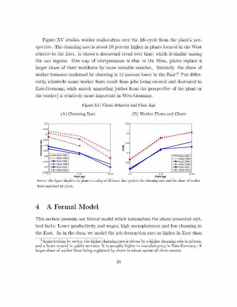
Figure XV studies worker reallocation over the life-cycle from the plant's per-

spective. The churning rate is about 10 percent higher in plants located in the West

relative to the East. It shows a downward trend over time, which is similar among

the two regions. One way of interpretation is that in the West, plants replace a

larger share of their workforce by more suitable matches. Similarly, the share of

worker turnover explained by churning is 12 percent lower in the East.9 Put dier-

ently, relatively many worker ows result from jobs being created and destroyed in

East-Germany, while match upgrading (either from the perspective of the plant or

the worker) is relatively more important in West-Germany.

Figure XV: Churn Behavior and Plant Age

(A) Churning Rate

1−3 4−19 20−390.065

0.07

0.075

0.08

0.085

0.09

0.095

0.1

0.105

0.11

Plant age

Ch

urn

ing

rat

e

East 1993West 1993East 1996West 1996East 2001West 2001

(B) Worker Flows and Churn

1−3 4−19 20−39

0.35

0.4

0.45

0.5

0.55

Plant age

CH

W

East 1993West 1993East 1996West 1996East 2001West 2001

Notes: The gure displays for plants entering at dierent time periods the churning rate and the share of worker

ows explained by churn.

4 A Formal Model

This section presents our formal model which rationalizes the above presented styl-

ized facts: Lower productivity and wages, high unemployment and low churning in

the East. As in the data, we model the job destruction rate as higher in East than

9Again looking by sector, the higher churning rate is driven by a higher churning rate in private,and a lesser extend in public services. It is actually higher in manufacturing in East-Germany. Alarger share of worker ows being explained by churn is robust across all three sectors.

20

in West-Germany. Put dierently, we do not adress the source of the dierence.

One could think of this as reecting plants in the East to miss the nancial means to

survive dicult times because household wealth is lower. Alternatively, it may result

from missing networks as in Uhlig (2006). The lower plant survival rate is consistent

with both of these stories. Our contribution is showing that we can rationalize a

substantial fraction of the productivity dierence between the two regions as a result

from changes in workers' search behavior that results from dierent job ow rates.

4.1 Model set-up

The economy is populated by a continuum of workers with mass one that are either

employed,et, or unemployed, ut. In both cases, workers can choose the probability λ

to nd an open vacancy. Exerting costs is costly for the worker but the costs may

depend on the employment status:

cE =f(λ)

cU =g(λ)

Both f and g are increasing and convex functions. Jobs have idiosyncratic productiv-

ity x, paying a wage w(x). Search is random and oers a drawn from a distribution

with CDF Γ(x) and nite support [x, x]. Reecting the common institutional setting,

we assume that this distribution is common in the two regions. The decision of the

unemployed worker reads:

U = maxλ

b− cU(λ) + β

[(1 − λ)U + λ

∫ x

x

V (x)dΓ(x)],

where b is the ow value of unemployment, β is the worker's discount factor, and

V (x) is the value of being employed at a plant with productivity x. We make the

implicit assumption that only job oers exist that are prefered to unemployment.

21

The value of employment reads:

V (x) = maxλ

w(x) − cE(λ)

+ β[(1 − δ(x,R))

((1 − λ)V (x) + λΩ(x)

)+ δ(x,R)U

],

where δ(x,R) is the job destruction rate which depends on plant productivity and

the region R and Ω(x) is the value of getting an outside job oer:

Ω(x) = λ(V (x)Γ(x) +

∫ y

y=x

V (y)dΓ(y)).

Because δ is higher in the East by assumption, the East also features a higher

unemployment rate. Consequently, these workers have less time to sort into highly

productive plants. Additional, on-the-job search is less attractive when job destruc-

tion is high. A high job destruction rate reduces the gains from being employed in a

high relative to a low productive plant. Therefore, workers perform less on-the-job

search in the East. As in the data, workers sort less into more productive plants and

the average plant productivity becomes even lower.

4.2 Calibration and Results (Incomplete)

Our calibration strategy is to match moments from job and worker ows in West-

Germany. Our target is the year 2000, where we stop to see convergence in job ow

rates conditional on the industry mix. We then ask how much of the productivity

dierence we can explain when imposing a job destruction rate that is, as in the

data, larger for each plant size.

We nd that average productivity is 10 percent lower in East than in West-

Germany. Put dierently, of the 30 percent productivity dierence, we can explain

1/3 by dierences in workers' search behavior resulting from higher job turnover in

East-Germany. In this sense, high job turnover rates seem not to be a driving force

of productivity growth in East-Germany after 1995 but rather a barrier to growth.

22

5 Conclusion

• Besides common legislation and institutions, labor productivity and wages are

30% lower in East than in West-Germany since 1994 and show no convergence.

• Neither missing convergence in capital intensity, labor force training, industry

composition, or a failure to allocate resources to the most productive growing

plants can explain these persistent dierences.

• Using a newly composed data-set, we show that job and worker ows are larger

in the East, a relatively high share of worker ows in the East result from jobs

being created and destroyed, and a relatively low share of workers work at high

productive plants in the East.

• We rationalize these facts using a model with endogenous on-the-job search.

23

A Structural Break Adjustment

This section describes how we perform structural break adjustment. Call any sea-

sonal adjusted series Y . For each Y we detect the number of structural breaks and

assign a dummy variable to each Dit that takes the value 1 during the break. We

have the following model for the DGP in mind:

Yt = β0 + β1D1t + ...+ βnDnt + ft + εt

where n is the number of structural breaks, εt is some short time uctuation and ft is

a smooth time trend that is estimated semi-parametrically. To be more specic, we

employ a local linear Gaussian kernel regression of the original series where points

in the structural break receive zero weight. We then compute the residual

Yt − ft = β0 + β1D1t + ...+ βnDnt

We regress this residual on the dened set of dummy variables to obtain their pre-

dicted eects βi. The structural break adjusted series is then computed by

Y sbt = Yt − β1D1t − ...− βnDnt

B Constructing Constant Industry Distributions

This section describes how we compute the time series for xed industry shares that

we use in Figure XII. Call the trend component (in levels) of a HP-ltered series

of industry j Xjt . Moreover, compute for each industry in each region its relative

dynamic employment share:

ecjt =emj

t

EMt

24

We now weight the current period series by initial relative employment shares:

X indt =

J∑j=1

(ecj1 ∗Xjt ),

where ecj1 is either the employment composition from East or West-Germany.

C Plant Entry

This section looks at the aspect of plants newly entering the market in East and

West-Germany. The top panel of Figure XVI looks at average plant entry in East

and West-Germany. The share of jobs created by new entering plants relative to

total employment was twice as high in East-Germany just after reunication, but it

falls throughout the sample converging to the level of West-Germany by 2006. The

average entrant was larger in East-Germany after reunication, but average size falls

throughout the sample in East-Germany, while it is increasing in West-Germany,

leading to larger entrants in West-Germany at the end of the sample.

Figure XVI: Entering Plants

(A) Entering Share of Employment

1994 1996 1998 2000 2002 2004 20064

5

6

7

8

9

10

11

12

13x 10

−3

Year

JC/E

MP

WestEast

(B) Average Size Entering

1994 1996 1998 2000 2002 2004 20063

3.5

4

4.5

Year

Ave

rag

e si

ze

WestEast

Notes: The gure shows the share of employment created by newly entering plants and the average size of entering

plants in East and West-Germany.

In the main text, we show that plant growth is very similar in East and West-

25

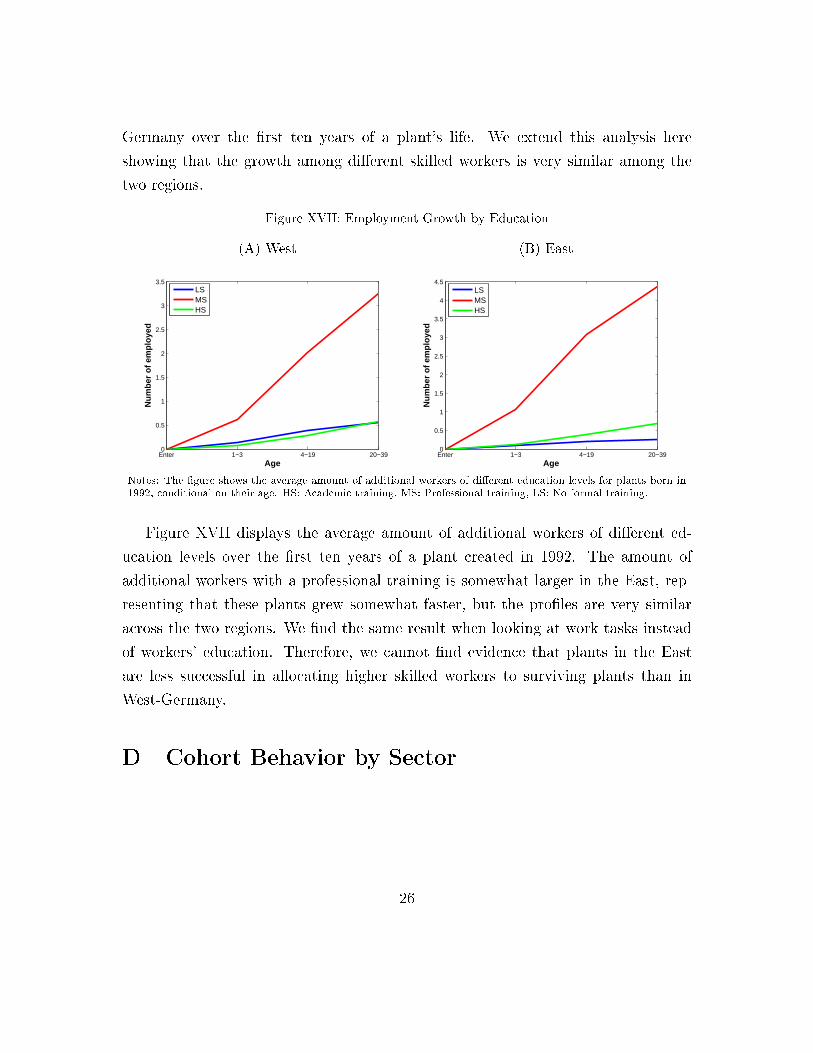
Germany over the rst ten years of a plant's life. We extend this analysis here

showing that the growth among dierent skilled workers is very similar among the

two regions.

Figure XVII: Employment Growth by Education

(A) West

Enter 1−3 4−19 20−390

0.5

1

1.5

2

2.5

3

3.5

Age

Nu

mb

er o

f em

plo

yed

LSMSHS

(B) East

Enter 1−3 4−19 20−390

0.5

1

1.5

2

2.5

3

3.5

4

4.5

Age

Nu

mb

er o

f em

plo

yed

LSMSHS

Notes: The gure shows the average amount of additional workers of dierent education levels for plants born in

1992, conditional on their age. HS: Academic training, MS: Professional training, LS: No formal training.

Figure XVII displays the average amount of additional workers of dierent ed-

ucation levels over the rst ten years of a plant created in 1992. The amount of

additional workers with a professional training is somewhat larger in the East, rep-

resenting that these plants grew somewhat faster, but the proles are very similar

across the two regions. We nd the same result when looking at work tasks instead

of workers' education. Therefore, we cannot nd evidence that plants in the East

are less successful in allocating higher skilled workers to surviving plants than in

West-Germany.

D Cohort Behavior by Sector

26

Figure XVIII: Survival Rates by Sector

(A) Manufacturing 1− 3

1993 1996 1998 2000 20010.84

0.85

0.86

0.87

0.88

0.89

0.9

0.91

0.92

% s

till i

n bu

sine

ss a

fetr

1−3

qua

rter

s

Year of existence

EastWest

(B) Manufacturing 4− 19

1997 2000 2002 2004 2005

0.5

0.55

0.6

0.65

% s

till i

n bu

sine

ss a

fetr

4−1

9 qu

arte

rs

Year of existence

EastWest

(C) Manufacturing 20− 39

2002 2005

0.26

0.28

0.3

0.32

0.34

0.36

0.38

0.4

0.42

0.44

0.46

% s

till i

n bu

sine

ss a

fetr

20−

39 q

uart

ers

Year of existence

EastWest

(D) PrivServ 1− 3

1993 1996 1998 2000 2001

0.76

0.78

0.8

0.82

0.84

0.86

% s

till i

n bu

sine

ss a

fetr

1−3

qua

rter

s

Year of existence

EastWest

(E) PrivServ 4− 19

1997 2000 2002 2004 2005

0.44

0.46

0.48

0.5

0.52

0.54

0.56

0.58

% s

till i

n bu

sine

ss a

fetr

4−1

9 qu

arte

rs

Year of existence

EastWest

(F) PrivServ 20− 39

2002 2005

0.28

0.3

0.32

0.34

0.36

0.38

% s

till i

n bu

sine

ss a

fetr

20−

39 q

uart

ers

Year of existence

EastWest

(G) PubServ 1− 3

1993 1996 1998 2000 2001

0.88

0.885

0.89

0.895

0.9

0.905

0.91

0.915

% s

till i

n bu

sine

ss a

fetr

1−3

qua

rter

s

Year of existence

EastWest

(H) PubServ 4− 19

1997 2000 2002 2004 2005

0.6

0.65

0.7

0.75

0.8

0.85

% s

till i

n bu

sine

ss a

fetr

4−1

9 qu

arte

rs

Year of existence

EastWest

(I) PubServ 20− 39

2002 2005

0.4

0.45

0.5

0.55

0.6

0.65

0.7

% s

till i

n bu

sine

ss a

fetr

20−

39 q

uart

ers

Year of existence

EastWest

Notes:

27

References

Boeri, T. and K. Terrell (2002): Institutional Determinants of Labor Reallo-

cation in Transition, Journal of Economic Perspectives, 16, 5176.

Burda, M. (2006): Factor Reallocation in Eastern Germany after Reunication,

American Economic Review (Papers and Proceedings), 96, 368374.

Davis, S. J., J. C. Haltiwanger, and S. Schuh (1996): Job Creation and

Destruction, MIT Press.

Foster, L., J. C. Haltiwanger, and C. Krizan (2001): Aggregate Produc-

tivity Growth, Lessons from Microeconomic Evidence, in New Developments in

Productivity Analysis, University of Chicago Press.

Fuchs-Schündeln, N. and R. Izem (2012): Explaining the Low Labor Produc-

tivity in East Germany - A Spatial Analysis, Journal of Comparative Economics,

40, 121.

Hall, R. E. and C. I. Jones (1999): Why do some Countries Produce so much

more Output per Worker than Other? Quarterly Journal of Economics, 114,

83116.

Haltiwanger, J. C., J. I. Lane, and J. R. Spletzer (1999): Productivity Dif-

ferences Across Employers: The Role of Employer Size, Age and Human Capital,

American Economic Review P&P, 89, 9498.

Hsieh, C.-T. and P. J. Klenow (2009): Misallocation and Manufacturing TFP

in China and India, Quarterly Journal of Economics, 124, 14031448.

(2012): The Life Cycle of Plants in India and Mexico, mimeo.

Restuccia, D. and R. Rogerson (2008): Policy Distortions and Aggregate

Productivity with Heterogeneous Plants, Review of Economic Dynamics, 11, 707

720.

28

Uhlig, H. (2006): Regional Labor Markets, Network Externalities and Migration:

The Case of German Reunication, American Economic Review (Papers and Pro-

ceedings), 96, 368374.

29