Labor Market Returns to an Early Childhood Stimulation

Labor Market Returns to an Early Childhood StimulationIntervention in Jamaica

Paul Gertler+,¶

James Heckman*,†,‡

Rodrigo Pinto*

Arianna Zanolini*

Christel Vermeerch§

Susan Walker]

Susan M. Chang]

Sally Grantham-McGregor[

April 25, 2014 3:30pm

A substantial literature shows that U.S. early childhood interventions have sig-nificant long-term economic benefits. There is little evidence on this questionfor developing countries. We report substantial effects on the earnings of par-ticipants in a randomized intervention conducted in 1986–1987 that gave psy-chosocial stimulation to growth-stunted Jamaican toddlers. The interventionconsisted of weekly visits from community health workers over a 2-year pe-riod that taught parenting skills and encouraged mothers and children to in-teract in ways that develop cognitive and socioemotional skills. The authorsre-interviewed 105 out of 129 study participants 20 years later and found thatthe intervention increased earnings by 25%, enough for them to catch up tothe earnings of a non-stunted comparison group identified at baseline (65 outof 84 participants).Key Words: early childhood development, stunting, randomized trialJEL Codes: 015, I20, I10, I25

Author Affiliations: +University of California Berkeley, ¶National Bureau of Economic Re-search (NBER), *University of Chicago, †American Bar Foundation, ‡Institute for Fiscal Stud-ies, University College London, §The World Bank, ]The University of The West Indies, [UniversityCollege LondonCorresponding Author Contact: [email protected]

1

1 Introduction

Early childhood, when brain plasticity and neurogenesis are very high, is an important period

for cognitive and psychosocial skill development (1–3). Investments and experiences during

this period create the foundations for lifetime success (4–13). A large body of evidence demon-

strates substantial positive impacts of early childhood development (ECD) interventions aimed

at skill development (14,15). ECD interventions are estimated to have substantially higher rates

of return than most remedial later-life skill investments. (6, 8, 13, 16).

More than 200 million children under the age of 5 currently living in developing countries

are at risk of not reaching their full developmental potential, with most living in extreme poverty

(17, 18). These children start disadvantaged, receive lower levels of parental investment, and

throughout their lives fall further behind the advantaged (15, 19, 20).

The evidence of substantial long-term economic benefits from ECD is primarily based on

U.S. data (21–30). There are reasons to suspect that these benefits may be higher in developing

countries. Children there typically live in homes where the environment is less stimulating

than in developed countries. As a result, they enter ECD programs with lower levels of skill.

Programs that boost skills are likely to have greater benefits in developing countries because

skills are less abundant there. For example, the returns to schooling are typically higher in

developing countries (31).

This paper reports estimates of the causal effects on earnings of an intervention that gave two

years of psychosocial stimulation to growth-stunted toddlers living in poverty in Jamaica (32).

To our knowledge, this is the first experimental evaluation of the impact of an ECD psychosocial

stimulation intervention on long-term economic outcomes in a developing country (33).

Unlike many other early childhood interventions with treatment effects that fade out over

time (8,13,15), the Jamaican intervention had large impacts on cognitive development 20 years

2

later (34). We show that the intervention had large positive effects on earnings, enough for

stunted participants to completely catch up with a non-stunted comparison group. The inter-

vention compensated for early developmental delays and reduced later-life inequality. The Ja-

maican intervention had substantially larger effects on earnings than any of the U.S. programs,

suggesting that ECD programs may be an effective strategy for improving long-term outcomes

of disadvantaged children in developing countries.

2 The Jamaican Study

The Jamaican Study enrolled 129 growth stunted children age 9–24 months that lived in Kingston,

Jamaica, in 1986–1987 (35). Section A of the Supplementary Online Materials (SOM) gives

a detailed description of the intervention and original study design. The children were strat-

ified by age and sex. Within each stratum, children were randomly assigned to one of four

groups: (1) psychosocial stimulation (N=32), (2) nutritional supplementation (N=32), (3) both

psychosocial stimulation and nutritional supplementation (N=32), and (4) a control group that

received neither intervention (N=33). The Jamaican study also surveyed a comparison group of

84 non-stunted children who lived nearby. All subjects were given access to free health care.

The stimulation intervention (groups 1 and 3) consisted of two years of weekly one-hour

play sessions at home with trained community health aides designed to develop child cognitive,

language and psychosocial skills. The stimulation arms of the Jamaica Study showed signif-

icant long-term cognitive benefits through age 22 (36, 37). Moreover, stimulation had posi-

tive impacts on psychosocial skills, schooling attainment and reduced participation in violent

crimes (36).

The nutritional intervention (groups 2 and 3) consisted of giving one kilogram of formula

containing 66% of daily-recommended energy (calories), protein and micronutrients provided

3

weekly for 24 months. The nutrition-only arm, however, had no long-term effect on any mea-

sured outcome (36, 38). In addition, there were no statistically significant differences in effects

between the stimulation and stimulation-nutrition arms on any long-term outcome although the

arm with both interventions had somewhat stronger outcomes (see SOM section D). Hence, we

combine the two psychosocial stimulation arms into a single “stimulation” treatment group and

combine the nutritional supplementation only group with the pure control group into a single

“control” group, understating the benefits of the joint intervention.

3 Methods

We resurveyed both the stunted and non-stunted samples in 2007-08, some 20 years after the

original intervention when the participants were approximately 22 years old. We found and in-

terviewed 105 out of the original 129 stunted study participants. This sample was balanced. We

only observe statistically significant differences in 3 out of 23 variables at baseline (SOM Ta-

ble S.1). In addition, there is no evidence of selective attrition. We also found and interviewed

65 out of the 84 children of the original comparison sample. For that sample there are signif-

icant differences in the baseline characteristics of the attrition and non-attrition groups (SOM

Table S.3).

We estimate the impact of the stimulation intervention on earnings by comparing the earn-

ings of the stunted-treatment group to those of the stunted-comparison group. In this paper,

we control for potential bias from baseline imbalances using Inverse Propensity Weighting

(IPW) (39). We then assess the degree to which the intervention enabled the stunted-treatment

group to catch up to the non-stunted comparison group by comparing the earnings of the treat-

ment group to those of the comparison group. In the catch-up analysis, we correct for potential

attrition bias using IPW weighting. See SOM section B for the analysis of baseline balance,

4

attrition, and the details of implementing IPW.

In order to better understand the external validity of our catch-up analysis, we compare the

non-stunted group to the general population using data on individuals 21-23 years old living in

the greater Kingston area from the 2008 Jamaican Labor Force Survey (JLF) survey. By age 22,

the non-stunted group attained comparable levels of skills as those of persons the same age who

were living in the Kingston Area interviewed in the JLF (SOM Table S.4). The two samples are

equally likely to still be in school and achieve the same educational level in terms of the highest

grade of schooling attained and passing national comprehensive matriculation exams.

Statistical inference is complicated by small sample size and multiple outcomes. We address

the problem of small sample size by using exact permutation tests as implemented in (21). We

correct for the danger of arbitrarily selecting statistically significant treatment effects in the

presence of multiple outcomes by performing multiple hypothesis testing based on the stepdown

algorithm proposed in (40). In addition, we aggregate over outcomes using a non-parametric

combining statistic. Section C of the SOM gives details.

4 Parental Investment and Migration

The stimulation intervention was designed to improve maternal-child interactions and the qual-

ity of parenting. Using the infant-toddler HOME score (41, 42), we examine whether treatment

resulted in more maternal investment in stimulation activities at home during the experimental

period. The HOME score captures the quality of parental interaction and investment in children

by observing the home environment and maternal activities with her child.

The intervention increased the HOME inventory during the intervention period. At baseline

there was no difference in parenting between treatment and control groups (SOM Table S.1). At

the end of the 2-year intervention the HOME inventory of the stunted treatment group was 16%,

5

greater than the that of the control group (p=0.01). However, the effect of the intervention on

home environment and maternal activities with her child appears to have declined afterwards.

Using a series of HOME-like questions designed to capture stimulation activities in mid-to-late

childhood (43), there was no difference between the treatment and control groups at 7 or later

at age 11.

While most of the direct parental stimulation encouraged by the intervention seems to have

occurred during the treatment period, the intervention may have also affected other types of

parental investments later in life that, in turn, also contributed to improved earnings. As chil-

dren exited the intervention period with higher skills, parents may have realized that invest-

ments, such as schooling, had higher returns than they might otherwise would have thought. In

fact, significant differences in schooling attainment appear at age 17 (36). By age 22, the treat-

ment group had 0.6 (p=.08) more years of schooling attainment than the control group. The

proportion of the treatment group still enrolled in full time school (0.22) was more than 5 times

larger than in the control group (0.04) (p <=.01).

The stimulation treatment may have improved children’s skills enough so that families were

encouraged to move overseas to take advantage of better education and labor market opportuni-

ties. The overall migration rate of the treatment group (0.22) was significantly higher than that

of the control group (0.12) (p-value = .09) implying that treatment is associated with migration.

5 Earnings

5.1 Measurement

We examine the impact of the stimulation intervention on average monthly earnings, which

are calcuated as total earnings through the date of the survey divided by the number of months

worked to that date. Earnings are expressed in 2005 dollars using the Jamaican CPI and are then

6

transformed into logs. Migrants’ earnings are first deflated to 2005 using the CPI of residence

and were then converted to Jamaican dollars using PPP adjusted exchange rates. In Section B.3

of SOM we report the results of all analyses separately for earnings from the first job, last job

and current job. See Section E of SOM for more details on the construction of these variables.

One issue is that in the treatment group there are more individuals who both work and attend

school full time than in the control group. Working, full-time students are likely to have lower

earnings than non-students with the same education. Hence, observed average earnings likely

understate the long run earnings of the treatment group more than the control group, implying

that we underestimate the long-run effects of treatment on earnings. We address this issue by

restricting the sample to earnings in full time jobs (at least 20 days per month), which excludes

those who had part-time jobs while primarily attending school. We additionally examine a

sample restricted to non-temporary permanent jobs (8 months a year or more) in order to omit

students working in summer jobs that may have been full time. Of the 105 individuals in the

sample, 103 had participated in the labor force, 99 had a full time job, and 75 had a non-

temporary full time job.

Another issue is the selective attrition of the migrants. We were able to locate and interview

14 out of the 23 migrants. Among those 14 migrants, we found a significantly larger share of

the treatment migrants than of the control migrants. Over-representation of treatment migrants

can be a source of bias as migrant workers earn substantially more than those who stay in

Jamaica. We address potential bias by imputing earnings for the 9 missing migrants. We replace

missing values with predicted log earnings from an OLS regression on treatment, gender and

migration status. Imputing the missing observations re-weights the data so that the treatment

and control groups of migrants are no longer under- or over-represented in the sample. In a

sensitivity analysis, we delete migrants and still find strong and statistically significant effects

of the program on earnings (see SOM section D.4).

7

5.2 Results

We begin by examining the impact of the intervention on densities of log earnings at age 22.

Panel A of Figure 1 presents Epanechnikov kernel density estimates of the treatment and control

groups estimated using bandwidths that minimize mean integrated squared error for Gaussian

data. The figures show that for all comparisons the densities of log earnings for the treatment

group are shifted everywhere to the right of the control group densities. The differences are

greater when we restrict the sample to full time workers and even greater when we restrict the

sample further to non-temporary workers.

The estimated impacts on log earnings, reported in Table 1, show that the intervention had

a large and statistically significant effect on earnings. Average earnings from full time jobs are

25% higher for the treatment group than for the control group, where the percent difference is

estimated by exp(β)− 1 and β denotes the treatment effect estimate from Table 1. The impact

is substantially larger for full-time permanent (non-temporary) jobs.

The results of the catch-up analysis, presented in Table 2, show that the stunted treatment

group caught up with the non-stunted comparison group, while the control group remained be-

hind. The differences in log-earnings between the non-stunted group and the stunted treatment

group are never statistically significant and average around zero. The graphs in Panel B in

Figure 1 generally show little difference between the earnings densities for the two groups. In

contrast, the stunted control group remains behind. The non-stunted comparison group consis-

tently earns significantly more than the stunted control group (Table 2).

SOM Section D presents the results of a range of specification tests that corroborate the

robustness of the estimates presented in Table 1. Specifically, we first examine treatment effects

separately for the pure stimulation intervention and for the combined stimulation/supplemental

intervention, and test whether we can pool the two arms Second, we test the hypothesis that

there is no effect of nutritional supplementation on log earnings and whether we can pool the

8

supplementation and pure control groups. Third, we examine the extent to which the estimates

may be affected by censoring that arises because we only observe the earnings of those em-

ployed who are in the labor force. Fourth, we examine the extent to which the imputation of the

earnings of missing migrants influences the estimates. Finally, we assess the extent to which

the IPW correction for baseline imbalance affected the estimates by re-estimating the effects of

treatment on earnings without the IPW weights.

6 Conclusions

This is the first study to experimentally evaluate the long-term impact of an early childhood

psychosocial stimulation intervention on earnings in a low income country. Twenty years af-

ter the intervention was conducted, we find that the earnings of the stimulation group are 25%

higher than those of the control group and caught up to the earnings of a non-stunted compar-

ison group. These findings show that a simple psychosocial stimulation intervention in early

childhood for disadvantaged children can have a substantial effect on labor market outcomes

and can compensate for developmental delays. The estimated impacts are substantially larger

than the impacts reported for the US–based interventions, suggesting that ECD interventions

may be an especially effective strategy for improving long-term outcomes of disadvantaged

children in developing countries.

9

References and Notes1. P. Huttenlocher, Brain research 163 (1979).

2. P. R. Huttenlocher, Neural plasticity: The effects of environment on the development of thecerebral cortex (Harvard University Press, Cambridge, MA, 2002).

3. R. A. Thompson, C. A. Nelson, American Psychologist 56, 5 (2001).

4. E. I. Knudsen, J. J. Heckman, J. Cameron, J. P. Shonkoff, Proceedings of the NationalAcademy of Sciences 103, 10155 (2006).

5. J. J. Heckman, Science 312, 1900 (2006).

6. J. J. Heckman, Economic Inquiry 46, 289 (2008).

7. P. Carneiro, J. J. Heckman, Inequality in America: What Role for Human Capital Policies?,J. J. Heckman, A. B. Krueger, B. M. Friedman, eds. (MIT Press, Cambridge, MA, 2003),pp. 77–239.

8. F. Cunha, J. J. Heckman, L. J. Lochner, D. V. Masterov, Handbook of the Economics ofEducation, E. A. Hanushek, F. Welch, eds. (North-Holland, Amsterdam, 2006), chap. 12,pp. 697–812.

9. G. J. van den Berg, M. Lindeboom, F. Portrait, American Economic Review 96, 290 (2006).

10. D. Almond, L. Edlund, H. Li, J. Zhang, Long-term effects of the 1959-1961 China famine:Mainland China and Hong Kong, Working Paper 13384, National Bureau of EconomicResearch (2007).

11. H. Bleakley, Quarterly Journal of Economics 122, 73 (2007).

12. S. L. Maccini, D. Yang, American Economic Review 99, 1006 (2009).

13. D. Almond, J. Currie, Handbook of Labor Economics, O. Ashenfelter, D. Card, eds. (Else-vier, North Holland, 2011), vol. 4B, chap. 15, pp. 1315–1486.

14. P. L. Engle, et al., The Lancet 369, 229 (2007).

15. P. L. Engle, et al., The Lancet 378, 1339 (2011).

16. J. J. Heckman, Research in Economics 54, 3 (2000).

17. S. Grantham-McGregor, et al., The Lancet 369, 60 (2007).

18. S. P. Walker, et al., The Lancet 369, 145 (2007).

10

19. C. Paxson, N. Schady, Journal of Human Resources 42, 49 (2007).

20. L. Fernald, P. Kariger, M. Hidrobo, P. Gertler, Proceedings of the National Academy ofSciences (Supplement 2) 109, 17273 (2012).

21. J. J. Heckman, S. H. Moon, R. Pinto, P. A. Savelyev, A. Q. Yavitz, Quantitative Economics1, 1 (2010).

22. J. J. Heckman, S. H. Moon, R. Pinto, P. A. Savelyev, A. Q. Yavitz, Journal of PublicEconomics 94, 114 (2010).

23. A. J. Reynolds, S.-R. Ou, J. W. Topitzes, Child Development 75, 1299 (2004).

24. A. J. Reynolds, et al., Archives of Pediatrics and Adolescent Medicine 161, 730 (2007).

25. A. J. Reynolds, J. A. Temple, S.-R. Ou, I. A. Arteaga, B. A. B. White, Science 333, 360(2011).

26. F. A. Campbell, C. T. Ramey, E. Pungello, J. Sparling, S. Miller-Johnson, Applied Devel-opmental Science 6, 42 (2002).

27. F. A. Campbell, et al., Developmental Psychology 48, 1033 (2012).

28. F. Campbell, et al. (2013). Under review, Science.

29. A. Aughinbaugh, Journal of Human Resources 36, 641 (2001).

30. E. Garces, D. Thomas, J. Currie, American Economic Review 92, 999 (2002).

31. G. Psacharopoulos, H. A. Patrinos, Education Economics 12, 1469 (2004).

32. S. M. Grantham-McGregor, C. A. Powell, S. P. Walker, J. H. Himes, The Lancet 338, 1(1991).

33. There are, however, experimental studies that show that early life nutritional interventionsalso have substantial impacts on earnings (44).

34. S. P. Walker, S. M. Chang, M. Vera-Hernandez, S. Grantham-McGregor, Pediatrics 127,849 (2011).

35. S. Walker, C. Powell, S. Grantham-McGregor, European Journal of Clinical Nutrition 44,527 (1990).

36. S. P. Walker, S. M. Chang, C. A. Powell, S. M. Grantham-McGregor, The Lancet 366, 1804(2005).

11

37. S. P. Walker, S. M. Chang, M. Vera-Hernandez, S. Grantham-McGregor, Pediatrics 127,849 (2011).

38. S. P. Walker, S. M. Grantham-McGregor, C. A. Powell, S. M. Chang, Journal of Pediatrics137, 36 (2000).

39. J. M. Robins, A. Rotnitzky, L. P. Zhao, Journal of the American Statistical Association 89,846 (1994).

40. J. P. Romano, M. Wolf, Journal of the American Statistical Association 100, 94 (2005).

41. B. M. Caldwell, Pediatrics 40, 46 (1967).

42. B. M. Caldwell, R. H. Bradley, HOME observation for measurement of the environment(University of Arkansas at Little Rock, Little Rock, AR, 1984).

43. S. Grantham-McGregor, S. Walker, S. Chang, C. Powell, American Journal of ClinicalNutrition 66, 247 (1997).

44. J. Hoddinott, J. A. Maluccio, J. R. Behrman, R. Flores, R. Martorell, The Lancet 371, 411(2008).

45. P. V. Hamill, et al., The American Journal of Clinical Nutrition 32, 607 (1979).

46. I. C. Uzgiris, J. M. Hunt, Assessment in infancy: Ordinal scales of psychological develop-ment. (University of Illinois Press., Urbana, IL, 1975).

47. S. Walker, S. Grantham-McGregor, C. Powell, J. Himes, D. Simeon, American Journal ofClinical Nutrition 56, 504 (1992).

48. S. P. Walker, C. A. Powell, S. M. Grantham-McGregor, J. H. Himes, S. M. Chang, AmericanJournal of Clinical Nutrition 54, 642 (1991).

49. J. A. Maluccio, et al., Economic Journal 119, 734 (2009).

50. J. P. Romano, M. Wolf, Econometrica 73, 1237 (2005).

Acknowledgements: Acknowledgements: The authors gratefully acknowledge research support from the WorldBank Strategic Impact Evaluation Fund, the American Bar Foundation, The Pritzker Children’s Initiative, NICHDR37HD065072, R01HD54702, the Human Capital and Economic Opportunity Global Working Group - an initia-tive of the Becker Friedman Institute for Research in Economics funded by the Institute for New Economic Think-ing (INET), a European Research Council grant hosted by University College Dublin, DEVHEALTH 269874, andan anonymous funder. We have benefitted from comments of participants in seminars at the University of Chicago,UC Berkeley, MIT, the 2011 LACEA Meetings in Santiago Chile and the 2013 AEA Meetings. We thank thestudy participants for their continued cooperation and willingness to participate, and to Sydonnie Pellington forconducting the interviews. The authors have not received any compensation for the research nor do they have anyfinancial stake in the analyses reported here. Replication data for this article has been deposited at ICPSR and canbe accessed here: http://doi.org/10.3886/E2402V1.

12

http://doi.org/10.3886/E2402V1

Tables and Figures

13

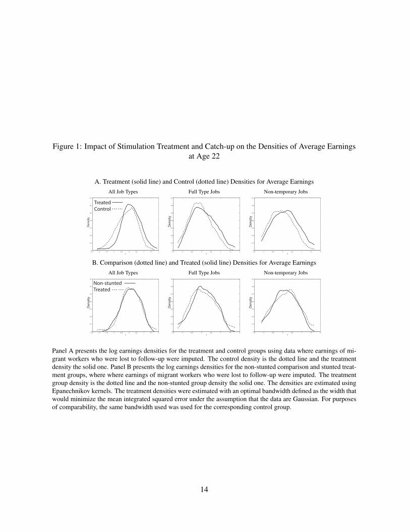
Figure 1: Impact of Stimulation Treatment and Catch-up on the Densities of Average Earningsat Age 22

A. Treatment (solid line) and Control (dotted line) Densities for Average EarningsAll Job Types Full Type Jobs Non-temporary Jobs

−2.5 −2 −1.5 −1 −0.5 0 0.5 1 1.5 20

0.1

0.2

0.3

0.4

0.5

0.6

0.7

Den

sity

x

TreatedControl

−1.5 −1 −0.5 0 0.5 1 1.5 20

0.1

0.2

0.3

0.4

0.5

0.6

0.7

Den

sity

x−1.5 −1 −0.5 0 0.5 1 1.5 20

0.1

0.2

0.3

0.4

0.5

0.6

0.7

Den

sity

x

B. Comparison (dotted line) and Treated (solid line) Densities for Average EarningsAll Job Types Full Type Jobs Non-temporary Jobs

−2.5 −2 −1.5 −1 −0.5 0 0.5 1 1.5 20

0.1

0.2

0.3

0.4

0.5

0.6

0.7

Den

sity

x

Non-stuntedTreated

−1.5 −1 −0.5 0 0.5 1 1.5 20

0.1

0.2

0.3

0.4

0.5

0.6

0.7

Den

sity

x−1.5 −1 −0.5 0 0.5 1 1.5 20

0.1

0.2

0.3

0.4

0.5

0.6

0.7

Den

sity

x

Panel A presents the log earnings densities for the treatment and control groups using data where earnings of mi-grant workers who were lost to follow-up were imputed. The control density is the dotted line and the treatmentdensity the solid one. Panel B presents the log earnings densities for the non-stunted comparison and stunted treat-ment groups, where where earnings of migrant workers who were lost to follow-up were imputed. The treatmentgroup density is the dotted line and the non-stunted group density the solid one. The densities are estimated usingEpanechnikov kernels. The treatment densities were estimated with an optimal bandwidth defined as the width thatwould minimize the mean integrated squared error under the assumption that the data are Gaussian. For purposesof comparability, the same bandwidth used was used for the corresponding control group.

14

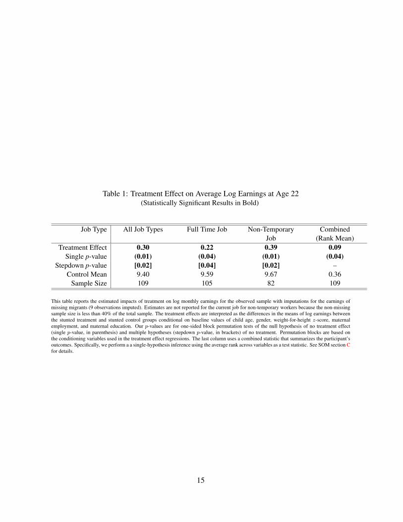
Table 1: Treatment Effect on Average Log Earnings at Age 22(Statistically Significant Results in Bold)

Job Type All Job Types Full Time Job Non-Temporary CombinedJob (Rank Mean)

Treatment Effect 0.30 0.22 0.39 0.09Single p-value (0.01) (0.04) (0.01) (0.04)

Stepdown p-value [0.02] [0.04] [0.02] –Control Mean 9.40 9.59 9.67 0.36

Sample Size 109 105 82 109

This table reports the estimated impacts of treatment on log monthly earnings for the observed sample with imputations for the earnings ofmissing migrants (9 observations imputed). Estimates are not reported for the current job for non-temporary workers because the non-missingsample size is less than 40% of the total sample. The treatment effects are interpreted as the differences in the means of log earnings betweenthe stunted treatment and stunted control groups conditional on baseline values of child age, gender, weight-for-height z-score, maternalemployment, and maternal education. Our p-values are for one-sided block permutation tests of the null hypothesis of no treatment effect(single p-value, in parenthesis) and multiple hypotheses (stepdown p-value, in brackets) of no treatment. Permutation blocks are based onthe conditioning variables used in the treatment effect regressions. The last column uses a combined statistic that summarizes the participant’soutcomes. Specifically, we perform a a single-hypothesis inference using the average rank across variables as a test statistic. See SOM section Cfor details.

15

Table 2: Catch Up - Comparison of Average Earning at Age 22 of the non-stunted and stuntedtreatment and control samples

(Statistically Significant Results in Bold)

Panel (I) Non-stunted - treatment

Job Type All Job Full Time Non-Temporary Combined

Types Job Job (Rank Mean)

Treatment Effect -0.06 -0.08 -0.24 -0.01Single p-value (0.68) (0.75) (0.94) (0.59)


Sample Size 120 116 97 120

Panel (II) Non-stunted - control

Job Type All Job Full Time Non-Temporary Combined

Types Job Job (Rank Mean)



Sample Size 121 119 101 121

The table presents estimates of the difference in the means of log earnings between respectively (I) the weightednon-stunted comparison group and the stunted cognitive stimulation group and (II) the weighted non-stunted com-parison group and the stunted control group. Our p-values are for one-sided block permutation tests of the nullhypothesis of complete catch up on each outcome (single p-value, in parentheses) and accounting for multiplehypotheses (stepdown p-values, in brackets). Permutation blocks are based on gender only, but do not controlfor differences in baseline values because the aim is to test for catch-up despite the initial disadvantage. The lastcolumn uses a combined statistic that summarizes the participant’s outcomes. Specifically, we perform a a single-hypothesis inference using the average rank across variables as a test statistic. See SOM section C for details.

16

Supplementary Online Materials

1

Contents

A The Jamaican Study 3

A.1 Intervention and Experimental Design . . . . . . . . . . . . . . . . . . . . . . . . . . . . . . . . 3

A.2 External Comparison Group . . . . . . . . . . . . . . . . . . . . . . . . . . . . . . . . . . . . . 4

A.3 Previous Studies . . . . . . . . . . . . . . . . . . . . . . . . . . . . . . . . . . . . . . . . . . . . 4

B The New Survey 6

B.1 Stunted Experimental Sample . . . . . . . . . . . . . . . . . . . . . . . . . . . . . . . . . . . . . 6

B.2 Non-Stunted Comparison Sample . . . . . . . . . . . . . . . . . . . . . . . . . . . . . . . . . . 7

B.3 Baseline, Attrition, External Validity and Treatment Effect Tables . . . . . . . . . . . . . . . . . 8

C Methodology 18

D Robustness Tests 20

D.1 Empirical Analysis . . . . . . . . . . . . . . . . . . . . . . . . . . . . . . . . . . . . . . . . . . 21

D.2 Pooling of Stimulation/Supplementation arms . . . . . . . . . . . . . . . . . . . . . . . . . . . . 21

D.3 The Effect of Nutritional Supplementation on Log-earnings . . . . . . . . . . . . . . . . . . . . . 22

D.4 Adjustments for Migration and Baseline Imbalance . . . . . . . . . . . . . . . . . . . . . . . . . 23

D.5 Catchup and Migrants . . . . . . . . . . . . . . . . . . . . . . . . . . . . . . . . . . . . . . . . . 23

D.6 Gender Comparison . . . . . . . . . . . . . . . . . . . . . . . . . . . . . . . . . . . . . . . . . . 23

E Construction of Earnings Variables 34

2

A The Jamaican Study

A.1 Intervention and Experimental Design

In 1986-1987, the Jamaican Study enrolled 129 stunted children age 9-24 months that lived in poor disadvantaged

neighborhoods of Kingston, Jamaica (35). Enrollment was conditioned on stunting because it is an easily and

accurately observed indicator of malnutrition that is strongly associated with poor cognitive development (18).

Stunting was defined using international standards as having a height less than two standard deviations of reference

data by age and sex (45). The children were stratified by age (above and below 16 months) and sex. Within each

stratum, children were sequentially assigned to one of four groups by random assignment. The four groups were

(1) psychosocial stimulation (N=32), (2) nutritional supplementation (N=32), (3) both psychosocial stimulation

and nutritional supplementation (N=32), and (4) a control group that received neither intervention (N=33). All

children were given access to free health care regardless of the group to which they were assigned.

The stimulation intervention (comprising groups 1 and 3) consisted of two years of weekly one-hour play

sessions at home with trained community health aides1 designed to develop child cognitive, language and psy-

chosocial skills. Activities included mediating the environment through labeling, describing objects and actions in

the environment, responding to the child’s vocalizations and actions, playing educational games, and using picture

books and songs that facilitated language acquisition. The first 18 months included Pigetian concepts such as use of

a tool and object permanence (46). After 18 months concepts such as size, shape, quantity, color and classification

based on Palmer (1971) were included. Particular emphasis was placed on the use of praise and giving positive

feedback to both the mother and child. Each session’s curriculum was adjusted to the child so that activities were

at the appropriate level for the child.

A major focus of the weekly visits was on improving the quality of the interaction between mother and child.

At every visit the use of homemade toys was demonstrated and the toys were left for the mother and child to use

until the next visit when they were replaced with different ones. Mothers were encouraged to continue the activities

between visits. The intervention was innovative not only for its focus on structured activities to promote cognitive,

language and socio-emotional development but also for its emphasis on supporting the mothers to promote their

child’s development.

1The aides had completed at least secondary education and training in nutrition and primary heatlh care as partof the government job. They were seconded to the study and received an additional 8 weeks of training in childdevelopment, teaching techniques and toy making (35).

3

The nutritional intervention (comprising groups 2 and 3) was aimed at compensating for the nutritional de-

ficiencies that may have caused stunting. The nutritional supplements, provided weekly for 18 months, con-

sisted of one kilogram of formula containing 66% of daily-recommended energy (calories), and 100% of daily-

recommended protein and micronutrients (see (47) for details). In addition, in an attempt to minimize sharing of

the formula with other family members, the family also received 0.9 kilograms of cornmeal and skimmed milk

powder. Despite this, sharing was common and uptake of the supplement decreased significantly during the inter-

vention (48).

Of the 129 study participants, two of the participants dropped out before completion of the two-year program.

The remaining 127 participants were surveyed at baseline, resurveyed immediately following the the end of the

two-year intervention, and again at ages 7, 11, and 17. Our analysis is based on a re-interview of the sample in

2007-08 when the participants were approximately 22 years old, some 20 years after the original intervention. We

obtained 105 interviews at age 22.

A.2 External Comparison Group

For comparison purposes, the study also enrolled a sample of non-stunted children from the same neighborhoods,

where non-stunted was defined as having a height for age z-score greater than -1 standard deviations. At baseline,

every fourth stunted child in the study was matched with one non-stunted child who lived nearby and was the same

age (plus or minus 3 months) and sex. At age 7, this sample of 32 was supplemented with another 52 children who

had been identified in the initial survey as being non-stunted and fulfilled all other inclusion criteria. Members of

the non-stunted comparison group did not receive any intervention, but did receive the same free health care as

those in the stunted experimental group. From age 7 onwards, this group was surveyed at the same time as the

participants in the experiment.

A.3 Previous Studies

The stimulation and the combined stimulation-nutrition arms of the Jamaica Study proved to have a large long-term

impact on cognitive development. At the end of the 2-year intervention, the developmental levels of children who

received stimulation were significantly above the control group and approached those of the external non-stunted

group (32). While cognitive benefits decreased somewhat by age 7, significant long-term benefits were sustained

through age 22 (36, 37). Moreover, stimulation had positive impacts on psychosocial skills, schooling attainment

4

and reduced participation in violent crimes (36).

While the stimulation arms had strong and lasting effects, the nutrition-only arm had no long-term effect

on any measured outcome (36, 38).2 In addition, there were no statistically significant or quantitatively important

differences in effects between the stimulation and stimulation-nutrition arms on any long-term outcome. Hence, we

combine the two psychosocial stimulation arms into a single treatment group (N=64) and combine the nutritional

supplementation only group with the pure control group into a single control group (N=65).3 Henceforth we use

the term stimulation effects of stunted participants to designate the analysis that compares groups 1 and 3 against

groups 2 and 4.

2This is in contrast to the Guatemala Study in which nutritional supplementation did affect both long-termhealth status and earnings ( (44); (49)). Supplementation in Jamaica may have begun too late to have had animpact. The Guatemala study started supplementing children in utero and at birth, before the children becamemalnourished, while the Jamaican program started at later ages after the children were already malnourished. Otherpossible reasons for the difference include the fact that the supplement was more intensively shared with otherfamily members in Jamaica and the supplement was a smaller share of the total food budget in Jamaica (35,44,47).

3We formally test the hypotheses that groups 1 and 3 and be pooled, that groups 2 and 4 can pooled, and thatsupplementation had no impact on earnings in Appendix D.2.

5

B The New Survey

We resurveyed both stunted (experimental) and non-stunted (comparison) study populations in 2007-08 some 20

years after the original intervention when the participants were approximately 22 years old.4 We attempted to find

all of the study participants regardless of current location and followed migrants to the the US, Canada, and the

UK. When we could not find a participant in Jamaica, we contacted relatives for further information to find the

participants.

B.1 Stunted Experimental Sample

We were able to find and interview 105 out of the original 127 (83%) stunted participants who completed the

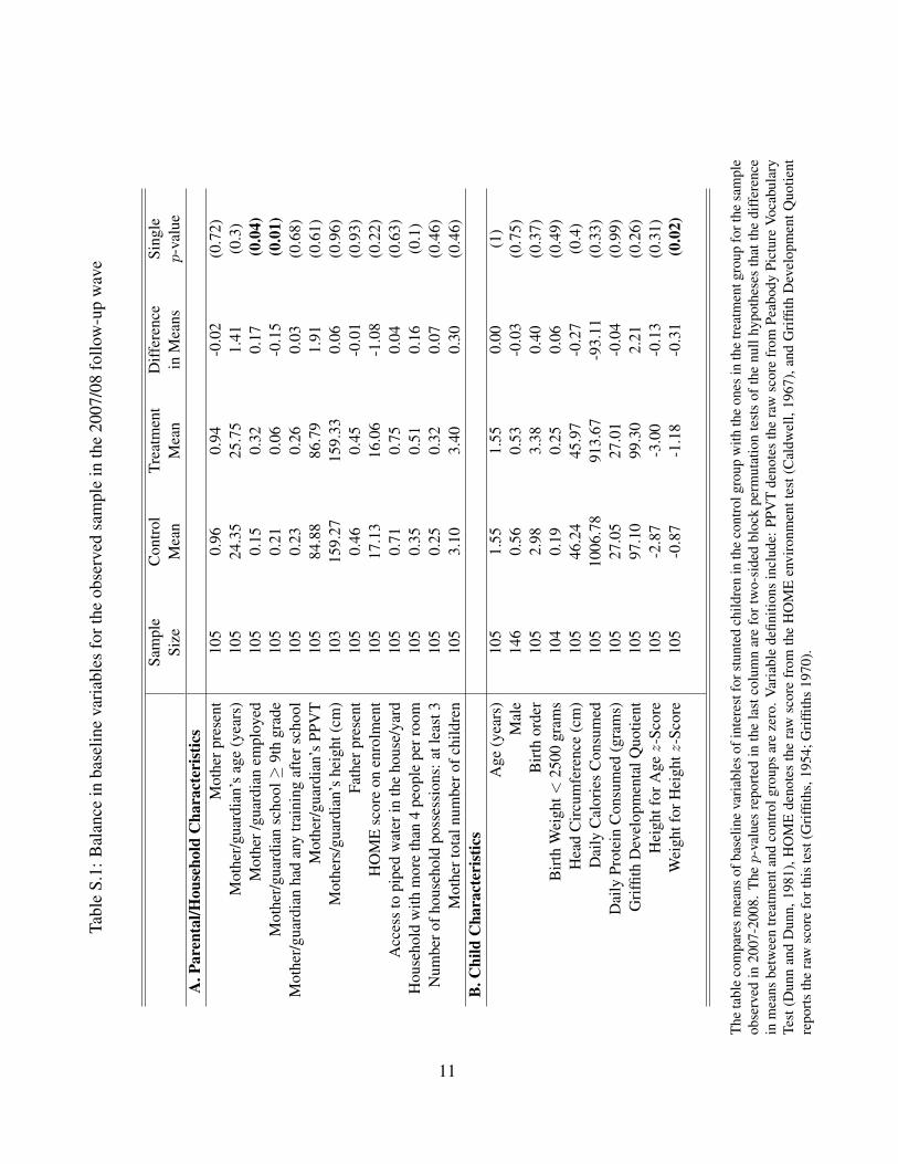
program. The stunted sample remained balanced as we only observe significant differences in 3 out of 23 variables

(Table S.1). Mothers of children in the treatment group were more likely to be employed and have completed less

schooling than mothers of children in the control group, and children in the treatment group had lower weight for

height than children in the control group. These imbalances are already present in the full baseline sample of 127,

which suggests that they were the result of sampling variation in the original randomization rather than differential

sample attrition. We control for baseline imbalances using Inverse Propensity Weighting (IPW), which re-weights

observed data using predicted probabilities of treatment (39). The predictions come from a logit model of treatment

assignment as a function of the baseline characteristics whose means are significantly different between treatment

and control groups.

Twenty-two (17%) of the 127 original participants were not interviewed, of which 10 were not found, 9

died, and 3 of those who were found refused to be interviewed. Of the 13 that were not found or refused to be

interviewed, 9 were migrants. Treatment status is not a significant predictor of the overall probability of attrition

and the baseline means of none of the 23 individual variables are not significantly different between the group

that dropped out and the group that stayed in the sample, even when we stratify by treatment and control (Table

S.2). Hence, in terms of measured variables, there appears to be no selective attrition and the remaining sample is

representative of the original sample.

We examine the impact of the intervention on densities of log earnings. Figure S.1 presents Epanechnikov

kernel density estimates of the treatment and control groups estimated using bandwidths that minimize mean

integrated squared error for Gaussian data. The Figure shows the estimated density for the earnings variables

4The survey received ethical clearance from the IRB of the University of the West Indies in Kingston, Jamaica.

6

associated with first, last and current job.

B.2 Non-Stunted Comparison Sample

We found and interviewed 65 children out of the 84 children originally surveyed with an implied attrition rate of

23%, which is slightly higher than that for the experimental sample. There are, however, significant differences

in the baseline characteristics of the attrition and non-attrition groups for 4 out of the 15 variables in the non-

stunted sample (SOM Table S.3). Mothers in the attrition group are older, perform better on the Picture Peabody

Verbal Test (PPVT), provide more verbal stimulation to their children and live in better houses than mothers who

do not attrit. We correct for attrition using IPW to re-weight the observed data using predicted probabilities of

attrition (39). The predictions come from a logit model of attrition as a function of the baseline characteristics

whose means are statistically significantly different between attrited and non-attrited groups.

In order to better understand the external validity of our catch-up analysis we compare the non-stunted group

to the general population using data on individuals 21-23 years old living in the greater Kingston area from the

2008 Jamaica Labor Force (JLF) survey that was collected in the same year as the last follow-up. Unfortunately,

the labor supply and earnings questions in the JLF and in our survey were asked in different ways, and there was a

50% non-response rate in the JLF to the earnings questions among those who were employed. Only the education

variables are directly comparable. By age 22, the non-stunted group attained comparable levels of human capital

as those of the same age and living in the Kingston Area interviewed in the Labor Force Survey (SOM Table S.4).

The two samples are equally likely to still be in school and achieve the same level of educational attainment in

terms of years of schooling and passing national comprehensive matriculation exams. This suggests that the human

capital of the non-stunted comparison group is not different from a representative sample of youth in the Kingston

area during the study period.

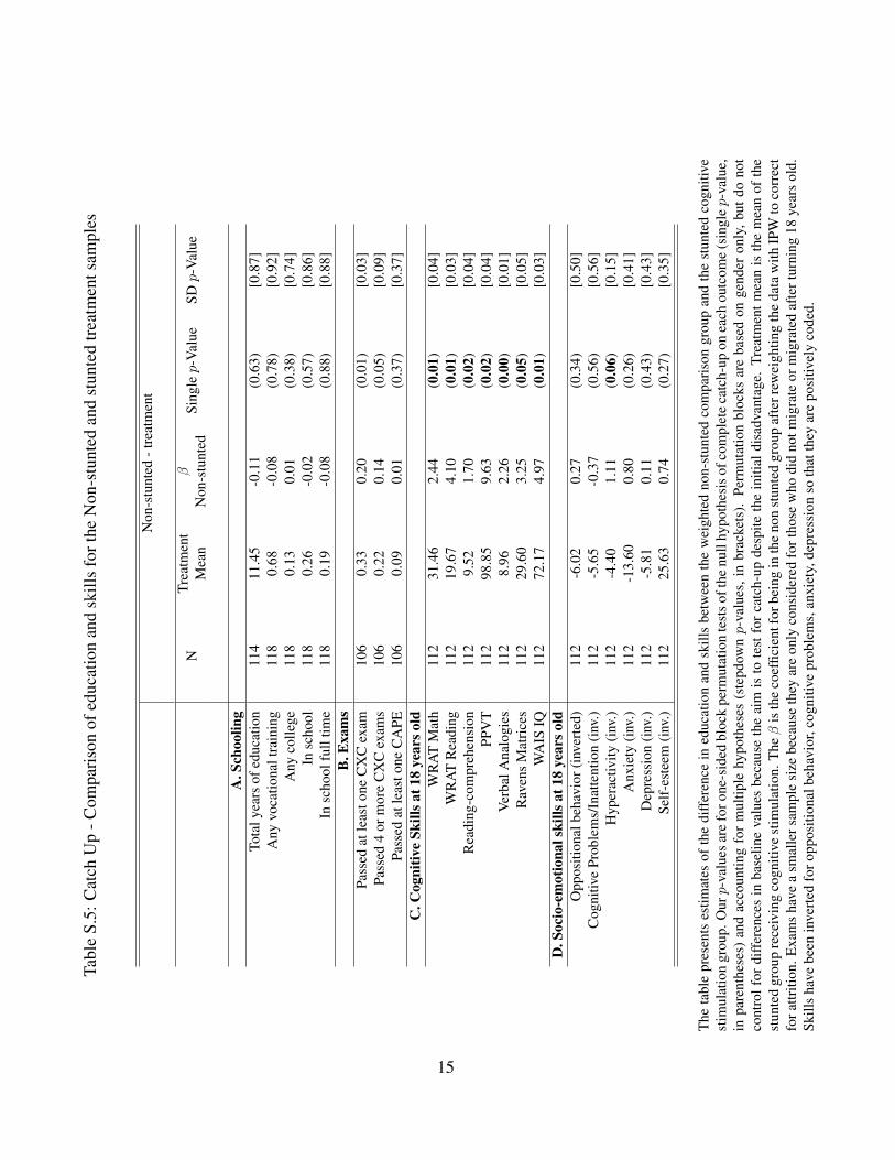
Table S.5 compares education at 22 years old and skills at 18 years old for the non-stunted comparison sample

and the stunted sample in the treatment group. The non-stunted comparison sample performs consistently better

only in measurements for cognitive skills, but cannot be distinguished from the stunted treated group for all other

dimensions.

Figure S.2 presents the Kernel estimates of the earnings densities for the comparison and treatment group. The

Figure shows the estimated density for the earnings variables associated with first, last and current job. The next

section presents an empirical analysis of baseline variables, attrition and external validity.

7

B.3 Baseline, Attrition, External Validity and Treatment Effect Tables

This Appendix presents descriptive statistics of baseline variables as well as tests for baseline of the treatment and

control stunted sample, selective attrition and external validity.

Table S.1 investigates whether baseline means of the stunted sample are balanced between treatment and

control groups. The table reports means of the two groups and the difference in means. The p-values are for

two-sided permutation tests of the null hypotheses that the baseline means of the treatment and control groups are

equal. We only observe statistically significant differences in 3 out of the 23 variables we examined.

Table S.2 investigates if there is evidence for non-random attrition in the stunted sample. The p-values are for

two-sided permutation tests of the null hypotheses that the baseline means of the sample found in the 2008 and

the sample not found in 2008 are equal. The first column of the table reports p-values for the full sample and the

next two columns report the p-values separately for, respectively, the treatment and control samples. We found no

statistically significant differences between the missing and non-missing samples.

Table S.3 investigates if there is evidence for non-random attrition in the non-stunted comparison sample. The

p-values for two-sided permutation tests of the null hypotheses that the baseline descriptive statistics for the non-

stunted sample found in the 2008 survey (Non-Attrited) and the group lost in the 2008 survey (Attrited) are equal.

We observe statistically significant differences in 4 out of the 15 variables we examined.

Table S.4 examines the external validity of non-stunted comparison group. It compares human capital mea-

sures from the non-stunted sample collected in 2008 with individuals age 22 and 23 years old living in Kingston

Metropolitan Area from from the 2008 Jamaica Labor Force (JLF) survey. The p-values are for for two-sided

permutation tests of the null hypotheses that the difference in means between the Jamaican non-stunted sample

and the JLF sample is zero.

Table S.6 reports the estimated impacts of treatment on log monthly earnings for the observed sample with

imputations for the earnings of missing migrants (9 observations imputed). It displays the analysis of three types

of earnings associated with the available data on the participant first job, last job and current job.

Table S.7 examines the catch up effect on Log Earnings between the non-stunted and stunted treatment and

control samples. It displays the type of variables examined in Table S.6. Namely, earnings associated with the

available data on the participant first job, last job and current job.

8

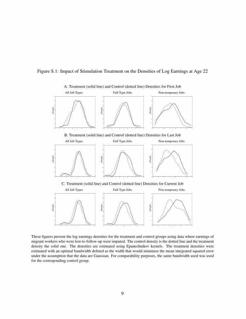
Figure S.1: Impact of Stimulation Treatment on the Densities of Log Earnings at Age 22

A. Treatment (solid line) and Control (dotted line) Densities for First JobAll Job Types Full Type Jobs Non-temporary Jobs

−2.5 −2 −1.5 −1 −0.5 0 0.5 1 1.5 20

0.1

0.2

0.3

0.4

0.5

0.6

0.7

Den

sity

x−2.5 −2 −1.5 −1 −0.5 0 0.5 1 1.5 2 2.50

0.1

0.2

0.3

0.4

0.5

0.6

0.7

Den

sity

x−1.5 −1 −0.5 0 0.5 1 1.5 20

0.1

0.2

0.3

0.4

0.5

0.6

0.7

Den

sity

x

B. Treatment (solid line) and Control (dotted line) Densities for Last JobAll Job Types Full Type Jobs Non-temporary Jobs

−4 −3 −2 −1 0 1 2 30

0.1

0.2

0.3

0.4

0.5

0.6

0.7

Den

sity

x−2.5 −2 −1.5 −1 −0.5 0 0.5 1 1.5 2 2.50

0.1

0.2

0.3

0.4

0.5

0.6

0.7

Den

sity

x−1.5 −1 −0.5 0 0.5 1 1.5 20

0.1

0.2

0.3

0.4

0.5

0.6

0.7

Den

sity

x

C. Treatment (solid line) and Control (dotted line) Densities for Current JobAll Job Types Full Type Jobs Non-temporary Jobs

−4 −3 −2 −1 0 1 2 30

0.1

0.2

0.3

0.4

0.5

0.6

0.7

Den

sity

x−3 −2 −1 0 1 2 30

0.1

0.2

0.3

0.4

0.5

0.6

0.7

Den

sity

x−2 −1.5 −1 −0.5 0 0.5 1 1.50

0.1

0.2

0.3

0.4

0.5

0.6

0.7

Den

sity

x

These figures present the log earnings densities for the treatment and control groups using data where earnings ofmigrant workers who were lost-to-follow-up were imputed. The control density is the dotted line and the treatmentdensity the solid one. The densities are estimated using Epanechnikov kernels. The treatment densities wereestimated with an optimal bandwidth defined as the width that would minimize the mean integrated squared errorunder the assumption that the data are Gaussian. For comparability purposes, the same bandwidth used was usedfor the corresponding control group.

9

Figure S.2: Catch up of Treatment Group Earnings to Comparison Group Earnings at Age 22

A. Comparison (dotted line) and Treated (solid line) Densities for First JobAll Job Types Full Type Jobs Non-temporary Jobs

−2.5 −2 −1.5 −1 −0.5 0 0.5 1 1.5 20

0.1

0.2

0.3

0.4

0.5

0.6

0.7

Den

sity

x−2.5 −2 −1.5 −1 −0.5 0 0.5 1 1.5 2 2.50

0.1

0.2

0.3

0.4

0.5

0.6

0.7

Den

sity

x−1.5 −1 −0.5 0 0.5 1 1.5 20

0.1

0.2

0.3

0.4

0.5

0.6

0.7

Den

sity

x

B. Comparison (dotted line) and Treated (solid line) Densities for Last JobAll Job Types Full Type Jobs Non-temporary Jobs

−4 −3 −2 −1 0 1 2 30

0.1

0.2

0.3

0.4

0.5

0.6

0.7

Den

sity

x−2.5 −2 −1.5 −1 −0.5 0 0.5 1 1.5 2 2.50

0.1

0.2

0.3

0.4

0.5

0.6

0.7

Den

sity

x−1.5 −1 −0.5 0 0.5 1 1.5 20

0.1

0.2

0.3

0.4

0.5

0.6

0.7

Den

sity

x

C. Comparison (dotted line) and Treated (solid line) Densities for Current JobAll Job Types Full Type Jobs Non-temporary Jobs

−4 −3 −2 −1 0 1 2 30

0.1

0.2

0.3

0.4

0.5

0.6

0.7

Den

sity

x−3 −2 −1 0 1 2 30

0.1

0.2

0.3

0.4

0.5

0.6

0.7

Den

sity

x−2 −1.5 −1 −0.5 0 0.5 1 1.50

0.1

0.2

0.3

0.4

0.5

0.6

0.7

Den

sity

x

These figures present the log earnings densities for the non-stunted comparison and stunted treatment Groups,where where earnings of migrant workers who were lost to follow-up were imputed. The treatment group densityis the dotted line and the non-stunted group density the solid one. The densities are estimated using Epanech-nikov kernels. The treatment densities were estimated with an optimal bandwidth defined as the width that wouldminimize the mean integrated squared error under the assumption that the data are Gaussian. For comparabilitypurposes, the same bandwidth used was used for the corresponding control group.

10

Tabl

eS.

1:B

alan

cein

base

line

vari

able

sfo

rthe

obse

rved

sam

ple

inth

e20

07/0

8fo

llow

-up

wav

e

Sam

ple

Con

trol

Trea

tmen

tD

iffer

ence

Sing

leSi

zeM

ean

Mea

nin

Mea

nsp

-val

ueA

.Par

enta

l/Hou

seho

ldC

hara

cter

istic

sM

othe

rpre

sent

105

0.96

0.94

-0.0

2(0

.72)

Mot

her/

guar

dian

’sag

e(y

ears

)10

524

.35

25.7

51.

41(0

.3)

Mot

her/

guar

dian

empl

oyed

105

0.15

0.32

0.17

(0.0

4)M

othe

r/gu

ardi

ansc

hool≥

9th

grad

e10

50.

210.

06-0

.15

(0.0

1)M

othe

r/gu

ardi

anha

dan

ytr

aini

ngaf

ters

choo

l10

50.

230.

260.

03(0

.68)

Mot

her/

guar

dian

’sPP

VT

105

84.8

886

.79

1.91

(0.6

1)M

othe

rs/g

uard

ian’

she

ight

(cm

)10

315

9.27

159.

330.

06(0

.96)

Fath

erpr

esen

t10

50.

460.

45-0

.01

(0.9

3)H

OM

Esc

ore

onen

rolm

ent

105

17.1

316

.06

-1.0

8(0

.22)

Acc

ess

topi

ped

wat

erin

the

hous

e/ya

rd10

50.

710.

750.

04(0

.63)

Hou

seho

ldw

ithm

ore

than

4pe

ople

perr

oom

105

0.35

0.51

0.16

(0.1

)N

umbe

rofh

ouse

hold

poss

essi

ons:

atle

ast3

105

0.25

0.32

0.07

(0.4

6)M

othe

rtot

alnu

mbe

rofc

hild

ren

105

3.10

3.40

0.30

(0.4

6)B

.Chi

ldC

hara

cter

istic

sA

ge(y

ears

)10

51.

551.

550.

00(1

)M

ale

146

0.56

0.53

-0.0

3(0

.75)

Bir

thor

der

105

2.98

3.38

0.40

(0.3

7)B

irth

Wei

ght<

2500

gram

s10

40.

190.

250.

06(0

.49)

Hea

dC

ircu

mfe

renc

e(c

m)

105

46.2

445

.97

-0.2

7(0

.4)

Dai

lyC

alor

ies

Con

sum

ed10

510

06.7

891

3.67

-93.

11(0

.33)

Dai

lyPr

otei

nC

onsu

med

(gra

ms)

105

27.0

527

.01

-0.0

4(0

.99)

Gri

ffith

Dev

elop

men

talQ

uotie

nt10

597

.10

99.3

02.

21(0

.26)

Hei

ghtf

orA

gez

-Sco

re10

5-2

.87

-3.0

0-0

.13

(0.3

1)W

eigh

tfor

Hei

ghtz

-Sco

re10

5-0

.87

-1.1

8-0

.31

(0.0

2)

The

tabl

eco

mpa

res

mea

nsof

base

line

vari

able

sof

inte

rest

fors

tunt

edch

ildre

nin

the

cont

rolg

roup

with

the

ones

inth

etr

eatm

entg

roup

fort

hesa

mpl

eob

serv

edin

2007

-200

8.T

hep

-val

ues

repo

rted

inth

ela

stco

lum

nar

efo

rtw

o-si

ded

bloc

kpe

rmut

atio

nte

sts

ofth

enu

llhy

poth

eses

that

the

diff

eren

cein

mea

nsbe

twee

ntr

eatm

enta

ndco

ntro

lgro

ups

are

zero

.Var

iabl

ede

finiti

ons

incl

ude:

PPV

Tde

note

sth

era

wsc

ore

from

Peab

ody

Pict

ure

Voca

bula

ryTe

st(D

unn

and

Dun

n,19

81),

HO

ME

deno

tes

the

raw

scor

efr

omth

eH

OM

Een

viro

nmen

ttes

t(C

aldw

ell,

1967

),an

dG

riffi

thD

evel

opm

entQ

uotie

ntre

port

sth

era

wsc

ore

fort

his

test

(Gri

ffith

s,19

54;G

riffi

ths

1970

).

11

Table S.2: p-Values for Tests of Attrition Bias in the Stunted Sample

Full Treatment ControlSample Group Group

A. Parental/Household CharacteristicsMother present (1.00) (1.00) (1.00)

Mother/guardian’s age (years) (0.11) (0.38) (0.19)Mother /guardian employed (0.41) (0.28) (1.00)

Mother/guardian school ≥ 9th grade (1.00) (1.00) (0.72)Mother/guardian had any training after school (0.59) (0.69) (0.29)

Mother/guardian’s PPVT (0.55) (0.60) (0.75)Mothers/guardian’s height (cm) (0.86) (0.55) (0.51)

Father present (0.82) (1.00) (0.76)HOME score on enrolment (0.31) (0.70) (1.00)

Access to piped water in the house/yard (0.28) (0.45) (0.48)Household with more than 4 people per room (1.00) (1.00) (0.51)Number of household possessions: at least 3 (1.00) (0.72) (0.72)

Mother total number of children (0.41) (0.67) (0.51)B. Child Characteristics

Age (years) (0.22) (0.49) (0.33)Male (0.26) (0.51) (0.52)

Birth order (0.38) (0.72) (0.46)Birth Weight < 2500 grams (0.23) (0.16) (1.00)

Head Circumference (cm) (0.29) (0.65) (0.27)Daily Calories Consumed (0.81) (0.33) (0.13)

Daily Protein Consumed (grams) (0.59) (0.52) (0.14)Griffith Developmental Quotient (0.63) (0.38) (0.87)

Height for Age z-Score (0.37) (0.77) (0.29)Weight for Height z-Score (0.35) (0.87) (0.12)

This table reports the p-values for two-sided permutation tests of the null hypotheses that the difference in baselinemeans of the sample found in the 2008 and the sample not found in 2008 are equal. The first column reports thatresults for the full sample and the next two columns report the results separately for, respectively, the treatmentand control samples.

12

Table S.3: Attrition in Non-Stunted group

Non-Attrited Attrited Difference SingleVariables at the 7-years-old wave Group Mean Group Mean in Means p-value

Maternal age 32.38 37.45 5.07 (0.05)Mother present 0.86 0.66 -0.2 (0.13)

Maternal employment 0.66 0.56 -0.1 (0.47)Maternal education 0.36 0.17 -0.19 (0.10)

Maternal PPVT Score 94.78 84.35 -10.43 (0.09)Home stimulation: books +paper 0.46 0.2 -0.26 (0.30)

Home stimulation: games and trips 0.03 -0.01 -0.04 (0.89)Home stimulation: verbal stimulation 0.12 -0.3 -0.42 (0.05)

Home stimulation: writing material 0.09 -0.06 -0.15 (0.44)Housing score 8.83 9.56 0.73 (0.09)

Child misses school because of money 0.33 0.28 -0.05 (0.77)Weight for Age z-Score 0.19 0.16 -0.03 (0.88)Height for Age z-Score 0.81 0.9 0.09 (0.76)

Stanford Binet 82.23 80.74 -1.49 (0.48)Ravens 13.86 12.84 -1.02 (0.24)

This table reports the baseline descriptive statistics for the sample of non-stunted comparison group member found(Non-Attrited) in the 2008 survey and the group lost (Attrited) in the 2008 survey, using available variables at 7years old. We used variables at 7 years old because this is the first age where all of the non-stunted children in thefinal cohort are interviewed (52 non-stunted children were added at 7 years old). The p-values reported in the last2 column are for two-sided permutation tests of the null hypotheses that the difference in non-attrited and attritedgroup means are zero.

13

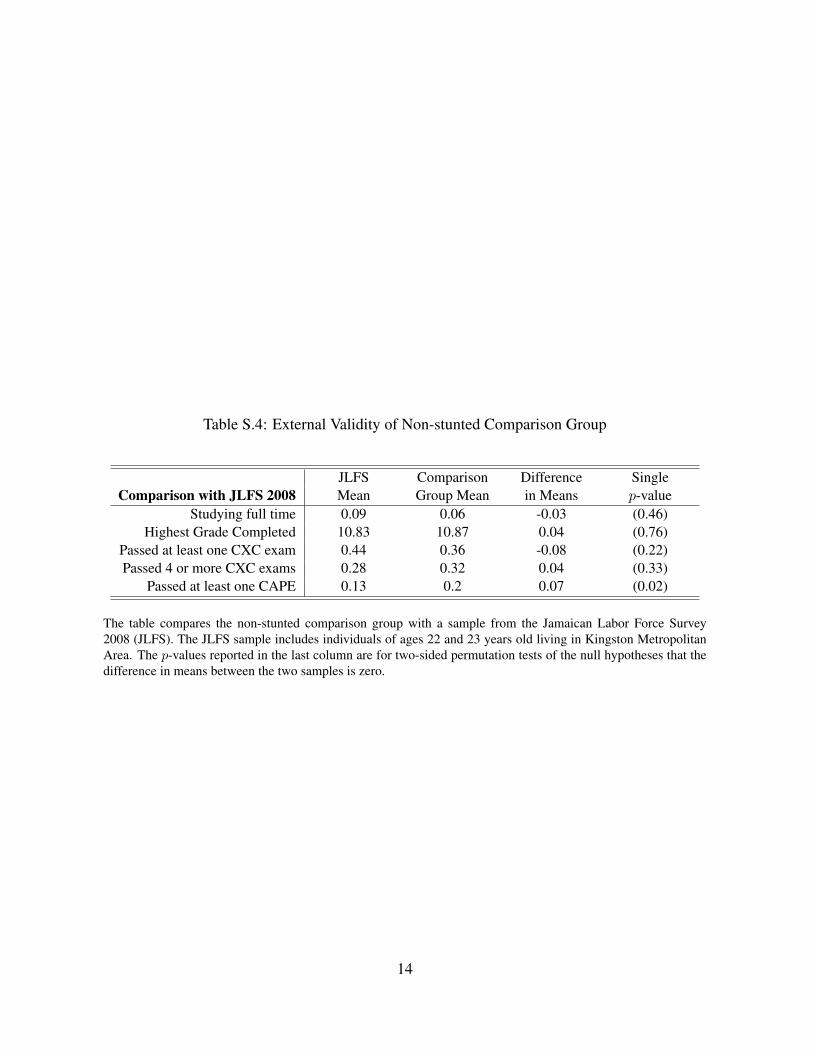
Table S.4: External Validity of Non-stunted Comparison Group

JLFS Comparison Difference SingleComparison with JLFS 2008 Mean Group Mean in Means p-value

Studying full time 0.09 0.06 -0.03 (0.46)Highest Grade Completed 10.83 10.87 0.04 (0.76)

Passed at least one CXC exam 0.44 0.36 -0.08 (0.22)Passed 4 or more CXC exams 0.28 0.32 0.04 (0.33)

Passed at least one CAPE 0.13 0.2 0.07 (0.02)

The table compares the non-stunted comparison group with a sample from the Jamaican Labor Force Survey2008 (JLFS). The JLFS sample includes individuals of ages 22 and 23 years old living in Kingston MetropolitanArea. The p-values reported in the last column are for two-sided permutation tests of the null hypotheses that thedifference in means between the two samples is zero.

14

Tabl

eS.

5:C

atch

Up

-Com

pari

son

ofed

ucat

ion

and

skill

sfo

rthe

Non

-stu

nted

and

stun

ted

trea

tmen

tsam

ples

Non

-stu

nted

-tre

atm

ent

NTr

eatm

ent

Mea

nβ

Non

-stu

nted

Sing

lep

-Val

ueSD

p-V

alue

A.S

choo

ling

Tota

lyea

rsof

educ

atio

n11

411

.45

-0.1

1(0

.63)

[0.8

7]A

nyvo

catio

nalt

rain

ing

118

0.68

-0.0

8(0

.78)

[0.9

2]A

nyco

llege

118

0.13

0.01

(0.3

8)[0

.74]

Insc

hool

118

0.26

-0.0

2(0

.57)

[0.8

6]In

scho

olfu

lltim

e11

80.

19-0

.08

(0.8

8)[0

.88]

B.E

xam

sPa

ssed

atle

asto

neC

XC

exam

106

0.33

0.20

(0.0

1)[0

.03]

Pass

ed4

orm

ore

CX

Cex

ams

106

0.22

0.14

(0.0

5)[0

.09]

Pass

edat

leas

tone

CA

PE10

60.

090.

01(0

.37)

[0.3

7]C

.Cog

nitiv

eSk

illsa

t18

year

sold

WR

AT

Mat

h11

231

.46

2.44

(0.0

1)[0

.04]

WR

AT

Rea

ding

112

19.6

74.

10(0

.01)

[0.0

3]R

eadi

ng-c

ompr

ehen

sion

112

9.52

1.70

(0.0

2)[0

.04]

PPV

T11

298

.85

9.63

(0.0

2)[0

.04]

Ver

balA

nalo

gies

112

8.96

2.26

(0.0

0)[0

.01]

Rav

ens

Mat

rice

s11

229

.60

3.25

(0.0

5)[0

.05]

WA

ISIQ

112

72.1

74.

97(0

.01)

[0.0

3]D

.Soc

io-e

mot

iona

lski

llsat

18ye

arso

ldO

ppos

ition

albe

havi

or(i

nver

ted)

112

-6.0

20.

27(0

.34)

[0.5

0]C

ogni

tive

Prob

lem

s/In

atte

ntio

n(i

nv.)

112

-5.6

5-0

.37

(0.5

6)[0

.56]

Hyp

erac

tivity

(inv

.)11

2-4

.40

1.11

(0.0

6)[0

.15]

Anx

iety

(inv

.)11

2-1

3.60

0.80

(0.2

6)[0

.41]

Dep

ress

ion

(inv

.)11

2-5

.81

0.11

(0.4

3)[0

.43]

Self

-est

eem

(inv

.)11

225

.63

0.74

(0.2

7)[0

.35]

The

tabl

epr

esen

tses

timat

esof

the

diff

eren

cein

educ

atio

nan

dsk

ills

betw

een

the

wei

ghte

dno

n-st

unte

dco

mpa

riso

ngr

oup

and

the

stun

ted

cogn

itive

stim

ulat

ion

grou

p.O

urp

-val

ues

are

foro

ne-s

ided

bloc

kpe

rmut

atio

nte

sts

ofth

enu

llhy

poth

esis

ofco

mpl

ete

catc

h-up

onea

chou

tcom

e(s

ingl

ep

-val

ue,

inpa

rent

hese

s)an

dac

coun

ting

for

mul

tiple

hypo

thes

es(s

tepd

ownp

-val

ues,

inbr

acke

ts).

Perm

utat

ion

bloc

ksar

eba

sed

onge

nder

only

,but

dono

tco

ntro

lfor

diff

eren

ces

inba

selin

eva

lues

beca

use

the

aim

isto

test

for

catc

h-up

desp

iteth

ein

itial

disa

dvan

tage

.Tr

eatm

entm

ean

isth

em

ean

ofth

est

unte

dgr

oup

rece

ivin

gco

gniti

vest

imul

atio

n.T

heβ

isth

eco

effic

ient

forb

eing

inth

eno

nst

unte

dgr

oup

afte

rrew

eigh

ting

the

data

with

IPW

toco

rrec

tfo

rattr

ition

.Exa

ms

have

asm

alle

rsam

ple

size

beca

use

they

are

only

cons

ider

edfo

rtho

sew

hodi

dno

tmig

rate

orm

igra

ted

afte

rtur

ning

18ye

ars

old.

Skill

sha

vebe

enin

vert

edfo

ropp

ositi

onal

beha

vior

,cog

nitiv

epr

oble

ms,

anxi

ety,

depr

essi

onso

that

they

are

posi

tivel

yco

ded.

15

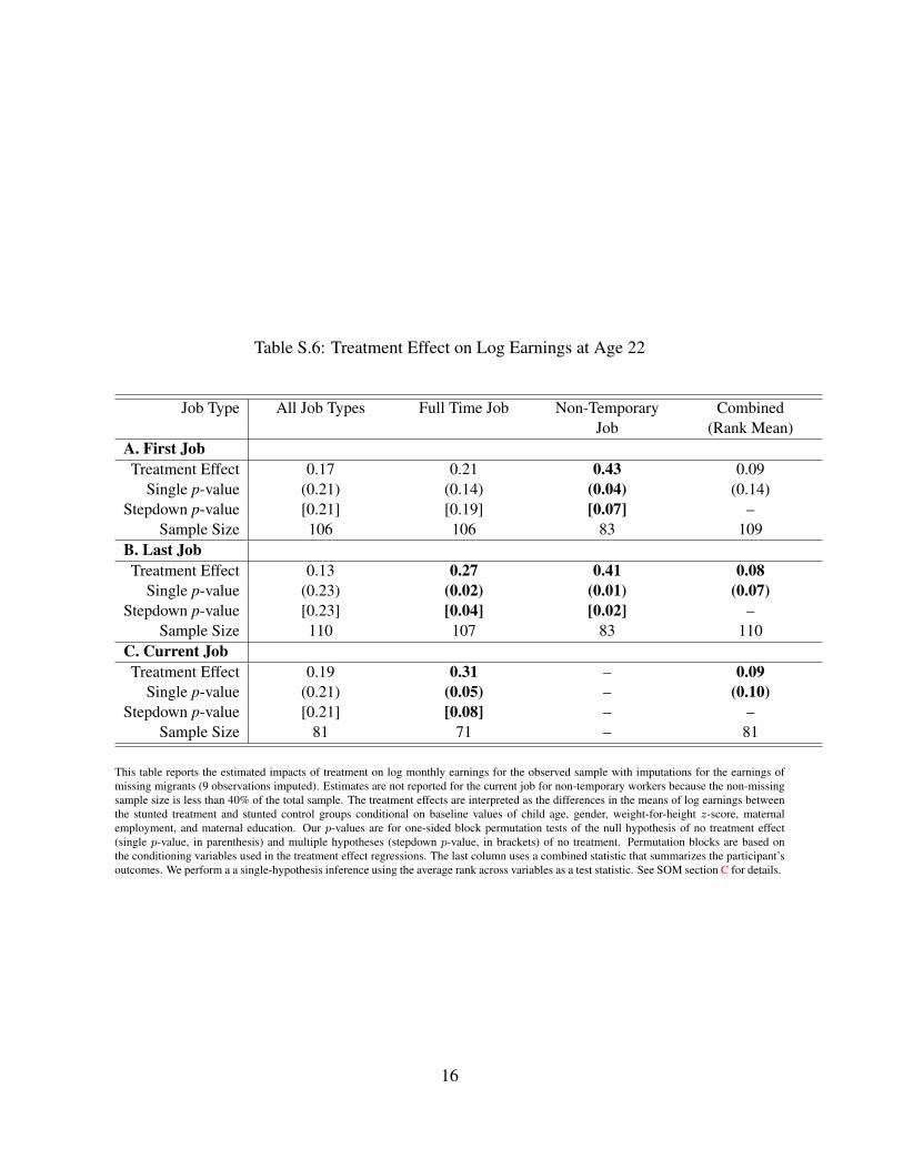
Table S.6: Treatment Effect on Log Earnings at Age 22


A. First JobTreatment Effect 0.17 0.21 0.43 0.09

Single p-value (0.21) (0.14) (0.04) (0.14)Stepdown p-value [0.21] [0.19] [0.07] –

Sample Size 106 106 83 109B. Last JobTreatment Effect 0.13 0.27 0.41 0.08


Sample Size 110 107 83 110C. Current JobTreatment Effect 0.19 0.31 – 0.09

Single p-value (0.21) (0.05) – (0.10)Stepdown p-value [0.21] [0.08] – –

Sample Size 81 71 – 81

This table reports the estimated impacts of treatment on log monthly earnings for the observed sample with imputations for the earnings ofmissing migrants (9 observations imputed). Estimates are not reported for the current job for non-temporary workers because the non-missingsample size is less than 40% of the total sample. The treatment effects are interpreted as the differences in the means of log earnings betweenthe stunted treatment and stunted control groups conditional on baseline values of child age, gender, weight-for-height z-score, maternalemployment, and maternal education. Our p-values are for one-sided block permutation tests of the null hypothesis of no treatment effect(single p-value, in parenthesis) and multiple hypotheses (stepdown p-value, in brackets) of no treatment. Permutation blocks are based onthe conditioning variables used in the treatment effect regressions. The last column uses a combined statistic that summarizes the participant’soutcomes. We perform a a single-hypothesis inference using the average rank across variables as a test statistic. See SOM section C for details.

16

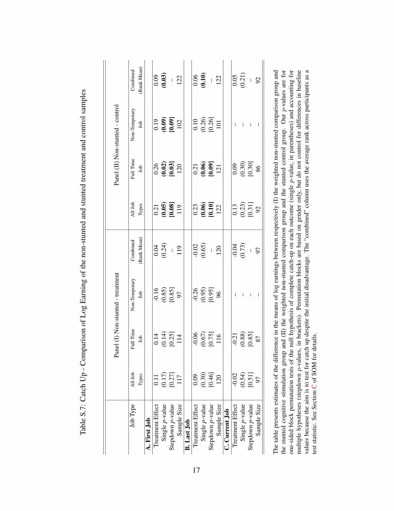
Tabl

eS.

7:C

atch

Up

-Com

pari

son

ofL

ogE

arni

ngof

the

non-

stun

ted

and

stun

ted

trea

tmen

tand

cont

rols

ampl

es

Pane

l(I)

Non

-stu

nted

-tre

atm

ent

Pane

l(II

)Non

-stu

nted

-con

trol

Job

Type

All

Job

Full

Tim

eN

on-T

empo

rary

Com

bine

dA

llJo

bFu

llTi

me

Non

-Tem

pora

ryC

ombi

ned

Type

sJo

bJo

b(R

ank

Mea

n)Ty

pes

Job

Job

(Ran

kM

ean)

A.F

irst

Job

Trea

tmen

tEff

ect

0.11

0.14

-0.1

60.

040.

210.

260.

190.

09Si

ngle

p-va

lue

(0.1

7)(0

.14)

(0.8

5)(0

.24)

(0.0

5)(0

.02)

(0.0

9)(0

.03)

Step

dow

np-

valu

e[0

.27]

[0.2

5][0

.85]

–[0

.08]

[0.0

3][0

.09]

–Sa

mpl

eSi

ze11

711

497

119

119

120

102

122

B.L

astJ

obTr

eatm

entE

ffec

t0.

09-0

.06

-0.2

6-0

.02

0.23

0.21

0.10

0.06

Sing

lep-

valu

e(0

.30)

(0.6

7)(0

.95)

(0.6

5)(0

.06)

(0.0

6)(0

.26)

(0.1

0)St

epdo

wn

p-va

lue

[0.4

6][0

.75]

[0.9

5]–

[0.1

0][0

.09]

[0.2

6]–

Sam

ple

Size

120

116

9612

012

212

110

112

2C

.Cur

rent

Job

Trea

tmen

tEff

ect

-0.0

2-0

.21

–-0

.04

0.13

0.09

–0.

05Si

ngle

p-va

lue

(0.5

4)(0

.88)

–(0

.73)

(0.2

3)(0

.30)

–(0

.21)

Step

dow

np-

valu

e[0

.51]

[0.8

5]–

–[0

.31]

[0.3

0]–

–Sa

mpl

eSi

ze97

87–

9792

86–

92

The

tabl

epr

esen

tses

timat

esof

the

diff

eren

cein

the

mea

nsof

log

earn

ings

betw

een

resp

ectiv

ely

(I)

the

wei

ghte

dno

n-st

unte

dco

mpa

riso

ngr

oup

and

the

stun

ted

cogn

itive

stim

ulat

ion

grou

pan

d(I

I)th

ew

eigh

ted

non-

stun

ted

com

pari

son

grou

pan

dth

est

unte

dco

ntro

lgr

oup.

Ourp

-val

ues

are

for

one-

side

dbl

ock

perm

utat

ion

test

sof

the

null

hypo

thes

isof

com

plet

eca

tch-

upon

each

outc

ome

(sin

glep

-val

ue,i

npa

rent

hese

s)an

dac

coun

ting

for

mul

tiple

hypo

thes

es(s

tepd

ownp

-val

ues,

inbr

acke

ts).

Perm

utat

ion

bloc

ksar

eba

sed

onge

nder

only

,but

dono

tco

ntro

lfo

rdi

ffer

ence

sin

base

line

valu

esbe

caus

eth

eai

mis

tote

stfo

rca

tch

upde

spite

the

initi

aldi

sadv

anta

ge.

The

“com

bine

d”co

lum

nus

esth

eav

erag

era

nkac

ross

part

icip

ants

asa

test

stat

istic

.See

Sect

ion

Cof

SOM

ford

etai

ls.

17

C Methodology

We investigate two questions; (1) What is the impact of the stimulation treatment on earnings and (2) Does treat-

ment enable the stunted treatment group to catch-up with the non-stunted comparison group? We estimate the

treatment effect on earnings in the experimental stunted sample by linear regression controlling for the variables

used in the randomization protocol (age and sex). The catch-up analysis compares the non-stunted comparison

group with the stunted treatment group. We estimate the catch-up effects using linear regression also controlling

for age and gender.

The small sample size of the Jamaican Study suggests that classical statistical procedures that rely on large

sample asymptotic theory to justify the distribution of test statistics may be misleading. We address this problem

by using non-parametric permutation tests as implemented in (21). Permutation tests are valid in small samples

because they are distribution free and do not rely on assumptions about the parametric sampling distribution.

The structure of the randomization protocol requires us to permute within the age-sex strata blocks used for the

initial randomization. For the treatment effect analysis we expand the number of strata blocks to include the other

variables not balanced at baseline.

Increasing the number of blocks of permutations reduces the number of participants that share the same values

of the conditioning variables. This may render some permutation blocks invalid as some blocks may contain only

treatments or only controls. Effectively, we lose those observations as the treatment status does not vary within

this block. To avoid this problem, we apply a parsimonious selection of conditioning covariates in which we only

add new covariates besides the ones used in the randomization protocol variables if they significantly explain the

outcome of interest. Specifically, we perform a linear regression in which the outcome of interest is explained by

the treatment status, the baseline variables used in the randomization protocol and additional variables we ought

to examine. We only include the additional variables if we are able to reject the null hypothesis that equates the

linear coefficient of the variable being examined to zero. We perform the inference using a double-sided bootstrap

p-value and we adopt a significance level of 5%.

Application of the block-permutation test is straightforward for discrete variables, but it requires discretization

of continuous variables. Weight-for-height is the only variable that we had to discretize. We chose the largest

possible number of divisions that maximize the minimum number of observations in a block. This led us to divide

the sample in three categories, those with a z-score higher than 0, those less than 0 but greater than -2, and those

less than -2 in the standardized weight for height distribution. We lost no observations for the permutation analysis

18

by following this rule.

The presence of multiple outcomes leads to the potential danger of arbitrarily selecting “statistically signifi-

cant” outcomes where high values of test statistics arise by chance. Testing each hypothesis one at a time with a

fixed significance increases the probability of a type-I error exponentially as the number of outcomes tested grows.

We correct for this potential source of bias in inference by performing multiple hypothesis testing based on the

Family-Wise Error Rate (FWER), which is the probability of rejecting at least one true null Hypothesis. We use

the stepdown algorithm proposed in (50), which generates inference exhibiting strong FWER control. Associated

with each outcome is a single null hypothesis of no treatment effect. We implement the stepdown procedure for

conceptually similar blocks of outcomes.

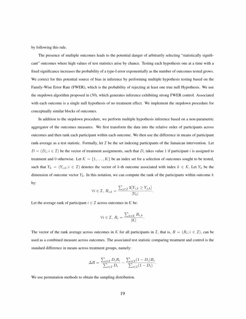
In addition to the stepdown procedure, we perform multiple hypothesis inference based on a non-parametric

aggregator of the outcomes measures. We first transform the data into the relative order of participants across

outcomes and then rank each participant within each outcome. We then use the difference in means of participant

rank-average as a test statistic. Formally, let I be the set indexing participants of the Jamaican intervention. Let

D = (Di; i ∈ I) be the vector of treatment assignments, such that Di takes value 1 if participant i is assigned to

treatment and 0 otherwise. Let K = {1, . . . ,K} be an index set for a selection of outcomes sought to be tested,

such that Yk = (Yi,k; i ∈ I) denotes the vector of k-th outcome associated with index k ∈ K. Let Yk be the

dimension of outcome vector Yk. In this notation, we can compute the rank of the participants within outcome k

by:

∀i ∈ I, Ri,k =

∑j∈I 1[Yi,k ≥ Yj,k]

|Yk|.

Let the average rank of participant i ∈ I across outcomes in K be:

∀i ∈ I, Ri =

∑k∈KRi,k

|K|.

The vector of the rank average across outcomes in K for all participants in I, that is, R = (Ri; i ∈ I), can be

used as a combined measure across outcomes. The associated test statistic comparing treatment and control is the

standard difference in means across treatment groups, namely:

∆R =

∑i∈I DiRi∑i∈I Di

−∑

i∈I(1−Di)Ri∑i∈I(1−Di)

.

We use permutation methods to obtain the sampling distribution.

19

D Robustness Tests

In this section we report the results of several analyses that examine the extent to which the estimates of treatment

on earnings in Table 1 are are robust to a number of assumptions and potential concerns.

We first test the hypothesis that we can pool the stimulation and combined stimulation arms into a single treat-

ment group by estimating the treatment effect on log earnings separately for the pure stimulation intervention and

for the combined stimulation/supplemental intervention. We identify the first by comparing the pure stimulation

group to the pure control group and the second by comparing the combined stimulation/supplementation to the

pure supplementation arm (Tables S.8–S.9). These comparisons ensure that in both cases the only difference be-

tween the treatment and comparison groups is the stimulation intervention. The results presented in Tables S.8–S.9

show that the estimated effect sizes of the two approaches are close to one another in almost all cases.5 Moreover,

we cannot reject the hypothesis that the estimated treatment effects using the stimulation group are equal to the

estimated treatment effect using the combined stimulation/supplementation group in all cases.

Second, we test the hypothesis that there is no effect of nutritional supplementation on log earnings and that

we can pool the supplementation and pure control groups. We estimate the treatment effect on log earnings sep-

arately for the pure supplementation intervention and for the combined stimulation/supplemental intervention by

comparing the pure supplementation group to the pure control group and the second by comparing the combined

stimulation/supplementation to the pure stimulation arm (Tables S.10–S.11). These comparisons ensure that in

each case the only difference between the treatment and comparison groups is the supplementation intervention.

The results presented in Tables S.10–S.11 show that the estimated effect sizes of the two approaches are in gen-

eral close to one another and none are statistically significant. In all cases we cannot reject the null hypothesis

that the estimated treatment effect using the supplementation group is equal to the estimated treatment effect us-

ing the combined stimulation/supplementation group. Finally, we estimate the effect of supplementation on log

earnings by comparing the the pooled supplementation and combined supplementation/stimulation groups to the

pooled stimulation and control groups (SOM Table S.12) and find that none of the estimated effects are statistically

significantly different from zero.

Third, we examine the extent to which the estimates may be affected by censoring in that we only observe

the earnings of those employed who are in the labor force. We estimate the effect of treatment on labor force

5The coefficients are close in 20 out of 22 cases and positive in all cases. Despite the substantially smallersample sizes than in the pooled model, 10 of the estimated effects are significantly different from zero and thecombined rank mean test is statistically significant in 5 out of the 8 cases.

20

participation using the methods discussed in Section C and find that treatment does not appear to affect overall

labor force participation or participation in full or non-temporary jobs (Table S.13). These results are consistent

with negligible bias from censoring in the estimated treatment effects on earnings.

Fourth, we examine the concern that the results might be driven by migrants and therefore sensitive to the

imputations of earnings for the 9 missing migrants. We re-estimate the effect of treatment on log earnings excluding

the migrants (SOM Table S.14) and find that estimated effect sizes remain very close to the original estimates both

in terms of magnitude and and statistical significance.

Finally, we assess the extent to which the IPW correction for baseline imbalance affected the estimates by

re-estimating the effects of treatment on earnings without the IPW weights (SOM Table S.15). Again, we find the

results remain close to the original estimates both in terms of size and significance.

D.1 Empirical Analysis

This appendix reports results of analyses of the robustness of the estimated treatment effects the stimulation on

log earnings reported in Table 1 to assumptions and adjustments. Specifically, this appendix presents evidence to

support (1) the pooling of the stimulation and combined stimulation/supplementation arms into a single treatment

group, (2) that there is that there is no effect of supplementation on earnings, (3) that the estimates are not sensitive

to the treatment of migrants and adjustments to control for imbalances of some characteristics at baseline, and (4)

that there are no statistically significant differences by gender.

D.2 Pooling of Stimulation/Supplementation arms

We estimate the treatment effect of stimulation on log earnings separately for the pure stimulation intervention

and for the combined stimulation/supplemental arm by comparing the pure stimulation group to the pure control

group and the the combined stimulation/supplementation arm to the pure supplementation arm using the methods

described in Section C. These comparisons ensure that in each case the only difference between the treatment and

comparison groups is the stimulation intervention.

We present these results in Tables S.8–S.9. Results for different earnings indicators are reported in panels

A–D. Columns are associated with different job types. Within each panel we first report the results from com-

paring the stimulation group to the control group and then, just below, the results from comparing the combined

stimulation/supplementation group to the supplementation group. Finally, the last row in each panel presents the

21

two-sided p-values for the permutation test of equality of treatment effects estimated with just the pure stimulation

group and estimated with the combined stimulation/supplementation group. The estimated effect sizes of the two

approaches are close to one another in 20 out of 22 cases and positive in all cases. Despite the small sample sizes,

10 estimates are significantly different from zero and the combined rank mean test is statistically significant in

5 out of the 8 cases. However, the stimulation arm of the intervention shows strong results. It does not matter

if we compare stimulation with no treatment or stimulation/suplementation with supplementation only. In both

comparisons we examine a group that has stimulation with a group that does not have the stimulation. In both

cases it shows strong effects of the stimulation treatment. There is weak evidence that nutrition plus stimulation

is more effective for many outcomes than stimulation alone. Finally, in all cases we cannot reject the hypothesis

that the estimated treatment effect using the stimulation group is equal to the estimated treatment effect using the

combined stimulation/supplementation group.

D.3 The Effect of Nutritional Supplementation on Log-earnings

We estimate the treatment effect of supplementation on log earnings separately for the pure supplementation in-

tervention and for the combined stimulation/supplemental intervention by comparing the pure supplementation

group to the pure control group and the combined stimulation/supplementation to the pure stimulation group

(Tables S.10–S.11). These comparisons ensure that in each case the only difference between the treatment and

comparison groups is the supplementation intervention.

Our analysis is presented in Tables S.10–S.11. Results for different earnings indicators are reported in panels

A–D. Columns are associated with different job types. The estimated effect sizes of the two approaches are in

general close to one another and slightly negative. None of the 22 estimated effects are statistically significant nor

are any of the 8 combined rank mean tests (see SOM section C for a description of this statistic). In all cases

we cannot reject the hypothesis that the estimated treatment effect using the supplementation group is equal to the

estimated treatment effect using the combined stimulation/supplementation group.

We also estimate the effect of supplementation on log earnings by comparing the the pooled supplementa-

tion and combined supplementation/stimulation groups to the pooled stimulation and control groups (Table S.12).

None of the estimated effects are significantly different from zero as indicated by the p-values for the individual

coefficient estimates and for the combined rank mean tests.

22

D.4 Adjustments for Migration and Baseline Imbalance

The first 2 tables are used to examine whether the results are sensitive to adjustments for migrants and baseline

imbalances in a few characteristics. Specifically, Table S.14 presents the estimated treatment effects excluding all

migrants from the sample and Table S.15 presents the estimated treatment effects including migrant but not using

IPW weights to correct for baseline imbalance. In both cases, the estimated coefficients remain very close the

estimates in Table 1 in terms of both magnitude and statistical significance.

D.5 Catchup and Migrants

We examine how sensible are our catchup results regarding the subset of stunted migrants. As a robustness check,

we re-estimate the catchup model excluding the migrants in Table S.16. We find results are comparable to Table 2

in terms of significance and magnitude.

D.6 Gender Comparison

We also examine the treatment effects of the stimulation arm of the Jamaican intervention separately by gender.

We estimated the treatment effects separately by gender (Table S.17) in order to assess whether there are gender

differences of the type that have been found in U.S. (21). While the estimated effects on earnings are higher for

males, tests for equality cannot reject the hypothesis that the impact on earnings is equal for males and females.

These results should be considered with caution as the study was neither designed nor powered to assess impact

separately by gender. While the estimated effects on earnings are higher for males, tests for equality cannot reject

the hypothesis that the impact on earnings is equal for males and females.

23

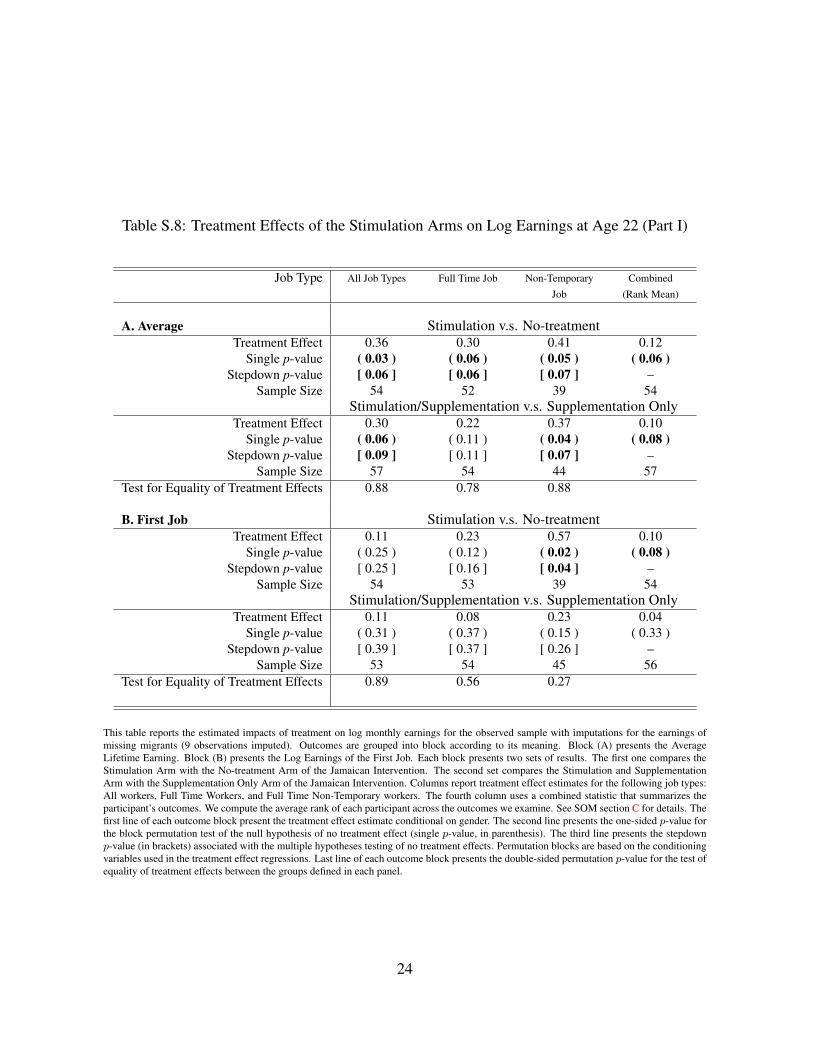
Table S.8: Treatment Effects of the Stimulation Arms on Log Earnings at Age 22 (Part I)

Job Type All Job Types Full Time Job Non-Temporary Combined

Job (Rank Mean)

A. Average Stimulation v.s. No-treatmentTreatment Effect 0.36 0.30 0.41 0.12

Single p-value ( 0.03 ) ( 0.06 ) ( 0.05 ) ( 0.06 )Stepdown p-value [ 0.06 ] [ 0.06 ] [ 0.07 ] –

Sample Size 54 52 39 54Stimulation/Supplementation v.s. Supplementation Only

Treatment Effect 0.30 0.22 0.37 0.10Single p-value ( 0.06 ) ( 0.11 ) ( 0.04 ) ( 0.08 )

Stepdown p-value [ 0.09 ] [ 0.11 ] [ 0.07 ] –Sample Size 57 54 44 57

Test for Equality of Treatment Effects 0.88 0.78 0.88

B. First Job Stimulation v.s. No-treatmentTreatment Effect 0.11 0.23 0.57 0.10



Treatment Effect 0.11 0.08 0.23 0.04Single p-value ( 0.31 ) ( 0.37 ) ( 0.15 ) ( 0.33 )

Stepdown p-value [ 0.39 ] [ 0.37 ] [ 0.26 ] –Sample Size 53 54 45 56


This table reports the estimated impacts of treatment on log monthly earnings for the observed sample with imputations for the earnings ofmissing migrants (9 observations imputed). Outcomes are grouped into block according to its meaning. Block (A) presents the AverageLifetime Earning. Block (B) presents the Log Earnings of the First Job. Each block presents two sets of results. The first one compares theStimulation Arm with the No-treatment Arm of the Jamaican Intervention. The second set compares the Stimulation and SupplementationArm with the Supplementation Only Arm of the Jamaican Intervention. Columns report treatment effect estimates for the following job types:All workers, Full Time Workers, and Full Time Non-Temporary workers. The fourth column uses a combined statistic that summarizes theparticipant’s outcomes. We compute the average rank of each participant across the outcomes we examine. See SOM section C for details. Thefirst line of each outcome block present the treatment effect estimate conditional on gender. The second line presents the one-sided p-value forthe block permutation test of the null hypothesis of no treatment effect (single p-value, in parenthesis). The third line presents the stepdownp-value (in brackets) associated with the multiple hypotheses testing of no treatment effects. Permutation blocks are based on the conditioningvariables used in the treatment effect regressions. Last line of each outcome block presents the double-sided permutation p-value for the test ofequality of treatment effects between the groups defined in each panel.

24

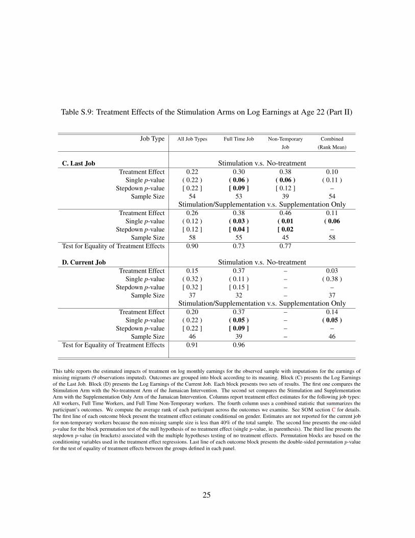
Table S.9: Treatment Effects of the Stimulation Arms on Log Earnings at Age 22 (Part II)


Job (Rank Mean)

C. Last Job Stimulation v.s. No-treatmentTreatment Effect 0.22 0.30 0.38 0.10



Treatment Effect 0.26 0.38 0.46 0.11Single p-value ( 0.12 ) ( 0.03 ) ( 0.01 ( 0.06

Stepdown p-value [ 0.12 ] [ 0.04 ] [ 0.02 –Sample Size 58 55 45 58


D. Current Job Stimulation v.s. No-treatmentTreatment Effect 0.15 0.37 – 0.03

Single p-value ( 0.32 ) ( 0.11 ) – ( 0.38 )Stepdown p-value [ 0.32 ] [ 0.15 ] – –

Sample Size 37 32 – 37Stimulation/Supplementation v.s. Supplementation Only

Treatment Effect 0.20 0.37 – 0.14Single p-value ( 0.22 ) ( 0.05 ) – ( 0.05 )

Stepdown p-value [ 0.22 ] [ 0.09 ] – –Sample Size 46 39 – 46

Test for Equality of Treatment Effects 0.91 0.96

This table reports the estimated impacts of treatment on log monthly earnings for the observed sample with imputations for the earnings ofmissing migrants (9 observations imputed). Outcomes are grouped into block according to its meaning. Block (C) presents the Log Earningsof the Last Job. Block (D) presents the Log Earnings of the Current Job. Each block presents two sets of results. The first one compares theStimulation Arm with the No-treatment Arm of the Jamaican Intervention. The second set compares the Stimulation and SupplementationArm with the Supplementation Only Arm of the Jamaican Intervention. Columns report treatment effect estimates for the following job types:All workers, Full Time Workers, and Full Time Non-Temporary workers. The fourth column uses a combined statistic that summarizes theparticipant’s outcomes. We compute the average rank of each participant across the outcomes we examine. See SOM section C for details.The first line of each outcome block present the treatment effect estimate conditional on gender. Estimates are not reported for the current jobfor non-temporary workers because the non-missing sample size is less than 40% of the total sample. The second line presents the one-sidedp-value for the block permutation test of the null hypothesis of no treatment effect (single p-value, in parenthesis). The third line presents thestepdown p-value (in brackets) associated with the multiple hypotheses testing of no treatment effects. Permutation blocks are based on theconditioning variables used in the treatment effect regressions. Last line of each outcome block presents the double-sided permutation p-valuefor the test of equality of treatment effects between the groups defined in each panel.

25

Table S.10: Treatment Effects of the Supplementation Arms on Log Earnings at Age 22 (Part I)


Job (Rank Mean)

A. Average Supplementation v.s. No-treatmentTreatment Effect -0.12 -0.11 -0.05 -0.06

Single p-value 0.73 0.71 0.59 0.78Stepdown p-value 0.73 0.78 0.70 –

Sample Size 55 54 43 55Stimulation/Supplementation v.s. Stimulation Only

Treatment Effect -0.17 -0.18 -0.10 -0.07Single p-value 0.83 0.84 0.67 0.81

Stepdown p-value 0.90 0.84 0.82 –Sample Size 56 52 40 56


B. First Job Supplementation v.s. No-treatmentTreatment Effect -0.11 -0.11 0.07 -0.04



Treatment Effect -0.11 -0.26 -0.27 -0.10Single p-value 0.79 0.91 0.89 0.94



This table reports the estimated impacts of treatment on log monthly earnings for the observed sample with imputations for the earnings ofmissing migrants (9 observations imputed). Outcomes are grouped into block according to its meaning. Block (A) presents the AverageLifetime Earning. Block (B) presents the Log Earnings of the First Job. Each block presents two sets of results. The first one compares theStimulation Arm with the No-treatment Arm of the Jamaican Intervention. The second set compares the Stimulation and SupplementationArm with the Supplementation Only Arm of the Jamaican Intervention. Columns report treatment effect estimates for the following job types:All workers, Full Time Workers, and Full Time Non-Temporary workers. The fourth column uses a combined statistic that summarizes theparticipant’s outcomes. We compute the average rank of each participant across the outcomes we examine. See SOM section C for details. Thefirst line of each outcome block present the treatment effect estimate conditional on gender. The second line presents the one-sided p-value forthe block permutation test of the null hypothesis of no treatment effect (single p-value, in parenthesis). The third line presents the stepdownp-value (in brackets) associated with the multiple hypotheses testing of no treatment effects. Permutation blocks are based on the conditioningvariables used in the treatment effect regressions. Last line of each outcome block presents the double-sided permutation p-value for the test ofequality of treatment effects between the groups defined in each panel.

26

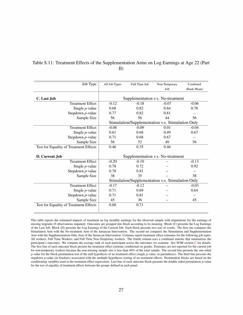
Table S.11: Treatment Effects of the Supplementation Arms on Log Earnings at Age 22 (PartII)


Job (Rank Mean)

C. Last Job Supplementation v.s. No-treatmentTreatment Effect -0.12 -0.18 -0.07 -0.06



Treatment Effect -0.08 -0.09 0.01 -0.04Single p-value 0.61 0.68 0.49 0.67



D. Current Job Supplementation v.s. No-treatmentTreatment Effect -0.20 -0.10 – -0.13

Single p-value 0.78 0.72 – 0.92Stepdown p-value 0.78 0.81 – –

Sample Size 38 35 – 38Stimulation/Supplementation v.s. Stimulation Only

Treatment Effect -0.17 -0.12 – -0.03Single p-value 0.71 0.69 – 0.64

Stepdown p-value 0.71 0.81 – –Sample Size 45 36 – 45

Test for Equality of Treatment Effects 0.68 0.71

This table reports the estimated impacts of treatment on log monthly earnings for the observed sample with imputations for the earnings ofmissing migrants (9 observations imputed). Outcomes are grouped into block according to its meaning. Block (C) presents the Log Earningsof the Last Job. Block (D) presents the Log Earnings of the Current Job. Each block presents two sets of results. The first one compares theStimulation Arm with the No-treatment Arm of the Jamaican Intervention. The second set compares the Stimulation and SupplementationArm with the Supplementation Only Arm of the Jamaican Intervention. Columns report treatment effect estimates for the following job types:All workers, Full Time Workers, and Full Time Non-Temporary workers. The fourth column uses a combined statistic that summarizes theparticipant’s outcomes. We compute the average rank of each participant across the outcomes we examine. See SOM section C for details.The first line of each outcome block present the treatment effect estimate conditional on gender. Estimates are not reported for the current jobfor non-temporary workers because the non-missing sample size is less than 40% of the total sample. The second line presents the one-sidedp-value for the block permutation test of the null hypothesis of no treatment effect (single p-value, in parenthesis). The third line presents thestepdown p-value (in brackets) associated with the multiple hypotheses testing of no treatment effects. Permutation blocks are based on theconditioning variables used in the treatment effect regressions. Last line of each outcome block presents the double-sided permutation p-valuefor the test of equality of treatment effects between the groups defined in each panel.

27

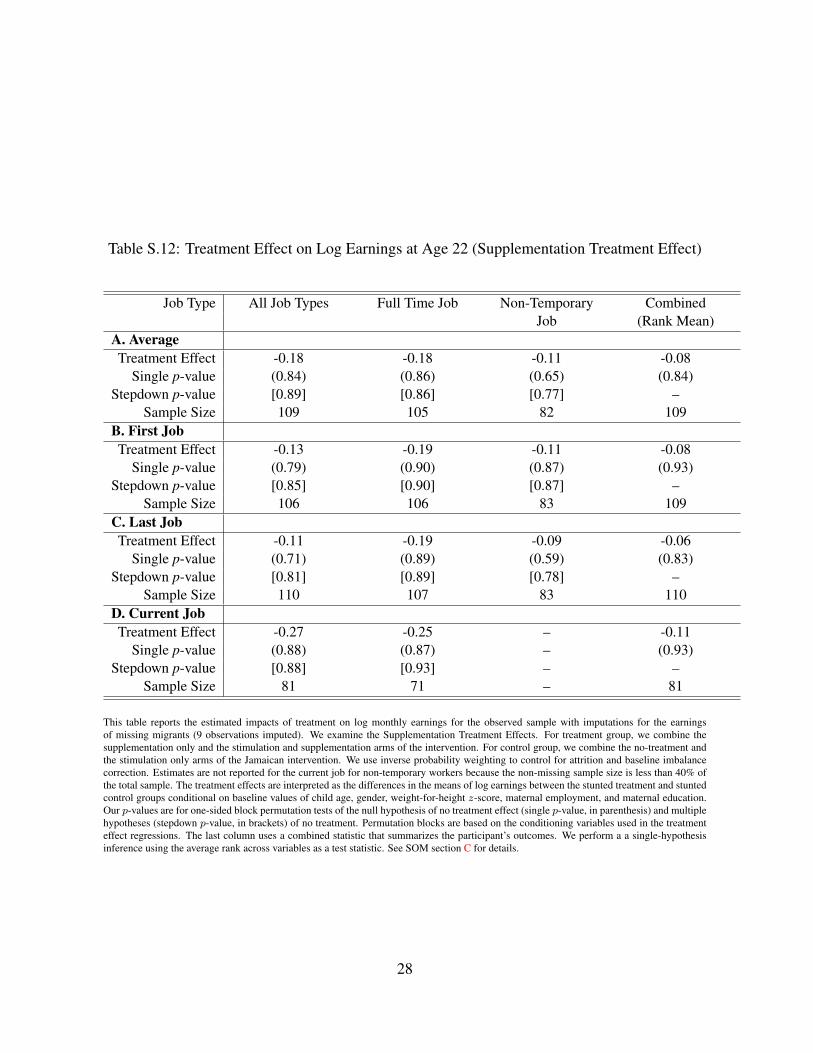
Table S.12: Treatment Effect on Log Earnings at Age 22 (Supplementation Treatment Effect)


A. AverageTreatment Effect -0.18 -0.18 -0.11 -0.08


Sample Size 109 105 82 109B. First JobTreatment Effect -0.13 -0.19 -0.11 -0.08


Sample Size 106 106 83 109C. Last JobTreatment Effect -0.11 -0.19 -0.09 -0.06


Sample Size 110 107 83 110D. Current JobTreatment Effect -0.27 -0.25 – -0.11



This table reports the estimated impacts of treatment on log monthly earnings for the observed sample with imputations for the earningsof missing migrants (9 observations imputed). We examine the Supplementation Treatment Effects. For treatment group, we combine thesupplementation only and the stimulation and supplementation arms of the intervention. For control group, we combine the no-treatment andthe stimulation only arms of the Jamaican intervention. We use inverse probability weighting to control for attrition and baseline imbalancecorrection. Estimates are not reported for the current job for non-temporary workers because the non-missing sample size is less than 40% ofthe total sample. The treatment effects are interpreted as the differences in the means of log earnings between the stunted treatment and stuntedcontrol groups conditional on baseline values of child age, gender, weight-for-height z-score, maternal employment, and maternal education.Our p-values are for one-sided block permutation tests of the null hypothesis of no treatment effect (single p-value, in parenthesis) and multiplehypotheses (stepdown p-value, in brackets) of no treatment. Permutation blocks are based on the conditioning variables used in the treatmenteffect regressions. The last column uses a combined statistic that summarizes the participant’s outcomes. We perform a a single-hypothesisinference using the average rank across variables as a test statistic. See SOM section C for details.

28

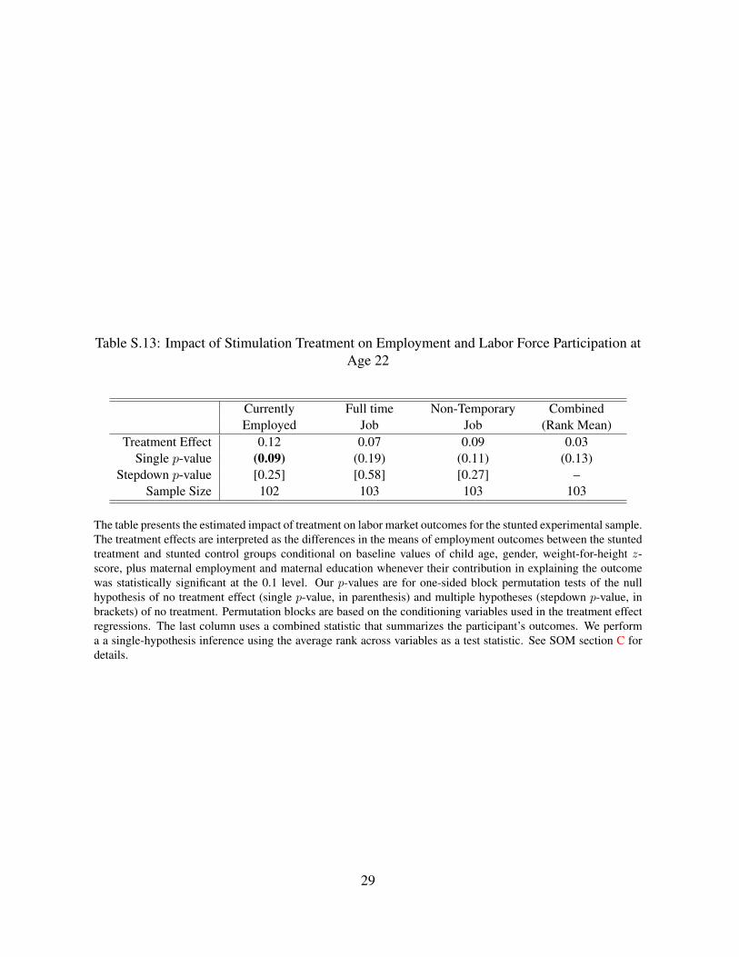
Table S.13: Impact of Stimulation Treatment on Employment and Labor Force Participation atAge 22

Currently Full time Non-Temporary CombinedEmployed Job Job (Rank Mean)


Stepdown p-value [0.25] [0.58] [0.27] –Sample Size 102 103 103 103

The table presents the estimated impact of treatment on labor market outcomes for the stunted experimental sample.The treatment effects are interpreted as the differences in the means of employment outcomes between the stuntedtreatment and stunted control groups conditional on baseline values of child age, gender, weight-for-height z-score, plus maternal employment and maternal education whenever their contribution in explaining the outcomewas statistically significant at the 0.1 level. Our p-values are for one-sided block permutation tests of the nullhypothesis of no treatment effect (single p-value, in parenthesis) and multiple hypotheses (stepdown p-value, inbrackets) of no treatment. Permutation blocks are based on the conditioning variables used in the treatment effectregressions. The last column uses a combined statistic that summarizes the participant’s outcomes. We performa a single-hypothesis inference using the average rank across variables as a test statistic. See SOM section C fordetails.

29

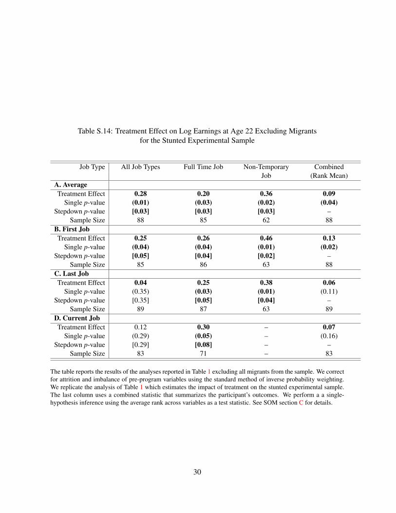
Table S.14: Treatment Effect on Log Earnings at Age 22 Excluding Migrantsfor the Stunted Experimental Sample


A. AverageTreatment Effect 0.28 0.20 0.36 0.09


Sample Size 88 85 62 88B. First JobTreatment Effect 0.25 0.26 0.46 0.13


Sample Size 85 86 63 88C. Last JobTreatment Effect 0.04 0.25 0.38 0.06


Sample Size 89 87 63 89D. Current JobTreatment Effect 0.12 0.30 – 0.07



The table reports the results of the analyses reported in Table 1 excluding all migrants from the sample. We correctfor attrition and imbalance of pre-program variables using the standard method of inverse probability weighting.We replicate the analysis of Table 1 which estimates the impact of treatment on the stunted experimental sample.The last column uses a combined statistic that summarizes the participant’s outcomes. We perform a a single-hypothesis inference using the average rank across variables as a test statistic. See SOM section C for details.

30

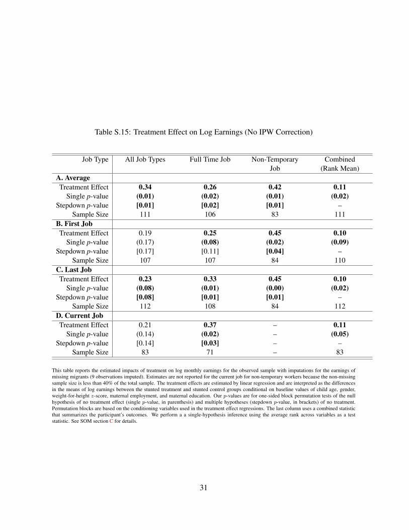
Table S.15: Treatment Effect on Log Earnings (No IPW Correction)


A. AverageTreatment Effect 0.34 0.26 0.42 0.11


Sample Size 111 106 83 111B. First JobTreatment Effect 0.19 0.25 0.45 0.10


Sample Size 107 107 84 110C. Last JobTreatment Effect 0.23 0.33 0.45 0.10


Sample Size 112 108 84 112D. Current JobTreatment Effect 0.21 0.37 – 0.11



This table reports the estimated impacts of treatment on log monthly earnings for the observed sample with imputations for the earnings ofmissing migrants (9 observations imputed). Estimates are not reported for the current job for non-temporary workers because the non-missingsample size is less than 40% of the total sample. The treatment effects are estimated by linear regression and are interpreted as the differencesin the means of log earnings between the stunted treatment and stunted control groups conditional on baseline values of child age, gender,weight-for-height z-score, maternal employment, and maternal education. Our p-values are for one-sided block permutation tests of the nullhypothesis of no treatment effect (single p-value, in parenthesis) and multiple hypotheses (stepdown p-value, in brackets) of no treatment.Permutation blocks are based on the conditioning variables used in the treatment effect regressions. The last column uses a combined statisticthat summarizes the participant’s outcomes. We perform a a single-hypothesis inference using the average rank across variables as a teststatistic. See SOM section C for details.

31

Tabl

eS.

16:C

atch

Up

-Com

pari

son

ofL

ogE

arni

ngE

xclu

ding

Mig

rant

sfo

rthe

Non

-stu

nted

and

stun

ted

trea

tmen

tand

cont

rols

ampl

es

Pane

l(I)

Non

-stu

nted

-tre

atm

ent

Pane

l(II

)Non

-stu

nted

-con

trol

Job

Type

All

Job

Full

Tim

eN

on-T

empo

rary

Com

bine

dA

llJo

bFu

llTi

me

Non

-Tem

pora

ryC

ombi

ned

Type

sJo

bJo

b(R

ank

Mea

n)Ty

pes

Job

Job

(Ran

kM

ean)

A.A

vera

geTr

eatm

entE

ffec

t0.

030.

02-0

.09

0.04

0.24

0.17

0.16

0.09

Sing

lep-

valu

e(0

.40)

(0.4

4)(0

.73)

(0.2

8)(0

.04)

(0.0

9)(0

.15)

(0.0

2)St

epdo

wn

p-va

lue

[0.5

3][0

.50]

[0.7

3]–

[0.0

6][0

.11]

[0.1

5]–

Sam

ple

Size

9794

7597

103

101

8310

3B

.Fir

stJo

bTr

eatm

entE

ffec

t0.

110.

17-0

.01

0.07

0.23

0.30

0.24

0.11

Sing

lep-

valu

e(0

.20)

(0.0

9)(0

.52)

(0.1

1)(0

.04)

(0.0

1)(0

.02)

(0.0

1)St

epdo

wn

p-va

lue

[0.2

9][0

.17]

[0.5

2]–

[0.0

2][0

.04]

[0.0

4]–

Sam

ple

Size

9492

7596

101

102

8410

4C

.Las

tJob

Trea

tmen

tEff

ect

0.24

0.01

-0.1

30.

030.

270.

220.

130.

08Si

ngle

p-va

lue

(0.1

0)(0

.48)

(0.7

8)(0

.32)

(0.0

4)(0

.05)

(0.2

0)(0

.07)

Step

dow

np-

valu

e[0

.19]

[0.5

7][0

.78]

–[0

.08]

[0.0

8][0

.20]

–Sa

mpl

eSi

ze97

9474

9710

410

383

104

D.C

urre

ntJo

bTr

eatm

entE

ffec

t0.

12-0

.14

–0.

010.

160.

10–

0.05

Sing

lep-

valu

e(0

.28)

(0.7

6)–

(0.4

4)(0

.20)

(0.2

8)–

(0.2

3)St

epdo

wn

p-va

lue

[0.3

7][0

.76]

––

[0.2

8][0

.28]

––

Sam

ple

Size

7567

–75

7771

–77

The

tabl

ere

port

sth

ere

sults

ofth

ean

alys

esre

port

edin

Tabl

e2

excl

udin

gal

lmig

rant

sfr

omth

esa

mpl

e.W

eco

rrec

tfor

attr

ition

and

imba

lanc

eof

pre-

prog

ram

vari

able

sus

ing

the

stan

dard

met

hod

ofin

vers

epr

obab

ility

wei

ghtin

g.W

ere

plic

ate

the

anal

ysis

ofTa

ble

2w

hich

estim

ates

the

impa

ctof

trea

tmen

ton

the

non-

stun

ted

expe

rim

enta

lsam

ple.

Defi

nitio

nsar

eas

give

nin

Tabl

e2.

32

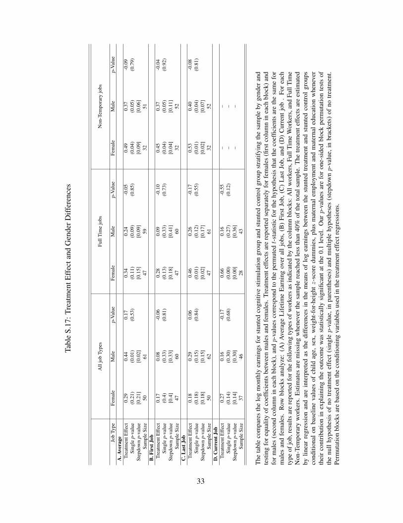
Tabl

eS.

17:T

reat

men

tEff

ecta

ndG

ende

rDiff

eren

ces

All

job

Type

sFu

llTi

me

jobs

Non

-Tem

pora

ryjo

bs

Job

Type

Fem

ale

Mal

ep

-Val

ueFe

mal

eM

ale

p-V

alue

Fem

ale

Mal

ep

-Val

ueA

.Ave

rage

Trea

tmen

tEff

ect

0.29

0.44

0.17

0.34

0.24

-0.0

50.

490.

37-0

.09

Sing

lep-

valu

e(0

.21)

(0.0

1)(0

.53)

(0.1

1)(0

.09)

(0.8

5)(0

.04)

(0.0

5)(0

.79)

Step

dow

np-

valu

e[0

.21]

[0.0

2][0

.15]

[0.0

9][0

.09]

[0.0

6]Sa

mpl

eSi

ze50

6147

5932

51B

.Fir

stJo

bTr

eatm

entE

ffec

t0.

170.

08-0

.06

0.28

0.09

-0.1

00.

450.

37-0

.04

Sing

lep-

valu

e(0

.4)

(0.3

3)(0

.81)

(0.1

3)(0

.33)

(0.7

3)(0

.04)

(0.0

5)(0

.92)

Step

dow

np-

valu

e[0

.4]

[0.3

3][0

.18]

[0.4

1][0

.04]

[0.1

1]Sa

mpl

eSi

ze47

6047

6032

52C

.Las

tJob

Trea

tmen

tEff

ect

0.18

0.29

0.06

0.46

0.26

-0.1

70.

530.

40-0

.08

Sing

lep-

valu

e(0

.18)

(0.1

5)(0

.84)

(0.0

1)(0

.12)

(0.5

5)(0

.01)

(0.0

4)(0

.81)

Step

dow

np-

valu

e[0

.18]

[0.1

5][0

.02]

[0.1

7][0

.02]

[0.0

7]Sa

mpl

eSi

ze50

6247

6132

52D

.Cur

rent

Job

Trea

tmen

tEff

ect

0.27

0.16

-0.1

70.

660.

16-0

.55

––

Sing

lep-

valu

e(0

.14)

(0.3

0)(0

.68)

(0.0

0)(0

.27)

(0.1

2)–

–St

epdo

wn

p-va

lue

[0.1

4][0

.30]

[0.0

0][0

.36]

––

Sam

ple

Size

3746

2843

The

tabl

eco

mpa

res

the

log

mon

thly

earn

ings

for

stun

ted

cogn

itive

stim

ulat

ion

grou

pan

dst

unte

dco

ntro

lgro

upst

ratif

ying

the

sam

ple

byge

nder

and

test

ing

fore

qual

ityof

coef

ficie

nts

betw

een

mal

esan

dfe

mal

es.

Trea

tmen

teff

ects

are

repo

rted

sepa

rate

lyfo

rfem

ales

(firs

tcol

umn

inea

chbl

ock)

and

for

mal

es(s

econ

dco

lum

nin

each

bloc

k),a

ndp

-val

ues

corr

espo

ndto

the

perm

utedt-

stat

istic

for

the

hypo

thes

isth

atth

eco

effic

ient

sar

eth

esa

me

for

mal

esan

dfe

mal

es.

Row

bloc

ksan

alyz

e:(A

)A

vera

geL

ifet

ime

Ear

ning

over

all

jobs

,(B

)Fi

rst

Job,

(C)

Las

tJob

,and

(D)

Cur

rent

job

.Fo

rea

chty

peof

job,

resu

ltsar

ere

port

edfo

rthe

follo

win

gty

pes

ofw

orke

rsas

indi

cate

dby

the

colu

mn

bloc

ks:A

llw

orke

rs,F

ullT

ime

Wor

kers

,and

Full

Tim

eN

on-T

empo

rary

wor

kers

.E

stim

ates

are

mis

sing

whe

neve

rth

esa

mpl

ere

ache

dle

ssth

an40

%of

the

tota

lsam

ple.

The

trea

tmen

teff

ects

are

estim

ated

bylin

ear

regr

essi

onan

dar

ein

terp

rete

das

the

diff

eren

ces

inth

em

eans

oflo

gea

rnin

gsbe

twee

nth

est

unte

dtr

eatm

ent

and

stun

ted

cont

rol

grou

psco

nditi

onal

onba

selin

eva

lues

ofch

ildag

e,se

x,w

eigh

t-fo

r-he

ightz

-sco

redu

mm

ies,

plus

mat

erna

lem

ploy

men

tan

dm

ater

nal

educ

atio

nw

hene

ver

thei

rco

ntri

butio

nin

expl

aini

ngth

eou

tcom

ew

asst

atis

tical

lysi

gnifi

cant

atth

e0.

1le

vel.

Ourp

-val

ues

are

for

one-

side

dbl

ock

perm

utat

ion

test

sof

the

null

hypo

thes

isof

notr

eatm

ente

ffec

t(si

nglep

-val

ue,i

npa

rent

hese

s)an

dm

ultip

lehy

poth

eses

(ste

pdow

np

-val

ue,i

nbr

acke

ts)

ofno

trea

tmen

t.Pe

rmut

atio

nbl

ocks

are

base

don

the

cond

ition

ing

vari

able

sus

edin

the

trea

tmen

teff

ectr

egre

ssio

ns.

33

E Construction of Earnings Variables

Income data consist of participant reported salaries for each job. The employment survey is job-specific: questions

targeted each job separately. Only jobs with positive earnings are considered in our analysis.

In each job, it was asked how many months per year, weeks per months and days per week is the person

usually working in that job. Using this data, we classify a job as full time if the participant had at least 20 working

days per month. We classify the job as nontemporary and full time if the participant worked full time at least 8

months per year.

We compute total salary for each job by multiplying the total number of months worked by the monthly salary

indicated for the job being analyzed. We then divided the overall sum by the number of months worked in total.

Average earnings full time is calculated as the sum over all of the full time jobs of monthly earnings multiplied by

the number of months spent in each of those jobs , over the sum of all months spent in a full time job.

We also apply a temporal criteria for job classification. Namely, we classify jobs into first, current and last

jobs according to employment history of the participant. If two jobs ended in the same year the one yielding the

highest earnings was assumed to be the last job. Current job is equal to last job if the person is currently employed.

First job is assumed to be the earliest job that ended. If more than one job ended in that year, we define first job as

the job with longest duration.

The propensity score is the estimated probability of being in the attrited group at the 22 years old wave. It

has been calculated based on three separate models targeting the following samples: (1) stunted treatment group,

(2) stunted control group and (3) non-stunted comparison group. Each model was chosen to maximize the Akaike

information criteria. The models for the stunted treatment group and for the stunted control group include baseline

variables. The majority of the children in the non-stunted comparison group had been added at the 7-years-old

follow-up surveys. Thus, the model for the non-stunted comparison group include data from that wave, which is

the earliest complete data available.

We use a linear model to impute earning values for missing data regarding migrant workers. Imputation

targeted those migrant workers who were lost to follow-up. In the stunted group, these totals of 9 workers. The

imputation was obtained through a linear prediction based on selected set of baseline covariates.The small sample

size of the data demands a parsimonious covariate selection, which were chosen in order to maximize the Akaike

information criteria. Selected covariates are: migrant status, sex and treatment group indicator (for the stunted

group) and on migrant status and sex (for non-stunted group).

34

Documents

Labor Market Returns to an Early Childhood Stimulation