Embed Size (px)
Citation preview

Lab Revising 101:
Revise, Rework, Revamp
A Senior Research Project by:
Jessica Vance
Collaborated with:
Melissa Zoller
Advised by:
Professor Jan Chaloupka
April 20, 2007

Lab Revising 101: Revise, Rework, Revamp
Table of Contents
Objective and Overview …………………………………………………………. p. 1
Purpose …………………………………………………………………………... p. 2
Achievements …………………………………………………………………………… p. 6
Introductory Sections and General Improvements ….. ………………………. p. 6
Lab 3: Motion with Constant Acceleration …………………………………… p. 8
Lab 4: Vectors ………………………………………………………………… p. 9
Lab 7: Conservation of Linear Momentum ……………………………………. p. 10
Lab 8: Conservation of Energy (Disk and Block on Track) ……………………. p. 12
Conclusions ……………………………………………………………………………. p. 15
Lab 7: Conservation of Linear Momentum ……………………………………. p. 15
Lab 8: Conservation of Energy (Disk and Block on Track) ……………………. p. 32
Final Thoughts …………………………………………………………………………… p. 39
Appendix A: Lab Manual ……………………………………………………………. p. 40
Introduction to Physics 101 Labs ……………………………………………. p. 40
Sample Lab Format ……………………………………………………………. p. 41
Notes about the Lab Report ……………………………………………………. p. 43
Microsoft Excel How-To ……………………………………………………. p. 44
Lab 3: Motion with Constant Acceleration ……………………………………. p. 46
Lab 3 Program Requirements and Sample Run-Through ………………………. p. 51
Lab 4: Vectors and Forces ……………………………………………………. p. 56
Lab 7: Conservation of Linear Momentum ……………………………………. p. 61
Lab 8: Conservation of Energy (Disk and Block on Track) ……………………. p. 74
Appendix B: Physics 101 Lab Evaluation ……………………………………………. p. 80
Appendix C: Works Cited ……………………………………………………………. p. 81

1
Lab Revising 101: Revise, Rework, Revamp
Objective and Overview
The objective of this Senior Research Project is to reorganize, rewrite, and reinvigorate
the Physics 101 Labs. By improving the organizational structure of the manual, cutting down on
superfluous and unnecessary information provided in the laboratory, rewriting current labs, and
in some cases creating entirely new labs, we hope to improve the efficiency and effectiveness of
the Physics 101 Labs. Laboratory experience and learning is, and should be, an integral part of
science education; however, as the labs are presented in the current system, they are not as
conducive to student learning as they need to be.
Originally, the intent was to create an entirely new lab manual. However, given the
incredibly daunting task that this would entail, it was decided, upon conferring with Professor
Chaloupka, that a more readily attainable goal would be to create two original labs and edit two
more. I believe we have succeeded beyond anyone’s expectations, including my own, in this
project. We have rewritten or heavily revised four labs; of those, we have tested two on current
Physics 101 students, who then completed surveys that gave qualitative and quantitative
responses to the labs.1 These tests were pertinent to this project because it allowed for additional
improvement of the new labs before they were finalized for this project. Moreover, having
current Physics 101 students test these labs allowed us to determine what students with similar
levels of experience and education in physics would learn from performing these labs.
Furthermore, we have outlined the design for a new computer program that would revolutionize
how labs are instructed and performed today. We have also succeeded in changing the focus of
the labs. No longer are students expected to learn the material after they leave the lab and
1 See Physics 101 Lab Evaluation, Appendix B.

2
express it in lab reports. In these new labs, the focus is shifted toward student learning in the
laboratory itself, with conceptual questions and room for data analysis and calculations in the
manual. This provides students with the opportunity to learn in the lab itself rather than in their
dorm rooms.
Purpose
According to the current laboratory manual, students perform laboratory experiments
because, “by performing hands-on experiments [one is] able to explore and confirm (or disprove)
the concepts which scientists have put forth to describe the processes that govern our world.”2
Furthermore, according to John Carnduff and Norman Reid, “the laboratory provides a setting
for training not only in practical hand and instrument skills but also for many of the thinking,
planning, recording, interpreting and group working skills that a degree course must include.”3
Laboratory experiments should clarify information presented in lecture and further students’
understanding of physical concepts, properties, theories, and laws. Indeed, some basic physical
ideas—for example, that gravity is a constant on Earth’s surface—are not intuitive for the non-
scientist. Without laboratory experiments or some other form of visual or physical
demonstration, the information is not easily conveyed. The primary focus of an introductory lab
class, then, should be the physical activity of performing the lab itself rather than writing the
report afterward. Although report writing is a fundamental necessity of scientific research, it
should not be the main focus in a beginner lab course.
2 Laboratory Manual: General Physics 101, The College of William and Mary, 2006, iv. 3 John Carnduff and Norman Reid. Enhancing undergraduate chemistry laboratories: Pre-laboratory and post-laboratory exercises, (London: Royal Society of Chemistry, 2003), ii.

3
Indeed, “according to the American Association of Physics Teachers, the important goals
of introductory physics laboratories should be designing experimental investigations, evaluating
experimental data, and developing the ability to work in groups.”4 Although students in a 101
lab setting will not be able to design their own experiments, the labs should provide the mental
stimulation necessary for them to come up with further experiments, if they so choose, or at the
very least, enable them to transfer the concepts they learn in the lab to their lecture class.
Furthermore, the interactive skills learned by working in a group setting, even if with just one
other person, are of prime importance to the student’s future. A lab, if it is designed well, may
help further the critical thinking and communication skills of the students.5 In order for any of
this to be possible, however, the lab manual must be of high quality. Indeed, as A.H. Johnstone,
A. Watt, and T.U. Zaman note:
“there is no point in putting a student into…a lecture course without mental
preparation…The student has to be aware of what the lab is about, what the
background theory is, what techniques are required, what kind of things to expect
in light of the theory, so that the unexpected, when it occurs, will be evident.”6
The current lab manual, however, fails to reach these expectations and standards. Its
language is too formal and hard to read, let alone understand. Rather than encouraging the study
of physics, many students are turned away by the dryness of the language. Physics is a very
difficult field to study, let alone master. The problem many undergraduates face is that the
professors’ knowledge of physics is so far beyond their scope of understanding; there is a
seemingly impenetrable barrier between what the professor knows and what the student hopes to
learn. The manual, as it is currently written, only further exploits such a sentiment. It makes far
4 Eugenia Etkina, Sahana Murthy, and Xueli Zou “Using introductory labs to engage students in experimental design,” American Journal of Physics, 74 (November 2006): 979. 5Anne J. Cox and William F. Junkin, “Enhanced student learning in the introductory physics laboratory,” Physics Education 37, no.1 (2002): 40. 6 A.H. Johnstone, A. Watt, and T.U. Zaman, "The students’ attitude and cognition change to a physics laboratory,"
Centre for Science Education 33, no. 1 (1998): 23-24.

4
too many assumptions as to what the student knows, and the background information it does
provide is written in a way that makes it difficult to understand. Furthermore, the organization of
the manual is confusing and, at times, frustrating. Instructions on how to operate equipment, in
particular the Data Studio computer program, are scattered throughout the manual. Earlier
directions, no matter how helpful or pertinent, are never referenced again. Repeating, or even
better centralizing the instructions, would provide students with easier access to them and allow
them to better understand how to utilize the equipment. Furthermore, the manual is full of
typographical and grammatical errors that can easily be remedied by a good revision, one we
hope to have partially provided. Some of the labs are simply outdated; with the current
technological improvements, there may be more efficient or effective ways to teach the concepts
to students. For that matter, there may also be more creative ways to demonstrate the physical
concepts rather than what is currently designed.
The lab manual, furthermore, places far too much focus on the lab report at the expense
of the physical concepts themselves. According to the Investigative Science Learning
Environment, students learn best when they design their own experiments to investigate
phenomena, test explanations of these, and then apply the explanations to realistic problems.
Reports, one should note, are not a part of this process.7 Although lab reports are integral to
sharing physics research, they are often impractical at the introductory level. Far too often,
students do not understand why they are writing lab reports. Worse still, they get absolutely
nothing out of the experience. Lab reports are subjectively graded by teaching assistants (TAs)
who all too often put more focus on the format of the report than what the students learn in the
lab. Our plan is to incorporate more worksheets into the lab manual that can be completed
during the lab period and submitted to the TAs before students leave. Data will still be collected
7 Etkina, et. al., 979.
5
and analyzed, calculations performed, and conclusions drawn; the only difference is that students
will not have to write lab reports. Furthermore, we have incorporated more questions into the
labs to encourage students to think analytically, so as to ensure conceptual understanding and
foster critical thinking skills.
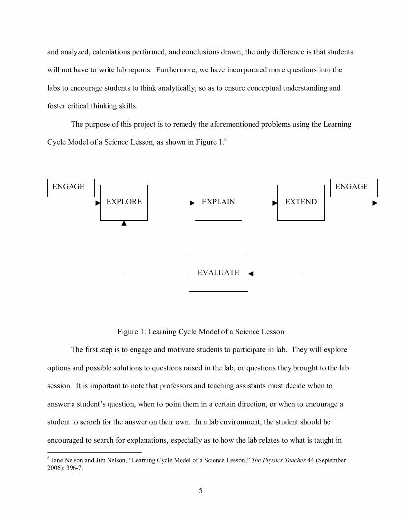
The purpose of this project is to remedy the aforementioned problems using the Learning
Cycle Model of a Science Lesson, as shown in Figure 1.8
Figure 1: Learning Cycle Model of a Science Lesson
The first step is to engage and motivate students to participate in lab. They will explore
options and possible solutions to questions raised in the lab, or questions they brought to the lab
session. It is important to note that professors and teaching assistants must decide when to
answer a student’s question, when to point them in a certain direction, or when to encourage a
student to search for the answer on their own. In a lab environment, the student should be
encouraged to search for explanations, especially as to how the lab relates to what is taught in
8 Jane Nelson and Jim Nelson, “Learning Cycle Model of a Science Lesson,” The Physics Teacher 44 (September
2006): 396-7.
EXPLORE EXPLAIN EXTEND
ENGAGE ENGAGE
EVALUATE

6
lecture. After all, “definitions and other concepts arise out of the experience rather than from
textbook or lecture.”9 Following this process of searching for explanations, students are then
encouraged to elaborate (or extend) upon what they have learned by discovering further
applications, then evaluate what they have learned before beginning to explore physics again.
This step may need to be initiated or instigated by TAs, especially when dealing with reluctant
students. Throughout this cycle, students need to be motivated and encouraged to continue their
studies. Labs must play a role in this, as they provide the only hands-on method of education
provided in a science curriculum. Students must be kept engaged and enthusiastic throughout
the process in order for an adequate education to be obtained.
Achievements
Introductory Sections and General Improvements
The original lab manual had a very weak introduction section. It was densely and poorly
worded and did not adequately convey the purpose of the Physics 101 labs. The new
introduction details the importance of physics education and lab experiences in general by
describing how the experiences in lab will help prepare students to be better informed and more
pro-active citizens in a world that is increasingly becoming scientifically centered.10
Furthermore, because so many students are inexperienced in writing labs before taking this
course, a sample lab format has been added to the text of the manual.11
It gives the standard
layout of a lab write-up, as well as explicit details of what should be included in the report. Each
section is explicitly broken-down and its components detailed, as well as what should not be
9 Nelson and Nelson, 397. 10 See Introduction to Physics Labs, Appendix A. 11 See Lab Format, Appendix A.

7
included in the report. The purpose of this section is to standardize the reports so that
experienced researchers are not given an initial advantage in writing lab reports. To further help
with this endeavor, a list of hints about writing the report is also included.12
These pointers,
although obvious and repetitive to experienced lab writers, are designed to help beginning
students perfect their formatting skills. Additionally, a section on using Microsoft Excel, at the
request of current TAs, will be added, following the advice of TAs that some students do not
know how to use this invaluable program.13
Additionally, general changes were made to each lab we rewrote. Conceptual questions
have become a mainstay in the new labs. As the American Journal of Physics notes, “putting
guiding questions in all write-ups… [to] require students to focus on the same elements of the
experimental design and communication.”14
These are designed to encourage immediate student
comprehension of the lab and also provide suggestions of what information should be detailed in
the lab report. As the Anne Cox and William Junkin’s study shows, these questions enhance
student comprehension of the physical concepts presented in the lab.15
Furthermore, the
information sections were elaborated upon and more derivation of equations were shown to
enhance comprehension and decrease the possibility of student confusion. Space was provided
to record data, particularly constants and values needed for calculations, at the bequest of current
TAs. Furthermore, more space was provided for calculations to be performed in lab. All these
changes are designed to enhance comprehension of the material presented.
12 See Notes about the Lab Report, Appendix A. 13 See Microsoft Excel How-To, Appendix A. 14 Etkina, et.al., 980. 15 Cox and Junkin, 39-41.

8
Lab 3: Motion with Constant Acceleration
This completely original lab is this project’s greatest leap from the status quo.16
Going in
to this research project, a goal was to decrease the number of labs using the air table; although a
good tool in theory, it is a tedious, difficult to work with piece of equipment. The air table is
inadequate to demonstrate how universal constant acceleration is. The air table makes it appear
that constant acceleration can only happen in certain restrained circumstances. The average
beginning physics student cannot realize the power and importance, if not omnipotence, of
constant acceleration. The new lab will focus much more on hands-on education, so that by
increasing student enthusiasm and attention in the lab will increase retention of the material.
Students will stand in front of a black screen that has been demarcated using a grid and
toss a ball in a parabolic arch back and forth to each other. Using a high-speed digital camera
coupled with a strobe light, a third person will take pictures of the trajectory of the ball. In this
photograph, the ball will appear each time the strobe light flashes, forming a parabola-shaped
trajectory. Students will then download these images to a computer, and use a computer
program to measure the height and position of the ball at various points in its trajectory. Using
this data, students use this computer program, complete with the basic kinematics equations, to
determine the initial velocity of the ball and the angle at which it was released. An outline of this
program, which we have named Kinematics Manipulation, has been designed; these designs and
a sample output are displayed in Appendix A.17
What is spectacular about this redesigned lab is that it makes visual a concept so
fundamental, and yet so hard to grasp, in physics: that the path of a ball tossed in the air is a
parabola. As the Lab 3 Program Requirements in the Appendix A show, the camera
16 See Lab 3: Motion with Constant Acceleration, Appendix A. 17 See Lab 3 Program Requirements and Sample Run Through, Appendix A.

9
perfectly captures this arc of the ball. Even students (and a certain professor) who have
studied physics for years were shocked and excited about how perfect of an arc the object’s
trajectory was. Having first-year physics students study and analyze this data would cement
this knowledge and allow them to further understand and appreciate the nuances of the
subject. Moreover, the new and original format of this lab would capture student attention
and encourage them to continue their studies in physics.
Lab 4: Vectors and Forces
The original lab format relied far too heavily on the force table to demonstrate the two-
dimensional nature of forces. Although the force table itself is an ingenious facet for suggesting
the relationship between forces, the current lab did not allow for the fact that students did not
have to make any calculations or intuitions in balancing the table.18
They could simply guess-
and-check by moving the strings holding weights around the table until it achieved equilibrium.
Although we recognize that this could take a long while without a good deal of luck, we also
know that many students will prefer this tedious way to having to perform any sort of
calculations on their own. To counteract that tendency, we chose to restrict the students’ options.
In both trials of the lab, either all the positions of the strings or all the masses are fixed or strictly
limited by rules. For example, when the masses are restricted, they must follow
CBA mmm 2== (1)
One of the set of variables that is not completely restricted will be the value the student solves
for to balance the force table. The catch in all of this is that the student is not allowed to touch
the force table until they complete the calculations in the space provided in the manual. The
18 See Lab 4: Vectors and Forces, Appendix A.
10
ultimate hope is that the TA will witness the first, and only, time the final mass and/or string is
put into place. Points will not necessarily have to be taken off if mistakes are made, that is
entirely at the discretion of the TA, but we want to quash the guess-and-check method of
experimentation currently in practice.
Furthermore, an additional section in this lab tests what students learned in the lab. By
making them measure the distance between two points in Small Hall (values which will be
entirely at the discretion of the TA) with only a string and a protractor, students will be
challenged both creatively and intellectually. They will not have the opportunity to consult
textbooks, but rather will have to apply their knowledge of vectors immediately, in a hands-on
and unique way that will enhance their overall knowledge of this incredibly important and
pertinent idea. This new section replaces what was in the original lab a section devoted to
explaining mathematical calculations of vectors. We felt that students in Physics 101, which is a
calculus-based physics course, should have had enough experience working with and
manipulating vectors that any time spent on this subject in lab would be wasted and ultimately
ineffective.
Lab 7: Conservation of Linear Momentum
From previous experience and talking with students, the most significant problem with
the original lab format was that the lab was simply too tedious and complicated. Although we
agreed that the lab set-up is the best available presently, minor changes to the procedure and
hints on how to achieve adequate results on the trial were added in our reworking of it.19
Furthermore, we sought to improve the effectiveness of the educational component of the lab by
19 See Lab 7: Conservation of Linear Momentum, Appendix A.

11
altering the organization and language of the informational sections. The informational sections
were separated and interspersed throughout the lab so that students would read the background
material immediately before performing that part of the experiment and could easily reference it
as needed. Furthermore, these rewritten informational sections were more concise and easy to
follow so students could understand them step-by-step. The additional conceptual questions
forced students to stay on track of what they should be learning while encouraging them to reach
their own conclusions. The included data sections gave students space to record their data and
perform calculations, thereby ensuring that they would not forget to complete part of the
necessary data collection or calculations. This section also allowed them to check their work
while in the lab, and helped the TAs in the grading process.
Once we had our new Lab 7, we set about testing our new style of lab formatting on
students. It was important to test this particular lab because of its reputation of being unpopular
among the students and generally ineffective. The best way to test our new ideas and verify that
they were in fact more educational and effective in the lab was to test them on an original lab we
recognized already had faults. We ran three tests during lab sessions in the shortened week after
Fall Break, when students did not have their normal labs. The students completed our lab before
they performed the original one in their manual, so as to ensure that they were unbiased when
they tested our model. After each trial, some alterations were made on the labs. After the first,
the conceptual questions were numbered and bolded so students would know they were supposed
to answer them in their lab books and not simply ponder them. After the second trial, we
realized that the students had not covered momentum yet in class, and so many of them did not
yet understand
mvp = (2)

12
We added Equation (2) to the informational sections and a bit more background information on
the concept of momentum to ensure that students, no matter how much material they had covered
in lecture, would be able to follow the lab. No changes were made to the lab after the third trial,
because there were no student outcries for assistance.
The following week, after the students had completed the lab as designed in the current
manual, I visited the 101 lecture and asked those present to fill out a survey on what they thought
of that lab. This survey was very similar to that which students completed after testing the new
labs, except that it also asked them information about the amount of time they spent working on
the lab report. This group would serve as our control group to determine the effectiveness of our
new style of lab.
Lab 8: Conservation of Energy (Disk and Block on Track)
Although conservation of energy is an incredibly important, and indeed fundamental,
topic in physics, the original lab manual did not allow for maximum retention of information.
First, it did not introduce translational motion at all and focused solely on rotational motion.
Excluding translational motion from observation and study in lab denies the student the
opportunity to compare the two forms of motion and understand that translational is explicitly a
part of rotational. The lab also relied on complex and repeated manipulations of equations to
ultimately determine the rate of acceleration of a ball rolling down an inclined track.
21
sin
Mr
I
ga
+
=θ
(3)
This obscure value is shown in Equation (3), where M is the mass of the disk and r is the radius
of the disk’s axle. Students were expected to use the motion detector and Data Studio to

13
determine the acceleration of the disk and then compare the experimental and theoretical values.
The third problem with the original lab format was that it provided directions for Science
Workshop, the previous computer program, rather than the Data Studio program used today.
What was most problematic about this lab, however, was that it did not allow students to
understand conservation of energy. By relying on the obscure Equation (3), with little guidance
as to how the writers of the manual determined such an equation, the students are force-fed the
material at the expense of their own digestion and comprehension of it. Introductory labs should
be designed to perk interest in the material, present the information in a comprehensive and easy-
to-follow manner, and allow the students to develop intuition about fundamental physical
concepts. Many introductory physics classes across the country replicate, or at the very least
discuss, Galileo’s simultaneous dropping of the feather and ball to demonstrate that gravity is a
universal constant; after seeing this performed, students recognize it and add this kernel of
wisdom to their physical intuition that will become quite necessary as they move further through
the field.
The new conservation of energy lab demonstrates both translational and rotational motion
in a manner that will not drastically increase the time spent in lab.20
Both forms of motion are
thoroughly described and explained, and the calculations are listed quite explicitly so that
students can follow along rather than just jump to the final answer. Furthermore, the relationship
between rotational and translational motion is repeated several times throughout the introductory
sections so that students can understand the exact circumstances necessary for the two to be
linked the way they are in this lab. The set-up of the lab is the same, albeit with the addition of a
block of some sort that will first slide down the track. After many trials with erasers, boxes of
chalk, and textbooks, we found that scientific calculators worked adequately, but that another
20 See Lab 8: Conservation of Energy (Disk and Block on Track), Appendix A.
14
smoother and more uniform piece of equipment would be the best object to use. The most
optimal, in our opinion, would be a stainless steel or heavy plastic rectangular box or object of
some sort with a rather substantial mass. An unintended consequence, however, of using a block
as well as a disk on the track, is that the incline of the track for the block must be substantially
higher. we found this was best maintained when the wooden blocks available on Room 107
were placed under the track.
This new format also requires that students pay greater attention to detail, as the angle of
the track, length used in the trial, and mass of the moving object may all vary between the two
parts of the lab. Furthermore, the explicit Data Studio instructions allow the students to rely on
themselves and not the teaching assistants’ help to perform the calculations and create the
graphs, thereby increasing their self-reliance while decreasing the pressure on TAs. Moreover,
the conceptual questions asked in the lab report, as noted before, force students to consider and
comprehend physical concepts while they perform the lab. Lastly, the shift in what is measured
from acceleration to velocity allows students to work with a value that is more familiar and
relatable to them, as well as one that is used more frequently in energy conservation situations.
In general, this new format takes a similar idea to what was used before and expands what is
being demonstrated and taught, changes the manner in which it is demonstrated, asks students to
study a different value, and makes general improvements in the structure and format of the lab.

15
Conclusions
Lab 7
We found that students responded favorably to our new lab format, even given the fact
that the material was unfamiliar to many before they performed the lab. Although we did hear a
fair share of complaints about the length of the lab, many were quite pleased that they would not
have to write a lab report. The quantitative survey answers for the redesigned lab are listed in
Table 1; students were asked to answer the questions on a scale of 1 through 5, with 1 denoting
“very good” and 5 denoting “very bad.” Students were also given the opportunity to provide
qualitative feedback—what they liked and did not like about the lab, what seemed especially
confusing, and what about the new lab was most useful or enjoyable to them.
Q 1 Q 2 Q 3 Q 4 Q 5
Score
Number Respon-dents Score
Number Respon-dents Score
Number Respon-dents Score
Number Respon-dents Score
Number Respon-dents
1 13 1 6 1 9 1 13 1 14
2 15 2 20 2 18 2 11 2 11
3 6 3 9 3 7 3 11 3 5
4 4 4 2 4 5 4 3 4 8
5 2 5 3 5 1 5 2 5 2
Table 1: Collected Data from Surveys for New Lab 7
In total, forty students tested our redesigned lab. The results, for the most part, were
quite favorable. On average, 26 students (or 65% of the test group) rated this lab in the top two
categories, either “somewhat good” or “very good.” Furthermore, the percentage of students
who felt that this redesigned lab was “very bad” was a mere 5%.

16
Figure 2 below graphically portrays student answers to the first question, which asked
students to compare the layout of this lab to other labs they have completed in the past. The few
dissenters expressed dissatisfaction with the fact that all the informational sections were
interspersed with the lab itself; however, most students responded positively because it allowed
for easier access to and better comprehension of the material. The statistics prove this: the mean
response to Question 1 was a 2.2 with a standard deviation of 1.3. Clearly, most students were
genuinely pleased with the new layout of this lab.
Response to Question 1: How was the layout of this lab
compared to other labs you have done?
0
2
4
6
8
10
12
14
16
18
20
22
24
26
28
30
32
34
36
38
40
1 2 3 4 5
Answer
Nu
mb
er
of
Res
po
ns
es
Figure 2: Cumulative Responses to Question 1 for New Lab

17
Similarly, Figure 3 below demonstrates that the procedures in the refined lab were clear
and easy to understand. Those students who ranked us poorly were tested in the first trial, when
many of the kinks were still being worked out of the format. After making improvements in
language and sentence syntax, the students in the latter two trials reported scores of no worse
than three. As Figure 3 suggests, a vast majority of the students (35 out of 40 polled) felt the
procedures were clear. Understanding the procedures allowed students to better comprehend not
only what they were supposed to do in the experiments but the presented material as well. The
mean score was a 2.4, with a standard deviation of 1.0.
Response to Question 2: How clear were the procedures?
0
2
4
6
8
10
12
14
16
18
20
22
24
26
28
30
32
34
36
38
40
1 2 3 4 5
Answer
Nu
mb
er
of
Stu
den
ts
Figure 3: Cumulative Response to Question 2 for New Lab

18
Furthermore, Figure 4 below suggests that students were fairly pleased with the order in
which the information was presented. The mean response was 2.4 with a standard deviation of
1.0. Very few students were openly dissatisfied with the order of information presented in the
lab. Many expressed satisfaction with the fact that the organization of the lab now enabled them
to better understand the material being presented; indeed, just under half of all students surveyed
ranked the helpfulness of the order of information as “somewhat good.” They were able to
understand the concepts while actually in the lab, rather than having to wait until they struggled
through a lab report in the hope of actually learning something. Furthermore, they did not have
to keep flipping back and forth in the lab manual looking for the necessary information; the
material was provided directly before the experiment, allowing for easy access.
Response to Question 3: How did the order that the
information was presented in aid your understanding of the
lab?
0
2
4
6
8
10
12
14
16
18
20
22
24
26
28
30
32
34
36
38
40
1 2 3 4 5
Answer
Nu
mb
er
of
Stu
de
nts
Figure 4: Cumulative Response to Question 3 for New Lab
19
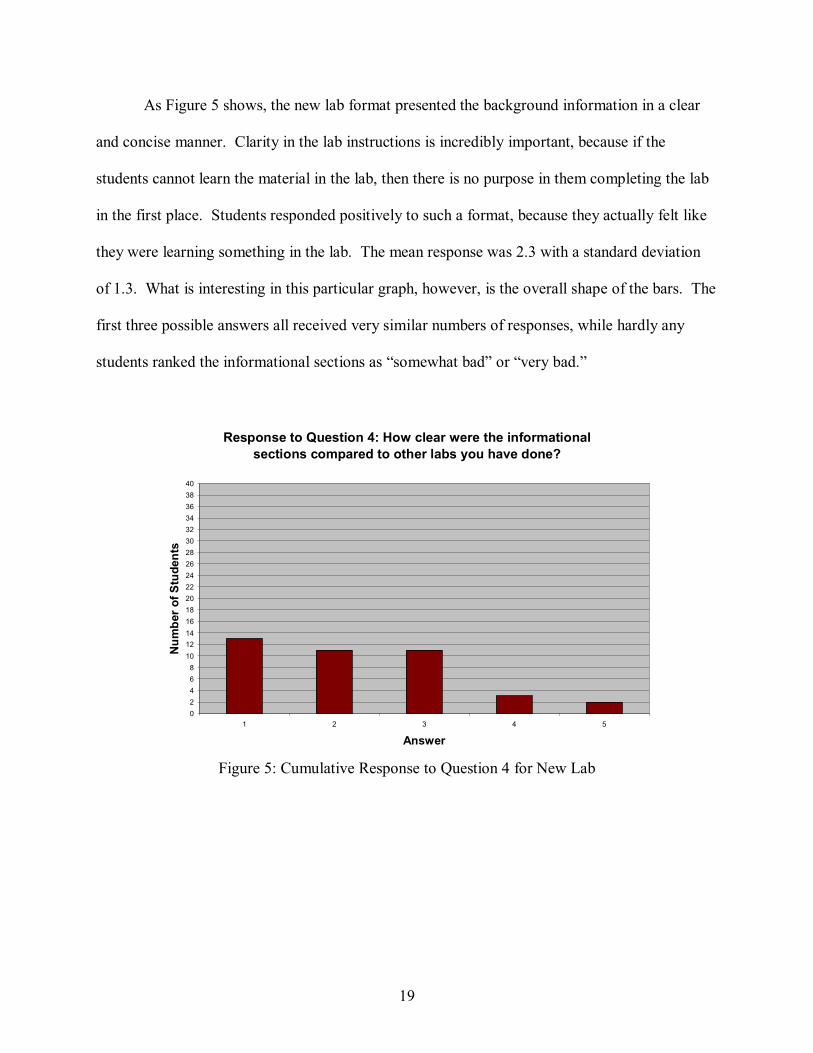
As Figure 5 shows, the new lab format presented the background information in a clear
and concise manner. Clarity in the lab instructions is incredibly important, because if the
students cannot learn the material in the lab, then there is no purpose in them completing the lab
in the first place. Students responded positively to such a format, because they actually felt like
they were learning something in the lab. The mean response was 2.3 with a standard deviation
of 1.3. What is interesting in this particular graph, however, is the overall shape of the bars. The
first three possible answers all received very similar numbers of responses, while hardly any
students ranked the informational sections as “somewhat bad” or “very bad.”
Response to Question 4: How clear were the informational
sections compared to other labs you have done?
0
2
4
6
8
10
12
14
16
18
20
22
24
26
28
30
32
34
36
38
40
1 2 3 4 5
Answer
Nu
mb
er
of
Stu
den
ts
Figure 5: Cumulative Response to Question 4 for New Lab

20
Figure 6 shows the most widely dispersed range of answers to the question of the
effectiveness of the data and analysis sections. A number of students who came to the tests of
the new labs, much to our surprise, expressed dismay at the thought of no lab report; they,
surprisingly enough, find reports to be helpful, useful, and beneficial. We knew when we started
this project that not every student would necessarily be thrilled by the changes we made to the
labs. However, a great many students (30 in total, or 75%) expressed positive sentiments about
our newly designed data and analysis sections, where the data is recorded and calculations made
there in the lab rather than outside after completion of the lab. The mean response was 2.3, with
a standard deviation of 1.3. Even with the naysayers, a great many students were pleased with
the changes in the lab manual, particularly the absence of a lab report for this lab.
Response to Question 5: How effective were the data and
analysis sections in aiding your understanding of the
material?
0
2
4
6
8
10
12
14
16
18
20
22
24
26
28
30
32
34
36
38
40
1 2 3 4 5
Answer
Nu
mb
er
of
Stu
de
nts
Figure 6: Cumulative Response for Question 5 for New Lab
21
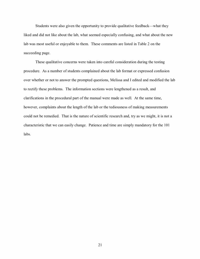
Students were also given the opportunity to provide qualitative feedback—what they
liked and did not like about the lab, what seemed especially confusing, and what about the new
lab was most useful or enjoyable to them. These comments are listed in Table 2 on the
succeeding page.
These qualitative concerns were taken into careful consideration during the testing
procedure. As a number of students complained about the lab format or expressed confusion
over whether or not to answer the prompted questions, Melissa and I edited and modified the lab
to rectify these problems. The information sections were lengthened as a result, and
clarifications in the procedural part of the manual were made as well. At the same time,
however, complaints about the length of the lab or the tediousness of making measurements
could not be remedied. That is the nature of scientific research and, try as we might, it is not a
characteristic that we can easily change. Patience and time are simply mandatory for the 101
labs.
22
.
Problems Positive feedback
Too long 3 Procedure clear
Slow movement in the explosion, rubber band Fill in sections were helpful and clear 4
Placement of the analysis directions confusing 5 Style aided comprehension 2
Need a definition of momentum 3 Ruler track is helpful
Ruler track hard for only two people Concept questions aid understanding 2
Conservation question confusing Information sections were helpful
Need to reference formulas in analysis section
Trial 2
Too long 10 Easy to understand
Analysis is repetitive/Measurement is tedious 2 Concept questions aid understanding 4
Do not like concept questions 2 Fill in sections were helpful and clear 2
Need better instruction for inelastic analysis Liked use of rubber band
Need a definition of momentum Style aided comprehension 3
Prefer a lab report Information sections were helpful
Layout is bad
Trial 3
Analysis is repetitive /Measurement is tedious 9 The procedures are clear 4
Too long 4 Easy to understand 2
Need more time to think for concept questions 2 Concept question aid understanding 3
Did not like analysis/conclusion questions Fill in sections were helpful and clear 5
Informational sections were helpful 2
Style aided comprehension 4
Table 2: Qualitative Responses to Survey for New Lab 7
23
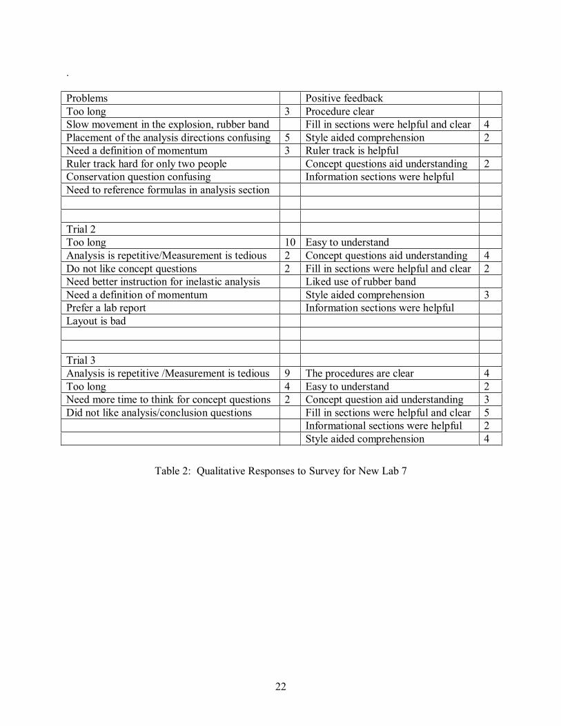
To serve as a basis of comparison, students in the Physics 101 class were asked to fill out
a survey about the original Lab 7 the week after they turned in that lab report. We felt these
surveys were necessary to give us a better understanding of how successful our new lab format
was. In total, 78 students filled out the survey, but not every student, for uncertain reasons,
answered every question. The total number of respondents for each question ranged from 74 to
78 students. These results are displayed in Table 3.
Q 1 Q 2 Q 3 Q 4 Q 5
Score
Number Respon-dents Score
Number Respon-dents Score
Number Respon-dents Score
Number Respon-dents Score
Number Respon-dents
1 8 1 18 1 9 1 8 1 12
2 28 2 35 2 21 2 21 2 23
3 30 3 8 3 33 3 33 3 25
4 10 4 13 4 8 4 9 4 13
5 0 5 0 5 7 5 4 5 2
Table 3: Collected Data from Surveys for Original Lab 7
Overall, the original lab was favored much less than the redesigned one. The mean
number of students who rated this lab in the top two categories was 37, which was roughly 47%
of the polled group. Ten more students ranked this lab more favorably than they had the
redesigned one, but the percentage of students who did so was far less than the 65% in our
redesigned lab. The mean responses tended to lean much closer to the “neutral” range in the
original lab, whereas in the redesigned labs the averages were closer to the “good” range. What
initially surprised us was how many students seemed relatively satisfied with the original lab,
which we thought was overall ineffective and inferior to the other labs in the manual, not to

24
mention our redesigned one. However, students still preferred the new and improved lab to the
one currently used in class.
The results of Question 1 for the original lab are shown in Figure 7. The mean response
was 2.6, and the standard deviation was 1.2. More students were displeased with (or at the very
least more neutral towards) the original lab format than with the redesigned one. Some students
found the measurement process tedious and did not favor the separation of the informational
sections from the procedural instructions. Others, however, felt the layout of the lab was good
relative to others they have performed. Still, the shape of the graph is a sort of bell-curve, in
contrast to the earlier figures for the new lab, which displayed a majority of the responses in the
first two categories.
Answers to Question 1: How was the layout of this lab
compared to other labs you have done?
0
10
20
30
40
50
60
70
80
1 2 3 4 5
Answer
Nu
mb
er
of
Re
sp
on
se
s
Figure 7: Control Group Response to Question 1 for Original Lab

25
Surprisingly, a great deal of students felt that the procedures in the original lab were
clear, as the results in Figure 8 show. The mean response was 2.2 with a standard deviation of
1.0. What is important to note, however, is how varied the responses were. A good number of
students thought the procedures were very clear, while at the same time a good number believed
them to be fairly vague. The new lab did not cause this same level of dichotomy in responses,
and indeed appeared to have provided overall clear and comprehensible procedures for the
majority of students. That, after all, was the point of this research project—to clarify the
procedures and goals of the lab so that the average student could perform well in the educational
environment.
Answers to Question 2: How clear were the procedures?
0
10
20
30
40
50
60
70
80
1 2 3 4 5
Answers
Nu
mb
er
of
Re
sp
on
se
s
Figure 8: Control Group Response to Question 2 for Original Lab

26
Figure 9, which graphically depicts the results of Question 3 for the original lab,
continues the bell-curve trend alluded to in Figure 7. The mean answer was 2.8 with a standard
deviation of 1.0. For the most part, the students were neutral in their feelings about the order of
information in the lab—no one thought it spectacular, but no one really hated it either. In
general, this lack of enthusiasm in either direction signifies a great underlying problem in the
labs. They do not encourage a positive student response or level of enthusiasm. The order of
information needs to be presented in a way that ensures students comprehend the lab itself and
the material it is supposed to teach them. When almost 60% of students surveyed express that
this is not the case, there must be a problem with the lab itself.
Answers to Question 3: How did the order that the information
was presented in aid your understanding of the lab?
0
10
20
30
40
50
60
70
80
1 2 3 4 5
Answers
Nu
mb
er
of
Re
sp
on
se
s
Figure 9: Control Group Response to Question 3 for Original Lab

27
The graph of results to Question 4, shown in Figure 10, continues the aforementioned
bell-curve trend in a much more pronounced manner than any of the previous graphs. The
students appeared to be much more neutral to this lab, and the numbers showed this as well. The
mean was 2.7 with a standard deviation of 1.0. The students were not particularly impressed
with the original lab’s information sections, but neither were they disappointed or frustrated
either. This implies that the original lab’s information sections were on par with the average
level of clarity in the lab manual. Regardless of how clear this average level is, the information
sections definitely need to be improved so that more students feel more favorable to them, as
they did in the redesigned lab. Students should not have to question the informational sections or
the material presented therein. They must be able to comprehend what is being presented in
order to execute the lab and further their knowledge of the material.
Answers to Question 4: How clear were the informational sections
compared to other labs you have done?
0
10
20
30
40
50
60
70
80
1 2 3 4 5
Answers
Nu
mb
er
of
Resp
on
ses
Figure 10: Control Group Response to Question 4 for Original Lab

28
Figure 11 below graphically depicts the student response to Question 5 for the original
lab. As before, this curve has a distinct bell-curve shape, albeit one favoring the positive end of
the spectrum. The results to this question were surprising. I did not feel that the original data
and analysis sections were effective or helpful in any manner. However, the mean student
response was 2.6, with a standard deviation of 1.0. Students evidently believed that these data
sections were helpful in comprehending the presented material. Still, students who participated
in the test of the redesigned lab favored those new data sections more, providing further
implication of the superiority of the new lab format.
Answers to Question 5: How effective were the data and
analysis sections in aiding your understanding of the
material?
0
10
20
30
40
50
60
70
80
1 2 3 4 5
Answer
Nu
mb
er
of
Re
sp
on
se
s
Figure 11: Control Group Response for Question 5 for Original Lab

29
As in the other survey, students were encouraged to provide qualitative feedback and
observations on the original lab. The responses are listed below in Table 4. Many students
testified that they felt the measurements on the air table were tedious and overly time-
consuming. Students also found that the procedural and informational sections are confusing. If
they cannot understand the material or what they are supposed to do, there is no way they will be
able to further their physical knowledge. A significant number also admitted that the lab report
was not an effective educational tool and that they did not understand its purpose. All of the
above demonstrate a massive overall problem with the lab manual—students must understand
why they are performing the labs and why the material is pertinent to their education in physics.
Otherwise, the execution of these labs is futile for the students.
Table 4: Qualitative Survey Results from Original Lab 7
Control
Data analysis procedure was confusing 12 Procedures are clear 4
Analysis is repetitive/Measurement is tedious 33 Analysis questions were clear 3
Need data studio directions 2 Informational sections were clear 2
Lab report is not helpful/ purpose unclear 13
Difficult to align pucks for collision 3
Informational section are unclear 15
Air table is hard to use 2
Style/format was confusing/complicated 5

30
In the control group’s survey, an additional question, as noted before, asked them to
estimate the time they spent working on the lab report. We wanted to see how much time, in and
out of lab, they were spending on research or the understanding of it, and we also wanted to
know if they thought lab reports were an effective use of their time. The results are displayed in
Table 5 below, and the results for time spent on the report are graphically displayed in Figure 12
on the next page.
Time in lab
Time on Report
Effective use of time?
Hours
Number Respon-dents Hours
Number Respon-dents Answer
Number Respon-dents
1 15 1 3 Yes 20
1.5 22 2 22 No 40
2 22 3 22
3 0 4 9
4 0 5 3
5 0 6 0
7 0
8 2
Table 5: Collected Data about Time Concerns from Original Lab 7

31
Time Spent on Lab Report
0
5
10
15
20
25
1 2 3 4 5 6 7 8
Number of Hours
Nu
mb
er
of
Re
sp
on
ses
Figure 12: Number of Hours Spent on Lab Report for Original Lab
As Figure 12 above demonstrates, a vast majority (over 70%) of students spent at least an
additional two hours working on the lab report; this does not include any time spent in lab
performing the experiment itself. The mean amount of time spent was 3.0 hours, with a standard
deviation of 1.3. Of the 61 students that responded to the question of effective use of time, 40
responded that they did not feel that it was. Almost two-thirds of the students did not believe the
lab reports were effective educational tools, in large part because they consumed so much of
their time. This correlates with our research that lab reports, a form of passive learning, are not
as effective as the active and hands-on learning that labs themselves stimulate.
What should be noted is the nature of the test group. Because Professors Chaloupka and
Armstrong provided a small amount of extra credit to those students who participated in our
study, I am afraid we may have received a polarized group of students: those grade-focused with
a strong interest in science and physics already versus those who are struggling to get by and
desperate for help anywhere they can get it. Although the extreme tendencies of both groups

32
would neutralize the other, I would have liked to test the “average” student as well, since this is
the student toward which this project is pointed. Again, this is a hypothesis as to the nature of
the group, but it would explain the desire by some students to have a lab report, since those
already science-oriented would prefer to continue with what they already know.
Lab 8
As with the redesigned Lab 7, we also tested the refined Lab 8. Because of time
constraints and room availability, the lab was only tested once instead of the three trials for Lab
7. Furthermore, this lab was never compared to the original Lab 8 in the manual, in large part
because students completed Lab 8 so long ago that any answers would be inaccurate and unfair
to use. The survey was the same used in the previous lab tests. Five questions with quantitative
answers were posed, and then students were given the opportunity to make qualitative comments
and suggestions. The results of this survey are displayed in Table 6.
Q 1 Q 2 Q 3 Q 4 Q 5
Score
Number Respon-dents Score
Number Respon-dents Score
Number Respon-dents Score
Number Respon-dents Score
Number Respon-dents
1 2 1 5 1 5 1 6 1 5
2 7 2 6 2 6 2 5 2 7
3 5 3 3 3 2 3 3 3 1
4 0 4 0 4 1 4 0 4 1
5 0 5 0 5 0 5 0 5 0
Table 6: Collected Data from New Lab 8
In total, fourteen students tested the new Lab 8 and completed surveys. Although is an
admittedly small group of students, it is still a fairly accurate statement of the effectiveness and
overall student sentiment toward this new lab. On average, 11 students, or 77% of the test pool,

33
ranked the lab as either good or very good. This high of a percentage, even with such a small
group of test subjects, is a remarkable statement on the effectiveness and educational fortitude of
this redesigned lab.
As Figure 13 demonstrates, students responded favorably to the layout of this redesigned
lab. The mean response was 2.2, with a standard deviation of 0.5. This low level of variance
demonstrates that students were remarkably similar in their positive attitudes toward the
organizational layout of the lab. Students appreciated the Data Studio instructions woven into
the lab itself, which prevented them from having to flip through lab manuals hunting for
directions on how to use the computer program. They commented that this lab was more
student-friendly than others they had worked with and appreciated that the layout did not require
them to make large leaps in assumptions or proofs to understand the material being presented.
Question 1: How was the layout of this lab compared to other
labs you have done?
0
1
2
3
4
5
6
7
8
9
10
11
12
13
14
15
1 2 3 4 5
Answer
Stu
den
t R
esp
on
se
Figure 13: Cumulative Response to Question 1 for New Lab 8
34
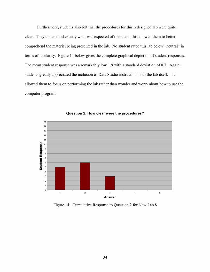
Furthermore, students also felt that the procedures for this redesigned lab were quite
clear. They understood exactly what was expected of them, and this allowed them to better
comprehend the material being presented in the lab. No student rated this lab below “neutral” in
terms of its clarity. Figure 14 below gives the complete graphical depiction of student responses.
The mean student response was a remarkably low 1.9 with a standard deviation of 0.7. Again,
students greatly appreciated the inclusion of Data Studio instructions into the lab itself. It
allowed them to focus on performing the lab rather than wonder and worry about how to use the
computer program.
Question 2: How clear were the procedures?
0
1
2
3
4
5
6
7
8
9
10
11
12
13
14
15
1 2 3 4 5
Answer
Stu
den
t R
esp
on
se
Figure 14: Cumulative Response to Question 2 for New Lab 8

35
Students also responded positively to the order of information in the lab. As Figure 15
shows, 11 of the 14 students, or just under 80% of the group, felt that the order of information
was presented in a “somewhat good” or “very good” manner. Indeed, the average student
response was a low 1.9 with a standard deviation of 0.9. A vast majority of students liked that
the informational sections about rotational and translational motion were separated because it
allowed them to focus on one at a time and not get confused along the way. By first explaining
kinetic and potential energy, and then explicating the difference between what happens in
translational motion and later rotational motion, students were better able to comprehend what
was happening as objects moved down the track.
Question 3: How did the order that the information was
presented in aid your understanding of the lab?
0
1
2
3
4
5
6
7
8
9
10
11
12
13
14
15
1 2 3 4 5
Answer
Stu
den
t R
esp
on
se
Figure 15: Cumulative Response to Question 3 for New Lab 8

36
The student response was again quite positive in the area of clarity of informational
sections. Like had happened in Questions 1 and 2, virtually no one gave this question a lower
ranking than “neutral.” The mean response, as Figure 16 demonstrates, was a low 1.8 with a
standard deviation of 0.8. Indeed, the bell-curve shaped graphs like those in the results of the
original Lab 7 tests are not existent in these evaluations. Eleven of the 14 surveyed students, or
just under 80% of the students surveyed, felt that the level of clarity was good or very good.
This result, I believe, is a testament of the clear and explicit development of equations; even
relatively simple rearrangements were produced on paper to ensure that students followed every
step of the process. Such well-developed and thorough informational sections allowed students
to better absorb the material before they performed the lab so that they could better understand
the results after they produced them.
Question 4: How clear were the informational sections
compared to other labs you have done?
0
1
2
3
4
5
6
7
8
9
10
11
12
13
14
15
1 2 3 4 5
Answer
Stu
den
t R
esp
on
se
Figure 16: Cumulative Response to Question 4 for New Lab 8

37
Students, as Figure 17 shows, greatly appreciated the data and analysis sections of the
new Lab 8. The mean student response was 1.9 with a standard deviation of 0.8. Over 85% of
the students surveyed, or 12 of the 14 individuals, considered the data and analysis sections to be
“somewhat good” or “very good.” Unlike in the redesigned Lab 7, students were still required to
compose a lab report. However, the spaces provided for the recording of data, including constant
measurements, and performing calculations allowed students to perform much of the analysis in
the lab itself. Therefore, any questions that may develop later could be answered by the TA
immediately rather than struggled over while the report was being written. Furthermore, these
spaces ensured that students would not overlook making a measurement or mistakenly record it
elsewhere. Having all data in a centralized location decreased the chance of external
complications affecting analysis.
Question 5: How effective were the data and analysis sections
and conceptual questions in aiding your understanding of the
material?
0
1
2
3
4
5
6
7
8
9
10
11
12
13
14
15
1 2 3 4 5
Answer
Stu
de
nt
Resp
on
se
Figure 17: Cumulative Response to Question 5 for New Lab 8
38
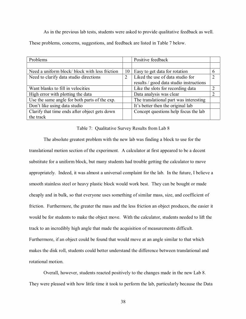
As in the previous lab tests, students were asked to provide qualitative feedback as well.
These problems, concerns, suggestions, and feedback are listed in Table 7 below.
Problems Positive feedback
Need a uniform block/ block with less friction 10 Easy to get data for rotation 6
Need to clarify data studio directions 2 Liked the use of data studio for
results / good data studio instructions
2
Want blanks to fill in velocities Like the slots for recording data 2
High error with plotting the data Data analysis was clear 2
Use the same angle for both parts of the exp. The translational part was interesting
Don’t like using data studio It’s better then the original lab
Clarify that time ends after object gets down
the track
Concept questions help focus the lab
Table 7: Qualitative Survey Results from Lab 8
The absolute greatest problem with the new lab was finding a block to use for the
translational motion section of the experiment. A calculator at first appeared to be a decent
substitute for a uniform block, but many students had trouble getting the calculator to move
appropriately. Indeed, it was almost a universal complaint for the lab. In the future, I believe a
smooth stainless steel or heavy plastic block would work best. They can be bought or made
cheaply and in bulk, so that everyone uses something of similar mass, size, and coefficient of
friction. Furthermore, the greater the mass and the less friction an object produces, the easier it
would be for students to make the object move. With the calculator, students needed to lift the
track to an incredibly high angle that made the acquisition of measurements difficult.
Furthermore, if an object could be found that would move at an angle similar to that which
makes the disk roll, students could better understand the difference between translational and
rotational motion.
Overall, however, students reacted positively to the changes made in the new Lab 8.
They were pleased with how little time it took to perform the lab, particularly because the Data

39
Studio instructions were explicitly detailed in the lab itself. They thought this new lab was more
effective at teaching the material and that Data Studio now helped analyze the material for
comprehension rather than serve as a hindrance in its performance, as it had done so previously.
Ultimately, this new lab was a more effective educational tool than its original counterpart.
Final Thoughts
Overall, I believe this senior research project accomplished what Melissa and I set out to
do. We designed four new labs that will improve the effectiveness of the education of the
Physics 101 Labs. Moreover, I believe we have set a precedent for improvement of the lab
program in general. I am not so naïve to think that every suggestion or revision that we have
made will be implemented in the future. What I would like to believe, however, is that we have
shown through the course of this project that reports are not absolutely essential to the learning
process, that students should be encouraged to learn and understand the material in the laboratory
rather than in their dorm rooms, and that advanced technology can improve the quality of lab
instruction.

Appendix A
Lab Manual
40
Introduction to Physics 101 Labs
The study of physics looks for an explanation to everything in the world—why planets
circle the sun, why everything falls with the same acceleration on earth, why negative charges
attract positive ones. Like many other phenomenon, there is a simple explanation why you are
all enrolled in Physics 101L: because the department forces you. It is impossible to understand
physics, even at the most basic level, without any sort of hands-on experimentation. Because
what you are to learn this semester is so fundamental to the study of physics—and, indeed, the
study of science itself—it is pertinent that you fully comprehend the presented material. In order
to ensure this complete and total comprehension, one must perform labs as well as attend class.
This year, in both lab and lecture, you will learn a number of important and invaluable
physical concepts and theories, information that men and women have devoted their lives to
determining. We cannot promise that you will remember every detail of every lecture, or that
you will be able to recall a single lab you will have performed in five years. What we hope you
take out of this class and lecture, rather, is a better understanding of the scientific process and
scientific inquiry. For those of you interested in a career in science, this will undoubtedly prove
a vital, necessary, and fundamental tool. For those of you who will not embark on such a career
path (including, truth be told, one of the editors of this manual), there is still much to learn in this
lab. You cannot read a newspaper today without some reference to science or technology. Nor
can you perform a logic puzzle without utilizing the basic analytical tools you will develop and
refine in the labs to come. In order to function as an educated member of today’s society, you
must develop, grasp, and show a keen sense of analysis, logical processing, and scientific
thought. These Physics 101 Labs, then, are not merely an introduction to physics but also an
introductory class in how to be a responsible human being.

Appendix A
Lab Manual
41
Name
Lab Partner: Their Name
Lab Section
Date
Lab #: Title
Purpose: In this section, you discuss the motivation of this lab and detail any relevant
background information to the lab, such as laws, equations, or unit analysis. The main idea is to
discuss why this lab is important and necessary in furthering your education of physics. A
typical purpose statement is a short paragraph.
Procedure: In a clear, organized manner you will briefly summarize the steps of the lab. This
section should not be a word-for-word copying from the lab manual itself. It is your
responsibility here to note what you did, how you did it, and what equipment was utilized. The
language should be clear and concise, so that someone outside of the lab could understand what
you did and replicate it if needed.
Data and Analysis: In this section you record all raw data you collected using graphs, data
tables, and any equations provided either in the lab itself or in lecture. It is pertinent that you
show your calculations in this section so that others may know exactly how you obtained your
conclusions. Do not exclude any data, even if you feel that it is a source of error. Include it,
demonstrate the error (if possible), and explain why the error exists. It could be a malfunction of
the equipment, for instance, or simple human error in making precise calculations. Furthermore,
discuss any uncertainties, surprises, problems, or concerns that arose during the lab itself, and
how these could be avoided or resolved in the future.

Appendix A
Lab Manual
42
It is imperative that this section is technically sound. Therefore, include all calculations
and use the correct units. If necessary, perform dimensional analysis to demonstrate how your
units were determined. Furthermore, label every graph, figure, and equation with an identifying
number, and be certain to title your graphs and label your axes. Any time a figure is introduced,
be it a graph, data table, or illustration, be sure to follow it up with an explanation of its
importance to the lab and/or the analysis of it, as well as any conclusions that may be drawn
from it.
Conclusions and Error Analysis: At the end of the lab, you have the opportunity to discuss
whether or not the lab confirmed both the law being tested and your hypothesis of it.
Furthermore, you also must perform error analysis to demonstrate how closely your performance
of the lab was consistent with what the theory predicted. For more on error analysis, please see
Lab 1.
Experimental science is different from many other disciplines in that there need not
always be a “correct” answer. Nor must one discover said right answer to learn from the
experiment. If you do not achieve the correct answer, do not give up and deem your lab a
failure. Instead, look to reasons and explanations for why you did not achieve what you had
hoped to. Was the equipment faulty? Were incorrect, or incorrectly performed, equations
utilized? Was the procedure followed exactly, or were mistakes made in the execution of the lab
itself? Is the theory, in fact, correct? So long as you search out an explanation for the reasons
why your lab was not perfect, it was not a failure performed in vain.
Appendix A
Lab Manual
43
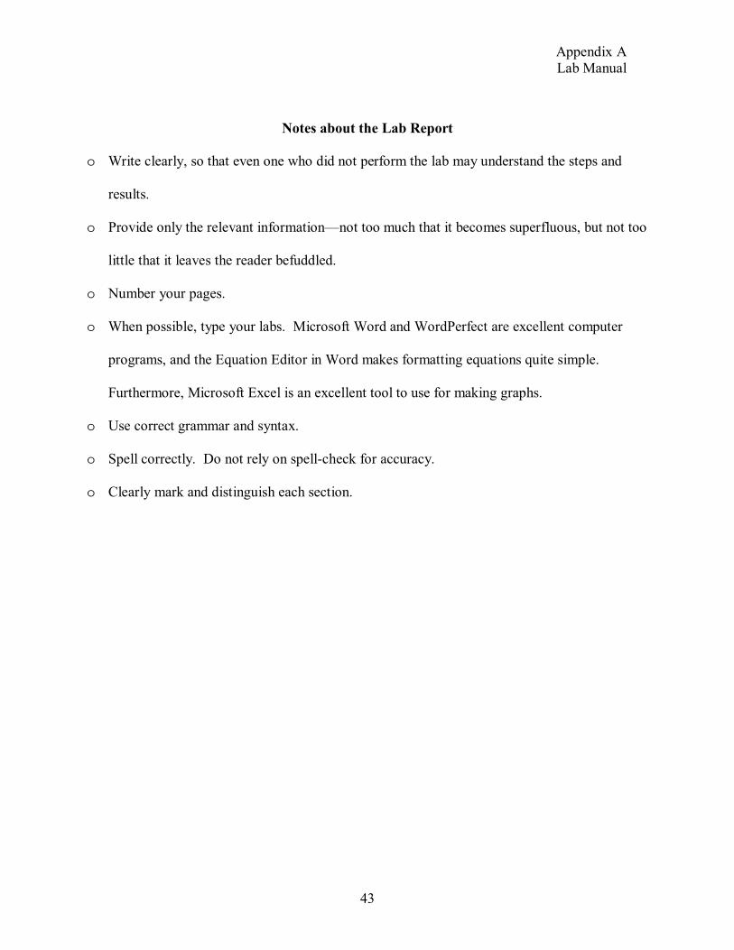
Notes about the Lab Report
o Write clearly, so that even one who did not perform the lab may understand the steps and
results.
o Provide only the relevant information—not too much that it becomes superfluous, but not too
little that it leaves the reader befuddled.
o Number your pages.
o When possible, type your labs. Microsoft Word and WordPerfect are excellent computer
programs, and the Equation Editor in Word makes formatting equations quite simple.
Furthermore, Microsoft Excel is an excellent tool to use for making graphs.
o Use correct grammar and syntax.
o Spell correctly. Do not rely on spell-check for accuracy.
o Clearly mark and distinguish each section.

Appendix A
Lab Manual
44
Microsoft Excel How-To
Microsoft Excel is a powerful tool, especially in the physics lab. It allows for the
collection and organization of data, as well as the construction and production of graphs. As
with many tools, however, the software is only useful if you understand to use it. The following
instructions on creating graphs in Microsoft Excel should not be considered to be extensive or
all-encompassing. Rather, they are intended to provide a skeletal framework from which you
can develop your own experience and familiarity with the program.
o Type or input your data into the columns provided in one of the worksheets in Excel. Make
sure you keep the different variables in separate columns so as not to negatively affect your
results.
o Hint: Once you get more skilled using Excel, you may also use it to help with your
calculations rather than doing them by hand or calculator.
o Highlight the columns of data that you would like to graph, and then click on the Chart
Wizard icon on the toolbar. The Chart Wizard icon has a red, blue, and yellow graph of
columns displayed on it.
o Select the type of graph you would like under the Column Types tab. For line graphs, select
the “X-Y Scatter” option. To determine if your data results make physical sense, you may
select the “Press and Hold to View Sample” button to view the graph of the data.
o Note: This graph may appear tilted or cockeyed if what you have wanted to be the x-
and y-values have been reversed by the software.
o Hit “Next,” and you will be sent to the Source Data window. To change which values are on
which axis, press the button with the red arrow to the right of the “X Values” or “Y Values”

Appendix A
Lab Manual
45
box. To select the data for that particular axis, highlight it with the box with the flashing
dotted line. The “Next” button will bring you to the Chart Options window.
o Note: If at any time you want to undo an action in a previous window, select the
“Back” button.
o In the Chart Options window, under the Titles tab, you may label the axes and the graph
itself. Make sure to include any relevant units in the labels. Under the Gridlines tab, you
may show or delete the gridlines as you desire. Lastly, the Legend tab will allow you to hide
the graph’s legend if you so desire.
o Click “Next,” and you will be sent to your last window, which will allow you to determine
where you would prefer to place the new graph. You can choose to store it on the sheet in
which your data is stored, or you may create an entirely new sheet solely for the graph. That
is entirely up to your discretion. Then click “Finish.”
o To change the color of the plot area, double click any part in the background of the graph and
select which color you would prefer.
o To create a line of best fit, right-click on one of the data points. An Add Trendline window
will appear, and you can decide which kind of line you would like the line of best fit to be.
Clicking the Options tab, you can choose to display the equation for this line on the graph.
This is at your discretion, but it may prove helpful in later calculations, especially if you will
need to differentiate or integrate at any time during these calculations.

Appendix A
Lab Manual
46
3 MOTION WITH CONSTANT ACCELERATION
Purpose:
Study and understand how objects move under constant acceleration in one and two directions.
3.1 List of Equipment:
• Ball
• High speed camera
3.2 Motion with Constant Acceleration: One Dimension
Lab 2 showed that the motion of objects in free fall can be described by the kinematics
equations:
tavv yyy +=0
(1)
)(2 0
22
0yyavv yyy −+= (2)
2
02
10
tatvyy yy ++= (3)
where y is the position of the object at the time, t, 0y is the initial position of the object at t = 0,
yv is the velocity of the object at the time, t,0yv is the initial velocity of the object, and ya is the
objects acceleration.
Free fall is a term for objects that are moving with constant acceleration due to the force
of gravity. Free fall is a special case of motion with constant acceleration, but the kinematics equations used to describe free fall motion also describe the motion of any object under constant
acceleration. This includes objects moving in one, two, or even three dimensions.
Observing motion with constant acceleration is common in daily life. A ball that has been tossed straight up in the air is an example of motion with constant acceleration one
dimension. (Figure 1) When tossing a ball, the toss gives it an initial force upward (in the
positive y direction) which means that it has an initial velocity, yvv =0 , in that direction.

Appendix A Lab Manual
47
The ball, like the free fall object in Lab 2, also has a constant acceleration due to gravity. The
deceleration due to gravity causes the ball’s upward (y direction) velocity to become slower and slower until it has a velocity, vy = 0. At this point the ball falls just like an object in free fall.
Q 1. What is the acceleration of the ball when it reaches its highest point?
Q 2. What is it’s velocity at the highest point?
3.3 Motion with Constant Acceleration: Two Dimensions
Similar to the ball that is tossed straight up, a ball that is thrown is an example of motion
with constant acceleration in two dimensions. (Figure 2) The throw gives the ball an initial force upward (in the positive y direction) as well as a force outward (in the positive x direction), so the
ball has an initial velocity, 0v , with components in both directions vx and vy.
vy
vy =0
vy
vy = v0
t = 0 t = ½ total t > ½ total
Figure 1

Appendix A Lab Manual
48
Q 3. How does the acceleration in the x-direction affect the path of the ball?
The initial velocity in each direction can be found by breaking the initial velocity vector down into its horizontal and vertical components. (Figure 3)
v
v
v
v = vx
vy =0
v0
t = 0 t = ½ total t = total
Figure 2
v0 vy
vx
v0vy
vx
Figure 3
Appendix A Lab Manual
49
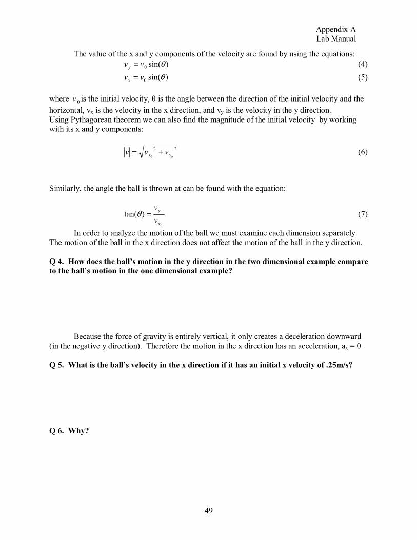
The value of the x and y components of the velocity are found by using the equations:
)sin(0 θvv y = (4)
)sin(0 θvvx = (5)
where 0v is the initial velocity, is the angle between the direction of the initial velocity and the
horizontal, vx is the velocity in the x direction, and vy is the velocity in the y direction.
Using Pythagorean theorem we can also find the magnitude of the initial velocity by working with its x and y components:
22
0 oyx vvv += (6)
Similarly, the angle the ball is thrown at can be found with the equation:
0
0)tan(x
y
v
v=θ (7)
In order to analyze the motion of the ball we must examine each dimension separately.
The motion of the ball in the x direction does not affect the motion of the ball in the y direction.
Q 4. How does the ball’s motion in the y direction in the two dimensional example compare
to the ball’s motion in the one dimensional example?
Because the force of gravity is entirely vertical, it only creates a deceleration downward (in the negative y direction). Therefore the motion in the x direction has an acceleration, ax = 0.
Q 5. What is the ball’s velocity in the x direction if it has an initial x velocity of .25m/s?
Q 6. Why?

Appendix A Lab Manual
50
3.4 Procedure
• Follow your lab TA’s instruction on how to take an extended exposure photo of you and
your partner throwing a ball to one another. (For the best results throw the ball high into the air to get a longer arc. This will provide you with more points for analysis)
• Open the Kinematics Manipulations program on your computer.
• Import your photo into the program.
• Open the photo in the program window and click on each point in the photo where you see the ball, beginning with the first point you see after the ball left the thrower’s hands
• Create the scale in meters using the tool in the toolbar.
• Create a best fit line for the ball’s path using the regression tool in the toolbar
3.5 Analysis
• Use the Kinematics Manipulations program to find the ball’s initial velocity, 0v and the
initial angle of the throw, .
• Start by finding the initial velocity in the x and y directions, 0xv , and
0yv .
o Hint: You can find the ball’s highest point by finding the maximum of the best fit line using the tool in the toolbar.
• Choose the equation you want to use by clicking on it.
• Rearrange the equation by clicking on the variable you want to solve for.
• Make sure to enter all the pertinent information you know in the boxes next to the variables and press solve.
• Use the components of velocity in equations (6) and (7) to find the ball’s initial velocity,
0v and the initial angle of the throw, .
3.6 Conclusions
Q 7. How does the velocity and angle calculated compare with your expectation of the
values based on looking at the photo?
Q 8. Explain any errors that may have occurred.

Appendix A Lab Manual
51
Lab 3 Program Requirements and Sample Run-Through
Purpose: students take a picture of a ball being thrown and use the points along the trajectory to
find the initial velocity, v0.
The computer program will allow a student user to import a digital photo as input. This
photo will be displayed on the monitor, as seen in Figure 1.
Figure 1: Photo of Ball Trajectory
There will be a toolbar where the user can choose a pointer that will allow her to pick a
point on the image by clicking on the screen. Using this method, the student will select each
point in the image where the ball appears as seen in Figure 2.
Figure 2: Photo of Ball Trajectory with Points

Appendix A Lab Manual
52
This pointer method will also allow a student to erase the point if she is not satisfied with
its placement. The first point, which may be arbitrarily chosen by the student, will be labeled
(0,0).
The program will then ask the user to input distance between two arbitrary selected points
to create a scale. Each point will be labeled using an (x,y) coordinate system after the scale has
been created. If no scale is established, the default scale will be based on the number of pixels in
the image.
Another link on the toolbar will allow the student user to list all chosen points on the
image in a table, with one column being the x-coordinate and another the y-coordinate.
There will also be a function in the toolbar where the student user can create regression
graphs over the ball’s trajectory in the image on the screen. The student user must be able to
choose from a number of regression options, including:
• y = x
• y = x2
• y = x3
• y = x-1
• y = ln x
• y = ex
This way, the student user must decide what type of curve the line of best should be.
When the user chooses a regression type, the line of best fit will be displayed in a graph on the
screen over the digital image of the ball’s trajectory as seen in Figure 3. The student then will be
able to determine the maximum and minimum points on this line along with their coordinated
positions, using a separate tool on the toolbar.

Appendix A Lab Manual
53
Figure 3: Photo of Ball Trajectory with Points and Gridlines
Below the image of the ball’s trajectory on the screen, there will be an equations box that
will list the three kinematics equations:
tavv yyy +=0
(1)
)(2 0
22
0yyavv yyy −+= (2)
2
02
10
tatvyy yy ++= (3)
for the student’s use. The student will select one of the three kinematics equations via a button
next to each equation. The student will then be able to select the “Solve for __” function that
will allow her to see a rearranged version of the equation which has been solved for that variable.
Under the kinematics equations there will be a box which asks:
“What information do we know?
(Hint: choose points we know the most about such as vy = 0.)”
All variables that are part of the kinematics equations will be listed in the box below this
question. Next to each variable will be a location for data input so that the user can type data
values through the keyboard and submit said data into the computer program. The student can
use the “Apply Data” function which will put all known data into the rearranged equation that
they have chosen and then solve it. If the necessary amount of data is not provided, an error
message will appear that will prompt the user to enter more data.

Appendix A Lab Manual
54
This program will be used to solve for the ball’s original velocity and the angle at which
it was originally released. Students will use the kinematics equation function to find the velocity
in for the horizontal component and for the vertical component. Then they will have to use this
data to find v0 and .
Sample Equation work based on the best fit line from the photo in Figures 1-3 as seen in Figure 4
below:
Figure 4: Line of Best Fit for Ball Trajectory
We found the line of best fit of the trajectory of the object to be:
43477.00908.32239.2 2 ++−= xxy (4)
Using this equation, we found the object’s height peaked at the point (0.694930,
1.10867). Using this data and the knowledge that acceleration in the y-direction is simply the
acceleration due to Earth’s gravity, we used the equation:
)(2 00
2
0yyavv yy −+= (5)
The computer program will rearrange this equation to produce:
)(2 0
2
0 yyavv yy −−= (6)
Y-p
ositio
n (m
ete
rs)
Trajectory of Object
-0.4
-0.2
0
0.2
0.4
0.6
0.8
1
1.2
0 0.2 0.4 0.6 0.8 1 1.2 1.4 1.6
X-position (meters)
Appendix A Lab Manual
55
This equation determines that the initial velocity in the y direction of the object, 0yv , is
4.66154 m/s.
To determine the velocity in the x-direction, we first solved for the time it took for the
object to reach its peak. To do this, we used Equation 1 from above. The computer program will
rearrange said equation to solve for t, so that it becomes:
y
yy
a
vvt
)(0
−= (7)
By substituting in values that we know, we determined that the time it took for the object to
reach its peak was t = 0.47567 seconds.
We then used the kinematics equation:
2
02
10
tatvxx xx ++= (8)
to find the initial velocity in the x-direction. Rearranging this equation to solve for the initial
velocity in the x-direction, the computer program would then print out:
t
taxx
vx
x
)2
1( 2
0
0
−−
= (9)
Knowing that the acceleration in the x-direction is zero, and substituting in the other values we
know, we can determine the initial velocity in the x-direction as 1.36502 m/s.
To determine the initial velocity we substitute the values for the initial velocities in the x-
and y-directions into the equations:
22
0 oyx vvv += (10)
0
0tanx
y
v
v=θ (11)
Equation (10) gives the magnitude of the initial velocity as 4.85729m/s and, Equation (11) gives
the initial angle of the throw to be 73.67868o.
Appendix A Lab Manual
56
4 VECTORS AND FORCES
4.1 Purpose: To perform an Exercise in Adding Vectors and Introduce the concept of Forces
4.2 List of Equipment
o Force Tableo Masses
o Balanceo Protractor
o A piece of string 50 centimeters long
4.3 Vectors
A vector is probably the most frequently used entity in physics to characterize space. It can represent the spatial behavior of many things: electric and magnetic fields, fluid flows,
mechanical forces, velocities and accelerations.
For an N dimensional space, a vector is an array of N numbers. For example, a vector representing a point in a plane (N = 2) can be expressed using two quantities: the point’s
distance from an origin, r, and its angle, .
In this lab we will model an N = 2 system having multiple forces. The forces will be such that they add to 0. There will be no system motion because the system is in static
equilibrium.
4.4 The Force Table
The model itself will be a force table. As mentioned above, it will study planar (two-dimensional) force vectors in static equilibrium. The force table consists of a circular metal disk
having a calibrated angular scale. Three masses, mi, are suspended from the disk’s rim with strings. The three strings are tied together at the center of the disk. The masses and/or angular
positions of the strings are adjusted until the three mass + string system is in static equilibrium. See Figure 1.

Appendix A Lab Manual
57
Figure 1: The Force Table
The force acting along the ith string is proportional to the mass hung from that string,
CBAi mm ,,= , since
,gmF i= (1)
where g = 9.8 m/s2. The total force is the vector sum of the three string forces:
= i
tot FF (2)
By varying the masses and the directions of the strings, totF can be adjusted to zero and the
string system will be in static equilibrium. At equilibrium, the ring will be suspended about the
table’s center pin without touching it. The resulting force acting on the ring is:
0=++= CBAtot FFFF (3)
There are two techniques for calculating totF :
1. Calculate the x,y components of the forces
2. Draw vectors representing the three forces and add them using parallelograms. Because of the very basic and unsophisticated nature of this method, this lab will
focus primarily on the first technique.
mC
mB
mA
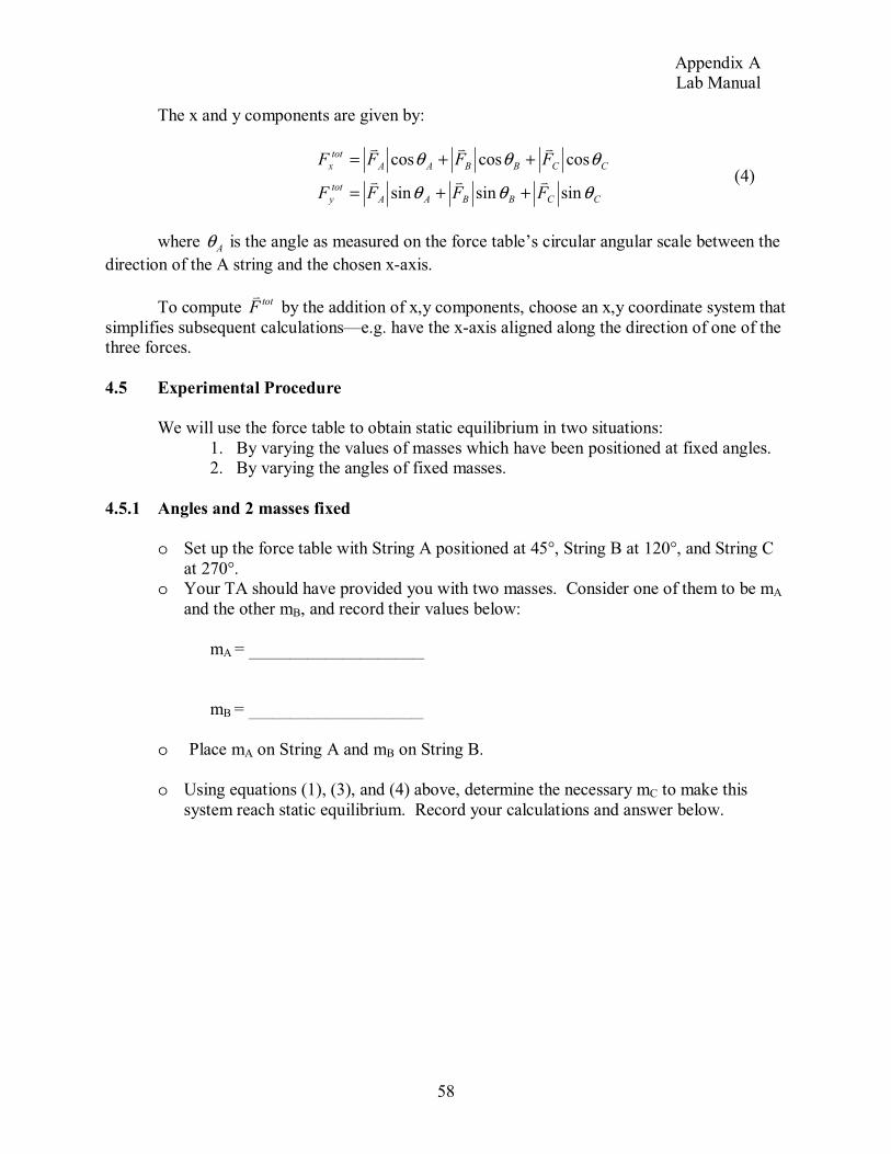
Appendix A Lab Manual
58
The x and y components are given by:
CCBBAA
tot
y
CCBBAA
tot
x
FFFF
FFFF
θθθ
θθθ
sinsinsin
coscoscos
++=
++= (4)
where Aθ is the angle as measured on the force table’s circular angular scale between the
direction of the A string and the chosen x-axis.
To compute totF by the addition of x,y components, choose an x,y coordinate system that
simplifies subsequent calculations—e.g. have the x-axis aligned along the direction of one of the three forces.
4.5 Experimental Procedure
We will use the force table to obtain static equilibrium in two situations:
1. By varying the values of masses which have been positioned at fixed angles. 2. By varying the angles of fixed masses.
4.5.1 Angles and 2 masses fixed
o Set up the force table with String A positioned at 45°, String B at 120°, and String C
at 270°. o Your TA should have provided you with two masses. Consider one of them to be mA
and the other mB, and record their values below:
mA = ______________________________
mB = ______________________________
o Place mA on String A and mB on String B.
o Using equations (1), (3), and (4) above, determine the necessary mC to make this
system reach static equilibrium. Record your calculations and answer below.

Appendix A Lab Manual
59
mC = ____________________
o Check your answer by placing your calculated value for mC at on String C.
Q 1: Is your system at stable equilibrium? If not, what should you have done to reach
static equilibrium?
4.6.2 Masses and 2 angles fixed
o Set up the force table with String A at 120° and String B at 270°.
o Determine a system of masses to use so that CBA mmm 2== . Record your masses
below.
mA = ____________________
mB = _____________________
mC = _____________________
o Using Equations (1), (3), and (4), determine where String C should be to make the system in stable equilibrium.
o Record your calculations and answer below.
String C = __________________
Q 2: Was your result correct? Why or why not?

Appendix A Lab Manual
60
4.6.5 Using Vectors to Problem Solve
Your TA will give you a slip of paper with a starting point and an ending point of two
places in Small. You and your partner will measure the distance between these two points using only the 50 centimeters of string and a protractor. Apply what you learned about the addition of
vectors, making sure to keep careful note of the horizontal and vertical distances as you add them.

Appendix A Lab Manual
61
7 CONSERVATION OF LINEAR MOMENTUM
7.1 Purpose – to demonstrate the principles of conservation of linear momentum
7.2 Equipment
• Air table
• Magnetic pucks
• Rubber band
• Scissors
• Velcro collar
• Lead collar
• Protractor and plastic ruler
• Two yard sticks
7.3 Special Caution
• Do not touch the air table or pucks while the spark timer is on.
7.4 Conservation of Linear Momentum
The total linear momentum, p =mv, in an isolated system always remains constant. An isolated system is a system that doesn’t interact with the rest of the world. This means that the
sum of all the forces on the system arising from the rest of the world is zero. If the system is an isolated group of particles, the total linear momentum of the particles after collisions equals the
total linear momentum from before the collision.
The law of conservation of momentum is useful for determining the motion in the system especially when we do not understand how the internal forces within the system interact. For
example, we can determine the paths, velocities and masses of atoms in a collision even though we do not completely understand the specific nature of inter-atomic forces.
Kinetic energy, unlike linear momentum, may not be conserved even in an isolated
system. Particles’ initial kinetic energy may be expended in heating during the collisions.
Since momentum varies linearly with velocity, momentum conservation yields equations in linear velocity. Kinetic energy on the other hand varies with the square of velocity, so it is
characterized by quadratic equations.
This lab examines several experiments in conservation of momentum by using moving pucks. The sum of all the external forces acting on the puck system is zero and friction is
minimized by using an air table to support the pucks.
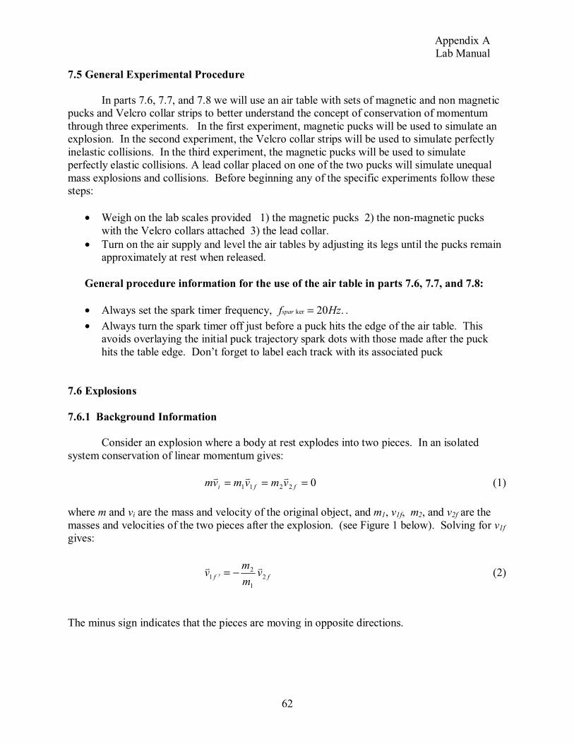
Appendix A Lab Manual
62
7.5 General Experimental Procedure
In parts 7.6, 7.7, and 7.8 we will use an air table with sets of magnetic and non magnetic pucks and Velcro collar strips to better understand the concept of conservation of momentum
through three experiments. In the first experiment, magnetic pucks will be used to simulate an explosion. In the second experiment, the Velcro collar strips will be used to simulate perfectly
inelastic collisions. In the third experiment, the magnetic pucks will be used to simulate perfectly elastic collisions. A lead collar placed on one of the two pucks will simulate unequal
mass explosions and collisions. Before beginning any of the specific experiments follow these steps:
• Weigh on the lab scales provided 1) the magnetic pucks 2) the non-magnetic pucks
with the Velcro collars attached 3) the lead collar.
• Turn on the air supply and level the air tables by adjusting its legs until the pucks remain approximately at rest when released.
General procedure information for the use of the air table in parts 7.6, 7.7, and 7.8:
• Always set the spark timer frequency, .20ker Hzfspar = .
• Always turn the spark timer off just before a puck hits the edge of the air table. This avoids overlaying the initial puck trajectory spark dots with those made after the puck
hits the table edge. Don’t forget to label each track with its associated puck
7.6 Explosions
7.6.1 Background Information
Consider an explosion where a body at rest explodes into two pieces. In an isolated
system conservation of linear momentum gives:
02211 === ffi vmvmvm (1)
where m and vi are the mass and velocity of the original object, and m1, v1f, m2, and v2f are the
masses and velocities of the two pieces after the explosion. (see Figure 1 below). Solving for v1f
gives:
ff vm
mv y 2
1
21 −= (2)
The minus sign indicates that the pieces are moving in opposite directions.

Appendix A Lab Manual
63
Figure 1: Graphical Portrait of an Explosion
Before the explosion the total kinetic energy of the system is zero; however, after the
explosion the system kinetic energy is not zero.
Q 1) Why does the kinetic energy change?
Q 2) Is total energy conserved? Why or why not?
7.6.2 Procedure for Explosion Simulation
• Place a sheet of white paper on to of a graphite sheet on top of the air table.
• Place two magnetic pucks, with the lead collar on one puck, on the white sheet next to each other.
• Place the rubber band around the rims of the two pucks so that they are held together.
• Make sure that the pucks are at rest, then start the sparker and cut the rubber band
m m2
m1v1f
v2f

Appendix A Lab Manual
64
• When the rubber band breaks, the pucks will be repelled from each other. Stop the timer before either puck hits the table edge.
• Label the resulting trajectories and remove the white sheet for analysis.
7.6.3 Analysis of the Puck’s Trajectory
• For each trajectory leg, (e.g. trajectory of puck #2 after collision), measure the inter spark dot spacings, x .
• Find their average x∆ .
• Calculate the puck’s velocity on the trajectory leg, t
xv
∆
∆= , where
.sec20
11
ker
==∆sparf
t
• Using your measured values of the puck masses, calculate the magnitude of the puck’s momentum,
mvp = (3)
and the puck’s kinetic energy,
2
2
1mvKE = (4)
for each leg.
• Using a protractor measure and record the angles of the trajectory legs, with respect to the x-axis.
• Calculate the x and y components of the puck’s momentum, px and py. For example, the
y component of the outgoing momentum of puck #2 equals fff vmvm yy 22222 sinθ= .
7.6.4 Data Collection and Analysis
Note: For ease draw the x-axis along the direction of one of the two outgoing pucks. Use
equations (1) and (2) from the background information to aid in your analysis
Puck #1 x∆ = ______ Puck #2 x∆ = ______
v = ______ v = ______
p = ______ p = ______
KE = ______ KE = ______

Appendix A Lab Manual
65
px = ______ py = ______ px =______ py = ______
Q 3) How well are the before/after x and y momentum components conserved?
Q 4) Explain your results, is this what you expected? Why? Make sure to explain any
discrepancies between your data and your expectation.
Collisions
General Background Information
A collision occurs when projectile collides with a target that is initially at rest.
Conservation of momentum in an isolated system gives:
022111 =+= ffi vmvmvm (5)
There are two unknown vectors on the right hand side, v1f and v2f . Even if v1i is given, we cannot uniquely determine v1f or v2f. To solve for the two unknowns we need to use some
subsidiary condition such as the elasticity, which is the amount of kinetic energy that is conserved, to give us a second equation. A perfectly elastic collision exactly conserves kinetic
energy. A perfectly inelastic collision the colliding bodies stick together and kinetic energy is not conserved.
7.7 Perfectly Inelastic Collisions
7.7.1 Background Information
Let us assume that the collision is perfectly inelastic; the two bodies stick together after
the collision so, fff vvv y == 21 . By conservation of momentum, vf is along the same path as v1i.
This gives:
fi vmmvm )( 2111 += (6)

Appendix A Lab Manual
66
and by rearranging Equation (4) we get:
)( 21
11
mm
vmv i
f+
= (7)
Let us calculate the fractional kinetic energy loss, KE
KE∆ , which is called the inelasticity:
2
1121
2
21
2
1121 ))((
i
fi
i
fi
vm
vmmvm
KE
KEKE
KE
KE +−=
−=
∆ (8)
By substituting Equation (7) we have:
+
−=+
−
=∆
21
1
2
121
21
2
11
2
21
1mm
m
vm
mm
mmv
KE
KE
i
i
(9)
Q 5) If the projectile and target have the same mass, what will the inelasticity be from their
collision?
7.7.2 Procedure for Inelastic Collision Simulation
Equal Masses
• Place a sheet of white paper on top of a graphite sheet.
• Place two non-magnetic pucks, with Velcro collars attached, on the white sheet.
• Place one puck at the center of the table as the target.
• Place a yard stick on either side of the two pucks to create a straight runway for the pucks to travel in. This ensures that the collision is a precise head-on collision.
• With an insulating stick, (to avoid shock), push the projectile puck toward the target puck in a precise head-on collision.

Appendix A Lab Manual
67
• Remove the yard sticks before the collision occurs. If it is a precise head-on collision the pucks should not rotate around one another. You may need practice a few times with the
sparker off to get a correct collision.
• Remove the white sheet for analysis.
Unequal Masses
• Place a fresh sheet of white paper on the air table. Use as a target a puck with a lead collar on it.
• Repeat the collision procedure above. Remember to label trajectories.
7.7.3 Analysis of the Puck’s Trajectory
• Follow the procedure in part 7.6.3
7.7.4 Data Collection and Analysis:
Note: for ease draw an x-axis along the initial direction the projectile puck. Use Equations (5)
through (7) to aid your analysis.
Equal Masses
Before: x∆ = ______ After: x∆ = ______
v = ______ v = ______
p = ______ p = ______
KE = ______ KE = ______
px = ______ py = ______ px =______ py = ______
Q 6) How well are the before/after x and y momentum components conserved?
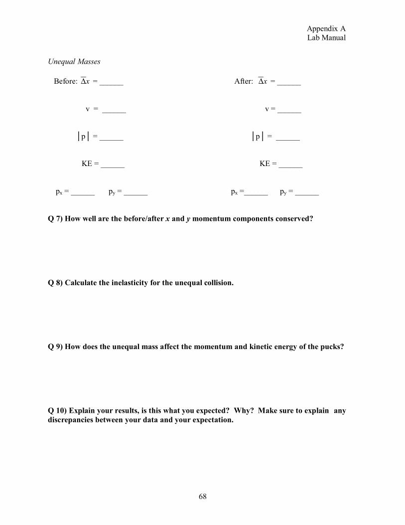
Appendix A Lab Manual
68
Unequal Masses
Before: x∆ = ______ After: x∆ = ______
v = ______ v = ______
p = ______ p = ______
KE = ______ KE = ______
px = ______ py = ______ px =______ py = ______
Q 7) How well are the before/after x and y momentum components conserved?
Q 8) Calculate the inelasticity for the unequal collision.
Q 9) How does the unequal mass affect the momentum and kinetic energy of the pucks?
Q 10) Explain your results, is this what you expected? Why? Make sure to explain any
discrepancies between your data and your expectation.
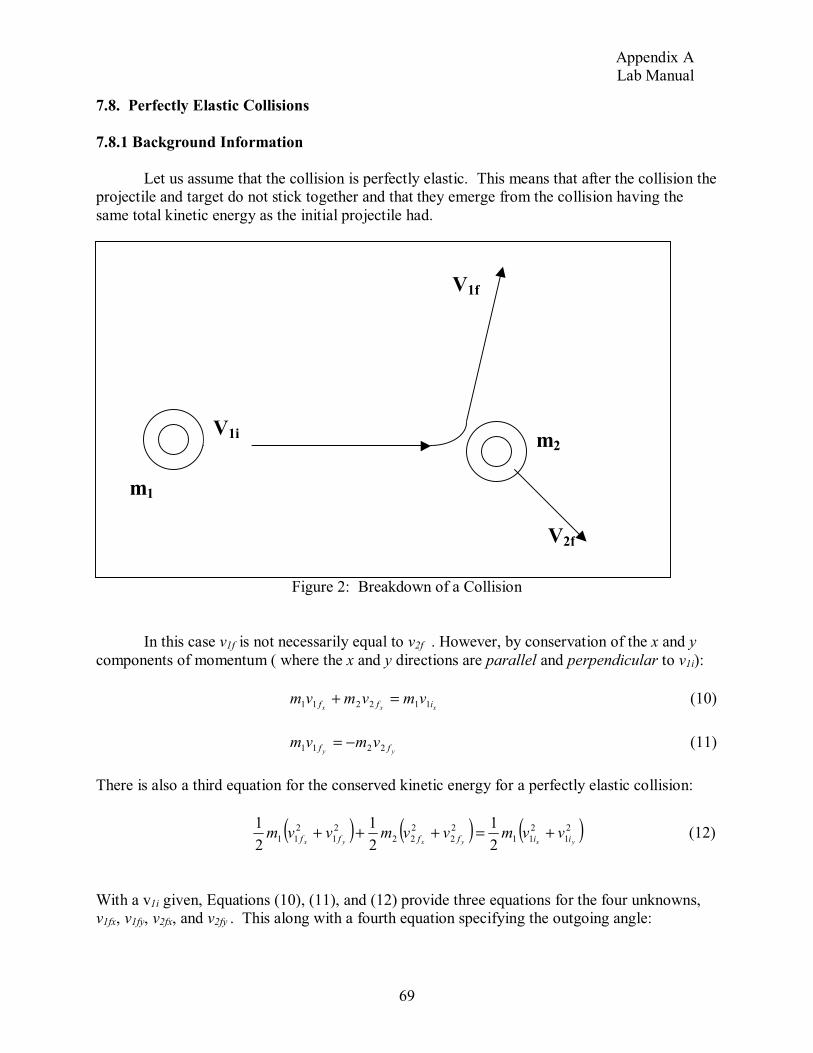
Appendix A Lab Manual
69
7.8. Perfectly Elastic Collisions
7.8.1 Background Information
Let us assume that the collision is perfectly elastic. This means that after the collision the projectile and target do not stick together and that they emerge from the collision having the
same total kinetic energy as the initial projectile had.
Figure 2: Breakdown of a Collision
In this case v1f is not necessarily equal to v2f . However, by conservation of the x and y
components of momentum ( where the x and y directions are parallel and perpendicular to v1i):
xxx iff vmvmvm 112211 =+ (10)
yy ff vmvm 2211 −= (11)
There is also a third equation for the conserved kinetic energy for a perfectly elastic collision:
( ) ( ) ( )2
1
2
11
2
2
2
22
2
1
2
112
1
2
1
2
1yxyxyx iiffff vvmvvmvvm +=+++ (12)
With a v1i given, Equations (10), (11), and (12) provide three equations for the four unknowns, v1fx, v1fy, v2fx, and v2fy . This along with a fourth equation specifying the outgoing angle:
m2V1i
m1
V1f
V2f

Appendix A Lab Manual
70
= −
x
x
f
f
fv
v
2
11
1 tanθ (13)
permits the determination of the values of the four unknowns.
7.8.2 Procedure for Elastic Collision Simulation
Equal Masses
• Place a fresh sheet of white paper on the air table and place two magnetic pucks without Velcro strips on the sheet.
• Aim the projectile puck to create a collision that, for ease of analysis, is not head-on.
• Repeat the collision procedures from part 7.8.1 under Equal Masses
Unequal Masses
• Put a lead collar on the target puck and repeat the above procedure.
7.8.3 Analysis of the Puck’s Trajectory
• Follow the procedure in part 7.6.3
7.8.4 Data Collection and Analysis
Note: for ease draw an x-axis along the initial direction the projectile puck. Use Equations (5)
and (10) through (13) to aid your analysis.
Equal Masses
Initial
Puck #1 x∆ = ______
v = ______
p = ______
KE = ______

Appendix A Lab Manual
71
px = ______ py = ______
Final
Puck #1 x∆ = ______ Puck #2 x∆ = ______
v = ______ v = ______
p = ______ p = ______
KE = ______ KE = ______
px = ______ py = ______ px =______ py = ______
Q 11) How well are the before/after x and y momentum components conserved?
Unequal Masses
Initial
Puck #1 x∆ = ______
v = ______
p = ______
KE = ______

Appendix A Lab Manual
72
px = ______ py = ______
Final
Puck #1 x∆ = ______ Puck #2 x∆ = ______
v = ______ v = ______
p = ______ p = ______
KE = ______ KE = ______
px = ______ py = ______ px =______ py = ______
Q 12) How well are the before/after x and y momentum components conserved?
Q 13) How does the unequal mass affect the momentum and kinetic energy of the
pucks?
Q 14) Explain your results, is this what you expected? Why? Make sure to explain any
discrepancies between your data and your expectation.

Appendix A Lab Manual
73
7.9 Conclusion
Analyze the similarities and differences between the explosion, the inelastic collision, and the elastic collision. Focus on the how well kinetic energy and momentum are conserved. Explain
the effects of any experimental errors.

Appendix A Lab Manual
74
8 CONSERVATION OF ENERGY—BLOCK VS. DISK ON TRACK
8.1 Purpose: To highlight the difference between translational and rotational motion while demonstrating the conservation of energy in the presence of one
or both of those.
8.2 List of Equipment
o Data Studio
o Inclined track o Calculator
o Aluminum disk mounted on small axle o Wood blocks
o Calipers o Assorted measuring tools (ruler, protractor, etc.)
8.3 Energy of Motion
In this lab, we will study energy conservation for both translational and rotational motion.
Translational motion occurs when the center of mass of the object moves, while rotational motion is when the object moves around its center of mass. A spinning top, for instance, will
have rotational motion, while a running man will have translational motion. If only translational motion is present, then the kinetic energy, as we have previously learned, will be
2
2
1MvK = (1)
where K is the total kinetic energy, M is the mass of the body, and v is the velocity of the center
of mass. As has been demonstrated, this equation is used in situations where objects move without rotation.
However, when rotation plays a factor in the movement of the object, the kinetic energy
produced by the rotation must be added to Equation 1. In that case,
22
2
1
2
1ωIMvK += (2)
Now, I is the moment of inertia for the rotating object and is the object’s angular
velocity about its center of mass. It should be noted that Equation 2 is only useful when the two terms are linked or correlated to each other—as in, the velocity and angular velocity are related
to each other by some linear equation and relationship. If there is no correlation, Equation 2 may not be used. In this lab, because the rotation of the wheel is linked to the translational velocity of
it sliding down the track, Equation 2 may be successfully utilized. Since the rotating object in this lab is a disk, it is relevant to know that, for a uniform disk with a radius of R,
2
2
1MRI = (3)
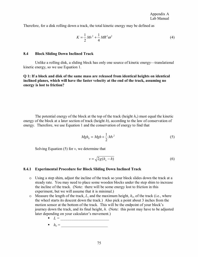
Appendix A Lab Manual
75
Therefore, for a disk rolling down a track, the total kinetic energy may be defined as
222
4
1
2
1ωMRMvK += (4)
8.4 Block Sliding Down Inclined Track
Unlike a rolling disk, a sliding block has only one source of kinetic energy—translational
kinetic energy, so we use Equation 1.
Q 1: If a block and disk of the same mass are released from identical heights on identical
inclined planes, which will have the faster velocity at the end of the track, assuming no
energy is lost to friction?
The potential energy of the block at the top of the track (height ho) must equal the kinetic
energy of the block at a later section of track (height h), according to the law of conservation of energy. Therefore, we use Equation 1 and the conservation of energy to find that
2
02
1MvMghMgh += (5)
Solving Equation (5) for v, we determine that
)(2 hhgv o −= (6)
8.4.1 Experimental Procedure for Block Sliding Down Inclined Track
o Using a step shim, adjust the incline of the track so your block slides down the track at a steady rate. You may need to place some wooden blocks under the step shim to increase
the incline of the track. (Note: there will be some energy lost to friction in this experiment, but we will assume that it is minimal.)
o Measure the length of the track, L, and the maximum height, ho, of the track (i.e., where the wheel starts its descent down the track.) Also pick a point about 3 inches from the
motion sensor at the bottom of the track. This will be the endpoint of your block’s journey down the track, and its final height, h. (Note: this point may have to be adjusted
later depending on your calculator’s movement.) L = _________________________
ho = ________________________

Appendix A Lab Manual
76
h = _________________________
o Measure the mass of the block.
M = _______________________
o Open the Data Studio Program. o Attach the motion sensor to Digital Channels 1 and 2 of the Science Workshop 750 box.
Make sure that the yellow plug is in Channel 1 and the black plug is in Channel 2. o Add the motion sensor to the Data Studio program by clicking on the “Add Sensor or
Instrument” tab in the Experiment Setup window, and selecting the motion sensor icon under the digital sensors. The motion sensor icon should appear in the experiment set up
window under the digital channels 1 and 2. o Note: You could also add the motion sensor simply by double-clicking on Digital
Channel 1 and selecting the motion sensor from that list. o Under measurements, select position and velocity only, and that the sample rate is 10 Hz.
o Under the Sampling Options tab, select the automatic stop time to be 10-15 seconds. You may need to decrease or increase this time later, depending on how fast your block
moves along your track. o In the bottom half of the Experiment Setup window, select the motion sensor tab. You
should hear a clicking sound as the motion sensor begins taking measurements. o Release the disk and press start to begin collecting data.
o Under the Display window, click the graph window and select the Position for Run 1. A graph titled “Graph 1” should appear. You can rename it by double-clicking on the
Graph 1 icon in the Display window. o Double click on the graph window. Under the Tools tab, select “Curve fit” and then hit
Ok. This should put a “Fit” button on the Graph toolbar. Under this button, select “Quadratic Fit.” Another line should appear on your graph, as well as some information
about this line of best fit. o Click the button, and select the minimum, maximum, mean, and standard deviation
values, as well as the “Show all” option. o Rearrange these boxes as needed so they do not disrupt the graph, and then print.
o Repeat with the velocity graph. o Compare the experimental value of velocity to that obtained from Equation (6).
Q 2: How accurate was the experimental value of velocity? Perform error analysis, and
discuss what accounts for any error in your result compared to the expected value?
Q 3: Did the velocity of the block increase as it slid down the track? Why or why not?
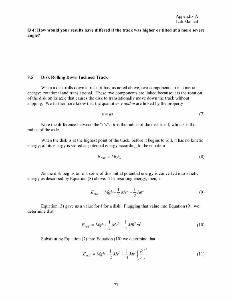
Appendix A Lab Manual
77
Q 4: How would your results have differed if the track was higher or tilted at a more severe
angle?
8.5 Disk Rolling Down Inclined Track
When a disk rolls down a track, it has, as noted above, two components to its kinetic
energy: rotational and translational. These two components are linked because it is the rotation of the disk on its axle that causes the disk to translationally move down the track without
slipping. We furthermore know that the quantities v and are linked by the property
rv ω= (7)
Note the difference between the “r’s”: R is the radius of the disk itself, while r is the radius of the axle.
When the disk is at the highest point of the track, before it begins to roll, it has no kinetic
energy; all its energy is stored as potential energy according to the equation
oTOT MghE = (8)
As the disk begins to roll, some of this initial potential energy is converted into kinetic energy as described by Equation (8) above. The resulting energy, then, is
22
2
1
2
1ωIMvMghETOT ++= (9)
Equation (3) gave us a value for I for a disk. Plugging that value into Equation (9), we determine that
222
4
1
2
1ωMRMvMghETOT ++= (10)
Substituting Equation (7) into Equation (10) we determine that
2
22
4
1
2
1++=
r
RMvMvMghETOT (11)

Appendix A Lab Manual
78
From the law of conservation of energy, we know that Equation (11) must equal Equation (8). After simplifying, we determine that
( ) +=−
2
2
4
1
2
1
r
Rvhhg o (12)
By rearranging and simplifying, we can determine the velocity of the rolling disk to be
( )
2
2
4
+
−=
r
R
hhgv o (13)
8.5.1 Disk Rolling on Track Experimental Procedure
o Using the step shim, adjust the height of the inclined track so that the disk rolls smoothly
and steadily down in a straight line. (If necessary, place a textbook or other object under the step shim to increase the initial height.) Make sure the wheel does not scrape the
sides of the track. The maximum height and length of the track should be same as the last section, but you may want to pick a different ending spot (and height) for the disk.
L = _____________________
ho = _____________________
h = ______________________
o Measure the mass of the disk.
M = _____________________
o With calipers, measure the radii of the disk (R) and of its axle (r).
R = _____________________
r = ______________________
o Under the Sampling Options tab, select the automatic stop time to be 20 seconds. Again, this time may be adjusted if needed.
o Release the disk and press start to begin collecting data. o As in the previous section, prepare and print the position vs. time and velocity vs. time
graphs using the data collected for the disk rolling down the track. o Compare the experimental value of velocity to that found in Equation (13).

Appendix A Lab Manual
79
Q 5: What, if anything, was different about the velocity of the disk compared to the
velocity of the “block?” Explain any differences.
Q 6: How accurate was the experimental velocity compared to the theoretical value?
What was the level of error, and what were possible sources of error?
Q 7: What would have happened to your results if you had used a disk with a smaller
radius? A disk with a larger axle?
Appendix B Student Survey
80
PHYSICS 101 LAB EVALUATION
Name:
Please answer all questions in regards to LAB 7: CONSERVATION OF LINEAR
MOMENTUM that you preformed in CLASS, not for extra credit
For the first 5 questions please answer using a 1-5 scale where 1=very good, 2=somewhat good, 3=neutral, 4=somewhat bad, and 5= very bad
1) How was the layout of this lab compared to other labs you have done?
2) How clear were the procedures?
3) How did the order that the information was presented in aid your understanding of the lab?
4) How clear were the informational sections compared to other labs you have done?
5) How effective were the data and analysis sections in aiding your understanding of the
material?
What were the concepts taught in this lab?
What parts of the lab did you like? Why?
What parts of the lab did you like the least? Why?
Is there any part of the lab that you feel is ineffective, confusing, or unnecessarily complicated?

Appendix C Works Cited
81
Works Cited
Carnduff, John and Reid, Norman. Enhancing undergraduate chemistry laboratories: Pre- laboratory and post-laboratory exercises. London: Royal Society of Chemistry, 2003.
Cox, Anne J. and Junkin, William F. “Enhanced student learning in the introductory physics
laboratory.” Physics Education 37, no.1 (January 2002).
Etkina, Eugenia, Murthy, Sahana, and Zou, Xueli. “Using introductory labs to engage students in experimental design.” American Journal of Physics 74 (November 2006).
Johnstone, A.H., Watt, A., and Zaman, T.U. “The students’ attitude and cognition change to a
physics laboratory.” Centre for Science Education 33, no. 1 (1998).
Laboratory Manual: General Physics 101, The College of William and Mary, 2006.
Nelson, Jane and Nelson, Jim. “Learning Cycle Model of a Science Lesson.” The Physics Teacher 44 (September 2006).